Study of sediment transport processes using Reynolds...
205
FACULTY OF ENGINEERING Department of Mechanical Engineering Study of sediment transport processes using Reynolds Averaged Navier-Stokes and Large Eddy Simulation Thesis submitted in fulfilment of the requirements for the award of the degree of Doctor in de ingenieurswetenschappen (Doctor in Engineering) by Patryk Widera August 2011 Advisor: Prof. Chris Lacor
-
Upload
truongquynh -
Category
Documents
-
view
216 -
download
0
Transcript of Study of sediment transport processes using Reynolds...

FACULTY OF ENGINEERING Department of Mechanical Engineering
Study of sediment transport
processes using Reynolds
Averaged Navier-Stokes and
Large Eddy Simulation
Thesis submitted in fulfilment of the requirements for the
award of the degree of Doctor in de ingenieurswetenschappen (Doctor in Engineering) by
Patryk Widera
August 2011
Advisor: Prof. Chris Lacor


Abstract
Sedimentation processes play a crucial role in human environment. Nu-merous examples of sediment transport and sedimentation problems canbe given, e.g. unwanted dust in our living areas, dust in electronic devices,problems with deposition efficiency of inhaled medicines, problems withuncontrolled sand transport in rivers or with transport of any kind of pol-lutants in water or in the air and industrial examples as pneumatic trans-port or cyclone separation. Contemporary knowledge about the processesthat are involved in the particle transport, in the inter-particle or fluid-particle coupling is still very small. The prediction of sediment behaviorin industrial calculations usually is based on simple, empirical formulas,which are applicable only for simple and very specific cases. Even withsuch an approach, the error of the prediction of sediment concentrationcan reach dozens or hundreds of percents. The sediment concentration er-ror can be even bigger in large areas as lakes, rivers or harbors, where theamount of variables influencing the sediment transport is larger and lesspredictable.However, the improvement of the numerical methods and computing powerraise a distinct possibility to develop more advanced models that can givethe solution to sediment transport issue in a relatively short time withreasonably high accuracy. The increasing computational power allows touse such methodologies as, e.g. Large Eddy Simulation (LES) or DirectNumerical Simulation (DNS) in order to try to investigate the patternsof sediment transport in turbulent flows. Unsteady simulations give theopportunity to investigate particle behavior on the smallest scales, whichis necessary to understand the physics of particle movement and particleresponse to turbulent fluid motions.The main goal of this thesis is to develop an efficient numerical algorithmto simulate sediment transport in the presence of turbulent flows.
The current study is based on the LES approach, where advanced sub-grid scale models are used to capture small scales of unsteady turbulentflows, i.e. the Smagorinsky and the WALE (Wall-Adapting Local Eddy)based models. In most of the considered cases the dilute flow assumptionis applied, i.e. the sediment concentration is small enough to consider itsinfluence to flow field as negligible. The only exception is the study pre-sented in Chapter 8, where the sediment phase is coupled with the fluidphase using the varying viscosity and settling velocity model. In case when

dilute flow is considered, the sediment concentration profiles are validatedagainst the theoretical curve calculated based on the Rouse equation.As first, the sediment transport in an open and closed channel with smoothwalls was studied. The results presented in Chapter 5 show good agree-ment of the LES based sediment concentration when compared to the the-oretical curve. Additionally, it is shown that the RANS solution can be im-proved when the turbulent Schmidt number is defined based on the LESsolution, when dilute flow condition is assumed.
In Chapter 6, the study of the sediment transport in the rough bottomchannel is presented. The LES solution obtained from the rough bottomsimulations were used to study the sediment transport patterns and alsoserved as reference data for development of the two-equation turbulencemodel in Reynolds Averaged Navier-Stokes framework, see Heredia [55].
The basic, classical sediment-fluid coupling models are studied and de-scribed in Chapter 8. The coupling between fluid and sediment is basedon the varying viscosity and varying settling model, i.e. model of Todaand Hisamoto [131] and Van Rijn [148], respectively. As it was expected,obtained results confirmed that even a relatively small amount of the sed-iment particles (in this case the volumetric concentration is 1 and 2%) caninfluence the flow field. It is also confirmed that the small particles influ-ence the flow field less, when compared to the influence of bigger particles,assuming the same volumetric concentration.
Chapter 9 presents the study of the slip velocity models proposed by Man-ninen et al. [84]. As has been proved, the velocity and the pressure basedmodels significantly improve solution accuracy of the Eulerian model forlarge particles, especially in the developed flow region. However, it is foundthat neglecting the turbulent and the viscous stresses results in low accu-racy in the wall vicinity. Hence, it is suggested that the near wall proper-ties of both models should be further investigated. Additionally, a simplecorrection method for the pressure based model is presented.
As has been shown in the study, the applied methodology, i.e. sedimenttransport using LES, can give a very detailed picture of the sediment be-havior, including sediment concentration, its response to the turbulentfluctuations and sediment transport patterns. Nevertheless, to recognizeresults of numerical simulations as fully correct, they should also be vali-dated against experimental results. That still seems to be an unresolvedproblem in some cases, e.g. flows with high concentration of particles.
ii

... to my grandfather Alojzy
iii

iv

Acknowledgments
First and foremost, I would like to thank to Prof. Chris Lacor for givingme possibility to do a PhD under his guidance. I would also like to grate-fully acknowledge technical supervision of Prof. Chris Lacor, especially forour weekly technical meetings and many valuable suggestions he gave meduring my PhD research.
I am greatly indebted to Prof. Erik Toorman, who helped me to discoverworld of sedimentation processes. I thank him for valuable suggestionsand interesting talks during our meetings.
I warmly thank to our system and laboratory administrator Alain Wery,for his tremendous support during my research.
I would also like to thank to our secretary, Jenny D’haes. For her supportwith translation from Dutch/French to English and filling out of plenty ofdocument forms.
It was my pleasure to work with Ghader Ghorbaniasl. I am greatly in-debted for his help in mathematical and philosophical matter. I also grate-ful for his support in moments of doubts.
It is was my pleasure to share room with very silent and patient SanthoshJayaraju. I will newer forget our talks and nice atmosphere in our room.
I am pleased to work with two new colleagues Vivek Agnihotri and FlorianKrause. They came to VUB only few months ago, however, during thisshort period we already had many valuable discussions, e.g. on particledispersion.
I am very pleased to acknowledge my present and former colleagues MahdiZakyani, Willem Deconinck, Khairy Elsayed, Kris Van den Abeele, Sergey
v

Smirnov, Matteo Parsani, Dean Vucinic, Nikolay Ivanov, Cristian Dinescu,Jan Ramboer, Tim Broeckhoven and Mark Brouns, for their support andnumerous valuable discussions.
I would also like to thank to Fonds voor Wetenschappelijk Onderzoek (FWO).My study would be impossible if not their financial support under contractG.0359.04. This support is gratefully acknowledged.
Lastly, and most importantly, I would like to thank to my parents, mygrandparents (especially to my grandfather Alojzy), my brother, and ofcourse to my wife Joanna, for their constant support and to my childrenSzymon and Anna Maria, for making me laugh even in very difficult mo-ments.
vi

Jury Members
President Prof. Hugo SolVrije Universiteit Brussel
Vice-President Prof. Rik PintelonVrije Universiteit Brussel
Secretary Prof. Gert DesmetVrije Universiteit Brussel
External Members Prof. Erik ToormanKatholieke Universiteit Leuven
Prof. Gerard DegrezUniversite Libre de Bruxelles
Internal Members Prof. Florimond De SmedtVrije Universiteit Brussel
Prof. Margaret ChenVrije Universiteit Brussel
Promoters Prof. Chris LacorVrije Universiteit Brussel
vii

viii

Contents
Nomenclature xiii
1 Introduction 11.1 The sedimentation problem . . . . . . . . . . . . . . . . . . . 11.2 Types of sediment and sediment transport . . . . . . . . . . 61.3 Types of sediment transport modeling approach . . . . . . . 81.4 Problem of scales . . . . . . . . . . . . . . . . . . . . . . . . . 101.5 Outline of the work . . . . . . . . . . . . . . . . . . . . . . . . 13
2 Governing Equations 172.1 Conservation Equations for Fluid and Sediment . . . . . . . 172.2 Pressure correction method . . . . . . . . . . . . . . . . . . . 202.3 Time discretisation method . . . . . . . . . . . . . . . . . . . 21
3 Turbulence modeling 233.1 Nature of turbulence . . . . . . . . . . . . . . . . . . . . . . . 233.2 Turbulence modeling . . . . . . . . . . . . . . . . . . . . . . . 263.3 RANS model . . . . . . . . . . . . . . . . . . . . . . . . . . . . 273.4 LES models . . . . . . . . . . . . . . . . . . . . . . . . . . . . 28
3.4.1 Constant Smagorinsky model . . . . . . . . . . . . . . 293.4.2 Constant Wale model . . . . . . . . . . . . . . . . . . . 303.4.3 Dynamic Smagorinsky model . . . . . . . . . . . . . . 313.4.4 Dynamic Wale model . . . . . . . . . . . . . . . . . . . 333.4.5 Dynamic Smagorinsky for the sediment equation. . . 373.4.6 Dynamic Wale for the sediment equation . . . . . . . 38
4 Particle settling velocity 414.1 Non-cohesive sediment . . . . . . . . . . . . . . . . . . . . . . 414.2 Drag in still fluid . . . . . . . . . . . . . . . . . . . . . . . . . 424.3 Cohesive sediment . . . . . . . . . . . . . . . . . . . . . . . . 484.4 Influence of turbulence to the particle settling velocity . . . 51
ix

4.5 Settling velocity in sedimented fluid . . . . . . . . . . . . . . 534.6 Summary . . . . . . . . . . . . . . . . . . . . . . . . . . . . . . 55
5 Application 1 - Sediment transport in an open channel flow 575.1 Introduction . . . . . . . . . . . . . . . . . . . . . . . . . . . . 585.2 Description of the test cases . . . . . . . . . . . . . . . . . . . 595.3 Carrier flow results . . . . . . . . . . . . . . . . . . . . . . . . 615.4 Sediment transport results . . . . . . . . . . . . . . . . . . . . 615.5 Test case summary . . . . . . . . . . . . . . . . . . . . . . . . 80
6 Application 2 - Sediment transport over rough bottom 816.1 Introduction . . . . . . . . . . . . . . . . . . . . . . . . . . . . 826.2 Description of the test cases . . . . . . . . . . . . . . . . . . . 836.3 Carrier flow results . . . . . . . . . . . . . . . . . . . . . . . . 856.4 Sediment transport results . . . . . . . . . . . . . . . . . . . . 876.5 Test case summary . . . . . . . . . . . . . . . . . . . . . . . . 101
7 Coupling between sediment and fluid 1037.1 Introduction . . . . . . . . . . . . . . . . . . . . . . . . . . . . 1037.2 Viscosity coupling methods . . . . . . . . . . . . . . . . . . . . 1057.3 Density coupling . . . . . . . . . . . . . . . . . . . . . . . . . . 1077.4 Momentum coupling . . . . . . . . . . . . . . . . . . . . . . . 1087.5 Summary . . . . . . . . . . . . . . . . . . . . . . . . . . . . . . 114
8 Application 3 - Investigation on sediment and fluid coupling,standard methodologies 1178.1 Introduction . . . . . . . . . . . . . . . . . . . . . . . . . . . . 1188.2 Description of the test cases . . . . . . . . . . . . . . . . . . . 1198.3 Carrier flow results . . . . . . . . . . . . . . . . . . . . . . . . 1208.4 Sediment transport results . . . . . . . . . . . . . . . . . . . . 1268.5 Test case summary . . . . . . . . . . . . . . . . . . . . . . . . 135
9 Application 4 - Investigation on sediment and fluid coupling,the drift flux model 1379.1 Introduction . . . . . . . . . . . . . . . . . . . . . . . . . . . . 1389.2 Description of the test cases . . . . . . . . . . . . . . . . . . . 1399.3 Carrier flow results . . . . . . . . . . . . . . . . . . . . . . . . 1409.4 Test case summary . . . . . . . . . . . . . . . . . . . . . . . . 151
10 Conclusions and Perspectives 15310.1 Conclusions . . . . . . . . . . . . . . . . . . . . . . . . . . . . 15310.2 Perspectives . . . . . . . . . . . . . . . . . . . . . . . . . . . . 156
APPENDIX 159
x

List of Publications 167
Bibliography 170
Outline 187
xi

xii

Nomenclature
B Logarithmic law coefficientC Sediment mass concentration [kg/m3]Cs Smagorinsky model coefficientCw WALE model coefficientCD Drag coefficientCL Lift coefficientCε1,Cε2 k − ε model coefficientCµ Eddy viscosity model coefficientdk sgs sediment fluxDk sgs sediment fluxDMpij Diffusion term in continuity equation for a dispersed phase
D Sediment diffusivity coefficient [m2/s]Dt Turbulent diffusivity coefficient based on RANSDsgs, D
sgsTurbulent diffusivity coefficient based on sgsDres Turbulent diffusivity coefficient based on resolved scalesDLES Turbulent diffusivity coefficient based on resolved and sgs
scales: DLES = Dres +Dsgs
DV D Van Driest damping functionE Source term in k − ε modelFD Drag force [N ]FG Gravity force [N ]FB Buoyancy force [N ]G∆(x) Filtering function in LESLij Leonard stress tensor in sgs modelMp Drag induced momentum transferMij Tensor in sgs modelN Cell numberPk Turbulence kinetic energy production term in RANSReτ Reynolds number based on the mean wall friction velocityReb Reynolds number based on the bulk velocity
xiii

Rep Particle Reynolds number based on the particle diameterand the particle slip velocity
Ret Turbulent Reynolds numberSij Strain rate tensor|S| Tensor multiplication, depends on the sgs modelSt Stokes numberTij Subtest scale stress tensorTi Turbulence intensityTt Turbulent time scaleVp Particle volume [m3]Vs Sediment volume [m3]Vtot Total volume occupied by sediment and fluid phase [m3]V Cell volume [m3]Z Rouse parameter
a Wave amplitude [m]af,max Fluid acceleration [m/s2]dp Particle diameter [m]gi Gravitational acceleration in i− th direction [m/s2]fi Body force [N ]fµ Damping function in k − ε modelf2 Damping function in k − ε modelh Height, e.g. channel height [m]k Kinetic energy of turbulence [m2/s2]k+ Nondimensional roughness heightl Length scale of the energy containing eddiesq Volumetric fraction of sediment concentration q = Vs/Vtotqs Sediment concentration according to Rouse equationqa Sediment concentration at the reference height yaqp Phase p in mixture approach, e.g. sediment concentrationqk Phase k in mixture approachqs Initial Sediment concentrationqm Maximum sediment volumetric concentrationp Pressure [Pa]pm Pressure of the mixture [Pa]pp Pressure of the phase p [Pa]t Time [s]
u′
Fluctuation of the flow velocity [m/s]
u′
l Large scale velocity fluctuation [m/s]√<u′u′>u∗
Nondimensional RMS value of the velocity fluctuation< u
′v′> Reynolds shear stress [m2/s2]
xiv

u∗ Wall friction velocity [m/s]u∗fit Wall friction velocity based on best fit approximation [m/s]u∗i Velocity component at the intermediate step [m/s]umi Cartesian component of the mixture velocity [m/s]upi Cartesian component of the velocity of phase p [m/s]ui Cartesian component of the velocity vector [m/s]
uslipi Cartesian component of the slip velocity vector [m/s]umki Cartesian component of the phase diffusion velocity [m/s]urms RMS of the fluid velocityu Streamwise velocity component [m/s]v Wall normal velocity component [m/s]w Spanwise velocity component [m/s]xi Cartesian component of the coordinate vector [m]u∗ Wall friction velocity [m/s]vs Settling velocity [m/s]vscf Settling velocity in a clear fluid [m/s]vsavg Average settling velocity [m/s]y+ Nondimensional heightya Reference height used in Rouse equationx, y, z Cartesian coordinates [m]β Inverse of the turbulent Schmidt number4x+ Nondimensionalized cell size in x direction4y+ Nondimensionalized cell size in y direction4z+ Nondimensionalized cell size in z directionδij Kronecker deltaε Turbulent kinetic energy dissipation [m2/s3]λw Wave length [m]µ Dynamic fluid viscosity [kg/(m ∗ s)]µm Mixture viscosity [kg/(m ∗ s)]ν Kinematic viscosity (ν = µ/ρ) [m2/s]νt Eddy viscosity [m2/s]ρ Density [kg/m3]ρf Clear fluid density [kg/m3]ρp Particle density [kg/m3]ρm Mixture density [kg/m3]κ Von Karman coefficient κ = 0.41σij Viscous stress tensorσt Turbulent Schmidt numberσres Turbulent Schmidt number based on resolved scalesσsgs Turbulent Schmidt number based on sgs scalesσk Turbulent Schmidt number for kinetic energyσε Turbulent Schmidt number for dissipation rate
xv
τsgsij Subgrid scale stress tensorτGmij Sum of viscous and turbulent stressesτw Wall shear stress [N/m2]τp Particle relaxation time [s]τK Kolmogorov time scale [s]τe Turnover time of large eddy [s]Ωij Rotation rate tensor
Subscripts
b Bulk velocityl Large scaleres Resolved quantitysgs Subgrid-scale quantityt Turbulent quantity∞ Free stream or ambient conditions
Superscripts
sgs Subgrid scale∼ Favre filtered quantity− Spatially filtered quantity′′ Unresolved quantity′ Resolved fluctuation+ Nondiemsionlized quantity〈. . . 〉 Time and/or space averaged quantity
Abbreviations
CFD Computational Fluid DynamicsCFL Courant-Friedrichs-Lewy numberDNS Direct Numerical SimulationLES Large Eddy SimulationRANS Reynolds Averaged Navier-StokesDNS Direct Numerical SimulationCV Control VolumeFV Finite VolumeR-K Runge-KuttaWALE Wall-Adapting Local Eddy-viscosityFTBV Fast Tracking Between Vortices
xvi

Chapter 1
Introduction
Contents1.1 The sedimentation problem . . . . . . . . . . . . . . . . 11.2 Types of sediment and sediment transport . . . . . . 61.3 Types of sediment transport modeling approach . . 81.4 Problem of scales . . . . . . . . . . . . . . . . . . . . . . 101.5 Outline of the work . . . . . . . . . . . . . . . . . . . . . 13
1.1 The sedimentation problemThe natural transport of sediments is one of the most common and themost important processes in human environment. Sedimentation occursalmost everywhere in nature: in rivers, lakes, seas or even in the air inthe form of dust, smoke which leaves black carbon spots on walls or smogbeing a mixture of pollution and fog, as well as all kinds of chemical pollu-tants etc. Sedimentation may pertain to objects of various sizes, rangingfrom huge rocks to suspensions of pollen particles. Suspended particletransport can be extensively used in industrial applications, e.g. pneu-matic transport of powder materials.One of the brightest and, unfortunately, extremely expensive examples ofsedimentation processes has been experienced in Australia, which givesan idea how important is it to get knowledge about sediment transport,its settling and erosion. Several dams that have been build to supplyfresh water to cities and villages, predicted to serve for at least fifty years,had to be closed after less than 50% of their expected lifetime, see fig-ure 1.1, where results of unpredicted sedimentation in Cunningham andKoorawatha Creek dam (both in Australia) are presented.
1

CHAPTER 1. INTRODUCTION
Figure 1.1: Left: Cunningham Creek dam (1912) : railway dam fully-silted in lessthan 20 years (HardenNSW,Australia). Right: Fully silted Koorawatha Creekdam (1911). (www.iahr.org)
Table 1.1: Major reservoir siltation in Australia, see Chanson [23], (www.iahr.org).
Reservoir Location Start of use End of useSheba dams Nundle NSW 1888 – (*)Corona Broken Hill NSW 1890 1910(*)Laanecoorie Maryborough VIC 1891 SIUStephens Creek Broken Hill NSW 1892 SIUJunction Reefs Lyndhurst NSW 1896 1930(*)Moore Creek Teamworth NSW 1898 1924(*)Gap Werris Creek 1902 1924(*)Koorawatha Cowra NSW 1911 – (*)Pykes Creek Ballan VIC 1911 SIUPekina Creek Orroroo VIC 1910 1930(*)Cunningham Creek Harden NSW 1912 1929(*)Illalong Creek Binalong NSW 1914 1985(*)Umberumberka Broken Hill NSW 1915 SIUMelton Werribee VIC 1916 SIUKorrumbyn Creek Murwillumbah NSW 1918 1924(*)Quipolly Werris Creek NSW 1932 1955(*)Inverell Inverell NSW 1939 1982(*)Note: (*):reservoir fully sedimented today; (–): information not available,(NSW): New South Wales, (VIC): Victoria, (SA): South Australia,(SIU): still in use
2

CHAPTER 1. INTRODUCTION
In Table 1.1 dams built in Australia between 1890 and 1960 are presented.As it is possible to notice almost all of them after short time got fully silted.In extreme cases, some dams, have been fully silted in less than sevenyears, see Table 1.1 - Korrumbyn Creek dam. Most of dams presented inTable.1.1 were silted much earlier then their expected lifetime. However,presented dams are mentioned only to give an extreme example to whatsedimentation can lead. In reality, the processes of sedimentation or sil-tation of water reservoirs are valid all over the world, especially in aridregions∗. Hence, it is very important to understand multiple processesthat governs the sediment transport.Sediment transport is also very important in case of other water struc-tures, like rivers or channels. Water flowing in rivers is able to transportlarge amounts of suspended particles. As can be seen in figure 1.2, in someregions particles transported by water can settle and create shallow waterregions and dunes.
Figure 1.2: Left: Wisla estuary, Poland (www.maps.google.com), settled sed-iment has blocked river accessibility for ships from the streamwise direc-tion. Right: Sediment transported towards ocean, Betsiboka river, Madagascar(www.solarviews.com)
It is very important to keep sea and river shipways deep enough to ensureproper safety level for marine vessels. To avoid danger, river or estuarybottom in areas of ship pathways has to be constantly under control, and,when the water depth is becoming too low, very expensive dredging† works∗A region is said to be arid when it is characterized by a severe lack of available water, to
the extent of hindering or even preventing the growth and development of plant and animallife.(www.wikipedia.com)†Dredging is an excavation activity or operation usually carried out at least partly un-
derwater, in shallow seas or fresh water areas with the purpose of gathering up bottom sedi-ments and disposing them at a different location. This technique is often used to keep water-
3

CHAPTER 1. INTRODUCTION
have to be performed, see figure 1.3 and 1.4, where examples of dredgingmachines are shown.
Figure 1.3: (Left), (Right): dredging machines during work (www.uq.edu.au).
Figure 1.4: Examples of dredging machines. (Left) Trailing suction hopper dredg-ing vessel with own sediment hoppers (this vessel is able to transport dredgedsediment to another place autonomically), (www.dcsc.tudelft.nl) and (Right) Cut-ter dredger which transports the sediment to the disposal area by floating pipingsystem, (www.musing.nl).
It can be seen that there are different types of dredging vessels. One of thesimplest dredging units is represented in figure 1.3, where the river bottomis dredged by the excavator standing on a barge. The disadvantage of thesedredging vessels is their low speed of dredging. More advanced dredgersare presented in figure 1.4, which can be divided into two main types. The
ways navigable. It is also used as a way to replenish sand on some public beaches, where toomuch sand has been lost because of coastal erosion.
4

CHAPTER 1. INTRODUCTION
Figure 1.5: Cutter dredging head attached to the suction tube mounted on thedredging vessel (www.cadac.com).
first one, figure 1.4(left), presents an autonomic dredger of TSHD type(Trailing Suction Hopper Dredger), which removes mud and/or sand frombottom by imposing strong underpressure at the end of the dredging arm.This vessel can also transport the dredged material to disposal area. Theother type of dredging vessels, presented in figure 1.4(right), uses similardredging method ∗, however, in this case the dredged material is immedi-ately transported to disposal area by the floating piping system. There arealso other types of dredging machines, e.g. dredger which are based on thebucket transport, water jet, and many others, for more information pleaserefer to the Internet encyclopedias or professional literature.
In any case, the dredging process is slow, especially when it is compared tothe scale of applications. As an example, Table 1.2 presents the amounts oftonnes of sediment dredged in Belgium in the year 2007 and 2008. Num-bers presented in Table 1.2 can give some rough picture of the scale ofthe sedimentation problem in harbor and river applications. Moreover, thedredging process is also very expensive. For example, only in the UnitedStates, in year 2008, the costs of dredging reached about 650† million dol-lars. Hence, it is of highest importance to find methods and/or to developsome numerical tools to be able to predict the sediment behavior.
∗Additionally to underpressure, there is also cutter head mounted at the end of the dredg-ing arm. Rotating cutter head at the suction inlet is mounted to loosen the bottom layer.†Data found at US Army Corps web page (www.iwr.usace.army.mil)
5

CHAPTER 1. INTRODUCTION
Table 1.2: Example of amount of dredged material dumped at sea per calendar year(tonnes of dry substance). This table presents only the amount of dredged materialwhich is necessary to keep the proper nautical depth [76].
year quantity [tonnes of dry substance]2007 8,518,4272008 10,305,232
1.2 Types of sediment and sediment transportSediment particles can mainly be described by their size, shape and den-sity. Sediment particles are classified according to their sizes, see figure1.6.However, in reality, sediments (either suspended or on the channel bed)are never of the same size. The spectrum of their size can vary from mi-crometers up to centimeters, at the same time, in the same flow. This isone of the most challenging problems of the sedimentation investigations.Basically, sediment can be divided into two main families, dependently ontheir way of interaction with carrier and in between sediment particles,i.e. there are cohesive and non-cohesive sediments.The cohesive sediment usually is a mixture of very fine particles, e.g.clay, silt and organic material. Cohesive particles are attracting each otherdue to the electrochemical processes, and as result they are tending tomerge into bigger objects, referred to as ”flocs”. Flocs behave differentlythan small particles. Flocs influence the flow patterns in a different waythan a group of separate particles with the same volume. Flocs can alsobreak into smaller flocs due to floc-flow interaction. The strength and thesize of the flocs depends on the material properties of the smallest particlesand the flow properties. Due to very complicated pattern of the floc cre-ation, and its breaking, the cohesive sediment transport research is verycomplicated and up till now investigated only to a limited extent.The non-cohesive sediments are defined as particles where the elec-trochemical interaction between particles is negligible, and due to theirown mass, inertia and material they are made of, these particles are notforming into flocs (in suspension). In the present dissertation only the noncohesive sediment transport will be investigated and described. A smallsubsection on cohesive sediment can be found in the chapter about cou-pling methods.Transport of the sediment it is a very complicated process. However, it canroughly be divided into two main types:Suspended in fluid - particles are light enough to be kept flowing in thewater and carried away by the stream. This situation takes place when
6

CHAPTER 1. INTRODUCTION
Figure 1.6: Correlation chart showing the relationships between phi sizes, millime-ter diameters, size classifications, ASTM and Tyler sieve sizes. Chart also showsthe corresponding intermediate diameters, grains per milligram, settling veloci-ties, and threshold velocities for traction (www.woodshole.er.usgs.gov).
7

CHAPTER 1. INTRODUCTION
Figure 1.7: Patterns of particle transport.
the gravitational flux is in balance with the turbulent flux.Bed load - in this transport mode, particles are too heavy to be in sus-pension, however they are light enough to be moved by the forces exertedby the acting fluid. Movement of particles in this mode usually is due torolling, sliding and saltation.The amount of the sediment load that can be transported by the carrierdepends on many factors, e.g. fluid velocity, carrier turbulence level, shapeand roughness of the bottom, type of the sediment in the water and itsinteraction with water and in between particles.
1.3 Types of sediment transport modeling ap-proach
The existing methods of dealing with the particulate phase can be dividedinto two main frameworks, the Lagrangian and the Eulerian approach.In the Lagrangian method, particles are defined as points or small spheresthat are traveling with the flow. For each separate particle, one equation ofmotion has to be solved. As a consequence, even in dilute suspensions theamount of particles that have to be tracked is large, which requires moreCPU power or increased computational time. Additionally, as the size ofthe particles is decreasing, and the volume of the particle has to be kept atthe same level, the amount of particles that have to be tracked is dramati-cally rising, implying that the computational time is becoming enormouslylarge to get a statistically steady solution. Thus, this technique is a veryimportant and useful tool mainly for very small scale application (e.g. par-ticle tracking in lungs) and for the scientists. Unfortunately, it is compu-tationally too expensive to be useful in large scale flows or in engineering
8

CHAPTER 1. INTRODUCTION
applications, where the solution has to be obtained in a reasonably shorttime, i.e. in a few hours or a few days, at most.
The Eulerian methodology deals with particles in the same manner as withthe fluid phase. The particulate phase is described as a continuum wherethe transport equations are very similar to these which describe the car-rier fluid phase. The Eulerian modeling technique can be used not onlyfor modeling of the sand particles, but it can also be used for modelingof transport and dispersion of secondary fluids, e.g. oil spills in water,which is impossible in the case of a Lagrangian framework. The Eulerianmethodology is also much more efficient than the Lagrangian one, fromcomputational time efficiency point of view. However, it is more difficultto describe properly the boundary conditions or to estimate e.g. the slipvelocities or influence of the particles on the fluid viscosity or turbulencelevel in the flow.
It can be stated that each of the aforementioned methods has its advan-tages and disadvantages. This also means that each of these methods issuitable for different fields of applications. The Lagrangian methodologyis more suited for very diluted flows, with particles with relatively big in-ertia (large or/and heavy particles), whereas the Eulerian methodology ismore suited for flows with very fine particles, with low inertia and also formulti-fluid modeling.
In reality, except for some laboratory cases, sediment particles in naturalenvironment are never of the same size. Usually, there is a mixture of dif-ferent size particles, from clay size (order of dozens of micrometers) andsmall sand up till gravel (order of centimeters). This makes any modelingprocess complicated. For time being it seems to be not possible to createa very complex code with the treatment of both lagrangian particles andEulerian phase ∗. It has been assumed that the developed code should betreated with sediment which is the most common in rivers, i.e. with smalland very small sand particles. These particles can already be modeledwith the Eulerian framework. Because of that, in this thesis, the Eulerianmethodology has been chosen. This method is more efficient than the La-grangian one for sediment transport in rivers, being also easier to apply toengineering modeling.
∗Theoretically it is possible, however, it would be very time consuming for any practicaluse.
9

CHAPTER 1. INTRODUCTION
1.4 Problem of scalesIt is of highest importance to upgrade existing numerical models and/or todevelop more sophisticated tools for the prediction of sediment transportpattern and its influence on the environment. The major problem of cre-ating numerical tools for sediment transport applications arises from thefact that the range of sizes of the fluid and particle phase, which have tobe resolved, is very wide. The sediment particles usually are consideredas very small, i.e. it can be assumed that their size is varying in rangefrom micrometers up to centimeters. Also, it is well known that, in a tur-bulent flow, there is the whole range of turbulent scales varying from theKolmogorov scales up to large scale flow structures which, in the currentapplications, can easily reach sizes of up to hundreds of meters∗. Com-paring particle and fluid scales that have to be resolved with the scalesof computational domains, i.e. with e.g. river estuaries, it becomes clearthat it is not possible to create meshes fine enough to cover all scales andresolve them directly. For simulations of e.g. a river estuary the computa-tional domain has to cover large areas, very often it is a matter of manysquare kilometers, see examples of computational domain of Scheldt andChangjiang river estuary given in Table 1.3 and visualized in figure 1.8.
Table 1.3: Example of grid cell size in models used in simulation of flow and sedi-ment transport in river estuaries.
model of cell size [m] vert. resolutionScheldt estuary [34] 150 m - 30000 m 1 (2D)Scheldt estuary [145] 50 m - 400 m 5Changjiang estuary [83] 100 m - 2000 m 20
As it is easy to notice (Table 1.3), the average resolution of the meshesused in the above examples is of the order of dozens of meters. This simplymeans that all scales which are smaller than the mesh cells cannot beresolved, but have to be modeled. The suitability of different numericalapproaches for the use in some typical applications, are roughly indicatedin figure 1.9.Hence, it is important to create proper numerical models to calculate thesubgrid-scale behavior of fluid motions and particle transport patterns.However, to validate the developed models, reference data are needed.Data used for validation can be based on laboratory measurements or ob-
∗In reality, large flow scales can reach dimensions of thousands of kilometers, e.g. oceancurrents. However, these flow scales are usually neglected in estuarial sediment transportmodeling.
10

CHAPTER 1. INTRODUCTION
Figure 1.8: Example of NeVla (Nederlands en Vlaams) grid for flow and sedimenttransport modeling in Scheldt estuary [88]. (Left), complete computational do-main, (right) part of the computational domain. Visible simplifications of the rivershape, i.e. the complex shape of the river bank is not well represented by the meshcells. Note also, that the computational grid is wider than the river itself to includethe planned widening of the river.
tained from numerical simulations which have been validated and theiraccuracy has already been proved.There are several models in CFD (Computational Fluid Dynamics) thatcould possibly be used for studying sedimentation transport processes. Thebest known are DNS (Direct Numerical Simulation), LES (Large EddySimulation) and RANS (Reynolds Averaged Navier Stokes). The most ac-curate models would result from a DNS approach. In this case, all flowscales are computed directly. The main drawback of this methodology isthe need for very fine meshes ∗, which results in very high computationaltimes. Thus, the range of application is limited mainly to cases where therange of scales is limited, i.e. typically low Reynolds number flows†, seefigure 1.9. On the other hand, the RANS approach is much faster. Never-theless, its accuracy and the amount of information it provides about theturbulent flow is limited, mainly because all turbulent flow scales have tobe modeled. Taking into account the required solution accuracy, and thesimulation time, the LES approach seems to be the most relevant model forstudying sediment transport processes in small scale flows. Hence, for thisstudy, LES has been used to perform small scale simulations of the sedi-
∗The mesh has to be fine enough to cover all flow scales, up to the Kolmogorov scale†It is possible to use LES and DNS for large scale flows. However, for such large scale
applications machines with thousands of processors have to be used to fulfill the cpu powerdemand which is needed to perform simulation in reasonable short time, e.g. in few months.
11

CHAPTER 1. INTRODUCTION
Figure 1.9: Visualization of characteristic space and time scales in oceans (vonStorch et al., 1999). With red, blue and green rectangles regions of usability iffollowing numerical methods are presented, i.e. red color corresponds to DNS, bluecorresponds to LES and green represents the RANS methodology.
ment transport. The ultimate aim of LES is to generate data to validatethe subgrid-scale models for high concentration effects near the bottom inRANS models, since most of the current measurement techniques are notyet suitable to measure the sediment concentration and the flow field inhigh concentrated suspensions.There are two main approaches for solving the fluid conservation equationsin Computational Fluid Dynamics (CFD). One is based on an incompress-ible, and the other is based on a compressible set of equations. In case ofan incompressible framework, only the fluid conservation equations needto be solved, i.e. the mass and the momentum conservation equations. Inthe incompressible approach there is no relation between the fluid densityand its pressure. While in compressible case, the fluid conservation equa-tions are combined with the energy conservation equation through someconstitutive equations, i.e. the ideal gas law. In the compressible approachthe density is allowed to vary accordingly to the pressure variations. The
12

CHAPTER 1. INTRODUCTION
compressible approach usually has to be used for flows where shock wavesoccur. However, in some cases, variation of the fluid density might also benecessary in the incompressible approach, e.g. in the sediment transport,as an effect of the particle concentration. Theoretically, using the varyingdensity framework should allow to observe some of the real-life effects, ase.g. the density currents. Hence, the set of the conservation equationsused in this study is based on the incompressible, but the varying densityapproach.To apply for the density changes when the sediment transport is consid-ered, the fluid density has to be considered as the mixture density, thatdepends on the sediment concentration. However, performed tests showedthat the mentioned approach is highly unstable when combined with cur-rently used pressure solver, i.e. the Poisson solver. Thus, for the clarity,all equations are written in terms of the varying density approach, but themixture density used during simulations is constant and equal to the fluiddensity. However, in future studies of the sediment transport the densityvariation should also be considered, as it can be of high importance, espe-cially in the bottom region and for high concentration cases.
1.5 Outline of the workThe main goal of this work is to develop an efficient numerical algorithmto compute sediment transport. This tool will allow to study the smallscale processes that occur during transport of sediment particles and toestimate which of these processes are essential and should be taken underconsideration during the development of numerical solvers for large scaleapplications. In this study the sediment is considered as a continuum, i.e.an Eulerian approach is applied. In total, there are four main cases con-sidered. First, the sediment transport equation was implemented in anexisting LES fluid solver. This allowed to perform the sediment transportstudy where the sediment phase has been considered as a passive scalar,i.e. one-way∗ coupling is assumed. In this case, a channel with one, andtwo smooth walls has been considered, i.e. an open and closed channel, re-spectively. At the next stage, the sediment transport over rough walls hasbeen investigated. In the present study, to account for the roughness ef-fects, the bottom wall has a wavy shape, with specific wave length and withthree wave amplitudes†. The third part of the sedimentation study is aboutthe classical methodologies of sediment and fluid coupling. In this case, theviscous and settling velocity coupling effects have been investigated. The
∗One-way coupling means, that only the flow field is influencing the sediment phase.†The flat bottom case has been used as a reference
13

CHAPTER 1. INTRODUCTION
fourth part of the study is about a novel way of the fluid-sediment cou-pling, which is based on an approach developed by Manninen et al.[84].They have proposed a way to calculate the sediment slip velocity∗ in anEulerian framework. This is of highest importance for sediment transportstudy of larger particles.The outline of this dissertation is as follow:Chapter 1 gives an introduction to sedimentation, where some basic defi-nitions are introduced, i.e. types of sediments are given, the transportingpatterns of sediment particles are mentioned. In this chapter also prob-lems with sedimentation processes are described. Additionally, the mainmethodologies of numerical treatment of sedimentation problems are pre-sented, and their main weaknesses and strengths are highlighted.
In Chapter 2, details of the numerical methods used are described. Inthis chapter the mass and momentum conservation equations are given,as well as the sediment transport equation. Additionally, the pressure cor-rection methodology and restrictions of the CFL number are presented.
In Chapter 3, details about the models that deal with the turbulent ef-fects are given, both for the Reynolds Averaged Navier Stokes (RANS) andLarge Eddy Simulation (LES) approach. For the RANS methodology thek− ε model is described, and for the LES framework the Smagorinsky andWALE models are proposed. The LES models can be based either on aconstant coefficient approach or on the dynamic procedure.
In Chapter 4, the parameters that are characteristic for suspended par-ticles are described.
Chapter 5, presents a detailed description of the open and closed channelflow test case with sediment transport. The comparison between RANSand LES is presented. A simple method of improving the accuracy of thesediment transport in the RANS framework is proposed. The method isbased on using a varying Schmidt number wall normal profile in a RANSbased simulations. The turbulent Schmidt profile is based on the LES so-lution. An improved accuracy as compared to standard RANS is obtained.
Chapter 6 presents results of the sediment transport in case of rough bot-toms. The results show a strong influence of the wavy bottom surface tothe pattern of sediment transport. However, it is also shown that the in-fluence of the bottom roughness to the sediment transport is decreasing
∗The slip velocity (also referred to as the relative velocity) is defined as the velocity of asecondary phase relative to the velocity of the primary phase [40].
14

CHAPTER 1. INTRODUCTION
rapidly with increasing distance to wall.
In chapter 7, the most common methods of fluid-sediment coupling that aredescribed in the literature are presented. There is also a detailed deriva-tion of the drift flux model, including all assumptions and simplifications.
In chapter 8, results of sediment-fluid coupling method based on varyingsettling velocity and viscosity are presented. The obtained results showthat even a small amount of sediment can drastically influence the flowfield, i.e. the velocity field and the turbulence level. The results also showthat the same amount of sediment will influence the flow differently if theconsidered particle sizes are different.
Chapter 9 describes results obtained with the drift flux model. The so-lution of the Eulerian based particle Reynolds number is compared to dataobtained from Direct Numerical Simulation, where particle slip velocitieswere calculated based on the Lagrangian approach. The presented resultsprove the usefulness of the drift flux model and compare fairly accurate tothe DNS solution. However, some weaknesses of the drift flux models arealso indicated.
Finally, in Chapter 10, concluding remarks are drawn and an outlook tofuture work is given.
15

CHAPTER 1. INTRODUCTION
16

Chapter 2
Governing Equations
Contents2.1 Conservation Equations for Fluid and Sediment . . 172.2 Pressure correction method . . . . . . . . . . . . . . . 202.3 Time discretisation method . . . . . . . . . . . . . . . . 21
2.1 Conservation Equations for Fluid and Sed-iment
The processes of the sediment transport in fluids such as air or water canbe described by a set of conservation equations applied to the flow and thesediment phase [57].The conservation equation of continuity and momentum in the Large EddySimulation (LES) framework for varying density flows are obtained by fil-tering the varying density Navier-Stokes equations and can be formulatedas
∂ρ
∂t+∂ρui∂xi
= 0 (2.1)
∂ρui∂t
+∂ρuiuj∂xj
= − ∂p
∂xi+
∂
∂xj[µ
(∂ui∂xj
+∂uj∂xi
)− τsgsij ] + fiδi1 (2.2)
where ui, uj are the filtered velocity components with i, j = 1, 2, 3, p is thepressure term, µ = νρ is the fluid dynamic viscosity where ν = 1.304 ∗10−6m2/s is the fluid kinematic viscosity coefficient and ρ is the suspen-sion density. The density of the clear fluid (i.e. water without particles) is
17

CHAPTER 2. GOVERNING EQUATIONS
equal to 999.8kg/m3. The water properties are taken from physical tablesassuming standard pressure and temperature of 100C. The way to obtainthe suspension density is presented at end of the section. The last term inequation 2.2, i.e. fi, is a body force (source term) that ensures sustainingthe proper velocity of the fluid when a channel with periodic streamwiseboundary conditions is considered. The body force is based on the smoothbottom friction velocity u∗ and calculated using the following expression
fi =u2∗ρ
h(2.3)
where h is the channel height. τsgsij in equation (2.2) is the subgrid scalestress defined as
τsgsij = ρ(uiuj − uiuj) (2.4)
Note that, although the code is incompressible, the density which is themixture density can vary according to the sediment concentration, seeequation 2.11. The varying density requires the use of a Favre [41] filter-ing operator to uncouple the velocity field from the varying density field,see e.g. Piomelli [109]. The Favre [41] filtered value of any quantity ψ isdenoted as ψ and defined as:
ψ =ρψ
ρ(2.5)
where the ’-’ symbol represents the filter operator. The conservation equa-tion for the sediment is given by
∂ρsq
∂t+∂ρs[(uj − vsδj3)q]
∂xj= − ∂
∂xj
[(D +Dsgs)
∂q
∂xj
](2.6)
where q is the Favre [41] filtered volumetric sediment concentration, ρs =2650kg/m3 is the sediment density, δj3 is the Kronecker delta which en-sures that the settling velocity will work only in one direction and vs rep-resents the settling velocity. Inclusion of a laminar diffusivity component(D = ν ∗ ρs) in the sediment transport equation is essential because the re-solved and the sgs scalar flux near smooth bottom goes to zero, see Zedleret al. [163]. The volumetric sediment concentration q is defined as
q = Vs/Vtot (2.7)
where Vs is a volume occupied by sediment and Vtot is a sum of sedimentand fluid volumes. The subgrid scale sediment flux is given by
Dsgsj = ρs[quj − quj ] (2.8)
18

CHAPTER 2. GOVERNING EQUATIONS
Using the sgs models described in Chapter 3, the sgs stress term Dsgsj can
be rewritten asDsgsj = −Dsgs ∂q
∂xj(2.9)
whereDsgs = (Cx4)2ρs|S| (2.10)
where Cx is the sgs constant, |S| is the tensor multiplication which de-pends on the sgs model. The Cx can be estimated arbitrarily or computeddynamically, see Chapter 3.There are many expressions for the particle settling velocity in the litera-ture [158]. Basically, they can be divided into two main settling regimes.In the first one, where the settling velocity is low, the Stokes drag can beutilized, i.e. in case of Stokes flow. In the second regime, the slip velocityis calculated basing on the drag coefficient CD. There are also multipleexpressions for the drag coefficient. More detailed information about dragcoefficient and different settling velocity expressions are given in Chapter7.
Because of the increasing sediment concentration, especially in regionsnext to the bottom, the density of the suspension is also increasing whichcan cause additional turbulence damping and can also change fluid inertiaeffects. The variation of the mixture density can be calculated using thefollowing equation
ρ = ρw + q(ρs − ρw) (2.11)
where ρw is the clear fluid density, ρs is the sediment density and q repre-sents the Favre [41] filtered sediment concentration.In the present work, however, a one-way coupling is assumed, where thiseffect is not accounted for. The argumentation is that the considered con-centrations of sediment are very low (order of 1%). It should be addedthough that near the bottom, where there is in general the accumulationof sediment, this one-way coupling does not hold anymore. Therefore thedensity coupling therefore also has been tried, but it turned out to causenumerical instabilities in the near wall region, because of the very highconcentrations there. Since density coupling was not the main subject ofthis work, no efforts were undertaken to solve the convergence problems.Hence, ρ used in the conservation equations represents the density of aclear fluid. However, this is surely an important topic for future research.As it was mentioned in previous chapters two methodologies have beenused, Large Eddy Simulation (LES) and Reynolds Averaged Navier Stokes(RANS). While LES is based on a filtering procedure, the RANS is de-rived basing on a temporal averaging of the Navier-Stokes equations. Both
19

CHAPTER 2. GOVERNING EQUATIONS
the RANS and the LES Navier-Stokes equations can therefore formally bewritten in the same way, see equation 2.1, 2.2 and equation 2.6. How-ever, the interpretation of the˜sign is different: in RANS it represents theaveraging operator whereas in LES it is a spatial filter.
2.2 Pressure correction methodIn the pressure correction method the integration of the momentum equa-tions is performed in two steps [58]. First, only the convective, viscous andturbulent terms are integrated. In a single step method the integration ofthe momentum equation would give
(ρui)(n+1) = (ρui)
n + ∆tn[−∂p
n
∂xi+
∂
∂xj
(ρnuni u
nj − τ
sgs(n)ij + σnij
)](2.12)
where τsgsij is the subgrid scale stress tensor and σij is the viscous stress.The first step of the pressure correction method leads to the following pro-visional velocity field (denoted with an ∗)
(ρui)∗ = (ρui)
n + ∆tn[∂
∂xj
(ρnuni u
nj − τ
sgs(n)ij + σnij
)](2.13)
where the intermediate velocities can be written as
u∗i =(ρui)
∗
ρn+1(2.14)
Then, the velocity field at time (n+ 1) is defined as
(ρui)n+1 − (ρui)
∗
∆tn= − ∂p
∂xi(2.15)
where the pressure is chosen in such a way that the continuity equation issatisfied at time (n+1), i.e.(
∂ρ
∂t
)n+1
+∂ρn+1un+1
i
∂xj= 0 (2.16)
Taking the divergence of equation 2.15 one can write
−∆tn∂2p
∂xi∂xi=∂ρn+1un+1
i
∂xi− ∂ρ∗u∗i
∂xi(2.17)
and replacing the divergence of the momentum field at time level n+ 1 bythe time derivative of density from equation 2.16, a Poisson equation forpressure is obtained, i.e.
20

CHAPTER 2. GOVERNING EQUATIONS
∆tn∂2p
∂xi∂xi=∂ρ∗u∗i∂xi
+
(∂ρ
∂t
)n+1
(2.18)
The final velocity is obtained by the correction of the intermediate velocityfield with the pressure gradient obtained from the Poisson equation
un+1i = u∗i −
∆tn
ρn+1
∂p
∂xi(2.19)
2.3 Time discretisation methodFor temporal discretisation a low-storage fourth-order and four-stage Runge-Kutta methodology is applied, see Jameson et al. [65] or Hirsch [59]. Inthe Runge-Kutta methodology the accuracy can be increased by addingmore intermediate stages in each physical time step. Runge-Kutta meth-ods require only information from the previous time step and maintaintheir accuracy also in case of varying time steps. However, this is at thecost of additional computational time due to multiple integration of theequations in one physical time step. In general, the governing equationscan be reduced to the following form
∂ψ
∂t+R(ψ) = 0 (2.20)
where R(ψ) is the residual term. ψn is the value of the variable ψ aftern time steps. In general, the Runge-Kutta procedure in one physical timestep can be written as
ψ(0) = ψn
ψ(1) = ψ(n) − α1∆tR(0)
ψ(2) = ψ(n) − α2∆tR(1)
...
ψ(m−1) = ψ(n) − αm−1∆tR(m−2)
ψ(m) = ψ(n) − αm∆tR(m−1)
ψn+1 = ψ(m)
(2.21)
where ψn is the solution at time step tn and ψn+1 is the solution at thenew time step, i.e. tn+1 = tn + ∆tn. The α coefficient in equation 2.21 iscalculated according to following definition
αk =1
m− k + 1(2.22)
21

CHAPTER 2. GOVERNING EQUATIONS
where m = 4 in case of the four stage scheme and k is the RK stage num-ber, i.e. k = 1, ..,m.
To estimate the maximum time step for the time integration scheme, inthis case for the explicit Runge-Kutta method, the stability criterion de-fined by the Courant, Friedrichs and Levy [31] named as (CFL) has to betaken into account. Assuming low mach number approach, i.e. neglectingacoustic pheomena, the convective CFL number can be defined as
CFL =∆t
V
(|ui~SI |+ |ui~SJ |+ |ui~SK |
)(2.23)
with−→S is normal of surfaces expressed in the cell center for the I,J and
K direction, V is the cell volume and ∆t is the time step. For an explicitEuler time integration the CFL number should be smaller than one. For amultistage Runge-Kutta scheme the CFL limit is somewhat higher, but itsexact value is difficult to determine in 3D. According to Hirsch [57] [58],the convective CFL limit for a fourth-order Runge-Kutta method should beclose to three times the usual CFL condition of one, i.e. CFL ≤ 2
√2. In
case when convective fluxes are relatively small compared to the viscousfluxes, also the ′viscous′ CFL number defined as in equation 2.24 has to betaken into consideration
CFLV IS =∆t
V
8(µ+ µt)
ρV[|~SI ~SI |+ |~SJ ~SJ |+ |~SK ~SK |
+ 2(|~SI ~SJ |+ |~SI ~SK |+ |~SK ~SJ |
)]
(2.24)
where µ is the dynamic fluid viscosity and µt is the turbulent eddy viscos-ity. The final time step has to be set according to the lower value of theconvective and viscous CFL.
22

Chapter 3
Turbulence modeling
Contents3.1 Nature of turbulence . . . . . . . . . . . . . . . . . . . . 233.2 Turbulence modeling . . . . . . . . . . . . . . . . . . . . 263.3 RANS model . . . . . . . . . . . . . . . . . . . . . . . . . 273.4 LES models . . . . . . . . . . . . . . . . . . . . . . . . . . 28
3.4.1 Constant Smagorinsky model . . . . . . . . . . . . 293.4.2 Constant Wale model . . . . . . . . . . . . . . . . . 303.4.3 Dynamic Smagorinsky model . . . . . . . . . . . . . 313.4.4 Dynamic Wale model . . . . . . . . . . . . . . . . . 333.4.5 Dynamic Smagorinsky for the sediment equation. 373.4.6 Dynamic Wale for the sediment equation . . . . . . 38
3.1 Nature of turbulenceTurbulence is one of the most important phenomena in the physics of flu-ids. It is one of the most common and one of the most difficult phenomenato describe. Since ages people were trying to understand and describe insome structured way the nature of turbulence, see figure 3.1.In the simplest way turbulence can be defined as a stochastic or irregularchange of the fluid parameters, e.g. velocity or pressure, or as a processwhere chaotic movement of fluid takes place. Turbulence plays an im-portant role in many applications, e.g in aero-acoustics, hydraulics, aero-nautics, sediment transport or chemical engineering. The mathematicaldescription of turbulence is one of the most difficult problems in appliedsciences.
23

CHAPTER 3. TURBULENCE MODELING
Figure 3.1: Leonardo da Vinci, Study of Turbulence in Water
However, not all flows are turbulent. There are also laminar flows, whichare completely different from the point of view of fluid dynamics than theturbulent ones. These flows are stable, there is no mixing between layers offluid with different velocities, e.g. in the wall normal direction in the nearwall region. There is a relation between the fluid velocity and its viscositywhich allows to estimate the flow regime. This relation was defined byReynolds in 1883, and it is referred to as the Reynolds number, defined as
Re =ul
ν(3.1)
where u is the characteristic velocity, l is the characteristic length (e.g.channel height or cylinder diameter) and ν is the fluid kinematic viscosity.In case of internal flows, e.g. channel flow, when Re < 2100 the flow isalways laminar, or in case of external flow disturbance, the flow is tendingto become laminar because viscous forces are dominating over the convec-tive ones. If 2100 < Re < 4000 the flow can be laminar or turbulent. Inthis range, transition from laminar to turbulent flow is possible if any flowinstability will occur. If Re > 4000 flows always become turbulent. Theturbulent scales can be divided into three ranges, i.e. the integral lengthscale eddies (large scale eddies that are generated by flow geometry) l, theTaylor scale λinertial and the Kolmogorov scale η. The Kolmogorov scales ηcan be related to the large scales l through the Reynolds number
η
l= Re−3/4 (3.2)
24

CHAPTER 3. TURBULENCE MODELING
To estimate the Taylor range, the turbulence Reynolds number ReL has tobe introduced,
ReL ≡k1/2L
ν=k2
εν(3.3)
where L = k3/2/ε is the large eddy characteristic length. The microscalesare given by
λinertialL
=√
10Re−1/2t (3.4)
η
L= Re
−3/4L (3.5)
andλinertial =
√10η2/3L−1/3 (3.6)
where λinertial is the intermediate scale in between η and L, for more de-tails please refer to Pope [113].Formulas presented above allow to divide the full spectrum of turbulenceinto three main regions, namely the energy containing one (with largescale eddies), the inertial subrange and the dissipation range, see figure3.2
Figure 3.2: Turbulent scales resolved by RANS, LES and DNS. In general, a spec-tral representation of turbulent scales is based on a Fourier decomposition intowave numbers κ = 2π/λ, where λ is the wavelenght [154]. E(κ) represents energyof the specific wavenumber κ.
25

CHAPTER 3. TURBULENCE MODELING
As it is shown in figure 3.2 turbulence contains a continuous spectrum ofscales, where the majority of turbulent kinetic energy is stored in the largescale eddies. These eddies are continuously supplied by the mean flow.When travelling large scales are breaking up into smaller scales, throughthe inertial subrange and further up to the Kolmogorov scales where theeddies are completely dissipated due to internal friction which is an effectof the fluid viscosity. Due to internal friction kinetic energy of eddies istransformed into heat. The dissipation rate ε can be estimated from thelarge scales as follows
ε =u3
l(3.7)
3.2 Turbulence modelingAs it has been described in the previous section, turbulence consists of awide spectrum of scales, from the large ones up to the smallest scales. Toperform numerical simulation of fluid motion where all turbulent scaleswill be resolved, very fine meshes have to be used (with cell size smallerto the Kolmogorov scale). This type of simulation is referred to as DirectNumerical Simulation (DNS). Direct means that all turbulent scales areresolved, see figure 3.2. This method is very accurate but also very com-putationally demanding, i.e. the number of cells N that have to be used inone dimension is of the order
N =l
η(3.8)
where l is the integral length scale and η is the Kolmogorov length scale.This way, the number of points for DNS in three-dimensional space can beestimated as
N =
(l
η
)3
= (ul
ν)9/4 = Re9/4 (3.9)
This means, that the number of grid points for DNS can be enormouslylarge, especially for higher Re flows, which is the case for most flows ofpractical interest. To save simulation time and cpu power, turbulence mod-els have to be applied. Turbulence models can basically be divided into twofamilies, one where large scales are resolved and small ones are modeledreferred as LES (Large Eddy Simulation) and the second family where allturbulent scales are modeled and refereed to as RANS (Reynolds Aver-aged Navier Stokes). In LES, only large scales (low frequency modes) areresolved and the small scales are modeled. This approach allows to usecoarser meshes (comparing with DNS) and still gives information aboutthe majority of turbulence scales. The unresolved scales that have to be
26

CHAPTER 3. TURBULENCE MODELING
modeled are typically smaller than the grid cell size and the models aretherefore referred to as subgrid scale (sgs) models.In Reynolds Averaged Navier Stokes all turbulence scales are modeled.The RANS methodology is used when only the averaged quantities mustbe known, e.g. velocity field. Many turbulence models have been devel-oped for RANS, starting from simple, algebraic models sometimes also re-ferred as zero equation models, through one equation models (e.g. Spalart-Allmaras) up to two equation models (e.g. k−ε, k−ω). These models belongto the linear eddy viscosity models. There are also more advanced RANSmodels, e.g. Reynolds Stress Model or Nonlinear Eddy Viscosity models,however they are used very rarely due to their complexity and/or compu-tational demands. RANS is a very fast approach, this comes from the factthat meshes can be very coarse because none of the turbulent scales areresolved. For a more detailed description of the RANS methodology read-ers are referred to book of Wilcox [154] or Hirsch [59].In this thesis two methodologies have been used, LES and RANS. Theirmathematical formulation will be described in the next sections. This isalso the main reason that RANS description of turbulence is less preciseso that accuracy of results might be poor especially if important turbulenteffects are present, e.g. regions of flow separation.
3.3 RANS modelTo model the turbulence and its influence on fluid and sediment behaviorin RANS framework the k − ε model has been used, more specifically theChien model [27]. The turbulent kinematic viscosity is defined as
νt = CµfµkTt (3.10)
where k is the turbulent kinetic energy, Tt is the turbulent time scale andfor the Chien model Tt = k/ε where ε is the dissipation rate, Cµ = 0.09 is aconstant, fµ is a wall damping function defined as
fµ = 1− exp(−0.0115y+) (3.11)
The transport equations for k − ε model are given by
∂ρk
∂t+∂ρujk
∂xj=
∂
∂xj(µ+
µtσk
)∂k
∂xj+ Pk − ρε− 2µ
k
y2(3.12)
∂ρε
∂t+∂ρujε
∂xj=
∂
∂xj(µ+
µtσε
)∂ε
∂xj+
1
Tt(Cε1Pk − Cε2f2ρε)− E (3.13)
where µ and µt are respectively the laminar and the turbulent dynamicviscosity coefficients, E = 2ν ε
y2 exp(−0.5y+), Pk = µt(∂ui∂xj
+∂uj∂xi
)∂ui∂xj
is the
27

CHAPTER 3. TURBULENCE MODELING
production term of turbulence kinetic energy, Cε1 = 1.35 and Cε2 = 1.8 arethe model coefficients, σε and σk are the Schmidt numbers for dissipationand turbulent kinetic energy, their values are set to 1.3 and 1.0, respec-tively.The standard wall boundary conditions for a wall are taken after Bredberg[15] and Davidson [33]:
∂ε
∂y= 0 (3.14)
k = 0 (3.15)
Equations (3.14) and (3.15) describe boundary conditions at the bottom.On a free surface
ε = 0 (3.16)∂k
∂y= 0 (3.17)
The inlet and the outlet of the computational domain are set as periodicboundaries. For a more detailed description of RANS models and theircomparison, refer to Wilcox [154], Bredberg [15], Bredberg [16], Davidson[33] or Hrenya [60].
3.4 LES modelsAs it has already been mentioned in the previous sections, in LES largescales are resolved and small ones are modeled. To separate the resolvablescales from the subgrid scales, a filtering procedure has to be applied. Thefilter cut-off should lie in the inertial range of the turbulence spectrum,see figure 3.2. To separate large ϕ and subgrid scale ϕ′ components ofany variable ϕ, the entire domain has to be filtered using a filter function,G4(x− ξ), as follows
ϕ(x) =
∫V
G4(x− ξ)ϕ(ξ)dξ (3.18)
where 4 is the filter width and V is the volume of the entire domain. Themost common definition of filter width is
4 = (4x4y4z)1/3 (3.19)
where 4x, 4y and 4z refer to grid spacing in x, y and z directions of 3Dspace. The filter function G4 satisfies following condition∫
V
G4(x− ξ)dξ = 1 (3.20)
28

CHAPTER 3. TURBULENCE MODELING
for every x in V . The most commonly used filter is referred to as the top-hatfilter and defined as
G4(x) =
1/4 if x ≤ 4/20 if x > 4/2 (3.21)
The majority of simulations presented in this thesis has been performedusing LES models. Two main types of LES models have been used, theSmagorinsky and the WALE model. Both model types can be divided intothe constant and dynamic version.
3.4.1 Constant Smagorinsky modelThe Smagorinsky model [122] is one of the simplest and the most widelyspread sgs models,
τij −1
3τkkδij = −2νsgsSij (3.22)
where Sij = 0.5(ui,j + uj,i) and the subgrid scale viscosity is defined as
νsgs = Cs42|S| (3.23)
where |S| =√
2SijSij and Cs is the Smagorinsky constant.Sign . means the Favre [41] filtering, which for any variable ϕ is defined asϕ = ρϕ/ρ and 4 is the filter width defined according to equation 3.19.Unfortunately, amongst many advantages of the Smagorinsky model, (e.g.its simplicity, robustness and speed) it possess also serious disadvantages,such as: the need of tuning constant Cs, which has to be defined a prioribasing on some matching tests; secondly, stress overestimation in the nearwall region, because the idea of the constant Smagorinsky model does nottake into account laminar regions with strong velocity gradient, e.g. lami-nar layer in the wall proximity. Because of that, the sgs stresses obtainedin the near wall layer have to be artificially corrected. The correction ofthe sgs stresses is done by multiplying Smagorinsky coefficient with a VanDriest damping function, defined as
DV D(y+) = (1− e−y+
25 ) (3.24)
However, this yields νt ∼ (y+)2 for small y+ while νt should follow y+3.Correct shape of the damping function is obtained by using an alternativedamping function proposed by Piomelli et al. [111],[110]
DV D(y+) =
√(1− e−( y
+
25 )3) (3.25)
29

CHAPTER 3. TURBULENCE MODELING
Finally the Constant Smagorinsky sgs model becomes as follows
νsgs = [CsDV D(y+)4]2|S| (3.26)
where y+ = u∗y/ν, u∗ =√τw/ρ.
The main reason to use that model is its simplicity. However, as it wasmentioned it possesses also important drawbacks such as the necessity ofusing damping function in the near wall regions and the prediction of theSmagorinsky coefficient value. Especially that second reason is importantsince the Smagorinsky coefficient value may vary with the type of flow, theReynolds number and the domain complexity.
3.4.2 Constant Wale modelThe Wall Adapted Local Eddy-viscosity (WALE) model proposed in 1999by Nicoud and Ducros [101] was specifically designed to return the correctwall-asymptotic variation of the sgs stresses. It is an sgs model which isbased on the square of velocity gradient tensor and is taking under accounteffects of strain and the rotation rate. The WALE model is given by
νsgs = (Cw4)2(SdijS
dij)
32
(SijSij)52 + (SdijS
dij)
54
(3.27)
whereSdij =
1
2(g2ij + g2
ji)−1
3δij g
2kk (3.28)
and the g2ij is defined as
g2ij =
∂ui∂xk
∂uk∂xj
(3.29)
Actually, to simplify equations the invariant SdijSdij can be given by
SdijSdij =
1
6
[(SijSij)
2 + (ΩijΩij)2]+
2
3(SijSij)(ΩijΩij)+2SikSkjΩjlΩli (3.30)
where
Ωij =1
2
(∂ui∂xj− ∂ui∂xj
)(3.31)
and denotes the rotation rate tensor. Using following notation
S2 = SijSij , Ω2 = ΩijΩij , IVSΩ = SikSkjΩjlΩli
30

CHAPTER 3. TURBULENCE MODELING
which means that equation 3.30 can be rewritten as
SdijSdij =
1
6[S2S2 + Ω2Ω2] +
2
3S2Ω2 + 2IVSΩ (3.32)
Version for flows with variable density
νsgs = (Cw4)2(SdijS
dij)
32
(SijSij)52 + (SdijS
dij)
54
(3.33)
whereSij =
1
2(g2ij − g2
ji)−1
3δij g
2kk (3.34)
with
g2ij =
∂(ρui
ˆρ
)∂xk
∂( ρuk
ˆρ
)∂xj
(3.35)
The WALE model is more complicated, thus it is slower than the Smagorin-sky one, however, it has serious advantage. It does not need the damp-ing function as it is with Smagorinsky model. However, the second ma-jor drawback of the constant type models, e.g. the tuning constant Cwis still not resolved. It was also found that WALE model is more sensi-tive for changes of the model constant Cw, however if constant is properlyset, WALE model can give definitely better results than the Smagorinskymodel.
3.4.3 Dynamic Smagorinsky modelDynamic Smagorinsky model is an extended version of the Constant Smagorin-sky model, and it uses comparison between mesh filtered variables and testfiltered variables to obtain Cs value. This sgs model is based on dynamicprocedure [42], this means the Cs value can be recalculated every iterationto follow changes in the fluid. Due to use of the dynamic procedure, the dy-namic Smagorinsky model is able to damp the Smagorinsky coefficient inthe near wall regions, this means, there is no need for additional dampingfunction (i.e. Van Driest damping like in constant Smagorinsky model).The subgrid and the subtest stresses are defined as
τDij = τij −1
3δijτkk ≈ −2ρ(Cs4)2|S|(Sij −
1
3δijSkk) (3.36)
TDij = Tij −1
3δijTkk ≈ −2˘ρ(Cs4)2| ˘S|( ˘Sij −
1
3δij
˘Skk) (3.37)
31

CHAPTER 3. TURBULENCE MODELING
where Sij is a strain rate tensor
Sij =1
2
(∂ui∂xj
+∂uj∂xi
)(3.38)
For variable density flows strain rate tensor have to be modified accordingto the Favre [41] filtering idea
˘Sij =1
2
(∂ ˘ui∂xj
+∂ ˘uj∂xi
)=
1
2
∂(ρuiˆρ
)
∂xj+∂(
ρujˆρ
)
∂xi
(3.39)
where strain rate for constant and variable density flows is defined as
|S| =√
2SijSij (3.40)
| ˘S| =√
2 ˘Sij˘Sij (3.41)
The symbol . denotes the second filter and the symbol . is defined as
ˆρ ˘ϕ = ρϕ (3.42)
The subgrid and subtest stress tensors are related by the Germano [42]identity to the resolved Leonard stress.
Lij ≡ Tij − τij (3.43)
Term Lij can be written also as
Lij = ρuiuj −ρuiρuj
ˆρ(3.44)
Above equation includes definition of Favre [41] filtered variable.On the other hand, the anisotropic part of the Leonard stress tensor canbe obtained by using its relation with the deviatoric parts of the modeledsubgrid and subtest scale stress tensors,
LDij = Lij −1
3δLkk = 2C2
sMDij (3.45)
where
MDij = −42 ˆρ| ˘S|( ˘Sij −
1
3δij
˘Skk) +42
ρ|S|(Sij −1
3δijSkk) (3.46)
One can show thatLDijM
Dij = LijM
Dij (3.47)
32

CHAPTER 3. TURBULENCE MODELING
Based on the above property it is possible to obtain Cs value.To finalize the dynamic procedure, Germano (1991) [43] contracted Lij andMDij with SDij , as below
C2s =
1
2
LijSDij
MDij S
Dij
(3.48)
where SDij = Sij−1/3δijSkk. In short time the dynamic Smagorinsky modelwas improved by Lilly (1992) [81], who proposed applying the least squaresanalysis, which is equivalent to contraction equation 3.45 with tensor MD
ij
C2s =
1
2
LijMDij
MDijM
Dij
(3.49)
The Cs value is varying in the space and in the time, very frequently itbecomes negative. For this reason to ensure numerical stability and avoidnegative viscosity the Cs has to be averaged in the time or/and in thespace, usually in homogeneous directions only. Very often negative Cs val-ues are clipped to zero.
C2s =
1
2
< LijMDij >
< MDijM
Dij >
(3.50)
3.4.4 Dynamic Wale modelThe dynamic version of WALE (Wall Adapted Local Eddy-viscosity) modelproposed by Ghorbaniasl [46] gives the possibility to use the WALE modelwhich was developed by Nicoud and Ducros [101] in real industrial flowswithout need to arbitrary predict or to pre-compute the Cw value. Basi-cally, the dynamic version of WALE model is very similar to the dynamicSmagorinsky model, the main difference between them lying in the defini-tion of the magnitude of the strain rate. The model for the subgrid stresstensor is taken here as
τDij = τij −1
3δijτkk ≈ −2ρ(Cw4)2|Sw|(Sij −
1
3δijSkk) (3.51)
where
|Sw| =(SdijS
dij)
32
(SijSij)52 + (SdijS
dij)
54
(3.52)
with
Sdij =1
2(g2ij + g2
ji)−1
3δij g
2kk (3.53)
33

CHAPTER 3. TURBULENCE MODELING
The tensor g2ij is given by
g2ij =
∂ui∂xk
∂uk∂xj
(3.54)
The subtest stress tensor comes from applying the second filter to the gridfiltered equations
TDij = Tij −1
3δijTkk ≈ −2ˆρ(Cw4)2| ˘S|( ˘Sij −
1
3δij
˘Skk) (3.55)
As it was explained in the dynamic Smagorinsky model, the Germano [42]approach gives something that looks like the Leonard stress,
Lij ≡ Tij − τij = ρuiuj −ρuiρuj
ˆρ(3.56)
Now if we look at the model for the Germano [42] identity we have
LDij = TDij − τDij =− 2(Cw4)2 ˆρ| ˘Sw|( ˘Sij −1
3δij
˘Skk)
+ 2(Cw4)2
ρ|Sw|(Sij −1
3δijSkk) = 2C2
wMDij
(3.57)
one can rearrange equation 3.57 into the following form
LDij = 2(Cw4)2MDij (3.58)
where
MDij = −α2 ˆρ| ˘Sw|( ˘Sij −
1
3δij
˘Skk) +
ρ|Sw|(Sij −1
3δijSkk) (3.59)
where α = 4/4.The Favre [41] filtered strain rate at the test scale should be computed asfollows
˘Sij =1
2
(∂ ˘ui∂xj
+∂ ˘uj∂xi
)=
1
2
∂(ρuiˆρ
)
∂xj+∂(
ρujˆρ
)
∂xi
(3.60)
where ˘g2ij is the tensor where Favre [41] filtering was applied and is defined
as
˘g2ij =
∂(ρuiˆρ
)
∂xk
∂(ρukˆρ
)
∂xj(3.61)
Magnitude of the strain rate is given by
| ˘Sw| =( ˘Sdij
˘Sdij)32
( ˘Sij˘Sij)
52 + ( ˘Sdij
˘Sdij)54
(3.62)
34

CHAPTER 3. TURBULENCE MODELING
where˘Sdij =
1
2(˘g2ij + ˘g2
ji)−1
3δij ˘g
2kk (3.63)
Assuming the same approach as in the dynamic Smagorinsky model andusing the Lilly [81] proposal, the contraction of equation 3.58 with MD
ij willresult with
C2w =
1
2
LDijMDij
MDklM
Dkl
=1
2
LijMDij
MDklM
Dkl
(3.64)
Figures 3.3 and 3.4 show the comparison of the flow field statistics ob-tained from LES for Reτ = 180 with those from DNS of Moser et al. [96].The LES solution is obtained using the Dynamic Smagorinsky (in the fig-ure referred to as DSM) and the dynamic WALE (in the figure referred toas DWM) subgrid scale model. The mesh consists of 32 × 32 × 32 cells ini× j × k directions respectively.The stretching towards wall and free surface is performed according to thefollowing equations
y = (1/g ∗ tanh(ψ ∗ ξ) + 1) ∗ 0.06 (3.65)
where ψ = −1 + (NY − 1)/32, ξ = log((1 + g)/(1 − g))/2, g = 0.96846 andNY is the cell number in the y direction.It has to be noted that a direct comparison of the LES and the DNS RMSfluctuations is not completely correct. For a correct comparison the LESfluctuations should be summed with the LES subgrid scale stresses, seeWinckelmans et al. [155], i.e.
− < u′iu′j >
LES − < τsgsij >≈ − < u′iu′j >
DNS (3.66)
In most LES models however only the traceless part of < τsgsij > is avail-able, i.e.
τsgsij −1
3τsgsii δij = −2νtSij (3.67)
Equation 3.66 however can easily be rewritten for the deviatoric part only,i.e.
−(< u′iu′j >
DNS −1
3< u′iu
′i >
DNS δij) ≈
− (< u′iu′j >
LES −1
3< u′iu
′i >
LES δij)− (τsgsij −1
3τsgsii δij)
(3.68)
This would allow a fair comparison between LES and DNS fluctuations.Unfortunately, the modeled deviatoric subgrid scales (τsgsij − 1
3τsgsii δij) were
35

CHAPTER 3. TURBULENCE MODELING
not stored during the calculation and therefore cannot be used in equation3.68 to correct the LES fluctuations. Thus, the comparison presented hereis not entirely valid. However, for the sake of clarity, in all chapters wherethe LES and DNS comparisons are presented, only the deviatoric parts ofthe resolved DNS and LES scales are compared. For more detailed infor-mation please refer to Winckelmans et al. [155].
(a) (b)
Figure 3.3: Left: The space and time averaged velocity profiles in nondimensionalunits. Right: The Reynolds stress. Comparison between DSM, DWM and DNS,where DSM referes to the dynamic Smagorinsky model and DWM to the dynamicWALE model. DNS stands for the Direct Numerical Solution, in this case it issolution taken from Moser et al. [96]
(a) (b)
Figure 3.4: The root mean square of the Left: streamwise and Right: wall normalvelocity fluctuations.
Generally, due to the use of the coarse mesh both models show deviation
36

CHAPTER 3. TURBULENCE MODELING
from DNS solution. However, as it is possible to notice, results obtainedwith the WALE model are more accurate than those obtained with thedynamic Smagorinsky model. Especially in figure 3.3(b) where Reynoldsstresses are presented the WALE model shows its superiority over theSmagorinsky model. Taking into account that the WALE model is onlya little bit more computationally expensive than the Smagorinsky model,it seems to be justified to use systematically the dynamic WALE sgs model.For more detailed information about the dynamic version of the WALEmodel one can refer to Ghorbaniasl [46] or [45].
3.4.5 Dynamic Smagorinsky for the sediment equation.Basically, the dynamic Smagorinsky gradient based sgs model is very sim-ilar with the sgs model for fluid, the main difference is due to the fact thatin sgs model for fluid magnitude of the strain rate is multiplied with thestress tensor while in the gradient based sgs models the stress tensor issubstituted by the gradient of the computed variable, i.e. by the gradientof the sediment concentration, see e.g. Cabot and Moin [18]. The modelfor subgrid scale gradient of the variable assuming variable density flow isdefined as
dk ≈ −(Cs4)2ρ|S|( ∂q∂xk
) (3.69)
while the model for test filtered subgrid scale gradient of the variable be-comes
Dk ≈ −(Cs4)2 ˆρ| ˘S|( ∂˘q
∂xk) (3.70)
where
Sij =1
2
(∂ui∂xj
+∂uj∂xi
)(3.71)
The Favre filtered strain rate at the test level should be computed as fol-lows
˘Sij =1
2
(∂ ˘ui∂xj
+∂ ˘uj∂xi
)=
1
2
∂(ρuiˆρ
)
∂xj+∂(
ρujˆρ
)
∂xi
(3.72)
S and ˘S represent magnitudes of the strain rate, first term is the Favre [41]filtered strain rate magnitude filtered on the mesh level and the second oneis the strain rate magnitude filtered on the test level, they are defined as
|S| =√
2SijSij (3.73)
37

CHAPTER 3. TURBULENCE MODELING
| ˘S| =√
2 ˘Sij˘Sij (3.74)
Relating the dk and Dk scalar fluxes according to Germano [42] identitywill result with following equation
Fk ≡ Dk − dk = ρθuk −ρθρuk
ˆρ(3.75)
On the other hand Fk can be written also as
Fk = −(Cs4)2 ˆρ| ˘S|( ∂˘θ
∂xk) + (Cs4)2
ρ|S|( ∂θ
∂xk) = 2C2
sHk (3.76)
where
Hk = −42 ˆρ| ˘S|( ∂˘θ
∂xk) +42
ρ|S|( ∂θ
∂xk) (3.77)
Assuming method of Lilly [81] and applying the least square approach onequation 3.76 will result with following equation
C2s =
FkHk
HkHk(3.78)
Similarly to the previously described dynamic models, to avoid negativevalues of C2
s , terms FkHk and HkHk should be time and/or space averaged
C2s =
< FkHk >
< HkHk >(3.79)
In case there is no homogeneous direction or for the sake of accuracy it isnot desired to average the dynamic model coefficient, Cs has to be clipped.Clipping procedure is used to avoid any divergence or other kind of numer-ical problems. Clipping procedure is applied only to Cs coefficient, thus,clipping procedure affects only the subgrid scale terms.
3.4.6 Dynamic Wale for the sediment equationBelow a dynamic WALE model based on the gradient hypothesis is pro-posed. Idea of that model is based on experience with the dynamic WALEmodel for fluid (Ghorbaniasl [44]) and the Smagorinsky model based onthe gradient approach, dynamic WALE model seems to give much betterresults than the dynamic Smagorinsky model. Additionally, the dynamicapproach gives the opportunity to perform simulations without arbitrary
38

CHAPTER 3. TURBULENCE MODELING
definition of the turbulent Schmidt number (i.e. for sedimentation prob-lems). The model for the sgs scalar flux is very similar to the previouslydescribed Smagorinsky gradient based model and is defined as
dk ≈ −(Cw4)2ρ|Sw|(∂q
∂x) (3.80)
where
|Sw| =(SdijS
dij)
32
(SijSij)52 + (SdijS
dij)
54
(3.81)
withSdij =
1
2(g2ij + g2
ji)−1
3δij g
2kk (3.82)
whereg2ij =
∂ui∂xk
∂uk∂xj
(3.83)
The subtest scalar flux is modeled by
Dk = −(Cw4)2 ˆρ| ˘Sw|(∂ ˘q
∂x) (3.84)
Based on the Germano [42] identity Fk is defined as follows
Fk ≡ Dk − dk = ρθuk −ρθρuk
ˆρ(3.85)
On the other hand term Fk in above equation can be also written as
Fk = −(Cw4)2 ˆρ| ˘Sw|(∂ ˘q
∂x) + (Cw4)2
ρ|Sw|(
∂q
∂x) = C2
wHk (3.86)
Finalizing, Fk becomes
Fk = C2wHk (3.87)
where
Hk = −42 ˆρ| ˘Sw|(∂ ˘q
∂x) +42
ρ|Sw|(
∂q
∂x) (3.88)
Now, applying the least square analysis on the equation 3.87, which isequivalent to contracting equation 3.87 with Hk, giving
C2w =
< FkHk >
< HkHk >(3.89)
39

CHAPTER 3. TURBULENCE MODELING
where sign<> stands for space and/or time averaging. As it was describedin previous dynamic models, numerator and denominator in the equation3.89 must also be averaged to avoid negative diffusivity or as it was men-tioned in previous section, in case if there is no homogenous directions orfor the sake of accuracy it is not desired to average the dynamic model co-efficient Cw, it has to be clipped, in order to avoid any divergence or otherkind of numerical problems.
40

Chapter 4
Particle settling velocity
Contents4.1 Non-cohesive sediment . . . . . . . . . . . . . . . . . . . 414.2 Drag in still fluid . . . . . . . . . . . . . . . . . . . . . . 424.3 Cohesive sediment . . . . . . . . . . . . . . . . . . . . . 484.4 Influence of turbulence to the particle settling ve-
locity . . . . . . . . . . . . . . . . . . . . . . . . . . . . . . 514.5 Settling velocity in sedimented fluid . . . . . . . . . . 534.6 Summary . . . . . . . . . . . . . . . . . . . . . . . . . . . 55
4.1 Non-cohesive sedimentOne of the basic parameters in sedimentary flow is the settling veloc-ity. Settling velocity in a still fluid is a function of such parameters as:sediment density, shape of the sediment particles, fluid density and fluidviscosity. In the simplest case, the settling velocity can be calculated basedon the three forces acting on the spherical particle (Stokes, 1851). Forcesacting on such particle are: buoyancy FB = ρVpg, gravity FG = ρsVpg anddrag force FD = 0.5CDρvscf
2As, where ρ is the fluid density, ρs sedimentdensity, CD drag coefficient, g gravitational acceleration, Vp volume of theparticle, As surface perpendicular to the fall direction and vscf is the set-tling velocity in clear fluid.The sum of all forces acting on the particle can be written as:
0.5CDρv2sAs − ρsgVp + ρgVp = 0 (4.1)
41

CHAPTER 4. PARTICLE SETTLING VELOCITY
after rewriting, the above equation will give the settling velocity,
v2scf =
2g
CDAs
(ρs − ρρ
)Vp (4.2)
Applying parameters for spherical shape of the particle, i.e. As = π/4d2p,
Vp = π/6d3p and assuming that the particle fall velocity is in the Stokes
regime, i.e. for particle with Rep < 1, the particle drag coefficient is definedas CD = 24/Rep, where the particle Reynolds number Rep is defined as
Rep =vscfdpν
(4.3)
where ν is the fluid kinematic viscosity∗ and vscf stands for the settling ve-locity in clear fluid scf . Applying As, Vp and CD in (4.2), the final equationfor the settling velocity will be obtained
vscf =1
18
(ρs − ρ)
µgd2p (4.4)
This way, the very popular Stokes equation was derived.If ρs > ρ then the settling velocity will be positive (particle will move to-wards the bottom, e.g. sand). If ρs < ρ then the buoyant forces acting onthe particle will become bigger than the gravity forces, then the settlingvelocity will become negative and the particle will travel upwards (bubblesin the fluid). The drag force FD cannot change the particle traveling di-rection, but it will act like a brake for the particle. Because of the dragforce, when the 3 forces balance, the vertical velocity of the particle will beconstant.
4.2 Drag in still fluidThe drag coefficient of the spherical particle changes according to the Reynoldsnumber of the particle. That means that the drag coefficient is a functionof four parameters, i.e. the fluid viscosity, fluid density, a particle diameterand a particle shape. There are a few models for the drag coefficient. Thebasic one and the simplest one is a model based on the Stokes law, thismodel is valid only for laminar flow over the particle and is defined as
CD =24
Rep;Rep < 1 (4.5)
∗It has to be noticed, that the vscf in equation 4.3 can also be referred to as the slipvelocity, i.e. velocity of particle related to velocity of the fluid, e.g. described as ~uslip. Thedefinition of slip velocity instead of the settling velocity in equation 4.3 will be used in Chapter7, section 7.4 and in Chapter 9
42

CHAPTER 4. PARTICLE SETTLING VELOCITY
In the intermediate region the CD coefficient is defined by the Allen’s for-mula
CD =24
Re0.6p
; 1 < Rep < 500 (4.6)
In the third region that is called the Newton range, where Rep > 500, therough estimate of drag becomes a constant and it is defined as
CD = 0.44;Rep > 500 (4.7)
The corrections of the drag coefficient based on the experimental researchwere proposed by Engelund and Hansen [39] and more recently by Cheng[24]. The first authors defined the drag coefficient as
CD =24
Rep+ 1.5 (4.8)
and the second one defined it as
CD =
((24
Rep
)2/3
+ 1
)3/2
(4.9)
As it was mentioned both correlations were obtained based on the mea-surement results and are valid for Reynolds numbers up to Re = 104.
A very often used and much more accurate formula is the drag definitionproposed by Schiller and Naumann [119] where the drag coefficient is di-vided, based on the Reynolds number (Rep), into two parts, as follows
• for Rep < 1000
CD =24
Rep
(1 + 0.15Re0.687
p
)(4.10)
• for Rep > 1000CD = 0.44 (4.11)
A similar model was proposed by Schraiber et al. [121], who proposed anequation that is valid in range 0.5 < Rep < 6× 10⁶ of the particle Reynoldsnumber. The model of Schreiber et al. [121] is defined as
CD =24
Rep(1 + 0.179
√Rep + 0.013Rep) (4.12)
The models for the CD coefficient presented above are suitable for a singleparticle transport in clear fluid. However, if there are more particles that
43

CHAPTER 4. PARTICLE SETTLING VELOCITY
can change fluid or flow properties and can start interfere with each otherthe above models are not valid anymore. For this case, Ishii and Mishima[64] proposed drag coefficient models that take into account the sedimentconcentration and the fluid viscosity variation. Models proposed by Ishiiand Mishima [64] are defined as
• for Rep < 1000
CD =24
Rep
(1 + 0.1Re0.75
p
)(4.13)
• for Rep > 1000
CD = 0.45
(1 + 17.67(f(q))6/7
18.67f(q)
)2
(4.14)
wheref(q) =
√1− q
(µcµm
)(4.15)
where q is the sediment concentration and µc and µm are the fluid laminarviscosities, for clear fluid and mixture, respectively. For more details aboutviscosity models please refer to section 7.2. Above presented CD modelsare simple and rather low accurate, see figure 4.1. There are also more ad-vanced models that gives much better results, but the computational costsare proportionally higher. One of them is a model of Morsi and Alexander[95] defined as
CD = a1 +a2
Rep+
a3
Re2p
(4.16)
where a1, a2 and a3 are coefficients valid for smooth spherical particles.The above mentioned coefficients are given in more details by Morsi andAlexander [95]. The advantage of that model is its biggest range over theparticle Reynolds number, see figure 4.1. The disadvantage is its com-plexity, i.e. to get correct CD profile a number of coefficients that are Repdependent must be defined, see Table 4.1. Alternatively, a model of Haiderand Levenspiel [53] can also be used
CD =24
Rep(1 + b1Re
b2p ) +
b3Repb4 +Rep
(4.17)
where coefficients b1, b2, b3 and b4 are defined as follows
b1 = exp(2.3288− 6.4581ϕ+ 2.4486ϕ2)
b2 = 0.0964 + 0.5565ϕ
44

CHAPTER 4. PARTICLE SETTLING VELOCITY
b3 = exp(4.905− 13.8944ϕ+ 18.4222ϕ2 − 10.2599ϕ3)
b4 = exp(1.4681 + 12.2584ϕ− 20.7322ϕ2 + 15.8855ϕ3)
where the shape factor ϕ is defined as
ϕ =s
S(4.18)
where s is the surface area of spherical particle while S is the actual sur-face area of investigated particle.
Figure 4.1: Drag coefficient in function of particle Reynolds number, CD(ReP ).
Table 4.1: Coefficients a1, a2 and a3 according to Morsi and Alexander [95].
Rep a1 a2 a3
Rep < 0.1 24.0 0.0 0.00.1 < Rep < 1 22.73 0.0903 3.691 < Rep < 10 29.1667 −3.8889 1.22210 < Rep < 100 46.5 −116.67 0.6167100 < Rep < 1000 98.33 −2778 0.36441000 < Rep < 5000 148.62 −4.75 ∗ 104 0.3575000 < Rep < 10000 −490.546 57.87 ∗ 104 0.4610000 < Rep < 50000 −1662.5 5.4167 ∗ 106 0.5191
There is also uncertainty according to the turbulence influence to the dragcoefficient. However, this problem was recently investigated by Baghi and
45

CHAPTER 4. PARTICLE SETTLING VELOCITY
Balachandar [5]. They showed, basing on the frozen DNS simulation, thatthe free stream turbulence does not have a substantial and systematic ef-fect on the time-averaged mean drag. However, they also claim also thatthe accuracy of the drag prediction decreases with the increasing particlesize.The particle settling velocity does not depend linearly on the particle size.The nonlinearity of the particle fall velocity in clear still water is presentedin figure 4.2. In 1984 Van Rijn [148],[147] divided the particle settlingvelocity in clear water into three groups, based on their size, as follows:
Size A In the first range there are particles which are smaller than 100µm, in this particle size range the fall velocity in clear fluid is purelyaccording to the Stokes law, see equation 4.4.
However, it should be kept in mind that the Stokes law is not validfor ultra small particles, i.e. for particles smaller than 0.1 µm. Thistype of particles is affected not only by explicit parameters (e.g. grav-ity, drag) but also by the small scale forces that are not really wellknown and very difficult to measure, e.g. the Brownian, cohesive orelectrostatic forces.
Size B In the second range, where the size of the particle is between 100µm and 1 mm Tofaletti [132] proposed following equation
vscf = F√dpg(G− 1) (4.19)
where
F =
[2
3+
36ν2
gd3p(G− 1)
]0.5
−[
36ν2
gd3p(G− 1)
]0.5
(4.20)
for 0.0625 < dp < 1 mm and F = 0.79 for particles with dp > 1 mm,g acceleration and G = 2.65 is the specific gravity of sediment. Dis-advantage of Tofaletti’s [132] equation is its complexity and need touse the F correction factor. In 1977, Zanke [162] developed equationwhich was successfully used by Van Rijn in 1984 [148],[147], definedas
vscf = 10.0ν
dp
(1 +0.01(s− 1)gd3
p
ν2
)0.5
− 1
(4.21)
Size C For particles larger than 1 mm, Van Rijn [146] proposed to usefollowing equation
vscf = 1.1[(s− 1)gdp]0.5 (4.22)
46

CHAPTER 4. PARTICLE SETTLING VELOCITY
s = ρs/ρ where ρs is the sediment density and ρ is the fluid density.The same formula was successfully applied by Yang and Simoes [160]for particles with dp > 10 mm.
Figure 4.2: Particle settling velocity in function of the particle size.
A very interesting insight into settling velocity was given by Gibbs et al.[48], who performed settling velocity measurement of spherical particlesin still fluid. Results of their measurements are presented in figure 4.2(data was digitized from the original plot). As it is possible to notice,for small spheres the measurement gives almost the same values as theStokes equation. However, for spheres having diameter larger than 5 mmmeasurement results parallels Newton’s Impact Law, but predicts appre-ciably higher settling velocities. According to Gibbs et al. [48] the entiresand-size range is included in transition zone defined between these twostraight sections. Gibbs et al. [48] proposed also an empirical equationfor settling velocity of spherical particles that covers all range of sand sizediameters, see equation 4.23. The equation given by Gibbs et al. [48] fitsvery well with the measurement data, see figure 4.2.
vscf =−0.3µ+
√0.9µ2 + 0.01gR2
pρf (ρs − ρf )(0.015476 + 0.19841Rp)
ρf (0.011607 + 0.14881Rp)(4.23)
47

CHAPTER 4. PARTICLE SETTLING VELOCITY
where Rp is the particle radius and g is the gravity.In 2007 Camenen [19] proposed new general equation for the settling ve-locity of non-cohesive particles defined as
vscf =ν
dp
√1
4
(A
B
)2/m
+
(4
3
d3∗B
)− 1
2
(A
B
)1/mm (4.24)
with
d∗ =
((s− 1)g
ν2
)1/3
dp (4.25)
where coefficients A, B and m vary according to the material and authors.Equation of Camenen [19]can be used to calculate the settling velocity forall types of particles by tuning A, B and m parameter according to tablepresented below (based on Camenen [19]).
Table 4.2: Coefficients A, B and m according to Camenen [19].
Material A B mSpherical particles 24.0 0.39 1.92
Smooth cobbles 24.5 0.62 1.71Natural sand 24.6 0.96 1.53Crushed sand 24.7 1.36 1.36Long cylinders 36.0 1.51 1.40
Silt, cohesive particle 38.0 3.55 1.12Flocs 26.8 2.11 1.19
Additional information about settling of non-spherical particles can also befound in articles of Swamee and Ojha, [126] and [127]. But also in papersof Ahrens [1], Maxey [87], Jimenez and Madsen [68] or in Bosse et al. [12].
4.3 Cohesive sedimentCohesive particles are characterized by the very small size and tendencyto aggregate when the concentration gets higher.In general, it is very difficult to provide one simple equation which woulddescribe the settling velocity of cohesive particles because properties ofthese particles are changing and might be very different at different places,see figure 4.3.Mehta [92] divided the settling velocity of cohesive suspensions in fourparts, according to the sediment concentration (figure 4.4).
48

CHAPTER 4. PARTICLE SETTLING VELOCITY
Figure 4.3: The influence of the sediment concentration on the settling velocity(Van Rijn [149], figure 11.4.2).
Figure 4.4: Sediment settling curve in function of the sediment concentration(Mehta[92], figure 2.1).
In the first range (Cx < C1) particle settling is not disturbed and Stokesequation is valid. This is called the free settling, behavior of such sedi-ment can be described by the same equations as for the non-cohesive par-ticles (e.g. the settling velocity).In the second range of concentration level proposed by Mehta [92] (C1 <
49

CHAPTER 4. PARTICLE SETTLING VELOCITY
Cx < C2) the settling velocity increases proportionally to the sedimentconcentration (settling velocity increases due to formation of sediment flocswhich have higher settling velocity than the single particle), In this rangethe flocculation settling occurs. The settling velocity in this case can bedefined as
vs = k1Cα (4.26)
where α = 4/3, but according to Mehta [90] it can vary between 0.8 and2.0 and k1 is the proportionality coefficient that depends upon sedimentcomposition.The third region (C2 < Cx < C3) is valid for heavy sediment concentra-tions. In the third region the settling velocity is getting smaller due tothe strong particle-particle interference. This region is dominated by thehindered settling and the settling velocity is defined as
vs = vs2[1− k2(C − C2)]β (4.27)
where β = 5.0 (Richardson and Zaki [114]), k2 is the sediment depen-dent coefficient and by definition vs2 = vs|C=C2 . However, the equationderived by Richardson and Zaki [114] was based on the spherical parti-cles. This makes that the proposed equation might be inaccurate for thesedimentation problems with the irregular particles. In 1986, Nicholsonand O’Connor [100] used following relationships to include also the highconcentration effects
vs = A1CB1 (4.28)
for C < Ch andvs = A1C
B1
H [1.0−A2(C − Ch)]B2 (4.29)
for C > Ch where Ch = 25g/l, A1 = 6 ∗ 10−4m4/kg/s, A2 = 0.01m3/kg,B1 = 1.0 and B2 = 5.0. All the mentioned coefficients were determinedexperimentally and they are sediment type and concentration dependent.In case, where Cx > C3, the settling velocity is assumed to be negligible.However, noting the parabolic shape of the settling profile from the floccu-lation settling to the hindered settling Hwang [62] developed a combinedrelationship for the settling velocity estimation in the sediment concentra-tion range from the C1 up to the C3, which is defined as
vs =aCn
(C2 + b2)m(4.30)
where a, b, n and m are empirical sediment dependent coefficients. Up-grade to that model can be found in Mehta [92], who redefined coefficientsb,n and m as follows: 1 < b < 10, 0.8 < n < 2.5, 1 < m < 3.All above mentioned equations to calculate the settling velocity for cohe-sive particles did not take under account flocs size, while this parameter
50

CHAPTER 4. PARTICLE SETTLING VELOCITY
also seems to be very important since usually settling velocity of the flocsis higher than single particle settling velocity. In 1990, Burban et al. [17]developed equation which take under the consideration the flocs size andthey define it as follows
vs = adbh (4.31)
witha = B1(Cτ)(−0.85) (4.32)
b = −[0.8 + 0.5log(Cτ −B2)] (4.33)
where C is the sediment concentration [g/cm3], τ is the fluid shear stress[dyne/cm2], B1 = 9.6 ∗ 10−4 and B2 = 7.5 ∗ 10−7 (both values are experi-mentally determined). Parameter dm is the median floc diameter and ithas to be defined based on the experiment. Very interesting descriptionof flocs, their settling and size was also given by Gibbs [47]. Interestingdescription of flocculation processes has also been given by Mehta [91] andKrishnappan [73].There are numerous models that have been proposed over past years. How-ever, only some of these models are mentioned here, for more settling veloc-ity models of cohesive sediments please refer to e.g. Winterwerp and VanKesteren [156]. The author hopes that information and the references pre-sented in this chapter will be suitable to give an overview and a startingpoint in more detailed investigation on behavior of the cohesive sediments.
4.4 Influence of turbulence to the particle set-tling velocity
It is known that particle settling velocity is different for still and turbu-lent fluid. In reality particles are traveling together with fluid and theirspeed and direction, they are affected not only by the surrounding parti-cles (particle-particle interaction) but mainly by particle-fluid interactionswhich are very important for low concentrated suspensions and are becom-ing proportionally smaller to the particle-particle coupling when particlesconcentration is rising. In 1993, Nielsen [102] summarized and shortlydescribed four processes that can affect settling velocity of the particle,i.e. nonlinear drag, vortex trapping, fast tracking between vortices and anloitering effect.
The nonlinear drag is dependent on the fluid acceleration rate and forthe typical flows where acceleration is of the order 10−2g its effectis less than 10−5vscf . Nonlinear drag influence might be calculated
51

CHAPTER 4. PARTICLE SETTLING VELOCITY
based on the equation proposed by Nielsen (1984)
|vscf − vs,avg| ≈|vscf |
16
(af,maxg
)2
(4.34)
where vscf is the still fluid settling velocity, vs,avg is the average set-tling velocity, g is the gravity and amax is the fluid acceleration.There is also second force, that acts opposite to the nonlinear dragand is named the trajectory bias. The second force increase the parti-cle settling velocity due to the collection of particles in regions of highstrain rate with a higher probability of downward fluid velocity.
The vortex trapping is the most known and easy to notice effect. Itmight be observed in many natural sediment-transport processes,e.g. as sediment filled surface boils which can be often seen in rivers.The result of this process was shown experimentally by Tooby et al.[133] who proved that even heavy particles can be trapped inside vor-tices. Hence, the particle fall will mainly depend on the eddy move-ment. Since all eddies are dissolved after some time, the durationof this process is limited to the eddy life time, unless due to inertialforces particle will leave the eddy earlier.
The Fast Tracking Between Vortices (FTBV) The third effect that caninfluence the still water particle settling velocity was is referred toas Fast Tracking Between Vortices. A sketch of how this affects theparticle settling velocity is presented in figure 4.5, particle A, see alsoNielsen [102]. The particle inertia, size and speed of the vortices playa major role in this phenomenon. It can be noticed that the particlesettling velocity depends on the position of the particle with respectto the eddies. If the particle travels over region A, see figure 4.5,its settling velocity will decrease. However, if the particle travelsover region B, its settling velocity will increase. This process affectsparticles of all sizes.
The Loitering Effect The last known effect influencing the particle set-tling velocity described by Nielsen [102] is called the Loitering Ef-fect. In general, if particles are too fast to be effectively guided by theeddies or if the vortices have only short life times, the guiding andthe trapping mechanism of the vortices are not effective any more.In such case the settling velocity usually is decreased. According toNielsen [102] the essence of the loitering effect is that a particle thatis settling in a nonuniform velocity field spends more time with fluidthat moves opposite to its natural settling direction than with thefluid that has the same direction as the settling velocity, see figure
52

CHAPTER 4. PARTICLE SETTLING VELOCITY
Figure 4.5: Figure presents the FTBV (particle A) and the Loitering effect (particleB).
4.5, particle B. The strength of the loitering effect depends on therelative turbulence intensity and turbulence structure.
All these effects were found and proven basing on experiments in non-moving water with artificially imposed grid turbulence, where turbulencewas generated by the horizontal bar grids oscillating in their own plane.Obtained data indicate that e.g. heavy particles tend to be slowed down by20− 40% in relatively weak turbulence while in strong turbulence settlingvelocity might be considerably increased, according to Nielsen [102] evenup to a factor of 4. Example results of the influence of the turbulenceto the settling velocity has been presented in figure 4.6 where data ofMurray [97] and Nielsen [102] is shown. As it was described previouslyand it is possible to notice in figure 4.6 for low turbulence settling velocityis decreased while for higher turbulence the settling velocity is increasing.
4.5 Settling velocity in sedimented fluidIn 1984, Van Rijn [148], based on experiments, confirmed that for highsediment concentrations substantial reduction of particle fall velocity canbe noticed. In the beginning Van Rijn [148] proposed to use the settling
53

CHAPTER 4. PARTICLE SETTLING VELOCITY
Figure 4.6: Relative settling velocity (vp/vo) vs relative turbulence intensity (σ/vo),figure taken after Nielsen [102]. Legend: +-Murray [97], o-Nielsen [102], vp standsfor averaged settling velocity, vo = vscf is the still fluid settling velocity and Ti isthe turbulence intensity.
equation derived by Richardson and Zaki [114] defined as
vs = (1− q)nvscf (4.35)
where q is the fractional volumetric sediment concentration, vscf is the set-tling velocity in the clear fluid and n is a sediment type dependent param-eter. For small and uniform particles that move in Stokes regime n = 4.65.For particle size dp in the range 0.005mm < dp < 0.5mm the parametern = 4 . Advantage of this equation comes from having only one parameterwhich is sediment type dependent. Results for different values of param-eter n for settling velocity in function of concentration are presented infigure 4.7.However, more recently, in 1993 Van Rijn [149], based on experiments,proposed a new formula where he took under consideration the sedimentconcentration for a more accurate estimation of the sediment settling ve-locity in the suspension, see figure 4.7. In the new model of Van Rijn [148],[147] except of the tuned parameters, no additional empirical coefficientsare needed
vs = (1− 2.1q)(1− 0.75q0.33)vscf (4.36)
where q is the volumetric sediment concentration and vscf is the settlingvelocity in the clear fluid. According to Van Rijn [149], this formula is validfor sediment concentrations up to 35%, see figure 4.7.
54

CHAPTER 4. PARTICLE SETTLING VELOCITY
Figure 4.7: Particle settling velocity in function of the volumetric sediment concen-tration, based on equation 4.35 and 4.36.
4.6 SummaryTo recapitulate, there are a few known mechanisms that change the par-ticle settling velocity in the turbulent flow. Some of them can increasethe settling velocity and some can work in opposite. The way how theturbulence mechanisms work and how they affect sediment is strongly de-pendent on the turbulence intensity, turbulence structure and particle sizeand shape. Until now, there is no general theory that would describe thisproblem and could give reasonably accurate solution.It is possible to relate fluid fluctuations with sediment by the turbulentkinetic energy k, but this relation would only give information about thefluctuation intensity. However, in particle movement process, also the sizeof the turbulent motions is very important. Hence, it seems to be difficultto incorporate these effects in e.g. a RANS approach. It seems that someof the mentioned effects can effectively be captured by LES technique, e.g.the vortex trapping, the loitering effect, the trajectory bias or fast trackingbetween vortices. Not all of these processes will be well visible in solu-tion of an Eulerian approach, e.g. vortex trapping or fast tracking betweenvortices. However, the LES technique seems to be very useful and promis-ing to study and solve the sediment transport problems at a small scale.However, it should be kept in mind that for higher concentrations wherethe settling velocity must be defined by the measurement based equations(due to strong two- and four-way coupling effects) some error in estimationof the settling velocity due to these coupling processes will still be affectingthe final solution.
55

CHAPTER 4. PARTICLE SETTLING VELOCITY
56

Chapter 5
Application 1 - Sedimenttransport in an openchannel flow
Contents5.1 Introduction . . . . . . . . . . . . . . . . . . . . . . . . . 58
5.2 Description of the test cases . . . . . . . . . . . . . . . 59
5.3 Carrier flow results . . . . . . . . . . . . . . . . . . . . . 61
5.4 Sediment transport results . . . . . . . . . . . . . . . . 61
5.5 Test case summary . . . . . . . . . . . . . . . . . . . . . 80
Large Eddy Simulation is used to investigate the 3D transport of sedimentsuspension in an open channel flow at a Reynolds number Reτ = u∗y/ν =395 based on the frictional velocity. An Eulerian model is used to representthe fluid and the sediment phase. The WALE model is used for modelingthe subgrid scale fluid stresses, whereas subgrid scale sediment fluxes aremodeled with a gradient approach. To avoid tuning constants, a dynamicprocedure is applied. Two way coupling between sediment and fluid is usedto improve the computational description of sediment transport. Sedimentconcentration profiles and the statistics of sediment fluxes are presentedand compared with the Rouse profile and with the RANS solution. The ob-tained results are in good correspondence with the Rouse and RANS basedprofiles. The LES results also confirm that the assumption of a constantSchmidt number, as is mostly assumed in RANS simulations, is erroneous.
57

CHAPTER 5. APPLICATION 1 - SEDIMENT TRANSPORT IN ANOPEN CHANNEL FLOW
5.1 Introduction
For a long time the scientists have tried to model sedimentation processes,but because of computational limitations it was initially impossible to usemore advanced models, such as Large Eddy Simulation (LES) or DirectNumerical Simulation (DNS), to solve the 3D Navier-Stokes equations.Up till now, most simulations of sedimentation problems are based on theReynolds Averaged Navier Stokes (RANS) approach in combination withtwo-equation turbulence models such as the k − ε model, see a series ofreports of Toorman [137] [134] [136] [139] [135] [138], Toorman [140] orHeredia [55] and Cancino and Neves [20].The RANS approach is a very efficient tool to simulate the large scale prob-lems, and applied for a very simple test cases, e.g. dilute sediment trans-port in a channel can give relatively accurate results. The accuracy, how-ever, depends strongly on the quality of the turbulence model and a goodtuning of its constants. In some cases however, especially in regions of non-isotropic turbulence where the assumption that σt = 0.7 is not valid any-more the accuracy of RANS with 2-equation model can also be rather poor(Toorman [140]). This happens mostly at the bottom of channels wherethe sediment transport is affected by the near wall flow effects, in densesuspensions or bed load and sheet flows.
These processes cannot be very accurately modeled and the most efficientway is to resolve them. However, current computational technology al-lows to start tackling these problems with LES or DNS methods at leastfor basic reference cases such as open channel flow (Keylock et al. [71],Gilbert et al. [49]). The present paper therefore focuses on the Large EddySimulation of sedimentation problems using an in-house developed incom-pressible LES code.
The current computational power limits the use of LES to relatively lowReynolds number flows. Although practical applications are at high Reynoldsnumbers and in large scale applications, the present study aims at under-standing the basic processes occurring in the near wall and in the fullydeveloped turbulent region, which are mainly responsible for the sedimenttransport processes and their influence on the flow and fluid properties.
More specifically the LES results are used to gain some insight in the be-havior of the turbulent Schmidt number. Whereas in RANS simulation itis usually assumed that the Schmidt number is constant along the chan-nel depth, the present LES results indicate a varying profile. When thisprofile is used in the RANS simulations, the RANS results are improved.
58

CHAPTER 5. APPLICATION 1 - SEDIMENT TRANSPORT IN ANOPEN CHANNEL FLOW
This is in accordance with findings of Greimann et al. [52] and Jiang etal. [66] where the variation of the Schmidt number was accounted for byadding a drift term to the transport equation. Note however that the latterapproach require some constants to be tuned, whereas an LES approach isfree of tuning when using a dynamic procedure as applied here.
The Chapter is organized as follows. In section 2, the considered test casesare described. The carrier flow results are discussed in section 3. In section4 solution and description of sediment results are presented. Conclusionsare given in section 5.
5.2 Description of the test casesThe test case used in the present paper is the open channel flow with sed-iment at Reτ = 395. Open means that, in contrast with the well knownchannel flow test case, where the flow between two infinite plates is con-sidered, one wall is replaced with a free surface boundary. The mesh cellsize is kept constant in streamwise and in spanwise direction, while in thevertical direction the mesh is refined in a symmetrical way towards boththe wall and the free surface boundary. It turns out that such clusteringis important to capture correctly the shape of the sediment concentrationprofile. The same mesh is used both, for LES and RANS simulations. Thenondimensional cell sizes defined as 4x+ = (4xuτ )/ν in x, y and z direc-tion are resp. 4x+ = 37, 0.5 < 4y+ < 15 and 4z+ = 18, where 4x is thecell size in the streamwise direction,4y cell size in the direction from wallto free surface and 4z is the cell size in the spanwise direction.The mesh used consists of 64×64×64 cells in i×j×k directions respectively.The stretching towards wall and free surface is performed according to thefollowing equations
y = (1/g ∗ tanh(ψ ∗ ξ) + 1) ∗ 0.06 (5.1)
where ψ = −1 + (NY − 1)/32, ξ = log((1 + g)/(1 − g))/2, g = 0.96846 andNY is the cell number in the y direction.In total, 4 test cases have been simulated as summarized in Table 1. TheReynolds number is calculated according to the following equation
Reτ =u∗h
ν(5.2)
where u∗ is the friction velocity, h the channel height and ν the fluid kine-matic viscosity.
59

CHAPTER 5. APPLICATION 1 - SEDIMENT TRANSPORT IN ANOPEN CHANNEL FLOW
Table 5.1: Summary of test cases
run height[mm] u∗ Ub[m/s] Reτ vs[m/s] σtopen-LESvs 40. 0.013 0.21 395 0.0007 -open-RANS1.0 40. 0.013 0.21 395 0.0007 1.0open-RANS0.8 40. 0.013 0.21 395 0.0007 0.8open-RANSvar 40. 0.013 0.21 395 0.0007 varrun height[mm] u∗ Ub[m/s] Reτ vs[m/s] σtclosed-LESvs 40. 0.013 0.21 395 0.0007 -closed-RANS1.0 40. 0.013 0.21 395 0.0007 1.0closed-RANS0.8 40. 0.013 0.21 395 0.0007 0.8closed-RANSvar 40. 0.013 0.21 395 0.0007 var
For all tests, periodicity is assumed in the streamwise and in the spanwisedirection. The free surface boundary and the wall type boundary conditioncan be expressed as follows:
• shear free boundary : ∂u∂y = 0, v = 0, ∂w∂y = 0
• wall type boundary (no-slip) : u = 0, v = 0 and w = 0
The inlet and the outlet of the computational domain are set as periodicboundaries. The standard wall boundary conditions for a wall are takenafter Bredberg [15] and Davidson [33], see chapter 3, section 3.3.The boundary conditions for the sediment equation are based on the zeroflux condition
vsq +Dt∂q
∂y= 0 (5.3)
where Dt is the sediment diffusivity coefficient which equals Dsgs in caseof LES and Dt in case of RANS, vscf is the settling velocity in a clear fluid.The turbulent diffusivity coefficient Dt is assumed to be proportional tothe turbulent viscosity, according to the following equation
Dt =νtσt
(5.4)
where σt is the turbulent Schmidt number. The turbulent Schmidt numberis a constant which relates the turbulent viscosity and the turbulent diffu-sivity. There is no exact value for the turbulent Schmidt number. Usually,it is assumed that σt = 0.7. However, also other values of σt can be foundin literature, usually it is between 0.7 and 1. The inverse of the turbulentSchmidt number is used in the Rouse equation, where is referred to as theβ factor, i.e. β = 1/σt. The sediment concentration applied in this test caseis very low, i.e. q < 10−4, which allows to consider the mixture as very
60

CHAPTER 5. APPLICATION 1 - SEDIMENT TRANSPORT IN ANOPEN CHANNEL FLOW
dilute, hence, the coupling effects are neglected. The dilute mixture as-sumption allows to compare the obtained sediment concentration profilesto the theoretical concentration profile based on the Rouse equation.
5.3 Carrier flow resultsThe present section is divided into two subsections. In the first subsectionresults obtained from the simulations are compared with reference datafrom the literature to validate the fluid flow solver. In the second subsec-tion the sediment transport is investigated in detail. First order statisticsfrom LES are compared with the theoretical data based on the Rouse equa-tion and with data from RANS simulations. The second order statistics arepresented to get an general overview of the sediment fluctuations. Addi-tionally, the results of the resolved turbulent diffusion and viscosity arepresented.To check the accuracy of the flow simulations, the first and the secondorder statistics are compared. The flow statistics of test LESvs (case withsettling velocity) are compared with the LES data of open channel flow ofTaylor et al. [128]. The data of Taylor et al. [128] were scanned from paperand digitized.Figure 5.1(a) presents the first order flow statistics. The profiles obtainedusing LES are in good agreement with the results of Taylor et al. [128].
Next, the RMS profiles of the fluid velocities defined as uRMS =
√< u′lu
′l >
are compared with results of Taylor et al. [128], u′lu′l is the averaged fluc-
tuating part of the velocity field,u′l is defined in equation 5.6 . Presentedprofiles are scaled by the friction velocity. All presented results are gener-ally in good agreement, figure 5.2.Some small differences can be observed, especially near the free surfaceboundary (figure 5.2(a)) for the fluctuations in streamwise and spanwisedirections; these can probably be attributed to the influence of the mesh.As mentioned above, the present mesh has cell refinement both towardswall and free surface. There is no detailed information available about themesh used in Taylor et al. [128].
5.4 Sediment transport resultsIn this section, first and second order sediment transport statistics andturbulent diffusion and viscosity profiles will be presented.To start with, the turbulent diffusion and viscosity profiles are presented,figure 5.3(a). In this figure it is evaluated how physical the behavior of
61

CHAPTER 5. APPLICATION 1 - SEDIMENT TRANSPORT IN ANOPEN CHANNEL FLOW
Figure 5.1: The mean velocity profiles. LES-TS stands for data digitized fromTaylor et al. [128].
(a) (b)
Figure 5.2: RMS of the u, v, w velocity scaled by uτ (left) and the Reynolds shearstress (right).
the RANS turbulent viscosity and turbulent diffusion is. The reasoning isas follows. Focusing on turbulent viscosity, equation
ρu′v′ = −ρνt∂u
∂y(5.5)
can be interpreted as an equation for u′v′, where the fluctuations are sup-
62

CHAPTER 5. APPLICATION 1 - SEDIMENT TRANSPORT IN ANOPEN CHANNEL FLOW
posed to represent full fluctuations, i.e. containing all turbulence scales.If we want to compare this with LES results, distinction should be madebetween large scale fluctuations, denoted with a subscript l, e.g. u′l, andsmall scale fluctuations, subscript s, e.g. u′s. The former can directly becalculated in LES as the difference between filtered velocity and its statis-tical average i.e.
u′l ≡ u− < u > (5.6)
where 〈...〉 denotes averaging in time and in the homogeneous directions inspace and u is the filtered velocity.The u′s fluctuations are subgrid scale fluctuations modeled with the sgsmodel. One can also show [75], that the full fluctuations, i.e. those thatwould result from a DNS simulation and denoted as e.g. u′, can be approx-imated as
u′ ∼= u′l + u′s (5.7)
Hence the full fluctuations can approximately be derived from the LESsolution and the LES sgs model. Similarly one can show that, the fullfluctuations can be approximated as the sum of large scale fluctuationsand sgs fluctuations:
< u′v′ >∼=< u′lv′l > + < u′sv
′s > (5.8)
Moreover, the small scale fluctuations are approximately given by the sgsstress. Using equation
τij −1
3δijτkk = −2ρνsgs(Sij −
1
3Smmδij) (5.9)
for the sgs stresses and dropping again the term ∂v/∂x, one obtains thefollowing expression for the average of the full fluctuations in LES
< u′v′ >=< u′lv′l > − < νsgs >
∂ < u >
∂y(5.10)
An equivalent turbulent viscosity, resulting from the LES, denoted νLES ,can then be defined by rewriting the expression for ρ < u′v′ > in a formsimilar to equation (5.5) i.e.
ρ < u′v′ >= −ρνLES∂ < u >
∂y(5.11)
Comparison with equation (5.10) leads then to
νLES = −< u′lv
′l >
∂<u>∂y
+ < νsgs > (5.12)
63

CHAPTER 5. APPLICATION 1 - SEDIMENT TRANSPORT IN ANOPEN CHANNEL FLOW
One would therefore expect that the RANS νt distribution closely followsthe νLES distribution. A similar reasoning for the diffusivity coefficient,leads to an equivalent (LES based) sediment diffusivity coefficient DLES
defined as
DLES = −< v′lq
′l >
∂<q>∂y
+ < Dsgs > (5.13)
Combining νLES and DLES results in the varying turbulent Schmidt num-ber
σt = νLES/DLES (5.14)
The obtained profiles are also compared with the following approximateturbulent viscosity profile νt,approx
νt,approx = κuτy(1− y
h) (5.15)
where κ is the Von Karman coefficient, h the channel height and y is thevertical position. Note that this profile is based on approximating assump-tions, namely that the forces balance in the x-momentum equation, i.e.the left-hand-side of equation (2.2) vanishes, and that the velocity distri-bution satisfies the logarithmic law throughout the near wall layer, i.e. itis based on the mixing length theory. Also note that the derivation of theRouse profile for sediment concentration, see further, also requires the useof equation 5.15).
The results presented in figure 5.3(a) show that the shape of the νt distri-bution resembles that of νLES , but that there are some important differ-ences in the actual values over the full height of the channel, except in themiddle of the channel where νt and νLES agree well. Also note the devia-tion of both distributions from the parabolic distribution of equation (5.15).
More interesting it is to look at the distribution of LES based turbulent dif-fusivity coefficient DLES , figure 5.3(a). Comparing it with νLES it is seenthat the ratio of both is not constant over the channel height, implying anon constant Schmidt number, in contrast to what is usually assumed inRANS simulations. Moreover it can be observed that close to the chan-nel wall and near the free surface there is also a region where the ratioνLES/DLES , i.e. the predicted Schmidt number, is larger than unity, seealso figure 5.3(b).
Note that there is some controversy about the value of the turbulent Schmidtnumber σt. Cellino [22] found during his measurements that σt > 1, while
64

CHAPTER 5. APPLICATION 1 - SEDIMENT TRANSPORT IN ANOPEN CHANNEL FLOW
(a) (b)
Figure 5.3: The turbulent viscosity and the Schmidt number profiles in open chan-nel, the turbulent viscosity and diffusion profiles (left) and the turbulent Schmidtnumber σt = νLES/DLES across the channel (right). The theoretical profile of tur-bulent Schmidt number was calculated based on the closure proposed by Toorman[142] and [143].
on the other hand, in most of the literature, a value of 0.7 is assumed.It is possible that the data presented by Cellino [22] are affected by themeasurement error, or by a postprocessing mistake. Toorman [141], afterreprocessing Cellino’s data, confirmed the present LES results, i.e. a nonconstant Schmidt number in the wall normal direction with a value gen-erally smaller than one, except for those very close to the wall. Similarresults to those of Toorman [141] are also presented in Wren et al. [157].Additionally, in 2008, Toorman [142] and [143] presented closure to calcu-late the turbulent Schmidt number profile only based on the turbulencedata, i.e. the turbulent kinetic k energy and the energy dissipation rate ε.The closure presented by Toorman is defined as
σtσ0
=
(1 +
β0cµα
τtvs∂k∂y
)(
1− αβ0µc
v2sk
) (5.16)
where α = 1.0, β0 = 1.4 are coefficients and σ0 = 1/β0 ≈ 0.7 is the neutralSchmidt number coefficient, k is the turbulent kinetic energy, cµ = 0.09 isthe model coefficient, the turbulent time scale is defined as τt = αk/ε. As itis presented in figure 5.3(b), the closure proposed by Toorman shows goodagreement when compared to the LES based turbulent Schmidt number.The discrepancy between LES based turbulent Schmidt number and thetheoretical one in the upper part of the channel is caused by the boundary
65

CHAPTER 5. APPLICATION 1 - SEDIMENT TRANSPORT IN ANOPEN CHANNEL FLOW
(a) (b)
(c) (d)
Figure 5.4: The sediment concentration profiles in open channel. Rouse profilestands for the theoretical solution based on the Rouse equation, and RANS 1.0stands for the Reynolds Averaged Navier-Stokes solution with σt = 1.0. RANS 0.7stands for RANS solution with σt = 0.7 and RANS var represent RANS solutionwhere value of σt is varying in the wall normal direction. Profile of the turbulentSchmidt number σt has been obtained based on the LES solution. The horizontalline with description y+ = 60 represents the approximate height of the near walllayer.
condition, which is based on simplified approach, thus, the solution nearthe top surface should not be considered. For more details please refer toToorman [142] and [143].
Figures 5.4(a), 5.4(b), 5.4(c), 5.4(d), compares the sediment concentrationalong the channel height with the theoretical Rouse profile. The presentedsediment concentration profiles were calculated separately for each case,
66

CHAPTER 5. APPLICATION 1 - SEDIMENT TRANSPORT IN ANOPEN CHANNEL FLOW
(a) (b)
Figure 5.5: Figure shows difference in the sediment concentration profiles in openchannel. Difference between the Rouse based concentration profile and the numer-ical one (simulation based) (left) and difference between LES andRANS solutions(right). The horizontal line with description y+ = 60 represents the height of thenear wall layer where the viscous effects are relatively high comparing with devel-oped turbulent flow.
(a)
Figure 5.6: Comparison of sediment concentration profiles from LES (square),RANS0.7 (circle), RANS1.0 (diamond) and RANSvar (triangle)
using the Rouse equation
qs = qa
[y(h− ya)
ya(h− y)
]−Z(5.17)
67

CHAPTER 5. APPLICATION 1 - SEDIMENT TRANSPORT IN ANOPEN CHANNEL FLOW
(a) (b)
Figure 5.7: The turbulent viscosity and the Schmidt number profiles in closedchannel, the turbulent viscosity and diffusion profiles (left) and b) the turbulentSchmidt number σt = νLES/DLES across the channel (right).
where ya = 0.5h is the reference height∗, qa is the sediment concentrationat the reference height, Z is the Rouse parameter (Z = vs/κu∗β) where κdenotes the Von Karman coefficient and β = 1/σt = 1.4. For more detailsabout the Rouse equation please refer to the Appendix.As already mentioned, the Rouse profile is only approximate, since it as-sumes a logarithmic velocity profile over the complete channel height. Itshould also be noted, since particle-turbulence interactions are not ac-counted for in the turbulence modeling, the velocity and concentrationprofiles are uncoupled and follow the log-law for clear water and the theo-retical Rouse profile, at least over the fully turbulent layer. Four plots areshown: the concentration distribution obtained from LES, figure 5.4(c),and 3 plots obtained with RANS resp. with σt = 1.0 (figure 5.4(a)), σt = 0.7(figure 5.4(b)) and with varying σt (figure 5.4(d)). The σt profile used asinput for simulation is presented in figure 5.3(b) for open channel and infigure 5.7(b) for closed channel, i.e. the variation as predicted by LES. Itcan be observed that all calculations show an acceptable agreement withRouse, except near wall and free surface (where the Rouse profile is notcorrect anyway). The use of a varying Schmidt number brings the RANSsolution closer to the LES solution, as expected. Additional simulationswith Reτ = 180 were performed (not shown) and similar improvementsin the RANS results as in case with Reτ = 395 were observed. The im-provement of solution is well visible in both cases, i.e. for case with open
∗The reference height it is not strictly defined; in this case the reference height was takenabove the near wall layer, in the middle of the channel.
68

CHAPTER 5. APPLICATION 1 - SEDIMENT TRANSPORT IN ANOPEN CHANNEL FLOW
(a) (b)
(c) (d)
Figure 5.8: The sediment concentration profiles in closed channel. Rouse profilestands for the theoretical solution based on the Rouse equation, and RANS 1.0stands for the Reynolds Averaged Navier-Stokes solution with σt = 1.0. RANS 0.7stands for RANS solution with σt = 0.7 and RANS var represent RANS solutionwhere value of σt is varying in the wall normal direction. Profile of the turbulentSchmidt number σt has been obtained based on the LES solution. The two hor-izontal lines which represent the height of the near wall layer where the viscouseffects are relatively high comparing with developed turbulent flow, i.e. y+ = 60.
and closed channel, see figure 5.4 and figure 5.8, respectively. What is in-teresting to notice in figure 5.8(c) and in figure 5.8(d), is the effect of theturbophoresis. The turbophoresis effect is well visible in the LES solution,see figure 5.8(c), top of the sediment concentration profile. As it is shownin figure 5.8(d), due to use of the varying turbulent Schmidt number (σt)in RANS model, the turbophoresis effect is also visible the RANS solution,see top of the sediment concentration profile. Comparison between sedi-
69

CHAPTER 5. APPLICATION 1 - SEDIMENT TRANSPORT IN ANOPEN CHANNEL FLOW
(a) (b)
Figure 5.9: Figure shows difference in the sediment concentration profiles in closedchannel. Difference between the Rouse based concentration profile and the numer-ical one (simulation based) (left) and difference between LES andRANS solutions(right). The horizontal line with description y+ = 60 represents the height of thenear wall layer where the viscous effects are relatively high comparing with devel-oped turbulent flow.
(a)
Figure 5.10: Comparison of sediment concentration profiles from LES (square),RANS0.7 (circle), RANS1.0 (diamond) and RANSvar (triangle)
ment concentration results obtained from LES and RANS are presentedin figure 5.6 for open channel and in figure 5.10 for closed one. It is possi-ble to notice, that, the sediment concentration profile obtained from RANS
70

CHAPTER 5. APPLICATION 1 - SEDIMENT TRANSPORT IN ANOPEN CHANNEL FLOW
corrected with the varying Schmidt number, is more accurate, than thesolution obtained with the RANS model where a constant value for theturbulent Schmidt number was used.
(a) (b)
Figure 5.11: The resolved sediment fluctuations in open channel, the streamwisedirection (left) and the wall normal direction (right).
(a) (b)
Figure 5.12: The resolved sediment fluctuations in closed channel, the streamwisedirection (left) and the wall normal direction (right).
Next the variation of LES sediment fluxes along the channel height areconsidered. Only the resolved part of the fluxes is considered, i.e. resp.< u′lq
′l > and < v′lq
′l > for the streamwise and vertical direction, where
the subscript l denotes large, i.e. resolved, fluctuations. The results areshown in figures 5.11(a) and 5.11(b). In streamwise direction the highest
71

CHAPTER 5. APPLICATION 1 - SEDIMENT TRANSPORT IN ANOPEN CHANNEL FLOW
sediment fluxes occur in the near wall layer, as expected, figure 5.11(a).Outside the near wall layer the fluxes decrease rapidly towards the freesurface. In the vertical direction, figure 5.11(b), positive fluxes are ob-tained. This indicates that because of turbulence effects the sediment iskept in suspension against the effect of the settling velocity.
(a)
(b)Figure 5.13: The LES solution of the sediment concentration in open channel, con-centration is scaled according to q/q0. Figure (a) shows the top-side view of thecomputational domain, and the bottom-side view is shown in figure (b).
Figure 5.13(a), 5.13(b) and 5.15(a), 5.15(b) present the sediment concentra-tion in 3D plot. It is possible to notice, that the sediment streaks, especiallynear the bottom are smaller in case of the closed channel, see figure 5.15(a),5.15(b). This is a result of the wall boundary condition applied at the up-per surface. Theoretically the Reynolds number of both flows is identical,i.e. Reτ = u∗h/ν = 395, however, in case of the open channel, the specificlength scale is defined by the full channel height, i.e. h = 0.04, while in theclosed channel the specific length scale is based on the half channel heighth = 0.02. Applying the same Reynolds number for both flows and changingthe reference height results in a different friction velocity for both cases.The closed channel case is studied to investigate sediment behavior in theupper near wall region, where different effects such as, e.g. turbophoresisare better visible, as they are not affected by the high sediment concentra-
72

CHAPTER 5. APPLICATION 1 - SEDIMENT TRANSPORT IN ANOPEN CHANNEL FLOW
tion, which is the case at the near bottom surface.
Comparing figures 5.13(b) and 5.15(b) it is possible to notice the differencein size of highly concentrated ”islands” of sediment in the bottom region.This effect is also well visible in figures 5.16(a) and 5.17(a). These specific,sediment concentration patterns are natural and they were confirmed bynumerous experiments and numerical studies, e.g. experiments of Kaftoriet al. [69] [70] or simulations of Yamamoto [159] and Pan [107] who per-formed a numerical study of the particle transport using a Lagrangianapproach. Findings of Yamamoto [159] and Pan [107] were also confirmedby the experiment performed by Schieber et al. [117], [118]. They found,that, the streamwise fluid velocity has a streaky distribution in the nearwall layer and the particles tend to concentrate in the low-speed streaksregions. This behavior of the transported sediment is caused by an effectreferred to as the preferential concentration. The preferential concentra-tion effects were described e.g. by Boudreau [13], however, the insight onthis effects was already given earlier, e.g. by Dyer [35] in 1982, who de-scribed the process of erosion and accretion due to the longitudinal helicalvortices and by Allen [2] in 1985, who described the process of the low-speed streak formation. Both mentioned effects are presented in figure5.14(a) and 5.14(b).Figures 5.16(a), 5.16(b) and 5.17(a), 5.17(b) present also comparison be-tween concentration of sediment and the streamwise velocity in near bot-tom region. As it is possible to notice, the sediment settles in regions wherethe fluid velocity becomes smaller, i.e. in regions of velocity ”silence”, seeMazumder [89]. This process is very well visible when comparing figures5.16(a) to 5.16(b) in case of open channel, and in closed case, comparingfigures 5.17(a) to 5.17(b). Regions in figures 5.16(a), 5.16(b) and in 5.16(a),5.16(b) marked with an ellipse and with the capital letters, i.e. A-A’, B-B’,...show places in the near wall region where effect of the increased sedimentconcentration in the low velocity spots can clearly be noticed.Very interesting insight into sediment transport can also be given by inves-tigating the iso-surfaces of the sediment concentration, shown in figures5.18(a) and 5.20(a), the lateral view is shown in 5.19 and 5.19 for open andclosed channel, respectively. It is known, that, when fluid is moving, andthe flow pattern is turbulent, separation eddies are created in the nearwall layer. These eddies are moving in the downstream direction of theflow. It is possible to observe this process in figures 5.18(a) and 5.20(a),where sediment cores, directed downstream, under angle ∼ 30 are clearlyvisible in the near wall region. Results presented in figures 5.18(a) and5.20(a) can also give some insight in process of lifting up of the sedimentphase from the bottom. This process has been confirmed by comparing re-
73

CHAPTER 5. APPLICATION 1 - SEDIMENT TRANSPORT IN ANOPEN CHANNEL FLOW
(a)
(b)Figure 5.14: Figure show effects that influence the sediment transport in the nearbottom region. Figure (a) shows the sediment transport process according to Dyer[35], and the low-speed streak formation process proposed by Allen [2] is shown infigure (b).
sults of sediment concentration in plane vertical and parallel to bottom,see figure 5.19 for open case and figure 5.21 for closed case. Regions of in-creased concentration and velocity vorticity are marked by the white linesfor better visibility. As it is possible to notice, the sediment concentrationis increasing in high vorticity region. This imply that the sediment is liftedup from the bottom and is transported towards the developed flow regionby the rising eddies.
74

CHAPTER 5. APPLICATION 1 - SEDIMENT TRANSPORT IN ANOPEN CHANNEL FLOW
(a)
(b)Figure 5.15: The sediment concentration in closed channel, concentration is scaledaccording to q/q0. Figure (a) shows the top-side view of the computational domain,and the bottom-side view is shown in figure (b).
75

CHAPTER 5. APPLICATION 1 - SEDIMENT TRANSPORT IN ANOPEN CHANNEL FLOW
(a)
(b)Figure 5.16: The sediment concentration field in open channel (top), and thestreamwise velocity field (bottom). Figure presents the sediment concentration(a) and the streamwise velocity in the plane parallel to bottom at a height y+ ≈ 10.
76

CHAPTER 5. APPLICATION 1 - SEDIMENT TRANSPORT IN ANOPEN CHANNEL FLOW
(a)
(b)Figure 5.17: The sediment concentration field in closed channel (top), and thestreamwise velocity field (bottom). Figure presents the sediment concentration(a) and the streamwise velocity in the plane parallel to bottom at a height y+ ≈ 10.
Figure 5.18: The iso-surface of the near bottom sediment concentration in openchannel, concentration is scaled according to q/q0.
77

CHAPTER 5. APPLICATION 1 - SEDIMENT TRANSPORT IN ANOPEN CHANNEL FLOW
Figure 5.19: The sediment concentration (top) vs. vorticity of the velocity field(bottom) in open channel, concentration is scaled according to q/q0.
Figure 5.20: The iso-surface of the near bottom sediment concentration in closedchannel, concentration is scaled according to q/q0.
78

CHAPTER 5. APPLICATION 1 - SEDIMENT TRANSPORT IN ANOPEN CHANNEL FLOW
Figure 5.21: The sediment concentration (top) vs. vorticity of the velocity field(bottom) in closed channel, concentration is scaled according to q/q0.
79

CHAPTER 5. APPLICATION 1 - SEDIMENT TRANSPORT IN ANOPEN CHANNEL FLOW
5.5 Test case summaryIn this chapter RANS and LES results are presented for the simulation ofsediment transport in an open channel flow at Reτ = 395.
The advantage of LES over RANS is that in LES part of the turbulent ed-dies (the larger ones which are strongly dependent on the geometry) are di-rectly simulated whereas in RANS all turbulent scales have to be modeled.The modeling of the unresolved scales in LES is therefore simpler than inRANS (where sophisticated turbulence models are needed) and can be freeof any tuning constants. LES gives also much more information about tur-bulence than RANS, which gives some insight into the sediment transportprocess in turbulent flow and allows to estimate the wall normal profile ofthe turbulent Schmidt number.
The LES results confirm that the Schmidt number varies along the chan-nel height. This is in contrast with the standard RANS approach wherevery often a constant Schmidt number is assumed. The LES results corre-spond very well with the RANS solution, especially in the developed flowregion. Different situation occurs in the near wall region where the Rouseprofile is not valid any more (because of the near wall layer effects) andit should not be compared over there. It has been proved, that, by apply-ing the varying turbulent Schmidt number, results obtained from RANSmodel are more accurate when compared to LES solution.All previously described tests and planning are focused on the channelflows with smooth bottom, while in reality it is something unusual. Sincethe near wall layer is usually highly affected by the shape of the bottom,it should be natural that also simulations in the channels with the roughbottom should be considered.
80

Chapter 6
Application 2 - Sedimenttransport over roughbottom
Contents6.1 Introduction . . . . . . . . . . . . . . . . . . . . . . . . . 826.2 Description of the test cases . . . . . . . . . . . . . . . 836.3 Carrier flow results . . . . . . . . . . . . . . . . . . . . . 856.4 Sediment transport results . . . . . . . . . . . . . . . . 876.5 Test case summary . . . . . . . . . . . . . . . . . . . . . 101
In the present chapter the sensitivity of the flow and of sediment transportto bottom roughness is studied. Firstly, a thorough numerical investigationof smooth bottom channel flow at Reτ = 395 is performed using Large-Eddy Simulations (LES). A dynamic version of the wall adapted local eddy-viscosity (WALE) model is used for this study, whereas the sgs diffusionflux is based on a gradient hypothesis. The computed flow field compareswell with Direct Numerical Simulation (DNS) data of Cherukat et al. [26]and the measurements of Hudson et al. [61]. After that, a rough bottomcases with the wavy, sinusoidally shaped bottom, are considered. It wasfound that the wavy bottom has a strong influence on the flow field andthat the sediment transport is highly sensitive to the bottom waviness, inparticular, for larger wave heights. It is proved that the Rouse theory isalso valid in case of a wavy bottom, mainly in the outer zone. Finally, it isfound that the turbulent Schmidt number profiles are not very sensitive tothe wave height.
81

CHAPTER 6. APPLICATION 2 - SEDIMENT TRANSPORT OVERROUGH BOTTOM
6.1 Introduction
Most sedimentation studies focus on transport in channels with smoothbottoms. However, it is clear that in practice all bottoms are rough. Theroughness can vary from few micrometers on polished surfaces, such aslaboratory pipes, glass pipes, over a few millimeters in non-polished steelor concrete pipes, up to centimeters to meters, e.g. water channels, ducts,rivers, estuaries, etc. A detailed study of sediment transport along roughbottoms is therefore of major interest. Additionally, as there is lack ofsufficient experimental data of the rough bottom flows, the aim of thisstudy in the framework of FWO G.0359.04 project is to provide LES datato develop a low-Re k − ε turbulence model for flow over a rough bottom,which is done by Heredia [55].During the years, many studies appeared on the effect of bottom rough-ness on a flow without sediment. Nikuradse [103] performed one of thefirst investigations on the flow sensitivity to bottom roughness and stud-ied the effect of dense sand grain roughness on the skin friction in pipeflow. Schlichting [120] proposed the equivalent sand grain roughness (ks)concept. The group of T.J. Hanratty, published many articles around thesubject, e.g. Nakagawa and Hanratty [98], Nakagawa et al. [99], Hud-son et al. [61], Kuzan et al. [74]. Many other publications could also bementioned, as, Einstein and Barbarossa [37], Grass [51], Lee [77], Miyakeet al. [93], Orlandi et al. [104], [105],[106], Leonardi et al. [80], Orlandiand Leonardi [105], Jimenez [67], Tseng and Ferziger [144], Ashrafian etal. [4], Stoesser et al. [123],[124], Bhaganagar et al. [9], Choi and Suzuki[28]. Taking under account all these publications (and many other), it canbe stated, that the wall roughness effects and its influence on the flowfield is relatively well known. However, to our knowledge, only few arti-cles have been published on the sediment transport over rough bottoms,e.g. Boersma [11] or Cellino [21] and Graf and Cellino [50] who performedlaboratory measurements of sediment transport in the bottom roughenedchannel. There are also a few publications which describe a numericalmodeling of the sediment transport in a channel with rough bottom, e.g.Yoon and Kang [161] or Lely [79]. However, one of the biggest challengesin the large scale sediment transport modeling is lack of turbulence modelthat would provide good accuracy in the near bottom region when bottomsurface is affected by roughness elements. Therefore, basing on the currentLES data a new two-layer turbulence model for flow over rough bottomswas developed and proposed by Heredia [55]. This model overcomes thelimitations of current two-layer models and can be applied in clear waterand sediment-laden flows. The new model was calibrated with the currentLES data successfully reproducing the asymptotic behavior of turbulent
82

CHAPTER 6. APPLICATION 2 - SEDIMENT TRANSPORT OVERROUGH BOTTOM
quantities near the wall and its variation due to roughness. Furthermore,the proposed model has successfully been validated against DNS (DirectNumerical Simulation) and experimental cases of free surface flow overrough bottoms under clear water conditions, see Heredia [55] for more de-tailed description.In the present chapter we will focus on the investigation of the sedimenttransport over sinusoidal, wavy shaped bottoms using Large Eddy Simu-lations (LES). Three different wave heights will be considered, the wave-length of the sinusoidal bottom being kept constant.
The Chapter is organized as follows. In section 2, the considered test casesare described. The carrier flow results are discussed in section 3, whereasthe results of sediment transport are given in section 4. Finally, the con-clusions are given in section 5.
6.2 Description of the test cases
Four test cases are considered. They all deal with flow in an open channel.Periodic boundary conditions are imposed in the streamwise and spanwisedirections. A no-slip boundary condition is applied at the bottom surface.At the upper surface slip boundary conditions are imposed. The channeldimensions are 0.24× 0.04× 0.12m with 64× 64× 64 cells resp. in stream-wise, vertical and spanwise direction.
The first case consists of a channel with flat, i.e. smooth bottom (further inthe text referred to as SB). In the cases W1 to W3 the bottom surface hasa sinusoidal shape, characterized by a wavelength λw and an amplitude a,see figure 6.1. The three cases differ only by the amplitude of the sinus,the wavelength λw being kept constant. All parameters used to set up thetest cases were based on the smooth bottom friction velocity.
The height of the roughness (amplitude a) was chosen in the way that incase W1 it is inside the viscous sublayer (k+ = 4.0), it is in the overlap layerin case W2 (k+ = 15.0) and in the turbulent region in case W3 (k+ = 40.0),k+ being defined as k+ = 2au∗/ν with ν the kinematic fluid viscosity.All important flow and mesh parameters are summarized in Table 1. DNSparameters presented in Table 1 are taken from the paper of Cherukatet al. [26], while MRM (see Table 8.1) refers to measurement results ofHudson [61]. The DNS and experimental data were obtained for closedchannel with a sinusoidal bottom wall and a smooth surface on top.
83

CHAPTER 6. APPLICATION 2 - SEDIMENT TRANSPORT OVERROUGH BOTTOM
Table 6.1: Summary of test casesCase Reb = ubh/ν L H W 2a/λwSB 7250 6λw λw 3λw ∞W1 7250 6λw λw 3λw 0.0100W2 6300 6λw λw 3λw 0.0375W3 3800 6λw λw 3λw 0.1000
DNS 3460 4λw λw 2λw 0.1000MRM 3380 4λw λw 2λw 0.1000
Case 4x+ 4y+ 4z+ u∗fit k+
SB 39 0.5− 20 19 0.0137 0W1 39 0.5− 20 19 0.0137 4W2 39 0.5− 20 19 0.0127 15W3 39 0.5− 20 19 0.0122 40
DNS − − − − 40MRM − − − − 40
Table 6.2: Table summarizing the most important parameters of the consideredtest cases. The wall friction velocity u∗fit shows drop of the wall friction velocity infunction of the rising wave amplitude. It has been estimated in data postprocessing
.
Figure 6.1 presents the basic characteristics of the channel, showing theW3 case as an example. The channel bottom has a similar shape for casesW1 and W2, the only difference being the sinus amplitude, see table 8.1.Figure 6.2 presents the data sampling positions.
Figure 6.1: Side view of computational domain shape, testcase with 2a/λw = 0.1.The channel height h is measured from the middle of the wave. The nondimen-sional height y+ is calculated from the bottom surface.
The boundary conditions for the sediment equation at the bottom and thetop surface are based on the zero flux condition, and they are defined sim-ilarly as in previous application, see equation 5.3.
84

CHAPTER 6. APPLICATION 2 - SEDIMENT TRANSPORT OVERROUGH BOTTOM
Figure 6.2: Data sampling positions.
6.3 Carrier flow resultsIn the present section the results for the carrier flow are discussed.All presented results are time and space averaged. The time averaging isperformed over a period of 30h/ub. The space averaging is performed eitherboth in streamwise and spanwise directions (SSA) or only in spanwise di-rection (SA). Note that the streamwise averaging is performed along gridlines, which, near the bottom, are parallel to the wavy bottom; further to-wards the channel top the grid lines become horizontal.
The only results found in the literature to compare with the current re-sults, are the DNS results of Cherukat et al., [26], and the experimentaldata of Hudson [61]. They both give the location of the point of flow sepa-ration and reattachment corresponding to test case W3.
Figure 6.3 shows the calculated SA averaged bottom friction for case W3.From this plot the location of the points of separation and reattachmentare found at x/λw resp. 0.19 and 0.58. Table 6.3 shows the comparisonwith the DNS solution of Cherukat et al. [26] and the measurements ofHudson [61]. It is clearly seen that all results agree upon the locationof the reattachment point, but that the spreading is much larger for thelocation of the point of separation. The present results correspond betterwith the experimental data than the DNS results.
Table 6.3: Summary of separation and reattachment points along the wave.
Case Separation point Reattachment pointW3 x/λw = 0.19 x/λw = 0.58
DNS x/λw = 0.14 x/λw = 0.59MRM x/λw = 0.22 x/λw = 0.58
85

CHAPTER 6. APPLICATION 2 - SEDIMENT TRANSPORT OVERROUGH BOTTOM
Figure 6.3: The averaged wall shear stress at the bottom surface, test case W3 (SAaveraging)
Figure 6.4: Profiles of mean streamwise velocities at locations for x/λw =0.0, 0.1, 0.2, 0.3, 0.4, 0.5, 0.6, 0.7 and 0.8. Comparison between solution obtained fromLES-case W3 (full line) and DNS of Cherukat et al. [26] (circles).
In figure 6.5a) the non-dimensionalized velocity profile obtained from theLES simulations is compared with the logarithmic law equation for roughsurfaces. Note that for each case a single velocity profile is shown, i.e.the results are averaged both in spanwise and streamwise direction. Thereference profile (log law) is given by
u+ =1
κlog
(y+
k+
)+B (6.1)
where u+ = u/u∗, y+ = y ∗ u∗/ν, k+ = ks ∗ u∗/ν where ks is the wall rough-ness height. B = 11.5 in the case W2 and B = 8.5 in the case W3. The B
86

CHAPTER 6. APPLICATION 2 - SEDIMENT TRANSPORT OVERROUGH BOTTOM
values for case W2 and W3 were obtained by the use of the best fit approx-imation, the B value for the case W3 corresponds with the value used byNakagawa et al. [99]. Because of the negligible small difference betweenthe smooth bottom results and case W1, the B value was not estimated forthe case W1.For comparison with the smooth bottom results, the standard logarithmiclaw is used
u+ =1
κlog(y+)
+ 5.25 (6.2)
Figures 6.5b),c),d) show the velocity profiles in different positions alongthe bottom wall for cases W1, W2 and W3. In this case results are onlyaveraged in spanwise direction and in time. It is shown that the velocityprofile above the near wall layer (approximately y+ > 100) in case W3 isalmost parallel comparing to the same region of the velocity profile in thesmooth bottom case. This behavior is similar with solutions presented byKuzan et al. [74], Nakagawa and Hanratty [98] and Nakagawa et al. [99].It is also noticed that above y+ = 100 and irrespectively of the roughnessin the range which is considered, the velocity profiles always tend to alogarithmic behavior independent of the position along the wall.
6.4 Sediment transport resultsIn the present section the sediment concentration results are presented.Firstly, the comparison of the LES results with the Rouse profile is pre-sented. Secondly, more detailed LES results are given about the sedi-ment concentration and the sediment fluxes. The distribution of sedimentconcentration for the different roughnesses is compared to the theoreticalRouse profile in figure 6.6. To get a single sediment concentration curvefor every test case, the results are also averaged in streamwise direction.The Rouse profiles were calculated separately for each case using the fol-lowing equation
qs = qa
[y(h− ya)
ya(h− y)
]−Z(6.3)
where ya = 0.5y/λw is the reference height, where the sediment referenceconcentration qa is sampled. The reference height is set to the channel cen-ter, i.e. ya = h/2. Z is the Rouse parameter (Z = vs/κu∗β) where κ denotesthe Von Karman coefficient and β = 1.4 is the correction coefficient. Basedon figure 6.6a),b),c),d) it can be concluded that for low sediment concen-trated flows, the sediment concentration profile in the fully developed flowregion follows the Rouse profile. It can also be seen that the calculated sed-iment concentration near the bottom for cases W1 and W2 is much similar
87

CHAPTER 6. APPLICATION 2 - SEDIMENT TRANSPORT OVERROUGH BOTTOM
(a) (b)
(c) (d)
Figure 6.5: The normalized velocity profiles validated with theoretical solution.Data on the plot a) is in the SSA way averaged, while on the plot b),c) and d)data is in the SA way averaged. The average velocities presented on the plot a)are compared with the logarithmic law equation modified for the rough bottomcase, equation 6.1, i.e. log.laws is the reference profile with k+ = 4, log.lawi is thereference profile with k+ = 15 and log.lawr is the reference profile with k+ = 40.In case of the smooth channel k+ = 0. Results presented on the plots b), c) and d)are the results of the W1, W2 and W3 case, respectively
to the smooth bottom case. However, in case W3 large differences from thesmooth bottom results are observed.
For the comparison with Rouse profile, the largest deviations occur mainlyin the near bottom region, especially in case W3 where the lower part ofthe reversed flow zone is characterized by a higher sediment concentration.This is an effect of the reversed flow region behind the crest which occurs
88

CHAPTER 6. APPLICATION 2 - SEDIMENT TRANSPORT OVERROUGH BOTTOM
(a) (b)
(c) (d)
Figure 6.6: The sediment concentration results compared with theoretical solutionbased on the Rouse equation. The SSA averaging is applied.
only in case W3, at a position between x/λw = 0.2 and x/λw = 0.58. Thisregion is characterized by a high level of velocity fluctuations above and atthe end of the recirculation zone, i.e. above the reattachment point, see fig-ure 6.7. Results plotted in figure 6.7 present the normalized streamwise,vertical and spanwise velocity fluctuations and the normalized Reynoldsstress, figure 6.7 a),b),c) and d) respectively. As it is possible to notice, azone with a limited velocity fluctuations is located behind the wave crest,over almost the entire downhill surface, approximately 0.1 < x/λw < 0.5.In this region the velocity fluctuations in all directions are very low, see fig-ure 6.7a),b),c). Interesting seems to be the Reynolds stress result (figure6.7(d)); in this case the minimum stress occurs above the uphill surface.This can be explained by the flow acceleration which takes place in that
89

CHAPTER 6. APPLICATION 2 - SEDIMENT TRANSPORT OVERROUGH BOTTOM
region.
(a) (b)
(c) (d)
Figure 6.7: Plots of the resolved velocity fluctuations for the caseW3 in the stream-wise a), vertical b), spanwise direction c)and the Reynolds stress d). For all plotsthe SA averaging is applied.
Because of the low velocity and turbulence level, one could expect thedownhill region to be a region with high sediment concentration comparedto other regions along the wave. However, this observation seems to bevalid only for the flow where a recirculation zone exists. This phenomenoncan be interpreted as a kind of a trap for the sediment particles and is pre-sented in a more extended way in figure 6.8 and figure 6.9.
Figure 6.8 presents the velocity isolines for the case W3. Region A repre-sents the region of separation and the front part of the recirculation eddy;region B represents the rear part of the eddy including the reattachmentpoint. In the region A, the flow is stagnant, with a near zero mean velocityand a very low level of turbulence, see figure 6.9b). The sediment concen-tration is very high in this region. In contrast, at the end of the recircu-lation bubble (above the reattachment point) a region of high velocity fluc-tuations exists, with a much lower sediment concentration. A qualitativeimage of this process is shown in figure 6.9 where the sediment concen-
90

CHAPTER 6. APPLICATION 2 - SEDIMENT TRANSPORT OVERROUGH BOTTOM
Figure 6.8: Sketch of the sediment settling (A) and removing (B) region in therecirculation zone, case W3. The SA averaging is used.
tration (figure 6.9a) is compared with the non-dimensionalized turbulentkinetic energy, figure 6.9b). It can be clearly noticed that in regions of lowlevel turbulent kinetic energy, the sediment concentration increases, whilein the region of high turbulent kinetic energy level, the sediment concen-tration is very small. The low sediment concentration in region B can beexplained by a washing out of the sediment, imposed by the incoming flowacting on it as a jet that does not allow the sediment to settle down in thatregion. Figure 6.10 shows sediment concentrations normal to the wall at
(a) (b)
Figure 6.9: The near bottom sediment concentration a) and the turbulent kineticenergy scaled by the friction velocity b). The SA averaging is applied.
different locations along the bottom. Here SA averaging is used. For caseW1 the sediment concentration almost does not vary with position and isidentical to the one of the smooth case, see figure 6.10a),b). In cases W2and W3 the profile clearly changes according to the wall position and bothin the trough and downhill region an increase of sediment concentration
91

CHAPTER 6. APPLICATION 2 - SEDIMENT TRANSPORT OVERROUGH BOTTOM
(a) (b)
(c) (d)
Figure 6.10: Sediment concentration plots, zoom of the near bottom region. The SAaveraging is applied. The total height htot is a height from measured from bottomto the channel top, i.e., at wave crest htot = h− a, at center of downhill and uphillhtot = h and at the center of trough htot = h+ a.
can be noticed.
The comparison between the sediment concentration along the bottom andthe non-dimensionalized wall friction velocity is shown in figure 6.11. Thesediment concentration plots confirm that in the regions of low wall frictionthe velocity sediment concentration increases, while in the regions withhigher wall friction, the sediment concentration is decreasing. This sedi-ment behavior is natural and such results were expected. However, notethat in case W3 the maximum of the sediment concentration is shifted to-wards the left side (downhill) as compared to cases W1 and W2. This shiftis an effect of the recirculation eddy which transports sediment towardsthe downhill side of the wave, as described previously.
92

CHAPTER 6. APPLICATION 2 - SEDIMENT TRANSPORT OVERROUGH BOTTOM
(a) (b)
(c) (d)
Figure 6.11: The bottom friction velocity (smooth line) compared with the bottomsediment concentration (dashed line). The SA averaging is applied.
Next, the averaged resolved sediment fluctuations defined as < u′lq′l >=<
uq > − < u >< q > in the streamwise and in the normal direction < v′lq′l >
are presented, figure 6.12 and 6.13 respectively (the symbol < ... > de-notes time and spatial averaging).
Note that u′l (v′l)and q′l represent the large scale fluctuations of resp. u-velocity (v-velocity) component and concentration. They are resp. definedas:
u′l = u− < u > (6.4)
andq′l = q− < q > (6.5)
In LES these large scale fluctuations are resolved and, hence, can be cal-culated. They are only a part of the total fluctuations , since they do notcontain fluctuations on the subgrid level, denoted resp. u′s and q′s. The lat-ter are modeled in LES and can be estimated according to the sgs model.
93

CHAPTER 6. APPLICATION 2 - SEDIMENT TRANSPORT OVERROUGH BOTTOM
Basing on the resolved sediment fluctuations < u′lq′l > presented in figure
6.12 it is clear that the highest streamwise sediment fluctuations occur inthe near wall region. This behavior of the sediment is expected in wallbounded flows, and is the result of the high turbulence intensity of thefluid in the near wall layer. The negative value of the streamwise resolvedturbulent sediment fluxes indicate that the sediment travels slower thanthe carrying fluid.This is because the sediment particles have to travel over longer distancesthan the fluid. In the simplest case, this effect can be explained by thegravity influence. Due to the fact that gravity particles are moving towardsthe bottom, however, this movement is countered by the turbulent fluidmotions. As a result, the combination of the settling process and turbulentfluctuations imposes additional movement of the particles in the wall nor-mal direction (perpendicularly to the flow direction) which increases theparticle traveling distance. This results in decreased mean streamwise ve-locity of the sediment, and in the negative sediment flux.However, as can be seen in figure 6.12 these fluxes change depending onthe bottom shape, e.g. figure 6.12c) and figure 6.12d). In the case W3 itis clear that the highest velocity delay occurs in the region of the high ve-locity fluctuations which is above the recirculation zone. This flow regionwill be referred to as the shear layer. The smallest streamwise velocity de-lay is found under the recirculation region where the velocity is very smalland the turbulence level only marginal, since in this region the sedimentparticles can easily follow the fluid motions, see figure 6.7.Basing on the vertical resolved turbulent sediment fluxes it is possible toestimate in which flow region and with which intensity the particles arepushed up by the fluid motions. As it can be seen in figure 6.13a) (smoothwall) the highest vertical sediment fluxes occur at the top of the bufferlayer and above, getting smaller towards the upper channel boundary. Inthe lower region of the near wall layer the vertical fluxes are going to zerotowards the bottom surface . This changes rapidly when the channel bot-tom is not smooth. Figure 6.13d) presents vertical sediment fluxes for caseW3, it can clearly be noticed that in this case the highest vertical sedimentfluxes are located in the region of the recirculation bubble, in between theseparation bubble and the shear layer, see and compare figure 6.13d) and6.7. Based on this observation it might be noticed that the peak of the ver-tical sediment fluxes < v′q′ > is located in the same area as the Reynoldsshear stress.Since the aim of this work is to understand more deeply the behavior of thesediment transport in rough bottom channels, it seems natural to presentthe turbulent Schmidt number results. The turbulent Schmidt number σ
94

CHAPTER 6. APPLICATION 2 - SEDIMENT TRANSPORT OVERROUGH BOTTOM
(a) (b)
(c) (d)
Figure 6.12: The resolved sediment fluctuations in the streamwise direction. Re-sults obtained by the SA averaging.
is one of the most important parameters in sediment transport. It relatesthe turbulent fluid fluctuations with the turbulent fluctuations of the sedi-ment. In case of LES simulations a Schmidt number based on the resolvedfluctuations, σres, can be defined as
σres =νresDres
(6.6)
where νres is the resolved part of the turbulent viscosity which is definedas
νres =< u′lu
′l >
∂<u>∂y
(6.7)
95

CHAPTER 6. APPLICATION 2 - SEDIMENT TRANSPORT OVERROUGH BOTTOM
(a) (b)
(c) (d)
Figure 6.13: The resolved sediment fluctuations in the vertical direction. Resultsobtained by the SA averaging.
and Dres is the resolved part of the turbulent mixing coefficient, defined as
Dres =< u′lq
′l >
∂<q>∂y
(6.8)
Figure 6.14 represents σres, while figure 6.15 shows the ratio of the sgsviscosity and diffusivity as defined in equation 6.7 and equation 6.8, re-spectively.It is generally accepted that the turbulent Schmidt number is constant e.g.σt = 0.7− 1.0. The results presented in figure 6.14 seem to confirm this, atleast for a large part of the channel height: above y/λw > 0.2 the Schmidtnumber does not vary significantly and is not very sensitive to the rough-ness height, except maybe for the highest roughness of case W3. Also, the
96

CHAPTER 6. APPLICATION 2 - SEDIMENT TRANSPORT OVERROUGH BOTTOM
behavior of Schmidt number towards the slip boundary on top is similar inall cases. However, in the near bottom region (i.e. y/λw < 0.2) - where theflow and the turbulence field are disturbed directly by the bottom surface- the Schmidt number is very sensitive to the bottom roughness. This in-formation, obtained from the resolved LES results, can be used in RANSsimulations where - instead of using the classical constant Schmidt num-ber assumption - the Schmidt number distributions found above could beimposed for more accurate results.The results presented in figure 6.14 seem to be confirmed by the solutionof the sgs Schmidt number, presented in figure 6.15. It is interesting thaton the subgrid scale level, the ratio between viscous and diffusive fluxes,i.e. σsgs = νsgs/Dsgs is even higher than that of the resolved scales ratio,i.e. σsgs < σres. However, in the total amount of turbulence (res+sgs), thesgs scales are less important. For all presented results the sgs scales areat least two orders of magnitude smaller than the resolved scales. Becauseof that, the influence of the sgs scales on the ratio of the total turbulentviscosity (νres + νsgs) to the total diffusion (Dres +Dsgs) in case of the pre-sented LES simulations is negligible, see figure 6.16.
97

CHAPTER 6. APPLICATION 2 - SEDIMENT TRANSPORT OVERROUGH BOTTOM
(a) (b)
(c) (d)
Figure 6.14: Ratio of the resolved fluid turbulent viscosity to the resolved turbulentdiffusion. The SA averaging is applied.
98

CHAPTER 6. APPLICATION 2 - SEDIMENT TRANSPORT OVERROUGH BOTTOM
(a) (b)
(c) (d)
Figure 6.15: Ratio of the sgs fluid viscosity to the sgs diffusion. The SA averagingis applied.
99

CHAPTER 6. APPLICATION 2 - SEDIMENT TRANSPORT OVERROUGH BOTTOM
(a) (b)
(c) (d)
Figure 6.16: Ratio of the total fluid viscosity (νres + νsgs) to the total diffusion(Dres +Dsgs). The SA averaging is applied.
100

CHAPTER 6. APPLICATION 2 - SEDIMENT TRANSPORT OVERROUGH BOTTOM
6.5 Test case summaryIt is found that the Rouse profile above the near wall layer agrees well withthe numerical solution, the differences between Rouse profile and com-puted solution can mainly be noticed in the near wall region. The bottomshape and the flow recirculation zone have a big influence on the sedi-ment concentration profile only in the near bottom region. Further awayfrom the bottom, the sediment concentration profile is getting closer withthe theoretical one and is in good agreement with the Rouse concentra-tion profile irrespective of the bottom shape and streamwise position alongthe wave. It was noticed that the recirculation zone (case W3) has trappedmuch more sediment in the near bottom zone than in other cases, includingthe region directly before the recirculation eddy (silence zone, described as(A) in figure 6.8). This is result of the specific structure of the flow fieldbehind the wave crest, which is characterized by the low magnitude of tur-bulence and velocity. Results of the sediment transport obtained from theLES are in accordance with the data presented in literature, e.g. Boersma[10] or Zedler and Street [163].The turbulent Schmidt number σt seems to have a similar shape indepen-dent of the location along the bottom, except for the areas very close tothe bottom. The turbulent Schmidt profile is also not very sensitive to theroughness height; a similar profile is obtained except for the largest rough-ness where the Schmidt number tends to increase. It has been shown thata rough bottom, can have a very big influence on the streamwise velocitymagnitude, depending on the roughness height. It was confirmed that thebigger wave height is, the bigger decrease of friction velocity occurs. Thedescribed changes seem to be linear for wave height up to 2a/λw = 0.1. Ithas to be noticed that the cases considered in this chapter are based ona non-coupled sediment transport simulations. It is possible that in casewhen the sediment-fluid coupling would also be considered, the sediment-fluid interaction would change the flow structures and the turbulence in-tensities. Hence, the presented results are valid only in case of very lowsediment concentrations, with the assumption that very small sedimentparticles are considered, e.g. St < 1.
101

CHAPTER 6. APPLICATION 2 - SEDIMENT TRANSPORT OVERROUGH BOTTOM
102

Chapter 7
Coupling betweensediment and fluid
Contents7.1 Introduction . . . . . . . . . . . . . . . . . . . . . . . . . 1037.2 Viscosity coupling methods . . . . . . . . . . . . . . . . 1057.3 Density coupling . . . . . . . . . . . . . . . . . . . . . . . 1077.4 Momentum coupling . . . . . . . . . . . . . . . . . . . . 1087.5 Summary . . . . . . . . . . . . . . . . . . . . . . . . . . . 114
7.1 IntroductionThere is some controversy in the literature as to the range of validity ofusing equations based on the Stokes formula. Elghobashi [38] in 1994created a map of regimes of interaction between particles and turbulence,see figure 7.1.Elghobashi [38] found that for a volumetric sediment concentration lowerthan 10−6 the influence of the suspended particles on the flow is negligi-ble. This means that the flow imposes the particle velocity and there is nochange in the flow parameters due to the sediment transport. In the firstregion the Stokes formula is valid (for small particles only - this will beexplained in the Settling velocity section). In the region where sedimentconcentration varies between 10−6 and 10−3, sediment starts to influencethe fluid behavior and two-way coupling becomes important. For concen-trations greater than 10−3 also interactions between particles start to bevery important. In this region four-way coupling is required. In 1995,
103

CHAPTER 7. COUPLING BETWEEN SEDIMENT AND FLUID
Figure 7.1: Coupling regimes in function of sediment concentration, Elghobashi[38]. τp is the particle response time, τK = (ν/ε)0.5 is the Kolmogorov time scaleand τe = l/urms is the large eddy turnover time where l is the length scale ofthe energy containing eddies, urms is the rms of the fluid velocity and ε is thedissipation rate of turbulence kinetic energy.
Mehta [92] confirmed the findings of Elghobashi [38] and also suggestedthat the upper limit of the concentrations where the Stokes law is stillvalid is in the range 0.1− 0.3kg/m3, that is about 3 ∗ 10−5 − 1 ∗ 10−4 in thevolumetric scale, assuming sediment density to be equal to 2650kg/m3. Inthe same year Villaret and Davies [151] published an article where theyclaimed that the dilute suspension theory (e.g. the assumption of the con-stant settling velocity is valid) can be applied for sediment concentrationsup to 10−3 in volumetric scale. However, more recently, in 2006, Bosse etal. [12] numerically investigated the enhancement of the mean particlesettling velocity in a turbulent carrier fluid as compared to the settlingvelocity of a single particle in quiescent fluid. They found that the turbu-lence starts to be modified by sediment concentrations as low as q > 10−5.However, Bosse et al. [12] used very heavy particles, where ρp/ρ = 5000,hence, it is possible that their estimation might not be completely valid.
104

CHAPTER 7. COUPLING BETWEEN SEDIMENT AND FLUID
Apart from the sediment concentration, there are also many other un-knowns which can influence and decrease the accuracy of numerical in-vestigations of sediment transport, e.g. particle shape, estimation of andnumerical implementation of the exact particle size spectrum, differencebetween the behavior of a single particle and clouds of particles and cohe-sive forces. It should be noticed that a very dense cloud of particles in afluid can fall with higher velocity than a single particle because clouds ofparticles have the tendency to behave more like a bigger particle insteadof a group of small ones. Also cohesive forces can play a major role in thesediment transport. In general, the smaller the particles that are consid-ered, the higher the influence of the cohesive forces is. All above mentionedproblems still have to be investigated more deeply and unfortunately forthe time being there is no solution for most them.In this chapter three major methods for sediment-fluid coupling will bepresented. First, a varying viscosity coupling will be presented (section2). In section 3, the density coupling will be shortly described. In the lastsection, the model of Manninen et al. [84] will be presented.
7.2 Viscosity coupling methods
Another sediment-fluid coupling is based on the changes in the mixtureviscosity. An example of changes in the mixture viscosity is presented infigure 7.2, which presents mixture viscosity in function of the volumetricconcentration of small rigid spheres. As it can be noticed, for small volu-metric concentration the viscosity almost doesn’t change, however for veryhigh sediment concentrations the viscosity changes exponentially. Einstein(1906) was one of the first who derived the equation for estimation of theviscosity changes in dilute suspension, i.e. for sediment concentrations upto 5%. Einstein’s equation is one of the most known equations and is givenby
µm = µ[1 + sq] (7.1)
where µm is the mixture viscosity, µ is the fluid viscosity, q is the con-centration and s is a coefficient that is dependent on the particle shape,rigidity and Brownian movement. For dilute suspension of rigid spheress = 2.5. Modification of the Einstein’s equation was presented by Thomas[130]. The equation of Thomas is valid for low and highly concentratedsuspensions and is given by
µm = µ[1 + 2.5q + 10.05q2 + 0.00273exp(16.6q)] (7.2)
105

CHAPTER 7. COUPLING BETWEEN SEDIMENT AND FLUID
Figure 7.2: Relative viscosity of suspension of glass spheres as a function of con-centration by volume, Vand [150]. Relative concentration is defined as µrelative =µmixture/µfluid. To keep short notation in the text, following notation will be usedµmixture = µm and µfluid = µ
A very well known and popular equation for non-spherical particles is thatof Krieger and Dougherty [72]
µm = µ
[1− q
qm
]−Aqm(7.3)
where qm is the maximum volumetric concentration, for non-spherical par-ticles is varying between 0.55 < qm < 0.74 and for spherical ones qm = 0.74.This equation was tested and compared with measurements. It gives verygood results. However, to accurately estimate mixture viscosity, the A pa-rameter in the exponent must be known a priori; for spherical particlesA = 2.5. Almost all of these equations need some scaling parameterswhich have to be tuned for an accurate solution. More recently, Coussot[32] proposed an equation for the viscosity of water-sediment mixtures;
µm = µ
[1 +
0.75
(0.605/q)− 1
]2
(7.4)
106

CHAPTER 7. COUPLING BETWEEN SEDIMENT AND FLUID
One of the newest models has been proposed in 2006 by Toda and Hisamoto[131]
µm = µ[1 + 0.5κq − q
(1− κq)2(1− q)];κ = 1 + 0.6q (7.5)
There are many models proposed in the literature, the most important aresummarized in Table.7.1.
Table 7.1: Summary of the viscosity laws for suspensions with hard spheres.
Author(s) ExpressionEinstein (1906),[36] µm = µ[1 + 2.5q]Arhenius (1917),[3] µm = µexp(2.5q)
Mooney (1951),[94] µm = µ[exp 2.5q1−q/qm ]
Roscoe (1952),[115] µm = µ[1− q/qm]−2.5
Krieger and Dougherty (1959),[72] µm = µ[1− q/qm]−2.5qm ; qm = 0.74
Thomas (1965),[130] µm = µ[1 + 2.5q + 10.05q2+
+0.00273exp(16.6q)]
Chong et al. (1971),[29] µm = µ[1 + 0.75q/qm1−q/qm ]; qm = 0.55
Batchelor (1977),[7] µm = µ[1 + 2.5q + 6.2q2]
Brady (1993),[14] µm = 1.3µ[1− q/qm]−2.0
Coussot (1997),[32] µm = µ[1 + 0.75(0.605/q)−1 ]
Toda and Hisamoto (2006),[131] µm = µ[ 1−0.5q(1−q)3 ]
Toda and Hisamoto with κ (2006),[131] µm = µ[ 1+0.5κq−q(1−κq)2(1−q) ];κ = 1 + 0.6q
Interesting data about viscosity coupling can also be found in Ilic [63],Struble and Sun [125], Barnes et al. [6], Rutgers [116], Cheng [25], Thomas[130], Thomas [129], Lee [78], Happel [54] or in Poletto and Joseph [112].
7.3 Density couplingDue to the different density of the sediment and the fluid, the density ofthe suspension will vary and because of that the momentum of the mix-ture will be different. To take changes of the sediment concentration intoaccount in the numerical model, the mixture density must be calculatedand applied to the continuity, momentum equations and turbulence model
107

CHAPTER 7. COUPLING BETWEEN SEDIMENT AND FLUID
Figure 7.3: Relative viscosity of suspension of glass spheres as a function of con-centration by volume
equations. Using the definition of the volumetric fraction of the sedimentconcentration, the mixture density can be defined as
ρm = ρsq + ρw(1− q) (7.6)
The mentioned effect of density changes and its influence on the mixtureflow is not described in details. There are also other important factors in-fluencing the fluid-sediment coupling, e.g. stratification or salinity effects,which are of high importance in e.g. estuaries, where process of mixing(or not) of river and sea water occurs. However, the density coupling de-scribed in this section seems to be important and can play a major role inflows with high sediment concentrations.
7.4 Momentum couplingIn this section, the models which are based on the introduction of the cou-pling source term in the momentum equation are presented . This sourceterm is referred to as the drag induced momentum transfer.Basically, there are two different frameworks for solving the two-phaseflow systems; namely, the two-fluid model and the mixture model. Thetwo-fluid model is defined by considering an each phase separately, i.e.there is a different set of conservation equations (the continuity and the
108

CHAPTER 7. COUPLING BETWEEN SEDIMENT AND FLUID
momentum equation) for each phase, see Ishii and Mishima [64] or Man-ninen et al. [84]. However, an introduction of two sets of conservationequations, as it is done in the two-fluid approach, results in difficulties dueto mathematical complications and of uncertainties in specifying interfa-cial interaction terms between the two phases, see Hibiki and Ishii [56].The problems associated with a two-fluid model are significantly reducedby using the mixture model, in which the mixture conservation equationis used for both phases and the relative motions between phases are ac-counted for by a kinematic constitutive equations, see Ishii and Mishima[64] and Hibiki and Ishii [56]. A mixture model can be derived by sum-ming over all phases described by the conservation equations of a two-fluidmodel, see e.g. Manninen et al. [84]. The drag induced momentum trans-fer originates from a two-fluid formulation, see Ishii and Mishima [64].However, due to described difficulties it is more convenient to study theinterfacial momentum transfer using the mixture approach, as it is donein Manninen et al. [84], which presented the development of the drag in-duced momentum transfer in an Eulerian framework. They have extendedthe mixture model of Ishii and Mishima [64] to an Eulerian framework byderiving and applying the definition of the slip velocity between Eulerianphases.According to the model presented by Manninen et al. [84] and their prede-cessors, e.g. Ishii and Mishima [64], the drag force FDi represents the forceacting on the particle due to the slip velocity, i.e. difference between fluidand particle velocity. For a single, small and rigid particle in fluid withdensity ρc the drag force acting in i− th direction can be written as
FDi = −0.5ApρcCD||uslip||uslipi (7.7)
where Ap = π(dp/2)2 is the particle cross section area, CD is the drag
coefficient, uslipi is the slip velocity and ||uslip|| =√uslipi uslipi is the slip
velocity magnitude.The relation between drag induced momentum transfer and drag force,according to Ishii and Mishima [64] can be simplified to
Mpi =
qpFDi
Vp(7.8)
where Vp = 4/3π(dp/2)3 represents the volume of the particle and qp is thevolumetric sediment concentration, ρp is the particle density.Finally, to estimate the drag induced momentum transfer an equation forthe slip velocity must be derived. Manninen et al. [84] in their reportpresented a very simplified procedure. For the sake of clarity the wholederivation procedure, of combining the momentum equation for mixtureand for the dispersed phase, will be presented below.
109

CHAPTER 7. COUPLING BETWEEN SEDIMENT AND FLUID
Derivation of the slip velocityThe momentum equation for phase p is given by
qpρp∂upi∂t
+ ρpqpupj
∂upi∂xj
= −qp∂pp∂xi
+∂
∂xj
[qp(τ
pij + τTpij )
]+ qpρpgi +Mp
i (7.9)
where τpij and τTpij are the viscous stress tensor and turbulent stress tensorfor phase p. The equation for the mixture is
ρm∂umi∂t
+ ρmumj
∂umi∂xj
= −∂pm∂xi
+∂
∂xj
[τmij + τTmij + τDmij
]+ ρmgi (7.10)
where τmij represents the viscous stress tensor, τTmij is the mixture turbu-lent stress tensor and τDmij is the stress tensor based on slip velocities andis defined as
τDmij = −n∑k=1
qkρkumki umki (7.11)
where umki is the phase diffusion velocity, i.e. umki = umi − uki , where umi isthe mixture velocity in i− th direction and uki is the velocity of k− th phase.Basically, there are two possibilities of deriving the particle slip velocitiesvia drag induced momentum transfer. The first one is based on the as-sumption of equal pressures between the particle phase and the mixture,the second method is based on the assumption of equal interphasial veloc-ities. In the first case it is assumed that the pressures for all phases areidentical, i.e. pp = pm = p, this way the pressure gradient can be furthereliminated. However, it can also be assumed that the particle and mixturevelocities are identical and thus cancel out during derivation. This casewill be presented as the second one. ∗ † Unfortunately, theory presentedby Manninen et al. [84] is valid only for dilute conditions.
Pressure balance
To calculate the induced drag momentum transfer based on the assump-tion of equal pressures between mixture and dispersed phase (i.e. ∇pp =∇pm), the mixture momentum equation (equation 7.10) has to be multi-plied with qp and combined with the particle phase momentum equation(equation 7.9), i.e.
Mpi = eq.(7.9)− qpeq.(7.10) (7.12)
∗This assumption is considered to be valid, except for expanding bubbles, see Drew (1983).†Because it is assumed that particles are completely wet, the surface tension influence
has been neglected. This is important in case of two non-mixable fluids (e.g. water and oil orwater and air-bubbles).
110

CHAPTER 7. COUPLING BETWEEN SEDIMENT AND FLUID
As a result of combining equation 7.9 and 7.10 we obtain the full equationfor Mp
Mpi = qp
[ρp∂upi∂t− ρm
∂umi∂t
]+ qp
[ρpu
pj
∂upi∂xj− ρmumj
∂umi∂xj
](7.13)
− ∂
∂xj[qp(τ
pij + τTpij )] + qp
∂
∂xj
[τmij + τTmij + τDmij
]− qpρpgi + qpρmgi
As it is possible to notice, based on the applied assumption of equal pres-sures, the pressure terms have immediately been cancelled out. Applyingthe local equilibrium approximation in equation 7.13 (i.e. um ≈ up), thefirst term on the Right Hand Side (RHS) can be simplified[
ρp∂upi∂t− ρm
∂umi∂t
]⇒[(ρp − ρm)
∂umi∂t
](7.14)
what results in
Mpi = qp
[(ρp − ρm)
∂umi∂t
]+ qp
[ρpu
pj
∂upi∂xj− ρmumj
∂umi∂xj
](7.15)
− ∂
∂xj[qp(τ
pij + τTpij )] + qp
∂
∂xj
[τmij + τTmij + τDmij
]− qp(ρp − ρm)gi
In the second term in equation 7.15 it is assumed that
upj∂upi∂xj≈ umj
∂umi∂xj
(7.16)
Additionally, the viscous and diffusion stresses are dropped; it is assumedthat the laminar stresses are small comparing to the other terms.In the present research the LES methodology is used. In this methodol-ogy majority of the velocity fluctuation is resolved. The modeled part issmall, usually it is comparable with the fluid viscosity. Thus, for the sakeof clarity and simplicity, in the simpliest drag based momentum transfermodel, the turbulent fluctuations will also be omitted and thus they will beremoved from the equation for Mp
i∗. Applying above assumptions results
∗It seems to be more important to apply the turbulent stress terms in RANS, where thevelocity solution is averaged and all turbulent scales are modeled. In case of LES, includingthese terms would definitely increase the computational time, however, their impact on thefinal solution would probably be very small.
111
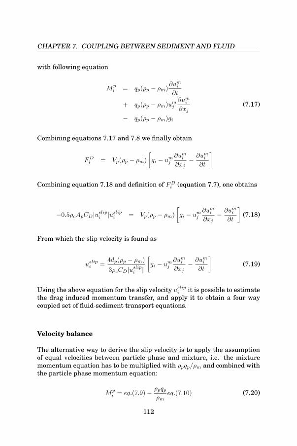
CHAPTER 7. COUPLING BETWEEN SEDIMENT AND FLUID
with following equation
Mpi = qp(ρp − ρm)
∂umi∂t
+ qp(ρp − ρm)umj∂umi∂xj
(7.17)
− qp(ρp − ρm)gi
Combining equations 7.17 and 7.8 we finally obtain
FDi = Vp(ρp − ρm)
[gi − umj
∂umi∂xj
− ∂umi∂t
]
Combining equation 7.18 and definition of FDi (equation 7.7), one obtains
−0.5ρcApCD|uslipi |uslipi = Vp(ρp − ρm)
[gi − umj
∂umi∂xj
− ∂umi∂t
](7.18)
From which the slip velocity is found as
uslipi =4dp(ρp − ρm)
3ρcCD|uslipi |
[gi − umj
∂umi∂xj
− ∂umi∂t
](7.19)
Using the above equation for the slip velocity uslipi it is possible to estimatethe drag induced momentum transfer, and apply it to obtain a four waycoupled set of fluid-sediment transport equations.
Velocity balance
The alternative way to derive the slip velocity is to apply the assumptionof equal velocities between particle phase and mixture, i.e. the mixturemomentum equation has to be multiplied with ρpqp/ρm and combined withthe particle phase momentum equation:
Mpi = eq.(7.9)− ρpqp
ρmeq.(7.10) (7.20)
112

CHAPTER 7. COUPLING BETWEEN SEDIMENT AND FLUID
As a result of combining equation 7.9 and 7.10 we obtain the followingequation for Mp
Mpi = qpρp
∂upi∂t− qpρp
ρmρm
∂umi∂t
+ qp∂pp∂xi− qpρp
ρm
∂pm∂xi
(7.21)
− ∂
∂xj[qp(τ
pij + τTpij )] +
qpρpρm
∂
∂xj
[τmij + τTmij + τDmij
]− qpρpgi +
qpρpρm
ρmgi
As it is possible to notice, basing on the applied assumption of equal veloc-ities, the convective terms have immediately been cancelled out. Applyingthe local equilibrium approximation, the diffusion drift velocity becomeszero, i.e. the first term in equation 7.21 cancels out. The viscous and tur-bulent stresses are assumed to be negligible, see the previous section (i.e.the pressure based method). Applying all above assumptions to the equa-tion 7.21 results in
Mpi = qp
∂pp∂xi− qpρp
ρm
∂pm∂xi
(7.22)
Assuming that pp ≈ pm and simplifying the above equation, results in
Mpi = qp
(ρm − ρp)ρm
∂p
∂xi(7.23)
Combining equations 7.23 and 7.8 we obtain following equation
−0.5ρcApCD|uslipi |uslipi = Vp
ρm − ρpρm
∂p
∂xi(7.24)
from which the slip velocity is found as
uslipi = −4
3
dp
ρcCD|uslipi |ρm − ρpρm
∂p
∂xi(7.25)
Set of slip velocity based, coupled, multiphase transport equations
Finally, the set of mixture transport equations is given by
∂ρm∂t
+∂ρmu
mi
∂xj= 0 (7.26)
113

CHAPTER 7. COUPLING BETWEEN SEDIMENT AND FLUID
∂ρmumi
∂t+∂ρmu
mi u
mj
∂xj= −∂pm
∂xi− ∂
∂xjτDmij +
∂
∂xjτGmij + ρmgi (7.27)
where τGmij is the sum of the viscous and turbulent mixture stresses and isdefined as
τGmij = (µ+ µTm)
[∂ui∂xj
+∂uj∂xi
](7.28)
The diffusion stress is defined as τDmij = ρmqp(1 − qp)|uslipi |uslipi . The dif-
fusion stress term is obtained by using the definition of drift velocity andassuming only one dispersed phase in equation 7.11.The continuity equation for the dispersed phase is given by
∂ρpqp∂t
+∂ρpqpu
mi
∂xj=
∂
∂xj(ρpqp(1−
ρpqpρm
)uslipi ) +∂
∂xjDMpij
∂qp∂xj
(7.29)
where (1 − qp)uslipi is the diffusion velocity expressed in terms of the slipvelocity, DMp
ij is the diffusion term. There are few models for that term incase of a RANS approach, e.g. the model suggested by Picart et al. (1986)which is defined as
DMpij = µ+ µTij
(1 + 0.85
(uslipi )2
2k/3
)−1/2
(7.30)
As it has been suggested by Manninen et al. [84], this RANS model givesthe best results for simulations with small particles, which follow well thefluid motions.However, in the LES framework the sediment fluxes are resolved to a largeextent (except for the subgrid scale fluxes). To model the subgrid scale sed-iment fluxes a proper subgrid scale model must be applied. Additionally,appropriate equations for CD and µm varying in function of concentrationshould be considered.All models presented in this section impose the two-way coupling betweenfluid and particle phase. However, as a result of the taken assumptionsthey are mainly valid for low concentrated suspensions of small particles.
7.5 SummaryThe theory presented in this chapter is just a short overview of the ex-isting literature. There exist more coupling approaches, settling velocitytheories or varying viscosity definitions. However, in this chapter only thebest known and important theories have been presented. In general, thecoupling between fluid and sediment is very complicated. First of all, what
114

CHAPTER 7. COUPLING BETWEEN SEDIMENT AND FLUID
usually is assumed (i.e. uniform sand size) practically can never be foundin natural conditions. In all kind of flows, e.g. rivers, many types of sed-iment can be found - from clay up to large sand particles. The influenceof such sediment composition on the flow field is much more complicatedthan it could be expected. Clay suspension has a big influence on the fluidviscosity, sand is changing the mixture density, which has an effect onthe momentum forces of the mixture, density and also viscosity. Fine andcoarse sand, gravel, small and bigger stones influence flow directly. Theyare changing the direction of the flow and they are also responsible for thegeneration of turbulent flow fluctuations (e.g. Von Karman street). Finallythey are also modifying the bottom roughness. It seems to be impossible tobuild one compact theory that would address all these processes at once. Itseems, that for the time being it is impossible to perform Direct NumericalSimulation of the effect of the clay influence on the flow including sand andgravel effects. This means that in order to obtain an accurate solution tothe mixture simulation, it will be necessary to build very complex modelswhich will also be based on empirical equations for sediment transport andits flow influence. One of the best solutions for sediment transport seemsto be the Large Eddy Simulation, where part of the flow is modeled (e.g.sgs scales, clay influence, clay coupling effects, etc.) and part is resolved(e.g. turbulence and its generation behind sand and gravel).There are several advantages of large eddy simulation compared to othercomputational methods. The large eddy simulation method offers a verygood balance between solution accuracy and computation speed. The meshesused for simulation can be relatively coarse. In LES the turbulent scalesare mostly resolved, and only a small part of them has to be modeled. Itis relatively easy to implement any empirical coupling equations. For allthese reasons, the LES methodology seems to be the best tool to studysediment transport and its influence on the flow in the near future.
115

CHAPTER 7. COUPLING BETWEEN SEDIMENT AND FLUID
116

Chapter 8
Application 3 -Investigation on sedimentand fluid coupling,standard methodologies
Contents8.1 Introduction . . . . . . . . . . . . . . . . . . . . . . . . . 1188.2 Description of the test cases . . . . . . . . . . . . . . . 1198.3 Carrier flow results . . . . . . . . . . . . . . . . . . . . . 1208.4 Sediment transport results . . . . . . . . . . . . . . . . 1268.5 Test case summary . . . . . . . . . . . . . . . . . . . . . 135
In the present chapter the influence of the sediment-fluid coupling is stud-ied. The sediment phase is considered in the Eulerian approach. Firstly,a thorough numerical investigation of the smooth bottom channel flow atReτ = 180 is performed using Large-Eddy Simulations (LES). A dynamicversion of the Wall Adapted Local Eddy-viscosity (WALE) model is used forthis study, whereas the sgs diffusion stress is based on a gradient hypothe-sis. The computed results compare well with Direct Numerical Simulation(DNS) data. Sediment-fluid coupling is obtained due to modification of vis-cosity, and, due to settling velocity modification, both models are based onthe sediment concentration, i.e. four way coupling has been used. It wasfound that the sediment has a strong influence on the flow field, also, inconcentrations as small as 1%. Assuming similar sediment concentration,
117

CHAPTER 8. APPLICATION 3 - INVESTIGATION ON SEDIMENTAND FLUID COUPLING, STANDARD METHODOLOGIES
it is shown that the influence of light sediment on flow conditions is smallerthan in case of heavier sand.
8.1 Introduction
Most sedimentation studies focus on the simplest case, where the sedi-ment particles are small, sediment concentration is small and the effectsof the sediment-fluid and sediment-sediment interaction are neglected, i.e.Cabot and Moin [18], Widera et al. [153] or Widera et al. [152] and manyothers. In above mentioned cases only undisturbed flow or bottom rough-ness influence on transport of low concentrated sediment has been inves-tigated. However, it seems that coupling between sediment and fluid, andbetween sediment and sediment might play an important role in the pro-cess of the sediment transport. It is known that many sediments tends tosettle in the near wall region, e.g. sand particles, also this kind of sedimentis considered in the manuscript. The increase of the sediment concentra-tion towards the bottom is a natural consequence of the effect of gravity onthe suspended particles. This process can influence the bottom roughnessor the near bottom fluid viscosity and can disturb the near wall flow layerand also, further on, the developed flow region. In the present chapter aninvestigation of the influence of the sediment-fluid, and sediment-sedimentcoupling on the flow and on the sediment transport patterns is presented.The sediment-fluid coupling is obtained using a varying viscosity model,where the viscosity of the fluid is changing proportionally to the sedi-ment concentration, see model of Toda and Hisamoto [131]. The sediment-sediment coupling is based on an empirical equation derived by Van Rijn[148]. The equation proposed by Van Rijn has been obtained through de-tailed experimental investigation. In the model of Van Rijn [148] the sedi-ment settling velocity is also varying as a function of sediment concentra-tion. Because of the coupling of all phases, the results presented in thismanuscript are obtained from a fully coupled simulation, i.e. a four waycoupling is applied.
The Chapter is organized as follows. In section 2, the considered test casesare described. The carrier flow results are discussed in section 3. In section4, solution and description of sediment results are presented. Conclusionsare given in section 5.
118

CHAPTER 8. APPLICATION 3 - INVESTIGATION ON SEDIMENTAND FLUID COUPLING, STANDARD METHODOLOGIES
8.2 Description of the test cases
A series of five cases is considered. They all deal with the flow with sus-pended sediment in a closed channel. Periodic boundary conditions are im-posed in the streamwise and spanwise directions. At the upper and lowerwall a no-slip boundary condition is imposed. The channel dimensions are0.24m × 0.04m × 0.12m with 64 × 64 × 64 cells resp. in streamwise, verti-cal and spanwise direction. The nondimensional cell size are: 4x+ = 33and 4z+ = 11. The cell size in the vertical direction is varying between4y+ = 0.5 near the wall and 4y+ = 14 in the channel center.
The presented cases can be divided into three main groups. In the firstcase, the influence of varying viscosity is shown and described. The viscos-ity coupling is based on model of Toda and Hisamoto [131], see equation7.5. of This set of cases is treated as a reference for the other simulations.In the second set of simulations, the sediment concentration is kept iden-tical as in the reference group, but the particle diameter is equal to 50%of the particle diameter from the reference case. The third set of simula-tions considers the same particle diameter as in the reference set, but thesediment concentration is doubled. The settling velocity of the sediment isvarying according to model proposed by Van Rijn [148], see equation 4.36.The sediment settling velocity has been calculated basing on the Stokesequation. To account for sediment-sediment coupling, the varying settlingvelocity model of Van Rijn has been used, see equation 4.36.
To give an overview of the simulation conditions, the most important set-tings are summarized in Table 1.
Table 8.1: Summary of test cases
Case µ dp[mm] qini %C1 constant 0.06 1%C2 varying 0.06 1%C3 varying 0.03 1%C4 varying 0.06 2%C5 constant 0.06 2%
The boundary conditions for the sediment equation at the bottom and topsurface are based on the zero flux condition, and they are defined similarlyas in previous applications, see equation 5.3 or Appendix, equation 10.39to 10.52.
119

CHAPTER 8. APPLICATION 3 - INVESTIGATION ON SEDIMENTAND FLUID COUPLING, STANDARD METHODOLOGIES
8.3 Carrier flow resultsIn the present section the study of the flow solution is presented. CasesC1 and C2 are treated as a reference for cases C3, C4 and C5. Figures, 8.1up 8.3 present a comparison of the velocity profiles obtained with LES (fordifferent settings) with those from Direct Numerical Simulation (DNS) ofuncoupled flow with Reτ = 180 performed by Moser et al. [96]. The lefthand side plots present the velocity in nondimensionalised form with lin-ear ordinate and logarithmic abscissa. The right hand side plots presentnondimensionalised velocities on a double logarithmic plot to increase plotclarity in the near wall region.
(a) (b)
Figure 8.1: Time and space averaged velocity, (a) linear-logarithmic scale, (b)logarithmic-logarithmic scale
Figure 8.1 presents the solution for the case of sediment transport withand without varying viscosity model. Comparing these solutions, it be-comes clear, that the varying viscosity model has a relatively big ∗ impacton the flow field solution, especially in the viscous sub-layer. This is aneffect of the settling process. Sediments transported in channels, tend tosettle (due to gravitational acceleration) and concentrate in the near bot-tom region. This means, that the sediment concentration near the wall willbecome much higher than the mean concentration in the domain †. Thus,the highly increased sediment concentration in the near wall region can
∗It has to be taken under account that volumetric concentration of the sediment is 1%only†Difference in concentration between top and bottom of the channel can reach even sev-
eral orders of magnitude.
120

CHAPTER 8. APPLICATION 3 - INVESTIGATION ON SEDIMENTAND FLUID COUPLING, STANDARD METHODOLOGIES
substantially affect the viscosity of the sediment-fluid mixture. Because inboth cases the friction velocity is the same, and the fluid viscosity is rising,therefore, the near wall fluid velocity is decreasing, which partially affectsthe rest of the flow field.
(a) (b)
Figure 8.2: Time and space averaged velocity, (a) linear-logarithmic scale, (b)logarithmic-logarithmic scale
Figure 8.2 presents a comparison between the reference cases (C1 and C2)and a case with similar settings, but with two times smaller particle di-ameter, case C3. As it can be seen, the influence of the sediment to theflow solution in case of smaller particles are practically negligible. This, iscaused mainly by the very small influence of the particles on the viscosity.Since the imposed particle diameter is smaller than the particle from caseC1 and C2, its settling velocity is also smaller. Thus, due to lower settlingvelocity of particles, they do not concentrate in the near wall region asmuch as the heavy particles (case C1 and C2). Hence, the viscosity changeis negligible, and viscous coupling has no influence on the flow solution.
The comparison of cases C1, C2 and C4 is shown in figure 8.3. The differ-ence between the solution of low and high concentrated suspension (2%)is clear. As it can be expected the increased sediment concentration has alarger influence on the flow than the lower concentrated suspension, seefigure 8.3(b).
The influence of the sediment concentration can be very clearly presentedby the velocity gradient profiles. Figure 8.4(a) up to figure 8.4(d) presenta comparison of the velocity gradient profiles in case C1 and cases C2, C3,C4 and C5. It is easy to notice that the profiles of the velocity gradient in
121

CHAPTER 8. APPLICATION 3 - INVESTIGATION ON SEDIMENTAND FLUID COUPLING, STANDARD METHODOLOGIES
(a) (b)
Figure 8.3: Time and space averaged velocity, (a) linear-logarithmic scale, (b)logarithmic-logarithmic scale
cases with constant viscosity are symmetrical with respect to the channelsymmetry axis (y/h = 0.5), while for cases with varying viscosity, the pro-files are unsymmetrical, i.e. in case C2, C3 and C4.
The zoom of the velocity gradient in the near wall region is shown in figure8.5. The strong influence of the viscosity coupling on the fluid velocityprofiles can be observed. The largest drop of the velocity gradient can benoticed in figure 8.5(c), with results of case C4, where the concentrationof the sediment is 2%. Comparing this profile with the undisturbed profileof case C1 it is possible to estimate the difference, which is about 40%.This result gives an idea, of how drastically the flow field is disturbed withsuch a small sediment concentration. A very similar result is obtainedcomparing the solution C1 to C2, figure 8.5(a). The difference between thevelocity gradients reaches more than 30%, which is rather big, especiallytaking into account that the volumetric concentration of the sediment wasonly 1%.However, comparing figures 8.5(a) and 8.5(c), it is possible to notice that incase C2 at the upper surface, the near wall layer is practically undisturbed,while in case C4 there is a clear drop of the velocity gradient. In case C3,see figure 8.5(b) the top near wall velocity gradient profile is unaffected,while the drop of the velocity gradient in the bottom region is less than10%. This is caused by much a more even dispersion of sediment particlesin the flow. Again, this is due to the smaller particle size, thus, smallersettling velocity.While the effect of viscosity coupling is not very well visible on the aver-
122

CHAPTER 8. APPLICATION 3 - INVESTIGATION ON SEDIMENTAND FLUID COUPLING, STANDARD METHODOLOGIES
(a) (b)
(c) (d)
Figure 8.4: Gradient of the averaged velocity in vertical direction.
aged velocity plots, it is very noticeable in the results for the velocity fluc-tuations. Figures 8.6 to 8.9 present results of streamwise, spanwise andhorizontal root mean square (rms) of velocity fluctuations. Additionally,the Reynolds stresses are presented. As for the averaged velocity profiles,the rms results obtained with LES are compared with DNS solution.However, the comparison between the rms velocities obtained from DNSand LES presented in figures 8.6 to 8.9 is not entirely valid. For detaileddescription please see 3.4.4 or Winckelmans et al. [155].As it can be noticed, the velocity fluctuations in cases with viscosity cou-pling always increase, mainly in the lower part of the channel. This showsand confirms the influence of the sediment phase on the fluid. The higherlevel of fluid velocity fluctuations can be explained by the increased, thelow speed, near wall layer. This creates a larger area of mixing betweenthe developed layer and the viscous sublayer. Hence, the turbulence level
123

CHAPTER 8. APPLICATION 3 - INVESTIGATION ON SEDIMENTAND FLUID COUPLING, STANDARD METHODOLOGIES
(a) (b)
(c) (d)
Figure 8.5: Gradient of the averaged velocity in vertical direction. Zoom of the nearwall region.
is increased. A large impact of the near bottom sediment concentration canbe noticed very clearly in cases C2 and C4. The difference in rms valuesbetween the coupled and uncoupled case is about 6% in case C2 and 7% incase C4.
The case C3, where a concentration similar to the case C2 has been consid-ered, is presented in figure 8.7. It is possible to notice, that the influence ofthe smaller sediment size is very small. Due to the more uniform disper-sion of the sediment phase across the wall normal direction, the flow fieldis barely affected by changes of the fluid viscosity.
Additionally, it is interesting to note that based on the present results, it isvery clear that sediment-fluid coupling has a very strong influence on thesymmetry of the rms profiles with respect to half of the channel height.
124

CHAPTER 8. APPLICATION 3 - INVESTIGATION ON SEDIMENTAND FLUID COUPLING, STANDARD METHODOLOGIES
(a) (b)
(c) (d)
Figure 8.6: The rms of the velocity fluctuations, case C1-C2.
The difference in symmetry is most clear in cases where large particlesare considered, this can be seen in figures 8.6 and 8.8. Velocity fluctuationprofiles are changing in the same manner, in each case, i.e. C1, C3, C4.The only difference is in amplitude. However, as it is possible to expect,the rate of change depends mainly on the particle size and particle concen-tration.
Very interesting insight into the change of the mixture viscosity can be no-ticed in figure 8.10, where the ratio of the mixture and clear fluid viscosityare shown. As it is possible to notice the change of the mixture viscosityis the lowest in the situation when light particles are used, i.e. case C3,see figure 8.10(b). In this case, the near bottom mixture viscosity increasesabout 7%, comparing to the uncoupled solution. In case C2, the mixtureviscosity is increased for about 35%. As it is expected, the highest increaseof the mixture viscosity in the near wall region can be noticed in figure
125

CHAPTER 8. APPLICATION 3 - INVESTIGATION ON SEDIMENTAND FLUID COUPLING, STANDARD METHODOLOGIES
(a) (b)
(c) (d)
Figure 8.7: The rms of the velocity fluctuations, case C1-C3.
8.10(d) which present solution for case C4.Figures 8.11 and 8.12 present the sgs model coefficient profiles along thewall normal direction. As it can be noticed, the influence of the sediment-fluid viscosity based coupling on the subgridscale model coefficient is neg-ligible.
8.4 Sediment transport resultsIn the present section the sediment transport results are presented. Atfirst sediment concentration profiles will be shown. Next, the sedimentfluxes will presented.Figure 8.13 presents sediment concentration profiles for all consideredcases, i.e. C1, C2, C3, C4 and C5. As it is possible to notice, the sediment-fluid coupling does not influence remarkably the sediment concentrationprofiles. The only visible changes could be noticed in the near wall region,
126

CHAPTER 8. APPLICATION 3 - INVESTIGATION ON SEDIMENTAND FLUID COUPLING, STANDARD METHODOLOGIES
(a) (b)
(c) (d)
Figure 8.8: The rms of the velocity fluctuations, case C1-C4.
where in the case of viscous coupling (see figure 8.13(a) and 8.13(c) the ve-locity profile is substantially disturbed.
As it is possible to notice in figure 8.13(b), the sediment concentration pro-file for case C3 is very steep comparing to concentration profile for case C1.The high concentration steepness for case C3 is an effect of the lower set-tling velocity of smaller particles. Because of the lower settling velocity, thesediment concentration across the channel hight in case C3 is more uni-form than in case of heavier (or/and larger) particles, i.e. in all other cases.As it can be seen, the sediment concentration profile of heavier particles(case C1) is spread over three orders of magnitude, while the concentrationprofile of small particles (case C3) is spread over one order of magnitudeonly, see figure 8.13(b).
Figures 8.14 and 8.15 present a comparison of the sediment flux profiles
127

CHAPTER 8. APPLICATION 3 - INVESTIGATION ON SEDIMENTAND FLUID COUPLING, STANDARD METHODOLOGIES
(a) (b)
(c) (d)
Figure 8.9: The rms of the velocity fluctuations, case C1-C5.
in streamwise and vertical direction. As expected, the particle flux in thecases with varying viscosity is higher than that in case of constant viscos-ity. This effect can be explained by the increased viscosity of the fluid incase of the varying µ. Because of the increased mixture viscosity the par-ticle needs less upward velocity to be kept in suspension. Additionally, theparticle can better follow fluid motions.
A substantial difference in the sediment flux, (about one order of magni-tude), can be observed comparing reference case (C1) and the case withsmaller particles (C3), see figure 8.14(b) and 8.15(b). The explanation forthis large difference is that, smaller particles follow the fluid motions muchbetter than heavy ones, and therefore they are more uniformly distributedacross the channel.
In case of the same particle size, when comparing low (C1, C2) with higher
128

CHAPTER 8. APPLICATION 3 - INVESTIGATION ON SEDIMENTAND FLUID COUPLING, STANDARD METHODOLOGIES
(a) (b)
(c) (d)
Figure 8.10: Ratio of the clear fluid viscosity to the mixture viscosity.
(C4, C5) concentration, the sediment fluxes are much closer to each other,as it is shown in figure 8.14(a),8.14(d) and 8.15(a),8.15(d). The differencein streamwise flux amplitude is about 20% between cases C1 and C2, andabout 30% for case C4−C5. While, the difference in flux amplitude in verti-cal direction is about 10% in case of low concentrated suspension (C1−C2),and 18% for high concentrated case (C4− C5).
129

CHAPTER 8. APPLICATION 3 - INVESTIGATION ON SEDIMENTAND FLUID COUPLING, STANDARD METHODOLOGIES
(a) (b)
(c) (d)
Figure 8.11: Comparison of the sgs model coefficient in the wall normal direction,fluid phase
130

CHAPTER 8. APPLICATION 3 - INVESTIGATION ON SEDIMENTAND FLUID COUPLING, STANDARD METHODOLOGIES
(a) (b)
(c) (d)
Figure 8.12: Comparison of the sgs model coefficient in the wall normal direction,sediment phase
131

CHAPTER 8. APPLICATION 3 - INVESTIGATION ON SEDIMENTAND FLUID COUPLING, STANDARD METHODOLOGIES
(a) (b)
(c) (d)
Figure 8.13: Sediment concentration profiles.
132
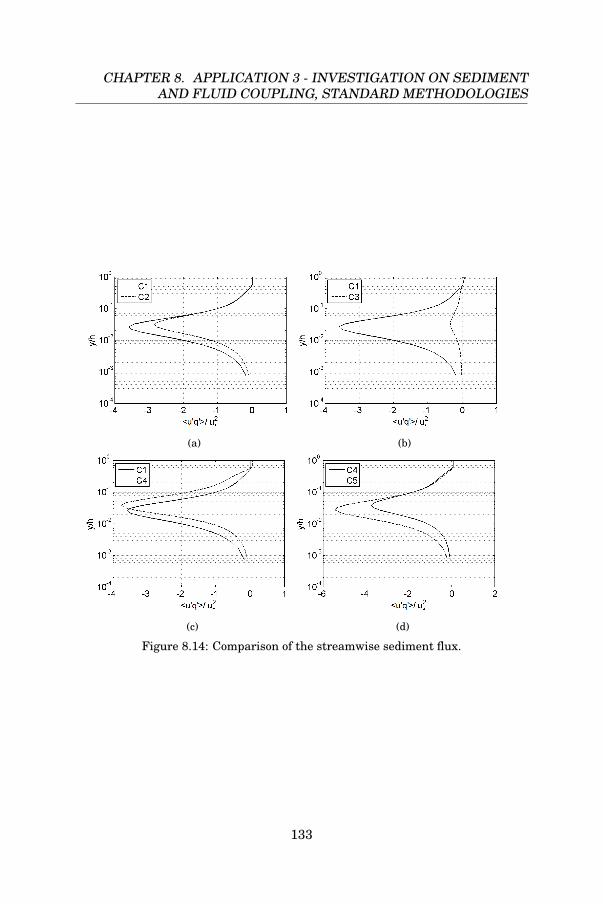
CHAPTER 8. APPLICATION 3 - INVESTIGATION ON SEDIMENTAND FLUID COUPLING, STANDARD METHODOLOGIES
(a) (b)
(c) (d)
Figure 8.14: Comparison of the streamwise sediment flux.
133

CHAPTER 8. APPLICATION 3 - INVESTIGATION ON SEDIMENTAND FLUID COUPLING, STANDARD METHODOLOGIES
(a) (b)
(c) (d)
Figure 8.15: Comparison of the vertical sediment flux.
134

CHAPTER 8. APPLICATION 3 - INVESTIGATION ON SEDIMENTAND FLUID COUPLING, STANDARD METHODOLOGIES
8.5 Test case summaryThe effect of particle-fluid coupling has been investigated. It is found thatthe influence of the sediment on the flow can be noticed also for very smallconcentrations. This is due to the increased sediment concentration in thenear wall region, which at a certain level considerably changes the mix-ture viscosity. It has also been found that lighter particles have consider-ably less effect on the flow as compared to larger particles. This is becausethe smaller particles do not concentrate in the near bottom region to thesame extent as the heavier particles. As a result the near wall layer is lessaffected by the viscosity change, and the rest of the flow is also practicallyundisturbed. It should be noted here, that because of the low Reynoldsnumber flow, the transported particles are very small. The size of the sed-iment which is considered in the manuscript has been chosen because ofthe low capacity of the flow turbulence to suspend heavier particles. It ispossible that if larger particles would be used their influence to the flow,assuming similar concentration, would also be considerably bigger.
135

CHAPTER 8. APPLICATION 3 - INVESTIGATION ON SEDIMENTAND FLUID COUPLING, STANDARD METHODOLOGIES
136

Chapter 9
Application 4 -Investigation on sedimentand fluid coupling, thedrift flux model
Contents9.1 Introduction . . . . . . . . . . . . . . . . . . . . . . . . . 1389.2 Description of the test cases . . . . . . . . . . . . . . . 1399.3 Carrier flow results . . . . . . . . . . . . . . . . . . . . . 1409.4 Test case summary . . . . . . . . . . . . . . . . . . . . . 151
Large Eddy Simulation (LES) is used to investigate drift flux models, whereone is based on the pressure and the second one is based on the velocityfield. The WALE (Wall-Adapting Local Eddy-viscosity) model is used formodeling the subgrid scale fluid stresses. To avoid tuning constants, thedynamic procedure has been applied. Slip velocity results are comparedand validated against Direct Numerical Simulation (DNS) solution of par-ticle transport in channel flow without gravity with Re = 150∗. The par-ticle transport model used in DNS of Marchioli et al. [85] is based on theLagrangian approach. The particle size considered, expressed as a Stokesnumber, is ranging from St = 0.2† to St = 15. The obtained results are in∗Reynolds number is defined as Reτ = u∗h/ν, where u∗ =
√τw/ρf is the friction (or
shear) velocity, τw is the mean shear stress at the wall, ρf is the clear fluid density, h is thehalf channel height and ν is fluid kinematic viscosity.†Particle Stokes number is defined as St = τpu2∗, where τp = (d2pρp)/(18µ), dp is the
137

CHAPTER 9. APPLICATION 4 - INVESTIGATION ON SEDIMENTAND FLUID COUPLING, THE DRIFT FLUX MODEL
good correspondence with slip velocities of the particles obtained from sim-ulation based on the Lagrangian approach. However, there is also a con-siderable difference between the two investigated Eulerian models. Thus,the most common assumption that both models give similar results seemsto be erroneous.
9.1 IntroductionThe transport of particles under any form, e.g. as dust, as inhaled medicines,as transport of sand in rivers, channels or piping systems is one of the mostimportant and at the same time, one of the least understood phenomenathat we are confronted with. Up till now, the proper tools to understandthese processes are still lacking. There are multiple ways to investigateissues related to particle transport; they can be based on measurements,theoretical and/or on numerical considerations. One of the fastest grow-ing means to investigate problems of particle transport in everyday lifeis Computational Fluid Dynamics (CFD). CFD methods for the simula-tions of flows with particles can be based on a Lagrangian approach or onan Eulerian methodology. Whereas the Lagrangian methodology is suit-able for e.g. the simulations of medical particle dispersion in lungs, it israther unpractical (from the computational time point of view) to applythis methodology in transport of sand particles in, e.g. rivers, estuaries orlarge, industrial piping systems, where the number of particles is in prac-tice uncountable. In such applications one has to resort to an Eulerianapproach, where the particle phase is considered as a continuum, exactlyin the same way as the carrying fluid. The advantage of this method isits computing time, which is always the same, independently of the par-ticle concentration. Unfortunately, in the Eulerian methodology it is notpossible or rather very difficult to apply any changes to influence motionpattern of particles. However, in 1984, Ishii and Mishima [64] proposeda model for the momentum induced transfer between phases within anEulerian framework. Basing on that work, Manninen et al. [84] in 1996presented a mathematical derivation of the particle slip velocity based onthe Eulerian mixture equations. Manninen et al. [84] presented basicallytwo models to calculate the particle slip velocity, one is based on the pres-sure field and the second one is based on the velocity field. They claim thatboth models should give similar results, since they were derived basing onthe same assumptions and approximations. Since Manninen et al. [84]proposed their models, several papers have been published where authorswere presenting results of the particle transport using one of the slip mod-
particle diameter, ρp is the particle density and µ is the fluid dynamic viscosity.
138

CHAPTER 9. APPLICATION 4 - INVESTIGATION ON SEDIMENTAND FLUID COUPLING, THE DRIFT FLUX MODEL
els, e.g. Longest and Oldham [82]. In the present work, both models willbe compared and verified against DNS results of Marchioli et al. [85], whoperformed simulations of a particle transport in a vertical channel usingthe Lagrangian approach.
9.2 Description of the test casesThe testcase used is based on the closed channel flow with Reτ = u∗h/ν =150, where u∗ is the friction velocity, h is the channel half height, and theν is the fluid kinematic viscosity of the air. Standard air conditions areconsidered. The mesh cell size is kept constant in the streamwise andspanwise direction, while it has been refined symmetrically towards bothwalls. Three meshes are used, all of the same dimensions, but differing innumber of cells. The coarsest mesh consists of 33× 33× 33 cells in i× j × kdirections, respectively. The medium mesh consists of 48×48×48 cells andthe fine mesh of 64 × 64 × 64 cells. The three different mesh resolutionswere used to estimate the influence of the cell size on the accuracy of theslip velocity models. The nondimensional cell sizes for the three meshesare, 4x+ = (4xu∗)/ν = 54, 4y+
max = 24, 4z+ = 19 for the coarse mesh,4x+ = 37, 4y+
max = 17, 4z+ = 13 and 4x+ = 28, 4y+max = 11, 4z+ = 10
for medium and fine mesh, respectively. The stretching towards wall andfree surface is performed according to the following equations
y = (1/g ∗ tanh(ψ ∗ ξ) + 1) ∗ 0.06 (9.1)
where ψ = −1 + (NY − 1)/32, ξ = log((1 + g)/(1 − g))/2, g = 0.96846 andNY is the cell number in the y direction.
To study properties of slip velocity models proposed by Manninnen et al.[84] five numerical simulations have been performed, see Table 9.1 for anoverview. There are two main simulations, referred to as M1 and M2,which are based on velocity (see equation 7.19) and pressure (see equa-tion 7.25) approach (test cases M1 and M2, respectively). In these cases,the universal drag approach proposed by Schiller and Naumann has beenapplied, see equation 4.10 or [119] for more information. In case M3 theVan Driest type damping function has been taken into account. In casesM4 and M5 the Stokes drag function is applied. Since the velocity basedmodel is underestimating the slip velocity, it does not need the dampingfunction. Hence, the Van Driest damping has been applied only to thepressure based model.Four particle sets were considered in presented simulations. They arecharacterized by different relaxation time τp = ρpd
2p/18µ. Their Stokes
139

CHAPTER 9. APPLICATION 4 - INVESTIGATION ON SEDIMENTAND FLUID COUPLING, THE DRIFT FLUX MODEL
Table 9.1: Summary of test cases
run slip model drag model Van Driest dampingM1 velocity based Schiller & Naumann NoM2 pressure based Schiller & Naumann NoM3 pressure based Schiller & Naumann YesM4 pressure based Stokes NoM5 velocity based Stokes No
number value St = (τpu2∗)/ν is between 0.2 and 15. Table 9.2 shows the
basic parameters of the considered particles.
Table 9.2: Particle parameters
Stokes number τp[s] dp[µm] ρp[kg/m3]
0.2 1.67× 10⁻⁴ 9 7001 8.26× 10⁻⁴ 20 7005 4.18× 10⁻³ 45 70015 1.26× 10⁻² 78 700
9.3 Carrier flow resultsThe present section is divided into two subsections. In the first part resultsobtained from the simulations are compared with reference data from theliterature to validate the fluid flow solver. In the second part, the slip ve-locity characteristics are investigated.
To evaluate the accuracy of the flow solver the first and the second orderflow statistics are compared. The flow statistics are compared to DNS dataof flow with Reτ = 180 of Moser et al. [96].
Figure 9.1 presents a comparison between the nondimensionalized veloc-ity profiles along the wall normal direction obtained with LES with thoseof DNS. The profiles obtained using LES are in good agreement with DNSdata. It is possible to notice that refinement of the mesh increases the ac-curacy of the LES model, as expected. However, the comparison betweenthe rms velocities obtained from DNS and LES presented in figure 9.2 isnot entirely valid. For detailed description please see 3.4.4 or Winckel-mans et al. [155].
140

CHAPTER 9. APPLICATION 4 - INVESTIGATION ON SEDIMENTAND FLUID COUPLING, THE DRIFT FLUX MODEL
Figure 9.1: Comparison between model M2 and M3.
Figure 9.2 presents the comparison of the second order flow statistics. Asfor the first order statistics, it is observed that mesh refinement improvesthe accuracy. It can be noticed that the accuracy of the dynamic WALEmodel brings the solution very close to the DNS one, even in case withcoarsest mesh, while the difference between LES and DNS in case withfine mesh is practically negligible, e.g. for rms of the streamwise velocityfluctuation and Reynolds stresses.
Slip velocity resultsIn the present section the slip velocity results are presented. There are twoslip velocity models that are considered. One calculates the particle phaseslip velocity based on the instantaneous velocity field, this model is re-ferred to as the velocity based model, see equation 7.19, The other model,that is based on the pressure field, is referred to as the pressure basedmodel, see equation 7.25. For more detailed description of these modelsplease refer to the section 7.4 or to the Manninen et al. [84] report.
As first, the comparison of both models to the DNS solution of Marchi-oli et al. [85] will be presented. Additional information about that testcase can also be found in Picciotto et al. [108].
Results obtained with the slip velocity models are compared to the DNSsolution of Marchioli et al. [85] to validate the accuracy of the models pro-posed by Manninen et al. [84]. The data presented by Marchioli et al. [85]
141

CHAPTER 9. APPLICATION 4 - INVESTIGATION ON SEDIMENTAND FLUID COUPLING, THE DRIFT FLUX MODEL
(a) (b)
(c) (d)Figure 9.2: Comparison between LES and DNS results. Figure presents followingresults: rms of the streamwise velocity fluctuations (top left), rms of the velocityfluctuations in vertical direction (top right), rms of the spanwise velocity fluctua-tions (bottom left) and the Reynolds stress (bottom right)
seems to be most relevant for this purpose. Firstly, there is no influence ofany turbulence model, which makes the flow field results free of any mod-eling errors. Secondly, the particle motion equation used by Marchioli etal. [85] is also based on the drag force. Hence, considering the forces ap-plied to the sediment phase, both, i.e. the Lagrangian model of Marchioliet al. [85] and the Eulerian approach proposed by Manninen et al. [84] aresimilar from the point of view of the definition of the particle motion.
Figures 9.3 and 9.4 show the comparison between the slip velocities forfour particle sizes, where on each plot the results of the LES simulation onthe three different meshes are presented. Figure 9.3 presents the solutionof the velocity based model and figure 9.4 from the pressure based model.
142

CHAPTER 9. APPLICATION 4 - INVESTIGATION ON SEDIMENTAND FLUID COUPLING, THE DRIFT FLUX MODEL
This test has been performed to check the influence of the mesh refinementon the accuracy of the slip velocity models. As it is visible, the velocitybased model gives a reasonably good accuracy for smaller particles, whilefor bigger particles it tends to overestimate the slip velocity.
(a) (b)
(c) (d)Figure 9.3: Investigation on the model accuracy based on the mesh resolution,for velocity based model - model 1. The particle Reynolds number is defined asRep = |uslip|dp/ν where |uslip| is the particle slip velocity, dp particle diameter andν fluid viscosity.
It can also be observed that the shape of the particle Reynolds profile ob-tained with the velocity based slip model is flatter than the one of the DNSsolution. This means that the velocity based model is less responsive forthe change of the velocity fluctuation level across the channel height thanthe pressure based model or the DNS one, see figure 9.3 and 9.4.The second model, i.e. the pressure based model clearly underestimatesthe slip velocities for small particles, i.e. for the particles with St ≤ 1.However, the profile of the particle Reynolds number is very similar to the
143

CHAPTER 9. APPLICATION 4 - INVESTIGATION ON SEDIMENTAND FLUID COUPLING, THE DRIFT FLUX MODEL
(a) (b)
(c) (d)Figure 9.4: Investigation on the model accuracy based on the mesh resolution, forpressure based model - model 2.
one of DNS. As can be seen in figure 9.4, the pressure based model givesthe solution close to DNS only for bigger particles, i.e. where St ≥ 5.Figure 9.5 presents the comparison between the LES solution of both slipvelocity models with DNS. It can be observed that difference between bothLES models is almost independent of the particle size, e.g. the differ-ence between the two slip velocity models in the center of the channel(y/h ≈ 0.5) is practically the same for all particle sizes. The second dif-ference is in the near wall region (y/h ≈ 0.0), where the difference betweenthe velocity based model and the pressure one is substantial. It is clearthat the velocity based model underestimates the particle slip velocity nearthe wall, while the pressure based model overestimates it, see figure 9.5.
The settling overestimation of the pressure based model is very well visi-ble in the results presented by Longest and Oldham [82]. They presented
144

CHAPTER 9. APPLICATION 4 - INVESTIGATION ON SEDIMENTAND FLUID COUPLING, THE DRIFT FLUX MODEL
(a) (b)
(c) (d)Figure 9.5: Comparison between model M1 and M2.
solutions with three slip velocity models (all of them are pressure based)with the model differing in the treatment of the first cell near the wall.Longest and Oldham [82] proposed correction of the slip velocity in thefirst near wall cell. In the case of an uncorrected slip velocity model, theirresults show a very high overestimation of settling, i.e. the slip velocitywas greatly overestimated. With some corrections, the results presentedby Longest and Oldham [82] show a high accuracy comparing to the ex-periment. However, it is possible that the correction of the slip velocityin the cell nearest to the wall might not be enough. In order to damp theoverestimated slip velocity in the near wall region a Van Driest damping isproposed, instead of velocity correction in the first cell only. The modifiedVan Driest (DV D) damping model, see Piomelli et al. [111], is defined as
DV D =√
(1− exp(−y+/A+)3) (9.2)
A coefficient is changed to A+ = 4, instead of commonly used A+ = 25 in
145

CHAPTER 9. APPLICATION 4 - INVESTIGATION ON SEDIMENTAND FLUID COUPLING, THE DRIFT FLUX MODEL
the case of subgrid scale fluctuations in LES. The main advantage of thatmodel is its simplicity.Results of Van Driest damping are presented in figure 9.6 and in figure9.7. Figure 9.6 shows that damping of the slip velocity has no effect on themain behavior of the slip velocity model, i.e. there is no change in the par-ticle Reynolds profile between model M2 and M3, except in the near wallregion. The effect of the Van Driest damping on the particle slip velocitiesis well visible in figure 9.7, where the zoom of near wall part of the particleReynolds number profile is presented to better visualize the difference be-tween all three models and the DNS solution, i.e. 0.0 < y/h < 0.05 insteadof 0.0 < y/h < 0.05, as in figure 9.6. As it is possible to observe, apply-ing the damping function corrects the slip velocity profile. Unfortunately,the used damping function does not provide smooth transition betweencorrected and uncorrected parts of the slip velocity profile.
(a) (b)
(c) (d)Figure 9.6: Comparison between model M2 and M3.
146

CHAPTER 9. APPLICATION 4 - INVESTIGATION ON SEDIMENTAND FLUID COUPLING, THE DRIFT FLUX MODEL
(a) (b)
(c) (d)Figure 9.7: Comparison between Eulerian based slip models, where one model isbased on the velocity field and the second is based on the pressure field, whereone of the pressure models has been modified to account for a near wall layer ef-fects. The nondimensional particle size is: St=0.2 (top left), St=1 (top right), St=5(bottom left) and St=15 (bottom right).
Figures 9.8 and 9.9 present the comparison between the slip velocity mod-els based on a Stokes drag and those based on the Schiller and Naumann[119] formula. Figure 9.8 shows the solution of the pressure based modeland figure 9.9 of the velocity based model.One can easily notice that the difference in the drag has little effect on theslip velocity, except for larger particles where the use of the Schiller andNaumann [119] model gives results closer to DNS.Figure 9.10 presents the comparison between the particle Reynolds num-ber along the channel height obtained from LES (only pressure based modelis used) and DNS. Note that the LES results are Eulerian, whereas theDNS results are Lagrangian. In case of DNS the location of the peak in
147

CHAPTER 9. APPLICATION 4 - INVESTIGATION ON SEDIMENTAND FLUID COUPLING, THE DRIFT FLUX MODEL
(a) (b)
(c) (d)Figure 9.8: Comparison between model M2 and M4.
particle Reynolds number moving forward the wall with increasing parti-cle Stokes number.The LES results in contrast, predict the same location of the peak irre-spective of the particle size. This is an effect of the difference in calcu-lation of the slip velocities in the Lagrangian and Eulerian frameworks.In the Lagrangian methodology particle slip velocity is obtained based onparticle tracking, whereas in the Eulerian methodology the slip velocityis obtained based on the flow field solution, thus the peak in the particleReynolds number will always be at the same place.The solutions of both Eulerian slip velocity models for all particle sizesare presented in figure 9.11. For all particle sizes the obtained particleReynolds numbers are close to the Lagrangian DNS solution. This is asatisfactory result, especially if it is taken into account that the range ofthe particle Reynolds numbers that is covered, extends over four orders of
148

CHAPTER 9. APPLICATION 4 - INVESTIGATION ON SEDIMENTAND FLUID COUPLING, THE DRIFT FLUX MODEL
(a) (b)
(c) (d)Figure 9.9: Comparison between model M1 and M5.
magnitude. However, neglecting in both models for the laminar and theturbulent stresses does not seem to be correct, especially in the near walllayer where the viscous stresses are dominant. The lack of the laminarand turbulent stresses has a severe influence on the particle response tothe fluid velocity fluctuations, both, in the near wall and in the developedregion. Furthermore, neglecting all stresses in the pressure based mod-els results in uncorrect estimation of the drift velocity in the near wallregions. Hence, it can be stated that incorporating the laminar and turbu-lent stresses in the slip velocity models will improve their accuracy.
149

CHAPTER 9. APPLICATION 4 - INVESTIGATION ON SEDIMENTAND FLUID COUPLING, THE DRIFT FLUX MODEL
(a) (b)
Figure 9.10: Comparison between Eulerian and Lagrangian slip velocity profiles,the Eulerian models is based on the pressure field. Particle Reynolds number pro-files are scaled over their highest values. LES - Eulerian methodology (left), DNS- Lagrangian methodology (right).
Figure 9.11: The comparison of the slip velocities between DNS with Lagrangianmethodology and Eulerian approach where the pressure and velocity based modelshave been used, for particle Stokes number from St = 0.2 up to St = 15.
150

CHAPTER 9. APPLICATION 4 - INVESTIGATION ON SEDIMENTAND FLUID COUPLING, THE DRIFT FLUX MODEL
9.4 Test case summaryIn this chapter the results of two slip velocity models proposed by Manni-nen et al. [84] are presented. The results are obtained by the use of largeeddy simulation of the flow in a vertical channel, where the flow in stream-wise and spanwise direction is periodic. Results of LES simulation usingan Eulerian approach are compared to the DNS solution obtained with aLagrangian approach.
The obtained results confirm the validity of the underlying assumptionsand the procedure for deriving the slip velocity as proposed by Manninenet al. [84]. The velocity based model gives relatively accurate solution forsmaller particles, i.e. St ≤ 1 and has a tendency to gradually overestimatethe slip velocity for particles of increasing size, i.e. when St ≥ 1. Thepressure based model underestimates the particle slip velocity for St ≤ 1and for particles with St ≥ 1 the accuracy is improving and the obtainedprofiles are near the DNS solution. In general, results obtained by usingthese two models are reasonably accurate, taking into consideration thata wide range of particle sizes was covered with St = 0.2 to St = 15 which isabout four orders of magnitude, see figure 9.11.Close to the wall however, the models become less accurate. The modelbased on the velocity field underestimates the near wall slip velocity Thisis mainly due to the very low velocity magnitude in the near wall region.The model based on the pressure field considerably overestimates the slipvelocity of the particle phase in the near wall region. It is difficult to cor-rect the velocity based model as the velocity tends to zero at the wall. Incase of the pressure based model the overestimation of the slip velocity iscorrected with a Van Driest type damping.On balance, it seems that the pressure based model is more reliable andmore accurate than the velocity based model.
151

CHAPTER 9. APPLICATION 4 - INVESTIGATION ON SEDIMENTAND FLUID COUPLING, THE DRIFT FLUX MODEL
152

Chapter 10
Conclusions andPerspectives
10.1 ConclusionsIn the present research the sediment transport processes using RANS andLES methodologies were studied. The sediment phase is considered in anEulerian framework. Both non-coupled and coupled cases were studied.In the non-coupled studies, two cases have been considered. In the firstone, the bottom is assumed to be ideally smooth, whereas in the secondone, the bottom roughness is applied. In the studies with coupling, differ-ent coupling mechanisms between liquid and sediment phases are consid-ered. Firstly, the more commonly used especially in RANS, methods arestudied, i.e. empirical models for mixture viscosity and settling velocity.Secondly, the use of a drift flux model is studied.The main objectives of this study is to perform the Large Eddy Simulationof the sediment transport, for the non-coupled and the coupled case. It isvery important to validate accuracy, speed, robustness and applicability ofLES in the field of sedimentation as well as to estimate future perspectivesfor this methodology.
The main goal of the test case presented in Chapter 4 is to study sedimenttransport in a plane channel. The considered sediment is assumed to besmall, and its concentration is assumed to be negligible for two and fourway coupling effects. The presented results show good agreement with thetheoretical solution (Rouse equation) and also with RANS solution. Thesediment solution is very accurate above the near wall layer, i.e. in regionswhere turbulence can be considered as isotropic. However, a relatively big
153

CHAPTER 10. CONCLUSIONS AND PERSPECTIVES
difference between the LES and the theoretical solution can be found inthe near wall region. This is because the Rouse equation cannot correctlyaccount for the near wall effects.Additionally, it is shown that the accuracy of the sediment solution fromRANS can be improved, by using a modified non-costant turbulent Schmidtnumber (σt), instead of the commonly used constant value. The solution ofLarge Eddy Simulation allows to visualize and investigate such particletransport phenomenons as, for instance, the turbophoresis effect. This al-lows to perform a very detailed study of the sediment transport processesand to understand physics which is behind. It is also possible to mimicsuch effects as, for example, the turbophoresis in RANS, which can be doneby the appropriate modification of the turbulent Schmidt number, σt, see5. However, in LES or in DNS framework, these processes can be obtaineddirectly, without any modification of the conservation equations, which isnot the case in the RANS approach.
The results presented in Chapter 6 are for LES of channel flow with awavy (rough) bottom. The goal of this study is to estimate applicability ofLES to more natural sedimentation problems, e.g. sediment transport overrough bottom. The results have given an interesting insight into the sedi-ment transport pattern over wavy surfaces. It has been confirmed that thesediment transport is highly affected by the bottom shape mainly in thenear wall region, where the flow patterns induced by waves have directinfluence to the sediment phase. However, in the region where the wavegenerated eddies are not existing any more, and the turbulence becomesnearly isotropic, the effect of the wavy shape of the bottom is becomingnegligible, and sediment is transported in a similar manner as for smoothbottoms. As it has been expected, on the uphill side of the wave the shearfriction is highest, while on the downhill side the shear friction reaches aminimum. Thus, as expected, and, also observed in the numerical solu-tion, the sediment tends to settle in the region where the wall friction issmall, while the lack of sediment can be observed in the region of high wallfriction. This process, numerically explains the physics behind the phe-nomenon of the traveling dunes∗, at least partially. In reality, the processof travelling dunes, or in general, the process of a dynamic modificationof the bottom surface is very complicated and is a sum of many differentprocesses which are referred to as the bed load.
Chapter 7 presents the study on the fluid-sediment coupling. Unfortu-nately, it is very difficult to apply the fluid-sediment coupling directly in an
∗This process can mainly be noticed in rivers, estuaries, shallow waters, but also, forinstance, on a desert.
154

CHAPTER 10. CONCLUSIONS AND PERSPECTIVES
Eulerian based sedimentation study. The direct coupling between phasesis possible only when the two-fluid framework is used. However, problemsthat arise from the mathematical complications and from uncertainties inspecifying interfacial interaction terms between the two phases makes thisapproach difficult to use and relatively unreliable. Hence, in this study em-pirical models were used, where the coupling is achieved via an empiricalviscosity model, and via a varying settling velocity model. Both models arebased on the sediment concentration. The results obtained with LES showa relatively strong influence of the sediment phase on the velocity and onthe characteristics of turbulence. It is possible to notice, that, an asymmet-rical dispersion of the sediment phase leads to asymmetrical velocity andrms profiles. It has been shown that even a small sediment concentrationis able to influence the flow solution. This is because the sediment is con-centrating in the near bottom region. An increased sediment concentrationin the near bottom zone results from the change of the fluid/mixture vis-cosity. The change of the mixture viscosity leads to changes in dissipationrate between the outer layer and near wall region.
Chapter 8 presents solutions obtained with the novel, fluid-sediment cou-pling technique, presented by Manninen et al. [84]. In the standard Eule-rian methodology, only very fine, light and low concentrated sediment canbe considered. However, the majority of ”real life” cases that are interest-ing for scientists or engineers does not fall inside this category. Modelingwith an Eulerian approach is then difficult, mainly because of the inabilityof the Eulerian model to calculate the sediment drift velocity. The La-grangian methodology on the other hand is not applicable for large scaleflows with sediments. The main reason is the enormous amount of parti-cles, requiring excessive computing times. In 1996 Manninen et al. [84]proposed a formulation for the drift velocity of the sediment phase in anEulerian framework. The results obtained that are based on the proposedmodels are very promising. The comparison to a lagrangian DNS solutionshows a relatively high accuracy of the drift flux model.
Manninen et al. [84] proposes two drift velocity models. In the first model,the drift velocity is based on the flow velocity, while in the second one, thedrift velocity is based on the pressure field. According to Manninen et al.[84], both models should give similar solution for the drift velocity. Theresults obtained in the current work do not confirm that, however. Thevelocity based model was systematically over-predicting the particle driftvelocity, while the pressure based model gave underpredictions for smallparticles, St < 1.0. Nevertheless, the accuracy of both models can stillbe improved, e.g. by taking into account also the laminar and turbulentstresses. Considering all the advantages and disadvantages of the pre-sented models, they still seem to be a promising tool for further research
155

CHAPTER 10. CONCLUSIONS AND PERSPECTIVES
on sedimentation.
10.2 PerspectivesIn the present thesis, we have been dealing with very simplified models forsediment transport, i.e. the considered particles are of the same size, shapeand density. In reality, there is no application where mono sized particlescan be found. Hence, it seems to be very important, to account for multisized particles in future studies on sedimentation. In general there are twopossibilities to do this. In the first case, the implementation of multi sizedparticles can be done by applying multiple sediment phases in an Eulerianapproach, where each sediment phase corresponds to a different particlesize, different particle density and/or shape. The implementation of thisapproach should be relatively easy, and computations should be relativelyfast. However, since the size distribution method is stepwise, also this ap-proach can be considered as simplified. Nevertheless, the results obtainedby applying such an approach should be more realistic than the results ofmono sized models.Even more accurate results can be achieved with methods were the parti-cle size, density or shape are based on a population distribution function,see e.g. Coopera and Clough [30] for information about how importantthe particle distribution function is in some applications. Also, the use ofnon-deterministic methodologies, which recently become more and morepopular, can be very useful in the field of sedimentation, see e.g. Besnard[8] or Mathis [86].Basing on the obtained results it is of highest importance to continue theresearches on the drift flux models. It has been proved that the drift fluxmodels can greatly improve the accuracy of the sediment transport simu-lation when the Eulerian approach is used, see e.g. Longest and Oldham[82]. However, there are some problems with accuracy, especially in thenear wall region, thus, the influence of the laminar and turbulent stressesto the particle turbulence response should be more carefully studied.Also, the definition of the sediment boundary conditions needs to be fur-ther investigated. In the present thesis, the simplest approach has beenconsidered, i.e. the zero flux boundary condition. However, in realitythis situation is very rare, only e.g. in low concentrated flows with veryfine particles, where the sediment aggregation on the bottom is negligible.However, in most situations, the river bottom is covered with small parti-cles,as sand and/or mud, which are very sensitive to wall friction imposedby moving fluid or rather by moving mixture. Hence, it seems to be justi-fied to account for changes in the bottom shape. That would lead to kindof 5-way coupling models. It is possible to perform such simulations using
156

CHAPTER 10. CONCLUSIONS AND PERSPECTIVES
RANS, however, the weakest point is how to describe the processes in thenear wall region, such as, e.g. the sediment-turbulence interaction, the bedload, sediment compaction or bed fluidization.It seems to be sure that all presented ideas will lead to the developmentof very advanced and very complicated models, which will need high com-putational power to perform the simulations in a reasonably short time.However, taking into account the very fast development of computationalhardware, it seems that the computing power should not be a problem, atleast for small scale investigations.The last, but also very important problem that has to be solved, is thelack of proper laboratory data. To develop and to validate any numeri-cal model, validation results are needed. The focus of existing sedimenta-tion measurements is too spread to use them as reference data; there aremeasurements on rivers, plumes, channels, with different particle sizes,shapes, densities, etc. On top of that, sometimes the measurements of onelaboratory are in contradiction with the results obtained by another lab-oratory. Hence, there is a strong need for a set of correct laboratory datathat could be used as validation reference for the developed models.
157

CHAPTER 10. CONCLUSIONS AND PERSPECTIVES
158

APPENDIX
Derivation of the theoretical sedimentconcentration profileOne of the most known equation to calculate the sediment concentrationprofile is the Rouse equation. The Rouse equation was derived based on theassumption of the balance between the sediment settling velocity and theturbulent fluxes which works in opposite to gravity and keep the sedimentin suspension. To derive the Rouse equation, first the standard sedimentmass conservation has to be considered. The sediment transport equationin three-dimensional cartesian space is defined as
∂q
∂t+∂q(ui − vscfδ2j)
∂xj=
∂
∂xi
(Dt
∂q
∂xj
)(10.1)
where q is the sediment concentration, u fluid velocity, vscf sediment set-tling velocity in a clear fluid, i, j are indexes describing direction, δ2j isthe Kronecker delta which imposes the sediment settling velocity only invertical direction and Dt denotes the sediment mixing coefficient. How-ever, assuming that sediment is transported in steady, open channel flowwith flat bottom, equation 10.1 can be simplified and reduced to verticalequilibrium form, as
vscfq +Dt∂q
∂y= 0 (10.2)
where for simplicity xj is changed to usual vertical direction descriptor yTo integrate equation 10.2 we have rewrite it
Dt∂q
∂y= −vscfq (10.3)
applying ∂q/∂y = dq/dy and rewriting
dq
q= −vscf
Dtdy (10.4)
159

Integration will result with
lnq
qa= −
∫ y
ya
vscfDt
dy (10.5)
where qa is the sediment concentration at the reference height ya.To continue the analytical Rouse profile derivation it is necessary to definethe turbulence profile in the flow. To get this profile, reduction of the fluidconservation momentum has to be performed (similarly as with sediment).
∂ui∂t
+∂ujui∂xj
= − ∂p
∂xi+
∂
∂xi
[(ν + νt)
∂ui∂xj
](10.6)
where ν is the laminar viscosity, νt is the turbulent viscosity and p is thepressure. Applying the same assumptions as for the sediment the fluidmomentum equation will be reduced to
∂τ
∂y=
∂
∂y(ν + νT )
∂u
∂y= −∂p
∂x(10.7)
Because the pressure gradient in the uniform and smooth bottom channelflow is constant, −∂p/∂x = A∗. Integration of equation 10.7 will lead to
τ(y) = ρ(ν + νt)∂u
∂y= A∗(h− y) (10.8)
assuming that τ(h) = 0. Because at y=0 the stress should be the wall stressone has
τw = A∗h (10.9)
soA∗ =
τwh
(10.10)
In this case equation 10.9 will become
A∗ =τwh
(h− y) (10.11)
After rewriting it will take following form
τ(y) = τw(1− y/h) (10.12)
Applying definition of τw = ρu2∗ in equation 10.12 will result with
τ(y) = ρu2∗(1− y/h) (10.13)
The horizontal velocity u can be estimated from the law of the wall
u =u∗κlny
y0(10.14)
160

Based on that, the velocity gradient can be rewritten as
du
dy=u∗κy
(10.15)
Neglecting the laminar viscosity and combining equation 10.8 with equa-tion 10.13 and applying also the velocity gradient definition according toequation 10.15 will lead to final form of the vertical parabolic viscosityprofile, defined as
νT = κu∗y(1− y/h) (10.16)
It should be noted here, that the sediment diffusivity coefficient Dt usuallyhas different value than the fluid turbulent viscosity νt. Due to that dif-ference, the sediment diffusion has to be corrected with the β coefficient.Value of the β coefficient has been estimated based one the measurement,however, it can also be estimated based on the numerical simulation. Usu-ally, the value of the β coefficient varies from 1.0 to 1.4, however, 1.4 isthe mostly used value. Applying this modification to fluid turbulence, thesediment mixing coefficient is obtained, defined as
Dt = βνt = βκu∗y(1− y/h) (10.17)
Having the turbulence profile across channel height it is possible to con-tinue derivation of sediment concentration profile. Recall equation 10.5
lnq
qa= −
∫ y
ya
vscfDt
dy (10.18)
Now, applying definition of ε according to equation 10.17 will result with
lnq
qa= −
∫ y
ya
vscfβκu∗y (1− y/h)
dy (10.19)
Because termvscfβκu∗
= Z (10.20)
is constant, the integral on the right side of the equation 10.19 can be littlesimplified, as follows
lnq
qa= −Z
∫ y
ya
1
y (1− y/h)dy (10.21)
Integration procedure of the right hand side (without Z) is a little compli-cated and that is why it will be described step by step. First, fraction whichis in integral has to be rewritten, as
1
y(1− y/h)=B∗
y+
C∗
(1− y/h)(10.22)
161

assuming 1/h = A then
1
y(1− y/h)=B∗
y+
C∗
(1−Ay)(10.23)
coupling right side of the equation back, will lead to
1
y(1− y/h)=B∗ −A∗B∗y + C∗y
y(1−A∗y)(10.24)
comparing the left hand side and right hand side will give B∗ − A∗B∗y +C∗y = 1, simplifying B∗y + y(C∗ − A∗B∗) = 1, finally this will give B∗ = 1and C∗ = A∗. Applying obtained constants will result with
1
y(1− y/h)=
1
y+
A∗
(1−Ay)(10.25)
Rewriting equation will simplify integration as∫ y
ya
1
y(1− y/h)dy =
∫ y
ya
1
ydy +
∫ y
ya
1/h
(1− y/h)dy (10.26)
where A = 1/h. Now, substitution will have to be used to solve second partof the right side of the equation, as follows
1− y/h = t (10.27)
after derivation −dy/h = dt, so dy = −hdt. Applying dy in the second termon the right side of the equation will give
1/h
(1− y/h)=
∫ 1−y/h
1−ya/h
−dtt
(10.28)
Combining obtained term with equation 10.21 will give∫ y
ya
1
y(1− y/h)dy =
∫ y
ya
1
ydy −
∫ 1−y/h
1−ya/h
dt
t(10.29)
Integrating equation 10.29 results with∫ y
ya
1
y(1− y/h)dy = ln|yya (y)− ln|1−y/h1−ya/h (t) (10.30)
The right side of the above equation, after applying boundaries, gives
ln
(y
ya
)− ln|1−y/h1−ya/h
(1− y/h1− ya/h
)(10.31)
162

Using properties of logarithm that lnx− lny = ln(x/y), above equation canbe simplified, as follows
ln
(y
ya
)− ln|1−y/h1−ya/h
(1− y/h1− ya/h
)= ln
yya
1−y/h1−ya/h
(10.32)
simplifying further
ln
yya
1−y/h1−ya/h
=> lny
ya
1/h(h− ya)
1/h(h− y)=> ln
y
ya
(h− ya)
(h− y)=> ln
y
ya
ya(h/ya − 1)
y(h/y − 1)
(10.33)this will give final solution of the right side integration in equation 10.21as ∫ y
ya
1
y (1− y/h)dy = ln
(h/ya − 1)
(h/y − 1)(10.34)
Applying equation 10.34 in the equation 10.21 will result with
lnq
qa= −Zln (h/ya − 1)
(h/y − 1)(10.35)
Using properties of logarithm once again, i.e. xlny = lnyx, equation 10.35can be transformed to
lnq
qa= ln
(h/ya − 1)
(h/y − 1)
−Z(10.36)
Simplifying equation 10.36 will give
q
qa=
(h/ya − 1)
(h/y − 1)
−Z(10.37)
and the final step is to remove the minus sign from power Z, which resultsin the well known Rouse equation
q
qa=
(h/y − 1)
(h/ya − 1)
Z
(10.38)
where Z is also referred to as the Rouse parameter. In the literature equa-tion 10.38 is named as the Rouse equation, and a sediment concentrationprofile obtained based on the Rouse equation is refered to as the Rouseprofile.
163
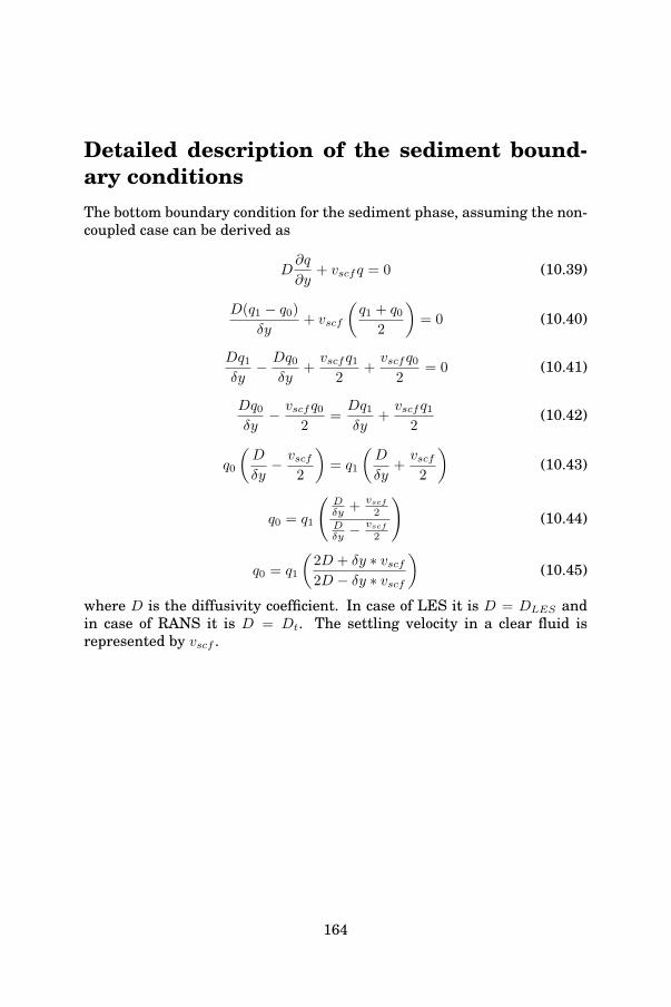
Detailed description of the sediment bound-ary conditionsThe bottom boundary condition for the sediment phase, assuming the non-coupled case can be derived as
D∂q
∂y+ vscfq = 0 (10.39)
D(q1 − q0)
δy+ vscf
(q1 + q0
2
)= 0 (10.40)
Dq1
δy− Dq0
δy+vscfq1
2+vscfq0
2= 0 (10.41)
Dq0
δy− vscfq0
2=Dq1
δy+vscfq1
2(10.42)
q0
(D
δy− vscf
2
)= q1
(D
δy+vscf
2
)(10.43)
q0 = q1
(Dδy +
vscf2
Dδy −
vscf2
)(10.44)
q0 = q1
(2D + δy ∗ vscf2D − δy ∗ vscf
)(10.45)
where D is the diffusivity coefficient. In case of LES it is D = DLES andin case of RANS it is D = Dt. The settling velocity in a clear fluid isrepresented by vscf .
164

Top boundary condition for the sediment phase, assuming the non-coupledcase can be derived as
D∂q
∂y+ vscfq = 0 (10.46)
D(qN − qN−1)
δy+ vscf
(qN + qN−1
2
)= 0 (10.47)
DqNδy− DqN−1
δy+vscfqN
2+vscfqN−1
2= 0 (10.48)
DqNδy
+vscfqN
2=DqN−1
δy− vscfqN−1
2(10.49)
qN
(D
δy+vscf
2
)= qN−1
(D
δy− vscf
2
)(10.50)
qN = qN−1
(Dδy −
vscf2
Dδy +
vscf2
)(10.51)
qN = qN−1
(2D − δy ∗ vscf2D + δy ∗ vscf
)(10.52)
where D is the diffusivity coefficient. In case of LES it is D = DLES andin case of RANS it is D = Dt. The settling velocity in a clear fluid isrepresented by vscf .
165

166

List of Publications
Journal articles1. Widera, P., Toorman, E. and Lacor, C., Large eddy simulation of sed-
iment transport in open-channel flow. Journal of Hydraulic Research,47(3), pp. 291-298, 2009
2. Widera, P., Ghorbaniasl, G. and Lacor, C., Study of the sedimenttransport over flat and wavy bottom using large-eddy simulation.Journal of Turbulence, 10(33), pp. 1 - 20, 2009
3. Ghorbaniasl, G., Widera, P. and Lacor C., Quality of dynamic vari-ational multiscale models on distorted grids. Journal of Turbulence,10(22), pp. 1 - 19, 2009
4. Widera, P. and Lacor C., Study on slip velocity models and theirapplicability to sedimentation problems. Journal of Hydraulic Re-search, Submitted for publication.
5. Widera, P. and Lacor C., Study on interaction between sediment andfluid using large-eddy simulation. Journal of Turbulence, Submittedfor publication.
6. Ghorbaniasl, G., Widera, P. and Lacor C., On the estimation of subgrid-scale model coefficients. Journal of Turbulence, Submitted for publi-cation.
Conference proceedings1. Widera, P., Toorman, E. and Lacor, C., Large eddy simulation of sed-
iment transport in open-channel flow. Ercoftac Belgian Pilot CenterAnnual Seminar. UCL, Louvain-le-Neuve, Dec 8, 2006 .
167

2. Awad, E., Toorman, E., Widera, P. and Lacor, C., Large Eddy Sim-ulations for quasi-2D turbulence in shallow flows, Turbulence Revis-ited (Abstracts ILCOD2008 and Warnemunde Turbulence Days). Int.Liege Colloquium on Ocean Dynamics and Warnemunde TurbulenceDays. Liege (Belgium), May 2007.
3. Toorman, E., Lacor, C., Awad, E., Heredia, M. and Widera, P., Scaleproblems in 3D sediment transport models and suggestions to over-come them. In : Qualite des Eaux Marines Colloque SHF PollutionMaritime. Paris (France) (pp. 1-8), Socit Hydraulique de France, 22-23 January, 2007
4. Toorman, E., Lacor, C., Heredia, M. and Widera, P., Upscaling near-bottom sediment-turbulence interaction effects for large-scale 3D sed-iment transport modelling, Turbulence Revisited (Abstracts Int. LiegeColloquim on Ocean Dynamics and Warnemunde Turbulence Days).Int. Liege Colloqium on Ocean Dynamics and Warnemunde Turbu-lence Days. Liege (Belgium), May 2007.
5. Toorman, E., Heredia, M., Lacor, C. and Widera P., A three-layer tur-bulence model for the study of near-bed sediment transport, Book ofAbstracts INTERCOH’07. Int. Conf. on Coastal and Estuarine Cohe-sive Sediment Transport, (69), Brest (France): IFREMER, September2007
6. Ghorbaniasl, G., Widera, P., Hirsch, C. and Lacor, C., A numeri-cal simulation of sound wave from permeable surfaces, Edition: Pro-ceedings of Mathematical modeling of wave phenomena, publishedby: Mathematical modeling of wave phenomena, Sweden, 2008
7. Toorman, E., Widera, P., Heredia, M. and Lacor, C., Upscaling ofbottom-generated turbulence in large-scale 3D models for sedimenttransport in estuaries and coastal zones, Proc. EGU2008. EGU 2008.Vienna, May 2008 EGU, 2008
8. Ghorbaniasl G., Widera, P., Van Den Abeele, K. and Lacor, C., ADynamic Variational Multiscale Model in Turbulent Channel Flowwith Distorted Grids, Edition:47th AIAA Aerospace Sciences Meetingand Exhibit, 5-8 January 2009, Orlando, Florida (paper), 2009
9. Widera, P., and Lacor, C., Investigation on the influence of varioussediment-fluid coupling approaches to the flow and sediment trans-port, National Conference on Theoretical and Applied Mechanics, Brus-sels, Belgium), 28-29 May, 2009
168

10. Widera P., and Lacor, C., Study on slip velocity models and their ap-plicability to sedimentation problems, Ercoftac Belgian Pilot CenterAnnual Seminar. CENAERO, Gosselies, Dec 10, 2010 .
169

170

Bibliography
[1] AHRENS, J. A fall-velocity equation. Journal of Waterway, Port,Coastal and Ocean Engineering 126, 2 (2000), 99–102.
[2] ALLEN, J. Principles of physical sedimentology., first edition ed. G.Allen & Unwin in London, Boston, 1985.
[3] ARRHENIUS, S. The viscosity of solutions. Biochemical Journal 11,2 (1917), 112–133.
[4] ASHRAFIAN, A., ANDERSSON, H., AND MANHART, M. DNS of tur-bulent flow in a rod-roughened channel. International Journal ofHeat and Fluid Flow 25 (2004), 373–383.
[5] BAGHI, P., AND BALACHANDAR, S. Effect of turbulence on the dragand lift of particle. Physics of Fluids 15 (2003), 3496–3513.
[6] BARNES, H. A., HUTTON, J. F., AND WALTERS, K. An introduc-tion to rheology. Elsevier Science Publishers B. V., Amsterdam, TheNetherlands (1989).
[7] BATCHELOR, G. The effect of brownian motion on the bulk stress ina suspension of spherical particles. Journal of Fluid Mechanics 83(1977), 97–117.
[8] BESNARD, D. C., BURESI, E., HERMELINE, F., AND WAGON, F. Nondeterministic methods for charged particle transport. Monte-CarloMethods and Applications in Neutronics, Photonics, and StatisticalPhysics. Proceedings of the Joint Los Alamos National Laboratory-Commissariat l’Energie Atomique Meeting, held at Cadarache Cas-tle, Provence, France, April 22-26 Lecture Notes in Physics, Vol. 240,edited by R. Alcouffe, R. Dautray, A. Forster, G. Ledonois, and B.Mercier. Springer-Verlag, Berlin, (1985), 126p.
171

[9] BHAGANAGAR, K., KIM, J., AND COLEMAN, G. Effects of roughnesson wall-bounded turbuence. International Journal of Heat and FluidFlow 72 (2004), 463–492.
[10] BOERSMA, B. Particle distributions in the flow over a wavy wall.In Studying Turbulence Using Numerical Simulation Databases -VIII (Center for Turbulence Research, Building 500, Room 500A,488 Escondido Mall, Stanford University, Stanford, CA 94305-3035,November 2000), M. P., R. W.C., and M. N.N., Eds., Stanford Univer-sity, p. pp. 352.
[11] BOERSMA, W., LAVEN, J., AND STEIN, H. Computer simulations ofshear thickening of concentrated dispersions. Journal of Rheology39 (1995), 841–859.
[12] BOSSE, T., KLEISER, L., AND MEIBURG, E. Small particles in ho-moenous turbulence: Settling velocity enhancement by two-way cou-pling. Physics of Fluids 18 (2006).
[13] BOUDERAU, B. Geomorphological factors influencing the formationof shore-normal sediment streaks in the swash zone.
[14] BRADY, J. The rheological behavior of colloidal dispersions. Journalof Chemical Physics 99 (1993), 567–581.
[15] BREDBERG, J. On two-equation eddy-viscosity models. Tech. rep.,2001.
[16] BREDBERG, J. Turbulence Modelling for Internal Cooling of Gas-Turbine Blades. PhD thesis, Dept. of Thermo and Fluid Dynamics,Chalmers University of Technology, Goteborg, Sweden, 2002.
[17] BURBAN, P., XU, Y., MCNEIL, J., AND LICK, W. Settling speeds offlocs in fresh water and seawater. Journal of Geophysical Research95, C10 (1990), 18,213–18,220.
[18] CABOT, W., AND MOIN, P. Large Eddy Simulation of scalar trans-port with the dynamic subgrid-scale model. Cambridge UniversityPress, 1993.
[19] CAMENEN, B. Simple and general formula for the settling velocityof particles. Journal of Hydraulic Engineering 133 (2007), 229–233.
[20] CANCINO, L., AND NEVES, R. Hydrodynamic and sediment suspen-sion modelling in estuarine systems. part i:description of the numer-ical models. Journal of Marine Systems 22 (1999), 105–116.
172

[21] CELLINO, M. Experimental study of suspension flow in open chan-nels. PhD thesis, Ecole Polytechnique Federale de Lausanne, Lau-sanne, Switzerland, 1998.
[22] CELLINO, M., AND GRAF, W. Sediment-laden flow in open channelsunder noncapacity and capacity conditions. Journal of HydraulicEngineering 125 (1999).
[23] CHANSON, H. Extreme reservoir siltation in australia: A review.International Journal of Sediment Research 13, 3 (1998), 55–63.
[24] CHENG, N. Simplified settling velocity formula for sediment parti-cle. Journal of Hydraulic Engineering 123, 2 (1997), 149–152.
[25] CHENG, N., AND LAW, A. Exponential formula for computing effec-tive viscosity. Powder Technology 129, 1-3 (2003), 156–160.
[26] CHERUKAT, P., NA, Y., HANRATTY, T., AND MCLUGHLIN, J. Di-rect numerical simulation of a fully developed trubulent flow overa wavy wall. Theoretical and Computational Fluid Dynamics 11(1998), 109–134.
[27] CHIEN, K. Predictions of channel and boundary-layer flows with alow-reynolds number turbulence model. AIAA Journal 20, 1 (1982),33–38.
[28] CHOI, H. S., AND SUZUKI, K. Large eddy simulation of turbulentflow and heat transfer in a channel with one wavy wall. Interna-tional Journal of Heat and Fluid Flow (2005).
[29] CHONG, J., CHRISTIANSEN, E., AND BAER, A. Rheology of concen-trated suspensions. Journal of Applied Polymer Science 15 (1971),2007–2021.
[30] COOPERA, D., AND CLOUGHA, D. Experimental tracking of particle-size distribution in a fluidized bed. Powder Technology 44 (1985),169–177.
[31] COURANT, R., FRIEDRICHS, K., AND LEWY, H. On the partial dif-ference equations of mathematical physic. IBM Journal March 1967(1967), 215–234.
[32] COUSSOT, P. Mudflow rheology and dynamics. IAHR mono-graph series (International Association for Hydraulic Research), A.A.Balkema, Rotterdam, Netherlands (1997), 255 p.
173

[33] DAVIDSON, L. An introduction to turbulence models. Tech. rep.,2003.
[34] DE BRYE, B., DE BRAUWERE, A., GOURGUE, O., KARNA, T., LAM-BRECHTS, J., COMBLEN, R., AND DELEERSNIJDER, E. A finite-element, multi scale model of the scheldt tributaries, river, estuaryand rofi. Coastal Engineering 57 (2010), 850–863.
[35] DYTER, K. The initiation of sedimentary turrows by standing inter-nal waves. Sedimentology 29 (1982), 885–889.
[36] EINSTEIN, A. Effect of suspended rigid spheres on viscosity. Annu-als of Physics 19 (1906), 289–306.
[37] EINSTEIN, H. A., AND BARBAROSSA, N. River channel roughness.Journal of Hydraulic Engineering 117 (1952).
[38] ELGHOBASHI, S. On predicting particle-laden turbulent flows. Ap-plied Scientific Research 52 (1994), 309–329.
[39] ENGELUND, F., AND HANSEN, E. A monograph on sediment trans-port in alluvial streams. Technisk Vorlag, Copenhagen, Denmark(1967).
[40] FAN, L., AND ZHU, C. Principles of gas-solid flows. CambridgeUniversity Press, 1998.
[41] FAVRE, A. Equations statistiques aux fluctuations turbulentesd’entropie, de concentration, de rotationnel, dans les coulementscompressibles. C. R. Acad. Sci. Paris Ser. 273 (1971), A1289–A1294.
[42] GERMANO, M., PIOMELLI, U., MOIN, P., AND CABOT, W. A dynamicsubgrid-scale eddy viscosity model. Physics of Fluids A 3 (1991),1760.
[43] GERMANO, M., PIOMELLI, U., MOIN, P., AND CABOT, W. A dynamicsubgrid-scale eddy viscosity model. Physics of Fluids A3(7) (1991).
[44] GHORBANIASL, G. Overview of subgrid scale models. Internal re-port, Vrije Universiteit Brussel, November 2006.
[45] GHORBANIASL, G. Computational aeroacoustic-noise prediction us-ing hybrid methodologies. Phd thesis, Vrije Universiteit Brussel,2009.
[46] GHORBANIASL, G., AND LACOR, C. Sensitivity of sgs models and ofquality of les to grid irregularity. In Quality and Reliability of Large-Eddy Simulations (2008), M. J., G. B., and S. P., Eds., Springer.
174

[47] GIBBS, R. Estuarine flocs: their size, settling velocity and density.Journal of Geophysical Research 28, C2 (1985), 3,249–3,251.
[48] GIBBS, R. J., MATHEWS, M. D., AND LINK, D. A. Settling velocityof natural particles. J. Sediment. Petrol. 44, 1 (1971), 7–18.
[49] GILBERT, R., ZEDLER, E., GRILLI, T., AND STREET, R. Modellingof wave driven sediment transport over a partially buried cylinder.Ocean Waves Measurement and Analysis Fifth Interantional Sympo-sium WAVES 2005 (2005).
[50] GRAF, W., AND CELLINO, M. Suspension flows in open channels: ex-perimental study. IAHR Journal of Hydraulic Research 40, 4 (2002),435–447.
[51] GRASS, J. Structural features of turbulent flow over smooth andrough boundaries. Journal of Fluid Mechanics 50 (1971), 233–255.
[52] GREIMANN, B., MUSTE, M., AND HOLLY, F. J. Two-phase formu-lation of suspended sediment transport. Journal of Hydraulic Re-search 37, 4 (2000), 479–500.
[53] HAIDER, A., AND LAVENSPIEL, O. Drag coefficient and terminalvelocity of spherical and non-spherical particles. Powder Technology58 (1989), 63–70.
[54] HAPPEL, J. Viscosity of suspensions of uniform spheres. Journal ofApplied Physics 28 (1957), 12881292.
[55] HEREDIA, M. Numerical modelling of turbulent flow over rough sur-faces. PhD thesis, Dept. of Burgerlijke Bouwkunde Laboratoriumvoor Hydraulica, Katholieke Universiteit Leuven, Leuven, Belgium,2009.
[56] HIBIKI, T., AND ISHII, M. One-dimensional drift-flux model andconsitutive equations for relative motion between phases in varioustwo-phase flow regimes. International Journal of Heat and MassTransfer 46 (2003), 4935–4948.
[57] HIRSCH, C. Numerical Computation of Internal and External Flows,Volume 1: Fundamentals of Numerical Discretisation. John Wiley &Sons, 1988.
[58] HIRSCH, C. Numerical Computation of Internal and External Flows,Volume 2: Computatinal Methods for Inviscid and Viscous Flows.John Wiley & Sons, 1990.
175

[59] HIRSCH, C. Numerical Computation of Internal and External Flows.Butterworth-Heinemann, 2007.
[60] HRENYA, C., BOLIO, E., CHAKRABARTI, D., AND SINCLAIR, J.Comparison of low Reynolds number k− ε turbulence models in pre-dicting fully developed pipe flow. Chemical Engineering Science 50(1995), 1923–1941.
[61] HUDSON, J., DYKHNO, L., AND HANRATTY, T. Turbulence produc-tion in flow over a wavy wall. Experiments in Fluids 20 (1996), 256–265.
[62] HWANG, K.-N. Erodibility of fine sediment in wave dominated en-vironments. MS Thesis Gainesville FL, US (University of Florida),166.
[63] ILIC, V., AND PHAN-TIEN, N. Viscosity of concentrated suspensionsof spheres. Rheologica Acta 33 (1994), 283–291.
[64] ISHII, M., AND MISHIMA, K. Two-fluid model and hydrodynamicconstitutive relations. Nuclear Engineering and Design 82 (1984),107–126.
[65] JAMESON, A., SCHMIDT, W., AND TURKEL, E. Numerical simula-tion of euler equations by finite volume methods using runge-kuttatime stepping schemes. AIAA Journal 81-1259 (1981).
[66] JIANG, J., LAW, A., AND CHENG, N. Two-phase modeling of sus-pended sediment distribution in open channel flows. Journal of Hy-draulic Research 42, 3 (2004), 273–281.
[67] JIMENEZ, J. Turbulent flows over rough walls. Annual Review ofFluid Mechanics 36 (2004), 173–196.
[68] JIMENEZ, J., AND MADSEN, O. A simple formula to estimatesettling velocity of natural sediments. Journal of Waterway, Port,Coastal and Ocean Engineering 129, 2 (2003), 70–78.
[69] KAFTORI, D., HETSRONI, G., AND BANERJEE, S. Particle behaviorin the turbulent boundary layer. i. motion, deposition, and entrain-ment. Physics of Fluids 7, 5 (1995), 1095–1106.
[70] KAFTORI, D., HETSRONI, G., AND BANERJEE, S. Particle behaviorin the turbulent boundary layer. ii. velocity and distribution profiles.Physics of Fluids 7, 5 (1995), 1106–121.
176

[71] KEYLOCK, C., HARDY, R., PARSONS, D., FERGUSON, R., LANE,S., AND RICHARDS, K. The theoretical foundations and potentialfor LES in fluvial geomorphic and sedimentological research. EarthScience Reviews 71 (2005).
[72] KRIEGER, I., AND DOUGHERTY, T. Concentration dependence of theviscosity of suspensions. Trans. Soc. Rheol. 3 (1959), 137–152.
[73] KRISHNAPPAN, B., AND MARSALEK, J. Modelling of flocculationand transport of cohesive sediment from an on-stream stormwaterdetention pond. Water Research 36 (2002), 3849–3859.
[74] KUZAN, J., ADRIAN, R., AND HANRATTY, T. Turbulence flowswith incipient separation over solid waves. Experiments in Fluids7 (1989), 88–98.
[75] LACOR, C. Lecture notes. Dept. Fluid Mechanics, Vrije UniversiteitBrussel, Brussels, Belgium, 2007.
[76] LAUWAERT, B., BEKAERT, K., BERTELOOT, M., DE BACKER, A.,DERWEDUWEN, J.AND DUJARDIN, A., FETTEWIS, M., HILLEW-ERT, H., HOFFMAN, S., HOSTENS, K., IDES, S., J., J., MARTENS,C., MICHIELSEN, T., PARMENTIER, K., VAN HOEY, G., AND VER-WAEST, T. Synthesis report on the effects of dredged material dis-posal on the marine environment (licensing period 2008-2009). Re-port by MUMM, ILVO Fisheries, Maritime Access Division (aMT),and Coast Division (CD), Belgium Report Number BL/2009/01(2009), pp. 109.
[77] LEE, C. Large eddy simulation of rough-wall turbulent bound-ary layers. American Institute of Aeronautics and Astronautics 40(2002), 2127–2130.
[78] LEE, D. The viscosity of concentrated suspensions. Transactions ofthe Society of Rheology 13, 2 (1969), 273–288.
[79] LELY, M. Hydraulic roughness in sediment-laden flow.
[80] LEONARDI, S., ORLANDI, P., SMALLEY, R., DJENIDI, L., AND AN-TONIA, R. Direct numerical simulations of turbulent flow withtransverse square bars on one wall. Journal of Fluid Mechanics 491(2003), 229–238.
[81] LILLY, D. A proposed modification of the Germano subgrid-scalemodel. Physics of Fluids A 4(3) (1992).
177

[82] LONGEST, P., AND OLDHAM, M. Numerical and experimental depo-sition of fine respiratory aerosols: Development of a two-phase driftflux model with near-wall velocity corrections. Journal of AerosolScience 39 (2008), 48–70.
[83] MA, G., SHI, F., LIU, S., AND QI, D. Hydrodynamic modeling ofchangjiang estuary: Model skill assessment and large-scale struc-ture impacts. Applied Ocean Research 33 (2011), 69–78.
[84] MANNINEN, M., TAIVASSALO, V., AND KALLIO, S. On the mix-ture model for multiphase equation. Tech. rep., Valtion TeknillinenTutkimuskeskus, Espoo, Finland, 1996.
[85] MARCHIOLI, C., PICCIOTTO, M., AND SOLDATI, A. Influence ofgravity and lift on particle velocity statistics and transfer rates inturbulent vertical channel flow. International Journal of MultiphaseFlow 33 (2007), 227–251.
[86] MATHIS, M., KERBYSON, D., AND A., H. A performance model ofnon-deterministic particle transport on large scale systems. Interna-tion Conference on Computational Science,Saint Petersburg, RussianFederation, Melbourne, Australia LNCS 2659 (2003), 905–915.
[87] MAXEY, M. R. The gravitational settling of aerosol particles in ho-mogeneous turbulence and random flow fields. Journal of Fluid Me-chanics 174 (1987), 441–465.
[88] MAXIMOVA, T., IDES, S., DE MULDER, T., AND MOSTAERT, F. Ver-betering randvoorwaardenmodel. deelrapport 4: Extra aanpassin-gen in de zeeschelde. Report by Waterbouwkundig Laboratorium,Flanders Hydraulics Research, Antwerp, Belgium WL Rapporten,WL2009R753/09/4rev2/0 (December 2009), pp. 104.
[89] MAZUMDER, R. Turbulenceparticle interactions and their implica-tions for sediment transport and bedform mechanics under unidirec-tional current: some recent developments. Earth-Science Reviews 50(2000), 113–124.
[90] MEHTA, A. Laboratory studies on cohesive sediment deposition anderosion. In: Dronkers J. and van Leussen W. (Eds.) Physical processesin estuaries (1988), 427–445.
[91] MEHTA, A., AND PARTHENIADES, E. An investigation of the deposi-tional properties of flocculated fine sediments. Journal of HydraulicResearch 13 (1975), 361–381.
178

[92] MEHTA, A.J. AND LI, Y. A PC based short course on fine-grainedsediment transport engineering. Coastal and Oceanographic Engi-neering Department, University of Florida, USA, 1995.
[93] MIYAKE, Y., TSUJIMOTO, K., AND NAGAI, N. Numerical simulationof channel flow with a rib-roughened wall. Journal of Turbulence 035(2002).
[94] MOONEY, J. The viscosity of a concentrated suspension of sphericalparticles. Journal of Colloid Science 6 (1951), 162–170.
[95] MORSI, S., AND ALEXANDER, A. An investigation of particle tra-jectories in two-phase flow systems. Journal of Fluid Mechanics 55(1972), 193–208.
[96] MOSER, R. D., KIM, J., AND MANSOUR, N. N. Direct numericalsimulation of turbulent channel flow up to Re tau=590. Physics ofFluids 11 (1999).
[97] MURRAY, S. P. Settling velocities and vertical diffusion of parti-cles in turbulent water. Journal of Sedimentary Petrology 75 (1970),1647–1654.
[98] NAKAGAWA, S., AND HANRATTY, T. Influence of a wavy boundaryon turbulence. ii. intermediate roughened and hydraulically smoothsurface. Experiments in Fluids 35 (2003), 437–447.
[99] NAKAGAWA, S., NA, Y., AND HANRATTY, T. Influence of a wavyboundary on turbulence. i. highly rough surface. Experiments in Flu-ids 35 (2003), 422–436.
[100] NICHOLSON, J., AND O’CONNOR, B. Cohesive sediment transportmodel. Journal of Hydraulic Engineering 111 (1986), 621–640.
[101] NICOUD, F., AND DUCROS, F. Subgrid-scale stress modeling basedon the square of the velocity gradient tensor. Flow, Turbulence Com-bust. 62 (1999), 182–200.
[102] NIELSEN, P. Turbulence effects on the settling of suspended parti-cles. Journal of Sedimentary Petrology 63 (1993), 835–838.
[103] NIKURADSE, J. Laws of flow in rough pipes. Technical Memoran-dum NACA-TM-1292, NASA, 1950.
[104] ORLANDI, P., LEONARD, S., TUZI, R., AND ANTONIA, R. Directnumerical simulation of turbulent channel flow with wall velocitydisturbances. Physics of Fluids 15, 12 (2003).
179

[105] ORLANDI, P., AND LEONARDI, S. Passive scalar in a turbulent chan-nel flow with wall velocity disturbances. Flow, Turbulence and Com-bustion 72 (2004), 181–197.
[106] ORLANDI, P., LEONARDI, S., DJENIDI, L., AND ANTONIA, R. Struc-ture of turbulent channel flow with square bars on one wall. Inter-national Journal of Heat and Fluid Flow 25 (2004), 384–392.
[107] PAN, Y., TANAKA, T., AND TSUJI, Y. Direct numerical simulationof particle-laden rotating turbulent channel flow. Physics of FLuids13, 8 (2001), 2320–2337.
[108] PICCIOTTO, M., MARCHIOLI, C., REEKS, M. W., AND SOLDATI,A. Statistics of velocity and preferential accumulation of micro-particles in boundary layer turbulence. Nuclear Engineering andDesign 235 (2005), 1239–1249.
[109] PIOMELLI, U. Application of large eddy simulations in engineering:an overview. In Large eddy simulation of complex engineering andgeophysical flows (1993), G. B. and O. S., Eds., Cambridge UniversityPress.
[110] PIOMELLI, U., AND BENOCCI, C., V. B. J. Large eddy simulationand related techniques, theory and applications. Tech. rep., von Kar-man Institute for Fluid Dynamics, 13-16,March 2006.
[111] PIOMELLI, U., MOIN, P., AND FERZIGER, J. Model consistency inlarge eddy simulation of turbulent channel flows. Physics of Fluids31, 7 (1984), 1884–1891.
[112] POLETTO, M., AND JOSEPH, D. Effective density and viscosity of asuspension. The Society of Rheology 39 (1994).
[113] POPE, S. B. Turbulent flows. Cambridge university press, New York,2000.
[114] RICHARDSON, J., AND ZAKI, W. Sedimentation and fluidization.Transactions of the Institute of Chemical Engineering 32 (1954), 35–53.
[115] ROSCOE, R. The viscosity of suspensions of rigid spheres. BritishJournal of Applied Physics 3, 8 (1952), 267.
[116] RUTGERS, J. Relative viscosity of suspensions of rigid spheres innewtonian liqiud. Reologica Acta 2 (1962), 202–212.
180

[117] SCHIEBER, J., SOUTHARD, J., AND SCHIMMELMANN, A. Lenticularshale fabrics resulting from intermittent erosion of water-rich muds-interpreting the rock record in the light of recent flume experiment.Journal of Sedimentary Research 80 (2010), 119–128.
[118] SCHIEBER, J., SOUTHARD, J., AND THAISEN, K. Accretion of mud-stone beds from migrating floccule ripples. Science 318 (2007), 1760–1762.
[119] SCHILLER, L., AND NAUMANN, A. Uber die grundlagenden berech-nungen bei der schwerkraftaufbereitung. Ver. Deut. Ing. Z. 77 (1933),318–320.
[120] SCHLICHTING, H. Experimentelle untersuchungen zum rauhigkeit-sproblem. Archive of Applied Mechanics (Ingenieur Archiv) 7, 1(1936), 1–34.
[121] SCHRAIBER, A., GAVIN, L., NAUMOV, V., AND YATSENKO, V. Tur-bulent flows in gas suspensions. Hemisphere Publishing CorporationNew York (1990).
[122] SMAGORINSKY, J. General circulation experiments with the primi-tive equation. Monthly Weather Report 91-3 (1963), 99–106.
[123] STOESSER, T., MATHEY, F., FROHLICH, J., AND RODI, W. LES offlow over multiple cubes. ERCOFTAC Bulletin MARCH (2003).
[124] STOLL, R., AND PORTE-AGEL, F. Dynamic subgrid-scale modelsfor momentum and scalar fluxes in LES of neutrally stratified atmo-spheric boundary layers over heterogenous terrain. Water ResourcesResearch (2005).
[125] STRUBLE, L., AND SUN, G. Viscosity of portland cement past asa function of temperature. Advanced Cement Based Materials 2(1995), 62–69.
[126] SWAMEE, P., AND OJHA, C. Closure of discussion on drag coefficientand fall velocity of nonspherical particles. Journal of Hydraulic En-gineering 117, 11 (1991), 15911592.
[127] SWAMEE, P., AND OJHA, C. Drag coefficient and fall velocity of non-spherical particles. Journal of Hydraulic Engineering 117, 5 (1991),660–667.
[128] TAYLOR, J. R., SARKAR, S., AND ARMENIO, V. Large eddy simu-lation of stably stratified open channel flow. Physics of Fluids 17(2005).
181

[129] THOMAS, C., AND MUTHUKUMAR, M. Three-body hydrodynamiceffect on viscosity of suspensions of spheres. Journal of ChemicalPhysics 94, 7 (1991), 5180–5189.
[130] THOMAS, D. Transport characteristics of suspension: Viii. a noteon the viscosity of newtonian suspensions of uniform spherical par-ticles. Journal of Colloid Science 20 (1965), 267–277.
[131] TODA, K., AND HISAMOTO, F. Extension of einstein’s viscosity equa-tion to that for concentrated dispersions of solutes and particles.Journal of Bioscience and Bioengineering 102, 6 (2006), 524–528.
[132] TOFALETTI, F. A procedure for computation of total river sand dis-charge and detailed distribution, bed to surface. Committee on Chan-nel Stabilisation, U.S. Army Corps of Engineers Report No. 5 (1968).
[133] TOOBY, P., WICK, G., AND ISAACS, J. The motion of a small spherein a rotating velocity field: A possible mechanism for suspendingparticles in turbulence. Journal of Geophysical Research 82 (1977),2096–2100.
[134] TOORMAN, E. Analysis of near-wall turbulence modelling withk − ε model. Tech. Rep. HYD/ET/00/COSINUS2, Katholieke Uni-versiteit Leuven, Hydraulics Laboratory, Civil Engineering Depart-ment, Katholieke Universiteit Leuven, Kasteelpark Arenberg 40, B-3001 Heverlee (Leuven), Belgium, December 2000.
[135] TOORMAN, E. Drag reduction in sediment-laden turbulentflows. Tech. Rep. HYD/ET/00/COSINUS/5, Katholieke UniversiteitLeuven, Hydraulics Laboratory, Civil Engineering Department,Katholieke Universiteit Leuven, Kasteelpark Arenberg 40, B-3001Heverlee (Leuven), Belgium, December 2000.
[136] TOORMAN, E. Parameterization of turbulence damping in sediment-laden flow. Tech. Rep. HYD/ET/00/COSINUS/3, Katholieke Uni-versiteit Leuven, Hydraulics Laboratory, Civil Engineering Depart-ment, Katholieke Universiteit Leuven, Kasteelpark Arenberg 40, B-3001 Heverlee (Leuven), Belgium, December 2000.
[137] TOORMAN, E. Sediment-laden turbulent flow: A review of theoriesand models. Tech. Rep. HYD/ET/00/COSINUS1, Katholieke Uni-versiteit Leuven, Hydraulics Laboratory, Civil Engineering Depart-ment, Katholieke Universiteit Leuven, Kasteelpark Arenberg 40, B-3001 Heverlee (Leuven), Belgium, December 2000.
182

[138] TOORMAN, E. Some thoughts on the modelling of erosion and de-position of cohesive sediments. Tech. Rep. HYD/ET/00/COSINUS/7,Katholieke Universiteit Leuven, Hydraulics Laboratory, Civil Engi-neering Department, Katholieke Universiteit Leuven, KasteelparkArenberg 40, B-3001 Heverlee (Leuven), Belgium, December 2000.
[139] TOORMAN, E. Suspension capacity of uniform shear flows. Tech.Rep. HYD/ET/00/COSINUS/4, Katholieke Universiteit Leuven, Hy-draulics Laboratory, Civil Engineering Department, Katholieke Uni-versiteit Leuven, Kasteelpark Arenberg 40, B-3001 Heverlee (Leu-ven), Belgium, December 2000.
[140] TOORMAN, E. Validation of macroscopic modelling of particle-ladenturbulent flows. In Proceedings 6th Belgian National Congress onTheoretical and Applied Mechanic (2003).
[141] TOORMAN, E. Vertical flux and momentum balance in sediment-laden turbulent open-channel flow at equilibrium. Journal of Hy-draulic Engineering accepted for publication (2007).
[142] TOORMAN, E. Vertical mixing in the fully developed turbulent layerof sediment-laden open channel flow. Journal of Hydraulic Engineer-ing 134, 9 (2008), 1225–1235.
[143] TOORMAN, E. Errata and addendum for ”vertical mixing in the fullydeveloped turbulent layer of sediment-laden open channel flow” bye.a. toorman. Journal of Hydraulic Engineering 135, 6 (2009), 538.
[144] TSENG, Y.-H., AND FERZIGER, J. Large eddy simulation of turbu-lent wavy boundary flow - illustration of vortex dynamics. Journalof Turbulence (2004).
[145] VAN KESSEL, T., VANLEDE, J., AND DE KOK, J. Development ofa mud transport model for the scheldt estuary. continental ShelfResearch doi:10.1016/j.csr.2010.12.006 (2011), pp. 17.
[146] VAN RIJN, L. Computation of bed load and suspended load. ReportS487-II (1982).
[147] VAN RIJN, L. Sediment transport, part ii: suspended load transport.Journal of Hydraulic Engineering 110, 11 (1984), 1431–1456.
[148] VAN RIJN, L. Sediment transport, parti : bed load transport. Jour-nal of Hydraulic Engineering 110, 10 (1984), 1431–1456.
[149] VAN RIJN, L. Principles of sediment transport in rivers, estuariesand coastal seas. Aqua Publications (1993).
183

[150] VAND, V. Theory of viscosity of concentrated suspensions. Nature155 (1945), 364–365.
[151] VILLARET, C., AND DAVIES, A. Modeling sediment-turbulent flowinteractions. Applied Machanical Review 49, 9 (1995), 601–609.
[152] WIDERA, P., GHORBANIASL, G., AND LACOR, C. Study of the sedi-ment transport over flat and wavy bottom using large-eddy simula-tion. Journal of Turbulence 10, 33 (2009), 1–20.
[153] WIDERA, P., TOORMAN, E., AND LACOR, C. Large eddy simulationof sediment transport in open-channel flow. Journal of HydraulicResearch 47, 3 (2009), 291–298.
[154] WILCOX, D. Turbulence modeling for CFD. DCW Industries, Inc,California, 1998.
[155] WINCKELMANS, G., JEANMART, H., AND CARATI, D. On the com-parison of turbulence intensities from large-eddy simulation withthose from experiment or direct numerical simulation. Physics ofFluids 14, 5 (2002), 1809–1811.
[156] WINTERWERP, J., AND VAN KESTEREN, W. Introduction to thePhysics of Cohesive Sediment in the Marine Environment., first edi-tion ed. No. 56 in Developments in Sedimentology Series. Amster-dam: Elsevier, 2004.
[157] WREN, D., BENNETT, S., BARKDOLL, B., AND KUHNLE, R. Studiesin suspended sediment and turbulence in open channel flow. Re-search Report No. 18 (2000).
[158] WU, W. Computational River Dynamics. Taylor & Francis, 2008.
[159] YAMAMOTO, Y., POTTHOFF, M., TANAKA, T., KAJISHIMA, T., ANDTSUJI, Y. Large eddy simulation of turbulent gas-particle flow in avertical channel: effect of considering inter-particle collisions. Jur-nal of Fluid Mechanics 442 (2001), 303–334.
[160] YANG, C., AND SIMOES, F. Generalized sediment transport modelfor alluvial river simulation. U.S. Bureau of Reclamation, TechnicalSErvice Center, Colorado ver. 3.0 (2002).
[161] YOON, J., AND KANG, S. A numerical model of sediment-laden tur-bulent flow in an open channel. Canadian Journal of Civil Engineer-ing 32 (2005), 233–240.
184

[162] ZANKE, U. Berechung der sinkgeschwindigkeiten von sedimenten.Mitt. Des Franzius-Instituts fuer Wasserbau, Technische Universi-taet, Hannover,Deutschland 46, page 243 (1977).
[163] ZEDLER, E., AND STREET, R. Large-Eddy simulation of sedimenttransoprt: currents over ripples. Journal of Hydraulic Engineering127, 6 (2001), 444–452.
185


The main objective of research described in this thesis is a study of the sed-iment transport in fluids using Large Eddy Simulation (LES) and ReynoldsAveraged Navier Stokes (RANS) methodologies, with the emphasis on thedevelopment of the LES methodology. Thesis consists of the code descrip-tion, its development and investigation of the sediment transport pro-cesses in fluids. The specific objectives of this study were outlined as fol-lows.
1. Applicability of LES methodology to the sediment transport processes
2. Example of improvement of the RANS models based on the LES re-sults
3. Investigation on the turbulent Schmidt number profile in case ofchannel with a smooth and rough bottom
4. Investigation on the fluid-sediment coupling
5. Investigation on the slip velocity models for the sediment
Results obtained from simulations were as expected. It has been provedby comparing with theoretical model that the LES methodology is use-ful and gives very accurate results of sediment concentration. The LESapproach gives also the possibility to investigate such a phenomenon as aturbophoresis or the sediment uplifting in the bottom region. It was provedthat the large eddy simulation technique has a big potential in further in-vestigations of the sediment transport as well as in the improvement ofRANS methodology in order to get more accurate results for a real life andlarge scale test cases.