materials

Article

Study of Flexural Response in Strain HardeningCementitious Composites Based on ProposedParametric Model

Zhanfeng Qi , Zhiyi Huang *, Hui Li and Wenhua Chen

College of Civil Engineering and Architecture, Zhejiang University, Hangzhou 310000, China;qizhanfeng@zju.edu.cn (Z.Q); 21612089@zju.edu.cn (H.L.); 11812061@zju.edu.cn (W.C.)* Correspondence: hzy@zju.edu.cn; Tel.: +86-0571-8820-8702

Received: 27 November 2018; Accepted: 30 December 2018; Published: 31 December 2018 �����������������

Abstract: Strain hardening cementitious composites (SHCCs) are widely used in projects due totheir excellent deformation resistance and large energy absorption capacity. However, determiningtensile strain capacity is still a challenge for engineers. The current popular approach is to useinverse methods to predict the tensile behavior of SHCCs, such as the UM method (Qian and Li)and the JCI (Japan Concrete Institute) method. The key to these two approaches is to acquire theexact relationship between the bending and the uniaxial response. In this paper, a reasonable linearconstitutive model of the SHCCs is modified. Initially, the moment-curvature diagrams are discussedby material parameters. The results reveal that the moment-curvature response is quite sensitiveto the variations in the parameter of transition strain α, post-cracking tensile stiffness η, and strainsoftening stiffness µ, however, for the compressive parameters, the moment-curvature responsesinfluence on flexural behavior is insignificant. Moreover, the load-deflection curve in the mid-spanof SHCC, based on the consideration of shear effect, is simulated under a four-point bending test(FPBT). The results show a remarkable consistency with the experimental data when compared to theprevious simulations. It is expected that this modified method can enhance an accurate program inorder to obtain the tensile capacity.

Keywords: strain hardening cementitious composites; linear constitutive model; moment-curvatureresponse; shear deflection

1. Introduction

The weak-tension nature of traditional concrete and cement products is a primary attribute thathas promoted the growth of modern design concepts regarding fiber-reinforcement cementitiouscomposites. A class of strain hardening fiber reinforced cementitious composites featuring highductility and moderate fiber content was designed by Li et al. in 1995 [1]. Over time, great strideshave been made in developing the strain hardening cementitious composites [2–4]. Currently,the strain hardening behavior, regarding the ductile post-peak softening, has demonstrated thata non-catastrophic failure occurs as it is reinforced by short random fibers, which has provideda new possible solution for some infrastructures needing to resist external force and deformation.Of note, the emergence of ECC (Engineered Cementitious Composites) materials with a moderatefiber content makes strain hardening cementitious composites (SHCCs) economical and feasible inengineering [5,6]. In the last decade, engineers have begun to use the ECC for the repair of agedinfrastructure [7,8] such as bridge-deck links [9,10] and damping elements [11], while others haveused the ECC to reinforce concrete beams for rehabilitation in projects [12,13]. In particular, the useof local cost-effective ingredients like polyvinyl alcohol fiber, fly ash, and local aggregate makes

Materials 2019, 12, 113; doi:10.3390/ma12010113 www.mdpi.com/journal/materials

Materials 2019, 12, 113 2 of 14

it more attractive to engineers [14–17]. Despite the success mentioned above, there are still somedifficulties for engineers in determining the specific quantification of its tensile capacity with relativelysmall variation [18].

Several approaches have been theoretically and experimentally implemented and can be classifiedinto two patterns: (i) the direct assessments; and, (ii) the indirect assessments. The former is carriedout by using uniaxial tensile tests (UTT) [19,20] but the testing process is sensitive to several factorssuch as sample imperfections, machine stiffness, slippage, stress concentration, and cracks, caused byshrinkage stress, as shown in Figure 1. Therefore, the indirect approach, which refers to the four-pointbending test (FPBT), is more attractive to engineers. Such options include the JCI (Japan ConcreteInstitute) method proposed by the Japan Concrete Institute [21–24]; the DTU (Technical University ofDenmark) method attempted by the Technical University of Denmark [25,26]; and the UM (Qian andLi ) method developed by the University of Michigan [27,28].

Materials 2018, 11, x FOR PEER REVIEW 3 of 14

more attractive to engineers [14–17]. Despite the success mentioned above, there are still some difficulties for engineers in determining the specific quantification of its tensile capacity with relatively small variation [18].

Several approaches have been theoretically and experimentally implemented and can be classified into two patterns: (i) the direct assessments; and, (ii) the indirect assessments. The former is carried out by using uniaxial tensile tests (UTT) [19,20] but the testing process is sensitive to several factors such as sample imperfections, machine stiffness, slippage, stress concentration, and cracks, caused by shrinkage stress, as shown in Figure 1. Therefore, the indirect approach, which refers to the four-point bending test (FPBT), is more attractive to engineers. Such options include the JCI (Japan Concrete Institute) method proposed by the Japan Concrete Institute [21–24]; the DTU (Technical University of Denmark) method attempted by the Technical University of Denmark [25,26]; and the UM (Qian and Li ) method developed by the University of Michigan [27,28].

Figure 1. Initial cracks in a specimen caused by shrinkage stress.

Admittedly, many scholars have done outstanding work on the three methods mentioned above. However, further simplification and accuracy are necessary to make the FPBT widely accepted for the quality control of SHCCs. For example, the JCI method requires several linear variable displacement transducers (LVDTs) to measure the beams curvature and it is not convenient to implement installation for the field conditions. On the other hand, the inverse process of the JCI method is equipped with complex calculations, such as solving the cubic equation. Regarding the DTU method, it has presented a consistency between the predicted load-deflection curves and the FEM analysis, however, no direction with the UTT results have been made. The UM method, by comparison, has been more appealing to engineers due to its simple test equipment and linear interpretation procedure [27,28].

Despite the UM method having been proven to improve the predicted accuracy of the system [27,28], there are still two crucial links to focus on. The first link is the uniaxial constitutive relation, such as the model proposed by Maalej and Li [29]. This model presented agreement between the prediction and the experiment stress-deflection for ECC but the tension model was incomplete for the SHCCs with some significant post-failure responses, as shown in Figure 2.

Figure 2. The stress–strain behavior of the SHCC in uniaxial tension.

Figure 1. Initial cracks in a specimen caused by shrinkage stress.

Admittedly, many scholars have done outstanding work on the three methods mentioned above.However, further simplification and accuracy are necessary to make the FPBT widely accepted for thequality control of SHCCs. For example, the JCI method requires several linear variable displacementtransducers (LVDTs) to measure the beams curvature and it is not convenient to implement installationfor the field conditions. On the other hand, the inverse process of the JCI method is equipped withcomplex calculations, such as solving the cubic equation. Regarding the DTU method, it has presenteda consistency between the predicted load-deflection curves and the FEM analysis, however, no directionwith the UTT results have been made. The UM method, by comparison, has been more appealing toengineers due to its simple test equipment and linear interpretation procedure [27,28].

Despite the UM method having been proven to improve the predicted accuracy of thesystem [27,28], there are still two crucial links to focus on. The first link is the uniaxial constitutiverelation, such as the model proposed by Maalej and Li [29]. This model presented agreement betweenthe prediction and the experiment stress-deflection for ECC but the tension model was incomplete forthe SHCCs with some significant post-failure responses, as shown in Figure 2.

Materials 2018, 11, x FOR PEER REVIEW 3 of 14

more attractive to engineers [14–17]. Despite the success mentioned above, there are still some difficulties for engineers in determining the specific quantification of its tensile capacity with relatively small variation [18].

Several approaches have been theoretically and experimentally implemented and can be classified into two patterns: (i) the direct assessments; and, (ii) the indirect assessments. The former is carried out by using uniaxial tensile tests (UTT) [19,20] but the testing process is sensitive to several factors such as sample imperfections, machine stiffness, slippage, stress concentration, and cracks, caused by shrinkage stress, as shown in Figure 1. Therefore, the indirect approach, which refers to the four-point bending test (FPBT), is more attractive to engineers. Such options include the JCI (Japan Concrete Institute) method proposed by the Japan Concrete Institute [21–24]; the DTU (Technical University of Denmark) method attempted by the Technical University of Denmark [25,26]; and the UM (Qian and Li ) method developed by the University of Michigan [27,28].

Figure 1. Initial cracks in a specimen caused by shrinkage stress.

Admittedly, many scholars have done outstanding work on the three methods mentioned above. However, further simplification and accuracy are necessary to make the FPBT widely accepted for the quality control of SHCCs. For example, the JCI method requires several linear variable displacement transducers (LVDTs) to measure the beams curvature and it is not convenient to implement installation for the field conditions. On the other hand, the inverse process of the JCI method is equipped with complex calculations, such as solving the cubic equation. Regarding the DTU method, it has presented a consistency between the predicted load-deflection curves and the FEM analysis, however, no direction with the UTT results have been made. The UM method, by comparison, has been more appealing to engineers due to its simple test equipment and linear interpretation procedure [27,28].

Despite the UM method having been proven to improve the predicted accuracy of the system [27,28], there are still two crucial links to focus on. The first link is the uniaxial constitutive relation, such as the model proposed by Maalej and Li [29]. This model presented agreement between the prediction and the experiment stress-deflection for ECC but the tension model was incomplete for the SHCCs with some significant post-failure responses, as shown in Figure 2.

Figure 2. The stress–strain behavior of the SHCC in uniaxial tension. Figure 2. The stress–strain behavior of the SHCC in uniaxial tension.

Materials 2019, 12, 113 3 of 14

The second link is the relationship between mid-span deflection and curvature, such as the loadpoint deflection expression used by Qian and Li [27], as given by:

u =15L2

162$+

L2

4$(

hL)

2(1)

where the second term of the above formula is caused by shear deflection. The size of specimens usedby Qian and Li [27] was 51 mm in height and 305 mm in span length with (h/L)2 = (51/305)2 ≈ 0.028.This indicates that the second term is at least an order of magnitude smaller than the first term and, therefore,only the first term is considered. However, in engineering the sizes of 100 mm in height and 300 mm in spanlength [30]), and 101.6 mm in height and 304.8 mm in length span (ASTM standards [31]) are also commonlyutilized with (h/L)2 = (100/300)2 = (101.6/304.8)2 ≈ 0.1. As the curvature of the material increases thesecond term in Equation (1) becomes more highly significant.

Keeping these considerations in mind, this paper will be the first to study the moment-curvatureresponse of the SHCCs based on the modified uniaxial tension model. By considering the shear effect,a simulation is implemented to predict the four-point bending response. Simultaneously, the predictionresults here will be compared with previous results obtained [27,29] which aims to develop a morereasonable and complete program for using the UM method.

2. Research Significance

This paper focuses on optimizing a method of analysis for deriving the moment-curvatureresponse and the load-deflection relationship. Initially, the normalized parameters from the proposedmodel are used to define the position of the neutral axis, internal bending moment, and curvature inflexural beams so that the influence on the SHCC material behavior is independent from the specimendimensions. The results can help engineers to understand the properties of the SHCCs and to assist inthe design of targeted SHCC materials. The work of this article will make the UM method’s programmore suitable and able to be applied universally.

3. Construction of Methods

3.1. Proposed Solutions for the Moment-Curvature Diagram of the SHCCs

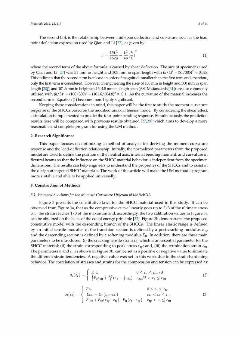
Figure 3 presents the constitutive laws for the SHCC material used in this study. It can beobserved from Figure 3a, that as the compressive curve linearly goes up to 2/3 of the ultimate stressσcu, the strain reaches 1/3 of the maximum and, accordingly, the two calibration values in Figure 3acan be obtained on the basis of the equal energy principle [32]. Figure 3b demonstrates the proposedconstitutive model with the descending branch of the SHCCs. The linear elastic range is definedby an initial tensile modulus E, the transition section is defined by a post-cracking modulus Etc,and the descending section is defined by a softening modulus Etf. In addition, there are three mainparameters to be introduced: (i) the cracking tensile strain εtc which is an essential parameter for theSHCC material; (ii) the strain corresponding to peak stress εtp; and, (iii) the termination strain εtu.The parameters η and µ, as shown in Figure 3b, can be set as a positive or negative value to simulatethe different strain tendencies. A negative value was set in this work due to the strain-hardeningbehavior. The correlation of stresses and strains for the compression and tension can be expressed as:

σc(εc) =

{Ecεc 0 ≤ εc ≤ εcu/313 Ecεcu + λE

4 (εc − 13εcu) εcu/3 < εc ≤ εcu

(2)

σt(εt) =

Eεt 0 ≤ εt ≤ εtc

Eεtc + Etc(ε t−εtc) εtc < εt ≤ εtp

Eεtc + Etc(εtp−εtc)+Etf

(εt−εtp

)εtp < εt ≤ εtu

(3)

Materials 2019, 12, 113 4 of 14

where the stresses and strains are denoted by σc, σt, εc and εt, respectively. Several control parameters,as shown in Figure 3, are normalized by εtc and E, as expressed by:

α =εtp

εtc; βtu =

εtu

εtc; ωcu =

εcu

εtc(4)

λ =Ec

E; η =

Etc

E; µ =

EtfE

(5)

Materials 2018, 11, x FOR PEER REVIEW 4 of 14

The second link is the relationship between mid-span deflection and curvature, such as the load point deflection expression used by Qian and Li [27], as given by:

2 2215 ( )

162ρ 4ρL L hu

L= + (1)

where the second term of the above formula is caused by shear deflection. The size of specimens used by Qian and Li [27] was 51 mm in height and 305 mm in span length with (h/L)2 = (51/305)2 ≈ 0.028. This indicates that the second term is at least an order of magnitude smaller than the first term and, therefore, only the first term is considered. However, in engineering the sizes of 100 mm in height and 300 mm in span length [30]), and 101.6 mm in height and 304.8 mm in length span (ASTM standards [31]) are also commonly utilized with (h/L)2 = (100/300)2 = (101.6/304.8)2 ≈ 0.1. As the curvature of the material increases the second term in Equation Error! Reference source not found. becomes more highly significant.

Keeping these considerations in mind, this paper will be the first to study the moment-curvature response of the SHCCs based on the modified uniaxial tension model. By considering the shear effect, a simulation is implemented to predict the four-point bending response. Simultaneously, the prediction results here will be compared with previous results obtained [27,29] which aims to develop a more reasonable and complete program for using the UM method.

2. Research Significance

This paper focuses on optimizing a method of analysis for deriving the moment-curvature response and the load-deflection relationship. Initially, the normalized parameters from the proposed model are used to define the position of the neutral axis, internal bending moment, and curvature in flexural beams so that the influence on the SHCC material behavior is independent from the specimen dimensions. The results can help engineers to understand the properties of the SHCCs and to assist in the design of targeted SHCC materials. The work of this article will make the UM method’s program more suitable and able to be applied universally.

3. Construction of Methods

3.1. Proposed Solutions for the Moment-Curvature Diagram of the SHCCs

Figure 3. The proposed model of the SHCC in uniaxial tests, (a) stress-strain behavior of SHCC in uniaxial compression; (b) stress-strain behavior of SHCC in uniaxial compression.

Figure 3 presents the constitutive laws for the SHCC material used in this study. It can be observed from Figure 3a, that as the compressive curve linearly goes up to 2/3 of the ultimate stress σcu, the strain reaches 1/3 of the maximum and, accordingly, the two calibration values in Figure 3a can be obtained on the basis of the equal energy principle [32]. Figure 3b demonstrates the proposed constitutive model with the descending branch of the SHCCs. The linear elastic range is defined by an initial tensile modulus 𝐸, the transition section is defined by a post-cracking modulus Etc, and the descending section is defined by a softening modulus Etf. In addition, there are three main parameters

Figure 3. The proposed model of the SHCC in uniaxial tests, (a) stress-strain behavior of SHCC inuniaxial compression; (b) stress-strain behavior of SHCC in uniaxial compression.

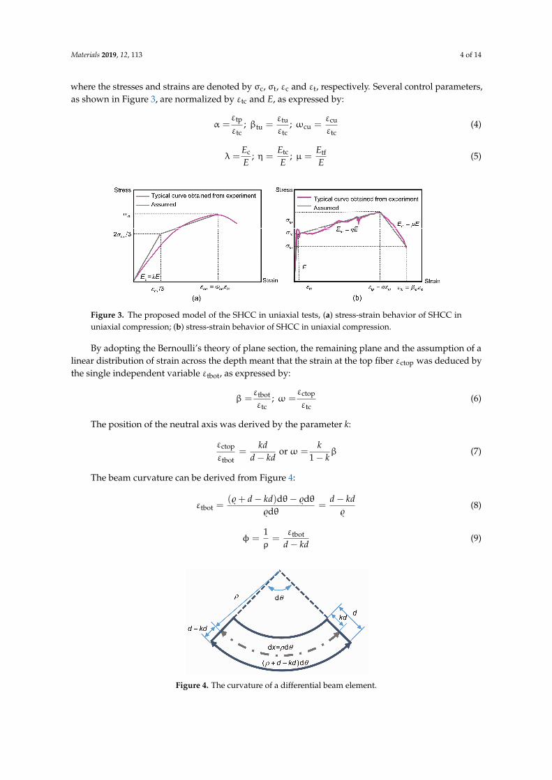
By adopting the Bernoulli’s theory of plane section, the remaining plane and the assumption of alinear distribution of strain across the depth meant that the strain at the top fiber εctop was deduced bythe single independent variable εtbot, as expressed by:

β =εtbotεtc

; ω =εctop

εtc(6)

The position of the neutral axis was derived by the parameter k:

εctop

εtbot=

kdd− kd

orω =k

1− kβ (7)

The beam curvature can be derived from Figure 4:

εtbot =($ + d− kd)dθ− $dθ

$dθ=

d− kd$

(8)

φ =1ρ=

εtbotd− kd

(9)

Materials 2018, 11, x FOR PEER REVIEW 5 of 14

to be introduced: (i) the cracking tensile strain εtc which is an essential parameter for the SHCC material; (ii) the strain corresponding to peak stress εtp; and, (iii) the termination strain εtu. The parameters η and μ, as shown in Figure 3b, can be set as a positive or negative value to simulate the different strain tendencies. A negative value was set in this work due to the strain-hardening behavior. The correlation of stresses and strains for the compression and tension can be expressed as:

c c c cu

c cc cu c cu cu c cu

ε 0 ε ε 3σ (ε ) 1 λ 1ε (ε - ε ) ε 3 ε ε

3 4 3

EEE

≤ ≤=

+ < ≤

(2)

t t tc

t t tc tc t tc tc t tp

tc tc tp tc tf t tp tp t tu

ε 0 ε εσ (ε ) = ε (ε -ε ) ε ε ε

ε (ε -ε )+ (ε -ε ) ε ε ε

EE EE E E

≤ ≤ + < ≤ + < ≤

(3)

where the stresses and strains are denoted by σc, σt, εc and εt, respectively. Several control parameters, as shown in Figure 3, are normalized by εtc and E, as expressed by:

tp tu cutu cu

tc tc tc

ε ε εα = ; β = ; ω =ε ε ε (4)

c tc tfλ = ; η = ; μ =E E EE E E

(5)

By adopting the Bernoulli’s theory of plane section, the remaining plane and the assumption of a linear distribution of strain across the depth meant that the strain at the top fiber εctop was deduced by the single independent variable εtbot, as expressed by:

ctoptbot

tc tc

εεβ = ; ω =

ε ε (6)

The position of the neutral axis was derived by the parameter k:

ctop

tbot

ε= or ω = β

ε 1kd k

d kd k− − (7)

The beam curvature can be derived from Figure 4:

(ρ )dθ ρdθρdθ ρtbot

d kd d kdε+ − − −= = (8)

ϕ = 1ρ = ε𝑑 − 𝑘𝑑 (9)

Figure 4. The curvature of a differential beam element. Figure 4. The curvature of a differential beam element.

Materials 2019, 12, 113 5 of 14

By substituting Equations (4)–(7) into Equations (2) and (3), the normalized stress–strainrelationship can be expressed as:

σc(ω)

Eεtc=

{λω 0 ≤ ω ≤ ωcu/313λωcu + λ

4 (ω−13ωcu

)ωcu/3 < ω ≤ ωcu

(10)

σt(β)

Eεtc=

β 0 ≤ β ≤ 11 + η(β− 1) 1 < β ≤ α1 + η(α− 1) + µ(β− α) α < β ≤ βtu

(11)

Figure 5 presents the distribution of stress and strain based on proposed constitutive models. Clearly,three different stages could be divided according to the parameter β: (i) stage 1 represents the elastic phasewith 0 < β ≤ 1; (ii) stage 2 represents the hardening phase with 1 < β ≤ α; and, (iii) stage 3 representsthe softening phase with α < β < βtu. These stages are shown in Table 1. However, it should be notedthat there were two possible situations for stages 2 and 3 which depended upon the condition of thehighest-compression fiber: (i) the elastic (0≤ω≤ωcu/3); or, (ii) the plastic (ωcu/3≤ω≤ωcu) state.

Materials 2018, 11, x FOR PEER REVIEW 6 of 14

By substituting Equations Error! Reference source not found.–Error! Reference source not found. into Equations Error! Reference source not found. and Error! Reference source not found., the normalized stress–strain relationship can be expressed as:

cuc

tc cu cu cu

λω 0 ω ω 3σ (ω)1 λ 1ε λω + (ω - ω ) 3 ω ω3 4 3 cuE ω

≤ ≤=

< ≤

(10)

t

tctu

β 0 β 1σ (β)

= 1 η(β - 1) 1 β α ε

1 η(α - 1)+μ(β - α) α < β βE

≤ ≤ + < ≤ + ≤

(11)

Figure 5 presents the distribution of stress and strain based on proposed constitutive models. Clearly, three different stages could be divided according to the parameter β: (i) stage 1 represents the elastic phase with 0 < β ≤ 1; (ii) stage 2 represents the hardening phase with 1 < β ≤ α; and, (iii) stage 3 represents the softening phase with α < β < βtu. These stages are shown in Table 1. However, it should be noted that there were two possible situations for stages 2 and 3 which depended upon the condition of the highest-compression fiber: (i) the elastic (0 ≤ ω ≤ ωcu/3); or, (ii) the plastic (ωcu/3 ≤ ω ≤ ωcu) state.

Figure 5. The strain and stress distributions for the different stages with applied normalized tensile strain at the bottom fiber (β).

The values of hi and Yi in Figure 5 can be obtained by explicit integration across the thickness of the compression zone. Taking the example of stage 1 (the force component Fc1 and its lever arm γc1) the integration is expressed as:

c1 c1 c1 c10 0c1

σ ( )d ; σ ( ) dkd kdbF b z z Y z z z

F= = (12)

2c1 c1

tc

λβ 2; ε 2(1 ) 3

F Yk kbdE k d

= =−

(13)

Figure 5. The strain and stress distributions for the different stages with applied normalized tensilestrain at the bottom fiber (β).

The values of hi and Yi in Figure 5 can be obtained by explicit integration across the thickness ofthe compression zone. Taking the example of stage 1 (the force component Fc1 and its lever arm γc1)the integration is expressed as:

Fc1 = b∫ kd

0σc1(z)dz; Yc1 =

bFc1

∫ kd

0σc1(z)zdz (12)

Fc1

bdEεtc=

λβk2

2(1− k);

Yc1

d=

2k3

(13)

Materials 2019, 12, 113 6 of 14

where the parameter z is in the position of εci, calculated from the neutral axis. All heights and leverarms, as shown in Figure 5, were normalized with respect to beam depth d. By solving Equation (14)for static equilibrium in the horizontal direction of the cross section, the axis depth ratio k was obtained:

∑ Fi = 0 (i represents any stage) (14)

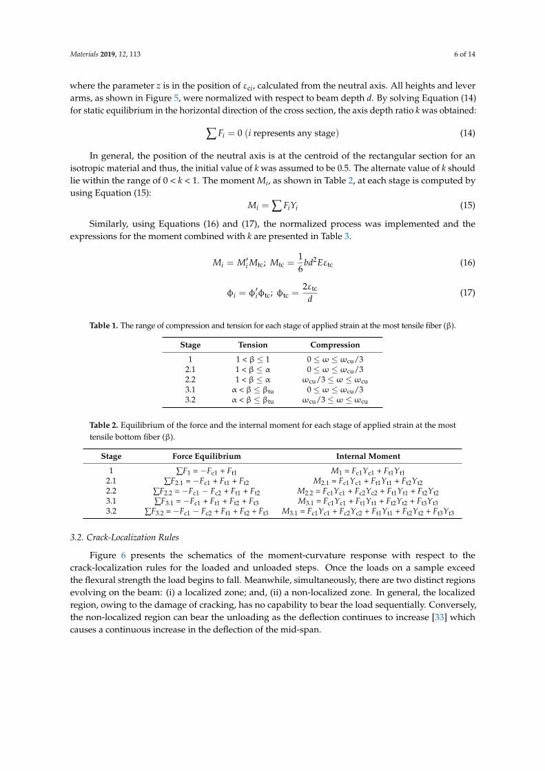
In general, the position of the neutral axis is at the centroid of the rectangular section for anisotropic material and thus, the initial value of k was assumed to be 0.5. The alternate value of k shouldlie within the range of 0 < k < 1. The moment Mi, as shown in Table 2, at each stage is computed byusing Equation (15):

Mi = ∑ FiYi (15)

Similarly, using Equations (16) and (17), the normalized process was implemented and theexpressions for the moment combined with k are presented in Table 3.

Mi = M′i Mtc; Mtc =16

bd2Eεtc (16)

φi = φ′iφtc; φtc =2εtc

d(17)

Table 1. The range of compression and tension for each stage of applied strain at the most tensile fiber (β).

Stage Tension Compression

1 1 < β ≤ 1 0 ≤ ω ≤ ωcu/32.1 1 < β ≤ α 0 ≤ ω ≤ ωcu/32.2 1 < β ≤ α ωcu/3 ≤ ω ≤ ωcu3.1 α < β ≤ βtu 0 ≤ ω ≤ ωcu/33.2 α < β ≤ βtu ωcu/3 ≤ ω ≤ ωcu

Table 2. Equilibrium of the force and the internal moment for each stage of applied strain at the mosttensile bottom fiber (β).

Stage Force Equilibrium Internal Moment

1 ∑F1 = −Fc1 + Ft1 M1 = Fc1Yc1 + Ft1Yt12.1 ∑F2.1 = −Fc1 + Ft1 + Ft2 M2.1 = Fc1Yc1 + Ft1Yt1 + Ft2Yt22.2 ∑F2.2 = −Fc1 − Fc2 + Ft1 + Ft2 M2.2 = Fc1Yc1 + Fc2Yc2 + Ft1Yt1 + Ft2Yt23.1 ∑F3.1 = −Fc1 + Ft1 + Ft2 + Ft3 M3.1 = Fc1Yc1 + Ft1Yt1 + Ft2Yt2 + Ft3Yt33.2 ∑F3.2 =−Fc1 − Fc2 + Ft1 + Ft2 + Ft3 M3.1 = Fc1Yc1 + Fc2Yc2 + Ft1Yt1 + Ft2Yt2 + Ft3Yt3

3.2. Crack-Localization Rules

Figure 6 presents the schematics of the moment-curvature response with respect to thecrack-localization rules for the loaded and unloaded steps. Once the loads on a sample exceedthe flexural strength the load begins to fall. Meanwhile, simultaneously, there are two distinct regionsevolving on the beam: (i) a localized zone; and, (ii) a non-localized zone. In general, the localizedregion, owing to the damage of cracking, has no capability to bear the load sequentially. Conversely,the non-localized region can bear the unloading as the deflection continues to increase [33] whichcauses a continuous increase in the deflection of the mid-span.

Materials 2019, 12, 113 7 of 14

Table 3. Solutions of the neutral-axis depth ratio and normalized moment, and the curvature for eachstage of applied strain at the most tensile fiber (β).

Stage k M′

1 k1 =

{12 for λ = 1−1+

√λ

−1+λ for λ < 1 or λ > 1M′1 =

β[(1−k1)3+λk1

3]3(1−k1)

2.1 k21 = D21−√λβ2D21

D21−λβ2

D21 = ηβ2 − 2ηβ+ η+ 2β− 1

M′21 = C21−3C21k21+3C21k212−(C21+2β3λ)

6(k21−1)β2

C21 = −2 + (1− β)[3− β(−3 + η)− η+ 2β2η]

2.2 k22 = 4D22+3(βλωcu−λωcu2)−2√

3β2λD22

4D22−3(β2λ+2βλωcu+λωcu2)

D22 = −3 + 6β+ 3η− 6βη+ 3β2η+ λωcu2

M′22 =C22−3C22k22+3(C22+81β2λωcu)k2

22−(C22−54β3λ+81β2λωcu)k322

648(k21−1)β2

C22 = 108− 324β2 − 108η+ 324β2η− 216β3η− 19λω3cu

3.1k31 = −D31−

√β2λD31

−D31+β2λ

D31 = −1 + η− α2η+ α2µ+ β2µ+2β[1 + (α − 1)η− αµ]

M′31 =C31+D31−(3C31+2E31)k31+(3C31+2E31)k2

31−(C31−2β3λ)k331

6(1−k31)β2

C31 = 2− 3α2+3β2+3α2η− 3α3η− 3β2η+ 3αβ2η+ 2α3µ

−3α2βµ+ β3µ

E31 = −6β+ 6αβ+ 3βη− 6αβη+ 3α2βη

3.2k32 =

−4D32−3(βλωcu−λω2cu)−2

√3β2λD32

−4D32+3(β2λ−2βλωcu+λω2cu)

D32 = −3− 3(α2−1)η+ 6β[1 + (α − 1)η]+3(α − β)2µ+ λω2

cu

M′32 =C32−3C32k32−(C32+18β3λ−27β2λωcu)k2

32+3(C32−9β2λωcu)k332

216(k32−1)β2

C32 = 36 + 36(α3 − 1)η− 108β2[1 + (α − 1)η]− 36(α− β)2(2α+ β)µ+ λω3cu

Materials 2018, 11, x FOR PEER REVIEW 8 of 14

Table 3. Solutions of the neutral-axis depth ratio and normalized moment, and the curvature for each stage of applied strain at the most tensile fiber (β).

Stage k M’

1 1

1 for λ=12

1+ λ for λ<1 or λ>11+λ

k

=

− −

3 31 1

11

β (1 ) λ'

3(1 )

k kM

k

− + =−

2.1

221 21

21 221

221

λβλβ

β 2ηβ + η + 2β 1

D Dk

DD η

−=

−= − −

2 3

21 21 21 21 21 2121 2

212

21

3 3 ( 2β λ)'

6( 1)2 (1 β)[3 β( 3 η) η + 2β η]

C C k C k CM

k βC

− + − +=

−= − + − − − + −

2.2

2 222 cu cu 22

22 2 222 cu cu

2 222 cu

4 3(βλω λω ) 2 3β λ4 3(β λ + 2βλω + λω )

3 6β 3η 6βη 3β η + λω

D Dk

DD

+ − −=

−= − + + − +

2 2 3 2 322 22 22 22 cu 22 22 cu 22

22 221

2 2 3 322 cu

3 +3( +81β λω ) ( 54β λ +81β λω )'

648( 1)β108 324β 108η + 324β η 216β η 19λω

C C k C k C kM

kC

− − −=

−= − − − −

3.1

231 31

31 231

2 2 231

β λβ λ

1 η α η + α μ + β μ +2β[1 + (α 1)η αμ]

D Dk

DD

− −=

− += − + −

− −

2 3 331 31 31 31 31 31 31 31 31 31

31 231

2 2 2 3 2 2 331

2 3

231

+ (3 + 2 ) + (3 + 2 ) ( 2β λ)'

6(1 )β2 3α + 3β + 3α η 3α η 3β η + 3αβ η + 2α μ

3α βμ + β μ6β 6αβ + 3βη 6αβη + 3α βη

C D C E k C E k C kM

kC

E

− − −=

−= − − −

−= − + −

3.2

2 232 cu cu 32

32 2 232 cu cu

232

2 2cu

4 3(βλω λω ) 2 3β λ4 3(β λ 2βλω +λω )

3 3(α -1)η + 6β[1 + (α 1)η] +3(α β) μ + λω

D Dk

DD

− − − −=

− + −= − − −−

3 2 2 2 332 32 32 32 cu 32 32 cu 32

32 232

3 2 2 332 cu

3 ( +18β λ 27β λω ) +3( 9β λω )'

216( 1)β36 36(α 1)η 108β [1+ (α 1)η] 36(α β) (2α+ β)μ+ λω

C C k C k C kM

kC

− − − −=

−= + − − − − −

Figure 6. The moment-curvature response and the crack localization rules. Inset: schematic of a four-point bending test (only left half of the model is shown).

The inset of Figure 6 shows the schematic diagram of a four-point bending test. It is observed that a localized zone occurs in the mid-span while the location of the crack is random. In order to describe the localized zone behavior, in terms of the stress-strain relationship instead of a stress-cracking response, it is assumed that the main cracks are smeared uniformly over the mid-section zone. The length of the smeared-crack zone is defined as cL and the range of c is 0 ≤ c ≤ 1/6, where L is the clear span. Assuming a default value of c = 1/6, this signifies that the cracks are smeared over the entire mid-span.

Dividing the moment-curvature response diagram, as shown in Figure 6, into three portions: (i) an ascending portion from 0 to Mtc which corresponds to the elastic response with a unique path of loading and unloading; (ii) a non-elastic ascending portion from Mtc to Mmax. Any point included in this portion of the curve indicates the beginning of unloading and the unloading stiffness is consistent with the elastic stiffness; and, (iii) the descending portion from Mmax to Mfail.

For each loading step the moment and the subsequent curvature along the entire length of the beam are calculated by solving the static balanced equation. Once the loading exceeds the maximum value, the curvature in the cracked region is based upon the descending portion from 𝑀 to 𝑀 . In the uncracked region, the curvature decreases linearly and elastically during unloading where M <

Figure 6. The moment-curvature response and the crack localization rules. Inset: schematic of afour-point bending test (only left half of the model is shown).

The inset of Figure 6 shows the schematic diagram of a four-point bending test. It is observed that alocalized zone occurs in the mid-span while the location of the crack is random. In order to describe thelocalized zone behavior, in terms of the stress-strain relationship instead of a stress-cracking response,it is assumed that the main cracks are smeared uniformly over the mid-section zone. The length ofthe smeared-crack zone is defined as cL and the range of c is 0 ≤ c ≤ 1/6, where L is the clear span.Assuming a default value of c = 1/6, this signifies that the cracks are smeared over the entire mid-span.

Dividing the moment-curvature response diagram, as shown in Figure 6, into three portions:(i) an ascending portion from 0 to Mtc which corresponds to the elastic response with a unique path ofloading and unloading; (ii) a non-elastic ascending portion from Mtc to Mmax. Any point included inthis portion of the curve indicates the beginning of unloading and the unloading stiffness is consistentwith the elastic stiffness; and, (iii) the descending portion from Mmax to Mfail.

For each loading step the moment and the subsequent curvature along the entire length of thebeam are calculated by solving the static balanced equation. Once the loading exceeds the maximumvalue, the curvature in the cracked region is based upon the descending portion from Mmax to M f ail .In the uncracked region, the curvature decreases linearly and elastically during unloading whereM < Mtc. If the section load exceeds Mtc, the unloading curvature of the cracked area will beaccompanied by a quasi-linear recovery path expressed as:

φi = φj−1 − ξ(Mj−1 −Mj)

EI(18)

where φj−1 and Mj−1 represent the previous state of the curvature and moment, respectively. Both φiand Mj are the current states. The unloading factor is 0 < ζ < 1, ζ = 1 and signifies unloading withinitial elastic stiffness. When ζ = 0, this indicates no curvature recovery during unloading, which is thesituation assumed in the present work.

Materials 2019, 12, 113 8 of 14

3.3. Procedures to Obtain the Load-Deflection Behavior from a Four-Point Bending Test

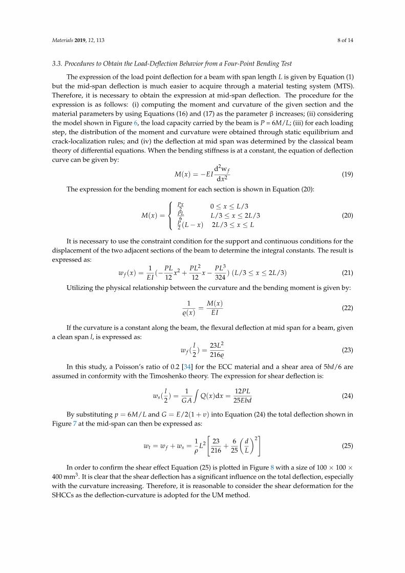
The expression of the load point deflection for a beam with span length L is given by Equation (1)but the mid-span deflection is much easier to acquire through a material testing system (MTS).Therefore, it is necessary to obtain the expression at mid-span deflection. The procedure for theexpression is as follows: (i) computing the moment and curvature of the given section and thematerial parameters by using Equations (16) and (17) as the parameter β increases; (ii) consideringthe model shown in Figure 6, the load capacity carried by the beam is P = 6M/L; (iii) for each loadingstep, the distribution of the moment and curvature were obtained through static equilibrium andcrack-localization rules; and (iv) the deflection at mid span was determined by the classical beamtheory of differential equations. When the bending stiffness is at a constant, the equation of deflectioncurve can be given by:

M(x) = −EId2w f

dx2 (19)

The expression for the bending moment for each section is shown in Equation (20):

M(x) =

Px2 0 ≤ x ≤ L/3

PL6 L/3 ≤ x ≤ 2L/3

P2 (L− x) 2L/3 ≤ x ≤ L

(20)

It is necessary to use the constraint condition for the support and continuous conditions for thedisplacement of the two adjacent sections of the beam to determine the integral constants. The result isexpressed as:

w f (x) =1

EI(−PL

12x2 +

PL2

12x− PL3

324) (L/3 ≤ x ≤ 2L/3) (21)

Utilizing the physical relationship between the curvature and the bending moment is given by:

1$(x)

=M(x)

EI(22)

If the curvature is a constant along the beam, the flexural deflection at mid span for a beam, givena clean span l, is expressed as:

w f (l2) =

23L2

216$(23)

In this study, a Poisson’s ratio of 0.2 [34] for the ECC material and a shear area of 5bd/6 areassumed in conformity with the Timoshenko theory. The expression for shear deflection is:

ws(l2) =

1GA

∫Q(x)dx =

12PL25Ebd

(24)

By substituting p = 6M/L and G = E/2(1 + υ) into Equation (24) the total deflection shown inFigure 7 at the mid-span can then be expressed as:

wt = w f + ws =1ρ

L2

[23

216+

625

(dL

)2]

(25)

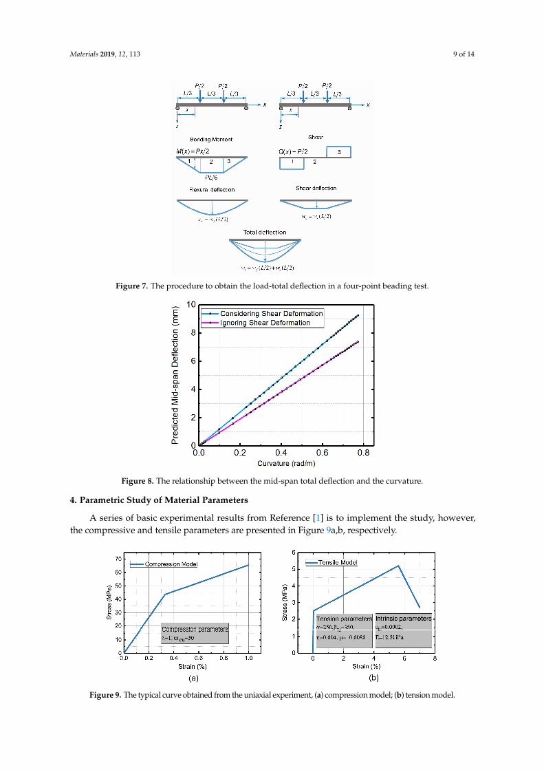
In order to confirm the shear effect Equation (25) is plotted in Figure 8 with a size of 100 × 100 ×400 mm3. It is clear that the shear deflection has a significant influence on the total deflection, especiallywith the curvature increasing. Therefore, it is reasonable to consider the shear deformation for theSHCCs as the deflection-curvature is adopted for the UM method.

Materials 2019, 12, 113 9 of 14

Materials 2018, 11, x FOR PEER REVIEW 10 of 14

1 12( ) ( )d2 25sl PLw Q x x

GA Ebd= = (24)

By substituting 𝑝 = 6 𝑀 𝐿⁄ and 𝐺 = 𝐸 2(1 + 𝜐)⁄ into Equation Error! Reference source not found. the total deflection shown in Figure 7 at the mid-span can then be expressed as:

221 23 6

216 25t f sdw w w L

ρ L

= + = +

(25)

Figure 7. The procedure to obtain the load-total deflection in a four-point beading test.

In order to confirm the shear effect Equation Error! Reference source not found. is plotted in Figure 8 with a size of 100 × 100 × 400 mm3. It is clear that the shear deflection has a significant influence on the total deflection, especially with the curvature increasing. Therefore, it is reasonable to consider the shear deformation for the SHCCs as the deflection-curvature is adopted for the UM method.

Figure 8. The relationship between the mid-span total deflection and the curvature.

4. Parametric Study of Material Parameters

Figure 7. The procedure to obtain the load-total deflection in a four-point beading test.

Materials 2018, 11, x FOR PEER REVIEW 10 of 14

1 12( ) ( )d2 25sl PLw Q x x

GA Ebd= = (24)

By substituting 𝑝 = 6 𝑀 𝐿⁄ and 𝐺 = 𝐸 2(1 + 𝜐)⁄ into Equation Error! Reference source not found. the total deflection shown in Figure 7 at the mid-span can then be expressed as:

221 23 6

216 25t f sdw w w L

ρ L

= + = +

(25)

Figure 7. The procedure to obtain the load-total deflection in a four-point beading test.

In order to confirm the shear effect Equation Error! Reference source not found. is plotted in Figure 8 with a size of 100 × 100 × 400 mm3. It is clear that the shear deflection has a significant influence on the total deflection, especially with the curvature increasing. Therefore, it is reasonable to consider the shear deformation for the SHCCs as the deflection-curvature is adopted for the UM method.

Figure 8. The relationship between the mid-span total deflection and the curvature.

4. Parametric Study of Material Parameters

Figure 8. The relationship between the mid-span total deflection and the curvature.

4. Parametric Study of Material Parameters

A series of basic experimental results from Reference [1] is to implement the study, however,the compressive and tensile parameters are presented in Figure 9a,b, respectively.

Materials 2018, 11, x FOR PEER REVIEW 11 of 14

A series of basic experimental results from Reference [1] is to implement the study, however, the compressive and tensile parameters are presented in Figure 9a,b, respectively.

Figure 9. The typical curve obtained from the uniaxial experiment, (a) compression model; (b)

tension model.

Figure 10a–e shows the normalized moment-curvature responses with the parameters of α, η, μ, and λ with the influence of the tensile parameters discussed first. Figure 10a demonstrates that the parameter α has a significant effect on the peak strength and ductility. As the transition strain α increases, both flexural strength and ductility raise linearly. The impact on the parameter η is shown in Figure 10b. It is observed that the ultimate strength is quite sensitive to the variations in η but it differs from the influence of parameter α. When the value of η increases, its peak strength increases with an enhancing stiffness. Figure 10c demonstrates that the change in the μ value has little effect on the peak strength but has a significant effect on the post-peak response. Like the tensile parameters, the compressive materials λ and ωcu are also studied in Figure 10d,e.

Figure 9. The typical curve obtained from the uniaxial experiment, (a) compression model; (b) tension model.

Materials 2019, 12, 113 10 of 14

Figure 10a–e shows the normalized moment-curvature responses with the parameters of α, η,µ, and λ with the influence of the tensile parameters discussed first. Figure 10a demonstrates thatthe parameter α has a significant effect on the peak strength and ductility. As the transition strain αincreases, both flexural strength and ductility raise linearly. The impact on the parameter η is shownin Figure 10b. It is observed that the ultimate strength is quite sensitive to the variations in η but itdiffers from the influence of parameter α. When the value of η increases, its peak strength increaseswith an enhancing stiffness. Figure 10c demonstrates that the change in the µ value has little effect onthe peak strength but has a significant effect on the post-peak response. Like the tensile parameters,the compressive materials λ andωcu are also studied in Figure 10d,e.

Materials 2018, 11, x FOR PEER REVIEW 11 of 14

A series of basic experimental results from Reference [1] is to implement the study, however, the compressive and tensile parameters are presented in Figure 9a,b, respectively.

Figure 9. The typical curve obtained from the uniaxial experiment, (a) compression model; (b)

tension model.

Figure 10a–e shows the normalized moment-curvature responses with the parameters of α, η, μ, and λ with the influence of the tensile parameters discussed first. Figure 10a demonstrates that the parameter α has a significant effect on the peak strength and ductility. As the transition strain α increases, both flexural strength and ductility raise linearly. The impact on the parameter η is shown in Figure 10b. It is observed that the ultimate strength is quite sensitive to the variations in η but it differs from the influence of parameter α. When the value of η increases, its peak strength increases with an enhancing stiffness. Figure 10c demonstrates that the change in the μ value has little effect on the peak strength but has a significant effect on the post-peak response. Like the tensile parameters, the compressive materials λ and ωcu are also studied in Figure 10d,e.

Materials 2018, 11, x FOR PEER REVIEW 12 of 14

Figure 10. Parametric studies of the five material parameters on the normalized moment curvature response: (a) vary α; (b) vary η; (c) vary μ; (d) vary λ and (e) vary ωcu

The parameter λ represents the ratio between the compression elastic modulus and the tension elastic modulus. As the ratio increases, the peak value increases while the ductility decreases slightly, as shown in Figure 10d. The effect of the ωcu variation on the peak strength and ductility is demonstrated in Figure 10e. It is clear that the effect of ωcu on the bending response is extremely small. Comparing this with the effect of tensile parameters, the influence caused by the change of compression parameters is relatively insignificant.

5. Simulation and Discussion

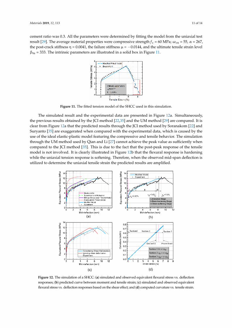
The SHCCs employed in this study were polyethylene fibers with 2% volume fraction. The mix ratio was 1:0.75:0.1:0.02 by weight (cement: sand: silica fume: super plasticizer). The water to cement ratio was 0.3. All the parameters were determined by fitting the model from the uniaxial test result [29]. The average material properties were compressive strength fc = 60 MPa; ωcu = 55, α = 267, the post-crack stiffness η = 0.0041, the failure stiffness μ = −0.0144, and the ultimate tensile strain level βtu = 333. The intrinsic parameters are illustrated in a solid box in Figure 11.

Figure 11. The fitted tension model of the SHCC used in this simulation.

The simulated result and the experimental data are presented in Figure 12a. Simultaneously, the previous results obtained by the JCI method [22,35] and the UM method [29] are compared. It is clear from Figure 12a that the predicted results through the JCI method used by Soranakom [22] and Suryanto [35] are exaggerated when compared with the experimental data, which is caused by the use of the ideal elastic-plastic model featuring the compressive and tensile behavior. The simulation through the UM method used by Qian and Li [27] cannot achieve the peak value as sufficiently when compared to the JCI method [35]. This is due to the fact that the post-peak response of the tensile model is not involved. It is clearly illustrated in Figure 12b that the flexural response is hardening while the uniaxial tension response is softening. Therefore, when the observed mid-span deflection is utilized to determine the uniaxial tensile strain the predicted results are amplified.

Figure 10. Parametric studies of the five material parameters on the normalized moment curvatureresponse: (a) vary α; (b) vary η; (c) vary µ; (d) vary λ and (e) varyωcu

The parameter λ represents the ratio between the compression elastic modulus and the tensionelastic modulus. As the ratio increases, the peak value increases while the ductility decreasesslightly, as shown in Figure 10d. The effect of the ωcu variation on the peak strength and ductilityis demonstrated in Figure 10e. It is clear that the effect ofωcu on the bending response is extremelysmall. Comparing this with the effect of tensile parameters, the influence caused by the change ofcompression parameters is relatively insignificant.

5. Simulation and Discussion

The SHCCs employed in this study were polyethylene fibers with 2% volume fraction. The mixratio was 1:0.75:0.1:0.02 by weight (cement: sand: silica fume: super plasticizer). The water to

Materials 2019, 12, 113 11 of 14

cement ratio was 0.3. All the parameters were determined by fitting the model from the uniaxial testresult [29]. The average material properties were compressive strength f c = 60 MPa;ωcu = 55, α = 267,the post-crack stiffness η = 0.0041, the failure stiffness µ = −0.0144, and the ultimate tensile strain levelβtu = 333. The intrinsic parameters are illustrated in a solid box in Figure 11.

Materials 2018, 11, x FOR PEER REVIEW 12 of 14

Figure 10. Parametric studies of the five material parameters on the normalized moment curvature response: (a) vary α; (b) vary η; (c) vary μ; (d) vary λ and (e) vary ωcu

The parameter λ represents the ratio between the compression elastic modulus and the tension elastic modulus. As the ratio increases, the peak value increases while the ductility decreases slightly, as shown in Figure 10d. The effect of the ωcu variation on the peak strength and ductility is demonstrated in Figure 10e. It is clear that the effect of ωcu on the bending response is extremely small. Comparing this with the effect of tensile parameters, the influence caused by the change of compression parameters is relatively insignificant.

5. Simulation and Discussion

The SHCCs employed in this study were polyethylene fibers with 2% volume fraction. The mix ratio was 1:0.75:0.1:0.02 by weight (cement: sand: silica fume: super plasticizer). The water to cement ratio was 0.3. All the parameters were determined by fitting the model from the uniaxial test result [29]. The average material properties were compressive strength fc = 60 MPa; ωcu = 55, α = 267, the post-crack stiffness η = 0.0041, the failure stiffness μ = −0.0144, and the ultimate tensile strain level βtu = 333. The intrinsic parameters are illustrated in a solid box in Figure 11.

Figure 11. The fitted tension model of the SHCC used in this simulation.

The simulated result and the experimental data are presented in Figure 12a. Simultaneously, the previous results obtained by the JCI method [22,35] and the UM method [29] are compared. It is clear from Figure 12a that the predicted results through the JCI method used by Soranakom [22] and Suryanto [35] are exaggerated when compared with the experimental data, which is caused by the use of the ideal elastic-plastic model featuring the compressive and tensile behavior. The simulation through the UM method used by Qian and Li [27] cannot achieve the peak value as sufficiently when compared to the JCI method [35]. This is due to the fact that the post-peak response of the tensile model is not involved. It is clearly illustrated in Figure 12b that the flexural response is hardening while the uniaxial tension response is softening. Therefore, when the observed mid-span deflection is utilized to determine the uniaxial tensile strain the predicted results are amplified.

Figure 11. The fitted tension model of the SHCC used in this simulation.

The simulated result and the experimental data are presented in Figure 12a. Simultaneously,the previous results obtained by the JCI method [22,35] and the UM method [29] are compared. It isclear from Figure 12a that the predicted results through the JCI method used by Soranakom [22] andSuryanto [35] are exaggerated when compared with the experimental data, which is caused by theuse of the ideal elastic-plastic model featuring the compressive and tensile behavior. The simulationthrough the UM method used by Qian and Li [27] cannot achieve the peak value as sufficiently whencompared to the JCI method [35]. This is due to the fact that the post-peak response of the tensilemodel is not involved. It is clearly illustrated in Figure 12b that the flexural response is hardeningwhile the uniaxial tension response is softening. Therefore, when the observed mid-span deflection isutilized to determine the uniaxial tensile strain the predicted results are amplified.

Materials 2018, 11, x FOR PEER REVIEW 13 of 14

Figure 12. The simulation of a SHCC: (a) simulated and observed equivalent flexural stress vs. deflection responses; (b) predicted curve between moment and tensile strain; (c) simulated and observed equivalent flexural stress vs. deflection responses based on the shear effect; and (d) computed curvature vs tensile strain.

In addition, by assuming a complete tensile model, as shown by the dashed rectangle in Figure 11, the softening section of the bending response is also predicted in Figure 12c. The predicted curve displays agreement in all phases of the flexural behavior. Figure 12c depicts another meaningful simulation result based on the shear influence. By considering the shear deflection, this produces a greater consistency with the experimental data. The computed curvature is presented in Figure 12d. It is clear that as the tensile strain enters the softening stage (stage 3) the curvature of the beam is still increasing which also confirms that the post-peak response of tension has a significant impact on the flexural behavior of the SHCCs.

6. Summary and Future Work

This paper presents the solutions for generating load-deflection diagrams of SHCCs. The specific conclusions are drawn as follows:

• The parametric study reveals that the tensile parameters mainly dominate the flexural performance in the moment-curvature diagram. Specifically, the transition strain 𝛼 and post-cracking tensile stiffness η have a direct influence on the peak flexural strength, and the failure stiffness μ has a vital impact on post-peak response. Compared to the tension parameters, the influence of compressive parameters on bending behavior is insignificant.

• The calculation of mid-deflection is affected by the shear effect which depends upon the ratio of specimen’s height to span length. Generally, when the specimen size is 100 × 100 × 400 mm3 or 76.2 × 101.6 × 355.6 mm3 the expression of deflection requires it to take the term into account caused by the shear deflection.

• The predicted load-deflection curve, based upon considering shear effect and post-peak response, presents reasonable consistency when compared with the experiment results under a four point-bending test, especially in the peak and softening portions. The results help to form

Figure 12. The simulation of a SHCC: (a) simulated and observed equivalent flexural stress vs. deflectionresponses; (b) predicted curve between moment and tensile strain; (c) simulated and observed equivalentflexural stress vs. deflection responses based on the shear effect; and (d) computed curvature vs. tensile strain.

Materials 2019, 12, 113 12 of 14

In addition, by assuming a complete tensile model, as shown by the dashed rectangle in Figure 11,the softening section of the bending response is also predicted in Figure 12c. The predicted curvedisplays agreement in all phases of the flexural behavior. Figure 12c depicts another meaningfulsimulation result based on the shear influence. By considering the shear deflection, this produces agreater consistency with the experimental data. The computed curvature is presented in Figure 12d.It is clear that as the tensile strain enters the softening stage (stage 3) the curvature of the beam is stillincreasing which also confirms that the post-peak response of tension has a significant impact on theflexural behavior of the SHCCs.

6. Summary and Future Work

This paper presents the solutions for generating load-deflection diagrams of SHCCs. The specificconclusions are drawn as follows:

• The parametric study reveals that the tensile parameters mainly dominate the flexuralperformance in the moment-curvature diagram. Specifically, the transition strain α andpost-cracking tensile stiffness η have a direct influence on the peak flexural strength, and thefailure stiffness µ has a vital impact on post-peak response. Compared to the tension parameters,the influence of compressive parameters on bending behavior is insignificant.

• The calculation of mid-deflection is affected by the shear effect which depends upon the ratio ofspecimen’s height to span length. Generally, when the specimen size is 100 × 100 × 400 mm3 or76.2 × 101.6 × 355.6 mm3 the expression of deflection requires it to take the term into accountcaused by the shear deflection.

• The predicted load-deflection curve, based upon considering shear effect and post-peak response,presents reasonable consistency when compared with the experiment results under a fourpoint-bending test, especially in the peak and softening portions. The results help to form areasonable procedure for using the UM method which is utilized to determine the tensile behaviorof the SHCCs accurately.

Although the present simulations show a good consistency with the experimental results, it isstill not enough to put the UM method into application. This indicates that the deflection-tensilestrain curve needs to be established with a large number of test data and this process is intended to beimplemented in future work by the author.

Author Contributions: Conceptualization, Z.Q. and Z.H.; Methodology, Z.Q.; Resources, H.L.; Writing-OriginalDraft Preparation, W.C.; Writing-Review & Editing, Z.Q.; Visualization, H.L.; Supervision, Z.H.; ProjectAdministration, Z.H.; Funding Acquisition, Z.H.

Funding: This research was funded by the Zhejiang Provincial Important Research Project of China (No. 2018C03029)and the Zhejiang Provincial Transportation Science and Technology project of China (No. 2018QNA4023).

Acknowledgments: The authors would like to thank the Journal of Zhejiang University-SCIENCE A for checkingthe spelling of the manuscript.

Conflicts of Interest: The authors declare no conflict of interest.

References

1. Li, V.C.; Mishra, D.K.; Wu, H.C. Matrix design for pseudo-strain-hardening fibre reinforced cementitiouscomposites. Mater. Struct. 1995, 28, 586–595. [CrossRef]

2. Qian, S.; Zhou, J.; De Rooij, M.R.; Schlangen, E.; Ye, G.; Van Breugel, K. Self-healing behavior of strain hardeningcementitious composites incorporating local waste materials. Cem. Concr. Compos. 2009, 31, 613–621. [CrossRef]

3. Yu, K.; Wang, Y.; Yu, J.; Xu, S. A strain-hardening cementitious composites with the tensile capacity up to 8%.Constr. Build. Mater. 2017, 137, 410–419. [CrossRef]

4. Kang, J.; Bolander, J.E. Multiscale modeling of strain-hardening cementitious composites. Mech. Res. Commun.2016, 78, 47–54. [CrossRef]

Materials 2019, 12, 113 13 of 14

5. Li, V.C. From micromechanics to structural engineering-the design of cementitous composites for civilengineering applications. JSCE J. Struct. Mech. Earthq. Eng. 1993, 10, 37–48.

6. Herbert, E.N.; Li, V.C. Self-healing of micro cracks in engineered cementitious composites (ECC) under anatural environment. Materials 2013, 6, 2831–2845. [CrossRef]

7. Yun, M.L.; Li, V.C. Durable repair of aged infrastructures using trapping mechanism of engineeredcementitious composites. Cem. Concr. Compos. 1997, 19, 373–385. [CrossRef]

8. Kamada, T.; Li, V.C. The effects of surface preparation on the fracture behavior of ECC/concrete repairsystem. Cem. Concr. Compos. 2000, 22, 423–431. [CrossRef]

9. Lepech, M.D.; Li, V.C. Application of ECC for bridge deck link slabs. Mater. Struct. 2009, 42, 1185. [CrossRef]10. Kim, Y.Y.; Fischer, G.; Li, V.C. Performance of bridge deck link slabs designed with ductile engineered

cementitious composite. Struct. J. 2004, 101, 792–801. [CrossRef]11. Fukuyama, H.; Suwada, H.J. Experimental response of HPFRCC dampers for structural control. J. Adv.

Concr. Technol. 2003, 1, 317–326. [CrossRef]12. Zhu, Z.; Wang, W. Experimental study on mechanical behaviour of circular reinforced concrete columns

strengthened with FRP textile and ECC. J. Southeast Univ. Nat. Sci. Ed. 2016, 5, 031.13. Zheng, Y.-Z.; Wang, W.W.; Brigham, J.C. Flexural behaviour of reinforced concrete beams strengthened with

a composite reinforcement layer: BFRP grid and ECC. Constr. Build. Mater. 2016, 115, 424–437. [CrossRef]14. Ma, H.; Qian, S.; Zhang, Z.; Lin, Z.; Li, V.C. Tailoring engineered cementitious composites with local

ingredients. Constr. Build. Mater. 2015, 101, 584–595. [CrossRef]15. Pan, Z.; Wu, C.; Liu, J.; Wang, W.; Liu, J. Study on mechanical properties of cost-effective polyvinyl alcohol

engineered cementitious composites (PVA-ECC). Constr. Build. Mater. 2015, 78, 397–404. [CrossRef]16. Wang, S.; Li, V.C. Engineered cementitious composites with high-volume fly ash. ACI Mater. J. 2007, 104, 233–241.

[CrossRef]17. Zhou, Y.; Xi, B.; Yu, K.; Sui, L.; Xing, F. Mechanical properties of hybrid ultra-high performance engineered

cementitous composites incorporating steel and polyethylene fibers. Materials 2018, 11, 1448. [CrossRef][PubMed]

18. Wang, S.; Li, V.C. Tailoring of pre-existing flaws in ECC matrix for saturated strain hardening. In Proceedingsof the FRAMCOS-5, Vail, CO, USA, 12–16 April 2004; pp. 1005–1012.

19. Li, V.C.; Wu, H.C.; Maalej, M.; Mishra, D.K.; Hashida, T. Tensile behavior of cement-based composites withrandom discontinuous steel fibers. J. Am. Ceram. Soc. 2010, 79, 74–78. [CrossRef]

20. Kanakubo, T. Tensile characteristics evaluation method for ductile fiber-reinforced cementitious composites.J. Adv. Concr. Technol. 2006, 4, 3–17. [CrossRef]

21. Kanda, T.; Kanakubo, T.; Nagai, S.; Maruta, M. Technical consideration in producing ECC pre-cast structuralelement. In Proceedings of the International RILEM Workshop on High Performance Fiber Reinforced CementitiousComposites in Structural Applications; RILEM Publications SARL: Paris, France, 2006; pp. 229–242.

22. Soranakom, C.; Mobasher, B. Correlation of tensile and flexural responses of strain softening and strainhardening cement composites. Cem. Concr. Compos. 2008, 30, 465–477. [CrossRef]

23. Soranakom, C.; Mobasher, B. Closed-form moment-curvature expressions for homogenized fiber-reinforcedconcrete. ACI Mater. J. 2007, 104, 351–359.

24. Lopez, J.A.; Serna, P.; Navarro-Gregori, J.; Camacho, E. An inverse analysis method based on deflection tocurvature transformation to determine the tensile properties of UHPFRC. Mater. Struct. 2015, 48, 3703–3718.[CrossRef]

25. Ostergaard, L.; Walter, R.; Olesen, J.F. Method for determination of tensile properties of engineeredcementitious composites (ECC). In Proceedings of the 3rd International Conference on ConstructionMaterials, Vancouver, BC, Canada, 22–24 August 2005.

26. Paegle, I.; Minelli, F.; Fischer, G. Cracking and load-deformation behavior of fiber reinforced concrete:Influence of testing method. Cem. Concr. Compos. 2016, 73, 147–163. [CrossRef]

27. Qian, S.; Li, V.C. Simplified inverse method for determining the tensile strain capacity of strain hardeningcementitious composites. J. Adv. Concr. Technol. 2008, 5, 235–246. [CrossRef]

28. Qian, S.; Li, V.C. Simplified inverse method for determining the tensile properties of strain hardeningcementitious composites (SHCC). J. Adv. Concr. Technol. 2008, 6, 353–363. [CrossRef]

29. Maalej, M.; Li, V.C. Flexural/tensile strength ratio in engineered cementitious composites. J. Mater. Civ. Eng.1994, 6, 513–528. [CrossRef]

Materials 2019, 12, 113 14 of 14

30. Method of Test for Bending Moment-Curvature Curve of Fiber-Reinforced Cementitious Composites2007–Jci-S-003-2007; Japanese Concrete Institute Standard Committee: Tokyo, Japan, 2007.

31. ASTM C1609/C1609M-05. Standard Test Method for Flexural Performance of Fiber-Reinforced Concrete (UsingBeam with Third-Point Loading); ASTM International: West Conshohocken, PA, USA, 2005.

32. Fischer, G.D. Deformation Behavior of Reinforced ECC Flexural Members under Reversed Cyclic LoadingConditions. Ph.D. Dissertation, University of Michigan, Ann Arbor, MI, USA, 2002.

33. Hillerborg, A. Analysis of fracture by means of the fictitious crack model, particularly for fiber reinforcedconcrete. Int. J. Cem. Compos. 1980, 2, 177–184.

34. Rossi, P. Ultra-high-performance fiber-reinforced concretes. Concr. Int. 2001, 23, 1216–1221.35. Suryanto, B.; Reynaud, R.; Cockburn, B. Sectional analysis of engineered cementitious composite beams.

Mag. Concr. Res. 2018, 70, 1135–1148. [CrossRef]

© 2018 by the authors. Licensee MDPI, Basel, Switzerland. This article is an open accessarticle distributed under the terms and conditions of the Creative Commons Attribution(CC BY) license (http://creativecommons.org/licenses/by/4.0/).