INTERNATIONAL UNION OF THEORETICAL

AND APPLIED MECHANICS

STRESS WAVES

IN ANELASTIC SOLIDSSYMPOSIUM

HELD AT BROWN UNIVERSITY, PROVIDENCE, R. I.

APRIL 3-5, 1963

EDITORS

HERBERT KOLSKY WILLIAM PRAGERII UOW IN UN IVE RS1 TV I Jl M - l'O R 3 C H U N C B LA II 0 RATO1UUM

PROVIDENCE, It. I., U.S.A. /.(JIUCII, 8CHW15IZ

WITH 145 FIGURES

SPRINGER-VERLAGBE RLIN/GOTTIN GEN/HEIDELBERG

1964

Propagation of Magneto elastic Disturbancesin Viscoelastic Bodies

By Sylwcster Kaliski and Witold Nowacki

Polish Academy of Sciences, Warsaw, Poland

1. Introduction

In the present paper, we formulate the equations of magnetovisco-olasticity and appropriate boundary conditions for a linearly visco-elastic medium with finite conductivity. In particular, we shall considerthe boundary conditions for an ideal medium, that is perfectly elasticand perfectly conductive.

In magnetohydrodynamics, the boundary conditions on the surfacewhose normal is parallel to the vector of the initial magnetic field,assume different forms depending on the manner in which the transitionto vanishing mechanical and magnetic viscosities is effected [1, 2].

The same problem arises in magnetoviscoelasticity for the variousmodels of viscoelastic bodies. In particular, the boundary conditions onthe contact surface of a liquid, and solid body must be discussed.

If, in a boundary problem which concerns the contact of a, liquidand a solid body, we start with the equations of the ideal liquid andthe elastic solid, and assume perfect conductivity of both media, weobtain a unique form of the boundary conditions. Surface waves on thecontact surface of a liquid and a solid were discussed in this mannerin [3].

If, on the other hand, we start with the equations for viscous mediawith finite conductivity and then pass to the limits corresponding tothe elastic body and the ideal liquid of perfect conductivity, we obtaindifferent forms of the boundary conditions, which depend on the mannerin which the transition to vanishing mechanical and magnetic viscositieshas been effected.

In Section 2 of this paper we present general and simplified equationsfor conductors with finite electric conductivity. Section 3 is devotedto general boundary conditions, while Section 4 deals with the transitionto the ideal elastic conductor. In Section 5, we present the forms of thelimit passage for different models and for contact between a liquid anda solid when the magnetic field vector is normal to the contact surface.

44 SYLWESTEB KALISKI and AVITOLD NOWACKI

Finally, in Section 6, we consider a simple example of the transmissionof an elastic wave through the contact surface of the two media undervarious types of boundary conditions.

2. General Equations

Let us consider a linear viscoelastic medium with finite electric con-ductivity and suppose that an initial magnetic field exists in this medium.The action of body forces and external loads produces not only a de-formation field but also a coupled electromagnetic field. We assume thatthe medium is isotropic and homogeneous and disregard the coupledthermal effects as well as the effects of the relaxation of the magneticand electric induction. These effects have been considered in [4, 5].

The points of departure of our consideration are the equations ofmagneto-viseoelasticity which after being linearized [5] assume thefollowing form:

J

div/t =0, divfl =0,

t

/{<*(< - T) ~ V»M + [a(t - T) + b(t - T)] ~ grad div u\ dro

The system comprises the equations of electrodynamics of slowlymoving media. The vectors h and E indicate the magnetic and electricfields, respectively, j is the vector of current density, D the vector ofelectric induction, H the vector of the initial constant magnetic field,c the velocity of light in vacuum; fj.Q and B are the magnetic and electricpermeabilities, and rj is the electric conductivity.

Eqs. (2.2) are the equations of motion of a viscoelastic medium.Here, u denotes the displacement vector, X the body force per unitvolume, while a(t) and b(t) are relaxation functions of the viscoelastic

Propagation of Magnetoelastic Disturbances 45

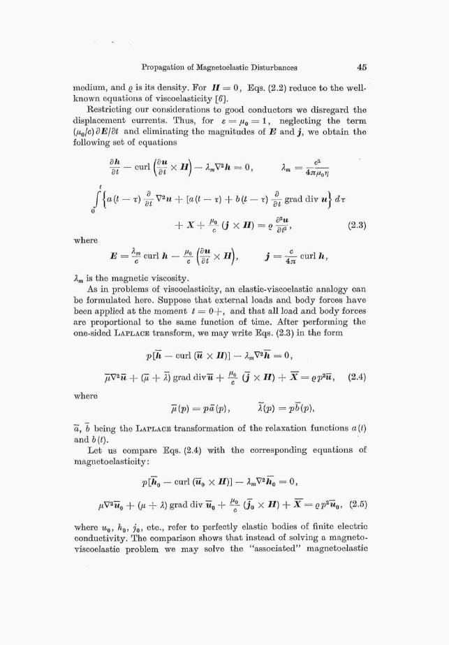
medium, and Q is its density. For II = 0, Eqs. (2.2) reduce to the well-known equations of viscoelasticity [6],

Restricting our considerations to good conductors we disregard thedisplacement currents. Thus, for e = ju0 = 1, neglecting the term(,MO/C) dEjdl and eliminating the magnitudes of E and j , we obtain thefollowing set of equations

?* - cul-l l& x H) - W*h = 0,

/I \a(t — T) -57 V2M -|- [a(t — T) -f- 6(t — T) -%? grad div 'J ( at ot

o

-1- X + &• (j X II) = o ~ , (2.3)

whereE = -^ curl / » - — h r r X f l , 1 — -i— curl /t,

c c \ oi / J 4JI

Xm is the magnetic viscosity.As in problems of viscoelasticity, an elastic-viscoelastic analogy can

be formulated here. Suppose that external loads and body forces havebeen applied at the moment t = 0+, and that all load and body forcesare proportional to the same function of time. After performing theone-sided LAPLACE transform, we may write Eqs. (2.3) in the form

- curl {u X II)] - l.mV2h = 0,

I) grad divw + * ( j x f l ) + I = QV2u, (2.4)

where

a, b being the LAPLACE transformation of the relaxation functions a (t)and b(t).

Let us compare Eqs. (2.4) with the corresponding equations ofmagnetoelasticity:

p[h0 - curl (u0 x II)] - AmV*h0 = 0,

|- (/i + A) grad div M0 + ^ (Jo X II) + X = ep*u0, (2.5)

where uQ, ha, j g , etc., refer to perfectly elastic bodies of finite electricconductivity. The comparison shows that instead of solving a magneto-viscoelastic problem we may solve the "associated" magnetoelastic

46 SYLWESTER KALISKI and WITOLD NOWACKI

problem. When its solution has been obtained, the LAM:E constants /<, Aare replaced by the quantities Jl, X, which are the functions of the para-meter p ; the inverse LAPLACE transform of u0 then furnishes the solutionof the magnetoviscoelastio problem. This analogy, however, is only validwhen the load and body forces as well as the displacements in the boun-dary conditions of the problem are proportional to the same functionof time.

3. Boundary Conditions

Let us now disrass the boundary conditions for two viscoelastic mediaof finite electric conductivity with a plane contact surface. Suppose thatthe vector of the initial magnetic field is arbitrarily oriented with respectto the plane of the contact. Taking into account the homogeneous initialconditions assumed in Section 2, we establish the boundary conditionsfor the Laplace transforms of the mechanical and electromagneticquantities.

Two types of boundary conditions will be considered:

(a) boundary conditions for two viscoelastic media in contact, and

(b) boundary conditions for a viscoelastic medium in contact witha vacuum.

In case (a) we obtain a set of twelve boundary conditions (see [7]).The indices (1) and (2) denote the two media, and n the unit vector-normal to the plane of contact. We have

ill1) = J7<2> ff11.1 4 - Tal — (T12.1 4 - T~m

[n x

[n x (ftw-fcro)] = 0 , (3.1 >where

B=B0+b=/n0{H+h). (3.2)

The system (3.1) contains the conditions of continuity of the transformsof the displacements, the conditions of the equality of the transformsof the sums of the mechanical stresses and the components of MAXWELL'S.

Propagation of Magnetoelastio Disturbances 47

tension tensor, and the conditions of continuity of the transforms ofthe normal inductions and tangential fields for the moving boundarysurface. The last two conditions are given in linearized form using anapproximation for the terms in vjc and without introducing two-sidedvalues of the tangent field IIt. If the quantities ,M(IV), a = 1.2 of themedia are approximately equal, then the term connected with themotion of the contact surface may be disregarded in (3.1). If, in theboundary conditions of the type (b), the medium characterized by sub-script 1 is the vacuum, we must set

^=E^ in (3.1).

4. Limit Passage to the Ideal Conductor

Lettering Xm —>0 in (2.3) and replacing the relaxation functions a (t),b (t) by the LAMB constants fi, X, we pass from a viscoelastic body withfinite electric conductivity to the perfectly elastic and perfectly con-ducting body. Eliminating the quantities E and h from (2.3), we thenobtain the following equations:

fiV2u + (X + fi) grad div u + ^- [curl curl (u x II)] X H

where

E = -•&'(•••=• X II), h = curl (u X H). (4.2)

For a perfectly conducting viscoelastic body, it is sufficient to assumethat Xm —.>• 0. We then obtain the equation of motion

i

fla(t ~r)~ V% + [a(t — T) + b{t — T)] ~ grad div u\ dro

+ ^ [curl curl (u x H)] X II + X = Q J£, (4.3)

the boundary conditions (4.2) remaining valid.Note that with ,« = 0 and dufdt^O Eq. (4.1) reduces to the

acoustic equation of an ideal fluid. Similarly, taking coefficients a(t),b(t) in (4.3) that correspond to VOIGT'S model with a = 0, we obtainthe acoustic equation of a viscous liquid.

Passing from a body with mechanical and magnetic viscosities toa body that is perfectly conductive and elastic, we must also make theappropriate transitions to the limit in the boundary conditions. Here,

48 SYLWESTER KALISKI and WITOLD NOWACKI

the manner in which the ratio of the magnetic and mechanical viscositiesin the liquid and in the solid tends to zero is essential. This concernsthe coefficients of viscosity when the initial field II is perpendicular tothe contact surface (see Section 5).

In the present section, we give the boundary conditions for the casewhen the vector of the initial magnetic field is parallel to the contactplane. We consider two basic types of contact

(a) The displacements of the media are continuous across the contactsurface. We then have the following boundary conditions:

where the quantities Tni are given by (3.2) and the quantities h{ by (4.2).The quantities Tik can be then expressed explicitly in terms of thedisplacements M;.

(b) In the contact plane there appears the ideal tangential slip. Theboundary conditions now take the form

-(1) i md) , ^(2) i /ri(2>ff33 ~T -* 33 — " 3 3 ~T •>• 33 >

=0) _"ni ~~

4 = 1,2.(4.5)

The second condition (4.5) can be replaced by the relation between thetangential components of the vectors h" (tx. = 1,2) and the stirfacecurrents [7].

Vo(t)

x-,

5. Passage to the Limit in Boundary Conditions for H = H 3

If the initial magnetic field is perpendicular to the contact surfacethen the boundary conditions assume one of two forms depending onhow the mechanical and magnetic viscosities tend to zero. These boun-

dary conditions will be discussed fora particular one-dimensional problemwith shear strains since these influ-ence the alternative forms of theboundary conditions.

Let us consider a rigid plate on thesurface of a viscoelastic semi-spacewith finite electric conductivity. Thisplate is set in motion in a tangential

direction, the initial conditions being assumed homogeneous (Fig. 1).The equations of motion (2.3), then contain the function a(t) and thedependent variables % (z, t) = u and \ (z, t) — h. The remaining

g. 1.

Propagation of Magnotoelastic Disturbances 49

quantities either are equal to zero or do not enter the problem. Thus,the system (2.3) takes the form

*h dh 8*u _A'" dz* 0T + n dtdz ~ U )

J a(' - T> W¥r dr + !u It = ew' H* = H-o

Neglecting the inertia term in the equations of motion, we treat theproblem as quasi-static This does not influence the physical conditionson the boundary. After performing the Laplace transform on Eqs. (5.1),the initial conditions being assumed homogeneous, and after solvingthese equations we obtain the following relations:

u — Moo = Cxer*z,

where

Making use of the boundary condition for z = 0,

« (0 ,p ) -« 0 .we obtain

v — Va, = {v0 — Voo)erxz, (5.4)

^ v0 — Voo) 6-««. (5.5)

Here, w = pu is the transform of the velocity.It follows from relations (5.4) and (5.5) that

Eq. (5.6) is essential for the discussion of possible combinations of boun-dary conditions when the mechanical and magnetic viscosities tend tozero. For a solid body with Ji =£ 0, when the magnetic viscosity Xm aswell as the parameters characterizing the mechanical viscosity tendsimultaneously to zero, condition (5.6) always yields

«„=$«,, (5.7)

4 Kolsky/Prager, Stress Waves

50 SYLWESTEB KALISKI and WITOLD NOWAOKI

that is the continuity of tangential velocities. For the Voigt model withJi = fi{l -\-pr), x = plp, where ft is the coefficient of viscosity, Eq. (5.6)takes the form

IT = J- {5'8)

It is apparent from (5.8) that in the limit we obtain relation (5.7) whenXm and x tend to zero in such a way that their ratio remains constant.

For the MAXWELL model, we have n = ^ , where r = fi/ju.Eq. (5.6) therefore furnishes

If the process is assumed, in the limit, to be stationary, (5.9) becomes

It is apparent that when ^m -> 0 while /? ^ 0, in the Hmit we obtainthe boundary condition (5.7). If f}—>0, then according to the threepossibilities

^° >°° ^s P11)where s is a constant, we obtain the following boundary conditions:

. (h0 — AM) (5.12)

respectively. The variant (S ->- 0 is physically artificial, because it impliesa vanishing time of relaxation, and consequently excludes elastic stresses.For' the stationary laminar flow of a viscous liquid, (5.8) yields

(5.13)

Here, ft' denotes the coefficient of viscosity of the liquid. For /S' —s- 0the liquid becomes ideal. Depending on the manner in which Am and /3'tend to zero [see (5.11)], we obtain three variants of the boundary con-ditions corresponding to the physically significant cases.

When two media, for instance a viscous liquid and a viscoelasticsolid are in contact, we obtain the following equations for the MAXWELL

Propagation of Magnetoelastic Disturbances 51

model (here the process may also he stationary)

(5.14)

The first of these equations concerns the solid with the viscosity jS, andthe second the viscous liquid with the viscosity /?''. It follows from theseequations that on the contact surface z = 0 of these media the variants(5.12) of the boundary conditions may occur.

We conclude that a condition of the type ha) = h(2) may obtain,provided the surface currents vanish in the transition from the visco-elastic to the perfect conductor. The disappearance of the surface cur-rents is identical with the disappearance of the tangential componentof the stress tensor. This case occurs for a •liquid, for ^'\Xm -> 0. I t alsoappears for the MAXWELL model for PjXm —• 0; this case, however, shouldbe regarded as unrealistic.

6. Example

The simple example that will now be discussed, illustrates the ex-treme alternatives of the boundary conditions. Consider two perfectlyconductive media: an ideal liquid and a perfectly elastic solid, andsuppose the initial magnetic field to be perpendicular to their plane ofcontact. Assume moreover that a tangential force, varying harmonicallywith time, acts in this plane. We consider the one-dimensional problemin the x, s plane.

The liquid in the negative half-space z < 0 is denoted by theindex (2) and the elastic solid in the half-space z > 0 by the index (1).The magnetic permeability of both media is assumed to be 1.

The equations of motion of the media take the form

h =#-£-• (6-2)In these equations, the symbols

u = M<2>, h = hW, a2 = %a\ = if2/(4^(?2)

should be iised for the liquid, and the symbols172 / ,

4—,

4*

52 SYLWESTEB KALISKI and WITOLD NOWACKI

for the elastic solid. According to the discussion in the preceding sectionwe consider two extreme variants of the boundary conditions correspond-ing to the transition to the limit in the liquid:

For the first boundary condition, we have the following relations for3 = 0:

For the second boundary condition we find for 2 = 0

or dz ' 8z '(6-4)

o'£=Peia{ or ^e 2 —:—=Peliai.

Settingu(z,t) =u*(z)eiat, (6.5)

we obtain

1 ? * ^ 2 ? V. /

where

Taking into account the boundary conditions (6.3), we obtain

P p—- ei(a>t-az) (2) fA

where

Zl = ^as^j 4.

For the boundary conditions (6.4) we find

P v

(6.8)

As is readily seen from (6.7) and (6.8), we have radiation of waves ofidentical displacement or velocity amplitudes in the first case and iden-

Propagation of Magnotoelastic Disturbances 53

tical amplitudes of the field h or the derivative of the displacement inthe second case. Thus, depending on the manner in. which the mechanicaland magnetic viscosities in the liquid tend to zero, we have obtaineddifferent solutions to the contact problem between a liquid and a solid.

The manner in which the viscosities tend to zero in the solid has noinfluence on the solution for all physically realistic cases.

References

\1~\ KULIKOVSKIJ, A. G., and G. A. LJTJBIMOV: Magnetohydrodynamics (in Russian),Moscow: Fizmatgiz, 1962.

[2] STBWAKTSON, K.: Fluid Mooh. 8, No. 1 (1960).[3] KALISKI, S.: Proo. Vibr. Probl. 3, No. 1 (1962).[4] KALISKI, S., and W. NOWACKI: Bull. Acad. Polon. Sciences 10, No. 4 (1962).[5] KALISKI, S., and J. PETYKIEWICZ: Proc. Vibr. Probl. 1, No. 4 (1959).[6] FRHUDBNTHAI,, A. M., and H. GISIRINOER: Encyclopedia of Physics, Vol. VI,

Berlin/Gottingen/Heidelberg: Springer 1958.[7] KALISKI, 8.: Problems of Contin-uum Mechanics, Soc. Ind. Appl. Math., Phil-

adelphia, 1961.