Amplification of Nonlinear Strain Waves in Solids - A.V.Porubov.pdf
227
February 11, 2004 20:10 WSPC/Book Trim Size for 9in x 6in ws-book9x6 Publishers’ page
-
Upload
kollesdestefa -
Category
Documents
-
view
22 -
download
1
Transcript of Amplification of Nonlinear Strain Waves in Solids - A.V.Porubov.pdf

February 11, 2004 20:10 WSPC/Book Trim Size for 9in x 6in ws-book9x6
Publishers’ page
i

February 11, 2004 20:10 WSPC/Book Trim Size for 9in x 6in ws-book9x6
Publishers’ page
ii

February 11, 2004 20:10 WSPC/Book Trim Size for 9in x 6in ws-book9x6
Publishers’ page
iii

February 11, 2004 20:10 WSPC/Book Trim Size for 9in x 6in ws-book9x6
Publishers’ page
iv
February 11, 2004 20:10 WSPC/Book Trim Size for 9in x 6in ws-book9x6
To my parents
v
February 11, 2004 20:10 WSPC/Book Trim Size for 9in x 6in ws-book9x6
vi

February 11, 2004 20:10 WSPC/Book Trim Size for 9in x 6in ws-book9x6
Preface
It is known that the balance between nonlinearity and dispersion may resultin an appearance of localized long bell-shaped strain waves of permanentform (solitary waves or solitons) which may propagate and transfer energyover the long distance along. Starting with the first documented watersurface solitary wave observation, made by J.Scott Russell yet in 1834,solitons in fluids were observed and generated many times. It was themost surprising fact, however, that despite of almost similar description ofstresses in fluids and solids, bulk longitudinal strain solitary waves have notbeen observed in nonlinearly elastic wave guides.
One of reason of the lack of the results on nonlinear wave in solids isthat the complete description of a three-dimensional (3-D) nonlinear con-tinuum is a difficult problem. That is why initial 3-D problems are usuallyreduced to the one-dimensional (1-D) form in order to clarify the simplestbut qualitatively new analytical solutions. Certainly the cylindrical elasticrod seems to be a suitable real-life 1-D wave guide. Recently, the theory hasbeen developed to account for long longitudinal strain solitary waves prop-agating in a free lateral surface elastic rod with permanent cross section.The nonlinearity, caused by both the finite stress values and elastic mate-rial properties, and the dispersion resulting from the finite transverse sizeof the rod, when in balance allow the propagation of the bulk strain soli-tary waves. Motivated by analytical theoretical predictions, there has beensuccessful experimental generation of strain solitary waves in a polystyrenefree lateral surface rod using the holographic interferometry. Hence it wasproven that bulk long localized nonlinear strain waves of permanent formreally exist.
However, presence of a dissipation (accumulation) destroys the balancebetween nonlinearity and dispersion, and nonlinear strain wave in the rod
vii
February 11, 2004 20:10 WSPC/Book Trim Size for 9in x 6in ws-book9x6
viii Book Title
may attenuate or amplify. One possibility occurs when the radius of therod varies. Dissipative (active) effects may be caused by internal featuresof the elastic material, hence, an irreversible part should be included intothe stress tensor in addition to the reversible one depending only upon thedensity of the Helmholtz energy. Dissipation (accumulation) may also comein an elastic wave guide through phenomena occurring at its lateral surface.Among the volume sources of dissipation/accumulation one can mention amicrostructure, point moving defects, thermal effects. When dissipationand activation act together there may be another balance resulted in a for-mation of a bell-shaped wave with the amplitude and the velocity prescribedby the condition of the dissipative/active balance. Hence the wave is se-lected. Note that there exist another kind of nonlinear wave of a permanentshape sustained either by a balance between nonlinearity and dissipation orby a balance between nonlinearity, dispersion and dissipation. This wavehas the form of a shock and is often called kink-shaped wave or simply kink.
The amplification of the waves (i.e., growth of the amplitude) may causethe appearance of plasticity zones or microcracks in a wave guide. This isof importance for an assessment of durability of elastic materials and struc-tures, methods of non-destructive testing, determination of the physicalproperties of elastic materials, particularly, polymeric solids, and ceramics.Bulk waves provide better suited detection requirements than surface strainwaves in setting up a valuable non-destructive test for pipelines.
Inclusion of dissipation (accumulation) yields nonlinear dispersive- dis-sipative governing equations that are nonintegrable as a rule. Hence, onlyparticular, usually travelling wave, solutions may be obtained analytically.Certainly, these solutions require specific initial conditions. Moreover, theyusually have no free parameters, and additional relationships between theequation coefficients are required for the existence of the solutions. That iswhy the obtaining of the exact solutions is often considered as useless bymany authors preferring to apply numerical methods only.
I would like to achieve two tasks in this monograph. First, it is plannedto provide the sequential analytical consideration of the strain waves am-plification/attenuation and selection in solids, mainly in an elastic rod. Itmay be of interest for those working in the field of solid mechanics. Anothertask is to demonstrate the use of even particular analytical solutions for thedescription of unsteady nonlinear wave processes. It may attract the atten-tion of the specialists in various fields since the structure of the governingequations is rather universal. The content is essentially based on the authorprevious research. However, many works were done in a collaboration. The

February 11, 2004 20:10 WSPC/Book Trim Size for 9in x 6in ws-book9x6
Chapter Title for Preface ix
author thanks a lot Profs. G.V. Dreiden, I.L. Kliakhandler, G.A. Maugin,F. Pastrone, D.F. Parker, A.M. Samsonov, M.G. Velarde; Mr. V.V. Gurskyand Mrs. I.V. Semenova for a long time fruitful collaboration. The bookpreparation has been supported by the INTAS grant 99-0167 and by theRFBR under Grant 2000-01-00482.
I dedicate this book to my parents. They always believe in my effortsand expected this book more than whoever it may be.
Saint-Petersburg, December, 2002 A.V. Porubov
February 11, 2004 20:10 WSPC/Book Trim Size for 9in x 6in ws-book9x6
x Book Title

February 11, 2004 20:10 WSPC/Book Trim Size for 9in x 6in ws-book9x6
Contents
Preface vii
1. Basic concepts 11.1 Single nonlinear waves of permanent shape . . . . . . . . . 2
1.1.1 Monotonic bell-shaped solitary waves . . . . . . . . . 21.1.2 Oscillatory bell-shaped solitary waves . . . . . . . . . 61.1.3 Kink-shaped waves . . . . . . . . . . . . . . . . . . . 91.1.4 Periodic nonlinear waves . . . . . . . . . . . . . . . . 12
1.2 Formation of nonlinear waves of permanent shape from anarbitrary input . . . . . . . . . . . . . . . . . . . . . . . . . 131.2.1 Bell-shaped solitary wave formation from an initial
localized pulse . . . . . . . . . . . . . . . . . . . . . . 151.2.2 Kink-shaped and periodic waves formation . . . . . . 26
1.3 Amplification, attenuation and selection of nonlinear waves 27
2. Mathematical tools for the governing equations analysis 312.1 Exact solutions . . . . . . . . . . . . . . . . . . . . . . . . . 31
2.1.1 Direct methods and elliptic functions . . . . . . . . . 312.1.2 Painleve analysis . . . . . . . . . . . . . . . . . . . . 352.1.3 Single travelling wave solutions . . . . . . . . . . . . 362.1.4 Exact solutions of more complicated form . . . . . . 42
2.2 Asymptotic solutions . . . . . . . . . . . . . . . . . . . . . . 472.3 Numerical methods . . . . . . . . . . . . . . . . . . . . . . . 51
2.3.1 Nonlinear evolution equations . . . . . . . . . . . . . 522.3.2 Nonlinear hyperbolic equations . . . . . . . . . . . . 57
2.4 Use of Mathematica . . . . . . . . . . . . . . . . . . . . . . 59
xi

February 11, 2004 20:10 WSPC/Book Trim Size for 9in x 6in ws-book9x6
xii Book Title
3. Strain solitary waves in an elastic rod 633.1 The sources of nonlinearities . . . . . . . . . . . . . . . . . . 643.2 Modelling of nonlinear strain waves in a free lateral surface
elastic rod . . . . . . . . . . . . . . . . . . . . . . . . . . . . 663.2.1 Statement of the problem . . . . . . . . . . . . . . . 663.2.2 Derivation of the governing equation . . . . . . . . . 69
3.3 Double-dispersive equation and its solitary wave solution . . 703.4 Observation of longitudinal strain solitary waves . . . . . . 753.5 Reflection of solitary wave from the edge of the rod . . . . . 79
4. Amplification of strain waves in absence of external en-ergy influx 874.1 Longitudinal strain solitary wave amplification in a narrow-
ing elastic rod . . . . . . . . . . . . . . . . . . . . . . . . . . 874.1.1 Governing equation for longitudinal strain waves
propagation . . . . . . . . . . . . . . . . . . . . . . . 874.1.2 Evolution of asymmetric strain solitary wave . . . . . 904.1.3 Experimental observation of the solitary wave ampli-
fication . . . . . . . . . . . . . . . . . . . . . . . . . . 934.2 Strain solitary waves in an elastic rod embedded in another
elastic external medium with sliding . . . . . . . . . . . . . 954.2.1 Formulation of the problem . . . . . . . . . . . . . . 964.2.2 External stresses on the rod lateral surface . . . . . . 994.2.3 Derivation of strain-displacement relationships inside
the rod . . . . . . . . . . . . . . . . . . . . . . . . . . 1004.2.4 Nonlinear evolution equation for longitudinal strain
waves along the rod and its solution . . . . . . . . . 1024.2.5 Influence of the external medium on the propagation
of the strain solitary wave along the rod . . . . . . . 1044.2.6 Numerical simulation of unsteady strain wave propa-
gation . . . . . . . . . . . . . . . . . . . . . . . . . . 1064.3 Strain solitary waves in an elastic rod with microstructure . 114
4.3.1 Modelling of non-dissipative elastic medium with mi-crostructure . . . . . . . . . . . . . . . . . . . . . . . 114
4.3.2 Nonlinear waves in a rod with pseudo-continuumCosserat microstructure . . . . . . . . . . . . . . . . 117
4.3.3 Nonlinear waves in a rod with Le Roux continuummicrostructure . . . . . . . . . . . . . . . . . . . . . . 120

February 11, 2004 20:10 WSPC/Book Trim Size for 9in x 6in ws-book9x6
Chapter Title for Front Matter xiii
4.3.4 Concluding remarks . . . . . . . . . . . . . . . . . . 121
5. Influence of dissipative (active) external medium 1235.1 Contact problems: various approaches . . . . . . . . . . . . 1235.2 Evolution of bell-shaped solitary waves in presence of ac-
tive/dissipative external medium . . . . . . . . . . . . . . . 1255.2.1 Formulation of the problem . . . . . . . . . . . . . . 1255.2.2 Dissipation modified double dispersive equation . . 1265.2.3 Exact solitary wave solutions of DMDDE . . . . . . 1285.2.4 Bell-shaped solitary wave amplification and selection 1305.2.5 Concluding remarks . . . . . . . . . . . . . . . . . . 134
5.3 Strain kinks in an elastic rod embedded in an ac-tive/dissipative medium . . . . . . . . . . . . . . . . . . . . 1365.3.1 Formulation of the problem . . . . . . . . . . . . . . 1375.3.2 Combined dissipative double-dispersive equation . . 1385.3.3 Exact solutions . . . . . . . . . . . . . . . . . . . . . 1415.3.4 Weakly dissipative (active) case . . . . . . . . . . . . 1435.3.5 Weakly dispersive case . . . . . . . . . . . . . . . . . 1455.3.6 Summary of results and outlook . . . . . . . . . . . . 150
5.4 Influence of external tangential stresses on strain solitarywaves evolution in a nonlinear elastic rod . . . . . . . . . . 1525.4.1 Formulation of the problem . . . . . . . . . . . . . . 1525.4.2 Derivation of the governing equation . . . . . . . . . 1535.4.3 Symmetric strain solitary waves . . . . . . . . . . . . 1555.4.4 Evolution of asymmetric solitary waves . . . . . . . . 159
6. Bulk active or dissipative sources of the amplification and selection1636.1 Nonlinear bell-shaped and kink-shaped strain waves in mi-
crostructured solids . . . . . . . . . . . . . . . . . . . . . . . 1646.1.1 Modelling of a microstructured medium with dissipa-
tion/accumulation . . . . . . . . . . . . . . . . . . . 1656.1.2 Bell-shaped solitary waves . . . . . . . . . . . . . . . 1696.1.3 Kink-shaped solitary waves . . . . . . . . . . . . . . 1726.1.4 Concluding remarks . . . . . . . . . . . . . . . . . . 176
6.2 Nonlinear seismic solitary waves selection . . . . . . . . . . 1786.2.1 Modelling of nonlinear seismic waves . . . . . . . . . 1786.2.2 Asymptotic solution of the governing equation . . . . 1806.2.3 Numerical simulations . . . . . . . . . . . . . . . . . 183
6.3 Moving defects induced by external energy flux . . . . . . . 188

February 11, 2004 20:10 WSPC/Book Trim Size for 9in x 6in ws-book9x6
xiv Book Title
6.3.1 Basic concepts and derivation of governing equations 1886.3.2 Nonlinear waves in a medium . . . . . . . . . . . . . 1906.3.3 Nonlinear waves in a plate . . . . . . . . . . . . . . . 192
6.4 Thermoelastic waves . . . . . . . . . . . . . . . . . . . . . . 1936.4.1 Nonlinear waves in thermoelastic medium . . . . . . 1956.4.2 Longitudinal waves in thermoelastic rod . . . . . . . 196
Bibliography 199
Index 211

February 11, 2004 20:10 WSPC/Book Trim Size for 9in x 6in ws-book9x6
Chapter 1
Basic concepts
This chapter is focused on some features of nonlinear waves to be usedfurther in the book. Linear waves are accounted for the linear equations,they have infinitesimal amplitude. Nonlinear waves are described by non-linear equations. In contrast to the linear waves, an amplitude, a veloc-ity and a wave number of the nonlinear waves are connected to one an-other. More general information about nonlinear waves may be found innumerous special books, like Ablowitz and Segur (1981); Bhatnagar (1979);Calogero and Degasperis (1982); Newell (1985); Sachdev (1987); Whitham(1974) etc.
The governing equations for the nonlinear strain waves to be consideredare nonitegrable by the inverse scattering transform method, and only par-ticular exact solutions may be obtained. Of special interest are the singletravelling wave solutions that keep their shapes on propagation. This is aresult of the balances between various factors affecting the wave behaviour.There are two main types of the nonlinear travelling solitary waves whichcould propagate keeping its shape, bell-shaped and kink-shaped solitarywaves. The bell-shaped solitary wave usually appears as a result of a bal-ance between nonlinearity and dispersion. The kink-shaped wave may besustained by different balances, one possibility occurs when nonlinearity isbalanced by dissipation (or accumulation) , another case corresponds to thesimultaneous balance between dispersion, nonlinearity and dissipation (oraccumulation). The single travelling wave solution requires specific initialconditions. However, one can show that these solutions account for thefinal quasistationary part of an arbitrary initial pulse evolution. This un-steady process may be described analytically for the integrable equationsor numerically for others. We illustrate all mentioned above further in thisChapter.
1

February 11, 2004 20:10 WSPC/Book Trim Size for 9in x 6in ws-book9x6
2 Amplification of Nonlinear Strain Waves in Solids
1.1 Single nonlinear waves of permanent shape
1.1.1 Monotonic bell-shaped solitary waves
The simplest celebrated model equation containing nonlinear and dispersiveterms is the well-known Korteweg- de Vries (KdV) equation Korteweg andde Vries (1895),
ut + 2b u ux + d uxxx = 0, (1.1)
whose exact one-parameter single solitary wave solution is
u = 6d
bk2 cosh−2 k(x− 4dk2t). (1.2)
The wave amplitude A = 6dk2/b and the velocity V = 4dk2 dependupon the wave number k which is a free parameter. One can call the solution(1.2) travelling solitary wave one since it depends upon the phase variableθ = x−V t only, and monotonic solitary wave since it decays monotonicallywhen |θ| → ∞. Typical shape of the wave is shown in Fig. 1.1 where onecan see also that the wave is symmetric with respect to its maximum.
-30 -20 -10 10 20 30x
0.2
0.4
0.6
0.8
u
Fig. 1.1 Monotonic solitary wave (solid line) and its first derivative (dashed line)
Sometimes there is a need for the inclusion of higher- order deriva-tive (dispersion) or nonlinear terms into Eq.(1.1). A particular case arisesfor water waves when surface tension suppresses coefficient d Hunter andScheurle (1988) and fifth-order dispersion u5x is added in Eq.(1.1).Also higher- order derivative terms model weak nonlocality Engelbrecht
February 11, 2004 20:10 WSPC/Book Trim Size for 9in x 6in ws-book9x6
Basic concepts 3
and Braun (1998), provide an improvement of bad dispersive propertiesChristov et. al (1996); Maugin and Muschik (1994), account for a contin-uum limit of discrete models with far neighbour interactions Kosevich andSavotchenko (1999), to say nothing of dissipative (active) generalizations.An example of the inclusion of higher- order nonlinearity is the Sawada-Kotera equation Sawada and Kotera (1974).
Hence, the following nonlinear equation may be considered:
ut + 2b u ux + 3c u2ux + r u uxxx + s ux uxx + d u3x + f u5x = 0, (1.3)
We get from Eq.(1.3) a fifth-order (in space derivatives) KdV equationHunter and Scheurle (1988) when c = r = s = 0. This equation was studiedin many papers, see, e.g., Karpman (1993); Karpman (1998); Karpman andVanden-Broeck (1995); Kawahara (1972); Kawahara and Takaoka (1988);Benilov et. al (1993); Grimshaw et. al (1994). When, in addition d = 0,the resulting equation models the LC ladder electrical transmittion lines.Its solutions were obtained in Nagashima and Kuwahara (1981); Kano andNakayama (1981). A special integrable case corresponds to the Sawada-Kotera equation with b = d = 0, c = −r = −s/2 = 10, f = 1 Sawadaand Kotera (1974). Its solitary wave solutions may be found in Parkes andDuffy (1996), see also references therein.
Equation (1.3) is obviously nonintegrable by the Inverse ScatteringTransform method, and only particular exact solutions may be obtained.Let us consider an exact solution vanishing at infinity. In case of the fifth-order KdV equation it has the form Kano and Nakayama (1981):
u =210d
13bk2 cosh−4 k(x− V t), (1.4)
with k2 = −d/(52f). Hence the width of the wave is prescribed by thedispersion coefficients d and f which should be of opposite sign. For thewave velocity we have V = 144dk2/13 = −36d2/(169f). Hence, simultane-ous triggering of the signs of b, d and f results in changing only the wavepropagation direction.
In the general case the exact solitary- wave solution has a form similarto the KdV soliton (1.2),
u = A cosh−2 k(x− V t). (1.5)
Important particular cases are:

February 11, 2004 20:10 WSPC/Book Trim Size for 9in x 6in ws-book9x6
4 Amplification of Nonlinear Strain Waves in Solids
(i) In presence of only cubic nonlinear term, r = s = 0, we get the solutionwith fixed parameters,
A = 2
√−30f
ck2, V = 4k2(2b
√−30f
c−5d−116f k2), k2 =
b√−30f/c− 3d
60f.
(1.6)In this case the existence of solution vanishing at infinity is provided by
the linear fifth order term f u5x. Indeed at f = 0 we get from Eq.(1.3) theGardner equation whose solution is Grimshaw et. al (1999):
u =A1
coshm(x− V t) + B1, (1.7)
where
A1 =3√
2d m2
√2b2 + 9cdm2
, B1 =√
2b√2b2 + 9cdm2
, V = dm2. (1.8)
An important feature of the solution is the existence of the finite limitingamplitude when B is large Slyunyaev and Pelinovsky (1999). However, atnonzero f a substitution of Eq.(1.7) into Eq.(1.3) yields B1 = 1, cosh m(x−V t) + 1 = 2 cosh2 m(x − V t)/2, and we get the solution (1.5), (1.6) withm = 2k.(ii) When only quadratic higher- order term r uuxxx is taken into account,c = s = 0, the fixed parameters of the solution (1.5) are
A =30fk2
r, V =
2(50b2f2 + 5bdfr − 3d2r2)25f r2
, k2 =5bf − dr
10fr. (1.9)
Note that the solution exists at d = 0.(iii) In case c = r = 0 the parameter k is free but an additional restrictionon the equation coefficients holds,
A =60fk2
s, V = 4k2(d + 4f k2), 10b f = d s. (1.10)
One can see that s may be excluded from the amplitude expression usingthe third formula from (1.10). Then the amplitude coincides with that ofthe KdV soliton (1.2). We also see that the wave velocity consists of twoparts, V1 = 4dk2 and V2 = 16fk4, the first of which being exactly the KdVsoliton velocity. Let us rewrite the ODE reduction of the equation (1.3) inthe form ( ′ = ∂/∂θ, θ = x− V t):
b u2 + d u′′ − V1u +s
2u′2 + f u′′′′ − V2 u = 0.

February 11, 2004 20:10 WSPC/Book Trim Size for 9in x 6in ws-book9x6
Basic concepts 5
One can check that the solution (1.5), (1.10) satisfies separately
b u2 + d u′′ − V1u = 0, (1.11)s
2u′2 + f u′′′′ − V2 u = 0,
where the first of these equations is the ODE reduction of the KdV equation(1.1) having a one-parameter solitary- wave solution.(iv) Higher order nonlinear terms may support the existence of solitary-wave solutions even in absence of the linear dispersion terms. Higher- ordernonlinear terms provide bounded localized solutions at d = 0 in contrast tothe case c = r = s = d = 0 Kano and Nakayama (1981). The parametersof the solution (1.5) are
A =120fk4
b + 2k2(r + s), V = 16fk4,
while k satisfies the equation
4[30cf − r(r + s)]k4 + 2bsk2 + b2 = 0.
Thanks to the higher order terms the solitary- wave solution may existeven in the absence of the KdV’s nonlinear term, b = 0, provided that therestriction 30cf−r(r+s) = 0 is satisfied. Then k may be a free parameter.
When f = 0 we have
A =3cd− 2b(2r + s)
c(r + s), V =
2d[3cd− 2b(2r + s)](r + s)(2r + s)
, k2 =3cd− 2b(2r + s)2(r + s)(2r + s)
.
There is no exact solution vanishing at infinity in the case d = f = 0.Instead the solution in the form of a solitary wave on an ”pedestal” maybe obtained as
u = A cosh−2 k(x− V t) + B, (1.12)
with
A =2k2(2r + s)
c,B = − (2r + s)[b + 2k2(r + s)]
3c(r + s),
V =s(2r + s)[4k4(r + s)2 − b2]
3c(r + s)2.
Even equations with dissipation may possess bell-shaped solitary wavesolution. In particular, it was recently found Garazo and Velarde (1991);

February 11, 2004 20:10 WSPC/Book Trim Size for 9in x 6in ws-book9x6
6 Amplification of Nonlinear Strain Waves in Solids
Rednikov et. al (1995) that appropriately heating a shallow horizontal liq-uid layer long free surface waves u(x, t) can be excited whose evolution isgoverned by a dissipation-modified Korteweg- de Vries (DMKdV) equation
ut + 2α1 uux+∼α2 uxx + α3 uxxx+
∼α4 uxxxx+
∼α5 (uux)x = 0. (1.13)
The coefficients in Eq.(1.13) depend upon parameters characterizing theliquid (Prandtl number etc.), temperature gradient across the layer, and itsdepth. The exact travelling bell-shaped solitary wave solution have beenobtained in the form (1.12) Lou et. al (1991); Porubov (1993) with
A = 12∼α4 k2/
∼α5, B = −(
∼α2 +4
∼α4 k2)/
∼α5,
V = −2α1∼α2 /
∼α5, α3 = 2α1
∼α4 /
∼α5 . (1.14)
The meaning of the last expression in (1.14) is similar to that in case c =r = 0 for Eq.(1.3). Indeed, when the relationships for V and α3 hold, theODE reduction Eq.(1.13) may be rewritten as
(∼α2
∂
∂θ+
2α1∼α2
∼α5
)
(uθ +
∼α4∼α2
uθθθ +∼α5
2∼α2
(u2)θ
)= 0, (1.15)
The restrictions on the equation coefficients do not necessary providean evidence of the KdV ODE reduction like Eqs.(1.11), (1.15). Particularcase corresponds to the Kawahara equation (Eq.(1.13) with
∼α5= 0) whose
exact solution is Kudryashov (1988):
u =15α3
3
128α1∼α
2
4
cosh−2(α3
8∼α4
θ)(1− tanh(α3
8∼α4
θ)), (1.16)
where V = 5α33,
∼α2= α2
3/(16∼α4).
All solutions (1.4), (1.5), (1.7) account for monotonic and symmetricsolitary waves. Despite difference in their functional form they have one andthe same shape shown in Fig. 1.1. In contrast to them exact solitary wavesolution (1.16) of the Kawahara equation is monotonic but asymmetric, seeFig. 1.2.
1.1.2 Oscillatory bell-shaped solitary waves
The solitary wave does not decay necessarily in a monotonic manner. ThusKawahara (1972) studied decay at infinity of the wave solution of the fifth-

February 11, 2004 20:10 WSPC/Book Trim Size for 9in x 6in ws-book9x6
Basic concepts 7
-30 -20 -10 10 20 30x
-0.1
-0.05
0.05
u b
-30 -20 -10 10 20 30x
0.2
0.4
0.6
0.8
u a
Fig. 1.2 Symmetric (solid line) vs asymmetric monotonic solitary wave (dashed line).a) profiles; b)their first derivatives.
order KdV equation using linearized equation analysis phase analysis. Itwas found that the wave decays monotonically or oscillatory dependingupon the parameter ε, which is proportional (in our notations) to d andis inverse proportional by the product of f and the wave velocity. Thesame technique has been used in Karpman (2001) when nonlinear term inthe fifth-order KdV equation is of the form up ux. The oscillatory solitary-wave solution is shown in Fig. 1.3. The profile of the first derivative withrespect to the phase variable reveals its symmetric nature.
Eq.(1.3) does not possess exact oscillatory solitary wave solution. How-

February 11, 2004 20:10 WSPC/Book Trim Size for 9in x 6in ws-book9x6
8 Amplification of Nonlinear Strain Waves in Solids
-4 -2 2 4x
-0.5
-0.25
0.25
0.5
0.75
1
u
Fig. 1.3 Oscillatory solitary wave (solid line) and its first derivative (dashed line)
ever, it may be described asymptotically. Certainly the fifth-order KdVequation is often considered as a perturbed KdV equation. First the asymp-totic solution is obtained which consists of the KdV solitary wave solutionand a small perturbation that oscillates but does not vanish at infinityor a non-local solution Benilov et. al (1993); Hunter and Scheurle (1988);Karpman (1993); Karpman (1998). Let us consider the fifth- order deriva-tive term and higher- order nonlinear terms as small perturbations assum-ing f = δF , r = δR, s = δS, c = δC, δ << 1. The asymptotic solutionu = u(θ), θ = x− V t, is sought in the form
u = u0(θ) + δ u1(θ) + ..., (1.17)
with ui → 0 at |θ| → ∞. In the leading order we get the KdV equation(1.1) for the function u0 whose travelling solitary wave solution is (1.2). Inthe next order an inhomogeneous linear equation results for u1,
2b (u0u1)θ + d u1,θθθ − 4dk2 u1,θ = −F u0,θθθθθ − 3C u20u0,θ −R u0u0,θθθ−
S u0,θu0,θθ. (1.18)
Its solution vanishing at infinity is
u1 = (3C
4b+
5bF
2d2− 2R + S
4d) u2
0+(S
b+
4R
b− 14F
d− 9Cd
b2)k2 u0− 2k2F
dθ u0,θ.
(1.19)

February 11, 2004 20:10 WSPC/Book Trim Size for 9in x 6in ws-book9x6
Basic concepts 9
The shape of the solution u = u0(θ) + δ u1(θ) depends upon the valuesof the coefficients of Eq.(1.3). It may account for an oscillatory solitarywave solution first obtained numerically in Kawahara (1972), see Fig. 1.3.In the case of the fifth-order KdV equation, this profile exists at positive d
and f , what corresponds to the Case IV in Kawahara (1972).Finally, there exist nonlinear equations having exact travelling wave
solutions in the form of an oscillatory solitary wave. In particular, anequation
ut + a ux + 2b u ux + 3c u2ux + d u3x + f u5x + g u7x = 0, (1.20)
possesses the exact solution
u =
√35g
ck3 cosh−1 k(x− V t)
(24 cosh−2 k(x− V t)− 288
17
),
where b = 0, k2 = 17f/(581g), V = a + 102825k6g/289. The equationcoefficients should be connected by d g = 37.405 f2.
Oscillatory solitary waves of permanent shape arise also in dissipativeproblems, however, usually they are asymmetric and may be found onlynumerically.
1.1.3 Kink-shaped waves
The celebrated Burgers’ equation Burgers (1948) is the simplest equationthat models the balance between nonlinearity and dissipation,
ut + 2b u ux + g uxx = 0, (1.21)
In particular, it possesses the exact travelling solution of permanent form,
u = Am tanh(mθ) + B, (1.22)
where
A =g
b, B =
V
2b, m− free.
If the boundary conditions are
u → h1 at θ →∞, u → h2 at θ → −∞, (1.23)

February 11, 2004 20:10 WSPC/Book Trim Size for 9in x 6in ws-book9x6
10 Amplification of Nonlinear Strain Waves in Solids
then
m =(h1 − h2)b
2g, V = b(h1 + h2).
-4 -2 2 4x
-1
1
2
3
4
5
u
Fig. 1.4 Burgers’ kink-shaped wave
The shape of the solution (1.22), called kink, is shown in Fig. 1.4. Kinksmay arise also due to the balance between nonlinearity, dispersion and dissi-pation like in the case of the Korteweg-de Vries-Burgers equation (KdVB),
ut + 2b u ux + g uxx + duxxx = 0, (1.24)
whose exact solution was obtained independently by many authors Vlieg-Hultsman and Halford (1991)
u = A tanh(mθ)sech2(mθ) + 2A tanh(mθ) + C, (1.25)
with
A =6g2
50V d, C =
V
2b, m =
g
10d.
It follows from the boundary conditions (1.23) that
h+ − h− = 2B, V = b(h+ + h−),
February 11, 2004 20:10 WSPC/Book Trim Size for 9in x 6in ws-book9x6
Basic concepts 11
and the solution exists under
h2+ − h2
− =12g2
25bd.
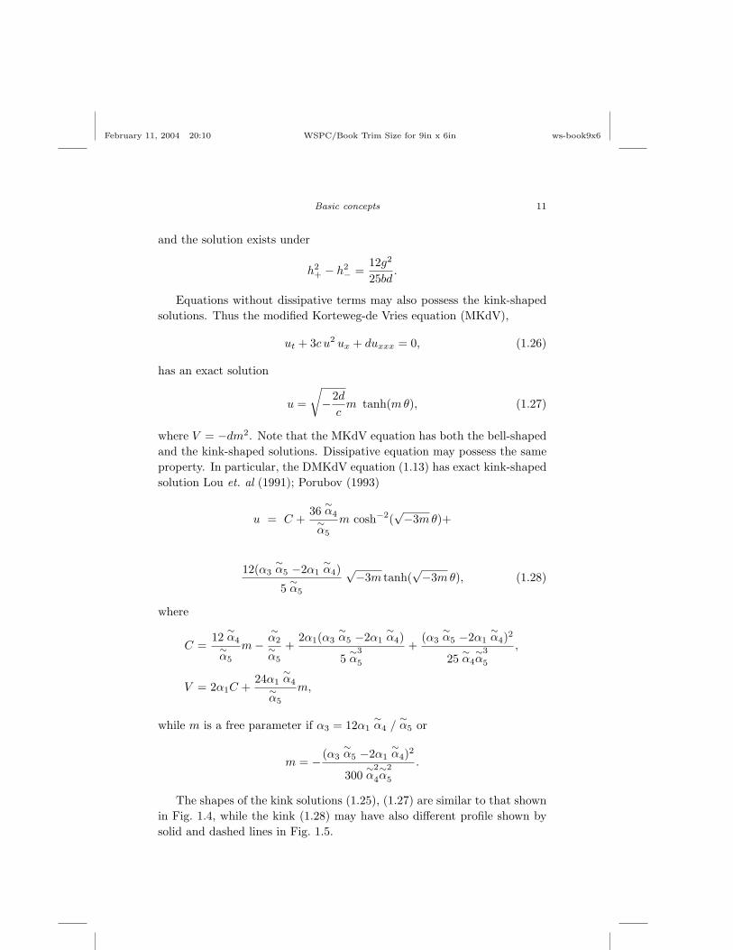
Equations without dissipative terms may also possess the kink-shapedsolutions. Thus the modified Korteweg-de Vries equation (MKdV),
ut + 3c u2 ux + duxxx = 0, (1.26)
has an exact solution
u =
√−2d
cm tanh(mθ), (1.27)
where V = −dm2. Note that the MKdV equation has both the bell-shapedand the kink-shaped solutions. Dissipative equation may possess the sameproperty. In particular, the DMKdV equation (1.13) has exact kink-shapedsolution Lou et. al (1991); Porubov (1993)
u = C +36
∼α4
∼α5
m cosh−2(√−3mθ)+
12(α3∼α5 −2α1
∼α4)
5∼α5
√−3m tanh(√−3mθ), (1.28)
where
C =12
∼α4
∼α5
m−∼α2∼α5
+2α1(α3
∼α5 −2α1
∼α4)
5∼α
3
5
+(α3
∼α5 −2α1
∼α4)2
25∼α4∼α
3
5
,
V = 2α1C +24α1
∼α4
∼α5
m,
while m is a free parameter if α3 = 12α1∼α4 /
∼α5 or
m = − (α3∼α5 −2α1
∼α4)2
300∼α
2
4
∼α
2
5
.
The shapes of the kink solutions (1.25), (1.27) are similar to that shownin Fig. 1.4, while the kink (1.28) may have also different profile shown bysolid and dashed lines in Fig. 1.5.

February 11, 2004 20:10 WSPC/Book Trim Size for 9in x 6in ws-book9x6
12 Amplification of Nonlinear Strain Waves in Solids
-4 -2 2 4x
-1.5
-1
-0.5
0.5
1
u
Fig. 1.5 Kink-shaped waves with a ”hat”
1.1.4 Periodic nonlinear waves
Usually single bell-shaped solitary wave solutions are the particular cases ofmore general periodic solutions. Thus Korteweg and de Vries (1895) foundthe periodic solution of the KdV equation (1.1),
u = 6d
bk2
(1− κ2 +
E
K+ κ2cn2(kθ, κ)
)(1.29)
where K and E are the complete elliptic integrals of the first and thesecond kind respectively , κ is the modulus of the Jacobian elliptic functionBateman and Erdelyi (1953-54); Byrd and Friedman (1954); Newille (1951).They called Eq.(1.29) the cnoidal wave solution since it is expressed throughthe Jacobi elliptic function cn . Cnoidal wave is not a linear superposition ofthe bell-shaped solitary waves. It tends to the single solitary wave solution(1.2) at κ → 1 as shown in the right column in Fig. 1.6 1. Exact periodicand bell-shaped solitary wave solutions correspond in the same mannerin case of the generalized 5th-order KdV equation (1.3) and the DMKdVequation (1.13).
Although many equations, like Burgers’, BKdV and DMKdV equationshave not exact bounded periodic solutions that transform into the kink-shaped ones, there exist exceptions. Thus the MKdV periodic solution
1Reprinted with permission from Elsevier Science

February 11, 2004 20:10 WSPC/Book Trim Size for 9in x 6in ws-book9x6
Basic concepts 13
Ablowitz and Segur (1981)
u =
√−2d
cmsn(mθ, κ), (1.30)
transforms into the kink solution (1.27) at κ → 1. Another example is adissipative nonlinear equation
ut + 2bu ux + 3c u2 ux + duxxx + f(u2)xx + guxx = 0, (1.31)
This evolution equation represents an analog of the hyperbolic equationto be derived further in Sec. 5.3. Its bounded periodic solution Porubov(1996) is
u =m√−c
cn(mθ, κ) sn(mθ, κ) dn(mθ, κ)C1 + cn2(mθ, κ)
− b
3c. (1.32)
with
C1 =1− 2κ2 +
√κ4 − κ2 + 1
3κ2, m2 =
3g2 − V
4√
κ4 − κ2 + 1,
and the following restrictions on the coefficients:
f = −12√−c, b = 3g
√−c.
The periodic wave solution (1.32) has a functional form different from boththe KdV cnoidal wave and the MKdV bounded periodic solution. Whenκ = 1 we have C1 = 0, and the solution (1.31) tends to the kink-shapedsolution (1.27) as it is shown in the left column in Fig. 1.6 in comparisonwith the transformation of the KdV cnoidal wave solution to the bell-shapedsolitary wave.
1.2 Formation of nonlinear waves of permanent shape froman arbitrary input
All solutions presented in previous section require specific initial conditions.In practice more important is to know how an arbitrary finite amplitudeinput evolves. Analytical solutions of unsteady problems may be obtainedif governing nonlinear equations are integrable Ablowitz and Segur (1981);Bhatnagar (1979); Calogero and Degasperis (1982); Dodd et. al (1982);Newell (1985), otherwise only numerical solutions are available. Often ini-tial input transforms into the stable quasistationary wave structures of

February 11, 2004 20:10 WSPC/Book Trim Size for 9in x 6in ws-book9x6
14 Amplification of Nonlinear Strain Waves in Solids
d
-10 -5 5 10x
-2
-1
1
2u
-10 -5 5 10x
-1
1
2
3u
c
-10 -5 5 10x
-2
-1
1
2u
-10 -5 5 10x
-1
1
2
3u
b
-10 -5 5 10x
-2
-1
1
2u
-10 -5 5 10x
-1
1
2
3u
a
-10 -5 5 10x
-0.4
-0.2
0.2
0.4u
-10 -5 5 10x
-0.4
-0.2
0.2
0.4u
Fig. 1.6 Comparison of the periodic solution (1.32) (left column) and the KdV cnoidalwave (1.29)(right column) for different values of the Jacobi modulus: (a)κ2 = 0.25, (b)κ2 = 0.995, (c)κ2 = 0.99995, (d)κ2 = 1. After Porubov and Velarde (2002).
permanent form which may be described by the analytical solutions. Alsothe analysis gives the conditions when the formation of them is possible.In this section we illustrate it using some instructive examples.

February 11, 2004 20:10 WSPC/Book Trim Size for 9in x 6in ws-book9x6
Basic concepts 15
1.2.1 Bell-shaped solitary wave formation from an initial
localized pulse
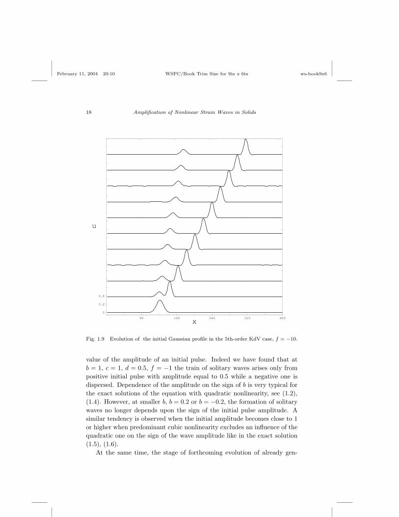
The fifth-order KdV was extensively studied numerically. The oscil-latory travelling solitary- wave solutions were found in Boyd (1991);Nagashima and Kuwahara (1981). The evolution of the initial monotonicsolitary wave into radiating or oscillatory solitary waves was simulated inBenilov et. al (1993); Karpman and Vanden-Broeck (1995). In a series ofpapers Salupere et. al (1997); Salupere et. al (2001) the solitary wave forma-tion from a periodic input was studied for an equation similar to Eq.(1.3).We shall study the evolution of a localized initial pulse. Previously, local-ized pulse evolution into an oscillatory solitary wave was considered inNagashima and Kuwahara (1981) for the equation ut + uux − γ2 u5x = 0.Below we consider the formation of solitary waves in the systems governedby Eq.(1.3). Following Porubov et. al (2002) we use two methods for com-putations, finite-difference and pseudo-spectral, see Sec. 2.3.2. Below onlythose results are shown that were obtained using both numerical methods.We have tried various shapes of the initial localized pulses, rectangular,Gaussian distribution etc.Influence of the fifth-order dispersive term. First the 5th-order KdVequation was studied. Since the role of the fifth-order derivative term is ofinterest the coefficients b and d in Eq.(1.3) were fixed for all computations,b = 1, d = 0.5. We found that the rectangular initial pulse splits into asequence of solitary waves when the coefficients of dispersive terms, d andf , are of opposite sign. For both coefficients positive the initial rectan-gular profile is dispersed without formation of any localized waves. Thedependence upon the sign of the ratio d/f is in agreement with the exactsolitary- wave solution (1.4) and the analysis of the dispersion relationKarpman (1993). However, more smooth Gaussian initial profiles providethe appearance of solitary waves even for positive coefficients when f israther small, e.g., f = 0.01.
The next result we have obtained is the dependence of the number ofsolitary waves upon the value of f when d/f < 0.
Shown in Fig. 1.7 is the formation of the train of solitary waves from aGaussian initial pulse in the KdV case, f = 0.
Figs. 1.8-1.10 demonstrate the decrease of the solitary waves for f =−1,−10,−50 respectively. Both the amplitude and the velocity decreasewith the increase of the absolute value of f in qualitative agreement withthe exact solution (1.4).The ratio between the amplitude and the velocity

February 11, 2004 20:10 WSPC/Book Trim Size for 9in x 6in ws-book9x6
16 Amplification of Nonlinear Strain Waves in Solids
40 80 120 160 200
x
0
0.2
0.4
u
Fig. 1.7 Evolution of the initial Gaussian profile in the KdV case, f = 0.
of each solitary wave in Fig. 1.7 is equal to 1.5 just as for the KdV soliton(1.2) . This ratio (and the amplitude) decreases with the decrease of f , from1.43 at f = −1 to 1.33 at f = −50. A similar tendency is revealed by thephase analysis of single travelling wave solutions, cf. Fig. 2 in Kawahara(1972). The ratio for the 5th- order KdV exact solution (1.4) is 1.46, theamplitude and the velocity for given b and d are −105/(1352f), −9/(169f),respectively. Only at small f = −0.1÷−0.15 are the numerical results forthe leading solitary wave in quantitative agreement with the exact solution(1.4). More important is that the decrease of f affects the solitary- wavetransformation from monotonic KdV solitons (1.2) to the oscillatory soli-tary waves. For convenience the last stages from Figs. 1.7-1.10 are collectedin Fig. 1.11. In case f = −1, Fig. 1.11(B), the higher leading solitary wave

February 11, 2004 20:10 WSPC/Book Trim Size for 9in x 6in ws-book9x6
Basic concepts 17
60 120 180 240 300
x
0
0.2
0.4
u
Fig. 1.8 Evolution of the initial Gaussian profile in the 5th-order KdV case, f = −1.
is oscillatory while other solitary waves remain monotonic, then the trans-formation occurs also for the second solitary wave, Fig. 1.11(C) . Alternatetransformation of the solitary waves confirms the dependence of the kindof solitary wave upon the value of the product of f and the wave amplitude(hence, its velocity) found in Kawahara (1972).
Finally, we have found that simultaneous triggering of the signs of b, d,f doesn’t affect the shapes of the solitary waves. They simply evolve to theopposite direction according to the analysis of the exact solution (1.4).Influence of the cubic nonlinearity. Now we add cubic nonlinearity,c 6= 0, while r = s = 0. The analytical solutions predict an action ofthe cubic nonlinear term depends upon the sign of c. Also the solution issensitive to the ratio between nonlinear terms contributions, b/c, and the
February 11, 2004 20:10 WSPC/Book Trim Size for 9in x 6in ws-book9x6
18 Amplification of Nonlinear Strain Waves in Solids
80 160 240 320 400
x
0
0.2
0.4
u
Fig. 1.9 Evolution of the initial Gaussian profile in the 5th-order KdV case, f = −10.
value of the amplitude of an initial pulse. Indeed we have found that atb = 1, c = 1, d = 0.5, f = −1 the train of solitary waves arises only frompositive initial pulse with amplitude equal to 0.5 while a negative one isdispersed. Dependence of the amplitude on the sign of b is very typical forthe exact solutions of the equation with quadratic nonlinearity, see (1.2),(1.4). However, at smaller b, b = 0.2 or b = −0.2, the formation of solitarywaves no longer depends upon the sign of the initial pulse amplitude. Asimilar tendency is observed when the initial amplitude becomes close to 1or higher when predominant cubic nonlinearity excludes an influence of thequadratic one on the sign of the wave amplitude like in the exact solution(1.5), (1.6).
At the same time, the stage of forthcoming evolution of already gen-

February 11, 2004 20:10 WSPC/Book Trim Size for 9in x 6in ws-book9x6
Basic concepts 19
100 200 300 400 500
x
0
0.2
0.4
u
Fig. 1.10 Evolution of the initial Gaussian profile in the 5th-order KdV case, f = −50.
erated solitary waves is not so sensitive to the value of b, while other an-alytical restrictions on the coefficients become more important. Besidesthe condition d/f < 0 following from the linear analysis Karpman (1993);Kawahara (1972), there is f/c < 0 resulted from the nonlinear exact so-lution (1.5), (1.6). Moreover, at small f one can anticipate an evidence ofthe condition d/c > 0 given by Eq.(1.8).
When c > 0, f < 0 all above mentioned inequalities are satisfied. Thenumber of solitary waves generated from the initial localized pulse increaseswith the increase of the value of c and fixed values of d = 0.5, f = −1 andalso b = 1 or b = 0.2. The velocity of the waves increases also, the width(proportional to 1/k) decreases, while the amplitude remains practically oneand the same. We also observed the alternate transformation of the solitary

February 11, 2004 20:10 WSPC/Book Trim Size for 9in x 6in ws-book9x6
20 Amplification of Nonlinear Strain Waves in Solids
140 180 220 260 300 340x
0
0.05
0.1
0.15
0.2
u
C
160 210 260 310 360 410x
0
0.1
0.2
0.3
0.4
u
D
70 90 110 130 150 170
x
0
0.05
0.1
0.15
0.2
u
A
100 130 160 190 220 250
x
0
0.02
0.04
0.06
0.08
0.1
u
B
Fig. 1.11 Transformation of the kind of solitary waves in the 5th-order KdV case. (A)f = 0, (B) f = −1, (C) f = −10, (D) f = −50.
waves from monotonic to oscillatory when c increases for both values of b.Independence of the amplitude of c doesn’t follow from the exact solution(1.6) as well as from the asymptotic solution. The third formula in (1.6)predicts growth of positive values of k2 only for b = 0.2 giving negativevalues for b = 1. However, let us express k through the amplitude A andsubstitute it into the expression for the velocity V . Then one can exhibit forboth values of b the similarity of the variation of the velocity with respectto c with that obtained in numerics.
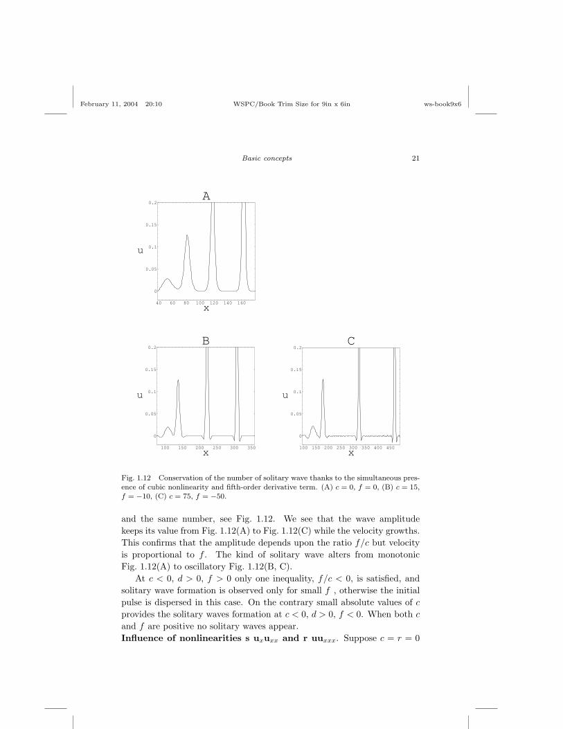
As found in previous subsection, the decrease of the negative f valuesaffects the decrease in the number of solitary waves. Assume b = 1, d = 0.5,we have tried simultaneous variations of c and f in order to sustain one
February 11, 2004 20:10 WSPC/Book Trim Size for 9in x 6in ws-book9x6
Basic concepts 21
100 150 200 250 300 350x
0
0.05
0.1
0.15
0.2
u
B
100 150 200 250 300 350 400 450x
0
0.05
0.1
0.15
0.2
u
C
40 60 80 100 120 140 160
x
0
0.05
0.1
0.15
0.2
u
A
Fig. 1.12 Conservation of the number of solitary wave thanks to the simultaneous pres-ence of cubic nonlinearity and fifth-order derivative term. (A) c = 0, f = 0, (B) c = 15,f = −10, (C) c = 75, f = −50.
and the same number, see Fig. 1.12. We see that the wave amplitudekeeps its value from Fig. 1.12(A) to Fig. 1.12(C) while the velocity growths.This confirms that the amplitude depends upon the ratio f/c but velocityis proportional to f . The kind of solitary wave alters from monotonicFig. 1.12(A) to oscillatory Fig. 1.12(B, C).
At c < 0, d > 0, f > 0 only one inequality, f/c < 0, is satisfied, andsolitary wave formation is observed only for small f , otherwise the initialpulse is dispersed in this case. On the contrary small absolute values of c
provides the solitary waves formation at c < 0, d > 0, f < 0. When both c
and f are positive no solitary waves appear.Influence of nonlinearities s uxuxx and r uuxxx. Suppose c = r = 0

February 11, 2004 20:10 WSPC/Book Trim Size for 9in x 6in ws-book9x6
22 Amplification of Nonlinear Strain Waves in Solids
80 100 120 140 160x
0
0.1
0.2
0.3
0.4
0.5
0.6
u
r=-1.60
80 100 120 140 160
x
0
0.1
0.2
0.3
0.4
0.5
0.6
u
r=-1.50
80 100 120 140 160
x
0
0.1
0.2
0.3
0.4
0.5
0.6
u
r=-1.57
Fig. 1.13 Equalization of the first and the second solitary waves and subsequent ex-ceeding of the second wave due to the alteration of the negative values of the coefficientr.
and vary s at fixed b, d and f , that we choose b = 1, d = 0.5, f = −1 . Itis found that the amount of solitary waves and its transition from mono-tonic to oscillatory don’t depend upon the value of s. The wave amplitudedecreases with the increase of s while the velocity keeps its value. Wavebehavior is not sensitive to the sign of s. The condition for the solitarywave formation d/f < 0 remains valid.
The fact the velocity doesn’t depend upon s is in agreement with theexact solution. Certainly, solitary waves exist outside the restriction from(1.10). We also used numerical values of the amplitude to define k andthen V using (1.10). A comparison of the velocities with those obtainednumerically demonstrates the more agreement the less is the value of b.

February 11, 2004 20:10 WSPC/Book Trim Size for 9in x 6in ws-book9x6
Basic concepts 23
Asymptotic solution (1.17), (1.19) also predicts the decrease of amplitude atpermanent velocity. Indeed, we get that umax = u0(0)+δu1(0) = 6dk2/b(1+k2[f/d− s/(2b)]). At coefficient values we used the value of umax decreaseswith the increase of s (s is not large in the asymptotic solution), while theexact solution predicts the same behavior only for positive values of s.
When s = c = 0 the behavior of the solution differs from the previousone. Having the same values for b, d, f we obtain that increase of positivevalues of r yields a decrease in the velocity and an increase in the amplitudeof the solitary waves. The number of solitary waves decreases. However,at negative values of r we found that at the initial stage of the splittingof the Gaussian profile the amplitude of the second solitary wave becomesequal to that of the first one at r = −1.57, see Fig. 1.13. At lesser r secondsolitary wave becomes higher, and two solitary waves form a two-humpslocalized structure shown in Fig. 1.14.
It is no longer quasistationary since amplitudes of the humps vary intime. It looks like an interaction of two solitary waves when the secondhigher solitary wave surpasses the first one, then it becomes lower, andthe process repeats. Decreasing r we achieve formation of a three-humpslocalized structure shown in Fig. 1.15. Its evolution is similar to thosepresented in Fig. 1.14. Finally, only multi-humps localized structure arisesfrom an initial pulse as shown in Fig. 1.16. The localized multi-humpsstructures in Figs. 1.14-1.16 keep their width, while their shapes vary intime.
Certainly, unsteady multi-humps localized structures are not governedby the ODE reduction of Eq.(1.3) and, hence cannot be explained either bythe phase portraits analysis or by the exact travelling wave solution (1.5),(1.9). Moreover, at negative values of f the exact solution doesn’t predictpropagation to the right of the solitary wave with positive amplitude.Absence of linear dispersive terms. We have found an exact solitarywave solution that may be supported by higher -order nonlinear terms evenwithout linear dispersive terms, at d = 0 or f = 0. Numerical simulationsshow that there are no solitary waves at both zero d and f . Some solutionsfrom previous subsections keep their features at d = 0, in particular, thisrelates to the case r 6= 0. At the same time cubic nonlinearity at d = r =s = 0 supports two-humps localized waves for c > 0. At negative c the wavepicture is similar to those at d 6= 0. No stable solitary waves propagate inabsence of only the fifth-derivative term, d 6= 0, f = 0 with the exception ofthe Gardner equation case where Slyunyaev and Pelinovsky (1999) foundgeneration of the limiting amplitude solitons.

February 11, 2004 20:10 WSPC/Book Trim Size for 9in x 6in ws-book9x6
24 Amplification of Nonlinear Strain Waves in Solids
60 120 180 240 300
x
0
0.2
0.4
0.6
u
Fig. 1.14 Two-humps solitary wave formation at r = −1.6.
To sum up, both higher order nonlinear and dispersive terms affect theformation of localized nonlinear waves their shape and their parameters.Thus, the number of solitary waves and the transition from monotonic tooscillatory wave are under responsibility of both 5th- order linear dispersiveterm, cubic nonlinearity and higher- order quadratic nonlinearity r u uxxx.More important is the formation of an unsteady but localized multi-humpswave structure thanks to r u uxxx and cubic nonlinearity at d = 0. The signof the coefficient b of the KdV quadratic nonlinear term is important forchoosing the sign of the input amplitude. At the same time the nonlinearitys uxuxx doesn’t affect the formation and behavior of solitary waves.
Certainly, the shapes of the resulting solitary waves are not obviouslygoverned by the exact and asymptotic travelling wave solutions. Some

February 11, 2004 20:10 WSPC/Book Trim Size for 9in x 6in ws-book9x6
Basic concepts 25
60 120 180 240 300
x
0
0.2
0.4
0.6
u
Fig. 1.15 Three-humps solitary wave formation at r = −3.2.
other features of numerical solutions, like the dependence of the number ofsolitary waves upon the values of the equation coefficients or a transitionfrom monotonic wave to an oscillatory one, are not predicted by analyticalsolutions. However, the combinations of equation coefficients required forthe existence of solitary wave are realized in numerics. Also numericalwave amplitude and velocity relate like in the analysis. Evidence of allthese predictions even qualitatively is very important for a justification ofthe numerical results.
Formation of the bell-shaped solitary waves in presence of dissipationor an energy influx will be considered further in the book.

February 11, 2004 20:10 WSPC/Book Trim Size for 9in x 6in ws-book9x6
26 Amplification of Nonlinear Strain Waves in Solids
60 120 180 240 300
x
0
0.2
0.4
0.6
u
Fig. 1.16 No solitary waves other than multi-humps one at r = −12.
1.2.2 Kink-shaped and periodic waves formation
The formation of the kink-shaped waves was studied considering theevolution of the Taylor shock from discontinuous (step) initial condi-tions under the governance of the Burgers equation Sachdev (1987);Whitham (1974). It was found the appearance in due time the steady statekink solution (1.22). A quasihyperbolic analog of the Burgers equation wasstudied in Alexeyev (1999) where it was found that kink may be formedfrom suitable initial conditions. The Korteweg-de Vries-Burgers equation(1.24) also extensively studied but mainly in the direction of generation ofthe triangle profiles and oscillating wave packets Berezin (1987), see alsoreferences therein. Of special interest is the formation of the kinks with a
February 11, 2004 20:10 WSPC/Book Trim Size for 9in x 6in ws-book9x6
Basic concepts 27
”hat” shown in Fig. 1.5. One possibility will be considered in Sec. 5.3.Usually periodic waves are generated in finite domains from a harmonic
input. Thus the KdV cnoidal waves (1.29) are realized numerically and inexperiments in a paper by Bridges (1986), also Kawahara (1983) obtainednumerically periodic wave structures in a system governed by Eq.(1.13)with
∼α5= 0, while at nonzero coefficient similar results were found in
Rednikov et. al (1995). Note that harmonic input in the finite domains isused also for the study of the bell-shaped solitary waves interactions whereno periodic wave structure of permanent shape arises Salupere et. al (1994);Salupere et. al (1997); Salupere et. al (2001).
1.3 Amplification, attenuation and selection of nonlinearwaves
As already noted the bell-shaped solitary wave is sustained by a balancebetween nonlinearity and dispersion. What happens with the wave whendissipation/accumulation destroys this balance? It was shown in Sec. 1.1that the bell-shaped wave may exist even in presence of dissipation but un-der strong restrictions on the equation coefficients. Assume the influenceof dissipation/ accumulation is weak and is characterized by a small pa-rameter ε << 1. It turns out that an asymptotic solution may be found inthis case whose leading order part is defined as a solitary wave with slowlyvarying parameters. Depending on the problem either slow time, T = εt,or slow coordinate, X = εx, may be used.
In the former case the solitary wave solution is
u(θ, T ) = A(T ) cosh−2(k(T )θ), (1.33)
where θx = 1, θt = −V (T ). In the latter case we have
u(θ, X) = A(X) cosh−2(k(X)θ), (1.34)
where θx = P (X), θt = −1. Next order solutions give us the functionalform of the dependence of the wave parameters upon the slow variable.Derivation of the asymptotic solution will be described in Sec. 2.2. Now onlygeneral features of the wave behaviour are considered. When A(T ) increasesin time k(T ) usually increases also, hence the width of the wave inverseproportional to k(T ), decreases. This is an amplification of the solitarywave. On the contrary, we have an attenuation of the solitary wave when its

February 11, 2004 20:10 WSPC/Book Trim Size for 9in x 6in ws-book9x6
28 Amplification of Nonlinear Strain Waves in Solids
-10 10 20 30 40 50x
0.5
1
1.5
2
2.5
3
3.5
4
u b
-10 10 20 30 40 50x
0.2
0.4
0.6
0.8
1
1.2
1.4
1.6
u a
Fig. 1.17 Temporal evolution of an initial solitary wave resulting in a selection: a) frombelow, b) from above.
amplitude decreases while its width increases. Sometimes it happens thatthe increase/decrease of A(T ) takes place not up to infinity/zero but tothe finite value A∗. Usually this value is defined by the governing equationcoefficients, hence, by the physical parameters of the problem. To put

February 11, 2004 20:10 WSPC/Book Trim Size for 9in x 6in ws-book9x6
Basic concepts 29
-20 -10 10 20x
0.2
0.4
0.6
0.8
u
Fig. 1.18 Solitary wave (1.33) (dashed line) vs solitary wave (1.34) ( solid line).
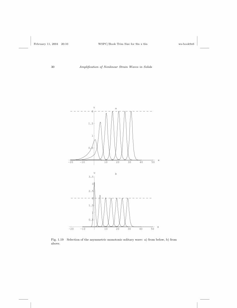
this another way, the parameters of the resulted steady wave are selected.Selection provided by an amplification of an initial wave, will be calledselection from below, see Fig. 1.17(a), while selection from above happensas a result of an attenuation of an initial wave, see Fig. 1.17(b).
Shown in Fig. 1.18 is the profile of the wave (1.34) in comparison withthe symmetric solitary wave solution (1.33) at t = 0. One can see that thewave (1.34) is asymmetric with respect to its core (or maximum). However,only initial stages of the temporal evolution of (1.34) differs from that ofEq.(1.33). As follows from Fig. 1.19, the final stage of the selection bothfrom below and above, is the symmetric bell-shaped solitary wave like shownin the last stages in Fig. 1.17.
The amplification/attenuation of the kink may be described asymp-totically and numerically Sachdev (1987), it will be shown in Sec. 5.3.Cnoidal wave evolution may be accounted for an asymptotic solutionsimilar to that of the bell-shaped solitary waves Rednikov et. al (1995);Svendsen and Buhr-Hansen (1978).
February 11, 2004 20:10 WSPC/Book Trim Size for 9in x 6in ws-book9x6
30 Amplification of Nonlinear Strain Waves in Solids
-20 -10 10 20 30 40 50x
0.5
1
1.5
2
2.5
3
3.5
u b
-20 -10 10 20 30 40 50x
0.5
1
1.5
2
u a
Fig. 1.19 Selection of the asymmetric monotonic solitary wave: a) from below, b) fromabove.

February 11, 2004 20:10 WSPC/Book Trim Size for 9in x 6in ws-book9x6
Chapter 2
Mathematical tools for the governingequations analysis
As a rule governing equations for nonlinear strain waves are nonitegrableby the inverse scattering transform method, and only particular analyticalsolutions may be obtained. Hence the study of real physical processesrequires a combined analytico-numerical approach. The aim of this chapteris to describe methods to be used in this book. The choice of the analyticaland numerical procedures is based on an experience of the author and doesnot claim a completeness.
2.1 Exact solutions
2.1.1 Direct methods and elliptic functions
Most of the mathematical work in the realm of nonlinear phenomenarefers to integrable equations and their exact solutions, particularly, pe-riodic. Among the recently developed general methods the algebroge-ometrical approach may be used in an efficient way to find such solu-tions. Not only the numerical realization and graphical representation ofthe solution is provided by this method but also multi phase quasiperi-odic solutions as well as purely periodic ones may be represented usingthe algebrogeometrical approach as illustrated in Belokolos et. al (1994).When we are interested in a self-similar solution of a partial differentialequation one can use well developed theory of the solutions of ordinarydifferential equations, see, e.g., Ince (1964). Exact solutions of nonlin-ear nonintegrable partial differential equations are obtained usually us-ing various direct methods. The significant point in direct methods is tobuild in advance the appropriate functional form of the solution (ansatz)of the equation studied. For example, the usage of ansatz in the form
31

February 11, 2004 20:10 WSPC/Book Trim Size for 9in x 6in ws-book9x6
32 Amplification of Nonlinear Strain Waves in Solids
of a hyperbolic tangent (tanh) power series resulted in finding of newexact travelling wave solutions (see, e.g., Korpel and Banerjee (1984);Parkes and Duffy (1996) and references therein). The choice of tanhis caused by the fact that any derivatives of tanh may be expressed asa polynomial with respect to the tanh itself. Then the equation stud-ied becomes polynomial of the tanh after substituting the ansatz, andsolution parameters are obtained from the algebraic equations appear-ing after equating to zero coefficients at each order of tanh . One wouldlike to apply the same procedure to find more general periodic solutions.First of all another appropriate ”basic” function is required instead of thetanh . For this purpose various elliptic functions were proposed recently,the most popular were theta functions (see, e.g.,Chow (1995), Nakamura(1979)), Jacobian elliptic functions (see, e.g.,Kostov and Uzunov (1992);Parker and Tsoy (1999)) and the Weierstrass elliptic function Kascheev(1990); Porubov (1993); Porubov (1996); Porubov and Parker (2002);Samsonov (1995); Samsonov (2001). In principle, periodical solutions couldbe obtained in terms of any of these functions. The efficient choice is causedby the simplest procedure of the ansatz construction and the least compli-cated algebra for determining solution parameters. It is well known thattheta functions may be included in the Hirota bilinear method in order toget N-periodical solutions Nakamura (1979). However most of dissipativeequations cannot be transformed to the bilinear form. At the same timesingle travelling wave solution derivation looks very complicated even fornon-dissipative equations Chow (1995), Nakamura (1979). Moreover wehave to deal with four theta functions that results in additional difficul-ties for the ansatz construction. Explicit periodic travelling wave solutionsmay be found for many nonintegrable equations and systems by using anansatz in terms of ℘, with appropriate forms for the ansatz suggested byinformation about the poles of the solution. When compared to the useof theta functions or Jacobi elliptic functions, a prime advantage of usingthe function ℘ is that the algebra is drastically simplified. The ansatz forthe solution involves only one Weierstrass function ℘(ζ, g2, g3), instead offour theta functions or three Jacobi elliptic functions cn(ζ, k), sn(ζ, k)and dn(ζ, k). Another advantage is that two apparently distinct solutionsare readily recognized as equivalent. In order to see it let us first givesome properties of the Weierstrass elliptic function ℘ to be used below.According to its definition Whittaker and Watson (1927), the Weierstrassfunction is analytical in the complex plane other than in the points where
February 11, 2004 20:10 WSPC/Book Trim Size for 9in x 6in ws-book9x6
Mathematical tools for the governing equations analysis 33
it has double poles. The governing equation for the function ℘ is:
℘′(ζ)2 = 4℘3 − g2℘− g3 (2.1)
where g2 and g3 are constant parameters. Remarkable features of the func-tion ℘ are that all of its derivatives can be written by means of itself,and that any elliptic function f may be expressed using ℘ it and its firstderivative as Whittaker and Watson (1927)
f = A(℘) + B(℘)℘′, (2.2)
where A and B are rational functions with respect to ℘. Depending onthe ratio between g2 and g3 the Weierstrass function may be bounded orunbounded inside the domain under study. The bounded periodic solutionsare more conveniently expressed by writing them in terms of the Jacobielliptic functions cn, sn and dn which are bounded on the real axis. Forthis purpose the relation between the Weierstrass function and the Jacobianfunctions is used as a special case of (2.2). Indeed, the familiar link isobtained in Whittaker and Watson (1927) but using the singular functionsn−2,
℘(ζ, g2, g3) = e3 + (e1 − e3)sn−2(√
e1 − e3ζ, k). (2.3)
However, following the method introduced in Whittaker and Watson (1927)one can check that the following formula is valid:
℘(ζ, g2, g3) = e2 − (e2 − e3)cn2(√
e1 − e3ζ, k), (2.4)
connecting the Weierstrass function with the Jacobi function cn, regularalong the real axes. Here k =
√(e2 − e3)/(e1 − e3) is the modulus of the
Jacobian elliptic function, while τ = em (m = 1, 2, 3 , e3 ≤ e2 ≤ e1 ) arethe real roots of the cubic equation
4τ3 − g2τ − g3 = 0. (2.5)
Expressing these results in terms of an appropriate choice of parameters,the wave number κ =
√e1 − e3 and the Jacobian elliptic modulus k, we
have
e3 = −1 + k2
3κ2, e2 =
2k2 − 13
κ2, e1 =2− k2
3κ2,

February 11, 2004 20:10 WSPC/Book Trim Size for 9in x 6in ws-book9x6
34 Amplification of Nonlinear Strain Waves in Solids
g2 =83κ4(1− k2 + k4), g3 =
427
κ6(k2 + 1)(2− k2)(1− 2k2). (2.6)
The localized both the bells-shaped and the kink-shaped solitary wave so-lutions appear in the limit k → 1 of the Jacobi elliptic functions.
Now consider an instructive example Porubov and Parker (2002). InParker and Tsoy (1999), solutions were sought in terms of powers andproducts of Jacobi functions and thereby two solutions were obtained
z1 = e2 − (e2 − e3) cn2(√
e1 − e3ζ, k), (2.7)
z2 =r2m2
2sn2(rζ, m)± r2m
2cn(rζ, m)dn(rζ, m)− r2(1 + m2)
12, (2.8)
which appear different. Obviously, the solution (2.7) is a representation ofthe Weierstrass function (2.3). However, one can check by direct substitu-tion that the solution (2.8) also satisfies equation (2.1) when the parametersr and m are defined as solutions to
r4
12(1 + 14m2 + m4) = g2 ,
r6
216(1− 33m2 − 33m4 + m6) = g3. (2.9)
Therefore z2 is also a solution satisfying the same governing equation(2.1) defining the Weierstrass function. The two expressions (2.7) and (2.8)are essentially equivalent solutions, provided that (r, m) are appropriatelyrelated to (r, k). Accordingly, working with ℘ reveals links between seem-ingly distinct forms of solution.
It is to be noted that the first Weierstrass function derivative ℘′ can-not be expressed as a polynomial of the Weierstrass function itself Whit-taker and Watson (1927), and we have to equate zero separately coeffi-cients at each order of ℘ and at products of ℘′ and corresponding ordersof ℘ Kascheev (1990); Porubov (1993); Porubov (1996); Samsonov (1995);Samsonov (2001). Therefore we really deal with two functions, and it isunlikely to get the solution using the ansatz proposed in the form of powerseries with respect both of the ℘ and ℘′ as it was done for the tanh. An-other idea may be used, based on the singular point analysis of the possiblesolution and the well known fact that the Weierstrass function ℘ has thesecond order poleWhittaker and Watson (1927). In order to check the polesof a solution we shall use the WTK method Weiss et. al (1983) looking forthe solution in the form of Laurent- type series about the singular manifold.It will be explained in details in Sec. 2.1.2.

February 11, 2004 20:10 WSPC/Book Trim Size for 9in x 6in ws-book9x6
Mathematical tools for the governing equations analysis 35
The exact solutions obtained in this manner, usually belong to the classof travelling wave solutions which require special initial conditions. In caseof the solitary wave solution the initial condition should be have the shapeof the solitary wave itself. Moreover, travelling wave solutions for the dis-sipative equations usually have not free parameters, and additional rela-tionships on the equation coefficients are required for the existence of thesolutions Porubov (1993); Porubov (1996); Porubov and Velarde (1999);Porubov and Parker (1999); Porubov and Parker (2002); Samsonov (1995);Samsonov (2001).
2.1.2 Painleve analysis
Recently it was developed the theory of nonlinear ordinary differentialequations whose solutions have not movable singularities, other than poles.Then the theory has been extended to partial differential equations. Usuallythese equations are called ”equations with the Painleve property”. Theachievements of the theory may be found in Cariello and Tabor (1989);Conte (1989); Conte et. al (1993); Levi and Winternitz (1992); Newell et. al(1987); Weiss et. al (1983). Here we concentrate on the one aspect of thetheory-the singular manifold method or WTC method for partial differen-tial equations Newell et. al (1987); Weiss et. al (1983). Let ϕ(x, t) = 0 isthe ”singular” or ”pole” manifold on which a solution u(x, t) is singular.The main idea of the WTC is to demonstrate that the expansion
u(x, t) =1
ϕα
∞∑
j=0
qj(x, t)ϕj (2.10)
is single valued. This requires (i) α is an integer, (ii) ϕ is analytic in x
and t and (iii) the equations for the coefficients qj have self-consistentsolutions. When all these conditions are satisfied the equation under studyhas the Laurent property. Also it is necessary to assume that neither ϕx
nor ϕt vanish on ϕ(x, t) = 0. Let us illustrate how the methods workson an example of the KdV equation (1.1). Following Newell et. al (1987);Weiss et. al (1983) we assume b = 3, d = 1. Substituting the ansatz (2.10)into Eq.(1.1) one can find α = 2 and q0 = −2ϕ2
x. Recursion relations forthe qj are
(j + 1)(j − 4)(j − 6)qj = F (ϕt, ϕx, ..., qk; k < j). (2.11)
The values of j, j = −1, 4 and 6 are called resonances. At each such

February 11, 2004 20:10 WSPC/Book Trim Size for 9in x 6in ws-book9x6
36 Amplification of Nonlinear Strain Waves in Solids
resonance the right-hand side of Eq.(2.11) vanishes thus ensuring the inde-terminancy of the corresponding qj . Moreover, the expansion (2.10) maybe truncated at O(ϕ0). As a result we obtain using Eq.(2.11) an auto-Backlund transformation for the solution of Eq.(1.1),
u(x, t) = 2∂
∂x2log ϕ + q2,
where q2 satisfies the KdV equation. Also the Lax pair for the KdV equationfollows from the solution of Eq.(2.11) Newell et. al (1987); Weiss et. al(1983).
However, the Lax pair cannot be obtained for nonitegrable equations asopposed to a truncated expansion that carries an information about possiblepole orders of a solution. Using this information the anzats for the solutionmay be proposed, in particular, in terms of the Weierstrass elliptic function℘ and ℘′. Substituting the proposed form of the solution into the equationunder study and equating to zero coefficients at each order of ℘ and at prod-ucts of ℘′ and corresponding orders of ℘ one can get the algebraic equationson the solution parameters, the phase velocity and the Weierstrass functionparameters g2, g3. Certainly this procedure is of phenomenological kindbut it allows to obtain the solutions of nonitegrable nonlinear equations inan explicit form. Some examples are presented below.
2.1.3 Single travelling wave solutions
First we consider exact solutions of DMKdV Eq.(1.13) obtained in Porubov(1993). It was found there the following auto-Backlund transformation forthe solution u(x, t)
u =12
∼α4
∼α5
(log ϕ)xx +12
5∼α5
(α3 − 2α1∼α4
∼α5
)(log ϕ)x+∼u, (2.12)
where∼u (x, t) satisfies Eq.(1.13). Concerning only tavelling wave solutions,
one can reduce Eq.(1.13) to the third-order ODE of the form:∼α4 u′′′ + α3 u′′+
∼α2 u′+
∼α5 uu′ + α1 u2 − V u + P = 0, (2.13)
where P = const, prime denotes differentiation with respect to θ, θ = x−V t. Based on Eq.(2.12) possible solution may contain simple and second-order poles that may be modelled in terms of ℘ as Porubov (1993):
u = A℘ +B℘′
℘ + C+ D. (2.14)

February 11, 2004 20:10 WSPC/Book Trim Size for 9in x 6in ws-book9x6
Mathematical tools for the governing equations analysis 37
Substituting Eq.(2.14) into Eq.(2.13) one can derive a system of alge-braic equations in A, B, C, D, phase velocity V and Weierstrass functionparameters g2, g3:
(g2C − g3 − 4C3)B = 0, (12C2 − g2)B = 0,
P = V D + 8α1B2C − α1D
2 − α3g2A/2− 2∼α2 BC + 12
∼α4 BC2 −
∼α5 (2ABC2 + g2AB/2− 2BCD),
2α1(2B2 + AD)− V A + 2∼α2 B + 2
∼α5 (BD −ABC) = 0,
α1A2 + 6α3A + 12
∼α4 B + 6
∼α5 AB = 0,
B(2α1(D −AC)− V ) = 0, A(12∼α4 +
∼α5 A) = 0,
2α1AB + 2α3B+∼α2 A+
∼α5 (AD + 2
∼α5 B2) = 0.
The solutions of these equations are:(i) when g2, g3 are free parameters and α3 = 2α1
∼α4 /
∼α5;
A = −12∼α4∼α5
, B = 0, D = −∼α2∼α5
, V = −2α1∼α2
∼α5
.
(ii) when either
C = − 1
300∼α4
2 (α3 − 2α1∼α4
∼α5
)2,
or α3 = 12α1∼α4 /
∼α5, C is a free parameter
A = −12∼α4∼α5
, B = − 6
5∼α5
(α3 − 2α1∼α4
∼α5
),
D = −∼α2∼α5
+2α1
∼α5
2 (α3 − 2α1∼α4
∼α5
) +1
25∼α4
∼α5
(α3 − 2α1∼α4
∼α5
)2,
V =24α1
∼α4
∼α5
C − 2α1∼α2
∼α5
+4α2
1
∼α5
2 (α3 − 2α1∼α4
∼α5
) +
2α1
25∼α4
∼α5
(α3 − 2α1∼α4
∼α5
)2, g2 = 12C2, g3 = 8C3.

February 11, 2004 20:10 WSPC/Book Trim Size for 9in x 6in ws-book9x6
38 Amplification of Nonlinear Strain Waves in Solids
Using (2.4) the solution (2.14) with parameters defined by (i) may de-scribe a particular bounded cnoidal wave, propagating with fixed phasevelocity, of the form:
u =12
∼α4∼α5
k2κ2cn2(kθ, κ)−∼α2∼α5
− 4∼α4∼α5
k2(2κ2 − 1) (2.15)
where k is a free parameter. When the Jacobian elliptic functions modulusκ → 1 the solution (2.15) transforms to the solitary wave solution (1.12).The solution (2.14) with parameters defined by (ii) accounts for a boundedkink-shaped solution (1.28). When C is a free parameter, kink propagateswith any phase velocity value.
Besides bounded solutions (2.15) and (1.28), the solution (2.14) alsodescribes unbounded ones in the form of localized and periodic discontinu-ities. Finally it is to be noted that the functional form (2.14) in terms ofthe Weierstrass function is not unique. One can see that there exist at leastone more solution of the form:
u = − 12
25∼α4
∼α5
(α3 − 2α1∼α4
∼α5
)2 exp(2y)℘(exp(y) + G, 0, g3),
where
y = exp(γθ), γ = − 1
5∼α4
(α3 − 2α1∼α4
∼α5
),
G and g3 are free parameters. This solution allows to describe only thebounded kink-shaped wave (1.28). At the same time it accounts for a newperiodically discontinious solution.
In previous Chapter the bounded periodic solution (1.32) of the equa-tion (1.31) was considered. When studying travelling wave solutions, i.e.solutions depending only on the phase variable θ = x− V t, this equationmay be transformed into the O.D.E., which results in the following equationafter integrating once with respect to θ:
dη′′′ + gη′′ − V η′ + b(η2)′ + f(η2)′′ + c(η3)′ = N. (2.16)
Further we follow the results obtained in Porubov (1996). The transforma-tion is obtained here using the WTK method of the form
u =f ±
√f2 − 2cd
c(log ϕ)′ + u. (2.17)

February 11, 2004 20:10 WSPC/Book Trim Size for 9in x 6in ws-book9x6
Mathematical tools for the governing equations analysis 39
Therefore possible solution should contain first order pole. The Weierstrasselliptic function ℘ possesses second order pole, and we shall propose threesolution forms. The first of them is
u =A℘′
℘ + C+ B. (2.18)
In order to find the solution parameters the formula (2.18) is substitutedinto the Eq.(2.16). Then equating to zero coefficients at each order of ℘+C
and ℘′ one can derive the algebraic equations on A,B, C, phase velocity V
and the Weierstrass function parameters g2, g3:
(℘ + C)−4 : (g2C − g3 − 4C3)2(6Af − 3A2c− 6d) = 0,
(℘ + C)−3 : (g2C − g3 − 4C3)(12C2 − g2)(14Af − 9A2c− 12d) = 0,
(℘ + C)−2 : 4(g2C − g3 − 4C3)(2bB − V + 48ACf + 3c(12A2C −B2)− 48Cd)− 3(12C2 − g2)2(2f − 2Ac− d) = 0,
(℘ + C)−1 : 4(g2C − g3 − 4C3)(10f − 4f + 3Ac + 6d)− (12C2 −g2)(2Bb− V + 24ACf + 3(B2 − 12A2C)c− 12Ad) = 0,
℘0 : 4(12C2 − g2)qA2 = N,
(℘ + C) : 2Bb− V + 24ACf + 6(B2 − 12A2C)c− 12Cd = 0,
(℘ + C)2 : 2Af + d + 2A2c = 0,
℘′(℘ + C)−3 : (g2C − g3 − 4C3)(g + 2Bf −Ab− 3ABc) = 0,
℘′(℘ + C)−2 : (12C2 − g2)(2Ab− g − 2Bf + 6ABc) = 0,
℘′ : 2Ab + g + 2Bf + 6ABc = 0.
Three solutions of algebraic equations are obtained. The first appearswhen
12C2 − g2 = 0, g2C − g3 − 4C3 = 0.
In this case two of three roots ei of Eq.(2.5) are equal to one another, andno periodical solution exists. Then the solution (2.18) will have the formof localized discontinuity under positive C values. When the parameter C
is negative we get κ = 1, and the bounded kink-shaped solitary wavesolution follows from Eq.(2.18):
u = γ tanh(mθ) + u0. (2.19)
For the wave amplitude γ two formulaes are valid
γ = A1m, A1 = (f + (f − 2cd)1/2)/(6c),

February 11, 2004 20:10 WSPC/Book Trim Size for 9in x 6in ws-book9x6
40 Amplification of Nonlinear Strain Waves in Solids
γ = A2m, A2 = (f − (f − 2cd)1/2)/(6c).
Then for u0 we have
u0 =2bAj − g
2(3cAj + f), j = 1, 2,
and phase velocities V1, V2 are
V1 = 2u01b + 6c(u201 + 4A2
1m2)− 4m2(2fA1 − d),
V2 = 2u02b + 6c(u202 + 4A2
2m2)− 4m2(2fA2 − d),
while m2 = −3C = 3e1 is a free parameter.The second solution corresponds to the situation when
g2C − g3 − 4C3 = 0, 12C2 − g2 6= 0. (2.20)
In this case the solution may exist under additional conditions on the equa-tion coefficients f = g = 0, that results in absence of the dissipative termsin Eq.(2.16). Hence it becomes now the O.D.E. reduction of the Gardnerequation. The bounded cnoidal wave solution arises when C = −e1 andhas the form
u = ±√−2d
cκ2m
cn(mθ, κ)sn(mθ, κ)dn(mθ, κ)
− b
3c, (2.21)
where m2 = e1 − e3. It governs the travelling cnoidal wave, propagatingwith the phase velocity V = −b2/(3c) − 6e1d. that transforms into thekink-shaped soluiton (2.19) when κ = 1.
Finally, the third solution arises when
12C2 − g2 = 0, g2C − g3 − 4C3 6= 0.
In this case the bounded cnoidal wave solution (1.32) holds. When κ = 1we have C∗ = 0, and it transforms into the kink-shaped solution (2.19), seeFig. 1.6.
Now we shall consider the second possible solution’s form in terms ofthe Weierstrass elliptic function ℘:
η =√
A℘ + B. (2.22)
Substitution Eq.(2.22) into the Eq.(2.16) allows us to conclude that solutionmay now exist only when f = g = 0. Then one can get the algebraic

February 11, 2004 20:10 WSPC/Book Trim Size for 9in x 6in ws-book9x6
Mathematical tools for the governing equations analysis 41
equations for the solution parameters equating to zero coefficients at theterms ℘′ ℘k, k = 0÷ 3, and (A℘ + B)5/2:
℘′ ℘3 : cA + 2d = 0
℘′ ℘2 : 9cAB − V A + +15dB = 0
℘′ ℘ : 9cAB − 2V A + +12dB = 0
℘′ : 12cB3 − 4V B2 + dA(Bg2 −Ag3) = 0
(A℘ + B)5/2 : N = 0
One can obtain the following solution of these equations:
A = − 2d
c, B =
2dei
c, i = 1÷ 3, V = − 1
2cB,
where ei are the real roots of Eq. (2.5). We again deal with the O.D.E.reduction of the Gardner equation, however now one can obtain its anotherbounded solutions. Thus for d/fc > 0 we find cnoidal wave solutions ofthe form:(I) for B = 2de2/c
u =
√2d
cm κ cn(mθ, κ), (2.23)
where m2 = e1−e3 and for the phase velocity we have V = dm2(2κ2−1).(II) for B = 2de1/c we obtain
u =
√2d
cm κ dn(mθ, κ), (2.24)
Solution (2.24) represents cnoidal wave propagating with the phase velocityV = dm2(2 − κ2). It is to be noted that at κ = 1 both the solutions(2.23) and (2.24) transform to the bell-shaped solitary wave
u =
√2d
cm ch−1(mθ, κ),
propagating with the velocity V = dm2.When d/c > 0 the bounded solution appears from (2.22) if B = 2de3/c
and has the form
u =
√2d
cm κ sn(mθ, κ), (2.25)

February 11, 2004 20:10 WSPC/Book Trim Size for 9in x 6in ws-book9x6
42 Amplification of Nonlinear Strain Waves in Solids
For the phase velocity we find V = −dm2(1+κ2). In contrast to solutions(2.23), (2.24) the solution (2.25) transforms to the kink-shaped solution(2.19) when κ = 1.
Finally one can construct the third possible solution in terms of theWeierstrass elliptic function ℘ depending now on new independent variabley = exp(kθ). Changing variable in auto-Backlund transformation (2.17)one can see that the following solution may be proposed:
u = Ay℘′y
℘ + C+ B, (2.26)
Substituting it into Eq.(2.16) one can find that solution may exist underf = 0. Therefore we now deal with the O.D.E. reduction of the Gardnerequation with linear dissipation. The solution of the form (2.26) for thelast equation was already obtained previously in Samsonov (1995). It wasfound that this solution may correspond either to discontinuous periodicalsolution or to the bounded kink-shaped solution of the form similar to thesolution (2.19).
2.1.4 Exact solutions of more complicated form
The procedure of the obtaining exact solutions is based on the reductionto the ODE, hence only travelling wave solutions may be found. However,sometimes this procedure is applied to obtain only the part of a solution,and more complicated profiles are decsribed. Consider some examples.Recently the coupled nonlinear Schrodinger equations (CNLS)
iWt + sWxx + (ηWW ∗ + σUU∗)W = 0,
iρUt + rUxx + (η−1UU∗ + σWW ∗)U = 0, (2.27)
with r, s = ±1; ρ, σ, η real, have attracted considerable interest becauseof their role in governing various physical wave-guiding systems. Theseequations are not generally integrable by the inverse scattering transformmethod, except in cases of high symmetry (e.g. ρ = 1, η = σ = ±1). Themachinery of the Weierstrass function is applied in the search for travellingwave solutions of equations (2.27) in the form
W = w(ζ) eiζ , U = u(ζ) eiφ, (2.28)
where θ = x− c t, ζ = ζ(θ, t), φ = φ(θ, t), with u,w, ζ and φ real. Substitu-tion (2.28) into equations (2.27) allows to separate the real and imaginary
February 11, 2004 20:10 WSPC/Book Trim Size for 9in x 6in ws-book9x6
Mathematical tools for the governing equations analysis 43
parts. The solutions for u and w are sought in the form
w =√
F℘2 + A℘ + B, u =√
G℘2 + D℘ + E, (2.29)
while for ζ and φ we have
ζ = 12s c θ − sC1
∫dθ
w2+ ζ0(t) ,
φ = 12r c ρ θ − r C2
∫dθ
u2+ φ0(t) , (2.30)
where Ci (i = 1, 2) are free parameters. The most notable difference fromprevious solutions is the dependence of the “frequency” and “phase” on w
and u, when Ci 6= 0. This introduces significant features into the profilesof the real and imaginary parts of W and of U . Thus, we find for W of theform:
W = w exp ı Y, (2.31)
where w is defined by Porubov and Parker (1999)
w =
√A
2k2 − 1
3κ2 − k2κ2cn2(κθ, k) + B/A
, (2.32)
while for the phase function Y we have
Y =csθ
2− sC1Π[ϕ, n, k]
κA(H1 − e3)+ (γ +
c2s
4)t, (2.33)
Π[ϕ, n, k] is the elliptic integral of the third kind, ϕ = arcsin(sn(κθ)), n =−κ2k2/(B/A + e3) and C1 is defined by
A =2(σ r η − s)η(1− σ2)
, C21 =
A2
4
4
(B
A
)3
− g2B
A+ g3
, (2.34)
γ =σ(E A−B D)− 3sB
A,D =
2(s σ − r η)1− σ2
,
where B, E, g2 and g3 are free parameters. The shape of the wave (2.31)depends strongly on the values of the parameters κ, k and H1. An exampleof the behavior of Re W is shown in Fig.2.1(a) for the case H1 ∈ [e2, e3], c ∼κ and at t = 0. We get an interesting wave, consisting of the carrier waveslightly modulated and with superposed periodic disturbances. Therefore,

February 11, 2004 20:10 WSPC/Book Trim Size for 9in x 6in ws-book9x6
44 Amplification of Nonlinear Strain Waves in Solids
20 40 60 80 100x
-2
-1
1
2
Re W b
20 40 60 80 100x
-2
-1
1
2
Re W a
Fig. 2.1 Exact solutions of the CNLS. a) profile with moving disturbances; b) almostenvelope wave solution.
the wave shape is not determined solely by the amplitude wave shape.When c considerably exceeds the wave number κ we get the profile closerto the usual envelope wave solution, see Fig. 2.1(b).
Another interesting profiles correspond to the exact solutions of the

February 11, 2004 20:10 WSPC/Book Trim Size for 9in x 6in ws-book9x6
Mathematical tools for the governing equations analysis 45
complex Ginzburg-Landau equation, CGLE,
ı ut + p uxx + q |u|2 u = ı γ u (2.35)
where the constant coefficients are p = pr+ı pi, q = qr+ı qi, with pj , qj 6= 0,(u, p, q) ∈ C, γ ∈ R. The subscripts t and x denote temporal and spatialderivatives, respectively. This equation appears in the description of a largevariety of physical phenomena, e.g., in nonlinear optics, non-equilibriumpattern formation, lasers, superconductivity etc. Like in case of CNLSequations, first of all, we decompose the solution u(x, t) in its amplitude,y, and phase, θ, both real,
u = y(ζ) eıθ, (2.36)
where ζ = x− c t, θ = θ(ζ, t). Substituting (2.36) into (2.35) and equatingto zero the real and imaginary parts one obtains two coupled equations forthe functions y and z ≡ θζ . Then periodic and pulse solutions of the CGLEmay be found Porubov and Velarde (1999). The first derivative of the realpart of the periodic solution with respect to x, v = (Reu)x, is
v =Z
ysin
(θ + arcsin(
y yx
Z))
, (2.37)
with
y =√
2qr
pr
k21dn2(k1ζ, κ)− δ2
1
, Z =
√y2y2
x + C2. (2.38)
When C = 0, the zeroes of the first derivative (2.37) are defined bythe zeroes of the function yx and correspond to the zeroes of the Jacobifunctions cn and sn. Their positions do not change in time, and for u wehave harmonic temporal oscillations of the spatially periodic state definedby the amplitude parts of the solutions (2.36). However, the situationchanges dramatically when C 6= 0. In this case Z never vanishes, and thezeroes of the first derivative are defined by the zeroes of the sin functiononly, whose position vary in time. A typical situation is shown in Fig. 2.2.Fig. 2.2(a) shows a structure with four spatially repeated parts. During halfof the time period the shapes of these parts vary, and we get in Fig. 2.2(d)a profile which is practically the mirror image to Fig. 2.2(a). Qualitativelythis evolution does not depend upon the value of the modulus κ of Jacobifunctions.
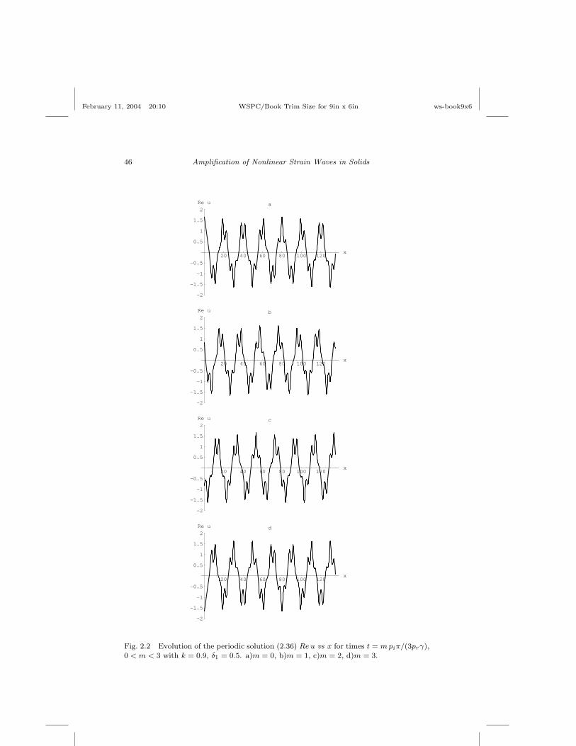
February 11, 2004 20:10 WSPC/Book Trim Size for 9in x 6in ws-book9x6
46 Amplification of Nonlinear Strain Waves in Solids
20 40 60 80 100 120x
-2
-1.5
-1
-0.5
0.5
1
1.5
2
Re u d
20 40 60 80 100 120x
-2
-1.5
-1
-0.5
0.5
1
1.5
2
Re u c
20 40 60 80 100 120x
-2
-1.5
-1
-0.5
0.5
1
1.5
2
Re u b
20 40 60 80 100 120x
-2
-1.5
-1
-0.5
0.5
1
1.5
2
Re u a
Fig. 2.2 Evolution of the periodic solution (2.36) Re u vs x for times t = m piπ/(3prγ),0 < m < 3 with k = 0.9, δ1 = 0.5. a)m = 0, b)m = 1, c)m = 2, d)m = 3.
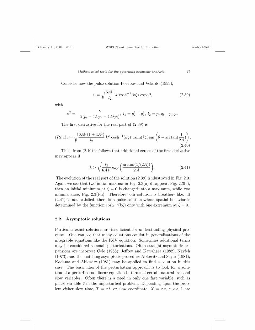
February 11, 2004 20:10 WSPC/Book Trim Size for 9in x 6in ws-book9x6
Mathematical tools for the governing equations analysis 47
Consider now the pulse solution Porubov and Velarde (1999),
u =√
6Al1l2
k cosh−1(kζ) exp ıθ, (2.39)
with
κ2 = − γ
2(pi + 4Apr − 4A2pi), l1 = p2
r + p2i , l2 = pr qi − pi qr.
The first derivative for the real part of (2.39) is
(Re u)x =
√6Al1(1 + 4A2)
l2k2 cosh−1(kζ) tanh(kζ) sin
(θ − arctan(
12A
))
.
(2.40)Thus, from (2.40) it follows that additional zeroes of the first derivative
may appear if
k >
√l2
6A l1exp
(arctan(1/(2A))
2 A
). (2.41)
The evolution of the real part of the solution (2.39) is illustrated in Fig. 2.3.Again we see that two initial maxima in Fig. 2.3(a) disappear, Fig. 2.3(e),then an initial minimum at ζ = 0 is changed into a maximum, while twominima arise, Fig. 2.3(f-h). Therefore, our solution is breather- like. If(2.41) is not satisfied, there is a pulse solution whose spatial behavior isdetermined by the function cosh−1(kζ) only with one extremum at ζ = 0.
2.2 Asymptotic solutions
Particular exact solutions are insufficient for understanding physical pro-cesses. One can see that many equations consist in generalisations of theintegrable equations like the KdV equation. Sometimes additional termsmay be considered as small perturbations. Often straight asymptotic ex-pansions are incorrect Cole (1968); Jeffrey and Kawahara (1982); Nayfeh(1973), and the matching asymptotic procedure Ablowitz and Segur (1981);Kodama and Ablowitz (1981) may be applied to find a solution in thiscase. The basic idea of the perturbation approach is to look for a solu-tion of a perturbed nonlinear equation in terms of certain natural fast andslow variables. Often there is a need in only one fast variable, such asphase variable θ in the unperturbed problem. Depending upon the prob-lem either slow time, T = ε t, or slow coordinate, X = ε x, ε << 1 are

February 11, 2004 20:10 WSPC/Book Trim Size for 9in x 6in ws-book9x6
48 Amplification of Nonlinear Strain Waves in Solids
-0.04 0.04 x
-4
-2
2
4
Re u g
-0.04 0.04 x
-4
-2
2
4
Re u h
-0.04 0.04 x
-4
-2
2
4
Re u e
-0.04 0.04 x
-4
-2
2
4
Re u f
-0.04 0.04 x
-4
-2
2
4
Re u c
-0.04 0.04 x
-4
-2
2
4
Re u d
-0.04 0.04 x
-4
-2
2
4
Re u a
-0.04 0.04 x
-4
-2
2
4
Re u b
Fig. 2.3 Evolution of the pulse solution (2.39) Re u vs x for times t = mπ/β, 0 < m < 8.a)m = 0, b)m = 1, c)m = 2, d)m = 4, e)m = 5, f)m = 6, g)m = 7, h)m = 8.
introduced. Fast variable is generalized in a perturbed problem assumingeither θx = 1, θt = −V (T ) or θx = P (X), θt = −1. The functions V (T )or P (X) are defined to remove secular terms. Some of the appropriate sec-ularity conditions are formed from Green’s identity as follows. Assume asolution u = u(θ, T ) is of the form

February 11, 2004 20:10 WSPC/Book Trim Size for 9in x 6in ws-book9x6
Mathematical tools for the governing equations analysis 49
u(θ, T ) = u0(θ, T ) + ε u1(θ, T ) + ... (2.42)
The leading order problem is nonlinear equation for u0 whose solutionis known. Then in the next order an inhomogeneous linear equation for u1
holds
L(u1) = F (u0).
Here L(u1) is a linearized leading-order equation operator. Denoting byvi(i = 1, ..., M) the M solutions of the homogeneous adjoint problem,
LA(vi) = 0, i = 1, ..., M,
where LA is the adjoint operator to L, we obtain that
L(u1)vi − LA(vi)u1 = Fvi
is always a divergence. Using the boundary conditions it may be integratedto give the secularity conditions. In particular, when vi → 0 as |θ| → ∞while u1 is bounded the secularity condition is:
∫ ∞
−∞viF dθ = 0. (2.43)
Then either V (T ) or P (X) are obtained from Eq.(2.43). Method maybe used for finding perturbed cnoidal wave solutions. In this case in-tegration in (2.43) is carrying over the period Rednikov et. al (1995);Svendsen and Buhr-Hansen (1978). It is to be noted that a simple qua-sistationary expansion is not uniformly valid on |x| → ∞. Completesolutions is obtained using matching quasistationary solution to a non-stationary one for large |θ|, e.g. |θ| ∼ 1/ε Ablowitz and Segur (1981);Kodama and Ablowitz (1981).
Let us apply this method for a perturbed solitary wave solution of theDMKdV equation (1.13). Following Kliakhandler et. al (2000); Rednikovet. al (1995) assume that
∼αi= ε α i, ε << 1, and suppose that u depends
upon a fast variable θ and a slow time T , such as
θx = 1, θt = −V (T ), T = ε t.
Then equation (1.13) becomes
α3 uθθθ − V uθ + 2α1 u uθ + ε [uT + α2 uθθ + α4 uθθθθ + α5 (uuθ)θ] = 0.
(2.44)

February 11, 2004 20:10 WSPC/Book Trim Size for 9in x 6in ws-book9x6
50 Amplification of Nonlinear Strain Waves in Solids
The solution of Eq.(2.44) is sought in the form (2.42). In the leadingorder we get
α3 u0,θθθ − V u0,θ + 2α1 u0 u0,θ = 0. (2.45)
We are interested in studying localized solutions vanishing together withits derivatives at |θ| → ∞. Then the leading order solution is
u0 =6 α3
α1b(T )2 cosh−2 (b(T ) θ) (2.46)
with V = 4α3 b2. At order ε, we have
α3 u1,θθθ − V u1,θ + 2α1 (u 0u1)θ = F, (2.47)
F = − [u0,T + α2 u0,θθ + α4 u0,θθθθ + α5 (u0 u0,θ)θ
].
The operator acting on the function u1 in the lhs of Eq.(2.47) is adjoint tothat of the Eq.(2.45). Then the secularity condition (2.43) with vi = u0
yields the equation for b:
bT =815
b3(A + B b2
), (2.48)
with
A = α2, B =47
(6α3α5
α1− 5α4
). (2.49)
The behavior of b (or the sign of bT ) depends on the signs of A andB and on the value of b0 ≡ b(T = 0). Indeed, when both A and B
are positive b diverges while for both negative values it will vanish. ForA < 0, B > 0 the parameter b vanishes if b0 <
√−A/B while it diverges
if b0 >√−A/B. The most interesting case occurs when A > 0, B < 0.
Here b tends to√−A/B independent of b0. A quantitative description of
the variation of b can be given. Equation (2.48) may be directly integratedgiving the implicit dependence of b on T :
T =4 B
15A2ln
∣∣∣∣b20(A + B b2)
b2(A + B b20)
∣∣∣∣−4(b2
0 − b2)15Ab2 b2
0
. (2.50)
We see that b tends to infinity in finite time, T = T ∗ for A > 0, B > 0,
T ∗ =4 B
15A2ln
b20B
(A + B b20)
+4
15A b20
, (2.51)
February 11, 2004 20:10 WSPC/Book Trim Size for 9in x 6in ws-book9x6
Mathematical tools for the governing equations analysis 51
A similar scenario occurs when A < 0, B > 0, b0 <√−A/B. Hence,
with our asymptotic approximation we can predict when blow-up couldoccur. On the other hand, for both A < 0, B < 0 and A < 0, B > 0,the quantity b0 >
√−A/B, b vanishes when T tends to infinity. Finally,
when A > 0, B < 0, the quantity b approaches√−A/B when T tends
to infinity, and expression (2.50) provides an analytical description of thetime-dependent process of the parameter-value selection of the solitary wave(2.46), see Fig. 1.17. In the last case, if we additionally assume α3 =2α1α4/α5, the asymptotic ”dissipative” solitary wave (2.46) will tend tothe exact travelling solitary wave solution (1.12).
Function u1(θ, T ) is a solution of a linear inhomogeneous O.D.E., hence,it will contain free parameters depending on T like b(T ) in the leading or-der problem. Its definition allows to satisfy solvability condition in thenext order problem and to avoid secular terms in the asymptotic expan-sion. Higher order approximations may be studied similarly. The first-ordersolution u1 has been obtained in Rednikov et. al (1995) of the form:
u1 = A1u0,θ + A2 θ cosh−2 (b(T ) θ) + A3u0,θ log(cosh (b(T ) θ))+
A4(1− tanh(b(T ) θ)),
where Ai may be found in Rednikov et. al (1995). One can see it predictsa plateau behind the solitary wave and does not vanish at minus infinity.Uniformly valid solution is found using the matching asymptotic proceduremay be found in Rednikov et. al (1995). Perturbations of cnoidal wavesolutions were studied, e.g., in Rednikov et. al (1995); Svendsen and Buhr-Hansen (1978). In this case the modulus of the Jacobian elliptic functionsshould be a function of a slow variable, corresponding expressions for thederivatives of the elliptic functions with respect to modulus may be foundin Byrd and Friedman (1954); Newille (1951).
2.3 Numerical methods
One can see that both exact nor asymptotic solutions have severe limi-tations. In particular they satisfy specific initial conditions and do notallow to account for an arbitrary initial disturbance evolution. Thereforenumerical simulations should be used. Two kinds of nonlinear equations,

February 11, 2004 20:10 WSPC/Book Trim Size for 9in x 6in ws-book9x6
52 Amplification of Nonlinear Strain Waves in Solids
considered here, may be written either
ut = L(u) (2.52)
or
utt = L(u) (2.53)
where L(u) is a certain nonlinear differential operator. Equations of thekind (2.52) will be called nonlinear evolution equations while nonlinearhyperbolic equations correspond to the class (2.53). Further only nu-merical methods are described which are used by the author and his co-workers in solving the problems considered in the book. Two main schemesare used, pseudo-spectral approach and finite-difference approach. Moredetailed information about numerical modelling of nonlinear wave equa-tions may be found, in particular, in Berezin (1987); Dodd et. al (1982);Fletcher (1984); Mayer (1995); Sachdev (1987); Zwillenger (1989), see alsoreferences therein.
2.3.1 Nonlinear evolution equations
Among the equations of the kind (2.52) main attention has been paid tonumerical solutions of the KdV equation, see Berezin (1987); Dodd et. al(1982) where various difference schemes are discussed. As noted in Berezin(1987) implicit three-levels schemes are rather simple and suitable for arealization. However, some of the straight finite-difference methods re-quire rather small time step for stability, while long-time evolution shouldbe studied. It becomes the smaller the higher is the order of a highestderivative term in NEE. In particular, it takes place for a simulation of thegeneralized fifth-order KdV equation (1.3), another example has been stud-ied in Christov et. al (1997). The problem of an increase of the time stepmay be solved either by a modification of a difference scheme or by usinga more effective solving procedure, in particular, the fourth-order Runge-Kutta finite-difference method. Besides simulation of Eq.(1.3) in Porubovet. al (2002), this method was effectively applied to study the evolutionand interaction of Marangoni-Benard solitary waves governed by Eq.(1.13)in Marchant (1996). The same equation has been numerically solved inChristov and Velarde (1995) using a four-stage scheme providing third-order approximation in time. The implicit predictor-corrector method hasbeen applied to nonlinear diffusion equations in Sachdev (1987).

February 11, 2004 20:10 WSPC/Book Trim Size for 9in x 6in ws-book9x6
Mathematical tools for the governing equations analysis 53
Pseudo-spectral methods have been adopted recently, there already existmonographs Fletcher (1984); Sachdev (1987) where they are explained indetails, see also Zwillenger (1989) and references therein. In a pseudo-spectral scheme the space derivatives are approximated very accurately bymeans of the Fourier transforms, in particular, by the fast Fourier transform(FFT) algorithm. The fourth-order Runge-Kutta scheme may be used forthe time derivative Kliakhandler (1999). It provides very mild stabilityrestrictions on the time step. The pseudo-spectral numerical scheme hasproved very efficient in solving dispersive and dissipative equations. Theevolution of the initial monotonic solitary wave into radiating or oscillatorysolitary waves was simulated in Benilov et. al (1993) for the fifth-orderKdV equation. In a series of papers Salupere et. al (1997); Salupere et. al(2001) the solitary wave formation from a periodic input was studied foran equation similar to Eq.(1.3), while the paper Salupere et. al (1994) isdevoted to the KdV soliton detection from a harmonic input. The use of thepseudo-spectral approach to account for an evolution of an initial localizedpulse in framework of Eq.(1.3) is demonstrated in Sec. 1.2.1. Numericalsolutions of the nonlinear diffusion equations are considered in Fletcher(1984); Sachdev (1987).
Finally, this method allows to study an evidence of the selected solitarywaves Kliakhandler et. al (2000) predicted on the basis of the asymptoticanalysis of Eq.(1.13) in previous section. To reveal the expected behaviourof the solutions, the following numerical technique has been employed.Since at the very late stage of the evolution the unstable waves are ex-pected to be controlled by the finite-amplitude waves found in Kawahara(1983), we define the typical wavenumber kc =
√α2/2α4 corresponding
to the most unstable linear mode in Eq.(1.13). The corresponding wave-length is λc = 2π/kc. The length of spatial domain was chosen to be 256λc,i.e. rather long. At the same time, the number of discretization pointswas chosen to be 4096, i.e. λc is covered by 16 points. The latter ensuresfair resolution of the whole solutions computed. Periodic boundary condi-tions have been used for simulations. The pseudo-spectral technique wasemployed for the spatial discretization and the Runge-Kutta fourth orderscheme for the time advance. The time step was chosen to be 0.01. Thetests with smaller time steps and better resolution gave indistinguishableresults. The control of the simulations in the Fourier space shows the goodresolution of the computed solutions. First, it has been checked that thetendency to blow-up, Fig. 2.4(a), the damping, Fig. 2.4(b), and the selectionhave been observed at the αi values prescribed by the theory in previous

February 11, 2004 20:10 WSPC/Book Trim Size for 9in x 6in ws-book9x6
54 Amplification of Nonlinear Strain Waves in Solids
time
time
Damping(b)distance
distance
(a) Blow-up
Fig. 2.4 Blow-up (a) and damping (b) of the initial conditions.
section. In the case of ”blow-up”, we found that the pulse tends to growrapidly at the time t∗ rather close to the predicted t∗ = T ∗/ε from (2.51).This observation allows to find analytically “time-of-life” of the blowingsolutions of Eq. (1.13).
Following Kliakhandler et. al (2000) let us discuss in detail the selectionof ”dissipative” solitary waves occurring at A > 0, B < 0. Choosing the pa-rameter values ε = 0.1, α1 = 1, α2 = 1, α3 = 1, α4 = 6/5, α5 = −2, theresulting amplitude of the selected solitary wave is obtained using (2.46),(2.49) and b =
√−A/B. The amplitude, 6α3b
2/α1 = 0.583 and the veloc-ity V = 4α3 b2 = 0.389. We consider both the selection occurring from ”be-low” when the magnitude of an initial Gaussian pulse is smaller than that ofthe eventually selected solitary waves and the selection from ”above” whenthe selected solitary wave amplitude is smaller than that of the initial pulsemagnitude. This would permit to separate the selection mechanism from

February 11, 2004 20:10 WSPC/Book Trim Size for 9in x 6in ws-book9x6
Mathematical tools for the governing equations analysis 55
200 400 600 8000
240
480
720
Distance
Tim
e
Fig. 2.5 ”Dissipative” solitary wave selection from an initial Gaussian profile with am-plitude 0.3 and width 36 units.
those originating from the growing unstable disturbances Kawahara (1983);Oron and Rosenau (1997). One can see in Fig. 2.5 that up to the timet ∼ 120 an initial Gaussian pulse with the magnitude 0.3 < 0.583 andwidth 36 breaks into a train of three localized pulses aligned in row ofdecreasing magnitude. Due to smallness of ε, the influence of the dissipa-tive non-KdV terms is small at this stage. This may be seen by compar-

February 11, 2004 20:10 WSPC/Book Trim Size for 9in x 6in ws-book9x6
56 Amplification of Nonlinear Strain Waves in Solids
200 400 600 800 10000
60
120
180
240
300
360
420
480
Tim
e
Distance
Fig. 2.6 ”Dissipative” solitary wave selection from an initial Gaussian profile with am-plitude 1 and width 12 units.
ison of solutions of Eq.(1.13), shown as solid lines, with pure KdV case,α2 = α4 = α5 = 0, shown by dashed lines. At later stages the initial pulsetransforms into a train of the solitary waves. At nonzero ε each solitarywave amplitude and velocity tend to the values 0.585 and 0.38 in agreementwith the theory of single solitary wave selection, while each of three KdVsolitons continues propagation with its own amplitude and velocity. ”Dis-sipative” solitary waves form a bound state Christov and Velarde (1995);Nekorkin and Velarde (1994) whose unequal spacing between equally highcrests reflects the original separation of the solitary waves in the KdV stagewhen higher ideal solitons travel faster. The tail behind the train of soli-tary waves appear as a result of short wave instability similar to Kawahara(1983). However, the solitary waves have higher velocity than the velocityof growing wave packets. As a result, the solitary waves bound state es-

February 11, 2004 20:10 WSPC/Book Trim Size for 9in x 6in ws-book9x6
Mathematical tools for the governing equations analysis 57
capes the destruction induced by the radiation that lags behind. A similarfinding for the GKS equation was reported in Chang et. al (1995). We seeon the last stages that the magnitude of the tail saturates. All these struc-tures are quite well resolved and similar to those found in Kawahara (1983);Oron and Rosenau (1997). They are robust and remain the same under themesh refinement and smaller time steps.
The selection process realized from ”above” is shown in Fig. 2.6 wheninitial Gaussian pulse has the magnitude 1 > 0.583 and the width 12.Two equal solitary waves with amplitude 0.585 and velocity 0.38 appearas a result of decrease of the magnitude of the initial pulse. Again thecomparison with pure KdV case is shown by dashed lines. All features ofthe selection process are similar to the selection from ”below”.
Simulations of Eq.(1.13) with other values of parameters ε, αi such thatA > 0, B < 0, which are not reported here, show the same features of theselection process as described above.
2.3.2 Nonlinear hyperbolic equations
Among the equations of kind (2.53) we are especially interested in variousBoussinesq-like long waves equations, that may be written in the form ofso-called double-dispersive equation Erofeev and Klyueva (2002); Samsonov(2001)
utt − α1 uxx − α2 (u2)xx − α3 uxxtt + α4 uxxxx = 0. (2.54)
At α3 = 0 it corresponds to the classic Boussinesq equation. Besidesquadratic nonlinear term, α2 ( u2)xx, cubic or higher-order nonlinearitiesmay be considered Christou and Christov (2002); Soerensen et. al (1984);Soerensen et. al (1987); also higher-order derivative terms may be incor-porated in Eq.(2.54) Christou and Christov (2000); Christov et. al (1996).A Fourier-Galerkin method were applied to computing localized solutionsin Christou and Christov (2000); Christou and Christov (2002). An im-plicit difference scheme was developed in Christov and Maugin (1995);Christov and Velarde (1994); Christov and Velarde (1995) to account for nu-merical solutions of the Boussinesq equation and its generalizations whereNewton’s quasi-linearization of the nonlinear terms is employed. The so-lution in Soerensen et. al (1984); Soerensen et. al (1987) is obtained usingthe Gauss elimination.
There is an another method developed independently the USSR in 1953Godunov and Ryaben’kii (1987); Samarskii and Nikolaev (1989) and in the

February 11, 2004 20:10 WSPC/Book Trim Size for 9in x 6in ws-book9x6
58 Amplification of Nonlinear Strain Waves in Solids
USA by L.H. Thomas (1949). That is why it is known in the West as theThomas method Morton and Mayers (1994); Richtmyer and Morton (1967).As noted in Godunov and Ryaben’kii (1973), this method is justified forthe solutions of linear problems. However, the author applied it more thanten years ago for a numerical solution of Eq.(2.54). One can see further inthe book that it gives numerical results in a good agreement with analyticalpredictions. Previously the Thomas method was used for both nonlinearevolution equationsBerezin (1987) and hyperbolic equationAlexeyev (1999).Recently it was successfully applied in Bukhanovsky and Samsonov (1998);Porubov et. al (1998) for computing rather complicated hyperbolic nonlin-ear elastic systems.
Since the Thomas algorithm is not widely used for solutions of the non-linear waves problems, it is useful to describe it in a more elaborate manner.Following Godunov and Ryaben’kii (1987); Godunov and Ryaben’kii (1973)consider a boundary problem:
anun−1 + bnun + cnun+1 = fn, 0 < n < N, (2.55)
u0 = ϕ, uN = ψ. (2.56)
Let us assume
u0 = L1/2u1 + K1/2,
where L1/2 = 0, K1/2 = ϕ. It allows to exclude u0 from the equation (2.55)at n = 1, giving
u0 = L3/2u2 + K3/2,
with L3/2 = −c1/b1, K1/2 = (f1 − a1ϕ)/b1. Following this procedure onecan obtain
un = Ln+1/2un+1 + Kn+1/2, (2.57)
with
Ln+1/2 = − cn
bn + anLn−1/2, Kn+1/2 =
fn − anLn−1/2
bn + anLn−1/2.
Hence going from 1 to N one can calculate the coefficients Ln+1/2,Kn+1/2. Using (2.57) and the boundary conditions (2.56) at n = N , onecan obtain uN−1. Then coming back from n = N − 1 to n = 1 one can findevery un from (2.57) using already known Ln+1/2, Kn+1/2. It was noted

February 11, 2004 20:10 WSPC/Book Trim Size for 9in x 6in ws-book9x6
Mathematical tools for the governing equations analysis 59
in Godunov and Ryaben’kii (1987); Godunov and Ryaben’kii (1973) thatsmall amount of arithmetic operations together with a weak sensitivity tothe calculation errors are the main advantages of the method.
Assume un = u(xn, tj) is a mesh function of a solution of Eq.(2.54)while vn = u(xn, tj−1), wn = u(xn, tj−2) correspond to the mesh functionson previous time steps. Then we have for discretization of Eq.(2.54)
an = cn = α3, bn = −4x2 − 2α3,
fn = 4x2(wn−2vn)−α14t2(vn−1−2vn+vn+1)+α3(2vn−1−4vn+2vn+1−
wn−1 + 2wn − wn+1)− α44t2/4x2(vn−2 − 4vn−1 + 6vn − 4vn+1+
vn+2)− α24t2(v2n−1 − 2v2
n + v2n+1),
where 4t, 4x are time and space steps respectively. Uniqueness condition,|bn| > |an| + |cn| Godunov and Ryaben’kii (1973), is always satisfied atpositive α3. The difference scheme is similar to those used in Soerensenet. al (1984); Soerensen et. al (1987) in the case α4 = 0 and with higherorder nonlinearities being taken into account.
2.4 Use of Mathematica
Recently various symbolic mathematical programs were developed to pro-vide huge analytical operations. One of the most powerful is the Math-ematica developed by Wolfram (1999) that is used by the author on allstages of his studies. This section is not focused on the detailed descriptionof the magnificent abilities of the program. Only some important featuresare considered in relation to the problems studied here.
Among the advantages of the Mathematica one can mention varietyof the build-in mathematical functions. In particular, it works efficientlywith the Weierstrass elliptic function ℘ that may be used for obtaining ex-act solutions. Indeed, the procedure described in Sec. 2.1 is based on thetransformation of the problem of a solution of a PDE to the problem of thesolution of algebraic equations for the ansatz parameters. These equationsmay be too complicated for manual operations, and use of the Mathemat-ica allows to obtain solutions avoiding errors. Design of the Mathematicapackage provides an automatic finding of a solution. An example may befound in Parkes and Duffy (1996) where a package is presented to obtain

February 11, 2004 20:10 WSPC/Book Trim Size for 9in x 6in ws-book9x6
60 Amplification of Nonlinear Strain Waves in Solids
2 4 6 8 10x
10
20
30
y b
2 4 6 8 10x
-6
-4
-2
2
4
6
y a
Fig. 2.7 a) Incorrect and b) correct representations of the function y.
solutions in terms of the hyperbolic tanh-function. However, it is unlikelythat an automated method may be applied for finding periodic solutions.First, it is necessary to introduce the rules for the elliptic functions deriva-tives. Second, sometimes combinations like g2C − g3 − 4C3 or 12C2 − g2
should be kept in the solution for its convenient analysis, see Sec. 2.1.3.The Mathematica cannot do it automatically. Finally, it works simulta-neously with all possible solutions of the algebraic equations that yieldshuge expressions at the intermediate stages of a solution and may result infalling down the evaluation. Hence, it is better to manage the substitutionprocedure step by step manually introducing the commands that providethe most efficient line of attack on the problem.
The algebraic manipulations should be used also for a check of theasymptotic solutions and for derivation of the governing nonlinear equa-

February 11, 2004 20:10 WSPC/Book Trim Size for 9in x 6in ws-book9x6
Mathematical tools for the governing equations analysis 61
tions. Numerical abilities may be efficiently used for the analysis of ana-lytical relationships, while Fortran, C++ or other languages are preferablefor numerical simulations of nonlinear PDEs. The Mathematica possesseshigh-level graphic facilities, it admits representation of graphics in manyformats including PostScript and Encapsulate PostScript. Almost all fig-ures in the book are prepared using the Mathematica. Like analyticalprocedures graphics may be automatized. In particular, numerical dataobtained using Fortran or C++ programs, may be represented by an auto-mated procedure, see, e.g., Kliakhandler (1999).
Sometimes, the Mathematica gives incorrect results. In particular,the construction of the profiles shown in Figs. 2.1 and 2.2 requires cal-culation of the function y = Π[ϕ, n, κ], ϕ = arcsin(sn(k x)) expressedthrough the elliptic integral of the third kind. Direct Mathematica com-mand Plot[y, x, 0, 10] yields the profile shown in Fig. 2.7(a). One can seeit contains the points where there is no first derivative of y. In order toobtain correct smooth profile it is necessary to define y as y = Π[ψ, n, κ],where ψ is obtained using the Mathematica commands
ψ[x /; 0 ≤ x ≤ x0] = ϕ; ψ[x /; x0 ≤ x ≤ 3 x0] = π − ϕ;
ψ[x /; 3 x0 ≤ x ≤ 5 x0] = 2π + ϕ;
ψ[x /; 5 x0 ≤ x ≤ 7 x0] = 3π − ϕ; etc.
where x0 = K(κ)/k, K(κ) is the complete elliptic integral of the first kind, κ
is the elliptic functions modulus. Then we obtain required smooth profile fory shown in Fig. 2.7(b) around which the profiles are developed in Figs. 2.1,2.2.

February 11, 2004 20:10 WSPC/Book Trim Size for 9in x 6in ws-book9x6
62 Amplification of Nonlinear Strain Waves in Solids

February 11, 2004 20:10 WSPC/Book Trim Size for 9in x 6in ws-book9x6
Chapter 3
Strain solitary waves in an elastic rod
The theory of strain waves in solids began to develop over two hundredyears ago, see about it Love (1927); McNiven and McCoy (1974). Duringthe long period only linear theory of elasticity was considered since becauseof the engineering needs and poor experimental facilities. Now the study ofthe material properties Lurie (1990); Murnaghan (1951), acoustic signalsBiryukov et. al (1991); Oliner (1978); Parker and Maugin (1987) etc. requiremathematical models based on the nonlinear elasticity. Recent develop-ments in general elastic theory may be found in Bland (1960); Lurie (1990);Maugin (1993); Maugin (1995); Murnaghan (1951), while nonlinear wavesin solids were considered in Engelbrecht (1983); Engelbrecht (1997);Erofeev (2002); Erofeev and Klyueva (2002); Jeffrey and Engelbrecht(1994);Mayer (1995); Parker (1994); Parker and Maugin (1987); Samsonov (2001).
In order to go further it is necessary to define a notion of the wordsolid. In macroelasticity solid may be defined as a substance having a defi-nite volume and shape and resisting forces that tend to alter its volume orshape. From the point of view of the theory of discrete media, solid maybe considered as a crystalline material in which the constituent atoms arearranged in a 3D lattice with certain symmetries. As noted previouslyJeffrey and Engelbrecht(1994); Samsonov (2001), these definitions comple-ment each other allowing to take into account a model of elastic potentialof atomic interactions, and to cover amorphous, porous or granular media.
When elastic features are one and the same in any direction we haveisotropic solids. Sometimes anisotropy is important, e.g., in design of non-linear acoustic devices Oliner (1978); Parker and Maugin (1987). Strainwaves in solids may be classified as follows. Comparing the direction of thewave propagation with the particle motion one can distinguish longitudinaland shear waves. The former wave propagates along the direction of the
63

February 11, 2004 20:10 WSPC/Book Trim Size for 9in x 6in ws-book9x6
64 Amplification of Nonlinear Strain Waves in Solids
particle motion, the latter -perpendicular to it. Waves propagating insidesolid are called bulk waves. In presence of a lateral surface, surface strainwaves are possible. In this book main attention is paid to the longitudinalbulk waves in isotropic media and wave guides.
3.1 The sources of nonlinearities
Among the possible sources of nonlinearity we briefly consider so-calledgeometrical and physical nonlinearities since they affect the strain wavepropagation to a greater extent. Other kinds of nonlinearities are consid-ered in Engelbrecht (1997); Jeffrey and Engelbrecht(1994). The geometricalnonlinearity is described by the exact expression of the strain tensor alwaysused in the theory of large deformations. Initially the position of a particleis accounted for a vector-radius −→r , or an initial or reference configurationis defined. Loading forces provide the displacement of particle yielding thecurrent or actual configuration characterized by an another vector-radius−→R . Then the movement is described by the displacement vector, ~V =−→R - −→r . However, not only the positions of the particles vary during thedeformation but also the distances between them. In order to describe thealteration of the distance a deformation or strain tensor is introduced. Itis obtained from the difference between the squares of the arc length in thedeformed (actual) and undeformed (reference) configuration. In the refer-ence configuration the Cauchy-Green finite deformation tensor C is definedLurie (1990), whose general form is
C =[→∇ ~V + (
→∇ ~V )T +
→∇ ~V · (→∇ ~V )T
]/2
(written in terms of a vector gradient→∇ ~V and its transpose (
→∇ ~V )T ). In
rectangular Cartesian coordinates xi the components of C may be writtenin a more familiar form
Cik =12(∂ui
∂xk+
∂uk
∂xi+
∂ul
∂xi
∂ul
∂xk),
where uk are the components of the displacement vector ~V .As a result of a deformation process there appear stresses. Certainly
they should be connected with the strains, and this is a source of the phys-ical nonlinearity. It was found more than hundred years ago that Hook’slinear law of elasticity is insufficient, see about it in Jeffrey and Engel-brecht(1994); Samsonov (2001). Since Piola-Kirchoff stress tensor is defined

February 11, 2004 20:10 WSPC/Book Trim Size for 9in x 6in ws-book9x6
Strain solitary waves in an elastic rod 65
in the reference configuration, through the volume density of the internalenergy Π in adiabatic processes (or through the Helmgholtz free energy inthermoelastic processes),
Pik =∂Π
∂Cik,
one can say the physical nonlinearity depends upon the structure of theinternal (or free) strain energy density Π. The energy of deformation mustbe insensitive to the rotation of the reference frame. It was Murnaghan(1951) who supposed to develop the energy as a power series in the threeinvariants of the strain tensor,
Π =λ + 2µ
2I21 − 2µI2 +
l + 2m
3I31 − 2mI1I2 + nI3, (3.1)
where Ik, k = 1, 2, 3 are the invariants of tensor C:
I1(C) = trC, I2(C) = [(trC)2 − trC2]/2, I3(C) = detC. (3.2)
The first two terms in (3.1)account for linear elasticity, hence the second or-der elastic moduli, or the Lame coefficients (λ, µ), characterize linear elasticproperties of the isotropic material. Other terms in (3.1) describe materialor physical nonlinearity Lurie (1990); Murnaghan (1951). Accordingly, thethird order elastic moduli, or the Murnaghan moduli (l, m, n) account fornonlinear elastic properties of the isotropic material. The energy may bewritten using another set of invariants,
J1(C) = trC, J2(C) = trC2, J3(C) = trC3,
in the form Lurie (1990)
Π =λ
2J2
1 + µJ2 +ν1
6J3
1 + ν2J1J2 + ν3J3. (3.3)
Since
J1(C) = I1(C) , J2(C) = I21 (C) − 2I2(C),
J3(C) = I31 (C)− 3I1(C)I2(C) + 3I3(C),
Eqs.(3.1) and (3.3) coincide if ν1 = 2l − 2m + n, ν2 = m− n/2, ν3 = n/4.In some cases there is a need in more terms in Eq.(3.1):
Π =λ + 2µ
2I21 − 2µI2 +
l + 2m
3I31 − 2mI1I2 + nI3 +

February 11, 2004 20:10 WSPC/Book Trim Size for 9in x 6in ws-book9x6
66 Amplification of Nonlinear Strain Waves in Solids
Table 3.1 Lame’s and Murnaghan’s modulii, ∗10−9N/m2
material λ µ l m n
Polystyrene 1.71 0.95 -18.9 -13.3 -10Steel Hecla 37 111 82.1 -459 -461 -358Aluminium 2S 57 27.6 -299 -311 -228Pyrex glass 13.5 27.5 14 92 420SiO2 melted 15.9 31.3 129 71 -44
a1I41 + a2I
21I2 + a3I1I3 + a4I
22 , (3.4)
The fourth order moduli (a1, a2, a3, a4) can be either positive or negative.However, mainly the third-order moduli data may be found in the literatureFrantsevich et. al (1982); Lurie (1990), some of them are collected in Table3.1.
The series expansions (3.1), (3.4) are convenient to account for the de-formation of compressible materials (metals, polymers, etc.), whose yieldpoint is small. For incompressible materials, like rubber, there exist an-other models, e.g., the Mooney model Lurie (1990). Its generalization, theMooney-Rivlin model, may be used even for compressible materials, itsapplication to nonlinear strain waves in a rod may be found, e.g., in Dai(1998).
3.2 Modelling of nonlinear strain waves in a free lateralsurface elastic rod
3.2.1 Statement of the problem
Let us consider an isotropic, axially infinitely extended, free lateral surfacecylindrical elastic rod, see Fig. 3.1. Axi-symmetry leads to using cylin-drical Langrangian coordinates (x, r, ϕ), where x is the axis of the rod,ϕ ε[0, 2π], 0 ≤ r ≤ R. When torsions are neglected, the displacementvector is ~V = (u,w, 0). We shall consider the propagation of longitudinalstrain waves of small but finite amplitude in the rod. Once the referenceconfiguration is defined we use Hamilton’s variation principle to obtain thegoverning equations together with the boundary conditions, setting to zerothe variation of the action functional,
δS = δ
∫ t1
t0
dt2π
∫ ∞
−∞dx
∫ R
0
r Ldr = 0, (3.5)

February 11, 2004 20:10 WSPC/Book Trim Size for 9in x 6in ws-book9x6
Strain solitary waves in an elastic rod 67
Fig. 3.1 Free lateral surface cylindrical rod
where, L is the Lagrangian density per unit volume, L=K − Π, with Πdefined by Eq.(3.1). For the kinetic energy density K we have
K =ρ0
2
[(∂u
∂t
)2
+(
∂w
∂t
)2]
(3.6)
where ρ0 is the rod material density at t = t0. The integration in brackets in(3.5) is carried out at the initial time t = t0. Initially, the rod is supposedto be in its natural, equilibrium state. In absence of torsions non-zero

February 11, 2004 20:10 WSPC/Book Trim Size for 9in x 6in ws-book9x6
68 Amplification of Nonlinear Strain Waves in Solids
components of the Cauchy-Green deformation tensor C, are
Cxx = ux +12(u2
x + w2x), Crr = wr +
12(u2
r + w2r), Cϕϕ =
1rw +
12r2
w2,
Crx =12(ur + wx + uxwr + wxwr).
Hence the invariants in (3.2) may be written as
I1(C) = Cxx + Crr + Cϕϕ,
I2(C) = CxxCrr + CxxCϕϕ + CrrCϕϕ − C2rx,
I3(C) = Cϕϕ(CxxCrr − C2rx).
The following boundary conditions (b.c.) are imposed for a free lateralsurface rod:
w → 0, at r → 0, (3.7)
Prr = 0 , at r = R, (3.8)
Prx = 0, at r = R, (3.9)
where the components Prr, Prx of the Piola - Kirchhoff stress tensor Pare defined as
Prr = (λ + 2µ) wr + λw
r+ λ ux +
λ + 2µ + m
2u2
r +
3λ + 6µ + 2l + 4m
2w2
r + (λ + 2l) wrw
r+
λ + 2l
2w2
r2+
(λ + 2l) uxwr + (2l − 2m + n) uxw
r+
λ + 2l
2u2
x +
λ + 2µ + m
2w2
x + (µ + m) urwx, (3.10)
Prx = µ (ur + wx) + (λ + 2µ + m) urwr +2λ + 2m− n
2ur
w
r+
(λ + 2µ + m) uxur +2m− n
2wx
w
r+ (µ + m) wxwr +
(µ + m) uxwx . (3.11)

February 11, 2004 20:10 WSPC/Book Trim Size for 9in x 6in ws-book9x6
Strain solitary waves in an elastic rod 69
3.2.2 Derivation of the governing equation
Exception of torsions provides transformation of the initial 3D probleminto a 2D one. Subsequent simplification is caused by the consideration ofonly long elastic waves with the ratio R/L ¿ 1 between the rod radius R
and typical wavelength L. The typical elastic strain magnitude B does notexceed the yield point of the material. Since Murnaghan’s material havesmall yield points, one can assume B ¿ 1. The Hamilton principle (3.5)yields a set of coupled equations for u and w together with the b.c. (3.8),(3.9). To obtain a solution in universal way one usually proceeds to the di-mensionless form of the equations and looks for the unknown displacementvector components in the form of power series in the small parameters ofthe problem (for example R/L), hence, leading to an asymptotic solutionof the problem. However, this procedure has some disadvantages. In par-ticular, comparison of the predictions from the dimensionless solution tothe experiments suffers from the fact that both B and L, are not well de-fined. In particular, solitary wave has an infinite wave length. Further, thecoefficients of the nonlinear terms usually contain combinations of elasticmoduli which may be also small in addition to the smallness of B somethingnot predicted beforehand. Finally, this procedure gives equations of onlyfirst order in time, t, while general equations for displacements u and w areof the second order in time. Therefore the solution of the model equationwill not satisfy two independent initial conditions on longitudinal strainsor displacements Samsonov (2001).
An alternative is to simplify the problem making some assumptionsabout the behavior of longitudinal and/or shear displacements and/orstrains in the elastic wave-guide. Referring to the elastic rod these rela-tionships give explicit dependence of u and w upon the radius, while theirvariations along the rod axis are described by some unknown function andits derivatives along the axis of the rod. Then the application of Hamilton’sprinciple (3.5) yields the governing equation in dimensional form for thisfunction. This equation is of the second order of time, hence its solutioncan satisfy two independent initial conditions. Any combinations of elasticmoduli appear in the coefficients of the equation, hence, subsequent scalingmay take into account their orders when introducing small parameters.
For an elastic rod, the simplest assumption is the plane cross sectionhypothesis McNiven and McCoy (1974): the longitudinal deformation pro-cess is similar to the beards movement on the thread. Then every crosssection of the rod remains flat, hence, u = U(x, t) does not change along

February 11, 2004 20:10 WSPC/Book Trim Size for 9in x 6in ws-book9x6
70 Amplification of Nonlinear Strain Waves in Solids
the radius r. However, this assumption is not enough due to the Poissoneffect, i.e., longitudinal and shear deformations are related. That is whyLove (1927) proposed to use a relationship between w and u: w = −r ν Ux,with ν the Poisson coefficient. Unfortunately, the plane cross-section hy-pothesis and Love’s hypothesis do not satisfy the boundary conditions thatdemand vanishing of both the normal and tangential stresses, Prr and Prx,at the lateral surface of the rod with prescribed precision.
Another theory has been proposed in Porubov and Samsonov (1993) tofind the relationships between displacement vector components satisfyingb.c. on the lateral surface of the rod (3.8), (3.9) as well as the conditionfor w (3.7). Later it was developed in Porubov and Velarde (2000).
Since pure elastic wave are studied, B ¿ 1, the ”linear” and ”non-linear” parts of the relationships may be obtained separately. A powerseries approximations is used, as generally done for long wave processes.Accordingly, the longitudinal and shear displacement in dimensional formare:
u = uL + uNL, uL = u0(x, t) + r u1(x, t) + r2u2(x, t) + ...,
uNL = uNL0(x, t) + r uNL1(x, t) + ..., (3.12)
w = wL + wNL, wL = w0(x, t) + r w1(x, t) + r2w2(x, t) + ....,
wNL = wNL0(x, t) + r wNL1(x, t) + ... (3.13)
Substituting the linear parts uL and wL (3.12), (3.13) into the b.c. (3.7) andin the linear parts of b.c. (3.8), (3.9), and equating to zero terms at equalpowers of r one obtains uk and wk. Using these results the nonlinear partsuNL, wNL are similarly obtained from the full b.c. We get u0(x, t) = U(x, t)while other uk and wk are expressed through U and its derivatives. Then(3.12), (3.13) are substituted into (3.1) and (3.6). Running the Hamiltonprinciple (3.5) we obtain the single governing equation for the unknownfunction U(x, t). In contrast to the theory based on the plane cross sectionhypothesis and the Love hypothesis, the present theory allows to accountfor nonzero b.c. for the stresses on the lateral surface of the rod.
3.3 Double-dispersive equation and its solitary wave solu-tion
In order to derive the governing equation for longitudinal strain waves ina free lateral surface rod we assume that B ∼ R2/L2. This assumption

February 11, 2004 20:10 WSPC/Book Trim Size for 9in x 6in ws-book9x6
Strain solitary waves in an elastic rod 71
provides a balance between nonlinearity and dispersion required for exis-tence of the bell-shaped solitary waves of permanent shape. Substitutingpower series (3.12), (3.13) into the boundary conditions and equating tozero combinations at each power of the radius, we get
u = U + a2 r2 Uxx, (3.14)
w = b1 r Ux + b3r3 Uxxx + B1 r U2
x . (3.15)
where
a2 =ν
2, b1 = −ν, b3 =
ν2
2(3− 2ν),
B1 =ν(1 + ν)
2+
(1− 2ν)(1 + ν)E
[l(1− 2ν)2 + 2m(1 + ν)− nν].
Then kinetic and potential energy truncated approximations are
K =ρ0
2(U2
t + νr2[UtUxxt + νU2xt]), (3.16)
Π =12
(EU2
x +β
3U3
x + νEr2UxUxxx
)(3.17)
Here ν and E are the Poisson ratio and the Young modulus correspondingly,
ν =λ
2(λ + µ), E =
µ(3λ + 2µ)λ + µ
,
while β is a nonlinear coefficient, β = 3E + l(1 − 2ν)3 + 4m(1 − 2ν)(1 +ν) + 6nν2. We have to truncate the approximations (3.14), (3.15), (3.16),(3.17) in order to be in an agreement with the five-constant Murnaghanapproximation (3.1), where cubic nonlinear terms are neglected.
Comparing these relations with those obtained using cross-section andLove’s hypothesis, a2 = 0, b3 = 0, B1 = 0, one can see that only theterm a2 r2 Uxx makes its contribution into Eqs.(3.16), (3.17), while termsb3r
3 Uxxx and B1 r U2x are needed to satisfy the boundary conditions on the
lateral surface with prescribed accuracy.Substituting (3.16), (3.17) into (3.5) one can obtain the so-called double-
dispersive equation, DDE, for a strain function v = Ux,
vtt − α1 vxx − α2 ( v2)xx − α3 vxxtt + α4 vxxxx = 0. (3.18)

February 11, 2004 20:10 WSPC/Book Trim Size for 9in x 6in ws-book9x6
72 Amplification of Nonlinear Strain Waves in Solids
where
α1 =E
ρ0, α2 =
β
2ρ0, α3 =
ν(ν − 1)R2
2, α4 = −νER2
2ρ0.
For the first time DDE was derived independently by some authors, inframework of the plane cross section and Love’s hypothesis, see about itErofeev and Klyueva (2002); Samsonov (2001). The important differenceis only in the values of the dispersive terms coefficients α3 and α4, inSamsonov (1988) it was α3 = −ν2R2/2, α4 = µν2R2/(2ρ0).
50 100 150 200-0.5
0.51
50 100 150 200-0.5
0.51
50 100 150 200-0.5
0.51
50 100 150 200-0.5
0.51
50 100 150 200-0.5
0.51
50 100 150 200-0.5
0.51
50 100 150 200-0.5
0.51
50 100 150 200-0.5
0.51
Fig. 3.2 Formation of solitary waves from an initial rectangular tensile pulse.
Eq.(3.18) possesses exact travelling solitary wave solution that may beobtained by direct integration,
v = A cosh−2(k (x− V t)), (3.19)

February 11, 2004 20:10 WSPC/Book Trim Size for 9in x 6in ws-book9x6
Strain solitary waves in an elastic rod 73
with
A =3(ρ0V
2 − E)β
, k2 =E − ρ0V
2
2νR2(E + ρ0(ν − 1)V 2). (3.20)
Accordingly, V 2 lies either inside the interval
E
ρ0(1− ν)< V 2 < c2
∗ =E
ρ0, if − 1 < ν < 0. (3.21)
or in
c2∗ < V 2 <
E
ρ0(1− ν), if ν > 0, (3.22)
50 100 150 200-0.5
0.51
50 100 150 200-0.5
0.51
50 100 150 200-0.5
0.51
50 100 150 200-0.5
0.51
50 100 150 200-0.5
0.51
50 100 150 200-0.5
0.51
50 100 150 200-0.5
0.51
50 100 150 200-0.5
0.51
Fig. 3.3 Formation of a train of solitary waves from an initial rectangular tensile pulse.
When positive Poisson ratio is positive, more precisely, 1/2 ≥ ν > 0,the sign of the amplitude is defined by the sign of β. The nonlinearity coef-ficient is the only coefficient carrying an information about the Murnaghanmoduli. Hence, they define whether tensile or compression solitary wave

February 11, 2004 20:10 WSPC/Book Trim Size for 9in x 6in ws-book9x6
74 Amplification of Nonlinear Strain Waves in Solids
may propagate for a given elastic material of the rod. We see that it is themixed dispersive term α3 vxxtt, who establishes the permitted finite intervalfor the wave velocity.
Exact solution requires specific initial conditions. It is of interest toknow how rather arbitrary localized initial pulse evolves. To this purposenumerical simulation of the equation has been performed using numericalmethod explained in Sec. 2.3.2.
50 100 150 200-0.5
0.5
50 100 150 200-0.5
0.5
50 100 150 200-0.5
0.5
50 100 150 200-0.5
0.5
50 100 150 200-0.5
0.5
50 100 150 200-0.5
0.5
50 100 150 200-0.5
0.5
50 100 150 200-0.5
0.5
Fig. 3.4 Delocalization of an initial compression pulse.
It was found that rather arbitrary initial pulse splits into the train ofsolitary waves or evolves into small amplitude oscillating wave-packet ac-cording to the predictions about wave parameters done on the basis of exactsingle travelling solitary wave solution. Indeed, assume the material elasticfeatures of the rod yield β > 0. Shown in Fig. 3.2 is the evolution of aninitial tensile rectangular pulse into single solitary wave, while massive ini-tial pulse splits into the sequence of solitary waves, see Fig. 3.3. However,
February 11, 2004 20:10 WSPC/Book Trim Size for 9in x 6in ws-book9x6
Strain solitary waves in an elastic rod 75
each solitary wave is accounted for the exact single travelling wave solution(3.19). Figure 3.4 demonstrates no solitary wave generation from the initialcompression pulse. However, when the material of the rod possesses β < 0,only compressive solitary wave arises from an initial compression localizedinput. To sum up, single travelling wave exact solution provides correctpredictions about solitary waves formation in an unsteady process of anarbitrary localized input evolution.
Finally, let us estimate the deviation from the plane cross section causedby the second terms in the expression (3.14). Indeed, the curvature h
of the profile of longitudinal strain u along the radius of the rod is h =|urr| /(1 + u2
r)3/2 = |νUxx| /(1 + ν2r2U2xx)3/2. It was found in Porubov and
Samsonov (1993)that the variation of longitudinal strain u along the radiusis negligibly small when Ux is the solitary wave (3.19) that is important forthe experimental observation of the waves.
3.4 Observation of longitudinal strain solitary waves
We briefly consider the recent successful experiments on solitary wave ob-servation in a transparent rod, details may be found in Dreiden et. al (1995);Samsonov (2001). The optical methods were used because they are prefer-able to study transparent optical phase inhomogeneities. They allow notonly to visualize inhomogeneity but also to determine its parameters, andon the other side, being contactless, they do not introduce any disturbancesin an object under study. All optical methods record the alterations of re-fractive index in an object, when studying optically transparent phase in-homogeneities. Shadowgraphy is more convenient to record a considerablerefractive index gradient, for example, caused by a strong shock wave prop-agation. It was shown theoretically in our case that a strain solitary waveis a propagating long density wave of small amplitude. Interferometry isthe most appropriate for such waves study because it allows to observe andmeasure with sufficient accuracy even small refractive indices alterations.
Holographic interferometry method, used in the experiments Dreidenet. al (1995), has several advantages in comparison with the conventionaloptical interferometry. In particular, limitations to the optics quality areconsiderably lower because wave fronts to be compared pass through thesame optical path. For this reason both waves are distorted to the sameextent and possible defects in optical elements and experimental cell do notaffect the resulting interference pattern. However, the choice of an optical

February 11, 2004 20:10 WSPC/Book Trim Size for 9in x 6in ws-book9x6
76 Amplification of Nonlinear Strain Waves in Solids
recording method allows to study, in general, only elastic materials, thatare transparent for the given light wave length.
To check that the excited strain wave possesses indeed the solitary wavefeature to conserve its shape, it is necessary to follow in observations apropagation along an extended elastic wave guide. However, in a waveguide made of material highly absorbing linear elastic waves, it will besufficient to detect the constant shape wave propagation at much shorterdistance.
Based on the results of the analysis presented above the transparentpolystyrene SD-3 has been chosen as an appropriate material for a waveguide manufacturing. The elastic properties of it are given by a set ofparameters ν = 0.35; β = − 6 · 1010 N/m2; c∗ = 1.8 · 103 m/sec, seeFrantsevich et. al (1982).
The experimental set-up used to generate and observe the strain soli-tons, consists of a basin where the rod is submerged into the water, adevice to produce the initial shock wave, a holographic interferometer forthe recording of a wave pattern, a synchronizer and a laser radiation energymeter. The waves inside the rod are generated from a primary shock waveproduced in the water near the edge of the rod by laser vaporization of ametal target. The first exposure of the hologram is carried out to obtainthe hologram of undisturbed wave guide. The second exposure is producedby a laser pulse synchronized with the prescribed stage of the wave propa-gation. Observations are carried out in the transversal direction, and twocut-off were made parallel to the rod axis in order to make transparentthe central part of the rod. The carrier fringes on interferograms, obtaineddue to the reconstruction of doubly exposed holograms, occur due to thewedge turn between the exposures. The longitudinal strain wave patternsare recorded at various distances from the input edge of the rod, that areattained by the cell displacement along the axis of wave propagation.
The solitary wave parameters are calculated based on the data of theholography interferograms obtained. Typical interferogram is shown inFig .3.5. Only central part of the PS rod is transparent thanks to thevertical cuts. Curved interference fringe is extracted from the area insidethe rod and placed below the interferogram. Note that the interferometricpattern does not exhibit a standard bell-shaped image of a shallow watersolitary wave since the strain solitary wave is, in fact, a longitudinal densitywave in solids.
The solitary wave amplitude can be calculated using the interferometryfringe shift ∆K measured in the interference pattern, see Fig. 3.5. Let 2h

February 11, 2004 20:10 WSPC/Book Trim Size for 9in x 6in ws-book9x6
Strain solitary waves in an elastic rod 77
Fig. 3.5 Experimental observation of longitudinal strain solitary wave in an elasticrod(after Dreiden et. al (1995)).
be a distance passed by the recording light across the rod, i.e., precisely,the distance between two longitudinal cut-off. Before the deformation thephase variation ∆φ1 of the light wave having the length λ, is caused by thelaser light propagation along the distance q − 2h through the water andthe distance 2h through the rod ( where q is the distance between the cellwalls) Samsonov et. al (1998):
n0(q − 2h) + 2hn1 =λ
2π∆φ1. (3.23)
Here n0, n1 are the refraction indices of water and the elastic materialbefore deformation. After the deformation the refraction index value ofthe rod changes to n2. Moreover, the distance, which light passes throughthe rod and water, varies due to the deformation of the rod. As a resultwe obtain the formula for the magnitude of the light wave phase variation∆φ2:
n0(q − 2h− 2∆h) + n2(2h + 2∆h) =λ
2π∆φ2. (3.24)

February 11, 2004 20:10 WSPC/Book Trim Size for 9in x 6in ws-book9x6
78 Amplification of Nonlinear Strain Waves in Solids
Evidently, the interferometry fringe shift ∆K is defined as
∆K =∆φ2 −∆φ1
2π. (3.25)
The new value of the refraction index of the deformed rod n2 is caused bythe local density variation:
∆ρ
ρ=
n2 − n1
n1 − 1. (3.26)
On the other side, one can obtain the density variation from the solutionof a static linear problem on uniaxial compression (or tension), see Lurie(1990), and as a result the following relationship is valid:
∆ρ
ρ= Ux(2ν − 1). (3.27)
Then we get finally from (3.25):
Ux = − λ∆K
2h[(n1 − 1)(1− 2ν) + ν(n1 − n0)]. (3.28)
The amplitude is determined by the maximal fringe shift value. Deriva-tion of the relationship (3.28) shows that the length L of the solitary pulsemay be directly determined from the interferogram as the length of thefringe shift perturbation between two undisturbed areas.
In our experiments Dreiden et. al (1995) we used a long polystyrene rod,149 mm long. The nonlinearity parameter β < 0 for polystyrene, and wecan anticipate the appearance of only compression solitary wave. It is fairlylong and keeps its shape on propagation. As follows from (3.28) the waveshown under interferogram in Fig. 3.5 is indeed a longitudinal compressionwave. There is no any tensile wave around the observed wave, moreover, inthe water surrounding the rod the interference patterns remains horizontal,i.e., undisturbed, that proves the wave that is measured propagates insidethe rod. Therefore, the theory developed for an infinite cylindrical rodallows to predict an existence of solitary waves in a finite-length rod withvertical cuts.
Unfortunately only the wave amplitude may be measured more or lessprecisely, hence full quantitative comparison with the theory is impossible.The unsteady process of the solitary wave generation cannot be accountedfor the theory. The propagation of a shock wave before the solitary wave

February 11, 2004 20:10 WSPC/Book Trim Size for 9in x 6in ws-book9x6
Strain solitary waves in an elastic rod 79
contradicts numerical results shown in Fig. 3.2. For a long time solitarywaves were observed only in a wave guide made of polystyrene. Very re-cently they were generated also in a plexiglas rod Samsonov et. al (2003).
3.5 Reflection of solitary wave from the edge of the rod
Following Dreiden et. al (2001) let us consider a semi-infinite homogeneousrod, −∞ < x < X. The procedure developed in section 3.2 may be appliedbut now the elementary work done by the external forces should be includedinto the Hamilton principle, and the integration with respect to x is carriedout over −∞ < x < X,
δ
∫ t1
t0
dt
[2π
∫ X
−∞dx
∫ R
0
r Ldr
]+
∫ t1
t0
δA dt = 0. (3.29)
The Lagrangian density per unit volume, L=K − Π, is defined as before.According to Lurie (1990) we cannot call Eq.(3.29) variation principle sinceexternal forces are not necessary potential ones. Use of the Hamilton prin-ciple yields the DDE (3.18) as a governing equation for longitudinal wavestogether with the boundary conditions requiring zero values for v and itsderivatives as x → −∞, while on the rod end, x = X, they depend uponthe type of clamping. If the rod end is assumed free, the elementary workof external forces at the end of the rod, x = X, is zero, δA = 0, and Eq.(3.29) yields
v = 0, vxx = 0. (3.30)
When the end is clamped, the elementary work is not determined, butobvious kinematic reasons require zero displacement and its velocity,
U = 0, Ut = 0, (3.31)
that may be rewritten in terms of strains,
vx = 0, vxt = 0. (3.32)
Since DDE does not possess an exact solution describing interacting wavesmoving in opposite directions, it is necessary to apply an asymptotic tech-nique, reducing DDE to a nondimensional form. Introducing the scales, L
for x, L/c0 for t, and B/L for v, where c0 =√
E/ρ0 is the so-called rodvelocity. A small parameter ε is chosen as ε = B = R2/L2 << 1, tobalance nonlinearity and dispersion.

February 11, 2004 20:10 WSPC/Book Trim Size for 9in x 6in ws-book9x6
80 Amplification of Nonlinear Strain Waves in Solids
Assume the asymptotic solution v depends, in addition to x, t, on aslow time τ = εt. The solution is sought in power series in ε:
v = v0 + εv1 + . . . . (3.33)
Substituting (3.33) into dimensionless DDE, and equating the terms withthe same power of ε we obtain the D’Alembert solution for v0:
v0 = v01(θ, τ) + v02(ψ, τ), (3.34)
where θ = x + t, ψ = x− t. At order ε there is a linear equation for v1,
2v1,θψ = 2v01,θτ − 2v02,ψτ +β
2E
((v2
01)θθ + 2v01,θv02,ψ + (v202)ψψ
)+
ν2
2(v01,θθθθ + v02,ψψψψ) (3.35)
The absence of secular terms leads to two uncoupled KdV equations for thefunctions v01 and v02,
2v01,τ − β
2E(v2
01)θ − ν2
2v01,θθθ = 0, (3.36)
2v02,τ +β
2E(v2
02)ψ +ν2
2v02,ψψψ = 0, (3.37)
and the bounded solution of Eq. (3.35) is
v1 =β
Ev01v02 + v11(θ, τ) + v12(ψ, τ). (3.38)
Substituting the soliton solutions of the KdV equations (see Chapter 1)into the leading order solution (3.34), we obtain
v0 =6Eν2
βk2 [cosh−2
(k[x + (1 + εν2k2)t− x01
)+
cosh−2(k[x− (1 + εν2k2)t− x02]
)]. (3.39)
where x01 are the constant phase shifts. It follows from (3.39) that the typeof the strain wave depends upon the sign of β like in previous section. Bothconditions (3.32) on the clamped end are satisfied if x02 = 2X−x01. In thiscase reflection of the solitary wave occurs with no change of its shape. Onthe contrary, one cannot satisfy boundary conditions (3.30) at a free end of

February 11, 2004 20:10 WSPC/Book Trim Size for 9in x 6in ws-book9x6
Strain solitary waves in an elastic rod 81
5 10 15 20-0.5
0.5
5 10 15 20-0.5
0.5
5 10 15 20-0.5
0.5
5 10 15 20-0.5
0.5
5 10 15 20-0.5
0.5
5 10 15 20-0.5
0.5
5 10 15 20-0.5
0.5
5 10 15 20-0.5
0.5
5 10 15 20-0.5
0.5
5 10 15 20-0.5
0.5
Fig. 3.6 Reflection of the solitary wave from a free end of the rod.
the rod. It means that the reflected solitary wave does not propagate butdisappears due to dispersion.
It may be clearly seen from numerical simulation of the reflection Drei-den et. al (2001). Again the implicit finite-difference scheme explained inSec. 2.3.2, is used. Implementation of the boundary conditions at the endof the rod is effected by means of symmetric continuation of the calculationarea beyond the real rod end, so that the area of calculation would occupythe interval 0 < x < 2X. In case of free end of the rod the sign of β inthe interval X < x < 2X is chosen opposite to that used in the interval0 < x < X. Initial pulses are assumed to be the equal magnitude KdV

February 11, 2004 20:10 WSPC/Book Trim Size for 9in x 6in ws-book9x6
82 Amplification of Nonlinear Strain Waves in Solids
5 10 15 20
0.250.5
5 10 15 20
0.250.5
5 10 15 20
0.250.5
5 10 15 20
0.250.5
5 10 15 20
0.250.5
5 10 15 20
0.250.5
5 10 15 20
0.250.5
5 10 15 20
0.250.5
5 10 15 20
0.250.5
5 10 15 20
0.250.5
Fig. 3.7 Reflection of the solitary wave from a fixed end of the rod.
solitons located centrally symmetric relative to the genuine end x = X.The type of an initial solitary wave depends upon the sign of β. In par-ticular, if β > 0 the initial solitary wave in the interval 0 < x < X is atensile wave, while in the interval 0 < x < 2X we impose the same tensilesolitary wave for the clamped end or the compression solitary wave for thefree end. Initial velocities of the solitary waves are chosen equal and takento be directed towards each other.
The reflection from the free end is shown in Fig. 3.6. The right-handside of the figure corresponds to the free end. It is seen that the amplitudeof the solitary wave propagating from left to right decreases as it reaches

February 11, 2004 20:10 WSPC/Book Trim Size for 9in x 6in ws-book9x6
Strain solitary waves in an elastic rod 83
Fig. 3.8 Observation of a reflection of the solitary wave from a free end of the rod.
the end of the rod. The reflected wave is of opposite, first, its amplitudegrows, then the wave is dispersed, and no localized strain wave is observednear the input end of the rod.
In case of the clamped end numerical results are shown in Fig. 3.7. Inagreement with the theory the amplitude of the solitary wave is seen tobe nearly twice as large when it reaches the end of the rod. The reflectedwave has the same amplitude and velocity as the incident one. Keeping its

February 11, 2004 20:10 WSPC/Book Trim Size for 9in x 6in ws-book9x6
84 Amplification of Nonlinear Strain Waves in Solids
Fig. 3.9 Reflection of the solitary wave from a clamped end of the rod.
shape, the reflected wave propagates towards the input end of the rod.Experimental observation of the solitary strain wave reflection were car-
ried out in Dreiden et. al (2001) using the same technique as for the studyof the solitary wave propagation. Shown in Fig. 3.8 is the reflection fromthe free end. Footnotes in Fig. 3.8(a) and Fig. 3.8(b) demonstrate thedecrease of the amplitude of the initially generated compression localizedwave shown in Fig. 3.8(a), cf. with the first and the fifth stages in Fig. 3.7.It was found in experiments the absence of any reflected localized waves

February 11, 2004 20:10 WSPC/Book Trim Size for 9in x 6in ws-book9x6
Strain solitary waves in an elastic rod 85
Fig. 3.10 Reflected wave comes back to the input end of the rod.
moving towards the input end of the rod, cf. with the last stage of Fig. 3.6.Hence all observations verify theoretical predictions.
Figures 3.9, 3.10 demonstrate the reflection of the strain solitary wavefrom the rod end attached to the right to a massive brass plate. Thematerial of the plate is chosen so as to avoid penetration of the wave energyoutside the rod. It was found experimentally in Dreiden et. al (2001) thatthe acoustic resistance of the plate should be much greater than that ofthe material of the rod (polystyrene). It is seen that the amplitude of the
February 11, 2004 20:10 WSPC/Book Trim Size for 9in x 6in ws-book9x6
86 Amplification of Nonlinear Strain Waves in Solids
incident solitary wave, Fig. 3.9(a), is almost doubled by the fixed end ofthe rod, Fig. 3.9(b)in an agreement with the first and the fifth stages inFig. 3.7. Figure 3.10 shows the reflected solitary wave moving to the leftat a distance of 140 mm from the fixed end. It has the same amplitudeand velocity as the incident one, cf. the last stages in Fig. 3.7. In order tosee it is necessary to subtract the fringe shift outside the rod (marked byB in Fig. 3.10) from the fringe shift measured inside the rod (marked byA in Fig. 3.10). The wave observed in experiments demonstrates the mainfeature of the solitary waves to keep their shapes after collisions, hence itconfirms also the fact that the observed localized wave is indeed the strainsolitary wave predicted by the theory.
February 11, 2004 20:10 WSPC/Book Trim Size for 9in x 6in ws-book9x6
Chapter 4
Amplification of strain waves inabsence of external energy influx
As we seen in the previous chapter, strain solitary wave propagates withoutchange of the shape in an uniform rod with a free lateral surface. However,the wave may still exist even in presence of an external medium or whena material of the rod is microstructured. At the same time, the shape ofthe wave varies when the balance between nonlinearity and dispersion isdestroyed. The simplest reason is the varying cross section of the rod.
4.1 Longitudinal strain solitary wave amplification in a nar-rowing elastic rod
The section is devoted to the theoretical and experimental description ofthe propagation and amplification of the strain solitary wave (soliton) ina cylindrical nonlinearly elastic rod with varying cross section. We call itan inhomogeneous rod in the following for convenience, while the rod withpermanent cross section will be called the homogeneous one. We followSamsonov et. al (1998) where the results presented below were publishedfor the first time.
4.1.1 Governing equation for longitudinal strain waves
propagation
Let us consider the wave propagation problem for an isotropic infinite non-linearly elastic compressible rod with varying cross section, see Fig. 4.1.Introducing the cylindrical Lagrangian coordinate system (x, r, ϕ), where x
is the axis along the rod, ϕ ε[0, 2π], 0 ≤ r ≤ R(x) ≤ R0, R0− const, onecan write the displacement vector ~V = (u,w, 0), if torsions are neglected.Basic equations, describing the nonlinear wave propagation in the initial
87

February 11, 2004 20:10 WSPC/Book Trim Size for 9in x 6in ws-book9x6
88 Amplification of Nonlinear Strain Waves in Solids
Fig. 4.1 Free lateral surface cylindrical rod with varying cross section.
configuration, are obtained from the Hamilton variation principle (3.5).We are studying long nonlinear longitudinal strain waves (density
waves), that allows to do some simplifications, namely, the relationshipsbetween longitudinal and transversal displacements u and w. To find themone needs to satisfy the boundary conditions on the free lateral rod surfacer = R(x), namely, the absence of both the normal and tangential stressesat every moment. We introduce the small parameter ε, taking into accountthat the waves under study should be elastic waves with sufficiently smallmagnitude B, B << 1, as well as sufficiently long waves with the lengthL, so as the ratio R0/L << 1, where R0 is the maximal value of r(x)along the rod . The most important case occurs when both nonlinear anddispersive features are in balance and small enough:
ε = B =(
R0
L
)2
<< 1. (4.1)
The boundary conditions have the form (3.7)-(3.9). The unknown func-

February 11, 2004 20:10 WSPC/Book Trim Size for 9in x 6in ws-book9x6
Amplification of strain waves in absence of external energy influx 89
tions u, w are expanded in a power series (3.12), (3.13). Substitutingthem into the boundary conditions and following the procedure explainedin Sec. 3.2, one can obtain
uL = U(x, t) + r2 ν
2Uxx, wL = −r νUx − r3 ν2
2(3− 2ν)Uxxx. (4.2)
wNL = r
[ν(1 + ν)
2+
(1− 2ν)(1 + ν)E
(l(1− 2ν)2 + 2m(1 + ν)− nν
)]U2
x ,
(4.3)Higher order terms may be obtained by the same way, however, they willbe omitted here because of no influence on the final model equation forthe longitudinal strain waves equation to be derived using the Hamiltonprinciple (3.5). Substituting expansions (3.12), (3.13) with (4.2), (4.3) intothe formulas for K and Π, one can find respectively:
K =ρ0
2(U2
t + νr2[UtUxxt + νU2
xt
]), (4.4)
Π =12
(EU2
x +β
3U3
x + νEr2UxUxxx
). (4.5)
where β = 3E +2l(1−2ν)3 +4m(1+ν)2(1−2ν)+6nν2 becomes the onlycoefficient depending on the nonlinear elasticity of the rod, it coincideswith that obtained in Sec. 3.2.3. Substituting (4.4), (4.5) into (3.5) andcalculating δS = 0, one can obtain the following nonlinear equation:
Utt − c2∗
R2
∂
∂x
[R2Ux
]=
1R2
∂
∂x
[β
2ρ0R2U2
x −ν
4∂
∂x(R4Utt) +
ν2
2R4Uxtt
]
+1
R2
∂
∂x
[νc2∗
4
(R4Uxxx +
∂2
∂x2
(R4Ux
))]− νR2
4Uxxtt, (4.6)
where c∗ is the so-called ”rod” wave velocity, c2∗ = E/ρ0.
Let us consider now the rod which cross section varies slowly along thex− axis, which is described by a function R = R(γx), γ << 1. Introducingthe notation: v = Ux, τ = tc∗ and differentiating the equation (4.6) onx, we obtain an equation
vττ − ∂
∂x
1R2
∂
∂x
(R2v +
βR2
2E(v2) + aR4vττ − bR4vxx − 4bR3Rxvx
)= 0,
(4.7)

February 11, 2004 20:10 WSPC/Book Trim Size for 9in x 6in ws-book9x6
90 Amplification of Nonlinear Strain Waves in Solids
with the dispersion terms coefficients a and b, a = −[ν(1 − ν)]/2, b =−ν/2. Two first terms here describe a common linear wave, the thirdgoverns the nonlinearity, and the two following terms are responsible fordispersive features of the rod, while the last term, being of the same order,looks like a dissipative one, it occurs due to the cross section variation.
4.1.2 Evolution of asymmetric strain solitary wave
To describe the evolution of a travelling strain wave v we introduce thephase variable θ and the slow variable X ≡ γx, as follows:
θτ = − 1, θx = A(X). (4.8)
Using the asymptotic method explained in Sec. 2.2, the solution of Eq.(4.7) is obtained in new variables in the power series in γ:
v = v0 + γv1 + . . . . (4.9)
Substitution (4.9) into the equation (4.7) gives in leading order of γ theODE reduction of the nonlinear double dispersive equation (3.18) for v0:
(1−A2)v0,θθ −A2 β
2E(v2
0)θθ −R2A4(a− b)v0,θθθθ = 0,
whose solitary wave solution is Samsonov (2001):
v0 =3E
βα cosh−2 (k(X)[θ − θ0(X)]) , (4.10)
depending upon the varying parameter α = α(X), α > 0, while A, k areexpressed through it:
A2 =1
1 + α, k2 =
α(1 + α)4R2[a(1 + α)− b]
. (4.11)
Since the parameters of the solitary wave depends upon the slow coordinate,the wave is asymmetric like shown in Fig. 1.18.
Both A and k will be real in Eq.(4.11) for most standard elastic materials(having the Poisson coefficient ν > 0) if the value of the function α is insidean interval :
0 < α <ν
1− ν, (4.12)
February 11, 2004 20:10 WSPC/Book Trim Size for 9in x 6in ws-book9x6
Amplification of strain waves in absence of external energy influx 91
Then the type of the strain wave (4.10) (compression or tensile one) isdefined only by the sign of the nonlinear coefficient β, which depends onthe elasticity of the rod material, respectively.
Let us study a distortion of the solitary strain wave due to the ”geomet-rical” inhomogeneity considered. Indeed an inmogeneous linear equationholds for v1 at order O(γ)
(1−A2)v1,θθ −A2 β
E(v1v0)θθ −R2A4(a− b)v1,θθθθ = F, (4.13)
where
F =RX
RA(2v0,θ +
β
E(v2
0)θ + νR2[3(ν − 1) + 5A2]v0,θθθ) +
AX(v0,θ +β
2E(v2
0)θ + νR2[ν − 1
2+ 3A2]v0,θθθ) +
A(2v0,θX +β
E(v2
0)θX + νR2[ν − 1
2+ 2A2]v0,θθθX).
Then the equation for the amplitude α arises from the secular term absencecondition (2.43):
(ln
R2α2
2kA3
)
X
+4bk2R2A4
5(ln 2R4α2Ak
)X
= 0, (4.14)
that after use of Eq.(4.11) is reduced to a nonlinear first order ODE for anamplitude variation
RX
R= αX
(1
6(1−D + α)− 1
2α− 1
3(1−D1 + α)− 1
3(1−D2 + α)
),
(4.15)where:
D =b
a=
1(1− ν)
, D1,2 =2±√9− 5ν
5(1− ν).
Taking the restrictions for α, Eq.(4.12), into account, we conclude that theexpansion in the brackets on the right- hand side of Eq.(4.15) is alwayspositive. Therefore the unbounded growth of the amplitude of the solitarywave occurs with the radius decrease, while the increase of the radius isaccompanied by the decay of the amplitude. When the radius no longeralters at X > X∗, see Fig. 4.1, the amplitude and the velocity of the solitarywave remain constant. The solitary wave evolution in this case is similarto that shown in Fig. 1.19. However, there is no tendency to a finite value

February 11, 2004 20:10 WSPC/Book Trim Size for 9in x 6in ws-book9x6
92 Amplification of Nonlinear Strain Waves in Solids
α∗ in the solutions of Eq.(4.15), and the values of the wave parameters atX > X∗ are not fixed by the equation coefficients, they are defined by theinitial condition. Hence this is not a selection of the solitary wave when anyinitial conditions provide one and the same solitary waves, see Sec. 1.3.
Direct integration of Eq.(4.15) yields
R6α3[ν + α(2ν − 6/5)− α2(1− ν)
]2(1− ν)[ν − α(1− ν)]
= const. (4.16)
Routine analysis of the functions v0, Eq.(4.10), and v0,x shows that thedistortion of the wave shape takes place apart from the amplitude variation.When the bell-shaped solitary wave propagates along the narrowing rod,its front side becomes steeper while the back one becomes smoother. Viceversa, the front side of the solitary wave, moving along the expanding rod,becomes smoother, while the back one - steeper. The equation for thedetermination of an extremum of a derivative v0,x
γRX
R+ [k(1− γθ0,X) + γkX [θ − θ0(X)]] tanh (k[θ − θ0(X)]) = 0. (4.17)
shows that for the wave propagation along the narrowing rod (RX < 0)the extremum is achieved for θ − θ0(X) > 0, while in an expanding rod(RX > 0) - for an inverse sign. Then the asymmetric solitary waveaccelerates in the narrowing rod and decelerates in the expanding one incomparison with the same solitary wave moving along a uniform (homoge-neous) rod.
The exact formulas (4.11), (4.16) may be easily simplified to describethe wave parameters variations. The range of the strain wave amplitude isrestricted by a physical condition of the strain elasticity:
|√
1 + 2Cxx − 1 | < e0, (4.18)
where e0 is the yield point of a material, and for most of elastic materialsits value lies in the interval 10−4−10−3 Frantsevich et. al (1982). Thereforeα will have to be small enough, and the following approximations followfrom Eqs. (4.11), (4.16):
A = 1, k2 =α
4R2(a− b),
α
α0=
(R0
R
)2
. (4.19)

February 11, 2004 20:10 WSPC/Book Trim Size for 9in x 6in ws-book9x6
Amplification of strain waves in absence of external energy influx 93
The most important feature of the solution of Eq.(4.13) is in the appear-ance of a plateau, propagating behind the solitary wave (4.10) with muchless velocity Samsonov (2001). The amplitude of the plateau is negativefor the narrowing rod and positive when the wave propagates along theexpanding rod.
4.1.3 Experimental observation of the solitary wave ampli-
fication
We used the same experimental technique as used for the study of the strainsolitary wave propagation in a homogeneous rod, see Sec. 3.3. The choiceof the rod cross sections variation is caused by two reasons. First, we weregoing to observe a geometrical inhomogeneity influence just on the strainsolitary wave, secondly, the experimental setup limitations should be takeninto account. Measurements of the solitary wave amplitude in a homoge-neous rod resulted in an estimation of the parameter ε = O(10−3). Whenthe inhomogeneity parameter γ is chosen to be γ << ε, then the possiblevariation of the initial rod radius (R0 = 5 mm) at the distance 100 mmalong the axis will be of order 0.1 mm or 2 % from the initial value. Theestimation of the amplitude change in this case by means of an approxima-tion (4.19) shows that such a magnitude corresponds to the oscillations ofthe observed solitary wave front Dreiden et. al (1995). So it seems hardlypossible to detect such a deviation using our experimental setup. Thereforethe inhomogeneity parameter should be chosen as γ >> ε.
It has to be noted, however, that an unsteady process takes place inexperiments in contrast to the quasistationary process governed by theasymptotic solution obtained above. When γ >> ε the inhomogeneitywill change the initial pulse earlier than both nonlinearity and dispersion,and the strain solitary wave will hardly appear from an initial shock. Thusthe rod cross section should remain constant at the distance required forthe solitary wave generation and separation, and begin vary only after it.Experiments on the solitary wave generation in a homogeneous rod, seeSec. 3.4, showed that a solitary wave appears even at the distance of 60mm (ca. 10 R0) approximately from the input edge of the rod. Based onthis analysis, a rod of 140 mm long was made of polystyrene with uniformand narrowing parts, as is shown in Fig. 4.2, and two cut offs were made onthe lateral surface for the observation purposes. The rod radius decreaseslinearly from the value R0 = 5 mm to the value R = 2.75 mm along thedistance 70 mm. In this case the inhomogeneity parameter γ = 0.032 is

February 11, 2004 20:10 WSPC/Book Trim Size for 9in x 6in ws-book9x6
94 Amplification of Nonlinear Strain Waves in Solids
Fig. 4.2 Polysteryne rod with variable cross section and cut-offs.
much greater than the typical solitary wave amplitude ≈ 10−4Dreiden et. al(1995) for the homogeneous rod.
The shape of the strain wave was reconstructed by means of Eq.(3.28)using the following values of parameters: n0 = 1.33, n1 = 1.6, Λ = 7 ·10−7 m, ν = 0.35. It must be taken into account that light passes thedifferent distances 2h in different cross sections. At the interval where thecross section remains uniform , we have 2h = 2h0 = 7.75 · 10−3 m,while the measured cross section for the tapered rod part as well as theinteferograms may be found in Samsonov et. al (1998). The enlargement
Fig. 4.3 Amplification of longitudinal strain solitary wave. Two graphs ”strain v vs.solitary pulse width L” are drawn after interpolation. Solid circles • and the dashedinterpolative line both correspond to experimental data measured on a 40-60 mm intervalof the rod length; open triangles 4 and the solid interpolative line correspond to themon a 75 - 125 mm interval.
of the amplitude scale allows to visualize the main features of the solitarywave in the tapered rod, see Fig. 4.3. Some features predicted by our theoryappear in experiments, namely, the increase of the amplitude, the steepness
February 11, 2004 20:10 WSPC/Book Trim Size for 9in x 6in ws-book9x6
Amplification of strain waves in absence of external energy influx 95
of the wave front and smoothness of its back, i.e., asymmetric deformationof the bell-shaped solitary wave. Moreover, the characteristic width of thepulse, L1 = 25, 2 mm, in the homogeneous part of the rod at the one-halfamplitude level is visibly greater than the similar value, L2 = 22, 3 mm,in the narrowing part, hence the width of the localized strain solitary pulsedecreases along the tapered rod.
The measurement of the wave amplitude is supposed to be quite plau-sible for the comparison with the theory. One can see that the maximalamplitude of the strain solitary wave is achieved at the distances 60 and95 mm from the rod input edge, respectively. Then from the estimation(3.28) we obtain the solitary wave magnitudes equal to 3.29 · 10−4 inthe interval 40-90 mm, and to 3.83 · 10−4 for the interval 75-125 mm.Therefore the solitary wave magnitude increases 1.16 times. The estima-tion using the simplified formulas (4.19), and a length dependence of thekind R = R0 − γ(x− 70) gives the amplification as 1.31 times, which is ina good agreement with the experimental data.
However, some new theoretical results cannot be checked in experi-ments, namely:
-The experimental setup does not allow to measure directly the solitarywave acceleration caused by the narrowing cross section along the rod.
-Like in case of the homogeneous rod, the precise measurement of thewave width is impossible.
-There is no observation of a plateau.
4.2 Strain solitary waves in an elastic rod embedded in an-other elastic external medium with sliding
Stresses on the lateral surface of an elastic wave guide, e.g., an elastic rod,may appear due to its interaction with the surrounding external medium,as in some technological devices. Various types of contact models can beused at the interface between the rod and the external medium. The full(strong) contact model is used when there is continuity of both normal andshear stresses, and displacements. Alternatively, in a weak contact, frictionmay appear at the interface, hence a discontinuity in the shear stresses.Slippage provides another form of contact at the interface, in which onlythe continuity of the normal stresses and displacements is assumed. Surfacestresses may also arise due to the imperfect manufacturing of the lateralsurface of the wave guide and are formally like the ”surface tension” on the

February 11, 2004 20:10 WSPC/Book Trim Size for 9in x 6in ws-book9x6
96 Amplification of Nonlinear Strain Waves in Solids
free surface of a liquid Biryukov et. al (1991), Nikolova (1977).The analytical solution of the contact problem is rather difficult even
in the framework of the linear elasticity theory, see Kerr (1964) and refer-ences therein. However, considerable progress has been achieved to accountfor short nonlinear surface acoustic waves propagating along the interfacebetween elastic media Parker (1994); Parker and Maugin (1987).
Recently, in the studies of strain waves in a rod interacting with anelastic external medium, attention was mostly focused on the propagationofsurface strain waves along the lateral rod surface perpendicular to itsaxis (see, e.g., Gulyaev and Polsikova (1978); Shevyakhov (1977)). Here,however, we shall consider bulk density strain waves, propagating along therod axis. Although rather useful in the study of free lateral surface rods,the so- called plane cross section hypothesis and Love’s relationship failto properly account for contact problems, because they rule out normalstresses at the rod lateral surface, hence there is discontinuity of normalstresses at the interface of the rod and the external medium. Most of theresults in this section were first published in Porubov et. al (1998).
4.2.1 Formulation of the problem
Let us consider an isotropic, axially infinitely extended, elastic rod sur-rounded by another albeit different elastic medium, in which it may slidewithout friction, see Fig. 4.4. We shall consider the propagation of longitu-dinal strain waves of small but finite amplitude in the rod. Axi-symmetryleads to using cylindrical Lagrangian coordinates (x, r, ϕ), where x is theaxis of the rod, ϕ ε[0, 2π], 0 ≤ r ≤ R. When torsions are neglected, thedisplacement vector is ~V = (u,w, 0). We choose Murnaghan’s approxima-tion (3.1) for deformation energy for the rod. The displacement vector forthe linearly elastic external medium may be written as ~V1 = (u1, w1, 0).Its density is noted by ρ1, and its elastic properties are characterized bythe Lame coefficients (λ1, µ1). Any disturbances due to the wave prop-agation inside the rod are transmitted to the external medium throughdisplacements and stresses normal to the rod surface only when contactwith slippage is considered. Disturbances are assumed to decay to zeroin the external medium far from the rod. The normal strains as well asthe displacements inside the rod are smaller than those along the rod axis.Thus we assume that displacements and strains are infinitesimal in the ex-ternal medium, hence as already said it is a linear elastic one. Then for the

February 11, 2004 20:10 WSPC/Book Trim Size for 9in x 6in ws-book9x6
Amplification of strain waves in absence of external energy influx 97
Fig. 4.4 Cylindrical rod surrounded by an external elastic medium.
external medium we have:
ρ1u1,tt − (λ1 + 2µ1) u1,zz − (λ1 + µ1)(w1,rz +
w1,x
r
)−
λ1
(u1,rr +
u1,r
r+ w1,rx +
w1,x
r
)= 0 (4.20)
ρ1w1,tt − (λ1 + 2µ1)(w1,rr +
w1,r
r− w1
r2
)− µ1 w1,xx −
(λ1 + µ1) u1,rx = 0 (4.21)
The following boundary conditions (b.c.) are imposed:
w → 0, at r → 0, (4.22)
w = w1, at r = R, (4.23)
Prr = σrr, at r = R, (4.24)

February 11, 2004 20:10 WSPC/Book Trim Size for 9in x 6in ws-book9x6
98 Amplification of Nonlinear Strain Waves in Solids
Prx = 0, σrx = 0, at r = R, (4.25)
u1 → 0, w1 → 0 at r → ∞. (4.26)
where Prr, Prx denote the components of the Piola - Kirchhoff stresstensor P, see Eqs. (3.10), (3.11). The quantities σrr and σrz are thecorresponding components of the linear stress tensor in the surrounding,external medium:
σrr = (λ1 + 2µ1) w1,r + λ1w1
r+ λ1 u1,x (4.27)
σrx = µ1 (u1,r + w1,x) (4.28)
The conditions (4.23)-(4.25) define the sliding contact, while the longitu-dinal displacements u and u1 are left free at the interface r = R.
The Piola- Kirchhoff tensor coincides with the linear stress tensor forinfinitesimally small strains. Note that the coefficients in Prr and Prx
depend upon both the second order Lame coefficients λ and µ and theMurnaghan moduli, l, m, n. Hence the tensor P takes into account boththe geometrical and material nonlinearities.
The linear equations (4.20) and (4.21) are solved together with theboundary conditions (4.23), (4.25), (4.26), assuming that the displacementw at the interface is a given function of x and t, hence w(x, t, R) ≡ W (x, t).Then the linear shear stress σrr at the interface r = R is obtained as afunction of W and its derivatives, thus providing the dependence only onthe rod characteristics in the right hand side of the b.c. (4.24). The sameis valid for the elementary work done by external forces at r = R:
δA = 2π
∫ ∞
−∞σrr δw dx . (4.29)
Satisfaction of the b.c. on the rod lateral surface yields the relationshipsbetween displacements and strains inside the rod, see Sec. 3.2, allowingto derive only one nonlinear equation for long longitudinal waves usingHamilton’s principle (3.29) with the Lagrangian density per unit volume,L=K − Π, with Π, K and δA defined by Eqs. (3.1), (3.6) and (4.29)correspondingly.

February 11, 2004 20:10 WSPC/Book Trim Size for 9in x 6in ws-book9x6
Amplification of strain waves in absence of external energy influx 99
4.2.2 External stresses on the rod lateral surface
First, the linear problem (4.20), (4.21) will be solved with the boundaryconditions (4.23), (4.25), (4.26). As we focus attention on travelling wavesalong the axis of the rod we assume that all variables depend only uponthe phase variable θ = x − ct, where c is the phase velocity of the wave.Assuming that the unknown functions u1, w1 are
u1 = Φθ + Ψr +Ψr
, w1 = Φr −Ψθ, (4.30)
then Φ and Ψ satisfy the equation:
Φrr +1rΦr + (1− c2
c2l
)Φθθ = 0, (4.31)
Ψrr +1rΨr − 1
r2Ψ + (1− c2
c2τ
) Ψθθ = 0, (4.32)
where cl and cτ are the velocities of the bulk longitudinal and shear linearwaves in the external medium, respectively. They depend on the densityand the Lame coefficients, c2
l = (λ1 + 2µ1)/ρ1, and c2τ = µ1/ρ1.
To solve equations (4.31), (4.32)we introduce the Fourier transforms ofΦ and Ψ:
∼Φ=
∫ ∞
−∞Φexp(−k θ) dθ,
∼Ψ=
∫ ∞
−∞Ψexp(−k θ) dθ
that reduces Eqs. (4.31), (4.32) to the Bessel equations :
∼Φrr +
1r
∼Φr −k2α
∼Φ= 0, (4.33)
∼Ψrr +
1r
∼Ψr − 1
r2
∼Ψ −k2β
∼Ψ= 0, (4.34)
with α = 1−c2/c2l , and β = 1−c2/c2
τ . The ratios between c, cl and cτ definethe signs of α and β, hence three possible sets of solutions to the equations(4.33), (4.34) appear, vanishing at infinity due to b.c. (4.26). Using theboundary conditions (4.23), (4.25),we obtain the following relationships forthe Fourier images of normal stresses at the lateral surface r = R :

February 11, 2004 20:10 WSPC/Book Trim Size for 9in x 6in ws-book9x6
100 Amplification of Nonlinear Strain Waves in Solids
I) when 0 < c < cτ :
∼σrr=
µ1
∼W
1− β
(2(β − 1)
R+
k(1 + β)2 K0(√
αkR)√α K1(
√αkR)
− 4k√
βK0(√
βkR)K1(
√βkR)
)
(4.35)II) when cτ < c < cl
∼σrr=
µ1
∼W
1− β
(2(β − 1)
R+
k(1 + β)2 K0(√
αkR)√α K1(
√αkR)
− 4k√
βJ0(√−βkR)
J1(√−βkR)
)
(4.36)III) when c > cl
∼σrr=
µ1
∼W
1− β
(2(β − 1)
R+
k(1 + β)2 J0(√−αkR)√−α J1(
√−αkR)− 4k
√βJ0(
√−βkR)J1(√−βkR)
)
(4.37)where Ji and Ki (i = 0, 1) denote the corresponding Bessel functions.
We shall see in the next section that in the long wave limit the normalstress σrr has one and the same functional form at the lateral surface ofthe rod in all three cases (4.35)- (4.37). The main difference in the stress(and strain) fields in the external medium is how they vanish at infinity.This depends on the monotonic decay of Ki and the oscillatory decay of Ji
when R →∞. Note that the dependence of the strain wave behavior on thevelocities of bulk linear waves, cl, cτ , is known, in particular, for acoustictransverse Love waves propagating in an elastic layer superimposed on anelastic half-space Jeffrey and Engelbrecht(1994); Parker and Maugin (1987).
4.2.3 Derivation of strain-displacement relationships in-
side the rod
To solve the nonlinear problem inside the elastic rod, we have to simplify therelationships between longitudinal and shear displacements u and w follow-ing the procedure explained in Sec. 3.2. These relationships are obtained,using conditions on the free lateral surface r = R, namely, the simulta-neous absence of the tangential stresses and the continuity of the normalones. We search for elastic strain waves with sufficiently small magnitudeB << 1, and a long wavelength relative to the rod radius R, R / L << 1.L scales the wavelength along the rod. An interesting case appears whenthere is balance between (weak) nonlinearity and (weak) dispersion as for

February 11, 2004 20:10 WSPC/Book Trim Size for 9in x 6in ws-book9x6
Amplification of strain waves in absence of external energy influx 101
a rod with free lateral surface. Then
ε = B =(
R
L
)2
<< 1. (4.38)
is the smallness parameter of the problem. The linear part of longitudinalstrain along the rod axis, Cxx, is ux. Then choosing L as a scale along x,one gets B L as a scale for the displacement u. Similarly, the linear part oftransverse strain, Crr, is wr. We use the scale B R for the displacement w,by choosing R as a length scale along the rod radius. Then with |kR| << 1in (4.35) - (4.37), we have a power series expansion in kR. It allows to obtainanalytically an inverse Fourier transform for σrr = k1r
2 w + k2r−1 wxx and
to write the conditions (4.24), (4.25) in dimensionless form at the lateralsurface r = 1 as:
(λ + 2µ)wr + (λ− k1)w + λux +λ + 2µ + m
2u2
r +
ε(3λ + 6µ + 2l + 4m
2w2
r + (λ + 2l)w wr +λ + 2l
2w2 + (λ + 2l)uxwr +
(2l − 2m + n) ux w + (µ + m)urwx +λ + 2l
2u2
x − k2 wxx) +
ε2 λ + 2µ + m
2w2
x = O(ε3), (4.39)
µur + ε(µ wx + (λ + 2µ + m)urwr + 0.5(2λ + 2m− n)ur w +
(λ + 2µ + m)ux ur) + ε2(0.5(2m− n) w wx +
(µ + m) (wxwr + uxwx)) = O(ε3) (4.40)
At the rod lateral surface W ≡ w, Wxx ≡ wxx . Moreover, for 0 < c < cτ :
k1 = − 2µ1, k2 =µ1c
2(γ − log 2)c2τ
, (4.41)
while for cτ < c < cl :
k1 =2µ1(4c2
τ − c2)c2
, k2 =µ1c
2τ
c2
(1− c2
c2τ
+ (2− c2
c2τ
)2(γ − log 2))
,
(4.42)and for c > cl :
k1 =2µ1[c2(c2
τ − c2l ) + 3c2
l c2τ − 4c4
τ ]c2τ (c2
l − c2), k2 =
µ1c2
4c2τ
. (4.43)
with γ = 0.5772157 Euler’s constant.

February 11, 2004 20:10 WSPC/Book Trim Size for 9in x 6in ws-book9x6
102 Amplification of Nonlinear Strain Waves in Solids
The unknown functions u, w will be found in power series of ε:
u = u0 + εu1 + ε2u2 + . . . , w = w0 + εw1 + ε2w2 + . . . . (4.44)
Substituting (4.44) in (4.39), (4.40), and equating to zero all terms of thesame order of ε, we find that the plane cross-section hypothesis and Love’srelation are valid in the leading order only:
u0 = U(x, t), w0 = r C Ux , (4.45)
with
C =λ
k1 − 2(λ + µ). (4.46)
To order O(ε) we get:
u1 = − r2 C
2Uxx, w1 = r3 D Uxxx + r QU2
x , (4.47)
with coefficients
D =λ(λ + 2k2)
2(k1 − 2(λ + µ))(2(2λ + 3µ)− k1)(4.48)
Q =λ + 2l + 2C(λ + 4l − 2m + n) + 2C2(3λ + 3µ + 4l + 2m)
2(k1 − 2(λ + µ))(4.49)
The higher order terms in the series (4.44) may be obtained in a similar way,but are omitted here being unnecessary to obtain an evolution equation forthe strain waves.
4.2.4 Nonlinear evolution equation for longitudinal strain
waves along the rod and its solution
Now we can derive the equation for the strain waves along the rod. Firstof all, substituting (4.44) into the potential deformation energy density Π(3.1), one can get in dimensionless form that
Π = a1 U2x + ε
[a2r
2UxUxxx + a3U3x
]+ O(ε2), (4.50)
with
a1 =λ + 2µ
2+ 2λC + 2(λ + µ)C2,

February 11, 2004 20:10 WSPC/Book Trim Size for 9in x 6in ws-book9x6
Amplification of strain waves in absence of external energy influx 103
a2 = −λ + 2µ
2C − λC2 + 4λD + 8(λ + µ) C D,
a3 =λ + 2µ
2+ λC + λC2 + 2(λ + µ)C3 + 2Q [λ + 2(λ + µ)C] +
l
[13
+ 2C + 4C2 +83C3
]+ m
[23− 2C2 +
43C3
]+ nC2.
For the kinetic energy we have:
K =ρ0
2[U2
t − ε r2C(UtUxxt − CU2xt)
]+ O(ε2) (4.51)
Substituting (4.50), (4.51) and (4.29) into (3.29) and using Hamilton’s vari-ational principle, we obtain the following equation for a longitudinal strainwave, v = Ux:
vtt − b1 vxx − ε(b2 vxxtt + b3 vxxxx + b4 (v2)xx
)= 0, (4.52)
with
b1 =2(a1 − k1C
2)ρ0
, b2 =C(1 + C)
2,
b3 =a2 − 2C(k2 C + 2 k1 D)
ρ0, b4 =
3(a3 − k1 C Q)ρ0
. (4.53)
Equation (4.52) is nothing but the double dispersive equation (3.18), itadmits, in particular, exact travelling solitary wave solution. Note thatthe coefficients depend now upon the wave velocity, c, due to (4.41)- (4.43).The terms of order O(ε2) have been neglected, when deriving equation(4.52). Therefore we assume c2 = c2
0 +ε c1 + ... and consider the coefficientsb2 − b4 depending on c0 only, while the coefficient b1 may depend also onc1 as b1 = b10(c0) + ε b11(c0, c1). Then the solitary wave solution has theform:
v = A m2 cosh−2 (m θ) , (4.54)
with
A =6(b10b2 + b3)
b4. (4.55)
To leading order the phase velocity is obtained from the equation
c20 = b10(c0), (4.56)

February 11, 2004 20:10 WSPC/Book Trim Size for 9in x 6in ws-book9x6
104 Amplification of Nonlinear Strain Waves in Solids
Table 4.1 Phase velocities of waves in a polystyrene rod embedded indifferent media.All velocities are measured in 10−3 m
sec
material cτ cl c01 c02 c03 model
Quartz 3.78 6.02 2.06 2.1 or 7.15 2.13 or 5.77 IIron 3.23 5.85 2.08 2.1 or 6.32 2.11 or 5.15 ICopper 2.26 4.7 2.07 2.11 or 4.33 2.12 or 3.68 I, IIBrass 2.12 4.43 2.06 2.11 or 4.02 2.12 or 3.45 I, IIAluminium 3.08 6.26 2.05 2.11 or 5.75 2.13 or 4.97 I, IILead 1.09 2.41 2.01 − 1.83 or 2.06 -
and for the function c1we get the equation
c1 = b11 + 4k2(b10b2 + b3), (4.57)
where the wave number k remains a free parameter.
4.2.5 Influence of the external medium on the propagation
of the strain solitary wave along the rod
Let us estimate the influence of the external medium on the solitary wavepropagation along the rod. First of all, we have to solve Eq.(4.56) for allthree possible cases (4.41) -(4.43). As ε must not exceed the yield point ofthe elastic material (its usual value is less than 10−3) we have to comparewith cl and cτ the values obtained for c0, rather than for c.
For the case (4.41), the velocity c0 is obtained from (4.57) as
c20 =
(3λ + 2µ)µ + µ1(λ + 2µ)ρ0(λ + µ + µ1)
. (4.58)
It appears always higher than the wave velocity in a free rod.For the model (4.42), Eq. (4.56) yields
c40 −A1 c2
0 + A2 = 0 (4.59)
where
A1 =(3λ + 2µ)µ + µ1(λ + 2µ) + 4µ1ρ0c
2τ
ρ0(λ + µ + µ1), A2 =
4µ1c2τ (λ + 2µ)
ρ0(λ + µ + µ1).
Finally, for the model (4.43), Eq. (4.56) provides
c40 −B1 c2
0 + B2 = 0 (4.60)
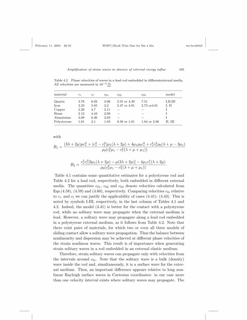
February 11, 2004 20:10 WSPC/Book Trim Size for 9in x 6in ws-book9x6
Amplification of strain waves in absence of external energy influx 105
Table 4.2 Phase velocities of waves in a lead rod embedded in differentexternal media.All velocities are measured in 10−3 m
sec
material cτ cl c01 c02 c03 model
Quartz 3.78 6.02 2.06 2.55 or 4.39 7.51 I,II,IIIIron 3.23 5.85 2.2 2.47 or 4.91 2.73 or4.81 I, IICopper 2.26 4.7 2.11 − − IBrass 2.12 4.43 2.08 − − IAluminium 3.08 6.26 2.03 − − IPolystyrene 1.01 2.1 1.83 0.38 or 1.81 1.84 or 2.06 II, III
with
B1 =(3λ + 2µ)µc2
τ + (c2τ − c2
l )µ1(λ + 2µ) + 4µ1ρ0c4τ + c2
τ c2l ρ0(λ + µ− 3µ1)
ρ0(c2l µ1 − c2
τ (λ + µ + µ1))
B2 =c2τ c2
l [3µ1(λ + 2µ)− µ(3λ + 2µ)]− 4µ1c4τ (λ + 2µ)
ρ0(c2l µ1 − c2
τ (λ + µ + µ1)).
Table 4.1 contains some quantitative estimates for a polystyrene rod andTable 4.2 for a lead rod, respectively, both embedded in different externalmedia. The quantities c01, c02 and c03 denote velocities calculated fromEqs.(4.58), (4.59) and (4.60), respectively. Comparing velocities c0i relativeto cτ and cl we can justify the applicability of cases (4.41)- (4.43). This isnoted by symbols I-III, respectively, in the last column of Tables 4.1 and4.2. Indeed, the model (4.41) is better for the contact with a polystyrenerod, while no solitary wave may propagate when the external medium islead. However, a solitary wave may propagate along a lead rod embeddedin a polystyrene external medium, as it follows from Table 4.2. Note thatthere exist pairs of materials, for which two or even all three models ofsliding contact allow a solitary wave propagation. Thus the balance betweennonlinearity and dispersion may be achieved at different phase velocities ofthe strain nonlinear waves. This result is of importance when generatingstrain solitary waves in a rod embedded in an external elastic medium.
Therefore, strain solitary waves can propagate only with velocities fromthe intervals around c0i. Note that the solitary wave is a bulk (density)wave inside the rod and, simultaneously, it is a surface wave for the exter-nal medium. Then, an important difference appears relative to long non-linear Rayleigh surface waves in Cartesian coordinates: in our case morethan one velocity interval exists where solitary waves may propagate. The

February 11, 2004 20:10 WSPC/Book Trim Size for 9in x 6in ws-book9x6
106 Amplification of Nonlinear Strain Waves in Solids
main difference between modes lies in the different rate of wave decay inthe external medium, that follows from the different behavior of Bessel’sfunctions at large values of their arguments.
Now let us consider the influence of the type of external medium onthe existence of either compression or tensile longitudinal strain localizedwaves. Using the data from Table 4.1 to compute the value of A (4.55) fora polystyrene rod, it yields that its sign may change according to the valuesof the parameters of the material used for the external medium. Thereforethe solitary wave (strain!) amplitude (4.54) may change its sign. Theamplitude is negative for a free lateral surface rod and it remains negativeif the external medium is, say, quartz, brass, copper or iron. However, thesign changes if c0 = c02 and the external medium is aluminium. Therefore,one can anticipate, in particular, that for a rod embedded in aluminiuman initial pulse with velocity close to c02 may transform only into a tensilesolitary wave while an initial pulse with velocity close to c01 evolves tobecome a compression solitary wave.
Finally, let us consider the influence on the sign of c1(4.57). For case I,b11 = 0, hence the sign is defined by the sign of the quantity (b10b2 +b3)/b4.For polystyrene it is, generally, negative for all the external media in Table4.1, while for a free lateral surface it is positive. Thus, the velocity, c, ofa nonlinear wave in a rod embedded in an external medium is lower thanthe linear wave velocity, c0, while for a free surface rod nonlinear wavespropagate faster than linear waves. On the other hand, the nonlinear wavevelocity, c, in a polystyrene rod embedded in external medium is higher thanthe linear wave velocity for a rod with free lateral surface, c∗ =
√E/ρ0.
4.2.6 Numerical simulation of unsteady strain wave prop-
agation
Numerical simulation of unsteady nonlinear wave processes in elastic rodswith free lateral surface shows that for A < 0 only initial compressionpulses provide a solitary wave (4.54) or a wave train, while tensile initialpulses do not become localized and are destroyed by dispersion. On thecontrary, for A > 0 only tensile strain solitary waves may appear, seeFigs. 3.2, 3.3 , and initial compression pulses are destroyed like in Fig. 3.4.Let us consider now the case when the rod lateral surface is partly free alongthe axis and the other part is subjected to a sliding contact with an externalelastic medium, as it is shown in Fig. 4.5. Then the nonlinear strain wavepropagation is described in each part by its own equation (4.52). Matching

February 11, 2004 20:10 WSPC/Book Trim Size for 9in x 6in ws-book9x6
Amplification of strain waves in absence of external energy influx 107
Fig. 4.5 Cylindrical rod partly embedded into an external elastic medium with sliding.
is provided by the continuity of strains and its derivatives. Assume thatfor the free surface part ( k1 = 0, k2 = 0) A = A1, m = m1, while forthe embedded one, A = A2, m = m2. Let the initial solitary wave (4.54)moves from left to right in Fig. 4.5 far from the embedded part, which issupposed to be undeformed at the initial time. It was found in Samsonov(1988) that the mass M conservation in the form
d
dtM = 0, M =
∞∫
−∞v dx (4.61)
is satisfied by equation (4.52). Then using Eqs.(4.54) and (4.55) we get forthe mass M1
M1 = 2 A1 m1, (4.62)
The wave evolution along the embedded part, depends on the ratiobetween A1 and A2. Similar to the unsteady processes inside a rod withthe free lateral surface, see Sec. 3.2, an initial strain solitary wave will bedestroyed in the embedded part, if sgnA2 differs from sgnA1. Otherwiseanother solitary wave or a wave train will appear. When the initial pulse is

February 11, 2004 20:10 WSPC/Book Trim Size for 9in x 6in ws-book9x6
108 Amplification of Nonlinear Strain Waves in Solids
Fig. 4.6 Amplification and reconstruction of a strain solitary wave.
not massive enough one can see in Fig. 3.2, that only one new solitary waveappears but there is an oscillatory decaying tail. However, the contributionof the tail to the mass M is negligibly small relative to the solitary wavecontribution, hence
M2 = 2 A2 m2. (4.63)

February 11, 2004 20:10 WSPC/Book Trim Size for 9in x 6in ws-book9x6
Amplification of strain waves in absence of external energy influx 109
Comparing M1 and M2, according to Eq.(4.61) it follows
A1 m1 = A2 m2. (4.64)
Fig. 4.7 Attenuation and reconstruction of a strain solitary wave.
Therefore, if A2 < A1 the amplitude of the solitary wave increases whileits width, proportional to m−1, decreases, hence there is focusing of the soli-tary wave. On the contrary, when A2 > A1 attenuation of the solitary wave

February 11, 2004 20:10 WSPC/Book Trim Size for 9in x 6in ws-book9x6
110 Amplification of Nonlinear Strain Waves in Solids
is provided by the simultaneous decrease of the amplitude and the increaseof the wave width. Numerical simulations confirm our theoretical estimates.
Fig. 4.8 Delocalization and reconstruction of a strain solitary wave.
In Fig. 4.6 the evolution of a strain tensile solitary wave is shown in a rod,having a central part embedded in an external medium. The value of A
in the central part II, A2, is positive but smaller than the value of A1 inthe surrounding free lateral surface parts I and III, A1 > A2 > 0. In the

February 11, 2004 20:10 WSPC/Book Trim Size for 9in x 6in ws-book9x6
Amplification of strain waves in absence of external energy influx 111
embedded part II (Fig. 4.6(b)) the solitary wave amplitude exceeds the am-plitude of the initial solitary wave in Fig. 4.6(a), while its width becomesnarrower than that of the initial wave. Therefore an increase in amplitudeof the elastic strain solitary wave is possible even in an uniformly elasticrod. This may overtake the yield point inside the elastically deformed rod,hence the possible appearance of cracks or plasticity zones. In our casethe deformations of the wave front and rear are equal. Hence, the solitarywave remains symmetric on amplification at variance with the strain soli-tary wave amplification in a rod with diminishing cross section. Moreover,a plateau develops in the tail of the solitary wave in geometrically inhomo-geneous rod. These differences could be caused by the absence of mass (andenergy) conservation for strain solitary waves in a narrowing (expanding)rod.
In the case treated here, the solitary wave does not loose mass, M , henceits original shape is recovered when traversing part III in Fig. 4.6(c,d). Onecan see that an oscillatory tail of the solitary wave in Fig. 4.6(d) is lesspronounced than the tail in Fig. 4.6(c), in agreement with (4.64). Againthere is no solitary wave selection since the parameters of the recoveredwave depends upon that of the original one.
When A2 > A1 > 0, an initial tensile strain solitary wave, Fig. 4.7(a), isdrastically attenuated as soon as it enters the embedded area, Fig. 4.7(b),and its amplitude decreases while its width becomes larger. Again boththe reconstruction of the initial wave profile and the damping of its tailare observed in the third part of a rod with free lateral surface, part III inFig. 4.7(c,d).
Consider now the case of different signs of Ai and assume that A1 > 0on both free surface parts. One can see in Fig.4.8 how an initial tensilesolitary wave, Fig. 4.8(a), is destroyed in the embedded part II, Fig. 4.8(b),in agreement with our previous results on the unsteady processes occurringfor a free surface rod. However, a strain wave is localized again in the thirdpart of a rod with free lateral surface, Fig. 4.8(c), part III , and finallyrecovers its initial shape in Fig. 4.8(d). Again damping of the tail behindthe solitary wave is observed. Accordingly, both compression and tensileinitial pulses may produce localized strain solitary waves in a rod partlyembedded in an external elastic medium with sliding.
Moreover, the amplitude of the solitary wave generated in such a man-ner, may be greater than the magnitude of the initial pulse. This case isshown in Figs. 4.9, 4.10 where A1 < 0, A2 > 0 and |A1| < A2. One can seein Fig. 4.9 how an initially localized rectangular tensile pulse, Fig. 4.9(a), is

February 11, 2004 20:10 WSPC/Book Trim Size for 9in x 6in ws-book9x6
112 Amplification of Nonlinear Strain Waves in Solids
Fig. 4.9 Generation of a tensile strain solitary wave train in a rod. The elastic propertiesof the rod are chosen such that tensile wave propagation cannot occur in the absence ofcontact with an external medium.
destroyed in the free surface part I, Fig.4.9(b). However, a wave train of soli-tary waves appears, when a destroyed strain wave comes to the embeddedpart, Figs. 4.9(c,d). The amplitude of the first solitary wave in Fig. 4.9(d)exceeds the magnitude of the initial rectangular pulse in Fig. 4.9(a). Inthe absence of surrounding external medium this rod wave-guide does not

February 11, 2004 20:10 WSPC/Book Trim Size for 9in x 6in ws-book9x6
Amplification of strain waves in absence of external energy influx 113
Fig. 4.10 Delocalization of a strain solitary wave in the absence of external medium.
support tensile solitary wave propagation, and a strain wave is delocalizedas shown in Fig. 4.10.
February 11, 2004 20:10 WSPC/Book Trim Size for 9in x 6in ws-book9x6
114 Amplification of Nonlinear Strain Waves in Solids
4.3 Strain solitary waves in an elastic rod with microstruc-ture
Classic elastic theory cannot account for phenomena caused by the mi-crostructure of a material. A particular case is a dispersion of strain wavesin an elastic medium. The influence of microstructure may provide dissipa-tive effects Cermelli and Pastrone (1997); Engelbrecht and Braun (1998);Maugin and Muschik (1994), it will be studied in Chapter 6, now consid-eration is restricted by the non-dissipative case.
The present section refers to the study of nonlinear solitary waves insidecylindrical rod with microstructure following Porubov (2000). The problemis solved using the ”pseudo-continuum” Cosserat model and the Le Rouxcontinuum model. A procedure is developed for derivation of the modelequation for long longitudinal strain waves inside the rod. The influenceof the microstructure on the solitary wave propagation and amplification isstudied.
4.3.1 Modelling of non-dissipative elastic medium with mi-
crostructure
The theory of microstructure has been developed recently, see Engel-brecht and Braun (1998); Eringen (1968); Mindlin (1964); Nowacki (1975);Nowacki (1986a) and references therein. Most of results belong to the lineartheory of elasticity, however, there are findings in the field of the nonlineartheory Engelbrecht and Braun (1998); Eringen (1968). Strain waves werestudied mainly in the linear approximation Eringen (1968); Mindlin (1964);Nowacki (1975); Nowacki (1986a). Only a few works are devoted to thenonlinear waves in microstructured non-dissipative media Engelbrecht andBraun (1998); Erbay et. al (1991); Erofeev and Potapov (1993); Erofeev(2002); Savin et. al (1973a); Savin et. al (1973b). Waves in elastic waveguides with microstructure were out of considerable investigation. Alsothe values of the parameters characterizing microstructure, are unknownas a rule, only a few experiments may be mentioned, Savin et. al (1973b);Potapov and Rodyushkin (2001).
Recall some basic ideas following Eringen (1968). Suppose the macroele-ment of an elastic body contains discrete micromaterial elements. At anytime the position of a material point of the αth microelement may be

February 11, 2004 20:10 WSPC/Book Trim Size for 9in x 6in ws-book9x6
Amplification of strain waves in absence of external energy influx 115
expressed as
x(α) = x + ξ(α),
where x is the position vector of the center of mass of the macroelement,ξ(α) is the position of a point in the microelement relative to the center ofmass. The motion of the center of mass depends upon the initial positionX and time t, x = x(X, t), while for ξ(α) the axiom of affine motion isassumed,
ξ(α) = χK(X, t) Ξ(α)K ,
where Ξ(α) characterizes initial position of a point relative to the centerof mass. Then the square of the arc length is (ds(α))2 = dx(α)dx(α), andthe difference between the squares of arc length in the deformed and unde-formed body is
(ds(α))2 − (dS(α))2 = (xk,K xk,L − δKL + 2xk,K χkM,L ΞM +
χkM,K χkN,L ΞM ΞN )dXK dXL +
2 (xk,K χkL − δKL + χkL χkM ΞM ) dXK dΞL +
χkK χkLdΞK dΞL. (4.65)
where δKL is the Kronecker delta. Let us introduce vector of macrodis-placements, U(X, t) and tensor of microdisplacements, Φ(X, t),
xk,K = (δLK + UL,K)δkL,
χkK = (δLK + ΦLK)δkL
Then three tensors characterizing the behavior of microstructuredmedium follow from (4.65),
CKL =12
(UK,L + UL,K + UM,KUM,L) ,
EKL = ΦKL + UL,K + UM,K ΦML,
ΓKLM = ΦKL,M + UN,K ΦNL,M ,
where CKL is the Cauchy-Green macrostrain tensor , EKL is the tensorof a reference distortion, ΓKLM is the tensor of microdistortion. Tensor ofthe second rank EKL accounts for the microelements motion relative to thecenter of mass of the macroelement, while tensor of the third rank ΓKLM
characterizes relative motion of the microelements of one another.

February 11, 2004 20:10 WSPC/Book Trim Size for 9in x 6in ws-book9x6
116 Amplification of Nonlinear Strain Waves in Solids
The density of the potential energy Π should be the function of thesetensors, Π = Π(CKL, EKL, ΓKLM ), more precisely upon the invariants ofthem. The bulk density of the kinetic energy has the form Mindlin (1964)
K =12ρ0
(U2
M,t + JKN ΦKM,t ΦNM,t
), (4.66)
where ρ0 is macrodensity of the elastic material, JKN is the inertia tensor.Elastic media with central symmetry posses simpler representation, JKN =J∗δKN .
One of the main problem is to define integrity basis of three tensorsCKL, EKL,ΓKLM Spencer (1971); Eringen and Suhubi (1964). Moreover,the basic invariants of the third and higher rank tensors have not beenstudied. That is why the models were developed based on the additionalassumption on a relationship between U and Φ. One of them is the pseudo-continuum Cosserat model . According to it
ΦKL = −εKLMΦM , ΦM =12εMLKUK,L, (4.67)
where εKLM is the alternating tensor. The first relationship representsthe classic Cosserat model when only rotations of solid microelements arepossible. The last expression in (4.67) accounts for the pseudo-continuumCosserat model when micro-rotation vector Φ coincides with the macro-rotation vector. In this case the density of the potential energy my beeither Π = Π(CKL, ΓKLM ) or Π = Π(CKL,ΦK,L) Nowacki (1975); Nowacki(1986a); Savin et. al (1973b). Tensor EKL has the form
EKL =12
(UK,L + UL,K + UM,KUM,L − UM,KUL,M ) ,
and only linear part of EKL coincides with those of CKL. Assume the mi-crostructure is sufficiently weak to be considered in the linear approximationNowacki (1975); Nowacki (1986a); Savin et. al (1973b), and the Murnaghanmodel is valid for the macro-motion. Then the density of the potential en-ergy may be written as
Π =λ + 2µ
2I21 − 2µI2 +
l + 2m
3I31 − 2mI1I2 + nI3 + 2µM2(ΦK,LΦK,L +
ηΦK,LΦL,K + βΦK,KΦL,L), (4.68)
where λ and µ are the Lame coefficients, (l, m, n) are the third order elasticmoduli, or the Murnaghan moduli, M , η and β are the microstructureconstants, Ip, p = 1, 2, 3 are the invariants of the tensor C, see Eq.(3.2).

February 11, 2004 20:10 WSPC/Book Trim Size for 9in x 6in ws-book9x6
Amplification of strain waves in absence of external energy influx 117
Another simplified microstructure model was used by some authors, seeErofeev and Potapov (1993); Mindlin (1964); Savin et. al (1973a). Some-times it is referred to as the Le Roux continuum Erofeev (2002). Accordingto it
ΦKL = −UL,K , ΓKLM = −UL,KM .
When microstructure is weak and may be considered in the linear ap-proximation the linear part of EKL is zero tensor. It means that thereis no difference between deformation of elastic microelement and elasticmacrostructure. In this case Π = Π(CKL,ΓKLM ). Assume again the Mur-naghan model for the macro part of the energy density and use the linearMindlin’s model Mindlin (1964) for its micro part one can obtain
Π =λ + 2µ
2I21 − 2µI2 +
l + 2m
3I31 − 2mI1I2 + nI3 + a1ΓKKMΓMLL +
a2ΓKLLΓKMM + a3ΓKKMΓLLM + a4Γ2KLM + a5ΓKLMΓMLK .
(4.69)
where ai, i = 1− 5, are the constant microstructure parameters.
4.3.2 Nonlinear waves in a rod with pseudo-continuum
Cosserat microstructure
Let us consider the propagation of a longitudinal strain wave in an isotropiccylindrical compressible nonlinearly elastic rod, see Fig. 3.1. We take cylin-drical Lagrangian coordinates (x, r, ϕ) where x is directed along the axis ofthe rod, −∞ < x <∞; r is the coordinate along the rod radius, 0 ≤ r ≤ R;ϕ is a polar angle, ϕ ε[0, 2π]. Neglecting torsions the displacement vectoris U = (u, w, 0). Then nonzero components of the macrostrain tensor Care
Cxx = ux +12(u2
x + w2x), Crr = wr +
12(u2
r + w2r), Cϕϕ =
w
r+
w2
2r2,
Crx = Cxr =12
(ur + wx + uxur + wxwr) . (4.70)
while nonzero components of the rotation tensor ΦK,L are
Φϕ,x = wxx − urx,Φϕ,r = wxr − urr. (4.71)
The governing equations together with the boundary conditions areobtained using the Hamilton variation principle (3.5), where the Lagrangian

February 11, 2004 20:10 WSPC/Book Trim Size for 9in x 6in ws-book9x6
118 Amplification of Nonlinear Strain Waves in Solids
density per unit volume, L=K − Π, with K and Π defined by Eqs.(4.66)(4.68) correspondingly.
The following boundary conditions (b.c.) are imposed:
w → 0, at r → 0, (4.72)
Prr = 0 , at r = R, (4.73)
Prx = 0, at r = R, (4.74)
where the components Prr, Prx of the modified Piola - Kirchhoff stresstensor P are defined from (3.5) with (4.66), (4.68), (4.70) and (4.71) beingtaken into account:
Prr = (λ + 2µ) wr + λw
r+ λ ux +
λ + 2µ + m
2u2
r + (λ + 2l) wrw
r+
λ + 2l
2w2
r2+ (λ + 2l) uxwr + (2l − 2m + n) ux
w
r+
λ + 2l
2u2
x +λ + 2µ + m
2w2
x + (µ + m) urwx +
3λ + 6µ + 2l + 4m
2w2
r + 4µM2(urrx − wxxr), (4.75)
Prx = µ (ur + wx) + (λ + 2µ + m) urwr + (2λ + 2m− n) urw
2r+
(λ + 2µ + m) uxur +2m− n
2wx
w
r+ (µ + m) wxwr +
(µ + m) uxwx + 4µM2[wxxx − uxxr +1r
(r(wxr − urr))r −12J∗(urtt − wxtt)]. (4.76)
Exception of torsions provides transformation of the initial 3D probleminto a 2D one. Subsequent simplification is caused by the consideration ofonly long elastic waves with the ratio between the rod radius R and typicalwavelength L is R/L ¿ 1. The typical elastic strain magnitude B is alsosmall, B ¿ 1. Then the procedure from Sec. 3.2.2 is applied to find therelationships between displacement vector components satisfying b.c. onthe lateral surface of the rod (4.73), (4.74) as well as the condition for w
(4.72). An additional parameter γ = M2/R2 is introduced to characterizethe microstructure contribution. Accordingly, the longitudinal and sheardisplacement in dimensional form are sought in the form (3.12), (3.13).

February 11, 2004 20:10 WSPC/Book Trim Size for 9in x 6in ws-book9x6
Amplification of strain waves in absence of external energy influx 119
Substituting the linear parts uL and wL (3.12), (3.13) into the b.c. (4.72)and in the linear parts of b.c. (4.73), (4.74), and equating to zero terms atequal powers of r one obtains uk and wk. Using these results the nonlinearparts uNL, wNL are similarly obtained from the full b.c. We get
u = U(x, t) +νr2
21 + 4γ
1− 4γUxx, (4.77)
w = −νrUx − ν
2(3− 2ν)(1− 4γ)[ν + 4γ(2 + ν)] r3Uxxx −
(1 + ν)[ν
2+
(1− 2ν)E
(l(1− 2ν)2 + 2m(1 + ν)− nν
)]rU2
x , (4.78)
where ν is the Poisson ratio, E is the Young modulus. Other terms from theseries (3.12), (3.13) for i > 3 may be found in the same way, however, theyare omitted here because of no influence on the final model equation forthe strain waves. Substituting Eqs.(4.77), (4.78) into Eq.(3.5), and usingHamilton’s principle we obtain that longitudinal strains, v = Ux, obey adouble dispersive nonlinear equation:
vtt − α1 vxx − α2( v2)xx + α3 vxxtt − α4 vxxxx = 0, (4.79)
where α1 = c2∗ = E/ρ0, α2 = β/(2ρ0), β = 3E + 2l(1 − 2ν)3 + 4m(1 +
ν)2(1− 2ν) + 6nν2, α3 = ν(1− ν)R2/2,
α4 =νER2
2ρ0
1 + 4γ
1− 4γ.
Hence the microstructure affects only dispersion in Eq.(4.77). The soli-tary wave solution of Eq.(4.77) is
v =3E
β
(V 2
c2∗− 1
)cosh−2(k (x− V t)), (4.80)
where V is a free parameter while the wave number k is defined by
k2 =ρ0(V 2 − c2
∗)
2νER2(
1+4γ1−4γ − (1−ν)V 2
c2∗
) . (4.81)
Therefore the contribution of the microstructure results in the wideningof the permitted solitary wave velocities,
1 <V 2
c2∗<
11− ν
1 + 4γ
1− 4γ.

February 11, 2004 20:10 WSPC/Book Trim Size for 9in x 6in ws-book9x6
120 Amplification of Nonlinear Strain Waves in Solids
Also the characteristic width of the solitary wave proportional to 1/k
becomes larger relative to the wave width in pure elastic case, γ = 0. Weconsider γ to be rather small due to the experimental data from Savinet. al (1973b). Then the type of the solitary wave (compression/tensile) isdefined by the sign of the nonlinearity parameter β like in the case withoutmicrostructure, see Sec. 3.3.
4.3.3 Nonlinear waves in a rod with Le Roux continuum
microstructure
The procedure of obtaining the governing equations is similar to those usedin previous subsection. The nonzero components of the tensor ΓKLM are
Γxxx = −uxx, Γxxr = Γrxx = −uxr, Γxrx = −wxr,
Γxrr = Γrrx = −wxr, Γrxr = −urr, Γrrr = −wrr.
The b.c. (4.73), (4.74) are satisfied for the strain tensor components
Prr = (λ + 2µ) wr + λ(w
r+ ux) +
λ + 2µ + m
2u2
r + (λ + 2l) wrw
r+
+λ + 2l
2w2
r2+ (λ + 2l) uxwr + (2l − 2m + n) ux
w
r+
λ + 2l
2u2
x +λ + 2µ + m
2w2
x + (µ + m) urwx +
3λ + 6µ + 2l + 4m
2w2
r + 2J∗(2uxtt + wrtt)− 2a1uxxx −
2(a1 + 2a2)wxxr − 2(a1 + a2)1r
(r(wrr))r − a11r
(r(uxr))r , (4.82)
Prx = µ (ur + wx) + (λ + 2µ + m) urwr + (2λ + 2m− n) urw
2r+
(λ + 2µ + m) uxur +2m− n
2wx
w
r+ (µ + m) wxwr +
(µ + m) uxwx + 2J∗urtt − a1wxrr − 2(a1 + 2a2)uxxr −2a2
1r
(r(urr))r . (4.83)
Then the approximations for the components of the displacement vectorhave the form
u = U(x, t) +νr2
21
1−NUxx, (4.84)

February 11, 2004 20:10 WSPC/Book Trim Size for 9in x 6in ws-book9x6
Amplification of strain waves in absence of external energy influx 121
w = −νrUx − 4J∗(2− ν)(1 + ν)(1− 2ν)E(3− 2ν)R2
r3Uxtt −
ν2 − (1− 2ν)(1−N)(G(1− ν)− 2νN)2(3− 2ν)(1−N)
r3Uxxx −
(1 + ν)[ν
2+
(1− 2ν)E
(l(1− 2ν)2 + 2m(1 + ν)− nν
)]rU2
x , (4.85)
where G = 2a1/µR2, N = 2a2/µR2. Like in previous section the governingequation for longitudinal strain v = Ux is the double dispersive equation(4.79) whose coefficients are defined now as
α1 = c2∗, α2 =
β
2ρ0, α3 =
νR2
2(1−N)− ν2R2
2+ 2J∗ν(2− ν), α4 =
νc2∗R
2
2(1−N),
while the solitary wave solution has the form
v =3E
β
(V 2
c2∗− 1
)cosh−2(k (x− V t)), (4.86)
where V is a free parameter, and the wave number k is defined by
k2 =(1−N)ρ0(V 2 − c2
∗)2νER2 [c2∗ − V 2 (1− ν(1−N) + 4J∗(1−N)(2− ν)/R2)]
. (4.87)
Physically reasonable case corresponds to rather small N , N < 1. Thenthe influence of the microstructure yields an alteration of the permittedsolitary wave velocities interval,
1 <V 2
c2∗<
11− ν(1−N) + 4J∗(1−N)(2− ν)/R2
.
The widening or narrowing of the interval depends upon the relationshipbetween N and the parameter of microinertia J∗. Again the type of thesolitary wave is governed by the sign of the nonlinearity parameter β. Atthe same time the characteristic width of the solitary wave proportional to1/k turns out smaller than the wave width in a pure macroelastic case,N = 0, J∗ = 0.
4.3.4 Concluding remarks
It is to be noted that the assumption of the linear contribution of themicrostructure is correct since its nonlinear contribution, being weaker,may provide alterations only in the neglected higher-order nonlinear anddispersion terms in the governing equation both the Cosserat and the Le

February 11, 2004 20:10 WSPC/Book Trim Size for 9in x 6in ws-book9x6
122 Amplification of Nonlinear Strain Waves in Solids
Roux models. Hence we don’t need in the additional nonlinear terms inthe density of the potential energy Π thus avoiding the additional un-known parameters (like Murnaghan’s third order moduli) describing thenonlinear contribution of the microstructure Eringen and Suhubi (1964);Erofeev (2002).
The alterations of the amplitude and the wave width, caused by themicrostructure, have been found in both case under study. The importantresult is in the opposite changing of the wave width which gives a possibilityto distinguish the Cosserat and the Le Roux models in possible experiments.
The dispersion caused by the microstructure may be observed experi-mentally, and numerical data on microstructure parameters my be obtainedSavin et. al (1973b). In experiments on the solitary waves propagation, seeSec. 3.4, the amplitude and the width of the wave may be measured. There-fore expressions (4.80), (4.81) provide possible estimation of the parameterM in the pseudo-continuum Cosserat model. In case of the LeRoux contin-uum there is an extra parameter J∗, see Eqs.(4.86), (4.87), and parametersN and J∗ cannot be estimated separately.
The microstructure and the surrounding medium provide similar devi-ations in the governing double dispersive equation. Hence the analysis inSec. 4.2.6 may be used if we consider a rod only part of which contains themicrostructure. Then the amplification/attenuation (but not a selection)of the strain solitary wave occurs similar to that shown in Figs. 4.6-4.10.

February 11, 2004 20:10 WSPC/Book Trim Size for 9in x 6in ws-book9x6
Chapter 5
Influence of dissipative (active)external medium
Now we study the role played by dissipation/energy influx often present in arealistic case. Dissipative/active effects may be caused by internal featuresof the elastic material, hence, an irreversible part should be included intothe stress tensor in addition to the reversible one depending only upon thedensity of the Helmholtz energy. Accordingly, the governing equations fornonlinear strains will contain dissipative/active terms. Dissipation/energyinflux may also occur in an elastic wave guide through phenomena occurringat or through its lateral surface, and this case is considered further in thisChapter. Presence of external medium makes a problem more complicated.However, the Hamiltonian formalism described in Chapter 3 may be appliedsince a wave guide remains pure elastic, all dissipative/active factors comethrough the elementary work done by the external forces, and thereforeEq.(3.29) may be used.
5.1 Contact problems: various approaches
External medium affects the lateral surface of a wave guide through the nor-mal and tangential stresses. In some cases only normal stresses may act likein the slippage contact. Various contact problems are widely considered,see, e.g., Galin (1980); Goryacheva (1998); Goryacheva (2001); Hahnerand Spencer (1998); Johnson (1985); Kalker et. al (1997); Kerr (1964);Nikitin (1998). Both elastic and viscoelastic interactions are studied theirin the linear approximation. Main attention is paid to the static loading andto the interaction forces caused by the relative movement of the contactingbodies. Of special interest if the contact with friction Goryacheva (1998);Goryacheva (2001); Hahner and Spencer (1998); Kalker et. al (1997);Nikitin (1998); Stefanski et. al (2000) . Various generalizations of the
123
February 11, 2004 20:10 WSPC/Book Trim Size for 9in x 6in ws-book9x6
124 Amplification of Nonlinear Strain Waves in Solids
Coulomb-Amonton law (dependence on the sliding velocity and the ap-parent area of contact) are studied Elmer (1997); Goryacheva (2001);Hahner and Spencer (1998); Nikitin (1998); Poschel and Herrmann (1993);Stefanski et. al (2000). However, it was noted in Hahner and Spencer(1998); Nikitin (1998); Stefanski et. al (2000) that the classical Coulomb-Amonton approach is sufficient when the relative velocity of the slidingbodies is small.
Sometimes the problem of the interaction with an external mediummay be solved directly. It means that we formulate the equation for awave guide and the medium and impose the corresponding continuity con-ditions on the lateral surface of the wave guide. An example may be foundin Sec. 4.2 where dissipationless sliding contact with an elastic externalmedium is considered. The difficulties of elastic contact stress theory mayarise because the displacement at any point in the contact surface dependsupon the distribution of pressure throughout the whole contact Johnson(1985). In this case the solution of an integral equation for the pressureis required. Another problem arises when an external medium is not elas-tic, and its behavior cannot be described by the equations of elasticity.The difficulties mentioned above may be avoided if the response of a waveguide is more interesting then the displacements and stresses distributionin the external medium. In this case the problem reduces to a develop-ment of a relatively simple foundation models to account for an influenceof the external medium in terms of the wave guide displacements and/orstrains at the lateral surface. Variety of the foundation models are col-lected in Kerr (1964). The models are designed replacing an externalmedium with interacting spring and dissipative elements. In particular,when only springs are considered and their shear interactions are assumedthe so-called Winkler-Pasternak model holds Kerr (1964); Pasternak (1954);Winkler (1867). According to it the pressure p is expressed through theshear displacement w
p = kw −G∇2w,
where ∇2 is the Laplace operator in x and y, k and G are the constantfoundation moduli. One can see its similarity with the response of theexternal medium in case of the sliding contact, see Sec. 4.2.3. Hence foun-dation models are physically reasonable since they correspond to the resultsobtained from the contact problem solutions.
It was Kerr (1964) who developed a viscoelastic foundation model.

February 11, 2004 20:10 WSPC/Book Trim Size for 9in x 6in ws-book9x6
Influence of dissipative (active) external medium 125
Based on the results of footing load tests performed on a snow basehe proposed a viscoelastic model for the interaction between an elas-tic body and the external snow (or permafrost) medium. He assumedNewton’s law for the viscous behavior thus including a dissipative ele-ments besides springs. This model will be studied in the following twosections where its mathematical expression is presented. Now we onlymention it provides the influence on a wave guide only through the nor-mal stresses. Classic case of a dissipative action through the tangentialstresses corresponds to the dry friction contact Hahner and Spencer (1998);Nikitin (1998). Here the foundation model is proposed in Sec. 5.4 when theexternal medium affects a lateral surface of an elastic rod both by the nor-mal and the tangential stresses but dissipative (active) influence is providedby the tangential stresses.
5.2 Evolution of bell-shaped solitary waves in presence ofactive/dissipative external medium
5.2.1 Formulation of the problem
Let us consider the propagation of a longitudinal strain wave in an isotropiccylindrical elastic rod embedded in an external medium subjected to Kerr’sviscoelastic contact model. Most of results were first obtained by Porubovand Velarde (2000) 1. We take cylindrical Lagrangian coordinates (x, r, ϕ)where x is directed along the axis of the rod, −∞ < x < ∞, r is the radialcoordinate, 0 ≤ r ≤ R, ϕ is a polar angle, ϕ ε[0, 2π]. Assuming thattorsions can be neglected, then the displacement vector is ~V = (u,w, 0).According to Kerr (1964) the external medium yields a normal stress P ∗rr
on the lateral surface of the rod r = R :
P ∗rr = −k
rw − η wt + χ r2 wxxt, (5.1)
where t is a time, k is the stiffness coefficient of the medium, η is theviscocompressibility coefficient of the external medium, χ is the viscositycoefficient of the external medium. All three coefficients, k, η and χ, arepositive and constant in framework of the Kerr model, however, we considera more general case with the coefficients of either sign.
The evolution of nonlinear waves is obtained in the reference configu-ration using Hamilton’s principle Eq.(3.29)), where the Lagrangian density
1Reprinted with permission from Elsevier Science

February 11, 2004 20:10 WSPC/Book Trim Size for 9in x 6in ws-book9x6
126 Amplification of Nonlinear Strain Waves in Solids
per unit volume, L, is defined as before in the book. Again we choose Mur-naghan’s approximation (3.1) for the deformation energy. Due to (5.1) theelementary work, δA, is:
δA = 2π
∫ ∞
−∞P ∗rr δw dx . (5.2)
The boundary conditions (b.c.) are:
w → 0, at r → 0, (5.3)
Prr = P ∗rr , at r = R, (5.4)
Prx = 0, at r = R, (5.5)
where the components Prr, Prx of the Piola - Kirchhoff stress tensor Pare defined by Eqs. (3.10), (3.11).
5.2.2 Dissipation modified double dispersive equation
For the longitudinal and shear displacements inside the rod we assume that:(i) pure elastic waves have strain magnitude B << 1;(ii) a characteristic strain wave length L is greater then the rod radius
R, R/L << 1.Let us obtain the approximations satisfying b.c. (5.3)- (5.5). Accord-
ing to the procedure developed in Chapter 3 the unknown functions u, w
are expanded in a power series (3.12), (3.13). Substituting them into theboundary conditions and following the approach from Sec. 3.2 we get
u = U + a2 r2 Uxx + a3 r3 Uxxt, (5.6)
w = b1 r Ux + b2 r2 Uxt + r3 (b31 Uxxx + b32 Uxtt) +
r4 (b41 Uxxxt + b42 Uxttt) + B1 r U2x + B2 r2 Ux Uxt. (5.7)
where the explicit forms for the coefficients are given by
a2 =λ
2(2(λ + µ) + k), a3 = − λ η
3(2(λ + µ) + k)(3λ + 4µ + k),
b1 = −2 a2, b2 = −3 a3, b31 = − λa2
2(2λ + 3µ) + k,

February 11, 2004 20:10 WSPC/Book Trim Size for 9in x 6in ws-book9x6
Influence of dissipative (active) external medium 127
b32 =3η a3
2(2λ + 3µ) + k, b41 = −2χ a2 + η b31 + λa3
5λ + 8µ + k, b42 = − η b32
5λ + 8µ + k,
B1 = −2 b1(λ + 4l − 2m + n) + 8a22[3(λ + µ) + 2(2l + m)] + λ + 2l
2(2(λ + µ) + k),
B2 = −2η B1 + 12a2 a3[3(λ + µ) + 2(2l + m)]− 3 a3(λ + 4l − 2m + n)3λ + 4µ + k
.
Note that a2, b2, b42 are always positive, while a3, b1, b31, b32 are alwaysnegative, while the remaining coefficients may have either sign. Due to (3.1)we have to truncate the series (5.6), (5.7), hence, omitting nonlinear termsof order three and higher. Neglecting cubic nonlinear terms we have toneglect simultaneously the ”corresponding” higher order linear derivativeterms. It was shown in that solitary waves appear as a result of the bal-ance between nonlinearity and dispersion when B is of order (R/L)2. The”largest” of the cubic terms is rU3
x ∼ RB3 ∼ R(R/L)6. Then, the ”corre-sponding” comparable linear term is r5Uxxxxx, while quadratic terms arer3UxUxxx and r3(Uxx)2. Similar terms with spatio-temporal mixed deriva-tives are of the same order. Higher order terms may be added if terms likeI41 are taken into account, see (3.4).
Using Hamilton’s principle we obtain that longitudinal strains, v =Ux, obey a dissipation modified double dispersive nonlinear equation(DMDDE):
vtt − α1 vxx − α2 vxxt − α3( v2)xx − α4 vxxxx + α5 vxxtt−
α6 (v2)xxt − α7 vxxxxt + α8 vxxttt = 0. (5.8)
The explicit forms of the coefficients αi, i = 1, ..., 8, are
α1 =8a2
2 (2(λ + µ) + k)− 8λ a2 + λ + 2µ
ρ0, α2 =
8R η a22
ρ0,
α3 =3ρ0
[λ(
12
+ 2B1 − 2a2(1 + 4B1) + 4a22(1− 4a2)
)+
µ(1− 8a2B1 − 16a3
2
)− 4ka2B1+
l
(13− 4a2(1− 4a2 +
163
a22)
)+
23m(1− 4a2
2(3 + 4a2)) + 4na22],

February 11, 2004 20:10 WSPC/Book Trim Size for 9in x 6in ws-book9x6
128 Amplification of Nonlinear Strain Waves in Solids
α4 =R2
ρ0[(λ + 2µ− 4λa2) a2 + 4(λ− 2(2λ + 2µ + k) a2) b31] ,
α5 =R2
2ρ0[2ρ0 a2(1− 2a2)− 8λ b32 + 9(9λ + 10µ + 4k)a2
3+
16(2λ + 2µ + k)a2 b32], α6 = −8R a2 ηB1
ρ0, α7 = −8R3 a2
ρ0[η b31 + χa2] ,
α8 =4R 3 η
ρ0
[4a2 b32 + 9a2
3
].
The coefficients in Eq.(5.8) may take either sign depending upon the mate-rial properties of the rod and the values of k, η and χ. Higher order terms,( v3)xx, v6x etc., have been neglected when deriving Eq.(5.8) in accordancewith the early given arguments.
5.2.3 Exact solitary wave solutions of DMDDE
In the moving frame, θ = x−V t, we assume that v = v(θ) and obtain from(5.8) the following ODE:
(V 2−α1)v+α2 V v′−α3 v2−(α4−α5 V 2)v
′′+α6 V (v2)
′+V (α7−α8V
2)v′′′
+
P + P1θ = 0, (5.9)
where a dash,′, denotes ∂/∂θ; P and P1 are constants of integration. We
are interested in bell- shaped or kink- shaped solitary waves when v →const at | θ |→ ∞, hence, P1 = 0. It is seen that Eq.(5.9) coincideswith the ODE reduction of the DMKdV Eq.(1.13) obtained in the study oflong waves in surface tension gradient-driven flows Nekorkin and Velarde(1994); Nepomnyashchy and Velarde (1994). Its most general exact solutionexpressed in terms of the Weierstrass elliptic function has been obtained inSec. 2.1.3. Here we restrict consideration to its bell-shaped solitary wavelimit,
v = Ak2 cosh−2(k θ)−B, (5.10)
with
A =6(α6α7 − α1 α6 α8 + α2 α3 α8)
α26
, B =A
3k2 +
α2
2α6,

February 11, 2004 20:10 WSPC/Book Trim Size for 9in x 6in ws-book9x6
Influence of dissipative (active) external medium 129
V 2 = α1 − α2 α3
α6. (5.11)
provided
α6(α4α6 − α3α7) = (α1α6 − α2α3)(α5α6 − α3α8). (5.12)
Thus, the elastic features of the rod and the values of the parametersk, η and χ of the external medium determine the existence of exact bell-shaped strain wave solution (5.10) as well as the sign of its amplitude,A, hence, the propagation of either compression or tensile strain solitarywaves. The relationship (5.12) provides simultaneously a balance betweennonlinearity ( v2) and dispersion (v
′′) and another balance between nonlin-
ear active/dissipative ((v2)′) and linear active/dissipative (v
′′′) terms .
With Eqs.(5.11), (5.12) taken into account, Eq.(5.9) may be written as
(V∂
∂θ− α3
α6)(
α2v + α6 v2 +α6(α4 − α5V
2)α3
v′′ − α6 P
α3
)= 0. (5.13)
The ODE reduction of the Boussinesq (or KdV) equation appears in brack-ets. However, here the wavenumber k is not a free parameter of the solution(5.10), as it is prescribed by the behaviour as | θ |→ ∞. In particular, whena solution decaying at infinity is considered, then
k2 = − α2
4(α7 − α8 V 2), (5.14)
thus implying yet another restriction on the coefficients,
α8
(α1 − α2 α3
α6
)− α7 > 0. (5.15)
Eq. (5.8) also admits kink-type solutions of the form
v = Ak2 cosh−2(kθ) + D k tanh(kθ) + C, (5.16)
with
A =6(α7 − α8 V 2)
α6, D =
6(α3(α7 − α8 V 2)− α6(α4 − α5 V 2))5α6
,
C =V 2 − α1
2α3. (5.17)
There are two possibilities for k and V . On the one hand
k =110
∣∣∣∣α4 − α5 V 2
V (α7 − α8 V 2)− α3
α6
∣∣∣∣ , (5.18)

February 11, 2004 20:10 WSPC/Book Trim Size for 9in x 6in ws-book9x6
130 Amplification of Nonlinear Strain Waves in Solids
where V is a solution of the cubic equation,
α33α8 V 3−α6(α2
6−α33 α5)V 2− (α3
3 α7 +α2 α3 α26)V +α6(α1α
26 +α2
3 α4) = 0.
(5.19)On the other hand,
k2 =14
(6α2
3
α26
− (V 2 − α1)α6 + α2α3V
α3V (α7 − α8 V 2)
), (5.20)
where V is a solution of another cubic equation,
6α3α8 V 3 + α6α7V2 − 6α3α7 V + α4 α6 = 0. (5.21)
Therefore, we have in both cases the kink-shaped solution (5.16) withprescribed parameters. An initial prestressed state of the rod may trans-form into a different one as the wave passes. The loading or unloading ofthe rod depends upon the sign of D, hence on the elastic features of therod and on the parameter values of the external medium.
5.2.4 Bell-shaped solitary wave amplification and selection
Let us consider the case when the influence of the external medium is weak,and all coefficients of the active/dissipative terms in DMDDE (5.8) aresmall relative to the other coefficients, i.e., α2 = ε β2, α6 = ε β6, α7 = ε β7,α8 = ε β8, ε << 1. Then Eq.(5.8) may be written as
vtt − α1 vxx − α3( v2)xx − α4 vxxxx + α5 vxxtt =
ε(β2 vxxt + β6 (v2)xxt + β7 vxxxxt − β8 vxxttt
). (5.22)
We see that the left hand side of Eq.(5.22) is the double dispersiveequation. Thus at ε = 0, Eq.(5.22) admits an exact bell-shaped solitarywave solution. For nonzero ε we assume that a solution of Eq.(5.22) is afunction of the phase variable θ and the slow time T , v = v(θ, T ), with
θx = 1, θt = −V (T ), T = ε t.
Then from (5.22) we get that
(V 2 − α1)vθ − α3( v2)θ − (α4 − α5V2) vθθθ =
ε(2V [vT + α5 vθθT ] + VT [v + α5 vθθ]− V∂2
∂θ2[β2 v + β6 v2 +
(β7 − β8V2) vθθ]) + O(ε2). (5.23)

February 11, 2004 20:10 WSPC/Book Trim Size for 9in x 6in ws-book9x6
Influence of dissipative (active) external medium 131
The solution of Eq.(5.23) is sought using the method explained inSec. 2.2.2 in the form
v = v0 + εv1 + ... (5.24)
Substituting (5.24) into (5.23) in the leading order we have
(V 2 − α1)v0,θ − α3( v20)θ − (α4 − α5V
2) v0,θθθ = 0 (5.25)
The exact solitary wave solution of Eq.(5.25) has the form
v0 = A(T ) cosh−2(k(T ) θ), (5.26)
with
A =3(V 2 − α1)
2 α3, k2 =
V 2 − α1
4(α4 − α5V 2). (5.27)
Accordingly, s = V 2 may lie either inside the interval
α1 < s <α4
α5, if α4 − α1α5 > 0, (5.28)
or inα4
α5< s < α1, if α4 − α1α5 < 0. (5.29)
Only the interval (5.28) is acceptable for a free rod with positive Poissonratio. The interval (5.29) exists if the viscocompressibility coefficient isgreater than a given value, η > η∗, with
η∗ =√
ρ0(k + 3λ + 4µ)√4k + 9λ + 10µ
.
The correction v1 (5.24) obeys the inhomogeneous linear equation
(V 2 − α1)v1,θ − 2α3 (v0 v1)θ − (α4 − α5V2) v1,θθθ = F, (5.30)
where F is
F = 2V [v0,T + α5 v0,θθT ] + VT [v0 + α5 v0,θθ]−
V∂2
∂θ2
[β2 v0 + β6 v2
0 + (β7 − β8V2) v0,θθ
].
The operator M acting on the function v1 in Eq.(5.30) is adjoint to theoperator
MA = (α1 − V 2)∂θ + 2α3 v0∂θ + (α4 − α5V2) ∂3
θ .

February 11, 2004 20:10 WSPC/Book Trim Size for 9in x 6in ws-book9x6
132 Amplification of Nonlinear Strain Waves in Solids
Table 5.1 Selection of solitary wave velocity for the case α4 − α1α5 > 0.
q1 s1q s2q s0 s∗
> 0 (α1; sQ) (α4/α5;∞) (α1; sQ) s1q
> 0 (α1; s2q) (s1q ; sQ) (α1; s2q) s1q
> 0 (α1; sQ) (sQ; α4/α5) (α1; sQ) s1q
> 0 (α1; sQ) (sQ; α4/α5) (sQ; α4/α5) s2q
> 0 (sQ; s2q) (s1q ; α4/α5) (s1q ; α4/α5) s2q
> 0 (0; α1) (sQ; α4/α5) (sQ; α4/α5) s2q
< 0 (0; α1) (α1; sQ) (α1; sQ) s2q
< 0 (α1; s2q) (s1q ; sQ) (s1q ; sQ) s2q
< 0 (sQ; s2q) (s1q ; α4/α5) (sQ; s2q) s1q
< 0 (sQ; α4/α5) (α4/α5;∞) (sQ; α4/α5) s1q
Then using Eq.(5.25) one can obtain the solvability condition (2.43) forEq.(5.30),
∫ ∞
−∞v0 F dθ = 0, (5.31)
which yields the equation for the function s,
sT Q3(s) = s (s− α1)2(q1 s2 + q2 s + q3), (5.32)
with
Q3(s) = α1α4(5α4 − α1α5) + 2α4(11α1α5 − 10α4) s−
3α5(17α4 − 5α1α5) s2 − 30α25 s3, (5.33)
q1 = 12α5β6 − 5α3β8, q2 = 12β6(α4 − α1α5) + α3(7β2α5 − 5β7 + 5α1β8),(5.34)
q3 = α3(7β2α4 + 5α1β7)− 12α1α4β6.
Important features of the behavior of s may be established analyzing(5.32) without integration. Note that Q3(α1) = −15α1(α4 − α1α5)2 whileQ3(α4/α5) = α4/α5 (α4 − α1α5)2, and Q3 always changes its sign insidethe interval (α1, α4/α5) permitted for s. The most interesting evolution ofs is realized when s tends to the finite constant value s∗ as T → ∞. Thevalues of s∗ are the solutions of equation
q1 s2 + q2 s + q3 = 0. (5.35)

February 11, 2004 20:10 WSPC/Book Trim Size for 9in x 6in ws-book9x6
Influence of dissipative (active) external medium 133
First, consider the case α4 − α1α5 > 0. Then α1 < s < α4/α5, and Q3
cannot have more than one root inside the interval (5.28). Assume thatthe root of Q3 is sQ while real roots of Eq.(5.35) are s1q < s2q. We denoteby s0 the initial value of s. All possibilities of the solitary wave velocityselection are collected in Table 5.1. The most interesting case correspondsto q1 positive when s1q ∈ (α1; sQ), s2q ∈ (sQ; α4/α5). Table 5.1 shows (seethird and fourth rows) that two different solitary waves may be selecteddepending on the initial value s0. Moreover, any initially initial solitarywave with velocity s0 from the permitted interval (5.28) transforms intoa dissipative solitary wave (5.26). Here we are dealing with the selectionof a symmetric solitary wave. It occurs according to Fig. 1.17, the onlydifference is the presence of two thresholds, s1q and s2q.
When Eq.(5.35) has no multiple root, s1q = s2q = sq, s tends to s∗ = sq
at q1 > 0 if
α1 < sq < sQ, α1 < s0 < sq, or sQ < sq < α4/α5, sq < s0 < α4/α5.
For negative values of q1 we also have two possibilities
α1 < sq < sQ, α1 < s0 < sQ, or sQ < sq < α4/α5, sQ < s0 < sq.
The same analysis may be performed for the case α4−α1α5 < 0. Underconditions (5.12) the asymptotic solution (5.26) coincides with the exactsolution (5.10).
We consider here in details only the cases when the velocity tends toone or another root of Eq.(5.35). Other possibilities corresponding to theblow-up or the damping of the solitary wave (5.26) may be similarly studied.
There remains the problem of whether solitary wave selection is achievedin finite or infinite time. Eq. (5.32) may be integrated in the general casegiving the implicit dependence of s on T . In order to avoid cumbersomealgebra we consider one particular case only, α1 = 1, β2 = 1, α3 = 1, α4 =2, α5 = 1, β6 = 2, β7 = 1, β8 = 1, ε = 0.1. Then the permitted interval fors is (1, 2) , and Q3(s) has only one root, sQ = 1.588, inside this interval. Forthe roots of Eq.(5.35) we have s1q = 1.324, s2q = 1.745. Therefore, this isthe case of complete selection when all initially dissipationless solitons withinitial velocity from the interval 1 < s0 < 1.588 transform into a dissipativesolitary wave with velocity s∗ = 1.588. When 1.588 < s0 < 2 they go to adissipative solitary wave with s∗ = 1.745. Integration of Eq. (5.32) yields
exp T =∣∣∣∣s0 − s1q
s− s1q
∣∣∣∣p1
∣∣∣∣s0 − s2q
s− s2q
∣∣∣∣p2
(s− 1s0 − 1
)p3 (s0
s
)p4
exp[
p5(s− s0)(s− 1)(s0 − 1)
],

February 11, 2004 20:10 WSPC/Book Trim Size for 9in x 6in ws-book9x6
134 Amplification of Nonlinear Strain Waves in Solids
with p1 = 7.904, p2 = 0.420, p3 = 8.980, p4 = 0.657, p5 = 4.286. One cansee that s → s1q or s → s2q at T → ∞. Hence the wave amplitudes tendto A1 = 3(s1q − α1)/2 α3 or to A2 = 3(s2q − α1)/2 α3.
Of special interest is the evolution of an arbitrary initial pulse. It cannotbe described by the asymptotic solution. We already noted the similaritybetween the governing equation (5.8) and the DMKdV equation (1.13).For the last equation it was found that the single wave asymptotic solutionaccounts for a behaviour of the solitary waves generated from an arbitraryinput, see Sec. 2.3.1. Hence we can anticipate the evolution of the initiallocalized strains according to that shown in Figs. 2.4-2.6.
5.2.5 Concluding remarks
We have obtained a nonlinear equation, DMDDE (5.8), governing the evo-lution of bulk longitudinal long nonlinear strain waves in an elastic rodimmersed inside an active/ dissipative medium. There is an interestingsimilarity with the results found for free surface shear long waves in a ther-moconvective liquid layer described by a dissipation modified Korteweg-de Vries equation (DMKdV), see Christov and Velarde (1995); Garazoand Velarde (1991); Nekorkin and Velarde (1994); Velarde et. al (1995);Nepomnyashchy and Velarde (1994). Indeed, in the ”travelling wave” limitthe ODE reduction of our DMDDE (5.9) is functionally identical to the cor-responding ODE reduction of the DMKdV equation Christov and Velarde(1995); Nekorkin and Velarde (1994). Consequently, all exact travellingwave solutions for the latter equation are valid in our case. The dynamicalsystem representation of Eq.(5.9),
.v = y,.y = z,.z = −β z − α v y − ν y −G(v) + P,
with
α =2α6
α7 − α8V 2, β = − α4 − α5V
2
V (α7 − α8V 2), ν =
α2
α7 − α8V 2,
G(v) =α1 − V 2
V (α7 − α8V 2)v +
α3
V (α7 − α8V 2)v2.
coincides with the system studied by Nekorkin and Velarde (1994);Velarde et. al (1995) when P = 0. Therefore, we can transfer to the lon-

February 11, 2004 20:10 WSPC/Book Trim Size for 9in x 6in ws-book9x6
Influence of dissipative (active) external medium 135
gitudinal strain waves all the results about the existence of pulses, ”boundsolitons” and ”chaotic states” found for the DMKdV equation in Christovand Velarde (1995); Nekorkin and Velarde (1994); Velarde et. al (1995).
In order to get conservation laws for DMDDE (5.8) we have to rewriteit as
vt = −gx,
gt = α1 vx + α2 vxt + α3( v2)x + α4 vxxx − α5 vxtt+
α6 (v2)xt + α7 vxxxt − α8 vxttt.
Then the time evolution of the wave energy for the solutions vanishingat ±∞ is governed by the equation
∂
∂t
∞∫
−∞v g dx = α2
∞∫
−∞vx g xdx + α6
∞∫
−∞v2
x gx dx−
α7
∞∫
−∞vxx gxx dx + α8
∞∫
−∞vxt gxt dx. (5.36)
Thus, instead of energy conservation we have an input-output energybalance that at the steady state gives a vanishing l.h.s. Indeed, the firstterm in the right-hand side of (5.36) accounts for the energy input whileenergy output is provided by the third term. The second term in (5.36)may play a stabilizing or a destabilizing role depending on the sign ofα6. The last term in (5.36) is absent in the corresponding balance law forthe DMKdV equation Garazo and Velarde (1991); Nepomnyashchy andVelarde (1994). Here it diminishes the role of the third term in (5.36).These linear mixed derivative terms in (5.8) appear due to the influence ofthe Poisson effect on the kinetic energy density, K, and on the work, A,done by external forces. These terms decide the existence of either exactcompression or tensile solitary wave solutions. Moreover, due to Eq.(5.15)there is no exact solution decaying at |θ| → ∞ if α8 = 0. The correspondingvariation of velocity of the kink-shaped solution depends upon α8 due toEqs.(5.19), (5.21). Both the compression and tensile asymptotic solutionsoccur due to the mixed terms with the velocities from the intervals (5.28),(5.29). Finally, two sets of the selected solitary wave parameters result fromthe nonzero coefficient q1 (5.34) in the equation (5.35).

February 11, 2004 20:10 WSPC/Book Trim Size for 9in x 6in ws-book9x6
136 Amplification of Nonlinear Strain Waves in Solids
Our predictions about strain solitary wave selection may help to thepossible experimental generation of active/dissipative solitary waves in arod partly embedding in an external medium with the Kerr contact. Indeed,strain solitary waves may be effectively generated inside a rod with a freeboundary based on the analysis of the exact travelling solitary wave solutionof the governing double dispersive equation ( Eq.(5.8) with k, η and χ equalto zero). Also we have shown that the external medium, e.g., the permafrostmay be responsible for large wave amplification. Thus our results permit todelineate the yield point of the material. The domain of validity of Kerr’smodel could be estimated comparing theory with experiments.
5.3 Strain kinks in an elastic rod embedded in an ac-tive/dissipative medium
There are two main types of nonlinear solitary waves which could propa-gate keeping its shape, bell-shaped and kink-shaped solitary waves. Thebell-shaped solitary wave usually appears as a result of a balance be-tween nonlinearity and dispersion. Nonlinearity in a pure elastic rod iscaused by the finite stress values and the elastic material properties whiledispersion results from the finite transverse size of the rod. They arein balance when, for instance, the strain wave magnitude, B, and thewave length, L, are such that B = O(R2/L2) << 1, where R is therod radius. Here we address the question of whether besides bell-shapedsolitary waves also kink-shaped waves may propagate in an elastic rod.The kink-shaped localized traveling structure may be sustained by dif-ferent balances. There is a balance between cubic nonlinearity and dis-persion, e.g., resulted in the kink solution of the modified Korteweg-deVries (MKdV) equation case Ablowitz and Segur (1981). Another pos-sibility occurs when nonlinearity is balanced by dissipation (or accumu-lation), e.g., the kink solution of the Burgers equation Sachdev (1987);Whitham (1974). The inclusion of cubic nonlinearity requires to extend thewidely used so-called ”five constants” Murnaghan energy model, Eq.(3.1),to a more general ”nine constants” Murnaghan model, Eq.(3.4). In view ofa possible experimental test of our predictions we consider dissipative (ac-tive) phenomena occurring at the lateral boundary of an otherwise purelyelastic and hence non-dissipative rod in the bulk Kerr (1964). It allows usto cover both possibilities for longitudinal strain kink propagation. Thereis also interest in the analytical study of the simultaneous influence of dis-

February 11, 2004 20:10 WSPC/Book Trim Size for 9in x 6in ws-book9x6
Influence of dissipative (active) external medium 137
persion, nonlinearity and dissipation (or accumulation) on the evolution,particularly, amplification, of kinks. As we seen before, mathematically thedescription of these processes requires inclusion of derivatives of high orderin the model equation. Below we shall use the results obtained in Porubovand Velarde (2002) 2.
5.3.1 Formulation of the problem
Again we consider the propagation of a longitudinal strain wave in anisotropic cylindrical compressible elastic rod embedded in an externalmedium subjected to Kerr’s viscoelastic contact on the lateral surface ofthe rod r = R :
P ∗rr = −k
rw − η wt, (5.37)
As will be seen later, the third term in Eq.(5.1) now does nor affect thewave behavior. Again both k and η are assumed to be of either sign.
We choose nine constants Murnaghan’s approximation for the density ofthe potential energy, Eq.(3.4). Thus besides the third order elastic moduli,or the Murnaghan moduli (l, m, n) we are now dealing with the fourth ordermoduli (a1, a2, a3, a4) account also for nonlinear elastic properties of theisotropic material. Like Murnaghan’s third order moduli moduli, they canbe either positive or negative.
Otherwise the statement of the problem is similar to that of the previoussection with the exception of the components Prr, Prx of the Piola -Kirchhoff stress tensor P that are now written in framework of the nine-constants theory, Eq.(3.4),
Prr = (λ + 2µ) wr + λ (ux +w
r) +
λ + 2µ + m
2(u2
r + w2x ) +
3λ + 6µ + 2l + 4m
2w2
r + (2l − 2m + n) uxw
r+
λ + 2l
2(u2
x +w2
r2+ 2wr
w
r+ 2uxwr) + (µ + m) urwx +
(l + 4a1 + a2)(
w3
r3+
3ww2r
r+ u3
x + 3uxw2r
)+ (3m− a2)urwrwx +
2l − 2m + n + 24a1 + 10a2 + 2a3 + 4a4
2
(uxw2
r2+
u2xw
r+
2uxwwr
r
)+
2Reprinted with permission from Elsevier Science

February 11, 2004 20:10 WSPC/Book Trim Size for 9in x 6in ws-book9x6
138 Amplification of Nonlinear Strain Waves in Solids
(2l − µ + 12a1 + 4a2 + 2a4)(
u2xwr +
w2wr
r2
)+
(2m− n− 2a2 − a3 − 2a4)urwwr
2r+ 2(l + 2m + 2a1)w3
r +
(2m + µ− a2 − a4)uruxwx +4l − 2a2 − a3 − 2a4
4
(u2
rw
r+
ww2x
r
)+
2l + 5m− a2
2(u2
rwr + wrw2x
)+
2l + 2m− a2 − a4
2(u2
rux + uxw2x
),
(5.38)
Prx = µ (ur + wx) + (λ + 2µ + m) (urwr + uxur) + (2λ + 2m− n) urw
2r+
2m− n
2wx
w
r+ (µ + m) (wxwr + uxwx) +
2m + a4
4(3u2
rwx + w3x
)+
4l + 2m− n− 4µ− 2a2 − 2a3
4urw
2 +2m− n− 2a2 − 2a3
4w2wx
r2+
2m− n− 2a2 − a3 − 2a4
2
(uxwxw
r+
wrwxw
r
)+
4m + a4
4u3
r +
(2m + µ− a2 − a4)uxwrwx +4m− 4µ + 3a4
4urw
2x +
4l − 2a2 − a3 − 2a4
2
(uxurw
r+
urwrw
r
)+ (2l + 2m− a2 − a4)uxurwr +
2l + 5m− a2
2(uru
2x + urw
2r) +
3m− a2
2(wxw2
r + u2xwx
). (5.39)
5.3.2 Combined dissipative double-dispersive equation
Besides assumptions (i), (ii) from Sec. 5.2.2, we now assume that (iii)B ∼ R/L to provide a balance between nonlinearity and dissipation (oraccumulation).
Like before we first obtain the relationships between the longitudinaland shear displacements,
u = U + q2 r2 Uxx, (5.40)
w = b1 r Ux + b2 r2 Uxt + r3 (b31 Uxxx + b32 Uxtt) +
+B1 r U2x + B2r U3
x + B3 r2 Ux Uxt. (5.41)
where the explicit forms for the coefficients are given by
q2 =λ
2(2(λ + µ) + k), b1 = −2 q2, b2 =
2 q2 η
3λ + 4µ + k,

February 11, 2004 20:10 WSPC/Book Trim Size for 9in x 6in ws-book9x6
Influence of dissipative (active) external medium 139
b31 = − λ q2
2(2λ + 3µ) + k, b32 = − η b2
2(2λ + 3µ) + k,
B1 = −2 b1(λ + 4l − 2m + n) + 2b21[3(λ + µ) + 2(2l + m)] + λ + 2l
2(2(λ + µ) + k),
B2 = − 1(2(λ + µ) + k)
B1[λ + 4l − 2m + n + 2b1(3λ + 3µ + 4l + 2m)] +
1 + 4a1 + a2 +12b1[6l − 2µ− 2m + n + 48a1 + 18a2 + 2a3 + 8a4] +
32b21[2 + 2l − 2m + n + 32a1 + 12a2 + 2a3 + 4a4] +
b31[4− µ + 4l + 4n + 32a1 + 8a2 + 2a4],
B3 = −2η B1 − b22q2 [3(λ + µ) + 2(l + m)]− (λ + 4l − 2m + n)3λ + 4µ + k
.
Note that q2, b2 are always positive, while b1, b31, b32 are always negativewhen the coefficients in (5.37) are positive (Kerr’s model), and the othercoefficients Bi, i = 1 ÷ 3, have different signs. Due to the chosen nine-constant model we have to truncate the series (5.40), (5.41), hence, omittinghigher order nonlinear terms and the ”corresponding” higher order linearderivative terms due to the assumption (iii). The ”largest” of the quarticterms is rU4
x ∼ RB4 ∼ R(R/L)4. Then, the ”corresponding” comparablelinear term is r4Uxxxx, while the cubic term is r3U2
xUxxx. Similar termswith spatio-temporal mixed derivatives are of the same order.
Substituting (5.40), (5.41) into (3.29), and using Hamilton’s principle(3.29) we obtain that longitudinal strains, v = Ux, obey a combined dissi-pative double-dispersive (CDDD) nonlinear equation:
vtt − α1 vxx − α2 vxxt − α3( v2)xx − α4 vxxxx + α5 vxxtt−
α6 (v2)xxt − α7 ( v3)xx = 0. (5.42)
The explicit forms of the coefficients αi, i = 1÷ 7, are
α1 =8q2
2 (2(λ + µ) + k)− 8λ q2 + λ + 2µ
ρ0, , α2 =
8R η q22
ρ0,
α3 =3ρ0
[λ(
12
+ 2B1 − 2q2(1 + 4B1) + 4q22(1− 4q2)
)+

February 11, 2004 20:10 WSPC/Book Trim Size for 9in x 6in ws-book9x6
140 Amplification of Nonlinear Strain Waves in Solids
µ(1− 8q2B1 − 16q3
2
)− 4kq2B1+
l
(13− 4q2(1− 4q2 +
163
q22)
)+
23m(1− 4q2
2(3 + 4q2)) + 4nq22 ],
α4 =R2
ρ0[(λ + 2µ− 4λ q2) q2 + 4b31(λ− 2(2λ + 2µ + k) q2) ] ,
α5 =R2
ρ0[ρ0 q2(1− 2q2) + 2k(b2
2 + 4q2b32) + (9λ + 10µ)b22/2− 4λ−
4q2(λ + µ)b32],
α6 = −8R q2ηB1
ρ0
α7 =4 kB2
ρ0[B1 − 4q2] +
4ρ0l[1/2 + 4q2(16q3
2 − 8q22 + 3q2 − 1) +
2B1(1− 4q2)2] + m[1− 4q22 + 8q2(B1 + 2q2
2)(1 + 2q2)] +
2nq2[q2 − 4q22 − 2B1] + λ[1/8 + 2q2
2(1 + 4q22) + B1(1 + 2B1 + 8q2
2) +
2B2(1− 4q2)] + µ[1/4 + 8q42 + 2B1(B1 − 4q2 − 4q2
2)− 8q2B2] +
a1[1− 16q2 + 96q22 − 256q3
2 + 256q42 ] + 4a2q2[16q3
2 − 24q22 + 9q2 − 1] +
4a3q22 [1− 4q2] + 16a4q
22 [1− q2]2.
All coefficients in Eq.(5.42) are always positive in framework of the Kerrmodel, with the exception of α3 and α6 and α7 that can be of different signsdepending upon the material properties of the rod.
Note that we have obtained Eq.(5.42) in dimensional form without useof the multiple scales method and hence terms of different orders may occur,simultaneously. Indeed, due to the above given assumptions, (i) and (ii), ingeneral, the last four terms in (5.42) are smaller than the others and henceare considered small perturbations to the other four terms. We shall referto this case as the weakly dispersive limit. Note that the coefficients α3,α6 and α7 depend on the third and fourth elastic moduli. In contrast tothe second order moduli (Lame coefficients) they may be of different signsLurie (1990). Accordingly, their combination in α3 may be quantitativelysmall while not so in α7, and then the terms α3( v2)xx and α7 ( v3)xx may,quantitatively, be of the same order. Then the dissipative term, α2 vxxt,α2 = O(1), will overcome the nonlinearity and drastically alter the wave

February 11, 2004 20:10 WSPC/Book Trim Size for 9in x 6in ws-book9x6
Influence of dissipative (active) external medium 141
shape before the nonlinearity comes to play. However, if the influence of theexternal medium is weak enough, k and η are small, α2 << 1, the significantbalance will be between the quadratic-cubic nonlinearities and dispersion,slightly perturbed by the influence of dissipative terms. We shall call itthe weakly dissipative limit. Therefore, the advantage of equation (5.42)is that it embraces different important cases, for which we shall below giveexact, asymptotic and numerical solutions.
5.3.3 Exact solutions
Assuming that the solution of Eq.(5.42) depends only upon the phase vari-able θ = x− c t, then in the moving frame Eq.(5.42) becomes the O.D.E.
v′′
+ β1v′+ β2v + β3v
2 + β4(v2)′+ β5v
3 = N, (5.43)
where a dash denotes differentiation with respect to θ; N is a constant, and
β1 =α2c
α5c2 − α4, β2 =
c2 − α1
α5c2 − α4, β3 =
α3
α4 − α5c2,
β4 =α6c
α5c2 − α4, β5 =
α7
α4 − α5c2.
Eq.(5.43) is a particular case of the equation (2.16) studied in Sec. 2.1.3.Among exact solutions obtained there we consider two bounded solutions:
(i) kink-shaped solitary wave solution
v = A m tanh(mθ) + B. (5.44)
with
A =β4 ±
√β2
4 − 2β5
β5, B = − β1 −Aβ3
2β4 − 3Aβ5,
m2 =(3A2β5 − 4Aβ4)(3β2β5 − β2
3) + 4β4(β2β4 − β1β3) + 3β21β5
2(1−Aβ4)(2β4 − 3Aβ5)2. (5.45)
(ii) bounded periodic solution
v =m√−β5
cn(mθ, κ) sn(m θ, κ) dn(m θ, κ)C1 + cn2(mθ, κ)
− β3
3β5. (5.46)

February 11, 2004 20:10 WSPC/Book Trim Size for 9in x 6in ws-book9x6
142 Amplification of Nonlinear Strain Waves in Solids
with
C1 =1− 2κ2 +
√κ4 − κ2 + 1
3κ2, m2 =
β2 + 3β21
4√
κ4 − κ2 + 1,
and the following restrictions on the coefficients:
β4 = −12
√−β5, β3 = 3β1
√−β5. (5.47)
The periodic wave solution (5.46) has a functional form different from boththe KdV cnoidal wave and the MKdV bounded periodic solutionAblowitzand Segur (1981). Note also that the solution (5.46) exists only for nonvanishing β4, hence only in the presence of the nonlinear dissipative termβ4(v2)
′in Eq.(5.43). Equation (5.42), or its equivalent dynamical system,
exhibits a more complicated balance between nonlinearity, dispersion and(linear and nonlinear) dissipation required for the periodic nonlinear wavethan the standard balance between nonlinearity and dispersion that sup-plies both the KdV and the MKdV periodic solutions. When κ = 1 wehave C1 = 0, and the solution (5.43) tends to the kink-shaped solution(5.44) like the MKdV periodic solution, while the KdV cnoidal wave so-lution becomes the bell-shaped or solitary wave solution in the analogouslimit, see Fig. 1.6.
The dissipationless limit of Eq.(5.43), β1 = β4 = 0, is
v′′
+ β2v + β3v2 + β5v
3 = N. (5.48)
It corresponds to the O.D.E. reduction of the combined KdV-MKdV(CKdV) equation. The CKdV equation possesses the one-parameter kinksolution (5.44) with (5.45) if β1 = β4 = 0. However, a periodic solution ofEq.(5.48), having a kink limit at κ = 1, has a form different from (5.46):
v =√
2mκ√−β5sn(m θ, κ)− β3
3β5,
with m2 = (3β2β5 − β23)/(3β5(1 + κ2)). Moreover, Eq.(5.48) has a variety
of bell-shaped solitary wave solutions.If α4÷α7 are equal to zero we get from Eq.(5.42) the O.D.E. reduction
of the Burgers equation,
α2c v′+ (c2 − α1)v − α3v
2 = N. (5.49)

February 11, 2004 20:10 WSPC/Book Trim Size for 9in x 6in ws-book9x6
Influence of dissipative (active) external medium 143
Its kink solution has the functional form like (5.44) but with
A = −α2c
α3≡ β1
β3, B =
c2 − α1
2α3≡ − β2
2β3, m− free. (5.50)
There are two free parameters, the phase velocity c and the wave numberm. If the boundary conditions are
v → h1 at θ →∞, v → h2 at θ → −∞,
then for the kink-shaped solution of Eq. (5.43)
β4 ±√
β24 − 2β5
β5m =
h1 − h2
2,
β1 −Aβ3
2β4 − 3Aβ5= −h1 + h2
2
while the Burgers model (5.49) gives
m =(h1 − h2)β3
2β1,
β2
2β3= −h1 + h2
2.
The coefficients βi depend upon the phase velocity c, and the elastic fea-tures of the material of the rod and the parameters of the external medium.Hence, for the Burgers model any pair of hj define phase velocity and thewave number, while in general for the one-parameter solution (5.44), (5.45)as well as for the MKdV kink solution the boundary conditions imply ad-ditional restrictions on the parameters of the problem.
5.3.4 Weakly dissipative (active) case
When the viscocompressibility coefficient η is small, i.e. when the externalmedium is of little influence we can take α2 = δα2, α6 = δα6, δ << 1.Then Eq.(5.42) is the perturbed combined double-dispersive equation,
vtt − α1 vxx − α3( v2)xx − α7 ( v3)xx − α4 vxxxx + α5 vxxtt =
δ(α2 vxxt + α6 (v2)xxt) (5.51)
For nonzero δ we assume that a solution of Eq.(5.51) is a function ofthe phase variable θ = x− ct , v = v(θ). Then from Eq.(5.51) we get that
(c2 − α1)vθ − α3( v2)θ − α7 ( v3)θ − (α4 − α5c2) vθθθ =
−δ c∂2
∂θ2
[α2 v + α6 v2
]+ O(δ2). (5.52)

February 11, 2004 20:10 WSPC/Book Trim Size for 9in x 6in ws-book9x6
144 Amplification of Nonlinear Strain Waves in Solids
The solution of Eq.(5.52) is sought in the form
v = v0 + δv1 + ... (5.53)
Substituting (5.53) into (5.52) in the leading order we have the O.D.E.underlying the CKdV equation,
(c2 − α1)c0,θ − α3( v20)θ − α7 ( v3
0)θ − (α4 − α5c2) v0,θθθ = 0. (5.54)
We look for a solution satisfying the boundary conditions
v0 → h±, vi → 0, i > 0, at θ → ±∞,
and with all derivatives of vi with respect to θ vanishing at infinity. For akink h+ 6= h−.
The exact kink solution of Eq.(5.54) has the form
v0 = A m tanh(mθ)− α3/(3α7), (5.55)
with
A =
√2(α5c2 − α4)
α7m, m2 =
3α1α7 − α23 − 3α7c
2
6(α4 − α5c2). (5.56)
The correction v1 (5.53) obeys the inhomogeneous linear equation
(c2 − α1)v1,θ − 2α3 (v0 v1)θ − 3α7 (v20 v1)θ − (α4 − α5c
2) v1,θθθ =
−c∂2
∂θ2
[α2 v0 + α6 v2
0
], (5.57)
whose solution satisfies the b.c. only when
3α2α7 − 2α3α6 = 0 (5.58)
and has the form
v1 =α6 m A
2(α5c2 − α4)θ v0,θ.
Numerical integration of Eq.(5.51) allows exploration of the kink evo-lution outside the range imposed by condition (5.58). Case α2 < 0, corre-sponding to dominating damping in the linearized Eq.(5.51) is depicted inFig. 5.1 while Fig. 5.2 shows the evolution when α2 > 0, hence correspond-ing to accumulation. In both figures the steepness of the wave front (i.e.m = const) and the phase velocity of the initial MKdV kink (5.55), left

February 11, 2004 20:10 WSPC/Book Trim Size for 9in x 6in ws-book9x6
Influence of dissipative (active) external medium 145
20 40 60 80 100 120 140x
-1.5
-1
-0.5
0.5
1
v
Fig. 5.1 Numerical simulation of the MKdV kink evolution with weak dissipation.
profile, remain one and the same. The influence of dissipation (accumu-lation) shows in the growth experienced by the shelves before and behindwave fronts, with more dramatic effect in the wave front. The length ofthe shelf increases like the length of the shelf behind the perturbed KdVsoliton Ablowitz and Segur (1981) but the height also increases. As a resultno quasistationary profile is possible during the evolution of the perturbedMKdV kink at variance with the result found for the bell-shaped strainsolitary wave in Porubov and Velarde (2000).
5.3.5 Weakly dispersive case
Let us now take into account all assumptions from Sec. 5.3.2 to obtainthe dimensionless form of Eq.(5.42). Assume the scale for v is B, for x
is L, and for t is L/c0 where c0 is a characteristic velocity of the wave.The small parameter of the problem is ε = B = R/L. Suppose that ourdimensionless solution v depends upon the phase variable θ = x − ct andthat c = 1 + εc1 + ε2c2 + .... Then from Eq.(5.42) we get
(c20 − α1)vθθ + ε
(2c2
0c1vθθ − α3( v2)θθ + α2c0vθθθ
)+
ε2(c20c1[2c2 + c1]vθθ + α2c0c1vθθθ+

February 11, 2004 20:10 WSPC/Book Trim Size for 9in x 6in ws-book9x6
146 Amplification of Nonlinear Strain Waves in Solids
20 40 60 80 100 120 140x
-1.5
-1
-0.5
0.5
1
v
Fig. 5.2 Numerical simulation of the MKdV kink evolution with weak accumulation
[α5c20 − α4]vθθθθ − α7 v3
θθ + α6c0v2θθθ) = O(ε3). (5.59)
with α2 = α2/R, α4 = α4/R2 , α5 = α5/R2, and α6 = α6/R. The solutionis sought in the form
v = v0 + ε v1 + .... (5.60)
The boundary conditions are the same as for the kink solution in theweakly dissipative case. In the leading order we have c0 =
√α1, while the
next order yields the equation
∂2
∂θ2
(2α1c1 v0 − α3 v2
0 + α2√
α1 v0,θ
)= 0. (5.61)
In brackets we have the O.D.E. reduction of Burgers equation whosekink-shaped solution is
v0 = −α2√
α1
α3m tanh(mθ) +
α1c1
α3, (5.62)
In the following higher order we get an inhomogeneous linear ordinary dif-ferential equation for v1(θ),
∂2
∂θ2(2α1c1 v1 − 2α3v0 v1 + α2
√α1 v1,θ) =

February 11, 2004 20:10 WSPC/Book Trim Size for 9in x 6in ws-book9x6
Influence of dissipative (active) external medium 147
[α4 − α5α1 ]v0,θθθθ + α7 v30,θθ − α6
√α1v
20,θθθ − α1c1[2c2 + c1]v0,θθ−
α2√
α1c1v0,θθθ,
whose solution, decaying at infinity, is
v1 = v0,θ [b1θ + b2Log(cosh(mθ)) + b3] , (5.63)
provided that
c2 =1
2α23c1
(α7 [3α1c
21 − α2
2m]− c21
),
where b3 = const, while bi, i = 1, 2, depend upon the coefficients ofEq.(5.59),
b1 =c1
α2α23
(α1[α2α7 − 2α3α6]− α2α
23
),
b2 =1√
α1α2α23
(2[α1α5 − α4]α2
3 + α1α2[2α3α6 − α2α7]).
We see that b1, b2 remain nonzero even when α6 = α7 = 0. The influenceof dispersion is provided by b2 only. If b2 = b3 = 0 then v may be writtenas
v = −α2√
α1
α3m tanh(m[1 + εb1]θ) +
α1c1
α3+ O(ε2). (5.64)
Then the first term in (5.63) affects the smoothness of the wave front in thesolution (5.60). Shown in Fig. 5.3(a) is the case b1 > 0, while Fig. 5.3(b)accounts for negative values of b1. The dashed line in Fig. 5.3 accounts forthe unperturbed Burgers kink (5.44), (5.50), while solution (5.64) is shownwith a solid line. Correspondingly, in Fig. 5.4 it is shown the influenceof the second term (b1 = b3 = 0) on the shape of the solution v (5.60)vs Burgers kink (dashed line) for b2 < 0 in Fig. 5.4(a) and for b2 > 0 inFig. 5.4(b). Note the asymmetric disturbance of the profile near the upperand lower states of the solution that are exchanged with the opposite signof b2. The case b1 = b2 = 0 corresponds to a constant phase shift of theunperturbed Burgers kink solution.
The features of a quasistationary asymptotic solution can be observedwhen studying the time-dependent process of the kink formation. Numeri-cal integration of Eq.(5.42) with an initial condition in the form of a Burgerskink-shaped wave (5.44), (5.50) shows that the wave attracts the profile de-scribed by the asymptotic solution even at moderate ε. The time evolution

February 11, 2004 20:10 WSPC/Book Trim Size for 9in x 6in ws-book9x6
148 Amplification of Nonlinear Strain Waves in Solids
5 10 15 20 25 30x
0.5
1
1.5
2
2.5
v b
5 10 15 20 25 30x
0.5
1
1.5
2
2.5
v a
Fig. 5.3 Smoothness of the Burgers kink profile due to the first term in the first orderasymptotic solution: (a) b1 > 0, (b) b1 < 0.
of the wave at ε = O(1) is shown in Figs. 5.5, 5.6 where the propagation ofthe undisturbed Burgers kink is shown with a dashed line; the left profilecorresponds to the initial Burgers kink. The values of the coefficients inEq.(5.42) have been chosen such that b2, is negative for Fig. 5.5 and positive

February 11, 2004 20:10 WSPC/Book Trim Size for 9in x 6in ws-book9x6
Influence of dissipative (active) external medium 149
5 10 15 20 25 30x
0.5
1
1.5
2
2.5v b
5 10 15 20 25 30x
0.5
1
1.5
2
2.5v a
Fig. 5.4 Disturbances on the Burgers kink profile due to the second term in the firstorder asymptotic solution: (a) b2 < 0, (b) b2 > 0.
for Fig. 5.6. The three most right solid line profiles show that the quasista-tionary perturbed kink-shaped waves are rather close to the correspondingasymptotic profiles shown in Figs. 5.5, 5.6. The phase velocity remains oneand the same during the whole time and practically equal to the velocity of

February 11, 2004 20:10 WSPC/Book Trim Size for 9in x 6in ws-book9x6
150 Amplification of Nonlinear Strain Waves in Solids
20 40 60 80 100 120x
0.1
0.2
0.3
v
Fig. 5.5 Numerical simulation of the Burgers kink evolution into the quasistationaryprofile in the weakly dispersive case at b2 < 0.
the initial Burgers kink. Any other initial kink different from the Burgersone, diverges even when dispersion is small.
5.3.6 Summary of results and outlook
We have shown that kinks can propagate in a compressible elastic rod, ofradius R, when the wave characteristics, amplitude and wavelength, aresuch that B ∼ R/L << 1, a cubic nonlinearity of the elastic material istaken into account and dissipation exists e.g. due to the rod being em-bedded in an external viscoelastic medium. We have found in the weaklydispersive limit how the kink-shaped wave is selected. In contrast to thebell-shaped solitary wave selection in previous section now only the wavenumber tends to a prescribed finite value, as Eq.(5.64) indicates. Otherpossibilities exist for an exact travelling wave solution (5.44) of Eq.(5.42)as well for the perturbed MKdV kink when the additional condition (5.58)is satisfied.
High order terms do not significantly alter the wave structure in theweakly dispersive case. In such circumstance Eq.(5.42) can be approxi-mated with α6 = α7 = 0 and hence without using the fourth-order elasticmoduli, ai. This is very important from the point of view of applicationbecause for most materials the values of ai are unknown. However, if dis-

February 11, 2004 20:10 WSPC/Book Trim Size for 9in x 6in ws-book9x6
Influence of dissipative (active) external medium 151
20 40 60 80 100 120x
0.1
0.2
0.3
v
Fig. 5.6 Numerical simulation of the Burgers kink evolution into the quasistationaryprofile in the weakly dispersive case at b2 > 0.
persion becomes significant those terms must be taken into considerationfor a correct description of the strain kinks. In particular they provide thenontrivial condition 3α2α7 − 2α3α6 = 0, that allows the propagation of aquasistationary perturbed kink in the weakly dissipative case.
The influence of dissipation on the balance between nonlinearity and dis-persion appears affecting wave evolution much more drastically than whatdispersion does to the Burgers nonlinearity-dissipation balance. However,we have no kink selection in the weakly dissipative (active) case when allwave parameters tend to finite values. This seems due to the absence of ”dis-sipative (active)” cubic nonlinear terms in the r.h.s. of Eq.(5.51). However,adding a term like (v3)xxt is not permitted by the assumptions in Sec. 5.3.2.Indeed, (v3)xxt and (v4)xx will be of the same order, and thus the corre-sponding ”dissipative” quartic nonlinearity demands a simultaneous quinticnonlinear term, and so on.
Exact solutions obtained account for the case when the dispersion, dis-sipation and nonlinearity are of the same order. The existence of thesesolutions require additional restrictions studied in Sec. 5.3.3. Moreover nu-merical simulations in the weakly dispersive case point to a formal validityof the results from Sec. 5.3.5 when dispersion is not small.
As a useful aspect of our analytical study is that obtaining exact and

February 11, 2004 20:10 WSPC/Book Trim Size for 9in x 6in ws-book9x6
152 Amplification of Nonlinear Strain Waves in Solids
asymptotic solutions allow reliable testing points for time-dependent nu-merical integration. Analytic solutions could be also the starting points forthe numerical search of homoclinic and heteroclinic trajectories yieldingsolutions of possibly more complicated form than those described in thisreport. On the other hand, we have shown that an external medium, e.g.,permafrost, may be responsible for the amplification of both the strain kinkand bell-shaped solitary waves, see Sec. 5.2. This may be used to locatezones of potential plasticity. In view of the lack of experimental data on thefourth order moduli our results may help in finding these moduli using thelinear algebraic relationships between them and the kink wave amplitudeand velocity obtained using B2.
Finally, note that our solutions may also be used to account for theevolution of surface waves in a heated liquid layer subjected to variationsof surface tension. Indeed, when A/H = H/L << 1, the evolution ofsurface waves with surface deformation η of amplitude A and wavelengthL in a layer of depth H is governed by the equation Porubov (1995):
ηt + γ1(η2)x + γ2ηxx + ε(γ3ηxxx + γ4(η2)xx + γ5(η3)x
)= 0, (5.65)
Eq.(5.65) describes waves past an instability threshold. Its O.D.E. reduc-tion coincides with Eq.(5.43). Note that Eq.(5.65) accounts only for theweakly dispersive case. Contrary to the elastic bulk dissipation–free rodinside the liquid layer here the dissipation is caused by fluid viscosity andheat diffusion.
5.4 Influence of external tangential stresses on strain soli-tary waves evolution in a nonlinear elastic rod
5.4.1 Formulation of the problem
Let us use the same notations as in previous sections. The elementary work,δA, done by normal and tangential external forces at the lateral surface ofthe rod, r = R, now is:
δA = 2π
∫ ∞
−∞(P ∗rr δw + P ∗rx δu)dx . (5.66)
We assume the external medium yields a normal stress P ∗rr ,
P ∗rr = −k1
rw + k2r wxx, (5.67)

February 11, 2004 20:10 WSPC/Book Trim Size for 9in x 6in ws-book9x6
Influence of dissipative (active) external medium 153
where ki are the stiffness coefficients of the external medium, both k1 andk2 are positive and constant. It corresponds to the Pasternak (1954) modelbased on the representation of the contact by means of the interactingspring elements, see also Kerr (1964) and references therein. Tangentialstresses on the lateral surface are assumed in the form:
P ∗rx = kdP∗rr, (5.68)
that relates to the Coulomb-Amonton law Hahner and Spencer (1998);Nikitin (1998) when kd > 0 is a friction coefficient. We consider a moregeneral model, kd is of either sign, in order to account for the influence ofan active external medium providing an energy influx .
Hence the boundary conditions (b.c.) are:
w → 0, at r → 0, (5.69)
Prr = P ∗rr , at r = R, (5.70)
Prx = P ∗rx , at r = R, (5.71)
where the components Prr, Prx of the Piola - Kirchhoff stress tensor Pare defined by Eqs. (3.10), (3.11).
5.4.2 Derivation of the governing equation
Simplifications follows from the natural assumptions are similar to thoseused in previous sections:
(i) pure elastic strain waves have magnitude B << 1;(ii) long elastic strain waves have a characteristic length L such that
relative to the rod radius R, R/L << 1.(iii)B ∼ R2/L2.Let us obtain the relationships between longitudinal and shear displace-
ments satisfying b.c. (5.69)- (5.71). According to the procedure developedin Sec. 3.2 the unknown functions u, w are expanded in a power series(3.12), (3.13) that yields in our case:
u = U + kd a1r Ux + a2 r2 Uxx + kd A1 r U2x , (5.72)
w = b1 r Ux + kd b2 r2 Uxx + b3r3 Uxxx + B1 r U2
x . (5.73)
where

February 11, 2004 20:10 WSPC/Book Trim Size for 9in x 6in ws-book9x6
154 Amplification of Nonlinear Strain Waves in Solids
a1 = −k1
µb1, a2 = − [µ2(3λ + 4µ + k1) + 2 k2
d k21λ ]b1
2µ2(3λ + 4µ + k1),
b1 = − λ
2(λ + µ) + k1, b2 =
k1λ b1
µ(3λ + 4µ + k1), b3 =
(k2 b1 − λa2)2(2λ + 3µ) + k1
,
A1 = −k1
µB1,
B1 = −λ + 2l + 2(λ + 4l − 2m + n)b1 + 2[3(λ + µ) + 4l + 2m]b21
2(2(λ + µ) + k1).
Note that a1, a2, are always positive, b1- b3 are always negative, whilenonlinear term coefficients A1, B1 have different but opposite signs. Due tothe chosen five-constant theory (3.1) we have to truncate the series (5.6),(5.7) like before in order to omit negligibly small higher-order nonlinearterms and the ”corresponding” higher order linear derivative terms due tothe assumption (iii).
Substituting Eqs.(5.72), (5.73) into Eq.(3.29) we obtain that longitudi-nal strains, v = Ux, obey a nonlinear dispersive-dissipative equation
vtt−α1 vxx−α2 ( v2)xx−α3 vxxtt +α4 vxxxx = kd(β1vx +β2 (v2)x +β3vxxx),(5.74)
where
α1 =λ + 2µ + 4[λ + b1(λ + µ)]b1 + 2k1 (b2 − b2
1)ρ0
+3 k2
1k2db2
1
µρ0,
β1 = −2k1b1
ρ0R, β2 = −2k1B1
ρ0R
α2 =3ρ0
[12(1 + 2b1)(1 + 2b2
1) + µ(1 + 2b3
1
)+
13l(1 + 2b3
1
)+
23m(1 + 2b1)(1− b1)2 + nb2
1 + λ + 2b1(λ + µ) + 2k1b1B1+
k21k
2db2
1
µ2
((λ +
12m)(1 + 2b1) + µ(1 + b1)− 1
4nb1 − µ
b1B1
)],

February 11, 2004 20:10 WSPC/Book Trim Size for 9in x 6in ws-book9x6
Influence of dissipative (active) external medium 155
α3 =R2
2(b2
1−2a2)+R2 k2
1k2db2
1
2µ2, β3 =
2R[k2µb1 − k1µ(a2b1 + b3)− k21k
2db1b2]
µρ0
α4 =R2
2ρ0[a24µa2−2(λ+2µ)−4b1(λ−µ)+µ b2
1−8b3λ+2b1(λ+µ)]+
2R2b1
ρ0[k2µb1 − k1b3(µ− k1)] +
R2k2d
2µ2ρ0[b2
2(9λ + 10µ)µ2+
k1b2[4µ2(a2 + 1) + 2µ(µ− 3λ)]− 4k2µb21+ k2
1b14µb3 + (λ + 2µ)b1].When kd = 0 Eq.(5.74) becomes the double dispersive equation (DDE)
accounting for nonlinear strain waves in a free lateral surface rod.
5.4.3 Symmetric strain solitary waves
Even at kd = 0 Eq.(5.74) is nonitegrable by the Inverse Scattering Trans-form method Ablowitz and Segur (1981). Hence, only particular, usuallytravelling wave, exact solutions may be obtained. There exist differentapproaches based on the assumptions of the appropriate ansatz for a solu-tions. More general solutions are found in terms of the elliptic functions seeSec. 2.1. However, up to now only localized strain waves were observed inexperiments, see Sec. 3.4, and main attention is paid here on the exact so-lutions vanishing at infinity. Assume the solution of Eq.(5.74) depends onlyupon the phase variable θ = x− c t, then in the moving frame Eq.(5.74)becomes the O.D.E.
v′′′
+ kdγ1v′′
+ γ2v′+ γ3vv
′+ kdγ4v
2 + kdγ5v = 0, (5.75)
where a dash denotes differentiation with respect to θ, and
γ1 =β3
α3c2 − α4, γ2 =
α1 − c2
α3c2 − α4, γ3 =
2α2
α3c2 − α4,
γ4 =β2
α3c2 − α4, γ5 =
β1
α3c2 − α4.
Following the procedure from Sec. 2.1. we compare the leading-orderderivative term, v
′′′, and the nonlinear term, vv
′. One can see they are in
balance when a solution has the second order pole. Hence, general periodicsolution may be expressed using either the Weierstrass elliptic function , v =a1℘(θ, g1, g2) + b1, or the Jacobian elliptic function, v = a2cn
2(pθ, κ) + b2.

February 11, 2004 20:10 WSPC/Book Trim Size for 9in x 6in ws-book9x6
156 Amplification of Nonlinear Strain Waves in Solids
Localized solitary wave solution are of interest here. Since they correspondto the limit κ → 1, one can assume the solution of the form:
v = G cosh−2(pθ). (5.76)
Substituting (5.76) into Eq.(5.75) and equating to zero coefficients atcorresponding powers of tanh(pθ) one obtains
p2 =c2 − α1
4(α3c2 − α4), G =
3(c2 − α1)2α2
, (5.77)
2γ4 = γ1γ3, γ5 = γ1γ2. (5.78)
The first of the conditions (5.78) defines the phase velocity,
c2 =α4β2 + α2β3
α3β2,
while the second one imposes a restriction on the equation coefficients,
α2α3β1 + (α4 − α1α3)β2 + α2β3 = 0.
When conditions (5.78) hold Eq. (5.75) may be rewritten as
[∂
∂θ+ kdγ1](v
′′+ γ2v +
12γ3v
2) = 0,
whose solution vanishing at infinity is obtained from the equation
v′′
+ γ2v +12γ3v
2 = 0. (5.79)
Eq. (5.79) is nothing but ODE reduction of the DDE integrated twice.Its solitary wave solution is (5.76), (5.77), while the phase velocity c remainsa free parameter. Hence the general solution (5.76), (5.77), (5.78) is sup-ported simultaneously by a balance between nonlinearity, γ3vv
′, and disper-
sion, v′′′
(like DDE’s solution), and by a balance between active/dissipativeterms, kdγ1v
′′, kdγ4v
2, kdγ5v. The last balance is realized under conditions(5.78).
The coefficients αi, βj depend on the elastic features of the materialof the rod and the parameters of the external medium. They define thesign of the wave amplitude G, hence either compression, G < 0, or tensile,G > 0, wave may propagate in the rod.
Solitary wave solution exists under specific initial condition in the formof (5.76) at t = 0. It is known that in non-dissipative case even ratherarbitrary initial pulse splits into the train of solitary waves each being

February 11, 2004 20:10 WSPC/Book Trim Size for 9in x 6in ws-book9x6
Influence of dissipative (active) external medium 157
accounted for the travelling solitary wave exact solution of the DDE, seeSec. 3.3. When dissipation/accumulation predominates it destroys initialpulse before balance between nonlinearity and dispersion become to play,and no localized waves appear.
Consider now a weakly dissipative case, kd << 1, when nonlinearity anddispersion dominate over dissipation/accumulation. Assume a solution ofEq.(5.74) depends upon the phase variable θ and the slow time T , v =v(θ, T ), with
θx = 1, θt = −c(T ), T = kd t.
Then asymptotic solution of Eq.(5.74) is sought in the form
v = v0(θ) + kdv1(θ) + ...
In the leading order we get
(c2 − α1)v0,θ − (α3c2 − α4)v0,θθθ − 2α2v0v0,θ = 0, (5.80)
whose one-parameter solution has the form of (5.76), but c now dependsupon T . At order O(kd) there is an inhomogeneous linear equation for v1,
(c2 − α1)v1,θ − (α3c2 − α4)v1,θθθ − 2α2(v0v1)θ = F, (5.81)
where
F = 2cv0,T + cT v0 − 2α3cv0,θθT − α3cT v0,θθθ + β1v0 + β2v20 + β3v
′′0 .
The operator acting on the function v1 in Eq.(5.81) is adjoint to that inEq.(5.80). We look for a solution satisfying the boundary conditions
vi → 0, i º 0, at |θ| → ∞, (5.82)
Then the Fredholm alternative,∫ ∞
−∞v0F dθ = 0, (5.83)
provides the absence of secular terms. It yields the equation defining thephase velocity c,
α2cT Q6(c) = (α1 − c2)(α3c2 − α4)(6α3β2c
4 + [5α2α3β1 −6β2(α4 + α1α3)− α2β3]c2 − 5α2α4β1 +
6α1α4β2 + α1α2β3). (5.84)

February 11, 2004 20:10 WSPC/Book Trim Size for 9in x 6in ws-book9x6
158 Amplification of Nonlinear Strain Waves in Solids
where
Q6(c) = 30α23 c6 − 3α3(11α4 + 10α1α3)c4 + 2α4(11α1α3 + 10α4)c2 −
α21α3α4 − 5α1α
24.
Eq. (5.84) may be integrated giving the dependence c on T in an implicitform. However, important features of the evolution of c may be establishedstudying the sign of cT without integration. The stationary solutions of(5.84) c1 =
√α1 and c2 =
√α4/α3 correspond to p = 0 or p → ∞ in
(5.77). Other stationary solutions are defined from the equation
6α3β2c4 + [5α2α3β1 − 6β2(α4 + α1α3)− α2β3]c2 − 5α2α4β1+
6α1α4β2 + α1α2β3 = 0. (5.85)
Due to (5.77) (α1 − c2)(α3c2 − α4) < 0, and the sign of cT depends upon
the signs of the polynomial Q6(c) and the quartic polynomial in the r.h.s.of Eq. (5.84). When cT keeps its sign as time passes possible scenarios forevolution of c are either vanishing or diverging to infinity. More interestingcase is realized when, in particular, real roots of Eq.(5.85), c∗1 < c∗2, arelocated in the interval, q1 < c∗1 < c∗2 < q2, where q1, q2 are real neighboringroots of Q6(c). If α3β2 > 0 and Q6(c) > 0 at q1 < c < q2, we have cT > 0when c∗1 < c < c∗2 and cT < 0 when q1 < c < c∗1 or c∗2 < c < q2. It meansthat if an initial velocity, c(T = 0) ≡ c0 lies in the intervals c∗1 < c0 < c∗2 orc∗2 < c < q2, the velocity c(T ) tends to the finite value cs = c∗2 at T → ∞.If Q6(c) < 0, c tends to cs = c∗1 . To put this another way, the value ofvelocity is selected according to the governing equation coefficients. Thewave amplitude G(c) is selected like velocity c according to (5.77). It wascalled in Sec. 1.3 the selection from below when c0 < cs, Fig. 1.17 (a), whilethe case c0 > cs is referred to by the selection from above, Fig. 1.17(b).We see the waves remain symmetric with respect to their maximums, theiramplitudes increase (decrease) while their widths decrease (increase).
Based on Eq. (5.84) the solution of Eq.(5.81) is
v1 =C(α1 − c2)
2α2[1− tanh(pθ)] + [C +
(α1α3 − α4)c2cT
(α1 − c2)2(α3c2 − α4)θ]v0 +
[C1 +C
2θ − (α1α3 − α4)c2cT
(α1 − c2)2(α3c2 − α4)θ2]v0,θ,
February 11, 2004 20:10 WSPC/Book Trim Size for 9in x 6in ws-book9x6
Influence of dissipative (active) external medium 159
where C1 is a constant,
C = 12p[α23β2c
8 + α3(5α2α3cT − 2α1α3β2 − 2α4β2 − α2β3)c6 +
(β2α21α
23 + 4α1α3α4 + α2
4+ α2β32α1α3 + α4 −11α2α3α4cT )c4 + (α2α4cT 2α1α3 + 5α4 −α12α4β2[α1α3 + α4] + α2β3[α1α3 + 2α4])c4 −α2
1α4(α4β2 + α2β3)]/5α2(α1 − c2)3(α3c2 − α4)
One can check that evolution of the solution v = v0(θ, T ) + kdv1(θ, T )does not significantly differ from that of the solution v = v0(θ, T ). How-ever, it does not vanish at θ → −∞, and a plateau appears behind thesolitary wave. The standard matching asymptotic procedure should beused to complete the uniformly valid asymptotic solution satisfying bound-ary conditions (5.82), see Ablowitz and Segur (1981) for details. Absenceof plateau requires additional restrictions on the equation coefficients. Notethat neither exact solitary wave solution (5.76) nor asymptotic selected soli-tary wave solution exists at β2 = 0, β3 = 0, and two values of the selectedwave parameters exist thanks to the mixed dispersion term in Eq.(5.74),when α3 6= 0.
5.4.4 Evolution of asymmetric solitary waves
Another asymptotic solution may be found when kd << 1 is considered butnow it is assumed that a solution of Eq.(5.74) is a function of the phasevariable θ and the slow coordinate X, v = v(θ, X), with
θx = P (X), θt = −1, X = kd x.
Then from (5.74) we get that
(1− α1P2)vθ − 2α2v vθ − (α3 − α4P
2) vθθθ = kd(2P [α1vX + α2 v2X+
(α3 − 2α4P2)vθθX ]+
PX [α1v+α2 v2θ+(α3−6α4P
2)vθθ]+P [β1v+β2v2+p2β3vθθ])+O(k2
d). (5.86)
The solution of Eq.(5.86) is sought in the form
v = v0(θ, X) + kdv1(θ, X) + ..., (5.87)
February 11, 2004 20:10 WSPC/Book Trim Size for 9in x 6in ws-book9x6
160 Amplification of Nonlinear Strain Waves in Solids
and satisfies boundary conditions (5.82). Substituting (5.87) into (5.86) wehave a nonlinear O.D.E. for v0 in the leading order,
(1− α1P2)v0,θ − 2α2v0 v0,θ − (α3 − α4P
2) v0,θθθ = 0. (5.88)
Its solution,
v0 =3(1− α1P
2)2α2P 2
cosh−2(pθ), p2 =1− α1P
2
4P 2(α3 − α4P 2)(5.89)
now accounts for a solitary wave with parameters varying with respect toX. Depending upon the function P (X) the solitary wave (5.89) may besymmetric or asymmetric with respect to its core (or maximum) at differentpoints in time, see Fig. 1.18. The evolution of the solitary wave may bedescribed solving the next order problem where an inhomogeneous linearequation holds,
(1− α1P2)v1,θ − 2α2(v0 v1)θ − (α3 − α4P
2) v1,θθθ = F, (5.90)
with
F = 2P [α1v0,X + α2 v20,X + (α3 − 2α4P
2)v0,θθX ] +
PX [α1v0 + α2 v20,θ + (α3 − 6α4P
2)v0,θθ] +
P [β1v0 + β2v20 + P 2β3v0,θθ].
Like in previous section the solvability condition (5.83) yields the equationfor the function s = P 2,
α2H3(s)sX = s (α1s− 1)(α3 − α4 s)(6α3β2 + [5α2α3β1−
6β2(α4 + α1α3)− α2β3]s− [5α2α4β1 − 6α1α4β2 − α1α2β3]s2), (5.91)
where
H3(s) = α1α4(α1α3 + 5α4)s3 − 2α4(11α1α3 + 10α4)s2+
3α3(5α1α3 + 17α4)s− 30α23.
Analysis of the solutions of Eq.(5.91) may be done similar to that in theprevious section. Again besides decay or an infinite growth of s one candescribe its selection (from below and from above) to the values ss obtainedfrom the equation

February 11, 2004 20:10 WSPC/Book Trim Size for 9in x 6in ws-book9x6
Influence of dissipative (active) external medium 161
-20 -10 10 20 30 40 50x
0.25
0.5
0.75
1
1.25
1.5
v
-20 -10 10 20 30 40 50x
-0.2
0.2
0.4
0.6
v
Fig. 5.7 Selection of the solitary waves governed by the solution (5.89), (5.91): (a) frombelow (b) from above.
[5α2α4β1 − 6α1α4β2 − α1α2β3]s2 − [5α2α3β1 − 6β2(α4 + α1α3)− α2β3]s−
6α3β2 = 0. (5.92)
We see that after substitution s = 1/c2 we get H3(s) = Q6(c)/c6 whileEqs. (5.92) coincides with Eq. (5.85). It means that parameters of the se-lected solitary waves (5.76) and (5.89) are the same as well as the conditionsrequired for the selection.

February 11, 2004 20:10 WSPC/Book Trim Size for 9in x 6in ws-book9x6
162 Amplification of Nonlinear Strain Waves in Solids
In Fig. 5.7 it is shown the temporal evolution of the solitary wave (5.89)whose amplitude and velocity vary according to Eq.(5.91). The parametersare chosen so as an initial profile is symmetric. We see that the initialwave increases, Fig. 5.7(a), or decreases, Fig. 5.7(b), into the asymmetricsolitary wave. However, it transforms back into the symmetric wave duringthe selection both from below and from above as shown in the last twostages in Fig. 5.7(a) and Fig. 5.7(b).
We have studied how the external tangential dissipative (active) forcesmay support an evolution of the long strain solitary waves in an elastic rod.The conditions are found analytically when the selection of the solitary waveoccurs both from below and from above. It is shown that both asymptoticsolutions predict evolution into the symmetric selected solitary waves.
Previously, it was found analytically and in experiments the formationof asymmetric strain solitary wave in a narrowing rod, see Sec. 4.1 wherethe governing equation corresponds to Eq.(5.74) with β1 = β1(x), β2 = 0,β3 = 0. In experiments only narrowing part of the rod was observed wherea conversion to an asymmetric wave occurs, and there is no solitary waveselection.

February 11, 2004 20:10 WSPC/Book Trim Size for 9in x 6in ws-book9x6
Chapter 6
Bulk active or dissipative sources ofthe amplification and selection
Now the attention is paid on the situations when active/dissipative forcesact inside a solid body. It is known that variation formulations used be-fore in the book cannot be applied in the presence of volume dissipativeeffects unless some modifications are proposed. Thus Lord Rayleigh (1945)involved so-called dissipation function describing forces which depend upontemporal derivatives of the variables. Dissipation function is included intovariation formulation through its elementary work. Another idea has beenused in Maugin (2000) to develop a variation formulation in thermoelastic-ity. New variable has been introduced, called thermacy, into the relationfor the free energy density.
Another approach is of phenomenological kind. The coupled govern-ing equations are derived in the form of a hyperbolic equation of mo-tion (or the equation with main hyperbolic part) and the equation for avariable responsible for dissipation (e.g., microdisplacement, temperatureetc.). The last equation is usually parabolic and is obtained phenomenolog-ically. This modelling is connected with the concept of internal variablesEngelbrecht and Braun (1998); Maugin (1990); Maugin (1999); Mauginand Muschik (1994). Application of the internal variables to the waveproblems may be found in Engelbrecht (1997); Engelbrecht et. al (1999);Engelbrecht and Maugin (1996); Maugin (1999). According to this theory,elastic stress or strain may be considered as observable variables in theusual sense of the word. Its behavior is described by the hyperbolic equa-tion. In order to compensate our lack of description of the internal structureof material or the heat processes, another variables are introduced calledinternal variables. They are usually governed by the equations of parabolictype (i.e., diffusive). Various phenomenologocal model for viscoelastic bi-ologocal media are discussed in Alekseev and Rybak (2002).
163

February 11, 2004 20:10 WSPC/Book Trim Size for 9in x 6in ws-book9x6
164 Amplification of Nonlinear Strain Waves in Solids
Below some active/dissipative problems are considered, namely, wavesin microstructured solids, seismic waves, waves in a medium with movingdefects, and thermoelastic waves. All processes are governed by coupleddissipative nonlinear partial differential equations. We do not consider hereviscoelastic materials describing by the integro- differential equations, seeabout it, e.g., Christensen (1971); Engelbrecht (1979).
6.1 Nonlinear bell-shaped and kink-shaped strain waves inmicrostructured solids
The classical theory of elasticity cannot account for effects caused by themicrostructure of a material. The theory of microstructures has beendeveloped recently, see Capriz (1989); Engelbrecht and Braun (1998);Eringen (1968); Maugin and Muschik (1994); Mindlin (1964) and refer-ences therein quoted. Most results belong to the linear theory of elastic-ity, however, there are findings in the field of the nonlinear theory En-gelbrecht and Braun (1998); Eringen (1968); Eringen and Suhubi (1964);Erofeev and Potapov (1993); Maugin and Muschik (1994). An impor-tant problem is the lack of data on the microstructure parameters, buta few works can be mentioned Savin et. al (1973b) where attempts to mea-sure them were done. Also experiments were performed in Potapov andRodyushkin (2001). Strain waves may be useful in developing a possiblemethod to estimate the microparameters since shape, amplitude and veloc-ity of the strain wave can carry informations about the microstructure.
Strain waves in microstructured medium were studied mainly in thelinear approximation Eringen (1968); Mindlin (1964). Only a few worksare devoted to the nonlinear waves in microstructured non-dissipative me-dia Engelbrecht and Braun (1998); Erofeev and Potapov (1993); Sillat(1999) while the influence of the dissipative microstructure on the evo-lution of non-linear waves has been discussed in Cermelli and Pastrone(1997); Engelbrecht (1997); Engelbrecht and Braun (1998); Engelbrechtand Khamidullin (1988) The influence of dissipation/accumulation maybe described by various methods, see Engelbrecht (1983) and referencestherein. Recently in a series of papers Cermelli and Pastrone (1997);Engelbrecht et. al (1999) the influence of dissipation on a shock propagationwas studied in the one dimensional case while inertia of the microstructurewas neglected into account together with the gradient of the microfield .Later numerical simulations were performed to account for the evolution of

February 11, 2004 20:10 WSPC/Book Trim Size for 9in x 6in ws-book9x6
Bulk active or dissipative sources of the amplification and selection 165
periodic waves Sillat (1999).Below we follow Porubov and Pastrone (2001). The model discussed in
Cermelli and Pastrone (1997); Engelbrecht et. al (1999) is modified includ-ing both the inertia of the microstructure and the gradient of the microfield. As a result the nonlinear PDE with dispersion and dissipative (active)terms is derived. It is shown that it is able to describe both the bell-shapedand kink-shaped longitudinal strain solitary waves. The simultaneous in-fluence of the accumulation/dissipation on the evolution is studied, and theselection of quasistationary dissipative solitary waves is found. A possibil-ity of the estimation of the microstructure parameters is proposed on thebasis of the results obtained here.
6.1.1 Modelling of a microstructured medium with dissipa-
tion/accumulation
Let us recall some basic ideas following Eringen (1968); Mindlin (1964). Themotion of a material particle is characterized by the displacement vectorwith components UJ (xJ , t). We suppose that the material particle containsdiscrete micromaterial elements whose displacements are accounted by themicrodisplacement vector with components U
′J(x
′J , t). Following Eringen
(1968); Mindlin (1964), we assume the microdisplacement depends linearlyon the microcoordinates x
′J : U
′J(x
′J , t) = x
′KψKJ (x, t). Hence the microdis-
placement gradient is given by ∂′IU
′J = ψIJ , thus avoiding dependence upon
microcoordinates. In a reference configuration, the fundamental strains aregiven by: the Cauchy-Green macrostrain tensor , CIJ , the distortion tensor,EIJ = ∂IUJ − ψIJ , and the microdisplacement gradient, ΓIJK = ∂IψJK .This kinematical model is valid for particular families of microstruc-tures only; if one needs a model to describe wider class of phenomena(solids with affine microstructures, liquid crystals, fluid with micro-bubbles,etc.), we refer to the references given in Cermelli and Pastrone (1997);Engelbrecht et. al (1999).
Let us assume the following:(i) the movement is one dimensional, all variables depend upon the coordi-nate x and the time t;(ii) the macromotion if small but finite. Then the geometrical nonlinear-ity is described by the only macrostrain CXX = Ux + 1/2U2
x , while theMurnaghan model is valid to account for the physical nonlinearity;(iii) the microstructure is sufficiently weak to be considered in the linearapproximation, EXX = Ux − ψ, ψ = ψXX , ΓXXX = ψx. Now and in the
February 11, 2004 20:10 WSPC/Book Trim Size for 9in x 6in ws-book9x6
166 Amplification of Nonlinear Strain Waves in Solids
following small lower indices denote differentiation.(iv) the external forces are negligible.
Then the one dimensional governing equations may be written as inMindlin (1964),
ρUtt = σx + τx, (6.1)
I ψtt = ηx + τ, (6.2)
where ρ is the macro-density, I characterizes micro inertia. In dissipation-less case components σeq, τeq and ηeq of the tensors σIJ , τIJ and ηIJK aredefined through the derivatives of the free energy W ,
σIJ =∂W
∂CIJ, τIJ =
∂W
∂EIJ, ηIJK =
∂W
∂ΓIJK,
which in the one dimensional limit Mindlin (1964); Murnaghan (1951) isreduced to:
σeq = (λ + 2µ)Ux + βU2x , τeq = D(Ux − ψ), ηeq = Gψx. (6.3)
Here λ, µ are the Lame coefficients, β = 3/2(λ + 2µ) + l + 2m, D andG are constant parameters. Assume the following representations in thegeneral case,
σ = σeq +AUxt+aψt, τ = τeq +BUxt+bψt, η = ηeq +FUxxt+f ψxt. (6.4)
Note that A and a, B and b, F and f have the same dimensions. Dissipationinequality imposes some restrictions on the involved parameters Cermelliand Pastrone (1997); Engelbrecht (1983); Engelbrecht et. al (1999); Mauginand Muschik (1994). The reason of our assumption may be seen consideringthe linearized case in absence of the microstructure. Then we have for σ:
σ = (λ + 2µ)Ux + AUxt,
that relates to the Voigt model, see, e.g., Bland (1960), the simplest exten-sion of the Hook law to the viscoelastic media Alekseev and Rybak (2002).Our model may be considered as a generalization of the Voigt model ofmicrostructured solids. Let us remark that the Voigt model accounts forthe influence of the dissipation only. We would like to consider a moregeneral case to account also for the energy influx to the strain wave causedby the microstructure. Hence the coefficients in Eq.(6.4) may be of differ-ent signs. Certainly, constitutive equations (6.4) are of phenomenologicalkind, since strictly speaking, they are not rigorously deduced within the

February 11, 2004 20:10 WSPC/Book Trim Size for 9in x 6in ws-book9x6
Bulk active or dissipative sources of the amplification and selection 167
general framework of Rational Continuum Mechanics, but we do not wantto go further in details here. In the following a more general constitutiveequations will be derived according the basic assumptions and methods ofContinuum Mechanics. Equation (6.4) can be seen as a particular case,obtained via proper additional assumptions.
Substituting Eqs.(6.3), (6.4) into Eqs. (6.1), (6.2) and introducing thefunctions v = Ux and ψ as unknown variables, we obtain the coupled equa-tions
ρvtt = (λ+2µ+D)vxx−Dψxx +β( v2)xx +(A+B)vxxt +(a+b)ψxxt, (6.5)
I ψtt = D(v − ψ) + Bvt + bψt + G ψxx + F vxxt + f ψxxt. (6.6)
Further simplifications follow considering only long waves with charac-teristic length L >> 1. Moreover, the macro strain v is elastic and doesnot exceed the yield point. Since the Murnaghan model is chosen, we aredealing with those elastic materials whose yield points are small, hence,the characteristic strain magnitude V is also small, V << 1. Let us in-troduce L as a scale for x, V - as a scale for v and ψ, L/c0, as a scale fort, c2
0 = (λ + 2µ)/ρ as a characteristic velocity. The microinertia term I
depends upon the square of a typical size p of a microstructure element.Then I may be rewritten as I = ρp2I∗, I∗ being dimensionless. Using di-mensional analysis, one can assume G = p2G∗, G∗ having the dimension ofstress. The influence of dissipation/accumulation may be conveniently de-scribed supposing A = dA∗, a = da∗, B = dB∗, b = db∗, F = dF ∗, f = df∗,where d has the dimension of a length. Then three positive dimensionlessparameters appear in Eqs.(6.5), (6.6):
(a) ε = V << 1 accounting for elastic strains;(b) δ = p2/L2 << 1, characterizing the ratio between the microstruc-
ture size and the wave length;(c) γ = d/L, characterizing the influence of the dissipation.
Then the dimensionless governing equations are (we keep the notations forvariables):
vtt − (1 +D
λ + 2µ)vxx +
D
λ + 2µψxx = ε
β
λ + 2µ( v2)xx+
γ
[(A∗ + B∗)c0
λ + 2µvxxt +
(a∗ + b∗)c0
λ + 2µψxxt
], (6.7)

February 11, 2004 20:10 WSPC/Book Trim Size for 9in x 6in ws-book9x6
168 Amplification of Nonlinear Strain Waves in Solids
Dψ = Dv + γc0 [B∗vt + b∗ψt] + δ [G∗ψxx − (λ + 2µ)I∗ψtt] +
γδc0 [F ∗vxxt + f∗ψxxt] . (6.8)
In absence of the microstructure, B∗, D, F ∗, G, a∗, b∗, and δ are equalto zero, the only equation for v is of the form
vtt − vxx − εβ
λ + 2µ( v2)xx − γ
(A∗ + B∗)c0
λ + 2µvxxt = 0. (6.9)
Assume dissipation is weak. If we expand the solution of Eq.(6.8) in theform :
ψ = ψ0 + γ ψ1 + δ ψ2 + γδ ψ3 + γ2ψ4 + ..., (6.10)
with
ψ0 = v, ψ1 =(B∗ + b∗)c0
Dvt, ψ2 =
G∗
Dvxx − (λ + 2µ)I∗
Dvtt,
ψ3 =[(F ∗ + f∗)D + (B∗ + 2b∗)G∗]c0
D2vxxt − (λ + 2µ)(B∗ + 2b∗)c0I
∗
D2vttt,
ψ4 =b∗(B∗ + b∗)c2
0
D2vtt. (6.11)
we obtain, by substituting (6.10), (6.11) into Eq.(6.7), the governing non-linear PDE for the macrostrain v(x, t),
vtt − vxx − εα1( v2)xx − γα2 vxxt + δ(α3 vxxxx − α4 vxxtt)+
γδ(α5 vxxxxt + α6 vxxttt) + γ2α7vxxtt = 0, (6.12)
where
α1 =β
λ + 2µ, α2 =
(A∗ + a∗)c0
λ + 2µ, α3 =
G∗
λ + 2µ, α4 = I∗,
α5 =[(F ∗ + f∗)D + (B∗ + b∗ − a∗)G∗]c0
(λ + 2µ)D,
α6 =I∗(a∗ −B∗ − b∗)c0
D, α7 =
a∗(B∗ + b∗)ρD
.
Comparing Eq.(6.12) with Eq.(6.9) we see that the inclusion of the gra-dient of microdistortion provides the dispersion vxxxx, while the inertia ofthe microstructure gives us mixed dissipation and dispersion terms. The

February 11, 2004 20:10 WSPC/Book Trim Size for 9in x 6in ws-book9x6
Bulk active or dissipative sources of the amplification and selection 169
evolution of nonlinear strain wave depends upon the ratio between param-eters ε, γ and δ. This is the reason we retain terms quadratic in theseparameters in the expansion of the solution (6.10). Sometimes they canbe considered ” negligibly small”, sometimes-not, according to the differenteffects we want to point out, as it will be explained in the following.
There are two main types of nonlinear travelling solitary waves whichcould propagate keeping its shape, bell-shaped and kink-shaped solitarywaves. The bell-shaped solitary wave usually appears as a result of abalance between nonlinearity and dispersion. The kink-shaped localizedtravelling structure may be sustained by different balances, one possibil-ity occurs when nonlinearity is balanced by dissipation (or accumulation),another case corresponds to the simultaneous balance between dispersion,nonlinearity and dissipation (or accumulation). Typical shapes of the wavesare shown in Figs. 1.1–1.5.
6.1.2 Bell-shaped solitary waves
The balance between nonlinearity and dispersion takes place when δ =O(ε). If in addition γ = 0, we have the nondissipative case governed by thedouble dispersive equation,
vtt − vxx − ε(α1( v2)xx − α3 vxxxx + α4 vxxtt) = 0. (6.13)
Its exact bell-shaped travelling solitary wave solution arises as a result ofbalance between nonlinear and dispersive terms. It satisfies the boundaryconditions
∂k
∂xkv → 0 for |x| → ∞, k = 0, 1, 2, 3, (6.14)
and takes the form (see section 3):
v =6k2(α4 c2 − α3 )
α1cosh−2(k θ), (6.15)
where θ = x− ct, c is a free parameter,
k2 =c2 − 1
4ε(α4c2 − α3). (6.16)
Hence, the solitary wave (6.15) exists when c2 > max1, α3/α4 orwhen 0 < c2 < min1, α3/α4. In the first case longitudinal tensile wavespropagate, while in the second case only compressive waves propagate.
February 11, 2004 20:10 WSPC/Book Trim Size for 9in x 6in ws-book9x6
170 Amplification of Nonlinear Strain Waves in Solids
In general, Eq.(6.12) possesses an exact travelling bell-shaped solutionvanishing at infinity Kudryashov (1988); Parkes and Duffy (1996),
v = −60ck3γδ
εα1(α5 + α6c
2) cosh−2(k (x− ct))[tanh(k (x− ct))± 1], (6.17)
where
k = ± 2γcα2
δ(α3 − α4c2),
α4 = α4 + ε2/δ α7, the phase velocity c is defined from the overdeterminedsystem of bi-quadratic equations,
(δα4 − γ2α7)c4 − [δ(α3 + α4) + 24γ2α22]c
2 + δα3 = 0,
(δα42 + 16γ2α2α6)c4 + (16γ2α2α5 − 2δα3α4)c2 + δα2
3 = 0,
hence, the exact solution (6.17) exists only for particular values of thecoefficients in such equations.
When δ = O(ε), γ << 1, Eq.(6.12) is considered as dissipation per-turbed double dispersive equation (6.13). The asymptotic solution is soughtas a function of the phase variable θ and the slow time T , v = v(θ, T ), with
θx = 1, θt = −c(T ), T = γ t.
Then from (6.12) we get that
(c2 − 1)vθ − εα1( v2)θ + ε(α3 − α4c2) vθθθ =
γ
(2c[vT − εα4 vθθT ] + cT [v − εα4 vθθ]− c
∂2
∂θ2
[α2 v − ε(α5 + α6c
2) vθθ
])+
O(γ2). (6.18)
The solution of Eq.(6.18) is sought in the form
v = v0(θ, T ) + γv1(θ, T ) + ... (6.19)
where vi, i = 0, 1, ..., satisfy boundary conditions (6.14) at |θ| → ∞. Sub-stituting (6.19) into (6.18) we have in the leading order
(c2 − α1)v0,θ − εα1( v20)θ + ε(α3 − α4c
2) v0,θθθ = 0. (6.20)

February 11, 2004 20:10 WSPC/Book Trim Size for 9in x 6in ws-book9x6
Bulk active or dissipative sources of the amplification and selection 171
The exact solitary wave solution of Eq.(6.20) has the form (6.15) withc = c(T ). The first order term v1 in the solution (6.19) obeys the inhomo-geneous linear equation
(c2 − α1)v1,θ − 2εα1 (v0 v1)θ + ε(α3 − α4c2) v1,θθθ = F, (6.21)
where F is
F = 2c[v0,T − εα4 v0,θθT ] + cT [v0 − εα4 v0,θθ]−
c∂2
∂θ2
[α2 v0 − ε(α5 + α6c
2) v0,θθ
].
The operator M acting on the function v1 in Eq.(6.21) is adjoint to theoperator
MA = (c2 − 1)∂θ − 2εα1 v0∂θ + ε(α3 − α4c2) ∂3
θ .
Then using (6.20) and boundary conditions at infinity one can obtainthe solvability condition for Eq.(6.21),
∫ ∞
−∞v0 F dθ = 0, (6.22)
which yields the equation for the function s = c2,
7ε sT Q3(s) = 2s (s− α1)2(q1 s2 + q2 s + q3), (6.23)
with
Q3(s) = 30α24 s3 +3α4(17α3 +5α4) s2 +2α3(10α3 +11α4) s−α3(α4 +5α3),
q1 = 5α6, q2 = 5α5 − 7α2α4 − 5α6, q3 = 7α2α3 − 5α5. (6.24)
Important features of the behaviour of s may be established analyzingEq.(6.23) without integration. There may be decay or infinite growth of theinitial velocity and the amplitude of the solitary wave (6.15). However, themost interesting evolution of s is realized when s (and hence the amplitudeof the solitary wave) tends to the finite constant value s∗ as T →∞. Hencethe solitary wave in microstructured solids may be also selected. Indeed,the values of s∗ are the real positive solutions of equation
q1 s2 + q2 s + q3 = 0. (6.25)

February 11, 2004 20:10 WSPC/Book Trim Size for 9in x 6in ws-book9x6
172 Amplification of Nonlinear Strain Waves in Solids
Assume real roots of Eq.(6.25) are s1q < s2q. We denote by s0 the initialvalue of s while the real root of Q3 is sQ. The sign of sT needed for s →snq depends upon the sign of Q3(s) around s = snq, the sign of q1, andthe permitted interval defined from (6.16). When sQ is the only real rootof Q3, and sQ < s1q the amplification of the solitary wave with s∗ = s1q
occurs at q1 > 0 if sQ < s0 < s1q while at q1 < 0 it amplifies by s∗ = s2q
if s1q < s0 < s2q. The attenuation of the wave to s∗ = s1q happens whenq1 > 0, s1q < s0 < s2q, in case q1 < 0 wave with initial velocity s0 > s2q
decreases to s∗ = s2q. When s1q < sQ < s2q there is no selection forq1 > 0, while for negative q1 the double selection is realized. Thus, waveswith s0 < s1q amplify up to s∗ = s1q, but waves with sQ < s0 < s2q increaseup to s∗ = s2q. Similarly, the attenuation to s∗ = s1q happens for the waveswith s1q < s0 < sQ, while the waves with s0 > s2q attenuate by s∗ = s2q.If sQ > s2q there is no double selection, the wave evolution is similar tothe case sQ < s1q. The situation when Q3 has three real roots within oroutside the interval [s1q, s2q] may be analyzed in the same manner. Thusthe stationary values of the solitary wave parameters are prescribed by theequation coefficients.
Amplification, attenuation and selection of the bell-shaped solitary wavev = v0 is shown in Fig. 1.17. One can see that the solitary wave keeps itslocalized bell-shaped form. In the case of amplification, the wave ampli-tude increases, while the width decreases; the attenuation is provided bysimultaneous decrease of the amplitude and the increase of the width. Theaddition of correction γv1 does not change significantly the profile of v = v0.It is relevant to notice that the solution (6.19) is not uniformly valid: thematching asymptotic expansions method Ablowitz and Segur (1981) shouldbe applied to complete the solution, even if it does not modify the behaviourof the wave near its core.
6.1.3 Kink-shaped solitary waves
The equation (6.12) possesses also exact travelling kink-shaped solutionKudryashov (1988); Parkes and Duffy (1996), in the form
v =3∑
i=0
A i tanhi(k θ), (6.26)
with three possible sets of parameters A i, k . There are no free parametersin the solution, and additional restrictions on the equation coefficients are

February 11, 2004 20:10 WSPC/Book Trim Size for 9in x 6in ws-book9x6
Bulk active or dissipative sources of the amplification and selection 173
needed.When dispersion is weak, i.e., ε2 < δ < ε and γ = O(ε), the nonlinearity
is balanced by the dissipation/accumulation only. Then Eq.(6.12) may berewritten as
vtt − vxx − ε(α1( v2)xx + α2 vxxt) = −δ(α3 vxxxx − α4 vxxtt)−
εδ(α5 vxxxxt + α6 vxxttt), (6.27)
whose solution is sought in the form
v = v0 + δv1 + ... (6.28)
where vi = vi(θ = x− ct) satisfies the boundary conditions
v0 → h±, vi → 0, i > 0, for θ → ±∞, (6.29)
and all derivatives of vi with respect to θ vanish at infinity. For a kinkh+ 6= h−. In the leading order the kink solution has the form
v = A m tanh(mθ) + B, (6.30)
with
A = −α2c
α1, B =
c2 − 12εα1
. (6.31)
There are two free parameters, the phase velocity c and the wave numberm which are defined from the boundary conditions,
m =(h− − h+)α1
2cα2, c2 = 1 + εα1(h+ + h−).
Next order solution v1 consists of two parts, v1 = v1d+ v1a, where dispersiveperturbation of the kink vanishing at infinity is accounted for the solution,
v1d =2(α4c
2 − α3)m2
εα1cosh−2(mθ) log sech(mθ), (6.32)
while higher order dissipative/active terms contribution is
v1a =2(α5 + α6c
2)cm3
α1cosh−2(mθ) (3 tanh(mθ)− 2mθ) . (6.33)
The alterations of the kink shape in absence of higher order dissipa-tive/active terms, α5 = α6 = 0, depend upon the sign of (α4c
2 − α3)/α1.Typical profiles of v = v0 + δv1d with v1d defined by (6.32) are shownin Fig. 6.1 for different values of α3 with other parameters values fixed:

February 11, 2004 20:10 WSPC/Book Trim Size for 9in x 6in ws-book9x6
174 Amplification of Nonlinear Strain Waves in Solids
-6 -4 -2 2 4 6x
-1
1
2
3
v e
-6 -4 -2 2 4 6x
-1
1
2
3
v c
-6 -4 -2 2 4 6x
-1
1
2
3
v d
-6 -4 -2 2 4 6x
-1
1
2
3
4v a
-6 -4 -2 2 4 6x
-1
1
2
3
v b
Fig. 6.1 Influence of weak dispersion on the shape of the kink-shaped wave. Shown bydashed line is the unperturbed kink.
α1 = 1, α2 = −1, α4 = 1, c = 1.5, m = 1.5, ε = 0.5, δ = 0.1. The ”non-symmetric” disturbances of the kink shape are seen in Fig. 6.1(a), whereα3 = −2.5; they become weaker when α3 tends to zero. In Fig. 6.1(b) thevalue is α3 = −0.5, while undisturbed kink appears in Fig. 6.1(c) whereα3 = 2.25. Then the disturbances develop on another ”side” of the kink,as shown in Figs. 6.1(d,e) with α3 = 5, 7, correspondingly, and we have themirror profile of those shown in Fig. 6.1(a, b). Fig. 6.1 shows the amplifi-cation of the kink-shaped wave since the difference between its maximumand its minimum is larger than in the undisturbed case. In contrast to thebell-shaped wave now the amplification is accompanied by the alterationof the wave profile. One can note the similarity with the profile in Fig. 1.5of the exact kink-shaped solution of DMKdV equation. In Fig. 6.2 itis shown what happens with the kink (6.30) when there is no dispersion,

February 11, 2004 20:10 WSPC/Book Trim Size for 9in x 6in ws-book9x6
Bulk active or dissipative sources of the amplification and selection 175
-6 -4 -2 2 4 6 x
-2-1
1234
v e
-6 -4 -2 2 4 6 x
-1
1
2
3
v c
-6 -4 -2 2 4 6 x
-1
1
2
3
v d
-6 -4 -2 2 4 6x
-1
1
2
3
v a
-6 -4 -2 2 4 6x
-1
1
2
3
v b
Fig. 6.2 nfluence of weak higher order dissipation on the shape of the kink-shaped wave. Shown by dashed line is the unperturbed kink.
α3 = α4 = 0. The profiles of v = v0 + δv1a with v1a defined by (6.33)correspond to α1 = 1, α2 = −1, α5 = 1.5, c = 1.5, m = 1.5, ε = 0.5,δ = 0.1. In Fig. 6.2(a) α6 = −2.5, it varies from α6 = −1.5, Fig. 6.2(b) toα6 = −0.5, Fig. 6.2(c) where there are no disturbances. We have α6 = 0.5in Fig. 6.2(d), while Fig. 6.2(e) corresponds to α6 = 2.5. Two main dis-tinctions may be mentioned in comparison with profiles shown in Fig. 6.1.First, the disturbances of the kink shape are ”symmetric” independently ofthe sign of α6. Second, there are no mirror profiles arising at distinct signsof α6.
The case δ = O(ε), γ = O(ε) corresponds to the simultaneous balancebetween nonlinearity, dispersion and dissipation/accumulation, perturbed

February 11, 2004 20:10 WSPC/Book Trim Size for 9in x 6in ws-book9x6
176 Amplification of Nonlinear Strain Waves in Solids
by the higher order dissipative/active terms,
vtt − vxx − ε[α1( v2)xx + α2 vxxt − α3 vxxxx + α4 vxxtt] =
−ε2(α5 vxxxxt + α6 vxxttt), (6.34)
The solution of Eq.(6.34) is sought in the form
v = v0 + εv1 + ε2v2... (6.35)
where boundary conditions (6.29) hold. Substituting (6.35) into (6.34)in the leading order we obtain the D’Alembert equation. Consider onlyone wave travelling to the left and assume v depends upon phase variableθ = x − ct with c = 1 + εc1 + ε2c2.... Then at order ε the ODE equationfor v0 is,
2c1v0,θ − α1( v20)θ + α2 v0,θθ + (α3 − α4) v0,θθθ = 0. (6.36)
Equation (6.36) possesses the exact kink-shaped solution Vlieg-Hultsman and Halford (1991),
v0 = A tanh(mθ)sech2(mθ) + B tanh(mθ) + C, (6.37)
with
A =3α2
2
50α1(α4 − α3), B =
3α22
25α1(α4 − α3), C =
c1
α1, m =
α2
10(α3 − α4).
It follows from (6.29) that
h+ − h− = 2B, c1 =α1
2(h+ + h−),
and the solution exists under special boundary conditions. The influence ofhigher order terms may be studied in a similar way as done for the solution(6.28).
6.1.4 Concluding remarks
We have found that various features of the microstructure provide corre-sponding terms in the governing equation (6.12). Thus inertia yields mixedderivative terms vxxtt, vxxttt , while dispersion vxxxx and higher order dissi-pative/active term vxxxxt are due to the micro-deformation gradient. Dis-persion is required for the existence of the bell-shaped solitary waves in anelastic microstructured medium. The dispersive term vxxtt determines, in

February 11, 2004 20:10 WSPC/Book Trim Size for 9in x 6in ws-book9x6
Bulk active or dissipative sources of the amplification and selection 177
particular, the existence of either exact compression or tensile solitary wavesolutions (see Eqs.(6.15), (6.16)), while the higher order dissipative/activeterm α6 vxxttt provides nonzero q1 in Eq.(6.25), namely two stationary fi-nite velocities of the solitary wave. Dispersion terms also account for thealterations in the kink-shaped wave profile, see Fig. 6.1, while higher or-der dissipative/active terms are responsible for a saturation which preventsunbounded growth of the bell-shaped solitary wave.
We see that pairs B∗, b∗ and F ∗, f∗ appear in the expressions for theequation coefficients only in combinations B∗ + b∗, F ∗ + f∗. Hence, onecould reduce the number of the microstructure parameters in the model(6.4). At the same time there is a need of both A and a, since a∗ appearsin the expression for α4 independently from A∗. The ratio between the smallparameters, ε, δ and γ, allows to estimate the size p of the microstructureand the parameter d which influence the dissipation/accumulation effects.According to this ratio the governing equation (6.12) may describe eitherbell-shaped or kink- shaped solitary waves.
The solutions of Eq.(6.12) allow to describe in an explicit form theamplification of both types of the waves, as well as the selection of thesolitary wave, when its parameters tend to the finite values prescribed bythe coefficients of the governing equation. The relationships among theseparameters define the thresholds that separate the parameters of the initialsolitary waves which will be amplified or attenuated. The wave amplitudeand velocity depend upon macro- and micro-properties of the microstruc-tured medium through the analytical relationships, explicitly given above.
An application of the results obtained here consists in a possible esti-mation of the microstructure parameters on the basis of the strain wavebehaviour. In principle, the measurements of the solitary wave amplitudeand velocity allow to obtain the parameters of the microstructure usingelastic macro-moduli known beforehand.
The asymptotic solution (6.19) describing bell-shaped solitary wave se-lection may help to explain transfer of the strain energy by the microstruc-ture. Let us assume one single solitary wave with initial velocity
√s01,
so that it will be attenuated propagating in the microstructured medium.Hence, it looses its energy which is absorbed by the microstructure. If an-other wave travels with an initial velocity
√s02, it will be amplified and
it means that we need a source of energy to justify the amplification. Apossible explanation could be that the energy stored by the microstructureis released because of the passing wave. Certainly the solution cannot de-scribe an energy exchange between the waves but it gives us the range of

February 11, 2004 20:10 WSPC/Book Trim Size for 9in x 6in ws-book9x6
178 Amplification of Nonlinear Strain Waves in Solids
the microstructure parameters when the energy transmission is possible.The predictions of the asymptotic solution may be valid even in a morecomplicated unsteady process of the formation of solitary waves from anarbitrary input, see, e.g., Sec. 2.3.1. where the equation is considered rathersimilar to ours. Like here its single solitary wave asymptotic solution hasbeen obtained in Sec. 2.2, and the conditions were found for the decay or aselection of a single solitary wave. Then the evolution of an initial arbitrarypulse has been studied numerically. It was found that the initial pulse splitsinto a sequence of solitary waves but each of them evolves according to thesingle solitary wave analytical solution.
6.2 Nonlinear seismic solitary waves selection
6.2.1 Modelling of nonlinear seismic waves
The influence of microstructure may explain phenomena caused by theenergy input/output. Thus, recently the phenomenological theory has beendeveloped in Engelbrecht (1997); Engelbrecht and Khamidullin (1988) toaccount for the seismic waves propagation in a horizontal layer. It wasproposed to describe longitudinal strain waves evolution by the nonlinearequation,
ut + uux + d uxxx = εf(u), (6.38)
where f is the body force related to the so-called dilation mechanism,
f(u) = − (a1u− a2u
2 + a3u3), (6.39)
a1, a2, a3 are positive constants and ε is a small parameter. Eq. (6.38)may describe an appearance of microseisms. The internal energy is storedin a geophysical medium, while propagating seismic waves may release thelocked-in internal energy. Additional energy influx yields an amplificationof the wave.
The basic idea of the seismic waves modelling is originated from the di-lation theory in fracture mechanics Zhurkov (1983). It was assumed therethat negative density fluctuations play an essential role in the strength ofsolids. These fluctuations are called dilatons. They may be consideredas short-lived objects which are able to absorb energy from a surround-ing medium. Accumulation of the energy may happen only up to a cer-tain threshold value, then it is released, and the dilaton breaks generating
February 11, 2004 20:10 WSPC/Book Trim Size for 9in x 6in ws-book9x6
Bulk active or dissipative sources of the amplification and selection 179
a crack. Qualitatively similar phenomena were recognized in Kozak andSileny (1985) studying seismic energy release to explain the earthquakemechanism. The necessary condition for the fracturing of the mediumunder load is the existence of an inhomogeneity like a tectonic fault, aninclusion etc. Hence it was assumed in Kozak and Sileny (1985) to considera medium as a two-dimensional homogeneous space containing a linear in-homogeneity compressed uniaxially, which is the structure that simulatescommonly occurring geological faults subjected to tectonic stress with apredominant orientation. The area, affected by the loading, increases untilthe stress field achieves a threshold. Then a seismic-energy-releasing eventsoccur. A similar dilatancy model has been proposed in Gusev (1988) toexplain the nature of earthquake precursors. In particular, it was assumedthat the mechanism of seismic radiation is connected with rapid dilatancyvariations.
The theory developed in Gusev (1988); Kozak and Sileny (1985) islinear. Preliminary results, mainly qualitative, were obtained in Niko-laev (1989) to clarify the role of the simultaneous influence of nonlinear-ity and dissipation on the seismic waves evolution. However, the mostimportant contribution to nonlinear description of the seismic waves hasbeen done in Engelbrecht (1997); Engelbrecht and Khamidullin (1988).In order to govern a medium that may store and release the energy itwas proposed in Engelbrecht (1997); Engelbrecht and Khamidullin (1988)to consider the Earth crust as a certain hierarchy of elastic blocks con-nected by thin interface layers. The layers are inhomogeneities wherethe energy is pumped, stored and released. Hence the interface lay-ers behave like dilatons. Derivation of Eq.(6.38) in Engelbrecht (1997);Engelbrecht and Khamidullin (1988) is based on a model where the classicelasticity basic equations are complemented by the inclusion of the bodyforce to account for the dilaton mechanism, and the phenomenological ex-pression for the body force (6.39) closes the basic equations.
In absence of the body force, f = 0, Eq.(6.38) is the celebratedKorteweg-de Vries equation, whose exact travelling one-parameter solitarywave solution arises as a result of a balance between nonlinearity, uux, anddispersion, d uxxx. Body force f plays a dissipative/active role destroy-ing this balance. When all terms in the expression for f are dissipative,the solitary wave decays, while there is an infinite growth in a pure ac-tive case. The most interesting scenario happens in the mixed dissipative-active case. In particular, numerical results in Engelbrecht (1997);Engelbrecht and Khamidullin (1988) demonstrate transformation of an ini-

February 11, 2004 20:10 WSPC/Book Trim Size for 9in x 6in ws-book9x6
180 Amplification of Nonlinear Strain Waves in Solids
tial KdV soliton into a new stable localized bell-shaped wave with theamplitude and velocity prescribed by the equation coefficients.
The nature of the terms in f depend upon the values of the coefficientsa1, a2, a3, but numerical simulations cannot describe the intervals of theirvalues required for the appearance of the stable localized waves. In order toobtain this information a procedure is developed below. Most of the resultswere first published in Porubov et. al (2003). First, the unsteady processof the transformation of the KdV soliton into the solitary wave with pre-scribed parameter values is described analytically. Then it is demonstratednumerically that solitary waves selection(i) in presence of the solitary waves interactions;(ii) when an initial profile is arbitrary;(iii) when the parameter ε is not smallhappens in quantitative agreement with asymptotic solution.
6.2.2 Asymptotic solution of the governing equation
Let us assume that ε << 1. Furthermore the function u depends upon afast variable ξ and a slow time T , such as
ξx = 1, ξt = −V (T ), T = ε t.
Then equation (6.38) becomes
d uξξξ − V uξ + uuξ + ε[uT + a1u− a2u
2 + a3u3]
= 0. (6.40)
The solution u of Eq.(6.40) is sought in the form:
u(ξ, T ) = u0(ξ, T ) + ε u1(ξ, T ) + ... (6.41)
In the leading order we have
d u0,ξξξ − V u0,ξ + u0 u0,ξ = 0. (6.42)
Equation (6.42) contains coefficients V = V (T ), hence, its exact solitarywave solution will have slowly varying parameters,
u0 = 12 d k(T )2 cosh−2 (k(T ) ξ) (6.43)
with V = 4dk2.

February 11, 2004 20:10 WSPC/Book Trim Size for 9in x 6in ws-book9x6
Bulk active or dissipative sources of the amplification and selection 181
In the next order an inhomogeneous linear differential equation for u1
appears,
d u1,ξξξ − V u1,ξ + (u0 u1)ξ = F, (6.44)
with
F = − [u0,T + a1u0 − a2u
20 + a3u
30
].
Due to (6.43)
u0,T =2kT
ku0 +
kT
kξ u0,ξ .
The solvability condition for Eq.(6.44) is
∞∫
−∞u0 F dξ = 0. (6.45)
Then it follows from (6.45) that k obeys the equation
kT = − 2105
k(3456a3d
2k4 − 336a2dk2 + 35a1
), (6.46)
that may be rewritten in terms of the solitary wave amplitude Q =12 d k(T )2 as
QT = − 4105
Q(24a3Q2 − 28a2Q + 35a1). (6.47)
The roots of the equation,
24a3Q2 − 28a2Q + 35a1 = 0,
are
Q1 =14a2 − 2
√49a2
2 − 210a3a1
24a3, Q2 =
14a2 + 2√
49a22 − 210a3a1
24a3.
(6.48)The behavior of the solitary wave amplitude, Q, depends on the value of
Q0 ≡ Q(T = 0). Indeed, Q will diverge at Q0 < Q1, when Q1 < Q0 < Q2
parameter Q will grow up to Q2, while if Q0 > Q2 it will decrease by Q2.Hence parameters of the solitary wave tends to the finite values prescribedby the equation coefficients ai and is selected.
A more quantitative description of the variation of Q can be given inorder to see at what time the selected values are achieved. Equation (6.47)

February 11, 2004 20:10 WSPC/Book Trim Size for 9in x 6in ws-book9x6
182 Amplification of Nonlinear Strain Waves in Solids
may be directly integrated over the range (0, T ) giving the implicit depen-dence of Q on T :
T =35
32a3Q1Q2(Q2 −Q1)
(Q2 log
(Q−Q1)(Q0 −Q1)
−Q1 log(Q−Q2)(Q0 −Q2)
+ (Q2 −Q1) logQ
Q0
)(6.49)
One can see that T tends to infinity when Q → Q2, and expression(6.49) provides an analytical description of the time-dependent process ofthe parameter-value selection of the solitary wave (6.43).
With Eq.(6.47) being taken into account, the solution for u1 is
u1 = A1[tanh(kξ)− 1] + [3A1 + 2A2ξ] cosh−2(kξ) + [C − 3kA1ξ −A2 ξ2 −A3 log(cosh(kξ))] tanh(kξ) cosh−2(kξ), (6.50)
where C = const,
A1 =1152a3d
2k4 − 168a2dk2 + 35a1
35k,
A2 =3456a3d
2k4 − 336a2dk2 + 35a1
35, A3 =
1728a3d2k3
35.
We see that u1 does not vanish at ξ → −∞, and a plateau appears behinda solitary wave. It may be of negative or positive amplitude dependingupon the sign of A1. A uniformly valid solution vanishing at ξ → −∞ maybe obtained by the standard procedure described in Ablowitz and Segur(1981).
One can make now some important conclusions. If we formally assumea2 = 0, a3 = 0, both the behavior of the solitary wave parameters andthe sign of the amplitude of plateau are defined by the sign of a1. Indeedwhen a1 > 0, the amplitude and velocity of the wave decreases in timeaccording to Eq.(6.47), while A1 > 0, and the plateau is negative. On thecontrary, at negative a1 we have an increase of the wave amplitude andpositive plateau. In general case the plateau may be negative both in caseof an increase and a decrease of the solitary wave. We also see that theincrease of the amplitude is accompanied by the decrease of the wave width.

February 11, 2004 20:10 WSPC/Book Trim Size for 9in x 6in ws-book9x6
Bulk active or dissipative sources of the amplification and selection 183
50 100 150 200 250 300
x
0
5
10
u
0
5
10
Fig. 6.3 Evolution of three solitary waves in absence of their interaction.
6.2.3 Numerical simulations
An asymptotic solution requires specific initial conditions while an evolutionof an arbitrary initial disturbance as well as interactions between nonlinearlocalized waves are of practical interest. It may be described only numeri-cally, however, it is important to know whether analytical predictions maybe used for a design of numerics, since the behavior of the waves is sensitiveto the values of the equation coefficients and the initial conditions.
We use for computations a pseudo-spectral method whose computationcode was designed in Kliakhandler (1999). The program computes solutionsof 1D scalar PDEs with periodic boundary conditions. It evaluates spatialderivatives in Fourier space by means of the Fast Fourier Transform, while

February 11, 2004 20:10 WSPC/Book Trim Size for 9in x 6in ws-book9x6
184 Amplification of Nonlinear Strain Waves in Solids
50 100 150 200 250
x
0
10
u
0
10
Fig. 6.4 Selection of two solitary in presence of their interaction.
the time discretization is performed using the fourth-order Runge–Kuttamethod. This scheme appears to have a good stability with respect tothe time step and was already successfully used for the modelling of thesolitary wave selection in a convective fluid, see Sec. 2.3.1. More detailedinformation about the code may be found in Kliakhandler (1999).
We choose the parameter values identical to that used in numerics inEngelbrecht (1997): a1 = 1, a2 = 0.5, a3 = 0.0556, d = 0.5, ε = 0.1.Following the analysis from the previous section one obtains Q1 = 4.11,Q2 = 6.38, and the selection occurs for single solitary waves with initialamplitudes from the interval 4.11 < Q0 < 6.38. Numerical results forthe single wave evolution confirm analytical solutions and agree with the

February 11, 2004 20:10 WSPC/Book Trim Size for 9in x 6in ws-book9x6
Bulk active or dissipative sources of the amplification and selection 185
50 100 150 200 250
x
0
10
u
0
10
Fig. 6.5 Selection of one solitary wave and decay of another one in presence of theirinteraction.
numerical results in Engelbrecht (1997).Then the initial conditions are changed to the profile containing three
solitary waves each accounting for Eq.(6.43) at T = 0. First, the wavesare located so as to avoid their interactions, see the first stage in Fig. 6.3.The initial amplitudes are chosen so as the values of the amplitudes ofthe first two solitary waves are brought into the selection interval, whilethe amplitude of the last one is below Q1 = 4.11. For convenience hereand in the following figures thresholds 4.11 and 6.38 are shown by dashedlines at each stage. One can see in Fig. 6.3 that the amplitudes of thefirst two solitary waves tend to the value Q2 = 6.38, while the last solitary
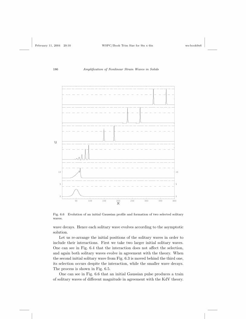
February 11, 2004 20:10 WSPC/Book Trim Size for 9in x 6in ws-book9x6
186 Amplification of Nonlinear Strain Waves in Solids
50 100 150 200 250 300 350 400
x
0
5
10
u
0
5
10
Fig. 6.6 Evolution of an initial Gaussian profile and formation of two selected solitarywaves.
wave decays. Hence each solitary wave evolves according to the asymptoticsolution.
Let us re-arrange the initial positions of the solitary waves in order toinclude their interactions. First we take two larger initial solitary waves.One can see in Fig. 6.4 that the interaction does not affect the selection,and again both solitary waves evolve in agreement with the theory. Whenthe second initial solitary wave from Fig. 6.3 is moved behind the third one,its selection occurs despite the interaction, while the smaller wave decays.The process is shown in Fig. 6.5.
One can see in Fig. 6.6 that an initial Gaussian pulse produces a trainof solitary waves of different magnitude in agreement with the KdV theory.

February 11, 2004 20:10 WSPC/Book Trim Size for 9in x 6in ws-book9x6
Bulk active or dissipative sources of the amplification and selection 187
1 3 5 7 9
x
0
1
2
3
4
5
6
7
u
1 3 5 7 9c
1 3 5 7 9
x
0
1
2
3
4
5
6
7
u
1 3 5 7 9d
1 3 5 7 9
x
0
1
2
3
4
5
6
7
u
1 3 5 7 9a
1 3 5 7 9
x
0
1
2
3
4
5
6
7
u
1 3 5 7 9b
Fig. 6.7 Comparison of asymptotic (dashed line) and numerical (solid line) solutions atvarious ε: a)ε = 0.1, b)ε = 0.3, c)ε = 0.5, d)ε = 1.
Then, the selection of those solitary waves occurs whose amplitudes cometo the selection interval prescribed by the theory. Note that two leadingsolitary waves are selected from below while other solitary waves generatedfrom the input, vanish.
Finally, the influence of the small parameter value is studied. In Fig. 6.7we see that the solitary waves continue to evolve according to the asymp-totic solution with growth in ε. Two main deviations are observed. First isthe difference in amplitudes, it is caused by the increase of the contributionof u1 into the asymptotic solution. The difference in the shape of plateau isshown in Fig. 6.8 where we see the decrease of its length. At larger ε = 10the plateau almost disappears, see Fig. 6.9, however, the initial solitarywave amplitude Q0 = 5 still tends to the value Q2 = 6.38. Selection fromabove still occurs for Q0 > Q2. At the same time we observe a decay of

February 11, 2004 20:10 WSPC/Book Trim Size for 9in x 6in ws-book9x6
188 Amplification of Nonlinear Strain Waves in Solids
1 3 5 7 9 11 13
x
-0.5
-0.4
-0.3
-0.2
-0.1
0
0.1
0.2
u
1 3 5 7 9 11 13c
1 3 5 7 9 11 13 15
x
-0.5
-0.4
-0.3
-0.2
-0.1
0
0.1
0.2
u
1 3 5 7 9 11 13 15d
1 3 5 7 9 11 13 15
x
-0.5
-0.4
-0.3
-0.2
-0.1
0
0.1
0.2
u
1 3 5 7 9 11 13 15a
1 3 5 7 9 11 13 15
x
-0.5
-0.4
-0.3
-0.2
-0.1
0
0.1
0.2
u
1 3 5 7 9 11 13 15b
Fig. 6.8 Comparison of plateau in asymptotic (dashed line) and numerical (solid line)solutions at various ε: a)ε = 0.1, b)ε = 0.3, c)ε = 0.5, d)ε = 1.
the initial solitary wave with the amplitude less than Q0 = 3 that alreadydiffers from the theoretical predictions, Q0 < Q1 = 4.11.
6.3 Moving defects induced by external energy flux
6.3.1 Basic concepts and derivation of governing equations
Recently it was found that point defects may be generated in a solid sub-jected to the laser radiation, see Mirzoev et. al (1996) and references therein.Point defect is described as a distortion in a crystal lattice in the area equalto the atomic volume. The simplest point defects in the crystal are theinterstitial atom, or an atom occupying a position among the atomic equi-librium positions in an ideal lattice, and the vacancy, or a specific site in the

February 11, 2004 20:10 WSPC/Book Trim Size for 9in x 6in ws-book9x6
Bulk active or dissipative sources of the amplification and selection 189
16 18 20 22 24
x
0
1
2
3
4
5
6
u
Fig. 6.9 Evolution of an initial KdV soliton (dashed line) at ε = 10.
lattice of the crystal where atoms are absent Kosevich (1981). Generationof defects due to the laser radiation may be explained using interaction ofstrain, temperature and defect-concentration fields Mirzoev et. al (1996).
Let us consider an isotropic solid where a concentrated energy influx(e.g., laser beam) produces moving point defects. Following Mirzoev et. al(1996) assume nj(x, t) be the concentration of defects of the kind j (j = v
for vacancies, j = i for interstitial atoms) at a point r(x, y, z) at time t.The main processes responsible for the temporal evolution of a defect aregeneration, recombination and diffusion. Then the kinetics of the pointdefects is governed by the equation
nj,t = q0 + qεUx + Djnj,xx − βjnj , (6.51)
where q0 is a velocity of the defects generation in absence of the strain, next

February 11, 2004 20:10 WSPC/Book Trim Size for 9in x 6in ws-book9x6
190 Amplification of Nonlinear Strain Waves in Solids
term in the r.h.s. of Eq.(6.51) accounts for a contribution of a strain intothe defects generation, Dj is the diffusion coefficient of the defect of thekind j, βj is a recombination velocity at sinks Mirzoev and Shelepin (2001).Volume mutual recombination of the defects of different kind is neglected.
It is important that point defects cause deformation of a medium atmacroscopic distances. In elasticity single defect is described by the volumedensity of the force, f ,
f(r) = −K Ω0 ∇δ(r),
where K is the bulk modulus, Ω0 is a dilatation parameter representingthe change in the volume of a crystal as a result of a formation of the onedefect, while defect is located in the coordinate origin Kosevich (1981). Forvacancies we have Ω0 < 0, while Ω0 > 0 corresponds to the interstitialatoms. Combinations of the point defects yield defect of the dipole kindthat may be accounted for
f(r) = −K Ωik ∇kδ(r),
where Ωik is a symmetric tensor. When dipole is axi-symmetric, we have
Ωik = Ω0δik + Ω1(lilk − 1/3δik),
where l is a unit vector of the dipole axis, Ω1 defines deviator of the tensorΩik Kosevich (1981). The average parameters of the crystal specimen maybe introduced if a typical distance between defects is considerably less thanthe gradient of a strain field. Then we have in one-dimensional case
f = −K Ωj nj,x, (6.52)
where evolution of the concentration of defects is accounted for Eq. (6.51).
6.3.2 Nonlinear waves in a medium
One-dimensional governing equation in an elastic medium with moving de-fects may be obtained similar to Eq.(6.12) for a microstructured medium.We start with the coupled equations for nj , Eq.(6.51), and for nonlinearlongitudinal displacement U(x, t),
ρUtt = σx, (6.53)
February 11, 2004 20:10 WSPC/Book Trim Size for 9in x 6in ws-book9x6
Bulk active or dissipative sources of the amplification and selection 191
where σ,
σ = (λ + 2µ)Ux + (3/2(λ + 2µ) + l + 2m)U2x −K Ωj nj .
is written with Eq. (6.52) being taken into account. Equations (6.53),(6.51) are simply uncoupled yielding the governing equation for the strainwaves v = Ux,
vtt − a1vxx − a2( v2)xx − a3vxxt + a4vttt − a5vxxtt + a6vxxxx−
a7( v2)xxt + a8( v2)xxxx = 0, (6.54)
where
a1 =λ + 2µ
ρ− K Ωjqε
ρβj, a2 =
3(λ + 2µ) + 2(l + m) + 3n
4ρ, a3 =
(λ + 2µ)βjρ
,
a4 =1βj
, a5 =Dj
βj, a6 =
(λ + 2µ)Dj
ρβj, a7 =
a2
βj, a8 =
a2Dj
βj.
We see from Eq. (6.54) that presence of the moving defects providesa dispersion in an elastic medium, a5vxxtt and a6vxxxx, as well as dissipa-tive/active terms. The coefficients in Eq.(6.54) do not depend upon K Ωj
with the exception of a1. Equation (6.54) is similar to Eq.(5.42) in Sec. 5.3describing the influence of an external dissipative/active medium on thewaves evolution in a rod. Various simplified cases may be considered:
(i) βj >> 1;(ii) Dj << 1;(iii) βj >> 1, Dj << 1, Dj = O(1/βj).In case (i) recombinations at sinks are strong, quadratic nonlinearity in
Eq.(6.54) predominates, and the formation of shocks is possible. Weaklydispersive case (ii) corresponds to the weak defects diffusion. An analy-sis is already done in Sec. 5.3 where stable kink waves with a ”hat” arefound, see Figs. 5.5, 5.6. Simultaneous weak diffusion and strong recombi-nations in case (iii) provide weakly dissipative/active case which has beenalso studied in Sec. 5.3. When dissipation is negligibly small, the influ-ence of the higher-order nonlinear term a8( v2)xxxx may affect the wavebehavior. Nondissipative limit of Eq.(6.54) is similar to a particular caseof Eq.(1.3) that possesses oscillatory and multi-humps solitary wave solu-tions. However, it was shown in Sec. 1.2 that no stable bell-shaped solitarywaves arise in absence of higher-order derivative terms (like a9 v6x or cor-responding mixed derivative terms) in Eq.(6.54).
February 11, 2004 20:10 WSPC/Book Trim Size for 9in x 6in ws-book9x6
192 Amplification of Nonlinear Strain Waves in Solids
6.3.3 Nonlinear waves in a plate
Equation for longitudinal displacements in a plate already includes a dis-persion even in absence of defects Mirzoev and Shelepin (2001):
Utt − c2sUxx − βNUxUxx − l2(Uttxx − c2
τUxxxx) = −K Ωj
ρnj,x (6.55)
where
c2s =
E
ρ(1− ν2), βN =
3E
ρ(1− ν2)+
2(1− 2ν)ρ(1− ν)3
[(1− 2ν)2l + 2(1− ν + ν2)m],
l2 =ν2h2
12(1− ν)2, c2
τ =µ
ρ(1− ν2),
where h is the width of the plate. Again the evolution of the defects isaccounted for Eq.(6.51). Note that nonlinearity parameter βN does notdepend upon the Murnaghan modulus n.
Uncoupling of Eqs. (6.51), (6.55) in case of the elastic plate is per-formed similar to the previous case giving the governing equation for thelongitudinal strains of the form
vtt − a1vxx − a2( v2)xx − a3vxxtt + a4vxxxx−
b1vxxt + b2vttt − b3( v2)xxt − b4vxxttt + b5vxxxxt+
c1( v2)xxxx + c2vxxxxtt − c3vxxxxxx = 0, (6.56)
where
a1 = c2s −
K Ωjqε
ρβj, a2 =
βN
2, a3 =
Dj
βj+ l2, a4 =
c2sDj
βj+ c2
τ l2,
b1 =c2s
βj, b2 =
1βj
, b3 =βN
2βj, b4 =
l2
βj, b5 =
c2τ l2
βj,
c1 =βNDj
2βj, c2 =
l2Dj
βj, c3 =
c2τ l2Dj
βj.
Equation (6.56) is close to Eq. (5.8) when the ci’s terms in Eq.(6.56)are negligibly small. Now dispersion appears as a result of the plate finitewidth also, and no weakly dispersive case is considered. Case βj >> 1now corresponds to the perturbed double-dispersive equation. There are

February 11, 2004 20:10 WSPC/Book Trim Size for 9in x 6in ws-book9x6
Bulk active or dissipative sources of the amplification and selection 193
two kinds of perturbations. Active/dissipative perturbations are accountedfor the bi’s terms while ci’s terms in Eq.(6.56) play the role of higher-order nonlinearity and dispersion. Hence weakly active/dissipative case isrealized if additionally Dj << 1. Then we can use the results obtainedin Sec. 5.2 to account for the bell-shaped solitary wave selection. WhenDj >> 1, ci’s terms dominate over bi’s terms, and we obtain from Eq.(6.56) the hyperbolic analog of Eq.(1.3) studied in Chapter 1. Thanks tononzero dispersion, now stable oscillatory and multi-humps strain solitarywave solutions are realized, see Figs. 1.7–1.16.
Eqs. (6.51), (6.55) are uncoupled in a different manner if βj << 1. Inthis case Mirzoev and Shelepin (2001) derived the governing equation forthe strain v = Ux,
vt + csvx + βdvxxx + γN v2x = gv − ζvxx + µvxxxx, (6.57)
where
βd =l2(c2
s − c2τ )
2, γN =
βN
ρcs, g =
qεK Ωj
ρc2s
, ζ = βj l2, µ = Dj l
2.
Equation (6.57) may be considered as a perturbed KdV equation. Thenits asymptotic solution is obtained using the procedure explained in Chap-ter 2. The most interesting case is realized when small parameters qε, Dj
and βj are of the same order. Then one can write g = εg∗, ζ = εζ∗, µ = εµ∗,ε << 1. The fast variable θ and the slow time T are introduced as before,θx = 1, θt = −V (T ), T = εt, and the solution of Eq.(6.57) may be obtainedusing the procedure from Chapter 2 to describe the selection of localizedlongitudinal strain wave as a result of the interactions with moving defects.
6.4 Thermoelastic waves
In thermoelasticity the deformation and temperature fields affect eachother. As a result governing equations for the strains and the tempera-ture should be coupled. Very often the influence of the temperature onthe strains is negligibly small. However, thermoelasticity is important tostudy attenuation of the waves that is observed in experiments. Of specialinterest are the processes in polymers arising due to the laser irradiationKartashov and Bartenev (1988). Linear thermoelastic waves were studiedextensively, analytical results for a medium may be found in Kartashov andBartenev (1988); Nowacki (1975); Nowacki (1986b), while numerical simu-

February 11, 2004 20:10 WSPC/Book Trim Size for 9in x 6in ws-book9x6
194 Amplification of Nonlinear Strain Waves in Solids
lations are performed in Berezovski et. al (2000); Berezovski and Maugin(2001). Nonlinear surface wave attenuation is considered in Mayer (1990);Mayer (1995), nonlinear bulk waves are studied in a medium in Engelbrechtand Maugin (1996) and in a rod in Potapov and Semerikova (1988).
Derivation of the equations may be done by various approaches. First,the balance laws are used. In contrast to liquid, the transfer of heat insolids is caused by the heat conduction only. Usually the equation of theheat conduction is obtained from the energy conservation law Engelbrecht(1983); Engelbrecht and Nigul (1981); Landau et. al (1987); Maugin (1995);Maugin (1999); Nowacki (1975); Nowacki (1986b):
T∂S
∂t= div(κ∇T ), (6.58)
where S is the entropy per unit volume, T is the absolute temperature,κ is the thermal conductivity. Usually the last coefficients is assumed tobe constant while the entropy is expressed through the temperature andthe displacements ui. Then Eq. (6.58) is rewritten in the form, see, e.g.,Landau et. al (1987),
Cv∂T
∂t+
Cp − Cv
αT
∂
∂tdiv(u) = κ∇T, (6.59)
where Cp, Cv are the specific heat per unit volume at fixed density andvolume respectively, αT is the heat extension coefficient. The Fourier lawof thermal conduction, Q = −κ∇T , is used to obtain Eqs. (6.58), (6.59).However, it predicts an infinite velocity of a thermal wave. In order todescribe the finite velocity, the modification of the law is needed. In par-ticular, the generalized law has been proposed in Likov (1967)
Q = −κ∇T − τ∗Qt,
that takes into account an inertia of the heat flux, τ∗ is a time of the heatflux relaxation.
Balance of linear momentum provides the second equation of thermoe-lasticity,
ρ0utt = DivP∗, (6.60)
where P∗ is the Piola-Kirchoff tensor expressed through the free energydensity W (u,T ), P∗ = ∂W/∂∇u. Usually only the term linear in ∇u,αT (T − T0)∇u, is included into W . Hence Eq.(6.60) contains the linear

February 11, 2004 20:10 WSPC/Book Trim Size for 9in x 6in ws-book9x6
Bulk active or dissipative sources of the amplification and selection 195
term depending on the temperature while nonlinearity is caused by thesame reasons as in pure elastic case, see Chapter 3.
Equations of thermoelasticity may be derived using the variationalmethods Fares (2000); Maugin (2000); Nowacki (1975); Nowacki (1986b);Rayleigh (1945). However, usually only Eq.(6.60) is derived from theHamilton principle while the heat equation is introduced additionally Fares(2000). It was Maugin (2000) who proposed the modification of the freeenergy density so as to get all field equations, balance laws and constitutiverelations for the theory of materially inhomogeneous, finitely deformable,thermoelastic conductors of heat, in the same manner. The main idea is toassume a dependence upon an additional variable called thermacy whosetemporal derivative is the temperature. As a result all equations obtainedturn out strict conservation laws. Classical dissipative thermoelastic equa-tions are obtained by isolation the contribution of the thermacy.
6.4.1 Nonlinear waves in thermoelastic medium
Below we follow Engelbrecht and Maugin (1996) where one-dimensionalmodel is considered using the notion of thermodynamic internal variables.The evolution nonlinear equation is obtained for the observable variable(longitudinal strain v = Ux(x, t)) in a medium when temperature T (x, t)effects are considered as internal process. The equation of motion,
ρ0Utt−(λ+2µ)Uxx−[3(λ+2µ)+2l+4m]UxUxx = −(3λ+2µ)αT Tx, (6.61)
is coupled with the energy equation for the temperature,
ρ0CvTt + T0(3λ + 2µ)αT Uxt = κTxx. (6.62)
Single nonlinear model equation may be obtained in case of a weak coupling,ε = (3λ + 2µ)αT /ρ0, ε << 1. Introducing fast and slow variables, ξ =c0t−X, τ = εX, one obtains for w = Ut
wt + a1 wwξ + Λ w = 0, (6.63)
where
a1 =3(λ + 2µ) + 2l + 4m
(λ + 2µ)εc0, Λ =
T0((3λ + 2µ)αT )2
2ερ0c0κ, c2
0 =λ + 2µ
ρ0.
Exact solution of Eq.(6.63) is known Whitham (1974), it may include shockswhen the gradient of the initial excitation is large enough.

February 11, 2004 20:10 WSPC/Book Trim Size for 9in x 6in ws-book9x6
196 Amplification of Nonlinear Strain Waves in Solids
When the coupling is not weak, Eqs. (6.61), (6.62) are transformed byanother way, the case was not considered in Engelbrecht and Maugin (1996).First, the temperature gradient, Tx, is expressed through the displacementusing Eq.(6.61). Then it is substituted into Eq.(6.62) differentiated withrespect to x, yielding nonlinear equation for U
(ρ0Cvc20+Λ1)Uxxt−ρ0CvUttt+a2(U2
x)xt+κ(Uxxtt−c20Uxxxx−a2(U2
x)xxx) = 0,
(6.64)where
a2 =3(λ + 2µ) + 2l + 4m
2ρ0, Λ1 =
T0((3λ + 2µ)αT )2
ρ0.
In the reference frame, ξ = x− V t, the ODE reduction of Eq.(6.64) iswritten for the function v = Uξ
∂2
∂ξ2
(b1v + b2v
2 + b3vξ + b4(v2)ξ
)= 0,
with
b1 = V (ρ0CvV 2 − ρ0Cvc20 − Λ1), b2 = −a2V,
b3 = κ(V 2 − c20), b4 = −a2κ.
There is a similarity with the Burgers equation model if the last non-linear term is negligibly small. The Burgers model has been developed inEngelbrecht (1983), with the relaxation tame taken into account. Compar-ison of the Burgers equation model and the model governed by Eq.(6.63)is done in Engelbrecht and Maugin (1996).
6.4.2 Longitudinal waves in thermoelastic rod
As already noted, thermal conduction weakly affects strain waves in solids.More promising looks the influence of a heat transfer through the lateralsurface of a wave guide, especially caused by a laser irradiation, see Kar-tashov and Bartenev (1988); Mirzoev et. al (1996) and references therein.The influence of the external heat transfer on nonlinear longitudinal strainwaves in a rod has been studied in Potapov and Semerikova (1988). Esti-mations done there demonstrate the dominant role of the heat transfer incomparison with the thermal conduction mechanism.
The coupled equations of thermoelasticity are used in Potapov and Se-merikova (1988) with the heat transfer boundary conditions on the rod

February 11, 2004 20:10 WSPC/Book Trim Size for 9in x 6in ws-book9x6
Bulk active or dissipative sources of the amplification and selection 197
lateral surface being taken into account:
Utt − c2sUxx − β UxUxx + 0.5R2(ν(1− ν)Uttxx − νc2
sUxxxx) = −αT c2s Tx,
(6.65)
ρ0CvR Tt − κR Txx + 2h(T − T0) = −αT ET0R Uxt, (6.66)
where β is a nonlinear coefficient, β = ρ−10 (3E + l(1−2ν)3 +4m(1−2ν)(1+
ν) + 6nν2), R is a radius of the rod, T0 is a constant temperature of anexternal medium, h is a heat transfer coefficient, c2
s = E/ρ0 is a velocity ofthe linear waves in a rod. Note that the dispersion terms coefficient fromPotapov and Semerikova (1988) are corrected here in accordance with theprocedure from Chapter 3.
Let us differentiate Eq.(6.66) with respect to x and substitute Tx fromEq.(6.65). Then the governing equation for longitudinal displacementsholds,
∂
∂tρ0Utt −E
(1 +
α2T ET0
ρ0Cv
)Uxx − β UxUxx +
ρ0ν(1− ν)R2
2Uttxx−
νER2
2Uxxxx =
(κ
ρ0Cv
∂2
∂x2− 2h
ρ0CvR
)ρ0Utt − EUxx−
β UxUxx +ρ0ν(1− ν)R2
2Uttxx − νER2
2Uxxxx. (6.67)
We are dealing with elastic strain waves whose magnitude B is small,B << 1, and with long waves with typical length L, so as R/L << 1. Asusual we consider the case of a balance between nonlinearity and dispersionintroducing small parameter ε = B = (R/L)2. Contribution of the termsin the r.h.s. of Eq.(6.67) is weak, they may be considered as small pertur-bations. Then nonlinear and dispersive terms may be omitted in the r.h.s.Obviously,
Uxx =ρ20Cv
E(ρ0Cv + α2T ET0)
Utt + O(ε).
Hence the simplest equation accounting for the influence of both theheat transfer and thermal conduction on longitudinal strain waves v = Ux
is

February 11, 2004 20:10 WSPC/Book Trim Size for 9in x 6in ws-book9x6
198 Amplification of Nonlinear Strain Waves in Solids
vtt − c2s(1 +
α2T c2
sT0
Cv)vxx − β
2ρ0(v2)xx +
ν(1− ν)R2
2vttxx − νc2
sR2
2vxxxx =
α2T c2
sT0
Cv + α2T c2
sT0
(κ
ρ0Cvvttx − 2h
ρ0CvRvt
). (6.68)
Certainly Eq.(6.68) may be studied by the methods developed in Chap-ter 2 to account for an amplification, attenuation and selection of longitu-dinal thermoelastic waves.

February 11, 2004 20:10 WSPC/Book Trim Size for 9in x 6in ws-book9x6
Bibliography
Ablowitz, M. J. and Segur, H.(1981) Solitons and the Inverse Scattering Trans-form, SIAM, Philadelphia.
Akhmediev, N.N. and Ankiewicz, A. (1997) Solitons. Nonlinear pulses and beams,Chapman & Hall, London.
Alekseev, V.N. and Rybak S.A. (2002) ”Equations of state for viscoelastic bio-logical media”, Acoust. J. 48, 511.
Alexeyev, A.A.(1999) ”Classical and non-classical interactions of kinks in somebubbly medium”, J. Phys. A 32, 4419.
Bateman, G. and Erdelyi, A. (1953-54). Higher Transcendental Functions, vol. 3,McGraw Hill, New York.
Belokolos, A., Bobenko, A., Enol’skij, V., Its, V. and Matveeev, V. (1994)Algebro- Geometrical Approach to Nonlinear Integrable Equations, Springer,Berlin.
Benilov, E.S., Grimshaw, R., Kuznetsova, E.P.(1993) ” The generation of radiat-ing waves in a singularly-perturbed KdV equation”, Physica D 69 270.
Berezin, Ya. A. (1987) Modelling Non-Linear Wave Processes. VNU SciencePress, Utrecht.
Berezovski, A., Engelbrecht, J., Maugin, G.A. (2000) ”Thermoelastic wave prop-agation in inhomogeneous media”, Arch. Appl. Mech. 70, 694.
Berezovski, A. and Maugin, G.A. (2001) ”Simulation of Thermoelastic WavePropagation by Means of a Composite Wave-Propagation Algorithm”, J.Compt. Phys. 168, 249.
Bhatnagar, P.L. (1979) Nonlinear Waves in One-Dimensional Dispersive Sys-tems, Claredon Press, Oxford.
Biryukov, S.V., Gulyaev, V.V., Krylov, V.V. and Plessky, V.P. (1991) Surfaceacoustic waves in inhomogeneous media, Nauka, Moscow (in Russian).
Bland, D. R. (1960) The Theory of Linear Viscoelasticity, Oxford .Bland, D.R.(1969) Nonlinear Dynamic Elasticity, Blaisdell, Waltham, Mass et al.Boyd, J. P. (1991) ”Weakly non-local solitons for capillary-gravity waves: the
fifth-degree Korteweg-de Vries equation”, Physica D 48, 129.Bridges, T. (1986) ”Cnoidal standing waves and the transition to the travelling
hydravlic jump”, Phys. Fluids 29, 2819.
199

February 11, 2004 20:10 WSPC/Book Trim Size for 9in x 6in ws-book9x6
200 Book Title
Bukhanovsky, A.V. and Samsonov, A.M. (1998) ”Numerical Simulation of Nonlin-ear Elastic waves in Inhomogeneous Wave Guides”, St. Petersburg, Preprintof the Institute for High performance Computing and Data Bases No 6-98(in Russian).
Bullough, R.K. and Caudrey, P.J. eds., (1980) Solitons, Springer, Berlin.Burgers, J.M. (1948) ”A Mathematical model illustrating the theory of turbu-
lence”, Adv. Appl. Mech. 1, 171.Byrd, P.F. and Friedman, M.D. (1954) Handbook of Elliptic Integrals for Engi-
neers and Physicists, Springer, Berlin.Calogero, F. and Degasperis, A. (1982) Spectral Transform and Solitons, North-
Holland, Amsterdam.Cariello, F. and Tabor, M.(1989) ”Painleve expansions for nonintegrable evolution
equations”, Physica D 39, 77.Capriz, G. (1989) Continua with microstrucure, Springer Tracts in Nat. Phil.,
V.35, Springer, Berlin.Cermelli, P. and Pastrone, F. (1997) ”Growth and decay of waves in microstruc-
tured solids”, Proc. Estonian Acad. Sci. Phys. Math. 46, 32.Chang, H.-C., Demekhin, E.A., and Kopelevich, D.I. (1995) ”Stability of a Soli-
tary Pulse against Wave Packet Disturbances in an Active Media”, Phys.Rev. Lett. 75, 1747.
Chow, K.W. (1995) ”A class of exact, periodic solutions of nonlinear envelopeequations”, J. Math. Phys. 36, 4125.
Christensen, R.M. (1971) Theory of Viscoelasticity, Academic Press, New York.Christiansen, P.L., Eilbeck, J.C., Enolskii, V.Z., Kostov, N.A. (1995) ”Quasi-
periodic solutions of the coupled nonlinear Schrodinger equations”, Proc.R. Soc. Lond. A 451, 685.
Christou, M.A. and Christov, C.I. (2000) ”Fourier-Galerkin Method for Local-ized Solutions of the sixth-order Generalized Boussinesq Equation”, Proc.Intern. Conf. on Dynamical Systema and Differential Equations, May 18-21, Atlanta, USA, 121.
Christou, M.A. and Christov, C.I. (2002) ”Fourier-Galerkin Method for LocalizedSolutions of the Equations with Cubic Nonlinearity”, J. Comp. Anal. Appl.4, 63.
Christov, C.I. (1994) ”Numerical Investigation of the long-time evolution andinteraction of localized waves”, in Fluid Physics, eds. Velarde, M.G. &Christov, C.I., World Scientific, Singapore, 353.
Christov, C.I. and Maugin, G.A. (1995) ”An Implicit Difference Scheme for theLong-Time Evolution of Localized Solutions of a Generalized BoussinesqSystem”, J. Compt. Phys. 116, 39.
Christov, C.I., Maugin, G.A., Velarde, M.G. (1996) ”Well-posed Boussinesqparadigm with purely spatial higher-order derivatives”, Phys.Rev. E 54,3621.
Christov, C.I., Pontes, J., Walgraef, D., and Velarde, M.G. (1997) ”Implicittime splitting for fourth-order parabolic equations”, Comput. Methods Appl.Mech. Engrg. 148, 209.

February 11, 2004 20:10 WSPC/Book Trim Size for 9in x 6in ws-book9x6
Chapter Title for Bibliography 201
Christov, C.I. and Velarde, M.G. (1994) ”Inelastic Interactions of BoussinesqSolitons”, Intern. J. Bif. Chaos 4, 1095.
Christov, C.I. and Velarde, M.G. (1995) ”Dissipative solitons”, Physica D 86,323.
Cole, J.D. (1968) Perturbation Methods in Applied Mathematics, Blaisdell,Waltham, Mass.
Conte, R. (1989) ”Invariant Painleve analysis of partial differential equations”,Phys. Lett. A 140, 383.
Conte, R., Fordy, A., Pickering, A. (1993) ”A perturbative Painleve approach tononlinear differential equations”, Physica D 69, 33.
Crighton, D.G. (1995) ”Applications of KdV”, Acta Applicandae Mathematicae39, 39.
Dai, H.-H. (1998) ”Model equations for nonlinear dispersive waves in a compress-ible Mooney-Rivlin rod”, Acta Mech. 127, 193.
Dodd, R.K., Eilbeck, J.C., Gibbon, J.D. and Morris, H.C. (1982) Solitons andNonlinear Wave Equations, Academic Press, London et al.
Drazin, P.G. and Johnson, R.S. (1989) Solitons: an Introduction, CambridgeUniv. Press, Cambridge.
Dreiden, G.V., Porubov, A.V., Samsonov, A.M., Semenova, I.V., and Sokurin-skaya, E.V. (1995) ”Experiments in the propagation of longitudinal strainsolitons in a nonlinearly elastic rod”, Tech. Phys. Lett 21, 415.
Dreiden, G.V. , Porubov, A.V., Samsonov, A.M., Semenova, I.V. (2001) ”Reflec-tion of a longitudinal strain solitary wave from the end face of a nonlinearlyelastic rod”, Tech.Phys. 46, no 5, 505.
Elmer, F.-J. (1997) ”Nonlinear dynamics of dry friction”, J. Phys. A: Math. Gen.,30, 6057.
Engelbrecht, J. (1979) ”One-Dimensional Deformation waves in Nonlinear Vis-coelastic Media”, Wave Motion 1, 65.
Engelbrecht, J. (1983) Nonlinear wave processes of deformation in solids, Pitman,Boston.
Engelbrecht, J. ed. (1989) Nonlinear Waves in Active media, Springer-Verlag,Berlin.
Engelbrecht, J. (1997) Nonlinear Wave Dynamics. Complexity and Simplicity,Kluwer, The Netherlands.
Engelbrecht, J. and Braun, M. (1998) ”Nonlinear waves in nonlocal media”, Appl.Mech. Rev. 51, No 8, 475.
Engelbrecht,J., Cermelli, P. and Pastrone, F. (1999) ”Wave hierarchy in mi-crostructured solids”, In: Geometry, Continua and Microstructure. Ed. byG.A. Maugin, Herman Publ., Paris, 99.
Engelbrecht, J. and Khamidullin, Y. (1988) ”On the possible amplification ofnonlinear seismic waves”, Phys. Earth Planet. Inter. 50, 39.
Engelbrecht, J. and Maugin, G.A. (1996) ”Deformation waves in thermoelasticmedia and the concept of internal variables”, Arch. Appl. Mech. 66, 200.
Engelbrecht, J. and Nigul, U. (1981) Nonlinear Deformation Waves, Nauka,Moscow (in Russian).

February 11, 2004 20:10 WSPC/Book Trim Size for 9in x 6in ws-book9x6
202 Book Title
Erbay, S., Erbay, H.A., and Dost, S. (1991) ”Nonlinear wave modulation in mi-cropolar elastic media-I. longitudinal waves” Int. J. Engng. Sci. 29, 845.
Eringen, A. C. (1968). Theory of micropolar elasticity. P. 622. In: Fracture. Anadvanced treatise. V.2. Mathematical fundamentals. Ed. by H. Liebowitz,Academic Press, New York.
Eringen, A.C. and Suhubi, E.S. (1964) ”Nonlinear theory of micro-elastic solids”,Intern. J. Eng. Sci. 2, Part I, 189, Part II, 389.
Erofeev, V.I. (2002) Wave processes in solids with microstructure, World Scien-tific, Singapore.
Erofeev, V.I. and Klyueva, N.V. (2002) ”Solitons and nonlinear periodic strainwaves in rods, plates and shells”, Acoust. J. 48, 725 (in Russian).
Erofeev, V.I. and Potapov, A.I. (1993) ”Longitudinal strain waves in non-linearlyelastic media with couple stresses”, Int. J. Nonl. Mech. 28, 483.
Fares, M.E. (2000) ”Generalized non-linear thermoelasticity for composite lami-nated structures using a mixed variational approach”, Int. J. Nonl. Mech.35, 439.
Feng, B.F. and Kawahara, T. (2000) ”Stationary travelling-wave solutions of anunstable KdV-Burgers equation”, Physica D 137, 228.
Fletcher, C.A.J. (1984) Computational Galerkin Methods, Springer, Berlin.Fowler, A.C. (1997) Mathematical Models in the Applied Sciences, Cambridge
Univ. Press, Cambridge.Frantsevich, I.N., Voronov, F.F., and Bakuta, S.A. (1982) Elastic Constants and
Moduli of Metals and Nonmetals, Naukova Dumka, Kiev, (in Russian).Galin, L.A. (1980) Contact problems of elasticity and viscoelasticity, Nauka,
Moscow (in Russian).Garazo, A.N. and Velarde, M.G. (1991) ”Dissipative Korteweg-de Vries descrip-
tion of Marangoni-Benard oscillatory convection”, Phys. Fluids A 3, 2295.Godunov, S.K. and Ryaben’kii, V.S. (1973) Difference Schemes, Nauka, Moscow,
(in Russian).Godunov, S.K. and Ryaben’kii, V.S. (1987) Difference Schemes: introduction to
the underlying theory of, North-Holland, Amsterdam.Godunov, S.K. (1997) Ordinary Differential Equations with Constant Coefficients,
AMS.Goryacheva, I.G. (1998) Contact mechanics in tribology, Dordrecht etc., Kluwer.Goryacheva, I.G. (2001) Mechanics of friction interaction, Nauka, Moscow (in
Russian).Grimshaw, R., Malomed, B. and Benilov, E. (1994) ” Solitary waves with damped
oscillatory tails: an analysis of the fifth-order Korteweg-de Vries equation”,Physica D 77, 4783.
Grimshaw R, Pelinovsky E. and Talipova T. (1999) ”Solitary wave transformationin a medium with sign-variable quadratic nonlinearity and cubic nonlinear-ity”, Physica D 132, 40.
Gulyaev, Yu.V. and Polsikova, N.I. (1978) ”Shear surface acoustic waves on acylindriucal surface of a solid body covered by a layer of a foreign material”,Sov. Phys- Acoust. R. 24, 287.

February 11, 2004 20:10 WSPC/Book Trim Size for 9in x 6in ws-book9x6
Chapter Title for Bibliography 203
Gusev, A. A. (1988) Two dilatancy-based models to explain coda-wave precursorsand P/S spectral ratio. Tectonophysics 152, 227.
Hahner, G. and Spencer, N. (1998) ”Rubbing and scrubbing”, Physics Today,No 9, 22.
Harker, A.N. (1988) Elastic Waves in Solids with Application to NondestructiveTesting of Pipelines, Hilger & Bristol, Philadelphia.
Hunter, J.K. and Scheurle, J. (1988) ”Existence of perturbed solitary wave solu-tions to a model equation for water waves”, Physica D 32, 253.
Ince, E. (1964) Ordinary Differential Equations, Dover, New York.Jeffrey, A. and Kawahara, T. (1982) Asymptotic Methods in Nonlinear Wave
Theory, Pitman, London.Jeffrey, A. and Engelbrecht, J., eds. (1994) Nonlinear Waves in Solids, Springer,
Wien.Johnson, K.L. (1985) Contact Mechanics, Cambridge Univ. Press, Cambridge.Kalker, J.J., Dekking, F.M., and Vollebregt, E.A.H. (1997) ”Simulation of Rough,
Elastic Contacts”, J. Appl. Mech. 64, 361.Kano, K. and Nakayama, T. (1981) ”An Exact Solution of the Wave Equation
ut + u ux − u5x = 0”, J. Phys. Soc. Jpn. 50, 361.Karpman, V. I. (1993) ”Radiation by solitons due to higher-order dispersion”,
Phys.Rev. E 47, 2073.Karpman, V.I. and Vanden-Broeck, J.-M. (1995) ”Stationary solitons and stabi-
lization of the collapse described by KdV-type equations with high nonlin-earities and dispersion”, Phys. Lett. A 200, 423.
Karpman, V.I. (1998) ”Evolution of radiating solitons described by the fifth orderKorteweg-de Vries type equations”, Phys. Lett. A 244, 394.
Karpman, V.I. (2001) ”Stability of solitons described by KdV-type equations withhigher-order dispersion and nonlinearity (analytical results)”, Phys. Lett. A284, 246.
Kartashov, E.M. and Bartenev, G.M. (1988) ”Dynamic effects in solid underinteractions with intensive heat fluxes”, Itogi Nauki i tekhniki, Ser.: Khimiai tekhnologia visokomolekuliarnikh soedinenii” 25, 3 (in Russian).
Kascheev, V.N. (1990) Heuristic Approach to Obtain Solutions to Nonlinear Equa-tions of Solitonics, Zinatne, Riga (in Russian).
Kawahara, T. (1972) ”Oscillatory Solitary Waves in Dispersive Media”, J. Phys.Soc. Jpn. 33, 260.
Kawahara, T. (1983) ” Formation of saturated solitons in a nonlinear dispersivesystem with instability and dissipation” Phys. Rev. Lett. 51, 381.
Kawahara, T. and Takaoka, M. (1988) ”Chaotic Motions in an Oscillatory SolitonLattice”, J. Phys. Soc. Jpn. 57, 3714.
Kerr, A.D. (1964) ”Elastic and viscoelastic foundation models”, J. Appl. Mech.31, 491.
Kliakhandler, I.L. (1999) http://www.math.mtu.edu/˜igorKliakhandler, I.L. , Porubov, A.V. and Velarde, M.G. (2000) ”Localized finite-
amplitude disturbances and selection of solitary waves”, Phys. Rev. E 62,4959.

February 11, 2004 20:10 WSPC/Book Trim Size for 9in x 6in ws-book9x6
204 Book Title
Kodama, J. and Ablowitz, M. (1981) ”Perturbation of solitons and solitarywaves”, Stud. Appl. Math. 64, 225.
Korpel, A. and Banerjee, P. (1984) ”Heuristic guide to nonlinear dispersive waveequations and soliton-type solutions”, IEEE 72, 1109.
Korteweg, D.J. and de Vries, G. (1895) ”On the change of the form of long wavesadvancing in a rectangular channel and on a new type of long stationarywaves”, Phil. Mag. 5, 422.
Kosevich, A.M. (1981) Physical Mechanics of Real Crystals, Naukova Dumka,Kiev (in Russian).
Kosevich, A.M. and Savotchenko, S.E. (1999) ”Features of dynamics of one-dimensional discrete systems with non-neighbouring interactions, and roleof higher-order dispersion in solitary wave dynamics”, Low Temp. Phys. 25,737 (in Russian).
Kostov, N.A. and Uzunov, I.M. (1992) ”New kinds of periodical waves in bire-fringent optical fibers”, Opt. Comm. 89, 389.
Kozak, J. and Sileny, J. (1985) ”Seismic events with non-shear component. I.Shallow earthquakes with a possible tensile source component”. PAGEOPH123, 1.
Kudryashov, N.A. (1988)” Exact solitonic solutions of the generalized evolutionequation of wave dynamics”, J. Appl. Math. Mech. 52, 361.
Landau L.D., Lifshitz E.M., Kosevich, A.M., and Pitaevsky, L.P. (1987) Theoryof Elaticity, Pergamon Press, Oxford.
Levi, D. and Winternitz, P. , eds. (1992) Painleve Transcendents: Their Asymp-totics and Physical Applications, Plenum Press, New York and London.
Likov, B. Ya. (1967) Theory of thermal conduction, Nauka, Moscow (in Russian).Lou, S., Huang, G. and Ruan, H. (1991) ”Exact solitary waves in a convecting
fluid”, J. Phys. A 24, L587.Love, A.E.H. (1927) A Treatise on the Mathematical Theory of Elasticity, Uni-
versity Press, Cambridge.Lurie, A.I. (1990) Nonlinear Theory of elasticity, Amsterdam, Elsevier.Marchant, T.R. (1996) ”The evolution and interaction of Marangoni-Benard soli-
tary waves”, Wave Motion 23, 307Maugin, G.A. (1990) ”Internal Variables and Dissipative Structures”, J. Non-
Equilib. Thermodyn. 15, 173.Maugin, G.A. (1993) Material Inhomogeneities in Elasticity, Chapman & Hall,
London.Maugin, G.A. (1995) ”Material forces: Concepts and applications”, Appl. Mech.
Rev. 48, 213.Maugin, G.A. (1999) The Thermomechanics of Nonlinear Irreversible Behaviors.
An Introduction., World Scientific, Singapore.Maugin, G.A. (2000) ”Towards an analytical mechanics of dissipative materi-
als” Rendiconti del Seminario Matematico dell’Universita’ e Politecnico diTorino 58, 171.
Maugin, G.A. and Muschik, W. (1994) ”Thermodynamics with internal variables”J.Non-Equil. Thermodyn. 19, 217.

February 11, 2004 20:10 WSPC/Book Trim Size for 9in x 6in ws-book9x6
Chapter Title for Bibliography 205
Mayer, A (1990) ”Thermoelastic attenuation of surface acoustic waves in coatedelastic media”, J. Appl. Phys. 68, 5913.
Mayer, A (1995) ”Surface Acoustic Waves in Nonlinear Elastic Media”, Phys.Reports 256, 257.
Miloserdova, I.V. and Potapov, A.I. (1983) ”Nonlinear standing waves in a rodof finite length”, Sov. Phys. Acoust., 29, 306.
Mindlin, R.D. (1964) ”Microstructure in linear elasticity”, Arch. Rat. Mech. Anal.No1, 51.
Mirzoev, F. Kh., Panchenko, V. Ya, Shelepin, L.A. (1996) ”Laser Control ofProcesses in Solids”, Physics- Uspekhi 39, 1.
Mirzoev, F. Kh., and Shelepin, L.A. (2001) ”Nonlinear Strain Waves and Densitiesof Defects in Metal Plates Induced by External Energy Fluxes”, Tech. Phys.46, 952.
Morton, K.W. and Mayers, D.F. (1994) Numerical Solution of Partial DifferentialEquations, Cambridge University Press, Cambridge.
Murnaghan, F.D. (1951) Finite Deformations of an Elastic Solid, J. Wiley, NewYork.
Nakamura, A. (1979) ”A direct method of calculating periodic wave solutionsto nonlinear evolution equations. I. exact two-periodic wave solution”, J.Phys. Soc. Jpn. 47, 1701.
Nagashima, H. and Kuwahara, M. (1981) ”Computer Simulation of SolitaryWaves of the Nonlinear Wave Equation ut + u ux − γ2 u5x = 0” J. Phys.Soc. Jpn. 50, 3792.
Nayfeh, A.H. (1973) Perturbation Methods, J. Wiley & Sons, New York.Nekorkin, V.I. and Velarde, M.G. (1994) ”Solitary waves, soliton bound states
and chaos in a dissipative Korteweg-de Vries equation”, Int. J. Bif. Chaos4, 1135.
Nepomnyashchy, A.A. and Velarde, M.G. (1994) ”A three-dimensional descriptionof solitary waves and their interaction in Marangoni-Benard layers”, Phys.Fluids A 6, 187.
Newell, A (1985) Solitons in Mathematics and Physics, SIAM, Philadelphia.Newell, A., Tabor, M., Zeng, Y.B. (1987) ”A Unified Approach to Painleve Ex-
pansions”, Physica D 29, 1.Newille, E.H. (1951) Jacobian Elliptic Functions, Claredon Press, Oxford.Nikitin, L.V. (1998) Statics and dynamics of solids with external dry friction,
Moscovskii Licei, Moscow (in Russian).Nikolaev, A.V. (1989) ”Scattering and dissipation of seismic waves in presence of
nonlinearity”, PAGEOPH 131, 687.Nikolova, E.G. (1977) ”On the effective surface tension of solid bodies”, Sov.
Phys. JETP 45, 285.McNiven, H.D. and McCoy, J.J. (1974) ”Vibrations and wave propagation in
rods”, in: G. Herrmann ed., R. Mindlin and Applied Mechanics, Pergamon,New York , p. 197.
Nowacki, W. (1975) Theory of Elasticity, Mir, Moscow (in Russian).Nowacki, W. (1986a) Theory of Asymmetric Elasticity, Pergamon, Oxford.Nowacki, W. (1986b) Thermoelasticity, Pergamon, Oxford.

February 11, 2004 20:10 WSPC/Book Trim Size for 9in x 6in ws-book9x6
206 Book Title
Oliner, A.A. ed. (1978) Surface Acoustic Waves. Springer-Verlag, Berlin.
Oron, A. and Rosenau, P. (1997) ”Evolution and formation of dispersive-dissipative patterns”, Phys. Rev. E 55, R1267.
Ostrovsky, L.A. and Potapov, A.I. (1999) Modulated waves in linear and nonlinearmedia, The John Hopkins University Press, Baltimore.
Parker, D.F. (1994) ”Nonlinear Surface Acoustic Waves and Waves on StratifiedMedia”, In: A.Jeffrey and J. Engelbrecht, eds. , Nonlinear Waves in Solids,Springer, Berlin.
Parker, D.F. and Maugin, G.A. , eds. (1987) Recent Developments in SurfaceAcoustic waves, Springer, Berlin.
Parker, D.F. and Mayer, A. (1991) ” Dissipation of Surface Acoustic Waves”,In: D.Fusco and A. Jeffrey, eds., Nonlinear Waves and Dissipative Effects,Longman, London.
Parker, D.F. and Tsoy, E.N. (1999) ”Explicit Solitary and Periodic Solutions forOptical Cascading”, J. Eng. Math. 36, 149.
Parkes, E.J. and Duffy, B.R. (1996) ”An automated tanh-function method forfinding solitary wave solutions to nonlinear evolution equations”, ComputerPhys. Comm. 98, 288.
Pasternak, P.L. (1954) On a New Method of Analysis of an elastic Foundationbe Means of Two Foundation Constants (in Russian), Gosudarstvennoe Iz-datel’stvo Litearturi po Stroitel’stvu i Arkhitekture, Moscow, USSR (inRussian).
Porubov, A.V. (1993) ”Exact travelling wave solutions of nonlinear evolutionequation of surface waves in a convecting fluid”, J. Phys. A: Math. Gen.26, L797.
Porubov, A.V.(1995) Free Surface Nonlinear Waves on a viscous inhomogeneousliquid layer. Ph.D. Thesis, State Technical University, Saint Petersburg ( inRussian).
Porubov, A.V. (1996) ”Periodical solution to the nonlinear dissipative equationfor surface waves in a convective liquid layer”, Phys. Lett. A 221, 391.
Porubov, A.V. (2000) ”Strain solitary waves in an elastic rod with microstruc-ture”, Rendiconti del Seminario Matematico dell’Universita’ e Politecnicodi Torino 58, 189.
Porubov, A.V., Gursky, V.V. and Maugin, G.A. (2003) ”Selection of localizednonlinear seismic waves”, Proc. Estonian Acad. Sci., Phys. Math. 52, No1.
Porubov, A.V., Maugin, G.A., Krzhizhanovskaya, V.V. and Gursky, V.V. (2002)”Influence of higher- order dispersion and nonlinearity on solitary waveformation from an initial localized pulse”, submitted for publication
Porubov, A.V. and Parker, D.F. (1999) ”Some General Periodic Solutions toCoupled Nonlinear Schrodinger Equations”, Wave Motion 29, 97.
Porubov, A.V. and Parker, D.F. (2002) ”Some General Periodic Solutions forOptical Cascading”, Proc. Roy. Soc. A 458, 2139.

February 11, 2004 20:10 WSPC/Book Trim Size for 9in x 6in ws-book9x6
Chapter Title for Bibliography 207
Porubov, A.V. and Pastrone, F. (2001) ”Influence of macro- and microdissipationon nonlinear strain solitary wave evolution”. Quaderni del Dipartimento diMatematica N. 56, University of Turin, Turin.
Porubov, A.V. and Samsonov, A.M. (1993) ”Refinement of the model for thepropagation of longitudinal strain waves in a rod with nonlinear elasticity”,Tech. Phys. Lett. 19, 365.
Porubov, A.V. , Samsonov, A.M. , Velarde, M.G. and Bukhanovsky, A.V. (1998)”Strain solitary waves in an elastic rod embedded in another elastic externalmedium with sliding”, Phys.Rev. E 58, 3854 .
Porubov, A.V. and Velarde, M.G. (1999) ”Exact Periodic Solutions of the Com-plex Ginzburg-Landau Equation”, J. Math. Phys. 40, 884.
Porubov, A.V. and Velarde, M.G. (2000) ”Dispersive-dissipative solitons in non-linear solids”, Wave Motion 31, 197.
Porubov, A.V. and Velarde, M.G. (2002) ”Strain kinks in an elastic rod embeddedin a viscoelastic medium”, Wave Motion 35, 189.
Poschel, T. and Herrmann, H.J. (1993) ”A simple geometrical model for solidfriction”, Physica A 198, 441.
Potapov, A.I. and Rodyushkin, V.M. (2001) ”Experimental study of strain wavesin materials with microstructure”, Acoust. J. 47, 347.
Potapov, A.I. and Semerikova, N.P. (1988) ”Nonlinear longitudinal waves in a rodtaking into account the interaction between strain and temperature fields”,Sov. Appl. Mech. and Tech. Phys., No1, 54.
Qaisar, M. (1989) ”Attenuation Properties of Viscoelastic Material” PAGEOPH131, 703.
Rayleigh Lord (J.W. Strutt) (1945) Theory of Sound, Vol. 1, Reprint, Dover, NewYork.
Rednikov, A. Ye., Velarde, M.G., Ryazantsev, Yu. S., Nepomnyashchy, A.A.,and Kurdyumov V.N., (1995) ”Cnoidal Wave Trains and Solitary Wavesin a Dissipation Modified Korteweg- de Vries Equation”, Acta ApplicandaeMathematicae 39, 457.
Richtmyer, R.D. and Morton, K.W. (1967) Difference Methods for Initial-ValueProblems, Wiley & Sons, New York.
Sachdev, P.L. (1987) Nonlinear diffusive waves, Cambridge Univ. Press, Cam-bridge.
Salupere, A., Maugin, G.A., Engelbrecht, J. (1994) ”Korteweg-de Vries solitondetection from a harmonic input”, Phys. Lett. A 192, 5.
Salupere, A. , Maugin, G.A. and Engelbrecht, J. (1997) ”Solitons in systems witha quartic potential and higher-order dispersion”, Proc. Estonian Acad. Sci.,Phys. Math. 46, 118.
Salupere, A. , Engelbrecht, J. and Maugin, G.A. (2001) ”Solitonic structures inKdV-based higher-order systems”, Wave Motion 34, 51.
Samarskii, A.A. and Nikolaev, E.S. (1989) Numerical Methods for Grid Equations,Birkhauser, Basel.
Samsonov, A.M. (1988) ”On existence of longitudinal strain solitons in an infinitenonlinearly elastic rod”, Sov. Phys.-Doklady, 33, 298.

February 11, 2004 20:10 WSPC/Book Trim Size for 9in x 6in ws-book9x6
208 Book Title
Samsonov, A.M. (1995) ”Travelling wave solutions for nonlinear waves with dis-sipation”, Appl.Anal. 57, 85.
Samsonov, A.M. (2001) Strain soltons in solids and how to construct them, Chap-man & Hall/CRC.
Samsonov, A.M., Dreiden, G.V., Porubov, A.V. and Semenova, I.V. (1998)”Longitudinal-strain soliton focusing in a narrowing nonlinearly elasticrod”, Phys. Rev. B 57, 5778.
Samsonov, A.M., Dreiden, G.V., and Semenova, I.V. (2003) ”On existence of bulksolitary waves in plexiglas.” Proc. Estonian Acad. Sci., Phys. Math. 52,No 1.
Savin, G.N., Lukashev, A.A. and Lysko, E.M. (1973) ”Elastic wave propagationin a solid with microstructure” Soviet Appl. Mech. 15, 725.
Savin, G.N., Lukashev, A.A., Lysko, E.M. , Veremeeenko, S.V., and Agasiev,G.G. (1973) ”Elastic wave propagation in the Cosserat continuum withconstrained particle rotation”, Soviet Appl. Mech. 15.
Sawada, K. and Kotera, T. (1974) ”A method for finding N-soliton solutions ofthe KdV equation and KdV-like equation”, Prog. Theor. Phys. 51 , 1355.
Shevyakhov, N.S. (1977) ”Love waves on the surface of cylinder covered by alayer”, Sov. Phys. -Acoust. R. 23, 86.
Sillat, T. (1999) ”Wave propagation in dissipative microstructured materials”.Thesis of Master of Science. Technical University, Tallinn.
Slyunyaev, A.V. and Pelinovsky, E. N. (1999) ”Dynamics of large amplitudesolitons” JETP 89 173.
Soerensen, M.P., Christiansen, P.L., Lomdahl, P.S. (1984) ”Solitary waves innonlinear elastic rods, I”, J. Acoust. Soc. Amer. 76, 871.
Soerensen, M.P., Christiansen, P.L., Lomdahl, P.S., and Skovgaard, O. (1987)”Solitary waves in nonlinear elastic rods, II”, J. Acoust. Soc. Amer. 81, 6.
Spencer, A.J.M. (1971) In ”Treatise on Continuum Physics” (A.C. Eringen, ed.),Vol. I, Theory of invariants, Chap.3. Academic, New York.
Sokurinskaya, E.V. (1991) ”Study of nonlinear travelling strain waves in one-dimensional elastic wave guide”. Ph.D. Dissertation, Technical University,St.Petersburg (in Russian).
Stefanski, A., Wojewoda, J. and Wiercigroch, M. (2000) ”Numerical analysis ofduffing oscillator with dry friction damper”, Mech. & Mech. Ing. 4, No2,127.
Svendsen, I. and Buhr-Hansen, J.B. (1978) ”On the deformation of periodic wavesover a gently sloping bottom”, J. Fluid Mech. 87, 433.
Thomas, L.H. (1949) ”Elliptic problems in linear difference equations over a net-work”, Watson Sci. Comput. Lab. Rept., Columbia University, New York.
Velarde, M.G., Nekorkin, V.I. and Maksimov, A.G. (1995) ”Further results on theevolution of solitary waves and their bound states of a dissipative Korteweg-de Vries equation”, Int. J. Bif. Chaos 5, 831.
Vlieg-Hultsman, M. and Halford, W. (1991) ”The Kotreweg-de Vries-Burgersequation: a reconstruction of exact solutions”, Wave Motion 14, 267.
Weiss, J. , Tabor, M. and Carnevale, G. (1983) ”The Painleve property for partialdifferential equations”, J. Math. Phys. 24, 522.

February 11, 2004 20:10 WSPC/Book Trim Size for 9in x 6in ws-book9x6
Chapter Title for Bibliography 209
Whitham, G. B. (1974) Linear and Nonlinear Waves, Wiley, New York .Whittaker, E.T. and Watson, G.N. (1927) A Course of Modern Analysis, Cam-
bridge, University Press.Winkler, E. (1867) Die Lehre von der Elasticitaet und Festigkeit, Prag, Domini-
cicus.Wolfram, S. (1999) The Mathematica book. Fourt Edition, Addison-Wesley.Zhurkov, S.N. (1983) ”Dilaton Mechanism of the Strength of Solids”, Sov. Phys.
Solid State 25, 1797.Zwillenger, D. (1989) Handbook of Differential Equations, Acad. Press, Boston.

February 11, 2004 20:10 WSPC/Book Trim Size for 9in x 6in ws-book9x6
210 Book Title

February 11, 2004 20:10 WSPC/Book Trim Size for 9in x 6in ws-book9x6
Index
acoustic resistance, 85
action functional, 66
analysis of singular points, 34
ansatz, 31, 34
auto-Backlund transformation, 36
balance
between nonlinearity anddispersion, 1, 27, 71, 79, 87,100, 105, 127, 129, 136, 142,156, 157, 169, 197
between nonlinearity anddissipation, 1, 9, 129, 136,138, 156, 169, 173
between nonlinearity, dispersionand dissipation, 1, 10, 142,169, 175
of linear momentum, 194
balance laws, 194
blow-up, 51, 53, 133
body force, 178
Boussinesq equation, 57, 129
breather-like solution, 47
Burgers
equation, 9, 12, 26, 136, 142, 146,196
kink, 147, 148
perturbed kink, 149
Cauchy-Green tensor, 64, 115, 165
cnoidal wave, 12, 13, 27, 38, 41, 49
conservation laws, 135, 194
Cosserat model, 116Coupled nonlinear Schrodinger
equations, 42
D’Alembert solution, 80dilation mechanism, 178dilaton, 178dissipation-modified
double dispersive equation, 127Korteweg-de Vries equation, 6, 11,
12, 27, 36, 49, 52, 54, 134,174
dissipative elements, 124double-dispersive equation, 57, 71,
79, 90, 103, 155, 156dynamical system, 134, 142
elementary work, 79, 98, 123, 126, 152elliptic
integrals, 12, 43, 61Jacobi functions, 12, 32, 51, 155Weierstrass function, 32, 36, 42, 59,
128, 155energy
free, 65, 163, 194influx, 25, 123, 153, 166, 178, 189internal, 65, 178kinetic, 67, 71, 103, 116, 135potential, 71, 102, 116, 122, 137seismic, 179
entropy, 194envelope wave solution, 44
211

February 11, 2004 20:10 WSPC/Book Trim Size for 9in x 6in ws-book9x6
212 Book Title
experiments onstrain solitary wave amplification,
93strain solitary wave propagation,
75strain solitary wave reflection, 84
fifth-order KdV equation, 3, 7, 15, 53generalized, 3, 15, 52
finite-difference methods, 52foundation models, 124Fredholm alternative, 157friction contact, 123, 153fringe shift, 76
geophysical medium, 178Ginzburg-Landau equation, 45
Hamilton principle, 66, 70, 79, 88,117, 195
heat conduction, 194heat transfer, 196, 197holographic interferometry method,
75
inertia of the microstructure, 165, 168internal variables, 163, 195interstitial atom, 188invariants of the strain tensor, 65isotropic, 63, 65, 87, 96, 117, 125,
137, 189
Kawahara equation, 6Kerr model, 124, 125, 136, 137, 140Korteweg-de Vries equation, 2, 12,
179modified, 11, 136
Korteweg-de Vries-Burgers equation,10, 26
laser radiation, 189Le Roux model, 114, 117Love hypothesis, 70
matching asymptotic procedure, 47microdisplacement, 165
microfield, 164gradient, 165
Mindlin model, 117Mooney-Rivlin model, 66movable singularities, 35Murnaghan
five constants model, 65, 71, 96,116, 117, 126, 165
moduli, 65, 73, 98, 116, 137, 192nine constants model, 65, 137
nonlinearitycubic, 136, 150geometrical, 64physical, 64
permafrost, 125, 136, 152Piola-Kirchoff stress tensor, 64, 68,
98, 126, 137, 153, 194in presence of microstructure, 118
plane cross section hypothesis, 69plate, 192plateau, 51, 93, 111, 159, 182point defects, 188
kinetics, 189Poisson ratio, 71pseudo-spectral methods, 15, 52, 53,
183
reference configuration, 64, 65, 125,165
reference distorsion, 115rod
clamped end, 79, 83free end, 79, 82free lateral surface, 66semi-infinite, 79with varying cross section, 87
Runge-Kutta method, 52, 184
secularity conditions, 48shock, 26, 75, 78, 93, 164, 191, 195sliding contact, 98, 105, 124solitary waves interaction, 186soliton, 3, 16, 53spring elements, 124, 153

February 11, 2004 20:10 WSPC/Book Trim Size for 9in x 6in ws-book9x6
Chapter Title for Bibliography 213
surface tension, 95
thermacy, 195thermal conduction, 196, 197
Fourier law, 194thermoelasticity, 193
coupled equations, 196Thomas method, 58thresholds, 133, 152, 177, 185truncated expansion, 36
uniformly valid solution, 49
vacancy, 188variables
fast, 47slow, 47
viscoelastic, 123, 124, 137, 150, 164,166
Voigt, 166
Young modulus, 71
![The Yield-Strain in Shear Banding Amorphous Solids · arXiv:1208.3333v2 [cond-mat.soft] 6 Nov 2012 The Yield-Strain in Shear Banding Amorphous Solids Ratul Dasgupta, H. George E.](https://static.fdocuments.net/doc/165x107/5f1086537e708231d4498972/the-yield-strain-in-shear-banding-amorphous-solids-arxiv12083333v2-cond-matsoft.jpg)