HAL Id: hal-01417931https://hal-upec-upem.archives-ouvertes.fr/hal-01417931

Submitted on 6 Jan 2017

HAL is a multi-disciplinary open accessarchive for the deposit and dissemination of sci-entific research documents, whether they are pub-lished or not. The documents may come fromteaching and research institutions in France orabroad, or from public or private research centers.

L’archive ouverte pluridisciplinaire HAL, estdestinée au dépôt et à la diffusion de documentsscientifiques de niveau recherche, publiés ou non,émanant des établissements d’enseignement et derecherche français ou étrangers, des laboratoirespublics ou privés.

Strain-induced friction anisotropy between graphene andmolecular liquids

Liao Meng, Quy-Dong To, Céline Léonard, Vincent Monchiet, van Hoang Vo

To cite this version:Liao Meng, Quy-Dong To, Céline Léonard, Vincent Monchiet, van Hoang Vo. Strain-induced frictionanisotropy between graphene and molecular liquids. Journal of Chemical Physics, American Instituteof Physics, 2017, 146 (1), �10.1063/1.4973384�. �hal-01417931�

APS/123-QED

Strain-induced friction anisotropy between graphene and

molecular liquids

Meng Liao, Quy-Dong To,∗ Celine Leonard, and Vincent Monchiet

Universite Paris-Est, Laboratoire Modelisation et Simulation Multi Echelle,

UMR 8208 CNRS, 5 Boulevard Descartes,

77454 Marne-la-Vallee Cedex 2, France

Van-Hoang Vo

Computational Physics Lab, Institute of Technology,

Vietnam National University - Ho Chi Minh City, Vietnam

(Dated: December 6, 2016)

Abstract

In this paper, we study the friction behavior of molecular liquids with anisotropically strained

graphene. Due to the changes of lattice and the potential energy surface, the friction is orientation

dependent and can be computed by tensorial Green-Kubo formula. Simple quantitative estima-

tions are also proposed for the zero-time response and agree reasonably well with the Molecular

Dynamics results. From simulations, we can obtain the information of structures, dynamics of

the system and study the influence of strain, molecular shapes on the anisotropy degree. It is

found that unilateral strain can increase friction in all directions but the strain direction is privi-

leged. Numerical evidences also show that nonspherical molecules are more sensitive to strain and

resulting more pronounced anisotropy effects.

PACS numbers:

∗ Corresponding author: quy-dong.to@u-pem.fr

1

I. INTRODUCTION

In micro-nanofluidic systems, the fluid-solid interface contributes a significant part in

the overall behavior of the system [1–3]. Generally, the whole system can be modelled

by the conventional macroscopic hydrodynamic equations combined with Navier boundary

equations for the slip velocity vs at the wall. For a Newtonian fluid of viscosity η, the latter

can be written in two equivalent forms

σ = λvs, vs = Ls∂v

∂n(1)

where σ = η∂v/∂n is the viscous shear stress, ∂v/∂n the normal derivative of fluid velocity

v at the wall. The interface constants, λ the friction coefficient, η the viscosity and Ls the

slip length, are related by

Ls =η

λ(2)

The slip effects which depend on the nature of the fluid solid interaction, are enhanced when

the hydrophobicity is involved. Both experiments with advanced techniques and computer

simulations have provided supporting evidences of the phenomenon [4–6]. Atomistic simu-

lations are generally based on either two techniques: Non Equilibrium Molecular Dynamics

(NEMD) and Equilibrium Molecular Dynamics (EMD). The former concerns simulations of

fluid flow and compute the slip length by comparing with Navier Stokes solution [2, 7–9].

The latter is founded on the linear response theory and the friction coefficient is determined

via Green-Kubo formula [10–12].

Regarding microfluidics systems involving water and carbon nanotubes (CNTs) or graphene

based nano channels, experiments revealed that the water flow rates are many times higher

than prediction using no slip boundary conditions [13–15]. Despite some scattering results

in literature, Molecular Dynamics (MD) simulations agree with the exceptionally small

friction found on CNTs and graphene [5, 16, 17]. Most of those results are obtained for

pristine graphene or CNTs in laboratory while real graphene can have defects and be

affected by other environmental mechanical conditions. Graphene can be subject to me-

chanical strain due to different reasons, for example lattice mismatch or thermal expansion

2

in graphene/substrate systems. Graphite, that has similar structure as graphene, can be

found in profound coal bed, under large compressive stress states. Atomistic simulations

have shown that the friction can increase significantly with strain. For example, by MD

simulations on graphene/water system, Xiong et al. [18] have observed the variation of slip

effects by applying isotropic strain on the graphene sheet. Since graphene and graphite have

many important applications, it is crucial to understand how the strain affects the slip effect.

The present work investigates graphene (or one graphite layer) and the interaction with

different liquids namely water (H2O), carbon dioxide (CO2) and methane (CH4). Those

fluids have different molecular shapes and important applications in technology (mem-

brane and nanofluidics systems), energy and environment (carbon dioxide sequestration and

methane recovery). Graphene or graphite can be naturally or artificially strained, which

result anisotropic friction, i.e the friction along the strain direction is different from the other

direction. This type of behavior can be described by a tensorial Green-Kubo expression

which will be examined in this paper. The structure and the dynamics of those molecular

liquids are also studied to find how they contribute to the friction. Simulation results show

that strain has increased the friction but more dominantly along the strain direction. Non

spherical molecules are more sensitive to those changes and relaxation time contributes a

large part in the friction. Details of these findings will be presented in the following sections.

II. FRICTION AND SLIP TENSORS FOR ANISOTROPIC SURFACES

A. Green-Kubo expression for the friction tensor

Let us consider the situation where the fluid flowing past a solid surface of area A where

the slip velocity vs is linearly proportional to the tangential friction force F

F = AΛvs. (3)

Based on linear response theory, Boquet and Barrat [11, 19] proposed to use the Green-Kubo

formalism [20] to compute the friction coefficient. In the general situations, the expression

3

for the friction tensor Λ is the following [21]

Λ =1

AkBT

∫ ∞0

〈F (0)⊗ F (t)〉dt (4)

In (4), the ensemble average, notation 〈..〉, of the force correlation function is taken in the

equilibrium state and integrated with time. Since the correlation is decaying with time,

tensor Λ can be further decomposed into a static term and time decorrelation tensor τt, for

example

Λ =〈F (0)⊗ F (0)〉AkBT

τt, τt = 〈F (0)⊗ F (0)〉−1∫ ∞0

〈F (0)⊗ F (t)〉dt (5)

For isotropic-like surfaces, Λ can be replaced with a single friction coefficient λ [11, 19] and

τt by the decorrelation time τt

λ =〈F (0)2〉AkBT

τt, τt =

∫∞0〈F (0)F (t)〉dt〈F (0)2〉

(6)

For surfaces with two axes of symmetry, say Ox and Oy, tensor Λ is diagonal in the Oxy

system with principal values λxx and λyy. In this paper, we shall investigate the behavior

of the friction tensor in the modelling of anisotropic surfaces.

Relations between friction coefficient and the fluid structure have been studied in the

past. In particular, for FCC (100) crystal surfaces [22] or honeycomb lattice like graphene

[16], simple working definitions of the friction coefficient at the solid-liquid interface can be

derived. We note that the same theory can be extended to any Bravais lattice structures.

Given a surface lying on the plane xOy, the components λαβ (α, β = x, y) of the friction

tensor can be rewritten in the following form

λαβ =1

AkBT

∫ ∞0

dt

∫∫dzdz′dxdx′Fα(x′, z′)Fβ(x, z)〈ρ(x, z, 0)ρ(x′, z′, t)〉 (7)

with ρ(x, z, t) being the microscopic fluid density at planar coordinate x and distance z from

the wall [23]. In special cases where x and y are already axes of symmetry of the surface,

the off-diagonal friction coefficients vanish, λxy = 0, and it is sufficient to determine the

principal values, λxx and λyy, of the friction tensor. The theoretical investigation of those

friction coefficients will be detailed in the following section, with application to strained

4

graphene system.

B. Approximation of fluid-wall potential for strained graphene

Let us assume that by some reason, the graphene sheet is uniformly strained in direction

x (armchair) and/or y (zigzag) [18] but still periodic. There are several ways of defining the

unit cell and the pair of primitive reciprocal lattice vectors, for example (see Fig. 1).

FIG. 1. Lattice vectors and reciprocal vectors

(a1,a2)→ (q2, q1), (a1,a3)→ (q3, q1), (a2,a3)→ (q3, q2), (8)

with a1,a2,a3 being the primitive lattice vectors and q1, q2, q3 associated primitive recip-

rocal lattice vectors

a1 = l0(cosϕex + sinϕey), a2 = l0(cosϕex − sinϕey), a3 = 2l0 sinϕey

q1 = q0

(ex

2 cosϕ− ey

2 sinϕ

), q2 = q0

(ex

2 cosϕ+

ey2 sinϕ

), q3 =

q0excosϕ

. (9)

The quantity ϕ is half angle between a1 and a2, l0 is the distance between hexagon centers

as shown in Fig. 1 and q0 = 2π/l0. In all cases, the following properties must hold

qi ·ai = 0, qi ·aj = ±2π (10)

We consider first the case of monatomic fluid and note that results for molecules can be ob-

tained approximately by superpositions as suggested in Ref. [24]. The analytical expression

of friction force F (x, z) of a fluid atom with the wall is derived from the potential V (x, z).

5

To the first order Fourier series approximation (see Appendix B), we can write

V (x, z) = V0(z)− V1(z)[cos(q1 ·x) + cos(q2 ·x)]− α(z)V1(z) cos(q3 ·x). (11)

Depending on the choice of the unit cell, the original Fourier series contains only two of three

terms cos(q1 ·x), cos(q2 ·x) or cos(q3 ·x). Here we adopt an expression that can account for

the periodicity of the potential along all directions a1,a2 and a3 and the anisotropy effect

via the parameter α(z). Comparing with the expression of Ref. [16]:

V (x, z) = V0(z)− V1(z)[cos(q1 ·x) + cos(q2 ·x)], (12)

the present expression is able to recover the symmetry of the graphene structure, which

is important for the isotropy/anisotropy analysis (see Fig. 2). For given z the values of

FIG. 2. Comparison of methane-graphene potentials V (x, zO) at the first fluid layer, about one

molecule diameter from graphene, produced by exact calculation and two analytical approximations

(11) and (12) (a) Exact distribution of potential energy V (x, zO) in the first layer. (b) Distribution

of potential energy calculated by expression (11). (c) Distribution of potential energy calculated

by expression (12). It is easy to notice that (11) can recover the symmetry of the exact potential

while (12) can not.

V0(z), V1(z) and α(z) are determined by fitting the exact results at 3 representative points,

for example

V (0, z) = V (a1, z) = V (a2, z) = V (a3, z) = V0(z)− (α(z) + 2)V1(z),

V (a1/2, z) = V0(z) + α(z)V1(z),

V (a3/2, z) = V0(z)− (α(z)− 2)V1(z). (13)

6

C. Analytical model for fluid-wall interaction

After constructing the analytical expression for the potential, we can differentiate the

latter with respect to x and y to derive the tangential force components

Fx = fx(z)[sin(q1 ·x) + sin(q2 ·x) + 2α(z) sin(q3 ·x)], Fy = fy(z)[sin(q1 ·x)− sin(q2 ·x)]

fx(z) =V1(z)q02 cosϕ

, fy(z) =−V1(z)q0

2 sinϕ(14)

Here V1(z)(1 + α(z))/2 and V1(z) are the energy barriers along direction a1 (or a2) and a3.

As a result, we can rewrite (7) in the form

λxx =1

AkBT

∫ ∞0

dt

∫dzdz′fx(z)fx(z

′)

∫∫dxdx′[sin(q1 ·x′) + sin(q2 ·x′) + 2α sin(q3 ·x′)]

[sin(q1 ·x) + sin(q2 ·x) + 2α sin(q3 ·x)]〈ρ(x, z, 0)ρ(x′, z′, t)〉 (15)

and a similar expression for λyy. Following the approach presented in Ref. [22], we make

use of the Fourier transform and obtain the simple expression for λxx

λxx =q20

4 cos2 ϕAkBT

∫ ∞0

dt

∫dzdz′V1(z)V1(z

′)×

×<{〈ρq1(z)(0)ρ−q1(z′)(t) + 2α(z)α(z′)ρq3(z)(0)ρ−q3(z′)(t)〉} (16)

and for λyy

λyy =q20

4 sin2 ϕAkBT

∫ ∞0

dt

∫dzdz′V1(z)V1(z

′)<{〈ρq1(z)(0)ρ−q1(z′)(t)〉} (17)

In deriving (16,17), we assume that the fluid is homogeneous in the plane xOy and the

symmetry between q1 and q2. The notation < stands for the real part and ρq is given by

the expression

ρq(z, t) =

∫dxe−iq.xρ(x, z, t) (18)

It is clear that for perfect graphene surface where ϕ = π/6, α(z) = 1 and the roles of

q1, q2, q3 can be interchanged, one can show that λxx = λyy. This property can not be

obtained using potential (12), as done in previous works. When only the first fluid layer at

7

coordinate z0 is considered, one can obtain the simple relations

〈Fx(0)Fx(t)〉 'q20V

21 (z0)

4 cos2 ϕN(z0)[F(q1, z0, t) + 2α2(z0)F(q3, z0, t)]

〈Fy(0)Fy(t)〉 'q20V

21 (z0)

4 sin2 ϕN(z0)F(q1, z0, t) (19)

where F(q, z0, t) is the planar intermediate scattering function of N(z0) molecules

F(q, z0, t) =1

N(z0)〈ρq(z0)(0)ρ−q(z0)(t)〉 (20)

Substituting t = 0 in the above equation yields the zero-time behavior and the relation with

the planar structure factor S(qk, z0) and the layer density ρs(z0) = N(z0)/A

〈F 2x (0)〉/A ' q20V

21 (z0)

4 cos2 ϕρs(z0)[S(q1, z0) + 2α2(z0)S(q3, z0)]

〈F 2y (0)〉/A ' q20V

21 (z0)

4 sin2 ϕρs(z0)S(q1, z0) (21)

The 2D structure factor S(q, z0) of the layer of the first liquid layer can be calculated by

using the following expression [16]:

S(q, z0) =1

N(z0)

⟨(N∑j=1

cos(q · rj)

)2

+

(N∑j=1

sin(q · rj)

)2⟩(22)

In (22), N is the number of fluid molecules in the first fluid layer, rj is the coordinates of

the jth fluid atoms. Although using equation (21) can reproduce correctly some important

phenomena and tendencies, it considerably underestimates 〈F 2x 〉 and 〈F 2

y 〉 by an order of

magnitude. In reality, the first liquid layer is not truly localized in a plane, as considered by

the theory, but rather spreads over a finite thickness. Using V (z0) to represent the whole

depth and the presence of many liquid layers can be responsible for those differences. To

improve these issues, a possible treatment is to use the assumption of independent multi

liquid layer at z0, z1, .., which results the equations

〈F 2x (0)〉 ' q20

4 cos2 ϕ

∑i

N(zi)V21 (zi)[S(q1, zi) + 2α2(zi)S(q3, zi)],

〈F 2y (0)〉 ' q20

4 sin2 ϕ

∑i

N(zi)V21 (zi)S(q1, zi), (23)

8

in which calculation of structure factor must be done at different levels. In the present

paper, we propose using a simpler approximate formula

〈F 2x (0)〉 ' q20

4 cos2 ϕ[S(q1, z0) + 2α2(z0)S(q3, z0)]

∫dzρ(z)V 2

1 (z),

〈F 2y (0)〉 ' q20

4 sin2 ϕS(q1, z0)

∫dzρ(z)V 2

1 (z). (24)

This expression is also computationally simple while keeping all the important ingredients

as before. As noted previously, the above analysis is applied to monatomic fluid model. For

fluids composed of molecules, as example H2O or CO2, the full expression 〈F 2α(0)〉 is the

following

〈F 2α(0)〉 =

∑i

〈(F (i)α (0))2〉+

∑i 6=j

〈F (i)α (0)F (j)

α (0)〉 (25)

where the summations are done over the different atoms composing the molecule of the fluid.

In a more recent work [24], numerical evidences have shown that we can neglect the cross

correlation between the friction of different atom species. As a result, we can compute

separately the friction of each species and then simply superpose,

〈F 2α(0)〉 '

∑i

〈(F (i)α (0))2〉 (26)

The accuracy of those simplifications will be examined in comparison with the exact results

from MD simulation presented in the next section.

III. MOLECULAR DYNAMICS SIMULATION

A. Choice of systems and potentials

To study the friction theory presented previously and the influence of molecular sizes

and shapes, and interactions, we considered different liquids confined between two strained

graphene sheets. Those liquids are water (H2O, triangular shape), carbon dioxide (CO2, rod

like shape) and methane (CH4, spherical particle), which are present abundantly in nature

and involved in many technological, energetic and environmental problems. For example,

the water-graphene interaction arises in fast transport nanofluidic systems with applications

9

in desalinated membrane industry. Carbon dioxide sequestration and methane recovery are

directly related to exploitation of natural gas reserve in coal bed while reducing green house

effect. The presence of underground water is also an issue that must be taken into account.

In summary, the study of those systems from the atomic scale is of both theoretical and

technological importances.

The choice of the different pairwise and many-body interaction potentials is crucial with a

strong impact on the MD results. The fluid-wall interactions are modeled by Lennard-Jones

(LJ) potentials whose parameters are given in Table I.

For the graphene sheet, denoted as G, we have used the adaptive intermolecular reac-

tive bond order (AIREBO) potential [25] for the interaction between the carbon atoms.

In addition to the classical reactive empirical bond-order (REBO) functional form, LJ and

4-body torsional interactions are taken into account.

The model TIP4P-2005 [26] has been used for water, constituting of four rigid sites, three

fixed point charges and one LJ center. The H-O-H bond angle 104.52◦ and the O-H bond

length 0.9572 A are maintained using SHAKE algorithm [27]. It is worthy emphasizing that

unlike many previous works on water/graphene systems, we take into account the realistic

interaction between G-H based on Ref. [28] with LJ parameters provided in Table I. Nu-

merical results in the later section also show that the friction coefficients change significantly

and become closer to the experimental values in Ref. [15] with the use of G-H interaction.

Fluid-Fluid Fluid-Wallσff [A] εff [meV] σfw[A] εfw[meV]

H2O O-O 3.159 8.0 O-G 3.38 4.664H-G 2.7 2.487

CO2 O-O 3.033 6.938 C-G 3.059 2.418C-C 2.757 2.424 O-G 3.197 4.091C-O 2.892 4.101

CH4 3.73 12.75 3.55 5.547

TABLE I. Interaction LJ parameters for H2O, CO2 and CH4 interacting with graphene.

10

For CO2-CO2 interaction, we have used EPM2 model [29] which consists of 12-6 LJ sites

in conjunction with partial charges centered on each of sites. The O-C-O bond angle 180◦

and the C-O bond length 1.16 A are maintained constant by rigid body algorithm. For

CO2-Graphene interaction, we have used LJ potential computed using Lorentz-Berthelot

rules: σAB = (σA +σB)/2 and εAB =√εAεB with LJ parameters of graphene from Ref. [30]:

σG = 3.36 A, εG = 2.413 meV (see Table I).

The CH4 molecules are modeled as united spherical particles with the TraPPE force field

[31] and the fluid-wall potential is also determined by Lorentz-Berthelot rules with the same

σG and εG as for the CO2-Graphene interaction. All LJ parameters in CH4-Graphene model

are presented in Table I.

Since interaction potentials between the fluid molecules and graphene sheets are impor-

tant for the derivation of meaningful results, we carry out some verifications. The global

interaction potential between a fluid molecule and the graphene sheet have been recomputed

from the pairwise LJ using parameters of Table I. The corresponding potential well-depths

and equilibrium distances have then been compared with bibliographic entries. For some

liquids, experimental data only exist for the molecule-graphite interaction. In that cases,

we have also computed the global interaction potentials with graphite. The graphene slab

is composed of 256 atoms and the graphite surface contains 8000 atoms divided in 5 layers.

Periodic boundary conditions in the x and y directions are applied in both cases. The C-C

distance has been fixed to 2.46 A for both structures. The geometries of H2O, CH4 and CO2

are fixed to those of the MD simulations. The corresponding results are displayed in Table

II.

For H2O-Graphene, the potential parameters have been derived by Hugues et al. [28] from

extensive plane-wave DFT calculations using the revPBE-vdW-DF functional in order to

produce an efficiently implemented polarisable force-field (GRAPPA). The potential well

depth and equilibrium geometry, obtained for the adsorption conformation where both H

water atoms pointed towards a carbon atom of graphene, compare well with the results of

coupled-cluster (DFT/CC) calculations [33].

11

Veq[meV] Ref. Zeq[A] Ref.H2O-Graphene 130.37 139.92 a 3.28 3.19 a

CO2-Graphene 158.70 3.13CO2-Graphite 177.21 178.2 b 3.11 3.2±0.1 b

CH4-Graphene 102.68 3.49CH4-Graphite 118.59 130±0.1 b 3.47 3.45 b

a Reactive force field [28]. b Best estimate [32].

TABLE II. Potential well depths and equilibrium geometries for the global interaction between one

molecule of H2O, CO2, or CH4 interacting with graphene or graphite.

For CO2 and CH4, only their interactions with graphite have been previously reported

to the best of our knowledge. The best estimate potentials have been reported from aver-

aged interaction potential as deduced from analyses of experimental data and calculations

by Vidali et al. [32]. The corresponding potential well depth and equilibrium geometry

of the CO2-graphite system agree with the present values obtained for the parallel bridge

conformation, that has been confirmed to be the lowest energy conformation by Xu et al.

[34] with DFT calculations for the CO2-(44) six-ring aromatic surface system.

The present LJ potential for CH4-G leads to a hollow lowest energy conformation, i.e.

the CH4 molecule preferentially adsorbs towards the center of a C ring, which is one of the

lowest energy adsorption site found also by Xu et al. [34] for the CH4-(44) six-ring aromatic

surface system. The recomposed global interaction potential of CH4 with graphite also

presents potential well depth and equilibrium geometry in good agreement with the Vidali

et al. [32] best estimations.

From the present analysis, we can conclude that the LJ parameters given in Table I al-

low to reproduce the global interactions of the different molecules with graphene and the

corresponding pairwise potentials can be safely used in MD simulations devoted to interface

effects.

12

B. System setup

All our molecular dynamic simulations and friction calculations are done in equilibrium

state using LAMMPS (Large-scale Atomic/Molecular Massively Parallel Simulator) package

[35]. The systems, periodic in x, y, are first relaxed for 5 × 106 time step at zero lateral

external pressure in order to reach the natural reference state. Next, the simulation box

is deformed in x or y direction in accordance with the desired strain for graphene. In the

present work, we keep the direction y (zigzag) undeformed while the strain in direction x

(armchair) is varied from 0% to 10%. The systems undergo equilibration process again and

only after 5×106 time step, we start to compute the auto correlation function based on data

of the next 10 × 106 time step. During the whole simulation, an external uniform pressure

Pext is applied to graphene sheet to equilibrate the liquid pressure inside the channel. Ad-

ditionally, to avoid drifting, one atom of the lower graphene sheet is fixed. The simulation

time step is 1 fs. The temperature of the graphene is maintained by Nose Hoover thermostat

and the equations of motions of liquid atoms are integrated using Verlet algorithm. In order

to obtain the liquid density for fluids, we list different temperature and different external

pressure for the different systems in Tab III. To improve the reliability, the results are

averaged over at least 10 independent runs of the same system.

Liquids N ρ [nm−3] T [K] Pext [bar]H2O 1001 33.1 298 1CH4 720 16.7 148 520CO2 352 15.9 250 100

TABLE III. Simulation conditions for different liquid systems including N number of liquid

molecules, ρ the average liquid density confined between the two graphene sheets, T the tem-

perature and Pext the external pressure.

Since the immobile graphene nanochannel may lead to non-physical results, flexible graphene

sheets have been used in all simulations. The periodic boundary conditions are adopted in

x and y. The dimension of the graphene surface A is 42.6 A × 24.6 A and the height of

nano-channels has been adjusted by external pressure and temperature of the given fluid.

A snapshot of our systems can be seen in Fig. 3.

In water-graphene simulations, the system is composed of 1001 water (H2O) molecules

between two graphene sheets. For simulations involving methane (CH4) in graphene chan-

13

FIG. 3. Snapshots of the three systems (H2O, CO2 and CH4) in graphene nano-channel under

consideration. The shape of three molecules are drawn according to molecules’ bond lengths, bond

angles and σfw diameters.

nel, 720 liquid molecules are considered. Regarding carbon dioxide-graphene system, there

are 352 CO2 molecules in the simulation box.

C. Results and discussion

The variation of the liquid density with respect to distance from the graphene surface

can be seen in Fig. 4. We find that for spherical particles like CH4, the density profile is

almost insensitive to the applying strain whereas for the most aspherical molecules, i.e CO2

which adopts a rod shape, the influence is more visible. Specifically, both the first and the

second peaks corresponding to the first and second liquid layers decrease. The effect is more

pronounced for CO2 simulations for which the second peak shifts slightly towards the bulk.

For all three different fluids, the positions of the first peak are however in agreement with

the fluid-wall LJ distance, σfw.

From the density profile, intuitively, one can suppose that less liquid molecules are

present near the wall smaller will be friction of strained graphene. However, this prediction

is disproved by detailed results presented in the following. The anisotropy effect, which can

not be shown from the density profile, must also be studied.

The exact value of friction tensor can be computed using the time correlation presented

in Fig. 5. To obtain the friction coefficients by the Green Kubo expression, the correla-

tions 〈Fα(0)Fβ(t)〉 are accumulated continuously until convergence. For given t, at least

800000 samples are collected for the ensemble average. Finally, results are averaged again

14

0 2 4 6 8 10z (A)

0

0.04

0.08

0.12

Densityρ(A

−3)

H2O

(a) 0 strain10% strain

0 2 4 6 8 10z (A)

0

0.02

0.04

0.06

Densityρ(A

−3)

CO2

(b) 0 strain10% strain

0 2 4 6 8 10z (A)

0

0.04

0.08

0.12

Densityρ(A

−3)

CH4

(c) 0 strain10% strain

FIG. 4. Fluid molecular density for different systems: (a) for H2O, (b) for CO2 and (c) for CH4.

(d) variation of liquid density around the first peaks (first liquid layer).

over 10 independent simulations. The difference in behavior between strained and natural

graphene can be observed, especially along direction x. All curves show an exponentially

decaying behavior but they are quantitatively different. The zero-time value 〈F 2(0)〉 at

t = 0, representing the static friction intensity, is significantly higher for strained graphene

and the correlation decays more slowly in that case. We will see later that the correlation

time increases with the strain value. The same behavior can also be observed for friction

along y but the change is less pronounced since the graphene has zero strain along y. The

anisotropy effect due to unequal strain can also be seen from the x, y correlation behaviors

which are identical for natural graphene and very different for strained graphene.

Fig. 6 and Tab. IV shows the friction coefficient results for different fluid types at different

strains. The isotropic behavior can be clearly seen for all types of liquid at zero strain and

the anisotropy effect starts to increase as the strain increases. The friction increases for

both directions but the increase is more important for direction x. It is interesting to note

that the relation between λxx and λyy, and the applying strain is quasi-linear up to strain

as large as 10%. The difference between λxx and λyy is more significant for non-spherical

molecules like H2O and CO2, and is reduced for spherical molecules like CH4. Due to the

15

0 500 1000 1500 2000 2500t (fs)

0

2

4

6

8

10

〈F(0)⊗F(t)〉

xx(10−

3eV

2/A

2)

(a) 0 strain10% strain

0 500 1000 1500 2000 2500t (fs)

0

2

4

6

8

10

〈F(0)⊗F(t)〉

yy(10−

3eV

2/A

2)

(b) 0 strain10% strain

FIG. 5. Time correlation of friction forces along x and y directions for H2O and graphene.

direct connection between slip length and friction, the slip effect is minimum, maximum

along x, y direction, respectively. The sensitiveness of non-spherical molecules suggests that

it is possible to enhance or reduce the transport performance using engineering strain in one

or two directions. However, it is less effective to use this method for spherical molecules.

0 2 4 6 8 10Strain (%)

2

3.2

4.4

5.6

6.8

8

λ(104N

·s/m

3)

H2O

(a) λxx

λyy

0 2 4 6 8 10Strain (%)

0.5

0.8

1.1

1.4

1.7

2

λ(104N

·s/m

3)

CO2

(b) λxx

λyy

0 2 4 6 8 10Strain (%)

0.5

0.8

1.1

1.4

1.7

2

λ(104N

·s/m

3)

CH4

(c) λxx

λyy

FIG. 6. Friction coefficient, from MD simulations, with strain ranging from 0% to 10%. The quasi-

linear relation is observed between friction coefficient and strain. The error bars are calculated for

10 simulations.

ε 0 2.5% 5% 7.5% 10%H2O λxx (104N · s/m3) 2.81 3.66 4.73 5.70 6.69

λyy (104N · s/m3) 2.80 3.19 3.35 3.64 3.79CO2 λxx (104N · s/m3) 0.859 0.980 1.13 1.19 1.40

λyy (104N · s/m3) 0.890 0.942 0.978 1.00 1.07CH4 λxx (104N · s/m3) 0.844 0.840 0.844 0.830 0.902

λyy (104N · s/m3) 0.794 0.812 0.807 0.782 0.789

TABLE IV. Friction coefficients for different systems.

The viscosity for the TIP4P/2005 water model is 0.855 mPa.s at 298 K and 1 bar [36]. In

order to compare our results with other researches, we converted all friction coefficients λ

16

of water to the slip lengths Ls using relation (2). At the strain-free state, the present Ls

value is 30.5 nm which is consistent with the value of about 30 nm obtained by Thomas et

al. [37] and which is also close to the theoretical value of Myers, i.e. 35 nm [38]. In the

recent experiment of Secchi et al. [15], measurements on very large radius (33 nm to 50

nm) CNTs show that Ls varies from 45 nm to 17 nm, which is comparable with the present

results. It can be concluded that accounting for the G-H interaction and the flexibility of

the graphene sheet are very important. The present results show that the typical Ls values

are two times smaller than those resuting from simulations neglecting these aspects. More

importantly, they are closer to experimental results. For example in Fig. 7, at all strain

values, the present Ls along direction x is significantly smaller than the isotropic results

(same strain along x and y directions) of Xiong et al. [18].

0 2 4 6 8 10Strain (%)

0

20

40

60

80

100

Sliplength

Ls(nm)

H2O

Xiong et al.Present w/o H-GPresent with H-G

FIG. 7. Influence of the fluid models on the slip length Ls of water-graphene system.

Since the friction increase due to strain can be approximately decomposed by Eqs (5, 24),

we shall look at the influence of different terms in the overall behavior, including the static

terms 〈Fx(0)〉, 〈Fy(0)〉 depending on the structure factor S(q) and the integral involving

potential strength and the decorrelation time τx, τy. Fig. 8(a) shows that the quasi-isotropic

structure is observed at the first fluid layer at the maximal strain 10%. The changes of

structure factor due to strain can be considered negligible Fig. 8(b), less than 2%. This

remarks suggests that the contribution of S(q) on the anisotropy is not significant. The

norm of reciprocal vectors q1, q2 and q3 at different strain states are presented in Table V.

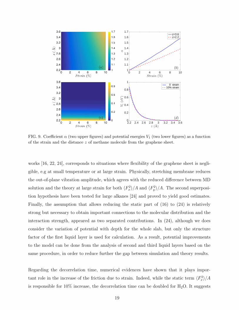
Fig. 9 represents the dependence of coefficients α and V1 in terms of the distance z of a

methane molecule from the graphene sheet. As can be seen, both strain and z can affect α

and V1, but the strain mainly contributes to the linear change of α while the potential ener-

gies coefficient V1 is very sensitive to z. The variation of V1(z) in the range, z ∈ [2.2, 3.6](A),

17

1 2 3 4 5|q| (A−1)

0.5

0.75

1

1.25

1.5

S(q)

(b) 0 strain(O)10% strain(O) 0 strain(H)10% strain(H)

1 2 3 4 5|q| (A−1)

0.5

0.75

1

1.25

1.5

S(q)

(c) H2O(O)CO2(C)CH4

FIG. 8. (a) 2D structure factor of oxygen (H2O) with 10% unilateral strain on graphene sheet. (b)

The structure factor of oxygen and hydrogen of water with different q. (c) The structure factor of

oxygen (H2O), carbon (CO2) and methane (CH4) at strain-free state.

ε q1[A−1

] q3[A−1

]0 2.950 2.950

2.5% 2.932 2.8785.0% 2.915 2.8097.5% 2.900 2.74410.0% 2.885 2.682

TABLE V. The norm of reciprocal vectors for different strains. Note that q1 = q2.

better agrees with exponential form V1(z) = 3.031 × 104 exp{−5.797z}(eV) for strain free

case and V1(z) = 2.104 × 104 exp{−5.67z}(eV) for 10% strain. It suggests that using the

representative value at z0 may not yield the best estimation. In this paper we consider the

potential form of V1 when calculating the static term in (24).

In Fig.10, we can find that the static forces 〈F 2x 〉/A, 〈F 2

y 〉/A, and the decorrelation time

depend on the strain. It is noted that the spherical molecules (CH4) are less sensitive to the

unilateral strain, which agrees with the friction results shown in Fig. 6. The variation of

those quantities for H2O and CO2 is much more significant. The theoretical results from (24)

have well predicted the variation trend and the value of 〈F 2x 〉/A with strain. For 〈F 2

y 〉/A,

there are still difference between theoretical and simulation results. The simulation results

show slight changes of 〈F 2y 〉/A while it is more visible according to the theoretical prediction.

The discrepancies could be clearly understood from the analysis of the assumptions: i) the

use of a time independent potential energy surface obtained from static graphene ii) the

superposition hypothesis for molecules in Eq. (26) iii) the fact that we only account for the

structure factor in the first liquid layer. The first assumption, adopted in most theoretical

18

0 2 4 6 8 10Strain (%)

1

1.1

1.2

1.3

1.4

1.5

1.6

1.7

α

(b)

z=3.6z=2.2

2.2 2.4 2.6 2.8 3 3.2 3.4 3.6z (A)

0

0.2

0.4

0.6

0.8

1

V1(eV)

(d)

0 strain10% strain

FIG. 9. Coefficient α (two upper figures) and potential energies V1 (two lower figures) as a function

of the strain and the distance z of methane molecule from the graphene sheet.

works [16, 22, 24], corresponds to situations where flexibility of the graphene sheet is negli-

gible, e.g at small temperature or at large strain. Physically, stretching membrane reduces

the out-of-plane vibration amplitude, which agrees with the reduced difference between MD

solution and the theory at large strain for both 〈F 2x 〉/A and 〈F 2

y 〉/A. The second superposi-

tion hypothesis have been tested for large alkanes [24] and proved to yield good estimates.

Finally, the assumption that allows reducing the static part of (16) to (24) is relatively

strong but necessary to obtain important connections to the molecular distribution and the

interaction strength, appeared as two separated contributions. In (24), although we does

consider the variation of potential with depth for the whole slab, but only the structure

factor of the first liquid layer is used for calculation. As a result, potential improvements

to the model can be done from the analysis of second and third liquid layers based on the

same procedure, in order to reduce further the gap between simulation and theory results.

Regarding the decorrelation time, numerical evidences have shown that it plays impor-

tant role in the increase of the friction due to strain. Indeed, while the static term 〈F 2x 〉/A

is responsible for 10% increase, the decorrelation time can be doubled for H2O. It suggests

19

that the motion of molecules has been affected by the changes of the environment. From

atomistic viewpoint, the changes of lattice distances induce changes in the potential energy

landscape and the diffusion mechanism of molecules. Spherical molecules like CH4 are less

affected, but molecules like H2O and CO2 tend to have less mobility along x than along y.

0 2 4 6 8 10Strain (%)

1

1.6

2.2

2.8

3.4

4

〈F2 x〉/A

(10−

3N

2/m

2) (1a) Theo

Sim

0 2 4 6 8 10Strain (%)

1

1.6

2.2

2.8

3.4

4

〈F2 y〉/A

(10−

3N

2/m

2)

H2O

(1b) TheoSim

0 2 4 6 8 10Strain (%)

50

70

90

110

130

150

τt(fs)

(1c) τxxτ

yy

0 2 4 6 8 10Strain (%)

0.5

0.7

0.9

1.1

1.3

1.5

〈F2 x〉/A

(10−

3N

2/m

2) (2a) Theo

Sim

0 2 4 6 8 10Strain (%)

0.5

0.7

0.9

1.1

1.3

1.5

〈F2 y〉/A

(10−

3N

2/m

2)

CO2

(2b) TheoSim

0 2 4 6 8 10Strain (%)

30

50

70

90

110

130

τt(fs)

(2c) τxxτ

yy

0 2 4 6 8 10Strain (%)

0

0.1

0.2

0.3

0.4

0.5

〈F2 x〉/A

(10−

3N

2/m

2) (3a) Theo

Sim

0 2 4 6 8 10Strain (%)

0

0.1

0.2

0.3

0.4

0.5

〈F2 y〉/A

(10−

3N

2/m

2)

CH4

(3b) TheoSim

0 2 4 6 8 10Strain (%)

50

70

90

110

130

150

τt(fs)

(3c) τxxτ

yy

FIG. 10. Factorization of friction coefficient λ to 〈F 2〉/A and τt with strain on graphite ranging

from 0% to 10%

IV. CONCLUSIONS

In the present paper, we have considered the friction between different liquids and an

anisotropic surface, e.g graphene subject to anisotropic engineering strain. Due to the

changes of the lattice structure, the potential field of strained graphene has lost its six fold

symmetry and is responsible for anisotropic friction behavior between the liquid and the

surface. Depending on the molecular shape and interaction strength, the anisotropy degree

may vary from one fluid species to another. Using LAMMPS software, one can compute the

20

friction tensor via time correlation integral and access to structure via post process routine.

Simple predictive estimation is proposed from a constructed surface potential for strained

graphene.

The authors study three different liquids with distinct molecular shape, namely water,

carbon dioxide and methane. Numerical evidences show that the strain induced anisotropy

effect is significant, especially for non spherical molecules. When strain increases, the friction

and the anisotropy degree also increase. For example, the friction coefficient can rise 100%

for water and 50% for carbon dioxide at 10% strain along x. The friction ratio between two

directions increases from 1 to 1.6 for water and from 1 to 1.3 for carbon dioxide. However, for

spherical molecules like methane, the variation of friction is insignificant. Investigation on

the structure and dynamics of those liquids has revealed that the relaxation time increases

considerably with strain and contributes an important part in the increase of the friction.

The contribution of this work helps better understanding and modelling the friction be-

tween liquids and anisotropic surfaces. Those surfaces can exist naturally, for example in

the form of orthorombic crystal systems or cubic systems subject to misfit strain etc.. The

study also contributes practical aspects to answer energetic and environmental challenges,

specifically it is closely related to carbon dioxide sequestration process via Enhanced coal

bed methane recovery method.

ACKNOWLEDGMENTS

The authors Quy-Dong To and Van-Hoang Vo would like to thank program Hoa Sen

Lotus 30569SK and the organization CampusFrance for the travel support. We also thank

the Multi-Scale Modelling & Experimentation of Materials for Sustainable Construction

(LabEx MMCD) for their support in CPU-time. We thank Dr. Laurent Joly for his helpful

discussion with us.

[1] R. B. Schoch, J. Han, and P. Renaud, Rev. Mod. Phys. 80, 839 (2008).

21

[2] G. Karniadakis, A. Beskok, and N. Aluru, Microflows and nanoflows: Fundamentals and

simulation (Springer, New York, 2005).

[3] J. C. Eijkel and A. Van Den Berg, Microfluid. Nanofluid. 1, 249 (2005).

[4] C. Neto, D. R. Evans, E. Bonaccurso, H.-J. Butt, and V. S. Craig, Rep. Prog. Phys. 68, 2859

(2005).

[5] S. K. Kannam, B. Todd, J. S. Hansen, and P. J. Daivis, J. Chem. Phys. 138, 094701 (2013).

[6] P. Thompson and S. Troian, Nature 389, 360 (1997).

[7] D. Rapaport, The Art of Molecular Dynamics Simulation (Cambridge University Press, 2004).

[8] M. Allen and D. Tildesley, Computer Simulation of Liquids (Oxford University Press, 1989).

[9] D. Frenkel and B. Smit, Understanding Molecular Simulation: From Algorithms to Applica-

tions (Academic Press, 2002).

[10] D. Chandler, Introduction to Modern Statistical Mechanics (Oxford University Press, 1987).

[11] L. Bocquet and J.-L. Barrat, Phys. Rev. E 49, 3079 (1994).

[12] D. Evans and G. Morriss, Statistical mechanics of nonequilibrium liquids (Cambridge Univer-

sity Press, 2008).

[13] M. Majumder, N. Chopra, R. Andrews, and B. J. Hinds, Nature 438, 44 (2005).

[14] J. K. Holt, H. G. Park, Y. Wang, M. Stadermann, A. B. Artyukhin, C. P. Grigoropoulos,

A. Noy, and O. Bakajin, Science 312, 1034 (2006).

[15] E. Secchi, S. Marbach, A. Nigues, D. Stein, A. Siria, and L. Bocquet, Nature 537, 210 (2016).

[16] K. Falk, F. Sedlmeier, L. Joly, R. R. Netz, and L. Bocquet, Nano Lett. 10, 4067 (2010).

[17] S. K. Kannam, B. D. Todd, J. S. Hansen, and P. J. Daivis, J. Chem. Phys. 135 (2011).

[18] W. Xiong, J. Z. Liu, M. Ma, Z. Xu, J. Sheridan, and Q. Zheng, Phys. Rev. E 84, 056329

(2011).

[19] L. Bocquet and J.-L. Barrat, J. Chem. Phys. 139, 044704 (2013).

[20] R. Kubo, J. Phys. Soc. Jpn. 12, 570 (1957).

[21] M. Bazant and O. Vinogradova, J. Fluid Mech. 613, 125 (2008).

[22] J.-L. Barrat and L. Bocquet, Faraday Discuss. 112, 119 (1999).

[23] J. Hansen and I. McDonald, Theory of simple liquids (Academic Press, 2006).

[24] K. Falk, F. Sedlmeier, L. Joly, R. R. Netz, and L. Bocquet, Langmuir 40, 1426114272 (2012).

[25] S. J. Stuart, A. B. Tutein, and J. A. Harrison, J. Chem. Phys. 112, 6472 (2000).

[26] J. L. Abascal and C. Vega, J. Chem. Phys. 123, 234505 (2005).

22

[27] J.-P. Ryckaert, G. Ciccotti, and H. J. Berendsen, J. Comput. Phys. 23, 327 (1977).

[28] Z. E. Hughes, S. M. Tomasio, and T. R. Walsh, Nanoscale 6, 5438 (2014).

[29] J. G. Harris and K. H. Yung, J. Phys. Chem. 99, 12021 (1995).

[30] M. Vandamme, L. Brochard, B. Lecampion, and O. Coussy, J. Mech. Phys. Solids 58, 1489

(2010).

[31] M. G. Martin and J. I. Siepmann, J. Phys. Chem. B 102, 2569 (1998).

[32] G. Vidali, G. Ihm, H.-Y. Kim, and M. W. Cole, Surf. Sci. Rep. 12, 133 (1991).

[33] M. Rubes, J. Kysilka, P. Nachtigall, and O. Bludsky, Phys. Chem. Chem. Phys. 12, 6438

(2010).

[34] H. Xua, W. Chu, X. Huang, W. Sun, C. Jiang, and Z. Liu, Appl. Surf. Sci. 375, 196 (2016).

[35] S. Plimpton, J. Comput. Phys. 117, 1 (1995).

[36] M. A. Gonzalez and J. L. F. Abascal, J. Chem. Phys. 132 (2010).

[37] J. A. Thomas and A. J. McGaughey, Nano Lett. 8, 2788 (2008).

[38] T. G. Myers, Microfluid. Nanofluid. 10, 1141 (2011).

23