STR-839: ADDRESSING THE ISSUES OF MODAL IDENTIFICATION ...
8
RESILIENT INFRASTRUCTURE June 1–4, 2016 STR-839-1 ADDRESSING THE ISSUES OF MODAL IDENTIFICATION USING TENSOR DECOMPOSITION Peter W. Friesen Graduate Student, Lakehead University, Canada Ayan Sadhu Assistant Professor, Lakehead University, Canada ABSTRACT Modal identification has been an indispensable tool for condition assessment of critical civil infrastructure. Recently several signal processing techniques including time-frequency analysis have shown significant success in addressing wide range of challenges in modal identification of flexible structures. In a parallel development, tensor decomposition is explored as an attractive and versatile system identification tool that can use even a limited number of vibration sensors to estimate the modal parameters under ambient excitations. In this paper, the performance of tensor decomposition is evaluated for modal identification of a building model under a multitude of earthquake excitations. Keywords: Modal identification; tensor decomposition; nonstationary excitation; stationary durations; PGA; earthquake 1. INTRODUCTION As large infrastructure and building age, they may be subjected to significant seismic and climatic events that cause deterioration in structural elements. Structural health monitoring (SHM) (Doebling et al. 1996) is an important tool to help predict and reduce the risk of a failure that has the potential to cause property loss, injurers or loss of life. SHM has evolved from input-output analysis to output-only analysis, due to the large costs of equipment and feasibility of measuring inputs for large scale civil structures. Modal identification (Maia and Silva 2001) is one of the key components of SHM where useful modal parameters (like frequency and mode shapes) are extracted from vibration measurements and subsequently used for condition assessment. This paper examines the potential of tensor- decomposition based modal identification using vibration data under earthquake excitation. Time-frequency and time-scale analysis methods employing wavelet transform (Guo and Kareem 2015), Hilbert transform (Huang et al. 1998), empirical mode decomposition (EMD) (Darryll and Liming 2006; Sadhu 2015) and blind source separation (BSS) techniques (Sadhu 2013) are explored towards modal identification under nonstationary excitations. In parallel, tensor decomposition based methods (also known as parallel factor (PARAFAC) decomposition) have also garnered significant attention in the area of modal identification. In tensor decomposition methods, a covariance tensor is constructed from vibration measurements under multiple lags and is subsequently decomposed into co-variances of hidden sources using multilinear algebra tools such as alternating least squares (ALS) (Smilde et al. 2004; Mokios et al. 2006). Owing to the matricization operation among various lags, tensor decomposition-based methods are versatile and can be undertaken for both complete as well as partial measurement cases. Antoni and Chauhan (Antoni and Chauhan 2011) used alternating least squares (ALS) to solve tensor decomposition associated with modal identification using a limited number of sensors. The underdetermined source separation capability of PARAFAC decomposition was recently explored to identify the modal parameters of high-rise building (Abazarsa et al. 2013; Mcneill 2012; Abazarsa et al. 2015) and a structure equipped with tuned-mass damper (Sadhu et al. 2014) using limited sensor measurements. PARAFAC decomposition is recently integrated with wavelet packet transform (WPT) to improve the source separation capability where mode-mixing in the WPT coefficients is alleviated
Transcript of STR-839: ADDRESSING THE ISSUES OF MODAL IDENTIFICATION ...
RESILIENT INFRASTRUCTURE June 1–4, 2016
STR-839-1
ADDRESSING THE ISSUES OF MODAL IDENTIFICATION USING
TENSOR DECOMPOSITION
Peter W. Friesen
Graduate Student, Lakehead University, Canada
Ayan Sadhu
Assistant Professor, Lakehead University, Canada
ABSTRACT
Modal identification has been an indispensable tool for condition assessment of critical civil infrastructure. Recently
several signal processing techniques including time-frequency analysis have shown significant success in addressing
wide range of challenges in modal identification of flexible structures. In a parallel development, tensor decomposition
is explored as an attractive and versatile system identification tool that can use even a limited number of vibration
sensors to estimate the modal parameters under ambient excitations. In this paper, the performance of tensor
decomposition is evaluated for modal identification of a building model under a multitude of earthquake excitations.
Keywords: Modal identification; tensor decomposition; nonstationary excitation; stationary durations; PGA;
earthquake
1. INTRODUCTION
As large infrastructure and building age, they may be subjected to significant seismic and climatic events that cause
deterioration in structural elements. Structural health monitoring (SHM) (Doebling et al. 1996) is an important tool to
help predict and reduce the risk of a failure that has the potential to cause property loss, injurers or loss of life. SHM
has evolved from input-output analysis to output-only analysis, due to the large costs of equipment and feasibility of
measuring inputs for large scale civil structures. Modal identification (Maia and Silva 2001) is one of the key
components of SHM where useful modal parameters (like frequency and mode shapes) are extracted from vibration
measurements and subsequently used for condition assessment. This paper examines the potential of tensor-
decomposition based modal identification using vibration data under earthquake excitation.
Time-frequency and time-scale analysis methods employing wavelet transform (Guo and Kareem 2015), Hilbert
transform (Huang et al. 1998), empirical mode decomposition (EMD) (Darryll and Liming 2006; Sadhu 2015) and
blind source separation (BSS) techniques (Sadhu 2013) are explored towards modal identification under nonstationary
excitations. In parallel, tensor decomposition based methods (also known as parallel factor (PARAFAC)
decomposition) have also garnered significant attention in the area of modal identification. In tensor decomposition
methods, a covariance tensor is constructed from vibration measurements under multiple lags and is subsequently
decomposed into co-variances of hidden sources using multilinear algebra tools such as alternating least squares (ALS)
(Smilde et al. 2004; Mokios et al. 2006). Owing to the matricization operation among various lags, tensor
decomposition-based methods are versatile and can be undertaken for both complete as well as partial measurement
cases.
Antoni and Chauhan (Antoni and Chauhan 2011) used alternating least squares (ALS) to solve tensor decomposition
associated with modal identification using a limited number of sensors. The underdetermined source separation
capability of PARAFAC decomposition was recently explored to identify the modal parameters of high-rise building
(Abazarsa et al. 2013; Mcneill 2012; Abazarsa et al. 2015) and a structure equipped with tuned-mass damper (Sadhu
et al. 2014) using limited sensor measurements. PARAFAC decomposition is recently integrated with wavelet packet
transform (WPT) to improve the source separation capability where mode-mixing in the WPT coefficients is alleviated
STR-839-2
using PARAFAC decomposition (Sadhu et al. 2013, Sadhu et al. 2015). However, none of the above studies
investigate the performances of PARAFAC decomposition under earthquake excitation. This is the motivation of the
proposed research where the PARAFAC decomposition is studied under a wide range of nonstationary ground motions
and the resulting performances are discussed.
2. BASICS OF PARALLEL FACTOR DECOMPOSITION
Tensor representation of a higher dimensional signal enables use of multilinear algebra tools that are more powerful
than linear algebra tools. A vector is a first-order tensor, whereas a matrix is second-order tensor. In general, a p-th
order tensor is written as:
[1]
A third-order tensor is primarily decomposed into a sum of outer products of triple vectors (Bro 1997):
[2]
where “○” denotes outer product with and Here R is the number of rank-1 tensors
present in H. This is also defined as trilinear Model of H, where Each triple vector product is a rank-1
tensor, namely PARAFAC component. Eq. 2 represents the summation of R such PARAFAC components that fits
the higher order tensor H (Bro 1997; Lathauwer and Castaing 2008). The technique was introduced simultaneously in
two different independent works: canonical decomposition (CANDECOMP) (Carroll and Chang 1970) and
PARAFAC analysis (Harshman 1970). The details of this method are not repeated herein and can be found in above
references.
3. EQUIVALENCE OF MODAL IDENTIFICATION WITH PARAFAC DECOMPOSITION
Consider a linear, classically damped, and lumped-mass ns-degrees-of-freedom (DOF) dynamical system, subjected
to an excitation force, F(t).
[3]
where, x is a vector of displacement coordinates at the DOFs. M, C, and K are the mass, damping and stiffness
matrices of the multi-degree-of-freedom system. The solution to Eq. 3 can be expressed in terms of modal
superposition of vibration modes with the following matrix form:
[4]
The covariance matrix of vibration measurements x evaluated at time-lag can be written as:
[5]
where,
[6]
For any general ns-DOF dynamical model, above equation can be simplified as (Sadhu et al. 2013):
[7]
Considering the similarity between Eq. 2 and Eq. 7, it is seen that by decomposing the third order tensor Cx into ns
number of PARAFAC components (i.e., modal responses), the mixing matrix can be estimated. By using PARAFAC
decomposition of Cx, the resulting solutions yield the mixing matrix M = [m1, m2, m3, …, mns ] and the autocorrelation
STR-839-3
function Csr for r = 1, 2, 3, …, ns from which the natural frequency and damping of the individual modal responses can
be estimated.
4. NUMERICAL ILLUSTRATION
A dynamical system with 5 degree-of-freedoms is selected to demonstrate the performance of PARAFAC method
under base excitations. The natural frequencies of the model are 0.91, 3.4, 7.1, 10.7 and 12.7 Hz, respectively. The
model is subjected to a suite of ground motions and the resulting vibration responses are processed through PARAFAC
to extract the modal parameters under a wide range of nonstationary excitations. Table 1 shows six typical ground
motions selected for preliminary study along with the detailed information of peak ground acceleration (PGA) and
ground motion duration (T). The extent of non-stationarity is characterized by the ratio of stationary duration (Ts)
(Trifunac and Brady 1975) and T. Ts (Trifunac and Brady 1975) may be computed using the time interval containing
the energy envelope between 5 and 95 percent of the total energy of an earthquake. An earthquake is considered
stationary when a majority of the energy is released between 5 and 95 percent of the total earthquakes duration. On
the other hand, when this ratio attains lower value say, ≤ 0.3, the earthquake (i.e., NR and PF) is extremely non-
stationary in nature in time-domain.
Table 1: Details of example ground motions
Earthquake PGA (g) T (s) Ts/T
El Centro (EC), 1940 0.004 50.0 0.50
Northridge (NR), 1994 0.009 60.0 0.12
Imperial Valley (IV), 1940
Kern County (KC), 1952
Parkfield (PF), 1966
San Fernando (SF), 1971
0.36
0.16
0.37
0.02
53.8
54.4
44.0
68.7
0.47
0.63
0.21
0.67
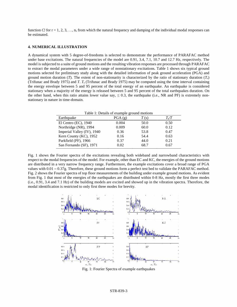
Fig. 1 shows the Fourier spectra of the excitations revealing both wideband and narrowband characteristics with
respect to the modal frequencies of the model. For example, other than EC and KC, the energies of the ground motions
are distributed in a very narrow frequency range. Furthermore, the example excitations cover a broad range of PGA
values with 0.01 – 0.37g. Therefore, these ground motions form a perfect test bed to validate the PARAFAC method.
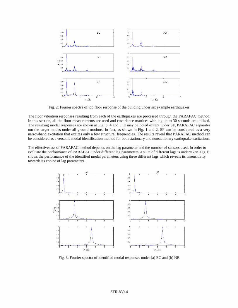
Fig. 2 shows the Fourier spectra of top floor measurements of the building under example ground motions. As evident
from Fig. 1 that most of the energies of the earthquakes are distributed within 0-8 Hz, mostly the first three modes
(i.e., 0.91, 3.4 and 7.1 Hz) of the building models are excited and showed up in the vibration spectra. Therefore, the
modal identification is restricted to only first three modes for brevity.
Fig. 1: Fourier Spectra of example earthquakes
STR-839-4
Fig. 2: Fourier spectra of top floor response of the building under six example earthquakes
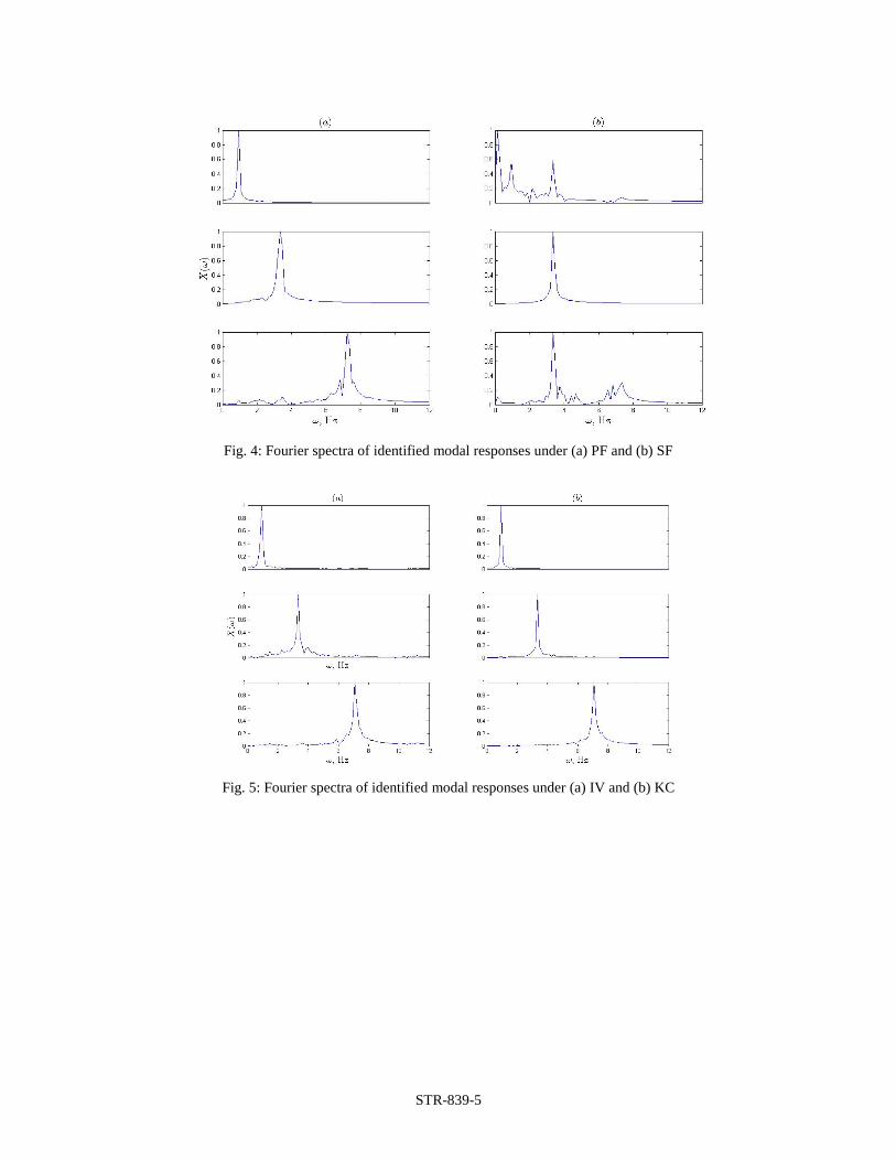
The floor vibration responses resulting from each of the earthquakes are processed through the PARAFAC method.
In this section, all the floor measurements are used and covariance matrices with lag up to 30 seconds are utilized.
The resulting modal responses are shown in Fig. 3, 4 and 5. It may be noted except under SF, PARAFAC separates
out the target modes under all ground motions. In fact, as shown in Fig. 1 and 2, SF can be considered as a very
narrowband excitation that excites only a few structural frequencies. The results reveal that PARAFAC method can
be considered as a versatile modal identification method for both stationary and nonstationary earthquake excitations.
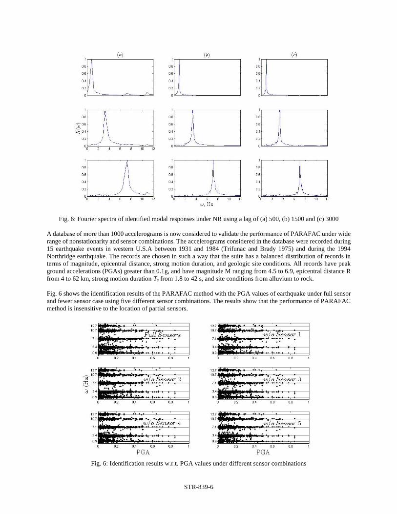
The effectiveness of PARAFAC method depends on the lag parameter and the number of sensors used. In order to
evaluate the performance of PARAFAC under different lag parameters, a suite of different lags is undertaken. Fig. 6
shows the performance of the identified modal parameters using three different lags which reveals its insensitivity
towards its choice of lag parameters.
Fig. 3: Fourier spectra of identified modal responses under (a) EC and (b) NR
STR-839-5
Fig. 4: Fourier spectra of identified modal responses under (a) PF and (b) SF
Fig. 5: Fourier spectra of identified modal responses under (a) IV and (b) KC
STR-839-6
Fig. 6: Fourier spectra of identified modal responses under NR using a lag of (a) 500, (b) 1500 and (c) 3000
A database of more than 1000 accelerograms is now considered to validate the performance of PARAFAC under wide
range of nonstationarity and sensor combinations. The accelerograms considered in the database were recorded during
15 earthquake events in western U.S.A between 1931 and 1984 (Trifunac and Brady 1975) and during the 1994
Northridge earthquake. The records are chosen in such a way that the suite has a balanced distribution of records in
terms of magnitude, epicentral distance, strong motion duration, and geologic site conditions. All records have peak
ground accelerations (PGAs) greater than 0.1g, and have magnitude M ranging from 4.5 to 6.9, epicentral distance R
from 4 to 62 km, strong motion duration Ts from 1.8 to 42 s, and site conditions from alluvium to rock.
Fig. 6 shows the identification results of the PARAFAC method with the PGA values of earthquake under full sensor
and fewer sensor case using five different sensor combinations. The results show that the performance of PARAFAC
method is insensitive to the location of partial sensors.
Fig. 6: Identification results w.r.t. PGA values under different sensor combinations
STR-839-7
5. CONCLUSIONS
In this paper, PARAFAC decomposition is explored as a possible tool for modal identification under earthquake
excitations. The method is validated using a suite of ground motions covering wide range of nonstationary
characteristics. The effects of lag parameter and rank order selection of PARAFAC decomposition are also
investigated for a numerical model under complete and limited sensor measurements.
ACKNOWLEDGEMENT
The authors gratefully acknowledge the funding provided by the Natural Sciences Engineering Research Council of
Canada (NSERC) through the second author's Discovery Grant program to undertake this work.
REFERENCES
Abazarsa, F., Ghahari, S. F., Nateghi, F., and Taciroglu, E. (2013). “Response-only modal identification of structures
using limited sensors.” Structural Control and Health Monitoring, Wiley, 20(6), 987-1006.
Abazarsa, F., Nateghi, F., Ghahari, S. F., and Taciroglu, E. (2015). “Extended blind modal identification technique
for nonstationary excitations and its verification and validation.” Journal of Engineering Mechanics, ASCE, 1-19.
Antoni, J. and Chauhan, S. (2011). “An alternating least squares based blind source separation algorithm for
operational modal analysis.” Proceedings of the 29th IMAC, Jacksonville (FL), USA.
Bro, R. (1997). “Parafac: Tutorial and applications.” Chemomemcs and Intelligent Laboratory Systems, San Antonio,
Texas, 38, 149-171.
Carroll, J. D. and Chang, J. J. (1970). Analysis of individual differences in multidimensional scaling via an n-way
generalization of Eckart-young decomposition." Psychometrika, 35, 283-319.
Darryll, P. and Liming, S. (2006). “Structural health monitoring using empirical mode decomposition and the Hilbert
phase.” Journal of Sound and Vibration, 294(1-2), 97-124.
Doebling, S., Farrar, C., Prime, M., and Shevitz, D. (1996). “Damage identification and health monitoring of structural
and mechanical systems from changes in their vibration characteristics: a literature review.” Technical Report LA-
13070-MS, Los Alamos National Laboratory, Los Alamos, NM.
Guo, Y. and Kareem, A. (2015). “System identification through nonstationary response: wavelet and transformed
singular value decomposition-based approach.” Journal of Engineering Mechanics, ASCE, 141(7).
Harshman, R. A. (1970). “Foundations of the PARAFACprocedure: Models and conditions for an explanatory
multi-model factor analysis.” UCLA working papers in Phonetics, 16, 1-84.
Huang et al., N. E. (1998). “The empirical mode decomposition for the Hilbert spectrum for nonlinear and non-
stationary time series analysis.” Proceedings of Royal Society of London Series, 903-95.
Lathauwer, L. D. and Castaing, J. (2008). “Blind identification of underdetermined mixtures by simultaneous matrix
diagonalization.” IEEE Transactions on Signal Processing, 56(3), 1096-1105.
Maia, N. M. M. and Silva, J. M. M. (2001). “Modal analysis identification techniques.” Philosophical transactions of
the royal society, 359(1778), 29-40.
Mcneill, S. I. (2012). “Extending blind modal identification to the underdetermined case for ambient vibration.”
ASME 2012 International Mechanical Engineering Congress and Exposition, Houston, Texas, USA, November,
2012, 241-252.
STR-839-8
Mokios, K., Sidiropoulos, N. D., and Potamianos, A. (2006). “Blind speech separation using PARAFACanalysis
and integer least squares.” Proceedings of ICASSP'06, 5, 73-76.
Sadhu, A. (2013). “Decentralized ambient modal identification of structures.” PhD Thesis, Department of Civil and
Environmental Engineering, University of Waterloo, Canada, 1-180.
Sadhu, A. (2015). “An integrated multivariate empirical mode decomposition method towards modal identification of
structures.” Journal of Vibration and Control, DOI: 10.1177/1077546315621207
Sadhu, A., Goldack, A., and Narasimhan, S. (2015). “Ambient modal identification using multi-rank parallel factor
decomposition.” Structural Control and Health Monitoring, Wiley, 22(4), 595-614.
Sadhu, A., Hazra, B., and Narasimhan, S. (2013). “Decentralized modal identification of structures using parallel
factor decomposition and sparse blind source separation.” Mechanical Systems and Signal Processing, Elsevier,
41(1-2), 396-419.
Sadhu, A., Hazra, B., and Narasimhan, S. (2014). “Ambient modal identification of structures equipped with tuned
mass dampers using parallel factor blind source separation.” Smart Structures and Systems, Techno press, 13(2),
257-280.
Sadhu, A., Hazra, B., Narasimhan, S., and Pandey, M. D. (2011). “Decentralized modal identification using sparse
blind source separation.” Smart Materials and Structures, IOP, 20(12), 125009.
Smilde, A., Bro, R., and Geladi, P. (2004). Multi-way Analysis with Applications in the Chemical Sciences. John
Wiley and Sons, Ltd, West Sussex, UK.
Trifunac, M. and Brady, A. (1975). “A study on the duration of strong earthquake ground motion.” Bulletin of the
Seismological Society of America, 65(3), 581-626.