Stock market volatility: friend or foe?

1

Stock market volatility: friend or foe?

Michael Dempseya, Abeyratna Gunasekarageb, Thanh Tan Truongc

A version of the paper subsequently published by

Accounting and Finance (2020, vol. 60 (4), p. 3477-3492)

a Faculty of Finance and Banking, Ton Duc Thang University, Ho Chi Minh City, Vietnam.

b Monash Business School, Monash University, Melbourne, Australia.

c School of Economics, Finance and Marketing, RMIT University, Melbourne, Australia.

Electronic copy available at: https://ssrn.com/abstract=3750194

2

Stock market volatility: friend or foe?

Abstract

Although a good deal of research effort has been allocated to understanding the time-series

volatility of stock returns – as both market (or systematic) volatility and idiosyncratic (or non-

systematic) volatility – the relationship of such volatility with cross-sectional volatility or

dispersion of outcomes is sparse. Nevertheless, the quest to understand one must involve the quest

to understand the other. In this paper, we investigate the dynamic of the dispersion of return

outcomes in generating a portfolio’s expected return outcome. We find that changes in the level of

cross-sectional volatility have highly significant implications for portfolio performances and the

notion of risk.

Key words: Investment horizon; Market return; Market; Risk; Stock performance; Volatility

JEL classification: G10, G11, G12


3

1. Introduction

Although a good deal of attention has been accorded to stock volatility as the time-variation of

stock returns, much less attention has been accorded to their cross-sectional variation, which is to

say, the dispersion, of stock returns. Nevertheless, the two variations are related. In which case, a

satisfactory understanding of one requires an understanding of the other. The present paper

highlights how a dispersion of return outcomes, of its statistical nature, implies a relation between

inter-temporal volatility and higher returns. In this case, the higher portfolio returns so generated

are not the outcome of investors “setting prices” in accordance with their required expectations in

relation to risk (the fundamental assumption of academic asset pricing), but, rather, are

forthcoming as a mathematical or statistical consequence of the risky nature of growth itself. Our

results have implications for professional investment strategies as well as for a fuller understanding

of risk and volatility.

Campbell, Lettau and Malkiel (2001) have reported how a higher level of inter-temporal

sector volatility and a reduction in cross-sector correlations contribute to an increased cross-

sectional dispersion of outcomes (Ankrim and Ding, 2002). Cross-sectional dispersion is thereby

related to inter-temporal firm volatility. In a similar vein, Solnik and Roulet (2000) show how the

cross-sectional dispersion of stockmarket returns is related to global levels of inter-temporal

stockmarket correlations. Consistently, for Australian stocks, Alaganar and Whiteoak (2004) find

that the cross-sectional volatility of stock returns is associated with increases in inter-temporal

sector volatility and reductions in cross-sector correlations. As an outcome of a bootstrapping

exercise whereby historical returns are assumed to represent unbiased estimates of the range of

market outcomes over investment horizons, Fama and French (2018) have also demonstrated a

relationship between market performance and the cross-sectional dispersion of outcomes.


4

Consistent with the above, we advance a statistical model that recognizes that the

individual time-series volatility of asset returns and the cross-sectional volatility of their returns

combined are necessarily related.1 Consistent with the model, we determine that - as opposed to

market outcomes representing the outcome of investors setting prices (so as to generate higher

expected outcomes) in response to higher volatility - the dynamic of higher market rewards can be

related to the merely statistical outcome of volatility. The idea that “excess growth” can emerge

as the statistical outcome of stock return variance is not new (Fernholz and Shay, 1982; Booth and

Fama, 1992). Nevertheless, the impact of such papers to date appears to have been marginal. We

demonstrate the proposed statistical model in the context of both the US stockmarket (over long-

term investment periods), as well as in the context of historical Australian share prices (over

monthly investment periods).

To these ends, the rest of the paper is as follows. The following section clarifies the

fundamental statistical model applied to asset growth. Section 3 applies the model to the long-term

performances of the US stockmarket and Section 4 applies the model to the monthly stockmarket

performances for Australian shares. Section 5 concludes.

2. The model

When we apply a randomly selected exponential growth rate from a normal distribution with mean

per period with standard deviation σ about such mean, to an asset price $P0 at the commencement

1 We can recognize that in the particular case that asset returns are perfectly uncorrelated, but share an identical time-

series volatility, the time-series volatility and the cross-sectional volatility of the asset individual returns are one and

the same.


5

of a period, we can represent the (unknown) outcome asset price at the end of N periods, $𝑃𝑡+𝑁,

as

$𝑃𝑡+𝑁 = $𝑃𝑡𝑒𝑁𝜇+√𝑁𝑍σ (1)

where Z represents a selection from -∞ to +∞ with the probability of selection determined by the

“unit normal” distribution (with mean zero and standard deviation equal to one).

The assumption that stockmarket growth might be modeled at least approximately by such

a process is, to some extent, justified by the evidence of past stock price performance. In addition,

we have the argument of the “central limit theorem” (the “theorem of large numbers”) that reveals

that even when exponential growth rates are not normally distributed in the short-term, provided

the outcomes over successive periods are drawn independently from the same distribution, the

outcome longer-term growth rate over a large number of N sub-time intervals will tend to be a

normal distribution with mean (μ) and standard deviation (σ) determined as

𝜇 = 𝑁𝜇∗

(2)

and

σ = (√𝑁)σ∗ (3)

where μ* is the mean of the exponential growth rates with standard deviation, σ*, over each sub-

time interval (for example, Fama, 1976).

The exponential growth rate, R, that provides the “expected” (which is to say, probability-

weighted) price outcome at the end of the period, is defined by


6

$𝑃0𝑒𝑅 ≡ 𝑡ℎ𝑒 "expected" 𝑝𝑟𝑖𝑐𝑒 𝑜𝑢𝑡𝑐𝑜𝑚𝑒 𝑜𝑓𝑖𝑛𝑣𝑒𝑠𝑡𝑚𝑒𝑛𝑡 $𝑃0 𝑓𝑜𝑟 𝑎 𝑠𝑖𝑛𝑔𝑙𝑒 𝑝𝑒𝑟𝑖𝑜𝑑,

which is to say as

𝑅 ≡ 𝐿𝑛[𝑒𝑥𝑝𝑒𝑐𝑡𝑒𝑑 𝑤𝑒𝑎𝑙𝑡ℎ 𝑜𝑢𝑡𝑐𝑜𝑚𝑒 𝑜𝑓 𝑖𝑛𝑣𝑒𝑠𝑡𝑖𝑛𝑔 $1 𝑓𝑜𝑟 𝑎 𝑠𝑖𝑛𝑔𝑙𝑒 𝑝𝑒𝑟𝑖𝑜𝑑] (4)

where Ln represents the natural log function. As a statistical outcome, R is determined as

𝑅 = 𝜇 +1

2σ2 (5)

where the asset or portfolio volatility (σ) in Equation (5) may comprise both market and

idiosyncratic volatility.2

Investors, of course, assess stock prices not in terms of their potential exponential growth

characteristics, but in terms of their “expected discrete periodic return”, by which we mean the

expected percentage increase in wealth generated over some discrete period (a month, a year).

Such return (r) is expressed:

2 As a point of interest, Equation (5) is applied in the Black-Scholes model. Thus, the assumption of “risk neutrality”

leads to the risk-free rate, 𝑟𝑓 = 𝜇 +1

2σ2, so that is then replaced by 𝑟𝑓 −

1

2σ2 in the model’s familiar expressions.

See, for example, Chapter 8 in the student textbook: “Financial Risk Management and Derivative Instruments” (2021)

by Michael Dempsey (Routledge, Oxon, England).


7

𝑟 ≡[𝑒𝑥𝑝𝑒𝑐𝑡𝑒𝑑 𝑝𝑟𝑖𝑐𝑒 𝑜𝑢𝑡𝑐𝑜𝑚𝑒 𝑜𝑓 𝑖𝑛𝑣𝑒𝑠𝑡𝑚𝑒𝑛𝑡 $𝑃0 𝑓𝑜𝑟 𝑎 𝑠𝑖𝑛𝑔𝑙𝑒 𝑝𝑒𝑟𝑖𝑜𝑑− $𝑃0]

$𝑃0 (6)

where $P0 is the investment at commencement of the investment period. In order to generalize the

relationship between the above periodic return – which is to say, the “surface” return that market

participants seek to measure – and the “sub-surface” continuously applied parameters µ and σ

(which generate the surface periodic return), we observe that the expected price outcome can be

expressed equally as either

$𝑃0𝑒𝑅 (with the definition of Equation (4))

or as

$𝑃0(1 + 𝑟) (with the definition of Equation (6)).

Thus, we have

𝑟 = 𝑒𝑅 − 1 (7)

which with Equation 5 provides

𝑟 = 𝑒𝜇+½σ2− 1 (8)

so that provided R is a “smallish fraction” (allowing that we are considering rates on an annual


8

basis, or less), we can express eR as approximately 1 + R, so that we have

𝑟 𝑎𝑝𝑝𝑟𝑜𝑥𝑖𝑚𝑎𝑡𝑒𝑙𝑦 = 𝑅 = 𝜇 +1

2σ2 (9)

Since ½σ2 is necessarily positive, Equation (9) is the statement that the volatility of returns

(σ) in an exponential growth process acts to increase the expected (probability-weighted) periodic

return.3 Nevertheless, the theoretical return outcome remains probabilistic. That is to say, although

the expected or probability-weighted wealth outcome is increased by outcome volatility (σ) as

Equation (9), the ultimate outcome is nevertheless a single outcome return from a distribution

made wider (more risky) by virtue of the self-same return volatility (σ).4

An additional dynamic of volatility emerges when we consider Equation (9) applied to the

individual assets that comprise a portfolio. To see this, we must consider how the individual returns

of assets generated by volatility contribute to an overall portfolio return, as well as how the

individual asset volatilities combine to determine the overall volatility of the portfolio of such

assets. Thus, firstly, we observe that the discrete expected return for a portfolio of remains as the

asset value weighted-average of the expected returns of the individual assets in the portfolio assets

(notwithstanding that the individual asset returns are augmented by asset volatility). Secondly, we

observe that the market volatility of the portfolio returns is also the asset value weighted-average

of the market volatilities of the individual assets. Thirdly, however, we observe that the

3 This observation is in accord with findings to date. For example, Malkiel and Xu (1997), Goyal and Santa-Clara

(2003) and Fu (2009) report that idiosyncratic volatility is significantly and positively related to stock returns in the

US. Findings by Ang, Hoddrick, Xing and Zhang (2006) who report a negative relationship between lagged

idiosyncratic volatility and future average returns are often referenced as contradicting the findings of a positive

relation. Nevertheless, their findings may be interpreted in relation to the behavioral role of idiosyncratic volatility as

the “messenger” of declining market confidence with consequent lower asset prices. 4 The implications of Equation 9 for investments and portfolio construction are developed in the student textbook:

“Investment Analysis: An Introduction to Portfolio Theory and Management” (2020) by Michael Dempsey

(Routledge, Oxon, England).


9

idiosyncratic volatility of the portfolio is necessarily less than the asset value weighted-average of

the idiosyncratic volatilities of the individual assets, and approaches zero with many assets. We

therefore observe that with independently performing assets, we retain the asset value weighted

return generated by the individual asset volatilities (which benefits from the individual asset

volatilities), while simultaneously reducing the portfolio volatility of the assets combined.

In the following section, we demonstrate the contribution of market volatility to the

expected return of the market portfolio over long-term periods. In the section thereafter, we

observe the impact of individual asset volatilities (allowing both market and idiosyncratic

volatility) on portfolio outcomes.

3. The long-term implications of the cross-sectional dispersion of outcomes: the results

of Fama and French (2018)

Fama and French (2018) examine the average stockmarket returns (above the T-bill rate) for a

range of investment time horizons. The results are the outcome of a bootstrapping exercise

whereby the monthly returns for the stockmarket period 1963-2016 are treated as the population

of return possibilities from which 100,000 trials are drawn randomly with associated T-bill returns.

The results are presented in the first numerical column of Table 1 (annualized in parentheses).

Thus, we observe a dramatic increase in the “expected” (average) premium return, RET (over the

T-bill rate), as the distributions become more disperse with a longer investment time horizon. As

observed by Fama and French (2018), a contributing factor to the higher values for the equity

premiums is the increasing skew to higher outcome returns combined with a higher kurtosis of

both higher positive and negative outcome returns than is predicted by a normal distribution. The


10

second numerical column is the standard deviation (SD) of the returns over the same investment

time horizon as reported by Fama and French.

Table 1 about here.

The third and fourth columns impose a “best fit” normal distribution on the Fama and

French data by transposing the expected return (RET) and standard deviation (SD) of the Fama and

French outcomes to the expected return (μ) and the standard deviation (σ) consistent with a normal

distribution of exponential growth rates. Thus, in numerical column 3 of the table, we apply the

formula5:

σ2 = 𝐿𝑛 [1 +𝑆𝐷2

(1+𝑅𝐸𝑇)2] (10)

where the expected return (RET) and standard deviation of returns (SD), respectively, are as

numerical columns 1 and 2. For example, for a 10-year investment horizon, we have the expected

return (RET) = 133% and standard deviation (SD) = 149%, so that

σ2 = 𝐿𝑛 [1 +1.492

(1+1.33)2] = 0.343,

which determines σ = √0.343 = 0.585 (58.5%), as in the table, or as 0.585/√10 = 0.185 (18.5%)

annualized. We note the reasonably consistent value of the annualized standard deviation so

5 See the Appendix of Mehra (2003) for a proof of Equation (10).


11

calculated (average = 17.5% per year), which is consistent with returns generated over successive

periods by a normal distribution. With σ so defined, we transpose the Fama and French expected

return (RET) as the mean exponential growth rate (μ) assuming a normal distribution (consistent

with Equation (5) as

𝜇 = 𝐿𝑛(1 + 𝑅𝐸𝑇) −1

2σ2 (11)

as in the fourth numerical column of the table. As confirmation, column 5 re-constructs the Fama

and French expected (average) returns of column 1 assuming a normal distribution of outcomes

with μ and σ as in columns 3 and 4.

With a view to revealing the impact of skew and kurtosis with an increasing investment

horizon, numerical column 6 provides the expected (average) returns assuming a normal

distribution with μ and σ as their one-year values (μ = 5.5% per annum and σ = 15.8% per annum,

first numerical row), which is to say, imposing skew and kurtosis equal to zero following a one-

year investment horizon. The implications of skew and kurtosis appear to be highly significant.

Thus, we observe that with an increasing investment time horizon, the skew to a higher distributed

outcome return has a compounding effect, with the outcome that the expected (average) outcomes

calculated by Fama and French (2018) are increasingly higher than the fixed annualized rate

(7.0%) predicted by a normal distribution. After 10-years, the Fama and French annualized

expected (average) return outcome is 8.8% compared with 7.0% predicted by a normal

distribution; and after 30 years, the Fama and French annualized return is 10.9% compared with

7.0% predicted by a normal distribution (numerical columns 1 and 6).


12

The final column represents the outcome of maintaining μ = 5.5% per annum while setting

σ = 0, which is to say, assuming a normal distribution with skew, kurtosis and volatility each equal

to zero. The column reveals a consistent 1.35% return per annum (7.0% - 5.65%) as the outcome

of market volatility.

In summary, the table reveals that stock volatility combined with a positive skew or tilt (to

the higher returns) and kurtosis leads statistically to increasingly higher return outcomes with

longer investment horizons than is predicted by risk-free growth. The overall addition to the

expected return over a 10-year period as an outcome of diverse return outcomes appears to be close

to 3.15% annualized (8.8%-5.65%), and over a 30-year period, closer to 5.25% annualized (10.9%-

5.65%).

In Table 2, we present the outcomes calculated by Fama and French from their 1963-2016

returns (the F&F columns) for (a) the probability of underscoring the T-bill rate over a range of

investment time horizons (as “Neg”) and (b) the dispersion of the equity premium returns at the

5% and 95% probability boundaries (as 5% percentile and 95% percentile respectively). The table

shows how with an increasingly longer investment horizon, excess returns become more disperse

but move faster to the right. We also observe that as the return horizon increases, the probability

of underscoring the T-bill rate decreases monotonically. In addition, we observe that the 95%

percentile increases monotonically, whereas the 5% percentile becomes more negative (indicating

the loss at this probability) as the investment horizon increases – but, intriguingly, only to a point

– as somewhere above the 10-year investment horizon, the loss at this probability actually begins

to decrease before turning positive. At a 30-year investment horizon, the anticipated outcome at

the lower 5% percentile is a positive 37% return.


13

Table 2 about here.

Retaining a normal distribution with μ and σ as their one-year values (μ = 5.5% per annum

and σ = 15.8% per annum) for each investment time horizon, we recalculate the outcomes for the

5% and 95% probability boundaries, as well as the probability that the premium is less than zero.

The outcomes are as presented alongside those of Fama and French in Table 2. In the table, we

observe that the normal distribution has preserved the essential features noted by Fama and French,

even the observation that the 5% percentile becomes more negative (a greater loss at this

probability) as the investment horizon increases, but only to a point, beyond which the loss at this

probability actually begins to decrease. Thus, consistent with the Fama and French results, at a 30-

year investment horizon, the predictions have been transformed from a negative return outcome to

a (25%) gain. For the 95% percentile, the outcomes increase monotonically.

The essential dynamic underlying the outcomes for a normal distribution is that whereas

the mean µ of the outcome returns increases linearly with time, the standard deviation σ of the

return outcomes increases only as the square-root of time (Equations 2 and 3), so that with

increasing investment horizon, the impact of increasing µ eventually dominates the impact of

increasing σ. Notwithstanding, in the absence of skew and kurtosis, the outcome returns with an

increasing investment horizon for a normal distribution, fall increasingly behind those of Fama

and French. As revealed in Table 1, at the 20-year investment horizon, the normal distribution

(column 6) predicts only ½ of the return indicated by the empirically-based result of Fama and

French (column 1); and at the 30-year investment horizon, the normal distribution predicts only ⅓

of the return indicated by Fama and French.


14

The above observations motivate us to examine the empirical relation between the inter-

temporal monthly return performance for a portfolio of stocks in relation to the cross-sectional

dispersion of the portfolio’s stock returns, to which we turn in the following section.

4. The implications of monthly cross-sectional dispersion of outcomes: the evidence of

Australian data

We avail of the data from Datastream for the Australian Securities Exchange (ASX) monthly stock

prices for the period January 2006 – December 2017. We calculate the monthly discrete return

𝑟𝑖,𝑡 =$𝑃𝑖,𝑡

$𝑃𝑖,𝑡−1− 1 and monthly exponential growth rate 𝑔𝑖,𝑡 = 𝑙𝑛

$𝑃𝑖,𝑡

$𝑃𝑖,𝑡−1 for each individual stock,

where $𝑃𝑖,𝑡 is the price of stock i at the end of month t. Thereafter, for each calendar month, t, we

calculate the following:

(a) the discrete monthly return for portfolio P represented by the average of the individual

monthly discrete returns of all the stocks in the portfolio:

𝑅𝐸𝑇𝑃,𝑡 =1

𝑛∑ 𝑟𝑖,𝑡

𝑛

𝑖=1,

(b) the average monthly exponential growth rate of the stocks in portfolio P as:

𝜇𝑃,𝑡 =1

𝑛∑ 𝑔𝑖,𝑡

𝑛

𝑖=1,

(c) the actual exponential growth rate for portfolio P:

𝑅𝑃,𝑡 = 𝑙𝑛$𝑉𝑃,𝑡

$𝑉𝑃,𝑡−1 ,

(where $𝑉𝑃,𝑡 is the dollar value of the portfolio at the end of month t),

(d) the cross-sectional dispersion of the discrete returns for portfolio P represented by the

standard deviation of the discrete returns of all the stocks in the portfolio:

𝑆𝐷𝑃,𝑡 = √∑ (𝑟𝑖,𝑡−𝑅𝐸𝑇𝑃,𝑡)2𝑛

𝑖=1

𝑛−1,


15

(e) the cross-sectional dispersion of the exponential growth rates for portfolio P represented

by the standard deviation of the exponential growth rates of all the stocks in the portfolio:

𝜎𝑃,𝑡 = √∑ (𝑔𝑖,𝑡−𝜇𝑃,𝑡)2𝑛

𝑖=1

𝑛−1, and

(f) the time-series volatility of portfolio discrete returns represented by the standard

deviation of portfolio discrete returns for the most recent twelve months:

𝑉𝑂𝐿𝑃,𝑡 = √∑ (𝑅𝐸𝑇𝑃,𝑡−𝑅𝐸𝑇̅̅ ̅̅ ̅̅ 𝑃)212

𝑡=1

11,

where 𝑅𝐸𝑇̅̅ ̅̅ ̅̅𝑃 is the average monthly discrete return for portfolio P in the twelve-month

period.6

To begin, we measure both the time-series volatility and cross-sectional standard deviation

for a portfolio of (1) “all” stocks, (2) stocks of “large” firms and (3) stocks of “small” firms.

“Large” firms are the largest 25% of firms by market capitalization in the ASX, and “small” firms

are the remaining 75% of firms in the sample for each month. Table 3 presents the average time-

series monthly volatility (VOLP,t) of the stock discrete returns, and the average monthly cross-

sectional standard deviation (SDP,t) of the stock discrete returns for the above three portfolios. We

observe that a portfolio of stocks of small firms has both a higher time-series volatility (VOL) and

a higher cross-sectional dispersion (SD) compared with stocks of large companies and the entire

market.

Table 3 about here.

6 We focus on the time-series volatility of discrete returns (as opposed to exponential returns) because the concept of

stockmarket “risk” in the literature is generally identified as the time-series volatility of discrete returns.


16

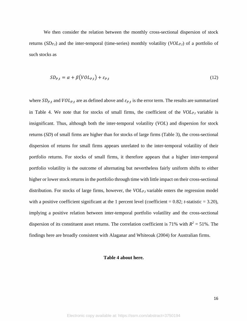
We then consider the relation between the monthly cross-sectional dispersion of stock

returns (SDP,t) and the inter-temporal (time-series) monthly volatility (VOLP,t) of a portfolio of

such stocks as

𝑆𝐷𝑃,𝑡 = 𝛼 + 𝛽(𝑉𝑂𝐿𝑃,𝑡) + 𝜀𝑃,𝑡 (12)

where 𝑆𝐷𝑃,𝑡 and 𝑉𝑂𝐿𝑃,𝑡 are as defined above and 𝜀𝑃,𝑡 is the error term. The results are summarized

in Table 4. We note that for stocks of small firms, the coefficient of the VOLP,t variable is

insignificant. Thus, although both the inter-temporal volatility (VOL) and dispersion for stock

returns (SD) of small firms are higher than for stocks of large firms (Table 3), the cross-sectional

dispersion of returns for small firms appears unrelated to the inter-temporal volatility of their

portfolio returns. For stocks of small firms, it therefore appears that a higher inter-temporal

portfolio volatility is the outcome of alternating but nevertheless fairly uniform shifts to either

higher or lower stock returns in the portfolio through time with little impact on their cross-sectional

distribution. For stocks of large firms, however, the VOLP,t variable enters the regression model

with a positive coefficient significant at the 1 percent level (coefficient = 0.82; t-statistic = 3.20),

implying a positive relation between inter-temporal portfolio volatility and the cross-sectional

dispersion of its constituent asset returns. The correlation coefficient is 71% with R2 = 51%. The

findings here are broadly consistent with Alaganar and Whiteoak (2004) for Australian firms.

Table 4 about here.


17

We wish to test the contribution of individual stock volatilities to a portfolio’s overall

return as predicted by Equation (5). To this end, the actual monthly exponential return for a

portfolio, RP,t = 𝑙𝑛$𝑉𝑃,𝑡

$𝑉𝑃,𝑡−1, as above, over and above the mean monthly exponential return for the

stocks in the portfolio, P,t, as RP,t - P,t, is regressed against the dispersion of the portfolio’s

exponential returns in that particular month (σP,t), as

𝑅𝑃,𝑡 − 𝜇𝑃,𝑡 = 𝛼 + 𝛾 (1

2σ𝑃,𝑡

2 ) + 𝜀𝑃,𝑡 (13)

The results are summarized in Table 5. For all stocks, as well as for stocks of both large

and small firms separately, the findings reveal a clear positive relation between the average inter-

temporal return for a portfolio over and above the median of the portfolio’s individual stock

returns, as R - μ, and the cross-sectional dispersion of the stock returns as ½2 for the period. For

small firms, we observe an effective alignment of outcomes with the statistical relation of Equation

(5): correlation = 75% and R2 = 56%, and a coefficient on ½2 = 0.98 (t-statistic 13.47) with an

insignificant intercept. For large firms, we have an even greater correlation = 88% and R2 = 77%,

with a coefficient on ½2 = 0.39 (t-statistic 21.68) with a significant intercept = 0.0042 (t-statistic

14.53) together accounting for the robust correlation and R2.

Table 5 about here.

With an average annual cross-sectional standard deviation (σ) for the exponential returns

over the period of study as 21.8%, Equation (5) predicts that the return generated by such standard


18

deviation is ½(0.218)2 or 2.4% per annum. For stocks of larger firms, the annual standard

deviations are lower, at an average 13.6%, implying a contribution to performance as ½(0.136)2

or 0.9% per annum; while for stocks of smaller firms, the standard deviations are higher, at an

average 23.7%, implying a contribution to performance as ½(0.237)2 or 2.8% per annum. The

outcomes appear broadly consistent with the result derived for US stocks in the previous section,

namely a 1.35% return per annum (7.0% - 5.65%) as the outcome of market volatility.

As for the US findings in the previous section, the impact of volatility is significantly

augmented by skew and kurtosis. Thus, the average median monthly returns (of $𝑃𝑡

$𝑃𝑡−1− 1) for the

stocks are close to zero for all firms, large firms and small firms, whereas the average monthly

mean returns (of $𝑃𝑡

$𝑃𝑡−1− 1) are, respectively, 1.3% per month (all firms), 0.27% per month (large

firms) and 1.6% per month (small firms). In other words, the positive performance of stockmarket

returns is dependent on the volatility and outcome dispersion of the return outcomes, whereby the

mean return of the stock returns exceeds their median return. Conclusion: the investor needs

volatility!

Finally, we repeated the regression Equation (13) by restricting the sample in each month

to (a) stocks with positive outcome returns only and (b) stocks with negative outcome returns only.

The results are displayed in Table 6. For positive outcome returns, the table reveals the additional

contribution of dispersion (σ) to the overall return R in that month as a coefficient = 2.0 on ½2,

while for the negative returns sample, the additional contribution of dispersion (σ) to the return R

is a coefficient = 0.45. Thus, although the benefits of cross-sectional dispersion are most

effectively materialized during up-market periods, the effect remains overall positive even in

declining markets.


19

Table 6 about here.

5. Discussion and Conclusion

For a normal distribution of return outcomes, we have the outcome that a greater dispersion of

stock returns implies both a higher expectation of return and a lower probability of

underperforming the risk-free rate. Although the probability of a very substantial loss (while

remaining fairly low) increases up to quite a long investment period, the calculated loss at the 5%

percentile level decreases beyond an investment horizon of approximately 10 years. These

observations are the statistical outcome that as excess returns become more disperse with

increasingly longer investment horizons, they move faster to the right. The results of Fama and

French (2018) indicate that the impact of additional skew and kurtosis in the market is a significant

increase in dispersion of stock return outcomes with increasing investment horizon, leading

thereby to an even greater role of stock dispersion in the determination of portfolio performances.

For Australian stocks, our analysis again suggests important implications for the cross-

sectional dispersion of stock returns. As for US stocks, we have the statistical outcome that a

greater dispersion for a portfolio of stock returns implies a higher expectation of portfolio return.

We find that the cross-sectional dispersion of stock returns and the time-series volatility of their

portfolio are related (particularly for a portfolio of stocks of large firms). Allowing a positive

statistical relation between cross-sectional standard deviation and return performance, we then

have a positive relation between portfolio inter-temporal volatility and return performance.


20

References:

Ang, A., R.J. Hodrick, Y. Xing, and X. Zhang, 2006, The cross section of volatility and expected

returns, The Journal of Finance 61(1), 259-299.

Ang, A., R.J. Hodrick, Y. Xing, and X. Zhang, 2009, High idiosyncratic volatility and low returns:

International and further US evidence, Journal of Financial Economics 91(1), 1-23.

Alaganar, V.T. and J. Whiteoak, 2004, Market volatility and performance of Australian equity

funds, JASSA 4, 12-22.

Ankrim, E.M. and Z. Ding, 2002, Cross-sectional volatility and return dispersion, Financial

Analysts Journal 58(5), 67-72.

Booth, D.G and E.F. Fama, 1992, Diversification returns and asset contributions, Financial

Analysts Journal 48(3), 26-32.

Campbell, J.Y., M. Lattau, B.G. Malkiel, and Y. Xu, 2001, Have individual stock become more

volatile? An empirical investigation of idiosyncratic risk, Journal of Finance 56(1), 1-43.

Fama, E.F., 1976, Foundations of Finance (New York: Basic Books, 1976).

Fama E.F. and K.R. French, 2018, Volatility lessons, Financial Analysts Journal 74(3), 42-53.

Fernholz, R. and B. Shay, 1982, Stochastic portfolio theory and stock market equilibrium, Journal

of Finance 37(2), 615–624.

Fu, F., 2009, Idiosyncratic risk and the cross-section of expected stock returns, Journal of

Financial Economics 91(1), 24-37.

Goyal, A. and P. Santa-Clara, 2003, Idiosyncratic risk matters!, Journal of Finance 58, 975-1007.

Malkiel, B.G. and Y. Xu, 1997, Risk and return revisited, Journal of Portfolio Management 23(3),

9-14.

Mehra, R., 2003, The equity premium: why is it a puzzle?, Financial Analysts Journal 59(1), 54-

69.

Solnok, B. and J. Roulet, 2000, Dispersion as cross-sectional correlation, Financial Analysts

Journal 56(1), 54-61.


21

Table 1. Expected returns and standard deviations for the US stockmarket from July 1963 to December 2016 from Fama &

French (2018) compared with a constructed normal distribution

Investment

Horizon

Fama & French Normal distribution

1 2 3 4 5 6 7

Fama & French

expected return,

RET

(annualized)

Fama & French

standard

deviation, SD

Exponential

standard

deviation (σ)

(annualized)

Exponential

return (μ)

(annualized)

Exp[μ+ ½2] -1

μ = col. 4

σ = col. 3

Exp[μ+ ½2]-1

μ = 5.5%/year

σ = 15.8%/year

Exp[μ] -1

μ = 5.5%/year

1 year 7.0% 17% 15.8% 5.5% 7.0% 7.0% 5.65%

3 years 23%

(7.1%)

37% 29%

(17%)

5.5% 23%

(7.1%)

22%

(7.0%)

18%

(5.65%)

5 years 45%

(7.7%)

59% 39.0%

(17.5%)

5.9% 45%

(7.7%)

40%

(7.0%)

32%

(5.65%)

10 years 133%

(8.8%)

149% 58.5%

(18.5%)

6.7% 133%

(8.8%)

96%

(7.0%)

73%

(5.65%)

20 years 610%

(10.3%)

658% 79.0%

(17.6%)

8.25% 610%

(10.3%)

286%

(7.0%)

200%

(5.65%)

30 years 2,139%

(10.9%)

2,551% 91.0%

(16.6%)

9.0% 2,139%

(10.9%)

657%

(7.0%)

421%

(5.65%) Note: Numerical columns 1 and 2, respectively, are the expected returns and standard deviations for the US stockmarket from July 1963 to December 2016 from

Fama and French (2018). Numerical columns 3 and 4 are the implied expected standard deviation (σ) and mean return (μ) of exponential returns assuming a normal

distribution of exponential returns. Numerical column 5 presents the predicted outcomes assuming a normal distribution of exponential returns with the outcomes

for standard deviation (σ) and mean return (μ) as columns 3 and 4, respectively. Column 6 presents the predicted outcomes with the one year outcomes: μ = 5.5%

and σ = 15.8%, while column 7 presents the predicted outcomes with μ = 5.5% and σ = 0.


22

Table 2: Equity premiums from Fama & French (2018) for July 1963 to December 2016 compared with a normal distribution

of exponential growth outcomes.

Investment

Horizon

Neg 5% percentile 95% percentile

1 2 3 4 5 6

Fama & French Normal

distribution


distribution


distribution

Monthly 41.3% 46.0% -7.0% -7.0% 7.0% 8.3%

1 year 36.0% 36.4% -20% -18.5% 36% 37%

3 years 28.5 27.3% -30% -25% 90% 85%

5 years 23.4 21.8% -35% -26% 154% 135%

10 years 15.6% 13.5% -44% -24% 414% 294%

20 years 7.9% 6.0% -38% -6.0% 1,857% 860%

30 years 4.1% 2.8% +37% +25.5% 6,673% 2,062% Note: The F&F columns are from Fama and French (2018). “Neg” denotes the probability of underscoring the T-bill rate, and the 5% and 95% percentiles are the

boundary outcomes at this level of probability for their simulations of historical market outcomes. The “Normal distribution” columns are the corresponding

outcomes assuming a normal distribution of exponential returns (µ = 5.5% and σ = 15.8%per annum).


23

Table 3: Market volatility versus dispersion of discrete monthly outcome returns

Category Time-series monthly

volatility (VOL)

Cross-sectional monthly

standard deviation (SD)

ALL 5.1% 28%

LARGE 3.9% 12%

SMALL 5.65% 32% Note: The relation between average market monthly inter-temporal (time-series) volatility (VOL) and the average

dispersion (standard deviation) (SD) of monthly discrete returns: for stocks of all firms, large firms and small firms. Large firms are the largest 25% of firms by market capitalization in the ASX following Datastream and small firms

are the remaining 75% of firms.


24

Table 4: Dispersion of monthly outcome discrete returns versus market volatility

Category Correlation R2 Coefficient (β) Intercept (α)

ALL 34% 12% 0.48

(1.15)

0.19***

(8.77)

LARGE 71% 51% 0.82***

(3.20)

0.10***

(9.60)

SMALL 12% 1.5% -0.70

(-0.39)

0.24**

(2.28)

Note: The table reports regression output for Equation (12): 𝑆𝐷𝑃,𝑡 = 𝛼 + 𝛽(𝑉𝑂𝐿𝑃,𝑡) + 𝜀𝑃,𝑡 . Monthly observations

for the period January 2006 – December 2017 are used to estimate the model. In the table, Correlation is the correlation

coefficient between two variables, R2 is the coefficient of determination, and Coefficient and Intercept are the β and α

parameters generated by the model. The first row is for all firms; the second row for large firms and the final row for

small firms. Large firms are the largest 25% of firms by market capitalization in the ASX, and small firms are the

remaining 75% of firms. The t-statics are reported in parentheses. The ***, **, * indicate statistical significance at

the 99%, 95%, 90% level, respectively.


25

Table 5: Monthly portfolio performance versus dispersion of monthly outcomes

Category Correlation R2 Coefficient (γ) Intercept (α)

ALL 75% 57% 0.88***

(13.72)

0.0031**

(1.92)

LARGE 88% 77% 0.39***

(21.68)

0.0042***

(14.53)

SMALL 75% 56% 0.98***

(13.47)

0.0018

(0.820)

Note: The table reports regression output for Equation (13): 𝑅𝑃,𝑡 − 𝜇𝑃,𝑡 = 𝛼 + 𝛾 (1

2σ𝑃,𝑡

2 ) + 𝜀𝑃,𝑡 . Monthly observations

for the period January 2006 – December 2017 are used to estimate the model. In the table, Correlation is the correlation

coefficient between two variables, R2 is the coefficient of determination, and Coefficient and Intercept are the γ and α

parameters generated by the model. The rows are for all firms, large firms, and small firms. Large firms are the largest

25% of firms by market capitalization in the ASX, and small firms are the remaining 75% of firms. The t-statistics

are reported in parentheses. The ***, **, * indicate statistical significance at the 99%, 95%, 90% level, respectively.


26

Table 6: Monthly portfolio performane vs dispersion of monthly outcomes for stocks with

positive returns and negative returns separately

Category Correlation R2 Coefficient (γ) Intercept (α)

Returns +ve 80% 64% 2.0***

(15.78)

-0.009**

(2.02)

Returns -ve 90% 81% 0.45***

(24.76)

0.005***

(11.64)

Note: The table reports regression output for Equation (13): 𝑅𝑃,𝑡 − 𝜇𝑃,𝑡 = 𝛼 + 𝛾 (1

2σ𝑃,𝑡

2 ) + 𝜀𝑃,𝑡 . Monthly observations

for the period January 2006 – December 2017 are used to estimate the model. For each month, we create two samples

of stocks: (i) a sample with positive returns only (first numerical row) and (ii) a sample with negative returns only

(second numerical row). In the table, Correlation is the correlation coefficient between two variables, R2 is the

coefficient of determination, and Coefficient and Intercept are the γ and α parameters generated by the model. The t-

statistics are reported in parentheses. The ***, **, * indicate statistical significance at the 99%, 95%, 90% level,

respectively.


Stock market volatility: friend or foe?

Documents

Transcript of Stock market volatility: friend or foe?