Stochastic Volatility Models: Past, Present and Future

Peter Jackel

STOCHASTIC VOLATILITY MODELS :PAST, PRESENT AND FUTURE

Abstract

There are many models for the uncertainty in future instantaneous volatility. Whenit comes to an actual implementation of a stochastic volatility model for the purpose ofthe management of exotic derivatives, the choice of model is rarely made to capturethe particular dynamical features relevant for the specific contract structure at hand.Instead, more often than not, the model is chosen that provides the greatest easewith respect to market calibration by virtue of (semi-)closed form solutions for theprices of plain vanilla options. In this presentation, the further implications of variousstochastic volatility models are reviewed with particular emphasis on both the dynamicreplication of exotic derivatives and on the implementation of the model. Also, a newclass of models is suggested that not only allows for the level of volatility, but also forthe observed skew to vary stochastically over time.

Peter Jackel

Overview and Introduction

• Why stochastic volatility?

• What stochastic volatility?

• One model to rule them all?

• Mathematical features of stochastic volatility models

• A stochastic skew model

• Monte Carlo methods and stochastic volatility models

• Finite differencing methods and stochastic volatility models

Stochastic Volatility Models: Past, Present and Future 1

Peter Jackel

Why stochastic volatility?

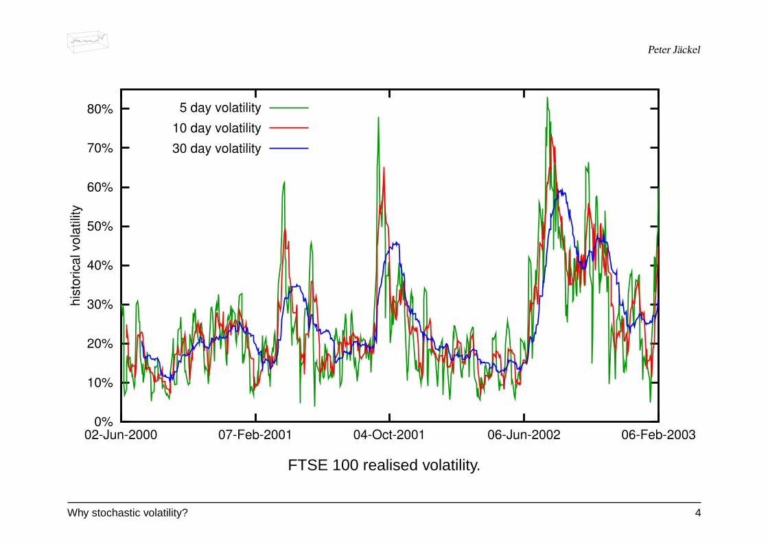
• Realised volatility of traded assets displays significant variability. It wouldonly seem natural that any model used for the hedging of derivative con-tracts on such assets should take into account that volatility is subject tofluctuations.

• More and more derivatives are explicitly sensitive to future (both impliedand instantaneous) volatility levels. Examples are cliquets, globally flooredand/or capped cliquets, and many more.

• Some (apparently) comparatively straightforward exotic derivatives suchas double barrier options are being being re-examined for their sensitivityto uncertainty in volatility.

• New trading ideas such as exotic volatility options and skew swaps, how-ever, give rise to the need for a new kind of stochastic volatility model: thestochastic skew model.

Why stochastic volatility? 2

Peter Jackel

3500

4000

4500

5000

5500

6000

6500

7000

02-Jun-2000 07-Feb-2001 04-Oct-2001 06-Jun-2002 06-Feb-2003

FTSE100

FTSE 100.


Peter Jackel

0%

10%

20%

30%

40%

50%

60%

70%

80%

02-Jun-2000 07-Feb-2001 04-Oct-2001 06-Jun-2002 06-Feb-2003

hist

oric

al v

olat

ility

5 day volatility

10 day volatility

30 day volatility

FTSE 100 realised volatility.


Peter Jackel

What stochastic volatility?

The concept of stochastic volatility, or rather the idea of a second sourceof risk affecting the level of instantaneous volatility, should not be seen inisolation from the nature of the underlying asset or deliverable contract.

For the three most developed modelling domains of equity, FX, and inter-est rate derivatives, different effects are considered to be at least partiallyresponsible for the smile or skew observed in the associated option markets.

What stochastic volatility? 5

Peter Jackel

Economic effects giving rise to an equity skew

• Leverage effects [Ges77, GJ84, Rub83]. A firm’s value of equity can beseen as the net present value of all its future income plus its assets minusits debt. These constituents have very different relative volatilities whichgives rise to a leverage related skew.

• Supply and demand. Equivalently, downwards risk insurance is more de-sired due to the intrinsic asymmetry of positions in equity: by their finan-cial purpose it is more natural for equity to be held long than short, whichmakes downwards protection more important.

• Declining stock prices are more likely to give rise to massive portfolio re-balancing (and thus volatility) than increasing stock prices. This asymme-try arises naturally from the existence of thresholds below which positionsmust be cut unconditionally for regulatory reasons.


Peter Jackel

Economic effects giving rise to an FX skew and smile

• Anticipated government intervention to stabilise FX rates.

• Government changes that are expected to change policy on trade deficits,interest rates, and other economic factors that would give rise to a marketbias.

• Foreign investor FX rate protection.

Economic effects giving rise to an interest rate skew and smile

• Elasticity of variance and/or mean reversion. In other words, interest ratesare for economic reasons linked to a certain band. Unlike equity or FX, in-terest rates cannot be split, bought back or re-valued and it is this intrinsicdifference that connects volatilities to absolute levels of interest rates.

• Anticipated central bank action.


Peter Jackel

None of these effects are well described by strong correlation be-tween the asset’s own driving factor and a second factor govern-ing the uncertainty in volatility since the are all based on deter-ministic relationships.

Still, most stochastic volatility models incorporate a skew byvirtue of strong correlation of volatility and stock. The strongcorrelation is usually needed to match the pronounced skew ofshort-dated plain vanilla options.

In this context, one might wonder if it wouldn’t be more ap-propriate to let the stochasticity of volatility explain the market-observed features related to or associated with uncertainty involatility, and use other mechanisms to account for the skew.


Peter Jackel

One model to rule them all?

An important question that must be asked when a stochastic volatility modelis considered is: what is it to be used for?

• Single underlying moderate exotics with strong dependence on forwardvolatility? Forward starting options? Cliquets?

• Single underlying exotics with strong dependence on forward skew? Glob-ally floored and/or capped cliquets and friends?

• Single underlying exotics with strong path dependence? Barriers of allnatures (single, double, layered, range accruals).

One model to rule them all? 9

Peter Jackel

• Multiple underlying moderate exotics with strong dependence on forwardvolatility? Options on baskets. Cliquets on baskets.

• Multiple underlying moderate exotics with strong dependence on forwardskew? Mountain range options.

• Multiple underlying moderate exotics with strong dependence on correla-tion? Mountain range options.

Not all of these applications would necessarily suggest the use of the samemodel!

A stochastic volatility model that can be perfectly adequate to capture the riskin one of the above categories may completely miss the exposures in otherproducts.

Example: consider the use of a conventional stochastic volatility model forthe management of options on variance swaps versus the use of the samemodel for options on future market skew in the plain vanilla option market.

One model to rule them all? 10

Peter Jackel

Mathematical features of stochastic volatility models

Heston [Hes93]: V[σ2

S

]∼ O

(σ2

S

)(mean reverting)

dS = µSdt +√

vS dWS (1)

dv = κ(θ − v)dt + α√

v dWv (2)

E[dWS · dWv] = ρ dt (3)

In order to achieve calibration to the market given skew, almost always:

• 0.7 < |%| . 1 is required.

• κ must be very small (kappa kills the skew).

• α must be sizeable.

• θ is by order of magnitude not too far away from the implied volatility of thelongest dated option calibrated to.

Mathematical features of stochastic volatility models 11

Peter Jackel

The volatility process can reach zero unless [Fel51, RW00]

κθ >12α2 (4)

which is hardly ever given in a set of parameters calibrated to market!

This means the Heston model achieves calibration to today’s observed plainvanilla option prices by balancing the probabilities of very high volatility sce-narios against those where future instantaneous volatility drops to very lowlevels.

The average time volatility stays at high or low levels is measured by themean reversion scale 1/κ.


Peter Jackel

Even when κθ > 12α

2, the long-term distribution of∫ t+τ

tσ(t)2dt is sharply

peaked at low values of volatility as a result of calibration1.

The dynamics of the calibrated Heston model predict that:

volatility can reach zero,

stay at zero for some time,

or stay extremely low or very high for long periods of time.

1see http://www.dbconvertibles.com/dbquant/Presentations/LondonDec2002RiskTrainingVolatility.pdf,slides 33–35, for diagrams on this feature.


http://www.dbconvertibles.com/dbquant/Presentations/LondonDec2002RiskTrainingVolatility.pdf

Peter Jackel

Stein and Stein / Schobl and Zhu [SS91, SZ99]: V[σS] ∼ O (1) (mean revert-ing)

dS = µSdt + σS dWS (5)

dσ = κ(θ − σ)dt + α dWσ (6)

E[dWS · dWσ] = ρ dt (7)

The distribution of volatility converges to a Gaussian distribution with mean θ

and variance α2

2κ . Since the sign of σ bears meaning only as a sign modifierof the correlation, we have the following two consequences:

• The sign of correlation between movements of the underlying and volatilitycan suddenly switch.

• The level of volatility has its most likely value at zero.


Peter Jackel

0

0.1

0.2

0.3

0.4

0.5

0.6

0.7

0.8

0% 20% 40% 60% 80% 100% 120%

ψ(σ

)

σ

ϕ(σ)ϕ(−σ)

ϕ(σ)+ϕ(−σ)

Stationary Stein & Stein volatility distribution for α = 0.3, κ = 0.3, and θ = 0.25.


Peter Jackel

The dynamics of the Stein and Stein / Sch obl and Zhu modelpredict that:

volatility is very likely to be near zero,

and that the sign of correlation with the spot movementdriver can switch.


Peter Jackel

Hull-White [HW87]: V[σ2

S

]∼ O

(σ4

S

)(zero reverting for µv < 0)

dS = µSS dt +√

vS dWS (8)

dv = µvv dt + ξv dWσ (9)


Since v is lognormally distributed in this model, and since σ =√

v, we have

E[σ(t)] = σ(0) · e12µvt−1

8ξ2t (11)

V[σ(t)] = σ(0)2 · eµvt ·(1− e−

14ξ2t

)(12)

M[σ(T )] = σ(0) · e12(µv−ξ2)t (13)

where M[·] is defined as the most likely value.

This means, for µv < 14ξ

2, the expectation of volatility converges to the mean-reversion level at zero. For µv > 1

4ξ2, the expectation diverges.


Peter Jackel

Further, unless µv < 0, the variance of volatility grows unbounded. In con-trast to that, if µv < 0, the variance of variance diminishes over time. Andfinally, the most likely value for volatility converges to zero unless µv > ξ2.

For the particular case of µv = 0, we have the special combination of featuresthat the expectation and most likely value of volatility converges to zero, whilstthe variance of volatility converges to σ2.

Any choice of parameters that provides a reasonable match of market givenimplied volatilities is extremely likely to lead to µv < 0 in which case we have:

The dynamics of the Hull-White stochastic volatility modelpredict that:

both expectation and most likely value of instantaneousvolatility converge to zero.


Peter Jackel

Hagan [HKL02]: V[σS] ∼ O(σ2

S

)(not mean reverting)

dS = µS dt + σS dWS (14)

dσ = ασ dWσ (15)


This model is equivalent to the Hull-White stochastic volatility model for thespecial case of µv = α2 and ξ = 2α. In this model, instantaneous volatilityis a martingale but the variance of volatility grows unbounded. At the sametime, the most likely value for volatility converges to zero.


Peter Jackel

The dynamics of the Hagan model predict that:

the expectation of volatility is constant over time,

that variance of instantaneous volatility grows without limit,

and that the most likely value of instantaneous volatilityconverges to zero.


Peter Jackel

Scott and Scott-Chesney [Sco87, CS89]: V[σS] ∼ O(σ2

S

)(mean reverting)

dS = µSdt + eyS dWS (17)

dy = κ (θ − y) dt + α dWy (18)

E[dWS · dWy] = ρ dt (19)

Volatility cannot reach zero, nor does its most likely value converge there.

3000

4000

5000

6000

7000

0 0.5 1 1.5 2 2.520%

30%

40%

50%

t [years]

S

σ

Sample path for Scott-Chesney model with S0 = 6216, r = 5%, d = 1%, σ0 = 30%, θ = ln 30%, κ = 0.1, α = 40%, α2

2κ = 2, ρ = 0. Euler integration with ∆t = 1/365.


Peter Jackel

The market-observable skew of implied volatilities would require a strongnegative correlation for this model to be calibrated.

2000

3000

4000

5000

6000

7000

0 0.5 1 1.5 2 2.510%

20%

30%

40%

50%

60%

70%

t [years]

S

σ

Sample path for Scott-Chesney model with S0 = 6216, r = 5%, d = 1%, σ0 = 30%, θ = ln 30%, κ = 0.1, α = 40%, α2

2κ = 2, ρ = −0.9. Euler integration with ∆t = 1/365.

However, the required strong correlation between volatility and spot is notsupported by any econometric analysis.


Peter Jackel

Nonetheless, it is possible to reproduce the burstiness of real volatility returnsby increasing the mean reversion.

2000

3000

4000

5000

6000

7000

8000

0 0.5 1 1.5 2 2.510%

20%

30%

40%

50%

60%

70%

80%

t [years]

S

σ

Sample path for Scott-Chesney model with S0 = 6216, r = 5%, d = 1%, σ0 = 30%, θ = ln 30%, κ = 6, α = 1.5, α2

2κ = 0.125, ρ = 0. Euler integration with ∆t = 1/2920.


Peter Jackel

Fouquet et alii compare strong mean reversion dynamics with real dataand find that it captures the apparent burstiness of realised volatilities verywell [FPS00]:

• The larger κ, the more rapidly the volatility distribution converges to itsstationary state.

• 1/κ is the time scale for volatility auto-decorrelation.

• The right measure for uncertainty in volatility is

α2

2κ,

not α on its own.

Large mean reversion causes volatility to approach its stationary distributionquickly.


Peter Jackel

The problem with future volatility being likely to hover near zero for modelssuch as the Heston and the Stein & Stein model goes away when meanreversion is strong.

However, if mean reversion is large, correlation between volatility and spotdoes not suffice to generate a significant skew.

To achieve market calibration, a different mechanism is needed. This couldbe independent jumps of the stock itself, or a stock-dependent volatility scal-ing function.


Peter Jackel

The main drawback of the Scott-Chesney model is that:

it requires very high correlation between the spot and thevolatility process to calibrate to a pronounced skew,

and that the skew is fully deterministic.

These features are also shared by all of the above discussedmodels.


Peter Jackel

A stochastic skew model

dS = µSdt + σf(S; γ)SdWS (20)

d lnσ = κσ(lnσ∞ − lnσ)dt + ασdWσ (21)

dγ = κγ(γ∞ − γ)dt + αγdWγ (22)

with

f(S; γ) = eγ·( SH−1) (23)

andE[dWσdWγ] = E[dWσdWS] = E[dWγdWS] = 0 (24)

A stochastic skew model 27

Peter Jackel

This scaling ensures that:-

• For negative γ, the local volatility scaling factor decays from e−γ for S → 0to 0 for S →∞.

• The local volatility scaling factor f at spot level H is exactly 1.

• The local volatility scaling factor f change for a spot move of δ ·H near His given by

∆f =∂f

∂S

∣∣∣∣S=H

· δ ·H =γ

H· δ ·H = δ · γ . (25)

In other words, γ is a measure for the local volatility skew at H.


Peter Jackel

Maintenance of correlation matrices is greatly simplified by the assumptionof independence of the individual factors.

The associated partial differential equation governing the boundary valueproblem of derivatives prices is

Vt +(µ− 1

2e2yf2(ex; γ))︸︷︷︸

µx

Vx + κσ (lnσ∞ − y)︸︷︷︸µy

Vy + κγ (γ∞ − γ)︸︷︷︸µγ

Vγ (26)

+12e2yf2(ex; γ)Vxx + 1

2α2σVyy + 1

2α2γVγγ = r · V

withx = ln S and y = ln σ . (27)


Peter Jackel

0.08

0.42

0.75

1.08

1.42

1.75

2.08

2.420.5 0.6 0.7 0.8 0.9 1 1.1 1.2 1.3 1.4 1.5 1.6 1.7 1.8 1.9 2

25%

30%

35%

40%

45%

50%

55%

implied volatility

T

K/S

Implied volatility surface for stochastic skew model with S0 = H = 6216, r = 5%, d = 1%,

σ0 = σ∞ = 30%, κσ = 12, ασ = 2,

√α2

σ2κσ

= 41%, γ0 = γ∞ = −0.5, κγ = 4, αγ = 0.5,

√α2

γ2κγ

= 0.18.


Peter Jackel

Jumps without jumps

The exponential dependence of the volatility scaling function f on the spotlevel S can lead to jump-like upward (for γ > 0) or dowward (for γ < 0) rallieswhen |γ| is of significant size.

0

1000

2000

3000

4000

5000

6000

0 0.5 1 1.5 2 2.5

t [years]

S

Jump-like almost instantaneous downwards corrections of the spot for S0 = H = 6216, r = 5%, d = 1%,

σ0 = σ∞ = 25%, κσ = 6, ασ = 1,

√α2

σ2κσ

= 29%, γ0 = γ∞ = −2, κγ = 3, αγ = 2,

√α2

γ2κγ

= 0.82.


Peter Jackel

This can happen due to the exponential nature of the scaling function f , especially duringperiods of increased |γ|.

10%

15%

20%

25%

30%

35%

40%

45%

0 0.5 1 1.5 2 2.5

σ

-4

-3.5

-3

-2.5

-2

-1.5

-1

-0.5

0 0.5 1 1.5 2 2.5

t [years]

γ


Peter Jackel

These events only occur when the skew is very pronounced:

0.08

0.33

0.58

0.83

1.08

1.33

1.58

1.83

2.08

2.33

2.58

0.5 0.6 0.7 0.8 0.9 1 1.1 1.2 1.3 1.4 1.5 1.6 1.7 1.8 1.9 2

14%

19%

24%

29%

34%

39%

44%

49%

54%

implied volatility

T

K/S

Implied volatility surface for stochastic skew model with S0 = H = 6216, r = 5%, d = 1%,

σ0 = σ∞ = 25%, κσ = 6, ασ = 1,

√α2

σ2κσ

= 29%, γ0 = γ∞ = −2, κγ = 3, αγ = 2,

√α2

γ2κγ

= 0.82.


Peter Jackel

A hyperbolic alternative

The shown implosions of the spot are caused by the exponential form of the scaling functionf and are technically akin to process explosions seen also for the short rate in a lognormalHJM setting and other equations involving a locally exponential scaling of volatility. Naturally,it is straightforward to use other scaling functions that avoid the spot implosions, should theybe undesirable.

An alternative to the exponential scaling is the hyperbolic function

f = γ

(S

H− 1

)+

√γ2

(S

H− 1

)2

+ (1− η)2 + η (28)

0

0.5

1

1.5

2

2.5

0 50 100 150 200 250

hyperbolic form for f(S)

Hyperbolic example for the scaling function f(S) with γ = −1, H = 100, and η = 1/4.


Peter Jackel

0.08

0.42

0.75

1.08

1.42

1.75

2.08

2.420.5 0.6 0.7 0.8 0.9 1 1.1 1.2 1.3 1.4 1.5 1.6 1.7 1.8 1.9 2

15%

20%

25%

30%

35%

40%

45%

50%

implied volatility

T

K/S

Implied volatility surface for stochastic skew model with a hyperbolic scaling function f and S0 = H = 6216, r = 5%, d = 1%,

σ0 = σ∞ = 25%, κσ = 6, ασ = 1,

√α2

σ2κσ

= 28.87%, γ0 = γ∞ = −3, κγ = 3, αγ = 3,

√α2

γ2κγ

= 1.22, and η = 1/4.


Peter Jackel

Monte Carlo methods and stochastic volatility models

The Heston model is often used to parametrise the observed market volatil-ities since there are semi-analytical solutions for plain vanilla options underthis model.

However, when multi-asset derivatives are priced, we often need to resort tonumerical integration of the governing stochastic differential equations.

Euler discretisation of the Heston variance process:

∆v = κ(θ − v)∆t + α√

v√

∆t · z (29)

with z ∼ N (0, 1). This means for z < z∗ with

z∗ = −v + κ(θ − v)∆t

α√

v∆t(30)

the Euler step causes variance to cross over to the negative domain!

Monte Carlo methods and stochastic volatility models 36

Peter Jackel

A popular method of choice to avoid this artifact of Euler integration is to useIto’s lemma to transform to coordinates where the Euler step remains in thedomain of validity for all possibly drawn Gaussian variates. For the Hestonvariance process, the coordinate we have to transform to is volatility itself:

dσ =κ2

[1σ

(θ − α2

4κ

)− σ

]dt + 1

2α dW (31)

Alas, it seems we have transformed ourselves from the pan into the fire: whilst equation (2)would always show a positive drift term for all θ > 0 no matter how close variance came tozero, and only the diffusion component could make it reach zero, the drift term in equation(31) diverges to negative infinity if θ < α2

4κ irrespective of the path taken by the diffusioncomponent.

This means, the transformed equation shows strong (drift-dominated) absorption into zeronear zero, whilst the original stochastic differential equation for the variance only exhibitszero as an attainable boundary due to the diffusion component being able to overcome themean reversion effect (i.e. the positive drift) for 2θκ < α2.


Peter Jackel

The apparently contradictory behaviour near zero has a simple explanation:

In an infinitesimal neighbourhood of zero, It o’s lemma cannot beapplied to the variance process ( 2).

The transformation of the variance process to a volatilityformulation results in a structurally different process !

Naturally, this feature raises its ugly head in any numerical implementationwhere we may prefer to use a transformed version of the original equations!

An alternative, when suitable transformations are not available, is to use im-plicit or mixed Euler schemes [KP99] in order to ensure that the steppingalgorithm does not cause the state variable to leave the domain of the gov-erning equations, possibly in conjunction with Doss’s [Dos77] method of con-structing pathwise solutions.


Peter Jackel

An example for such an approach is as follows.

First, let us assume that we have discretised the evolution of time into asequence of time intervals [tn, tn+1], and that we have drawn an independentWiener path over those points in time, i.e. that we know W (tn) for all n forone specific path.

Then, approximate W (t) as a piecewise linear function in between the knownvalues at tn and tn+1, i.e.

W (t) ' γn + δnt for t ∈ [tn, tn+1] (32)

with

γn = W (tn)− δntn and δn =W (tn)−W (tn+1)

tn − tn+1.

Using the resulting dependency dW = δndt, this gives us the approximateordinary differential equation

dv

dt' κ(θ − v) + αδn

√v (33)


Peter Jackel

which has the implicit solution

t− tn = T (v(t))− T (v(tn)) (34)

with

T (v) =2αδn

κ√

α2δ2n + 4θκ2

atanh

(2κ√

v − αδn√α2δ2

n + 4θκ2

)−

1

κln(κ (v − θ)− αδn

√v)

(35)

The above equation can be solved numerically comparitively readily since weknow that, given δn, over the time step from tn to tn+1, v will move monoton-ically, and that in the limit of ∆tn := (tn+1 − tn) → ∞, for fixed δn, we have

lim∆tn→∞

vn+1 =

αδ

2κ+

√(αδ

2κ

)2

+ θ

2

(36)

which can be computed by setting the argument of the logarithm in the righthand side of equation (35) to zero.


Peter Jackel

0%

10%

20%

30%

40%

50%

60%

70%

0 0.2 0.4 0.6 0.8 1

σ(t)

t

δ = 5δ = 4δ = 3δ = 2δ = 1δ = 0δ = -1δ = -2δ = -3δ = -4δ = -5

Sample paths for the Heston volatility process for σ(0) =√

v(0) = 20%,√

θ = 15%, α = 30%, κ = 1 over a unit time step for different levels of the variateδ = Wv(1)−Wv(0) when Wv(t) is approximated linearly over the time step.

Putting all of the above together enables us to construct paths for thestochastic variance without the need for very small time steps.


Peter Jackel

The explicit knowledge of the functional form of the volatility, or variance, pathhas another advantage:

Fouquet et alii [FPS00] explain how we can directly draw the logarithm ofthe spot level at the end of a large time step (tn+1 − tn) if we can explicitlycompute, for the given volatility or variance path, the quantities

∆vn :=

tn+1∫tn

σ2(t) dt (37)

∆ωn :=

tn+1∫tn

σ(t) dW (t) (38)


Peter Jackel

The first term poses no difficulty since the primitive of T (v) can be computedanalytically and

tn+1∫tn

σ2(t) dt = v(tn+1) · [T (v(tn)) + ∆tn] − v(tn) · T (v(tn)) −vn+1∫vn

T (v) dv .

(39)The second term requires another approximate numerical scheme which willalso be no major obstacle since

tn+1∫tn

σ(t) dW (t) ' δn ·tn+1∫tn

σ(t) dt

= δn ·(σ(tn+1) · [T (v(tn)) + ∆tn] − σ(tn) · T (v(tn))

−vn+1∫vn

T (v)/ (2√

v) dv)

. (40)


Peter Jackel

The numerical approximation is needed for the calculation of the integral onthe right hand side of equation (40).

A simple Simpson scheme or Legendre quadrature will produce excellentresults given that the function is guaranteed to be monotonic and smooth.

Using all of the above quantities, the draw for the logarithm of the spot levelcan be constructed as

lnSn+1 = ln Sn + µ∆tn −12∆vn + ρ∆ωn +

√1− ρ2 ·

√∆vn · z (41)

where z is a standard normal variate that is independent from the variateused to construct the variance step vn → vn+1.


Peter Jackel

The above scheme is essentially an extension of the root-mean-squarevolatility lemma given in [HW87] beyond the case of ρ = 0.

In comparison, the Stein and Stein / Schobl and Zhu, Hull-White, Haganand Scott/Scott-Chesney model can be simulated much more easily sincethe stochastic differential equation for the volatility component has simpleanalytical solutions.

Naturally, similar techniques to the one elaborated above for the Hestonmodel can be used to obviate the need for very small time steps.


Peter Jackel

Finite differencing methods and stochastic volatility models

Non-zero correlation between the different factors makes it impossible to useAlternating Direction Implicit methods (unless we transform away the corre-lation term which is usually very bad for the handling of boundary conditions,or we combine it with an explicit method for the cross terms which makes thescheme effectively explicit). Explicit methods require rather small time stepsin order to avoid explosions due to numerical instabilities.

The multi-dimensional equivalent of the Crank-Nicolson method (also de-noted as Peaceman-Rachford-Douglas method [PR55, DR56]) can be im-plemented efficiently using iterative solver algorithms such as the stabilisedbiconjugate gradient method [GL96] that don’t require the explicit specifica-tion of the matrix at all.

All that is needed is a function that carries out the same calculations thatwould be done in an explicit method. A useful collection of utilities for thispurpose is the Iterative Template Library [LLS].

Finite differencing methods and stochastic volatility models 46

Peter Jackel

For the stochastic skew model, the independence of the three factors makesit possible to use a three factor Alternating Direction Implicit version of theCrank Nicolson method. This means it is possible to have large time steps ina fast finite differencing scheme.

Since we have zero correlation in the stochastic skew model, the numberof discretisation layers in both the volatility and the skew factor can be keptsmall (∼ 20–30).

Also, boundary conditions can be kept simple in all directions and in thecorners: Vii = 0 for i = x, y, γ.

The speed of three factor ADI implementations is compatible with that of anysafe implementation involving numerical contour integrals or Fourier inver-sions of characteristic functions etc.


Peter Jackel

The generalisation of Alternating Direction Implicit (or Alternating DirectionCrank-Nicolson) to multiple spatial dimensions is based on the idea of anoperator split [PR55, DR56, Mar89].

Take the equation

Vt +∑

i

µi(t, x)Vxi+ 1

2

∑i

σ2i (t, x)Vxixi

= r · V, (42)

transform away the source term by setting u := V e−rt (which almost certainly changes yourboundary conditions)

ut +∑

i

(µi∂xi

+ 12σ

2i ∂

2xi

)︸︷︷︸

Li

·u = 0 . (43)

i.e.(∂t + L) · u = 0 with L =

∑i

Li . (44)


Peter Jackel

Finite differencing of accuracy order O(∆t2):

∂t · u →1

∆t[u(t, x)− u(t−∆t, x)] (45)

∂xi · u →1

2∆xi

[u(t, . . . , xi + ∆xi, . . .)− u(t, . . . , xi −∆xi, . . .)

](46)

∂2xi· u →

1

∆x2i

[u(t, . . . , xi + ∆xi, . . .)− 2u(t, . . . , xi, . . .) + u(t, . . . , xi −∆xi, . . .)

](47)

Discretisation of the differential operators yields Li → Di with

Di · u(t, x) = µi(t, x)1

2∆xi

[u(t, . . . , xi + ∆xi, . . .)− u(t, . . . , xi −∆xi, . . .)

](48)

+1

2σ

2i (t, x)

1

∆x2i

[u(t, . . . , xi + ∆xi, . . .)− 2u(t, x) + u(t, . . . , xi −∆xi, . . .)

]

Di · u(x) =1

2∆x2i

[ (σ

2i (t, x) + µi(t, x)∆xi

)u(. . . , xi + ∆xi, . . .) − 2σ

2i (t, x)u(x)

+(

σ2i (t, x)− µi(t, x)∆xi

)u(. . . , xi + ∆xi, . . .)

](49)


Peter Jackel

Crank-Nicolson:

(∂t + L) · u(t, x) = 0 (50)

is to be approximated by

1

∆t

[u(t, x)− u(t−∆t, x)

]+ 1

2D ·[u(t, x) + u(t−∆t, x)

]= 0 (51)

This means, a single step in the Crank-Nicolson scheme is given by solving(1− 1

2∆tD)· u(t−∆t, x) =

(1 + 1

2∆tD)· u(t, x) (52)

for u(t−∆t, x).

The operator split of the discretised operator D =∑

i Di is to split D into itscommuting components {Di}, and to solve (52) for each of the Di individuallyin sequence.


Peter Jackel

A single time step in the n-dimensional operator-split finite differencingscheme is thus given by a sequence of n one-dimensional finite differenc-ing steps. Solve:(

1− 12∆tD1

)· u(1)(x) =

(1 + 1

2∆tD1

)· u(t, x)(

1− 12∆tD2

)· u(2)(x) =

(1 + 1

2∆tD2

)· u(1)(x)

... ... ...(1− 1

2∆tDn

)· u(n)(x) =

(1 + 1

2∆tDn

)· u(n−1)(x)

and set

u(t−∆t, x) := u(n)(x) .


Peter Jackel

For commuting Di and Dj, i.e. DiDj = DjDi, this scheme is, like the one-dimensional Crank-Nicolson method, of convergence order O

(∆t2

):

u(j)(x) =(1− 1

2∆tDi

)−1 ·(1 + 1

2∆tDi

)· u(j−1)(x)

=(1 + 1

2∆tDi + 14∆t2D2

i

)·(1 + 1

2∆tDi

)· u(j−1)(x) +O

(∆t3

)=

(1 + ∆tDi + 1

2∆t2D2i

)· u(j−1)(x) +O

(∆t3

)(53)

=⇒

u(t−∆t) =

[∏i

(1 + ∆tDi + 1

2∆t2D2i

)]· u(t) +O

(∆t3

)

=

1 + ∆t∑

i

Di + 12∆t2

∑i,j

DiDj

· u(t) +O(∆t3

)(54)


Peter Jackel

Equation (54) is of precisely the same form as the one we obtain for u in tfrom the continuous equation (∂t + L) · u = 0 :

u(t−∆t) =

1 + ∆t∑

i

Li + 12∆t2

∑i,j

LiLj

· u(t) +O(∆t3

)(55)

In order to avoid a building up of lower order error terms due to the fact thatDi and Dj don’t always commute perfectly (primarily due to the boundaryconditions, but also due to round-off), the ordering of the scheme can bepermuted.

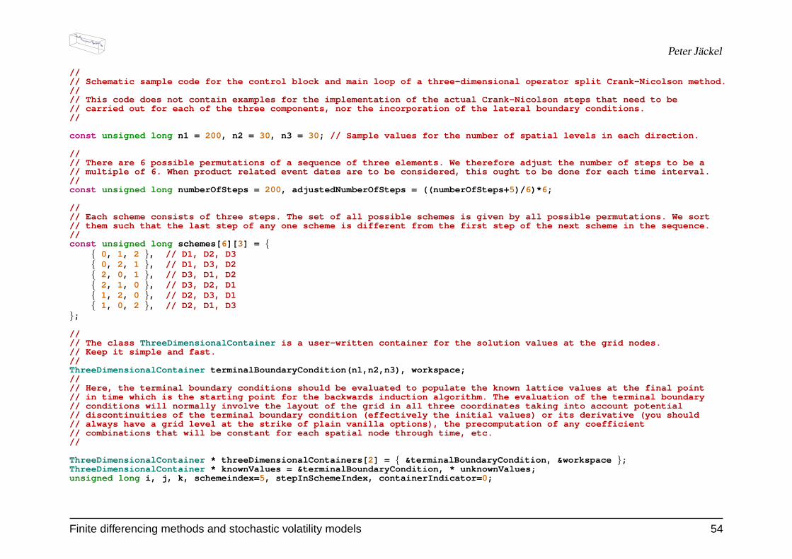
For a three-factor model, this means there are 3! = 6 permutations that wecan cycle through as shown in the following example.


Peter Jackel

//// Schematic sample code for the control block and main loop of a three-dimensional operator split Crank-Nicolson method.//// This code does not contain examples for the implementation of the actual Crank-Nicolson steps that need to be// carried out for each of the three components, nor the incorporation of the lateral boundary conditions.//

const unsigned long n1 = 200 , n2 = 30, n3 = 30; // Sample values for the number of spatial levels in each direction.

//// There are 6 possible permutations of a sequence of three elements. We therefore adjust the number of steps to be a// multiple of 6. When product related event dates are to be considered, this ought to be done for each time interval.//const unsigned long numberOfSteps = 200 , adjustedNumberOfSteps = ((numberOfSteps+ 5)/ 6)* 6;

//// Each scheme consists of three steps. The set of all possible schemes is given by all possible permutations. We sort// them such that the last step of any one scheme is different from the first step of the next scheme in the sequence.//const unsigned long schemes[ 6][ 3] = {

{ 0, 1, 2 }, // D1, D2, D3{ 0, 2, 1 }, // D1, D3, D2{ 2, 0, 1 }, // D3, D1, D2{ 2, 1, 0 }, // D3, D2, D1{ 1, 2, 0 }, // D2, D3, D1{ 1, 0, 2 }, // D2, D1, D3

};

//// The class ThreeDimensionalContainer is a user-written container for the solution values at the grid nodes.// Keep it simple and fast.//ThreeDimensionalContainer terminalBoundaryCondition(n1,n2,n3), workspace;//// Here, the terminal boundary conditions should be evaluated to populate the known lattice values at the final point// in time which is the starting point for the backwards induction algorithm. The evaluation of the terminal boundary// conditions will normally involve the layout of the grid in all three coordinates taking into account potential// discontinuities of the terminal boundary condition (effectively the initial values) or its derivative (you should// always have a grid level at the strike of plain vanilla options), the precomputation of any coefficient// combinations that will be constant for each spatial node through time, etc.//

ThreeDimensionalContainer * threeDimensionalContainers[ 2] = { &terminalBoundaryCondition, &workspace };ThreeDimensionalContainer * knownValues = &terminalBoundaryCondition, * unknownValues;unsigned long i, j, k, schemeindex= 5, stepInSchemeIndex, containerIndicator= 0;


Peter Jackel

//// The main loop of backward induction.//for (i=0;i<adjustedNumberOfSteps;++i) {

++schemeindex %= 6;for (stepInSchemeIndex= 0;stepInSchemeIndex< 3;++stepInSchemeIndex) {

++containerIndicator %= 2;unknownValues = threeDimensionalContainers[containerIndicator];switch (schemes[schemeindex][stepInSchemeIndex]) {

case 0 : //// Crank-Nicolson step in D1 to be placed here.//

break ;case 1 : //

// Crank-Nicolson step in D2 to be placed here.//

break ;case 2 : //

// Crank-Nicolson step in D3 to be placed here.//

break ;}knownValues = threeDimensionalContainers[containerIndicator];

}}

//// Assuming that the grid levels are stored in the three one-dimensional vectors x1Values[], x2Values[], and// x3Values[], and that the spot coordinates are given by x1, x2, and x3, and that we have already asserted that// (x1,x2,x3) is inside the grid, we interpolate the solution at (x1,x2,x3) from the grid values.//for (i= 0;x1Values[i]<x1;++i); for (j= 0;x2Values[j]<x2;++j); for (k= 0;x3Values[k]<x3;++k);

const double p1 = (x1-x1Values[i- 1])/(x1Values[i]-x1Values[i- 1]), q1 = 1 - p1;const double p2 = (x2-x2Values[j- 1])/(x2Values[j]-x2Values[j- 1]), q2 = 1 - p2;const double p3 = (x3-x3Values[k- 1])/(x3Values[k]-x3Values[k- 1]), q3 = 1 - p3;

//// Below, we assume that an object v of class ThreeDimensionalContainer allows you to retrieve// the value at the (i,j,k) grid coordinates by the use of the notation v(i,j,k).//const ThreeDimensionalContainer &v = *knownValues;//// Trilinear interpolation.//const double solution = p1*p2*p3*v(i,j,k) + p2*q1*p3*v(i- 1,j,k) + p1*q2*p3*v(i,j- 1,k) + q1*q2*p3*v(i- 1,j- 1,k)

+ p1*p2*q3*v(i,j,k- 1) + p2*q1*q3*v(i- 1,j,k- 1) + p1*q2*q3*v(i,j- 1,k- 1) + q1*q2*q3*v(i- 1,j- 1,k- 1);


Peter Jackel

References[Baa97] B. E. Baaquie. A Path Integral Approach to Option Pricing with Stochastic Volatility : Some Exact Results. Journal de Physique, 1(7):1733–1753, 1997.[CN47] J. Crank and P. Nicolson. A practical method for numerical evaluation of solutions of partial differential equations of the heat-conduction type. Proc. Camb. Philos.

Soc., 43:50–67, 1947.[CS89] M. Chesney and L. Scott. Pricing European Currency Options: A comparison of the modified Black-Scholes model and a random variance model. Journal of

Financial and Quantitative Analysis, 24:267–284, September 1989.[Dos77] H. Doss. Liens entre equations differentielles stochastiques ordinaires. Annales de l’Institut Henrie Poincare. Probabilites et Statistiques, 13:99–125, 1977.[DR56] J. Douglas and H. H. Rachford. On the numerical solution of heat conduction problems in two and three space variables. Transactions of the American Mathematical

Society, 82:421–439, 1956.[Fel51] W. Feller. Two Singular Diffusion Problems. Annals of Mathematics, 54:173–182, 1951.[FPS00] J.-P. Fouque, G. Papanicolaou, and K. R. Sircar. Derivatives in Financial Markets with Stochastic Volatility. Cambridge University Press, September 2000. ISBN

0521791634.[Ges77] R. Geske. The Valuation of Corporate Liabilities as Compound Options. Journal of Financial and Quantitative Analysis, 12:541–552, 1977.[GJ84] R. Geske and H. E. Johnson. The Valuation of Corporate Liabilities as Compound Options: A Correction. Journal of Financial and Quantitative Analysis, 19:231–232,

1984.[GL96] G. H. Golub and C. F. Van Loan. Matrix Computations. The John Hopkins University Press, 1983,1989,1996.[Hes93] S. L. Heston. A closed-form solution for options with stochastic volatility with applications to bond and currency options. The Review of Financial Studies, 6:327–343,

1993.[HKL02] P. Hagan, D. Kumar, and A. S. Lesniewski. Managing smile risk. Wilmott, pages 84–108, September 2002.[HW87] J. Hull and A. White. The Pricing of Options on Assets with Stochastic Volatilities. The Journal of Finance, 42(2):281–300, June 1987. fac-

ulty.baruch.cuny.edu/lwu/890/HullWhite87.pdf.[HW88] J. Hull and A. White. An Analysis of the Bias in Option Pricing Caused by a Stochastic Volatility. Advances in Futures and Options Research, 3:27–61, 1988.[Jac02] P. Jackel. Monte Carlo methods in finance. John Wiley and Sons, February 2002.[KP99] P. E. Kloeden and E. Platen. Numerical Solution of Stochastic Differential Equations. Springer Verlag, 1992, 1995, 1999.[LLS] A. Lumsdaine, L. Lee, and J. Siek. The iterative template library. www.osl.iu.edu/research/itl.[Mar89] G. I. Marchuk. Splitting and alternating direction methods. In J. Lions and P. Ciarlet, editors, Handbook of Numerical Analysis, Volume I, volume I, pages 197–462.

Elsevier Science Publishers, 1989.[Mer73] R. C. Merton. Theory of Rational Option Pricing. Bell Journal of Economics and Management Science, 4:141–183, Spring 1973.[Mer76] R. C. Merton. Option Pricing When Underlying Stock Returns are Discontinuous. Journal of Financial Economics, 3:125–144, 1976.[Mer90] R. C. Merton. Continuous-Time Finance. Blackwell Publishers Ltd., 1990.[MM94] K. W. Morton and D. F. Mayers. Numerical Solution of Partial Differential Equations. Cambridge University Press, 1994. ISBN 0521429226.[PR55] D. W. Peaceman and H. H. Rachford. The numerical solution of parabolic and elliptic differential equations. Journal of the Society for Industrial and Applied

Mathematics, 3:28–41, 1955.[PTVF92] W. H. Press, S. A. Teukolsky, W. T. Vetterling, and B. P. Flannery. Numerical Recipes in C. Cambridge University Press, 1992.[Rub83] M. Rubinstein. Displaced diffusion option pricing. Journal of Finance, 38:213–217, March 1983.[RW00] L. C. G. Rogers and D. Williams. Diffusions, Markov Processes and Martingales: Volume 2, Ito Calculus. Cambridge University Press, September 2000.

References 56

http://faculty.baruch.cuny.edu/lwu/890/HullWhite87.pdf

http://faculty.baruch.cuny.edu/lwu/890/HullWhite87.pdf

http://www.osl.iu.edu/research/itl

Peter Jackel

[Sco87] L. Scott. Option Pricing When the Variance Changes Randomly: Theory, Estimation and An Application. Journal of Financial and Quantitative Analysis, 22:419–438,December 1987.

[SS91] E. M. Stein and J. C. Stein. Stock Price Distribution with Stochastic Volatility : An Analytic Approach. Review of Financial Studies, 4:727–752, 1991.[SZ99] R. Schobel and J. Zhu. Stochastic Volatility With an Ornstein Uhlenbeck Process: An Extension. European Finance Review, 3:23–46, 1999.[TR00] D. Tavella and C. Randall. Pricing Financial Instruments: The Finite Difference Method. John Wiley and Sons, April 2000. ISBN 0471197602.[Wil00] P. Wilmott. Quantitative Finance. John Wiley and Sons, 2000.

References 57

Stochastic Volatility Models: Past, Present and Future

Documents

Transcript of Stochastic Volatility Models: Past, Present and Future