Stochastic Volatility - DiVA Portal
35
Stochastic Volatility Kristina Andersson U.U.D.M. Project Report 2003:18 Examensarbete i matematik, 20 poäng Handledare: Ola Hammarlid , Swedbank Markets Examinator: Johan Tysk November 2003 Department of Mathematics Uppsala University
Transcript of Stochastic Volatility - DiVA Portal

Stochastic Volatility
Kristina Andersson
U.U.D.M. Project Report 2003:18
Examensarbete i matematik, 20 poäng
Handledare: Ola Hammarlid , Swedbank Markets
Examinator: Johan Tysk
November 2003
Department of Mathematics
Uppsala University

Abstract
In the original Black-Scholes model, the risk is quantified by a con-stant volatility parameter. It has been proposed by many authors thatthe volatilities should be modeled by a stochastic process to obtain amore realistic model. The volatility that corresponds to actual mar-ket data for option prices in Black-Scholes model is called the impliedvolatility. This volatility is in general dependent on the strike price, incontrast to the underlying assumption of Black-Scholes model. As afunction of strike it forms a curve called ”volatility smile”. To explainthis smile it has been proposed to study models allowing for a volatil-ity driven by a stochastic process. In the present paper a review ofstochastic volatility is presented and three stochastic volatility modelsare studied in some detail. We study the volatility smile of these mod-els and show that in some cases we can reproduce a smile similar tothe curves occuring in reality. We also study a corrected Black-Scholespricing formula.

Contents
1 Introduction 3
2 Stochastic volatility 3
2.1 General pricing . . . . . . . . . . . . . . . . . . . . . . . . . . 42.2 Stochastic volatility models . . . . . . . . . . . . . . . . . . . 7
2.2.1 Hull-White . . . . . . . . . . . . . . . . . . . . . . . . 72.2.2 Cox-Ingersoll-Ross . . . . . . . . . . . . . . . . . . . . 82.2.3 Log Ornstein-Uhlenbeck . . . . . . . . . . . . . . . . . 8
3 The corrected pricing formula 10
3.1 Invariant distribution and important parameters . . . . . . . 113.2 The pricing partial differential equation in terms of ε . . . . . 113.3 Asymptotic solution . . . . . . . . . . . . . . . . . . . . . . . 123.4 Expression for V2 and V3 . . . . . . . . . . . . . . . . . . . . 15
3.4.1 Log Ornstein-Uhlenbeck . . . . . . . . . . . . . . . . . 163.4.2 Cox-Ingersoll-Ross . . . . . . . . . . . . . . . . . . . . 16
3.5 Implied volatility for a European call option . . . . . . . . . . 17
4 Simulation and estimation 18
4.1 Examples from the Swedish option market . . . . . . . . . . . 194.2 Hull-White model . . . . . . . . . . . . . . . . . . . . . . . . . 194.3 Methods for the continuous models . . . . . . . . . . . . . . . 224.4 Cox-Ingersoll-Ross model . . . . . . . . . . . . . . . . . . . . 244.5 Log Ornstein-Uhlenbeck model . . . . . . . . . . . . . . . . . 254.6 Estimated V2 and V3 . . . . . . . . . . . . . . . . . . . . . . . 26
5 Summary and discussion 30
6 Acknowledgements 30
A Appendix 31
A.1 Basic arbitrage theory . . . . . . . . . . . . . . . . . . . . . . 31
2

1 Introduction
A financial derivative, for example an option, is a contract defined in termsof some underlying asset which already exists on the market, such as astock. The simplest financial derivative is a European call option. A calloption gives the holder of the option the right, but not the obligation, tobuy the underlying asset to a given price, the strike price, at a given time,the expiration day. European options can thus only be exercised on theexpiration day. A European option can be priced by the Black-Scholesformula, see [1].
In the original Black-Scholes model, the risk is quantified by a constantvolatility parameter. A natural generalization is to model the volatility bya stochastic process. In reality, the volatility process cannot be directlyobserved. However, through empirical studies of the stock price returnsone has observed that the estimated volatility fluctuates randomly arounda mean level. The process is said to be mean-reverting.
The implied volatility I is defined to be the value of the volatility pa-rameter that must go into the Black-Scholes formula (121) in the Appendixto match the observed price, Cobs,
CBS(t, S,K, T, I) = Cobs , (1)
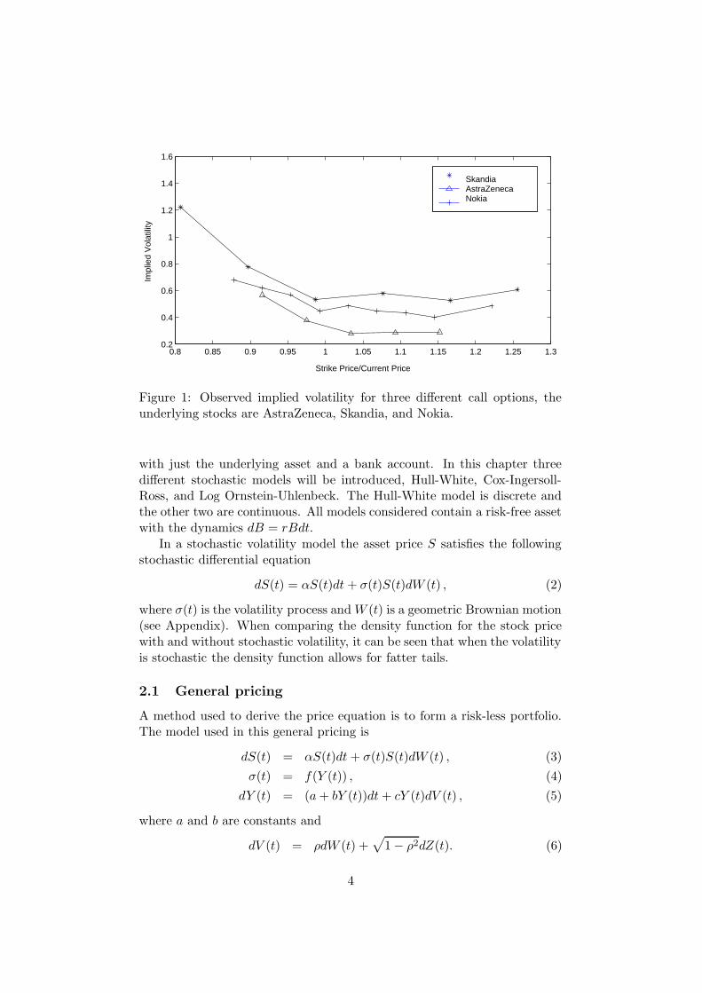
where CBS is the Black-Scholes price. When studying a real market pricethe implied volatility is not constant as assumed in Black-Scholes model,but varies. The result when plotting the implied volatility against K orthe ratio of the strike price to the current price is called the smile curveor volatility smile. It is interesting to investigate if there are any smileeffects in reality. In Figure 1 an example from the Swedish option marketis shown. The implied volatility is plotted against the ratio of the strikeprice to the current price for three different underlying stocks, AstraZeneca,Skandia, and Nokia. As seen in the figure there is a distinct smile effect forall options.
2 Stochastic volatility
In a stochastic volatility model the volatility is changing randomly accordingto some stochastic differential equation or some discrete random processes.Our main reference for this theory is [2]. A stochastic volatility modelintroduces more random sources then traded assets. According to generalmarket theory, see for instance the meta-theorem in [1], the model is notcomplete since the number of random sources is greater than the number ofunderlying traded assets. Pricing in a market with stochastic volatility isthus an incomplete market problem, which means that there does not exista unique martingale measure, and the derivative cannot be perfectly hedged
3
0.8 0.85 0.9 0.95 1 1.05 1.1 1.15 1.2 1.25 1.30.2
0.4
0.6
0.8
1
1.2
1.4
1.6
Strike Price/Current Price
Impl
ied
Vol
atili
ty
SkandiaAstraZenecaNokia
Figure 1: Observed implied volatility for three different call options, theunderlying stocks are AstraZeneca, Skandia, and Nokia.
with just the underlying asset and a bank account. In this chapter threedifferent stochastic models will be introduced, Hull-White, Cox-Ingersoll-Ross, and Log Ornstein-Uhlenbeck. The Hull-White model is discrete andthe other two are continuous. All models considered contain a risk-free assetwith the dynamics dB = rBdt.
In a stochastic volatility model the asset price S satisfies the followingstochastic differential equation
dS(t) = αS(t)dt + σ(t)S(t)dW (t) , (2)
where σ(t) is the volatility process andW (t) is a geometric Brownian motion(see Appendix). When comparing the density function for the stock pricewith and without stochastic volatility, it can be seen that when the volatilityis stochastic the density function allows for fatter tails.
2.1 General pricing
A method used to derive the price equation is to form a risk-less portfolio.The model used in this general pricing is
dS(t) = αS(t)dt+ σ(t)S(t)dW (t) , (3)
σ(t) = f(Y (t)) , (4)
dY (t) = (a+ bY (t))dt+ cY (t)dV (t) , (5)
where a and b are constants and
dV (t) = ρdW (t) +√
1 − ρ2dZ(t). (6)
4

The processes W and Z are uncorrelated but V and W are correlated.In the model described by equations (3)-(6) there is one traded asset S
and two random sources W (t) and Z(t). In this case there is two sourcesof randomness instead of one as in the standard Black-Scholes case. Whenconstructing a portfolio the derivatives cannot be perfectly hedged with justthe underlying asset. Instead we also need a benchmark derivative called G.A risk-less portfolio Π is formed, contain the quantity −∆S of the underlyingasset S, the quantity −∆G of another traded asset G (Benchmark option)and the priced derivative P . The total value of the portfolio is
Π = P − ∆SS − ∆GG . (7)
The differential of the portfolio value is needed to construct a risk-less andarbitrage free portfolio, equation (7) gives
dΠ = dP − ∆SdS − ∆GdG , (8)
can, by using Ito´s formula be written as
dΠ =
[
∂P
∂t+
1
2
∂2P
∂S2f(y)2S2 +
1
2
∂2P
∂y2c2 +
∂2P
∂S∂yf(y)Scρ
]
dt
+∂P
∂sdS +
∂P
∂ydY − ∆SdS
− ∆G
{
[
∂G
∂t+
1
2
∂2G
∂s2f(y)2S2 +
1
2
∂2G
∂y2c2 +
∂2G
∂S∂yf(y)Scρ
]
dt
+∂G
∂sdS +
∂G
∂ydY
}
. (9)
Collected the dS and dY terms gives
dΠ =
[
∂P
∂S− ∆G
∂G
∂S− ∆S
]
dS +
[
∂P
∂y− ∆G
∂G
∂y
]
dY
+
[
∂P
∂t+
1
2
∂2P
∂S2f(y)2S2 +
1
2
∂2P
∂y2c2 +
∂2P
∂S∂yf(y)Scρ
]
dt
− ∆G
[
∂G
∂t+
1
2
∂2G
∂S2f(y)2S2 +
1
2
∂2G
∂y2c2 +
∂2G
∂S∂yf(y)Scρ
]
dt . (10)
The portfolio is made risk-less by eliminating the coefficients in front of dSand dY ,
∂P
∂S− ∆G
∂G
∂S− ∆S = 0 , (11)
∂P
∂y− ∆G
∂G
∂y= 0 . (12)
5
The relative parts ∆G and ∆S can be solved for, giving
∆G =
(
∂P
∂y
)(
∂G
∂y
)−1
, (13)
∆S =∂P
∂s− ∂G
∂s
(
∂P
∂y
)(
∂G
∂y
)−1
. (14)
Thus, when balancing the portfolio according to (13) and (14) the risk iseliminated. The portfolio can be made arbitrage free by putting the dt-termsin (10) equal the risk-free rate r
dΠ =
[
∂P
∂t+
1
2
∂2P
∂S2f(y)2S2 +
1
2
∂2P
∂y2c2 +
∂2P
∂S∂yf(y)Scρ
]
dt
+ ∆G
[
∂G
∂t+
1
2
∂2G
∂S2f(y)2S2 +
1
2
∂2G
∂y2c2 +
∂2G
∂S∂yf(y)Scρ
]
dt
= rΠdt (15)
where Π = P − ∆SS − ∆GG. By inserting ∆G and ∆S from (13)and (14)and multiplying both side by ∂G/∂y one obtains
[
∂P
∂t+
1
2
∂2P
∂S2f(y)2S2 +
1
2
∂2P
∂y2c2
+∂2P
∂S∂yf(y)Scρ− rP + rS
∂P
∂S
](
∂P
∂y
)−1
=
[
∂G
∂t+
1
2
∂2G
∂S2f(y)2S2 +
1
2
∂2G
∂y2c2
+∂2G
∂S∂yf(y)Scρ− rG+ rS
∂G
∂S
](
∂G
∂y
)−1
. (16)
It is important to note that the left hand side in (16) does only depend onP and the right hand side does only depend on G. Both side are thus equalto some function k(t, S, y). The equation governing P can be written as
∂P
∂t+
1
2
∂2P
∂S2f(y)2S2 +
1
2
∂2P
∂y2c2 +
∂2P
∂S∂yf(y)Scρ− rP
+ rS∂P
∂S= k(t, S, y)
∂P
∂y. (17)
The terminal condition for P is the contract function h(S), i.e., P (T, S, y) =h(S(T )). The function k cannot be determined by arbitrage theory alone.However, it is completely determined in terms of the traded benchmarkasset G. One can say that the market knows the function k. Without lossof generality one can write k as [2]
k(t, S, y) = (a+ by) − cΛ(t, S, y) , (18)
6

where
Λ(t, S, y) = ρ
(
α− r
f(y)
)
+ γ(t, S, y)√
1 − ρ2. (19)
Now, the unknown function is γ(t, S, y), which is called the market price ofrisk. Notice that when the processes W and B are totally correlated, i.e.,ρ = 1, the model in equations (3)-(6) does only contain one random sourceand the market is complete. Hence, in this case the function k should beuniquely determined and not depend on the unknown market price of risk.
2.2 Stochastic volatility models
The volatility cannot be observed directly, since it is not traded. Howeverfrom empirical studies of the stock price one can derived the stock pricereturn, dS/S, and from this estimate the volatility. From these observation,the volatility seems to be low for several days, then high for a period and soon, in other words like a mean-reverting process. Figure 2 shows simulatedvolatility and corresponding returns for the LogOU model. In this sectionthree different stochastic volatility models will be considered. The first isthe Hull-White model, which is lognormal and not a mean-reverting model.The other two models, Cox-Ingersoll-Ross and Log Ornstein-Uhlenbeck, aremean-reverting models.
2.2.1 Hull-White
The general Hull-White model [3] is a special case of the model given byequations (3)-(6), and has the following dynamics
dS(t) = αS(t)dt+ σ(t)S(t)dW (t) , (20)
dY (t) = bY (t)dt+ cY (t)dV (t) , (21)
where the volatility is given by σ(t) = f(Y (t)), f(y) =√y, b < 0, and W is
uncorrelated to V . Here a special case will be studied where the volatilitycan only take on two values, i.e., jump between high and low volatility. Itis assumed that the volatility is uncorrelated, that is ρ = 0. This meansthat under the risk-neutral probability Q the volatility is uncorrelated withW (t). In this case the price of a call option can be shown to be given by,compare [2],
C(t, S, y) = E(γ)[
CBS(t, S,K, T,√
σ2) | Y (t) = y]
, (22)
where
σ2 =1
T − t
∫ T
tf(Y (x))2dx , (23)
and Y (t) is a Markov process with two states. Notice that σ2 is a stochasticvariable. It was shown by Renault and Touzi in [4] that stochastic volatility
7

European option prices produce a smile curve for any volatility process un-correlated with the Brownian motion driving the price process. The σ2 is aBernoulli variable under the measure Q(γ)
σ2 =
{
σ21 with probability p ,σ2
2 with probability 1-p .(24)
Now, applying Hull-White formula (22) with (24) gives
CBS(K; I(p,K)) = pCBS(K;σ1) + (1 − p)CBS(K;σ2) , (25)
where CBS denote the standard Black-Scholes formula.
2.2.2 Cox-Ingersoll-Ross
Cox-Ingersoll-Ross model (CIR), is a mean-reverting model with the dy-namics
dS(t) = αS(t)dt + σ(t)S(t)dW (t) , (26)
dY (t) = (a+ bY (t))dt+ c√
Y (t)dV (t) , (27)
where a, b, and c are constants. The volatility is given by σ(t)=f(Y (t))where f(y) =
√y. The processes V and W are correlated according to
dV (t) = ρdW (t) +√
1 − ρ2dZ(t), where W and Z are uncorrelated. TheY (t) process is mean-reverting if a > 0 and b < 0. In the mean-reverting caseY (t) tends to revert around a level −a/b with a reversion rate −b accordingto [5]. In the CIR model Y (t) is a non-central chi-square distribution andthe expectation and variance are given by
E [Y (t)|Y (0) = y] = −ab
+(
y +a
b
)
e−|b|t , (28)
Var [Y (t)|Y (0) = y] =ac2
2b2− c2
b
(
y +a
b
)
e−|b|t +c2
b
(
y +a
2b
)
e−2|b|t . (29)
Note that the limiting distribution of Y(t) is a gamma distribution withexpectation −a/b and variance ac2/2b2.
2.2.3 Log Ornstein-Uhlenbeck
The last model to be introduced is the Log Ornstein-Uhlenbeck (LogOU)process which is also mean-reverting. The model dynamics is given by
dS(t) = αS(t)dt+ σ(t)S(t)dW (t) , (30)
dY (t) = (a+ bY (t))dt+ cdV (t) , (31)
8
0 0.05 0.1 0.15 0.2 0.250.45
0.5
0.55
Time
Vol
atili
ty
0 0.05 0.1 0.15 0.2 0.25−2
−1
0
1
2
Time
Ret
urns
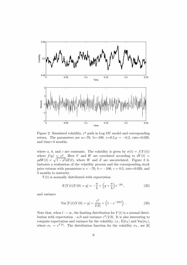
Figure 2: Simulated volatility, ey path in Log OU model and correspondingreturn. The parameters are a=-70, b=-100, c=0.5,ρ = −0.2, rate=0.029,and time=3 months.
where a, b, and c are constants. The volatility is given by σ(t) = f(Y (t))where f(y) = ey. Here V and W are correlated according to dV (t) =ρdW (t) +
√
1 − ρ2dZ(t), where W and Z are uncorrelated. Figure 2 il-lustrates a realization of the volatility process and the corresponding stockprice returns with parameters a = −70, b = −100, c = 0.5, rate=0.029, and3 months to maturity.
Y (t) is normally distributed with expectation
E [Y (t)|Y (0) = y] = −ab
+(
y +a
b
)
e−|b|t , (32)
and variance
Var [Y (t)|Y (0) = y] =c2
2 |b| +(
1 − e−2|b|t)
. (33)
Note that, when t→ ∞, the limiting distribution for Y (t) is a normal distri-bution with expectation −a/b and variance c2/2 |b|. It is also interesting tocompute expectation and variance for the volatility, i.e., E[σY ] and Var[σY ],where σY = eY (t). The distribution function for the volatility σY , see [6]
9
can be found to be
FσY(s) = P (σY ≤ s) = P (eY ≤ s) = P (Y ≤ log s) = FY (log s) , (34)
giving
fσY(s) =
d
dsFσY
(s) = fY (log s) · 1
s, (35)
The density function for Y is given by
fY (y) =1√2πσ
e−1
2(y−µ)2/σ2
, (36)
where µ=E[Y ] and σ2=Var[Y ] are given by equation (32) and (33). Thedensity function for σY is then given by
fσY(s) =
1
s√
2πσe−
1
2(log(s)−µ)2/σ2
, (37)
which is the density function for a lognormal distribution. The expectationfor the volatility is given by
E[
eY (t)]
= eµ+ 1
2σ2
, (38)
and the varianceVar
[
eY (t)]
= e2µ(
e2σ − eσ2)
. (39)
We will return to these models in Chapter 4.
3 The corrected pricing formula
In this section the corrected Black-Scholes price formula is derived. Theformula is general for all models with mean-reverting volatility and doesnot require estimation of the current volatility. The corrected Black-Scholesprice is given by
P = P0 − (T − t)
(
V2S2 ∂
2P0
∂S2+ V3S
3∂3P0
∂S3
)
, (40)
where P0 is the Black-Scholes price with constant volatility σ and (T − t)is the time to maturity. The parameters V2 and V3 will be computed laterfor a European call option. Formula (40) is not dependent on the choiceof volatility model, but in the present text the LogOU model is assumed.Before deriving the above formula, the concept of invariant distribution isreviewed.
10
3.1 Invariant distribution and important parameters
The invariant distribution of the stochastic process Y can be obtainedthrough finding an initial distribution for the process such that the processhas the same distribution at a later point in time. The invariant distribu-tion does not change in time and for Y the invariant distribution will be adistribution for Y (0) such that
E[Lg(Y (0))] = 0 , (41)
where L is the infinitesimal generator of the Y process. For the LogOUprocess it is given by
L = (a+ by)∂
∂y+
1
2c2∂2
∂y2. (42)
The density function for the invariant distribution for the LogOU process isgiven by, according to [2]
φ(y) =1√
2πν2exp
(
−(y −m)2
2ν2
)
, (43)
where m=−a/b and ν2=−c2/2b. The parameter b is the rate of mean re-version, and the inverse of b is the typical correlation time ε = −1/b. Thevariance ν2 controls the size of the fluctuations.
3.2 The pricing partial differential equation in terms of ε
The partial differential equation for the LogOU process can be written interms of ε
∂P ε
∂t+
1
2f(y)2S2∂
2P ε
∂S2+ν2
ε
∂2P ε
∂y2+ρν
√2√εSf(y)
∂2P ε
∂S∂y
+ r
(
S∂P ε
∂S− P ε
)
+
(
1
ε(m− y) − ν
√2√ε
Λ(y)
)
∂P ε
∂y= 0 , (44)
where m = −a/b and y is the current value of volatility level.It is convenient to write the partial differential equation above in terms
of the operators L0, L1, and L2(
1
εL0 +
1√εL1 + L2
)
P ε = 0 , (45)
where the operators are defined by
L0 = ν2 ∂2
∂y2+ (m− y)
∂
∂y,
L1 =√
2ρνSf(y)∂2
∂S∂y−
√2νΛ(y)
∂
∂y,
L2 = LBS(f(y)) =∂
∂t+
1
2f(y)2S2 ∂2
∂S2+ r
(
S∂
∂S− 1
)
,
(46)
11

where LBS is Black-Scholes operator.
3.3 Asymptotic solution
The solution P ε has a limit when ε goes to zero and the method used hereis to expand the solution P ε in powers of
√ε
P ε = P0 +√εP1 + εP2 + ε
√εP3 + . . . (47)
and subsequently solve for the coefficients P0, P1, P2, . . .. The terminal con-dition for P0 is the contract function h(S), i.e., P0(T, S, y) = h(S), and theterminal condition for Pi, i ≥ 1, is Pi(T, S, y) = 0. Inserting the expansion(47) into equation (45) and collecting powers of ε, the result is
1
εL0P0 +
1√ε(L0P1 + L1P0)
+ (L0P2 + L1P1 + L2P0)
+√ε(L0P3 + L1P2 + L2P1)
+ . . .
= 0 .
(48)
Step by step, the terms of order 1/ε, 1/√ε,. . . will be studied. The first term
in (48) isL0P0 = 0 . (49)
The operator L0 contains partial derivatives with respect to y but no deriva-tives with respect to S. One would therefore like to find a function whichis independent of y, P0 = P0(t, S) with terminal condition P0(T, S) = h(S).The next term in (48) is
L0P1 + L1P0 = 0 . (50)
It is known from above that P0 only depends on t and S, and L1 involvesderivatives with respect to y, yielding L1P0 = 0. The equation (50) is thusreduced to L0P1 = 0. The operator L0 involves derivatives with respect toy and one can once again search for a function which only depends on t andS, P1 = P1(t, S), with the terminal condition P1(T, S) = 0. When summingup, the two first terms in the expression (47) will not depend on y. Thenext term in order is the term of order 1,
L0P2 + L1P1 + L2P0 = 0 . (51)
It is known from the discussion above that P0 and P1 only depend on y, andthat L1 and L0 only involves derivatives with respect to y. Hence, L1P1 isequal to zero and equation (51) reduces to
L0P2 + L2P0 = 0 . (52)
12
Now, P0 is only dependent on t and S. When regarding S as fixed, L2P0 onlydepends on y, and equation (52) is a Poisson equation for P2 with respectto L0. In order to have a solution to the Poisson equation, L2P0 must be inthe orthogonal complement of the null space of L∗
0, where
L∗0 = ν2 ∂
2
∂y2+(a
b+ y) ∂
∂y+ 1 , (53)
and ν2=−c2/2b for the LogOU process. According to [7] this solvabilitycondition is equivalent to saying that L0P2 has mean zero with respect tothe invariant distribution, i.e.,
E [L2P0] = 〈L2P0〉 =
∫ ∞
−∞L2P0φ(y)dy = 0 , (54)
where φ in equation (43) solves L∗0φ = 0. The solvability condition above
requires that 〈L2P0〉 = 0. Because P0 does not depend on y the solvabilitycondition is reduced to
LBS(σ)P0 = 0 , (55)
where 〈L2〉 = LBS(σ) and σ is the effective volatility defined by
σ2 = E[
f(y)2]
= 〈f2〉 =
∫ ∞
−∞f(y)2φ(y)dy , (56)
which is the average with respect to the invariant distribution of Y .In conclusion, P0 is the solution of Black-Scholes equation with terminal
condition P0(T, S) = h(S) and σ = σ, where σ is given above.Equation (52) can be written as
L0P2 = −L2P0 . (57)
By applying the solvability condition in equation (54), L2P0 in the righthand side of (57) can be written as
L2P0 = L2P0 − 〈L2P0〉 =1
2
(
f(y)2 − σ2)
S2 ∂2P0
∂S2. (58)
Equation (57) is now given by
L0P2 = −1
2
(
f(y)2 − σ2)
S2∂2P0
∂S2. (59)
The solution of the Poisson equation in equation (59) is given by
P2 = −1
2L−1
0
(
f(y)2 − σ2)
S2∂2P0
∂S2(60)
= −1
2(ψ(y) + c(t, S)) S2 ∂
2P0
∂S2, (61)
13
where ψ(y) is a solution of the Poisson equation
L0ψ = f(y)2 − σ2 . (62)
Continuing to the next order, the terms of order√ε must also equal
zero, giving the equation
L0P3 + L1P2 + L2P1 = 0 . (63)
This is a Poisson equation for P3 with respect to L0. Moving L1P2+L2P1
to the right hand side of equation (63) gives
L0P3 = −(L1P2 + L2P1) . (64)
Again, applying the solvability condition in equation (54) we obtain
〈L1P2 + L2P1〉 = 0 . (65)
Here P2 is already known, so 〈L1P2〉 is moved to the right hand side to yield
〈L2P1〉 = −〈L1P2〉 , (66)
and now we investigate 〈L2P1〉. We note that P1 does not depend on yand 〈L2〉=LBS(σ) giving that the left hand side of equation (66) is equal toLBS(σ)P1. Focusing on the right hand side of (66), we find that
−〈L1P2〉 =1
2〈L1 (ψ(y) + c(t, S))〉S2∂
2P0
∂S2
=1
2〈L1ψ(y)〉S2 ∂
2P0
∂S2,
(67)
where ψ is a solution of the Poisson equation (62). The result of the discus-sion above is that the solvability condition yields the equation
LBS(σ)P1 =1
2〈L1ψ(y)〉S2 ∂
2P0
∂S2. (68)
We compute, for a general function ϕ,
〈L1ψ(y)ϕ(S)〉 =
⟨(√2ρνSf(y)
∂2
∂S∂y−
√2νΛ(y)
∂
∂y
)
(ψ(y)ϕ(S))
⟩
=√
2ρνS⟨
f(y)ψ′(y)⟩ ∂
∂Sϕ(S) −
√2ν⟨
Λ(y)ψ′(y)⟩
ϕ(S)
(69)
Inserting the above expression into equation (68) gives
LBS(σ)P1 =1
2
(√2ρνS
⟨
f(y)ψ′(y)⟩ ∂
∂S−
√2ν⟨
Λ(y)ψ′(y)⟩
)
S2∂2P0
∂S2
=
√2
2ρν⟨
f(y)ψ(y)′⟩
S3 ∂3P0
∂S3
+
(
√2ρν
⟨
f(y)ψ(y)′⟩
−√
2
2ν⟨
Λ(y)ψ(y)′⟩
)
S2∂2P0
∂S2,
(70)
14
and the terminal condition is P1(T, S) = 0. Following Fouque [2], the firstcorrection is denoted by
P1(t, S) =√εP1(t, S) , (71)
which is a solution ofLBS(σ)P1 = H(t, S) , (72)
and the terminal condition P1(T, S) = 0. Here H(t, S) is defined by
H(t, S) = V2S2 ∂
2P0
∂S2+ V3S
3∂3P0
∂S3, (73)
where
V2 =ν√−2b
(
2ρ〈fψ′〉 − 〈Λψ′〉)
,
V3 =ρν√−2b
〈fψ′〉 .(74)
It can be shown, see [2], that equation (72) together with the terminalcondition has the solution
P1(t, S) = −(T − t)H(t, S) . (75)
Finally, the corrected Black-Scholes price is given by
P ' P0 + P1 = P0 − (T − t)
(
V2S2 ∂
2P0
∂S2+ V3S
3∂3P0
∂S3
)
. (76)
3.4 Expression for V2 and V3
In this section the calculations of V2 and V3 in terms of the model param-eters for the Log Ornstein-Uhlenbeck and Cox-Ingersoll-Ross model will bepresented. The expression for V2 and V3 in equation (74) can equivalentlybe written as, compare [2],
V2 =1
ν√−2b
⟨[
−2ρF + ρ(µ− r)F +√
1 − ρ2M]
(
f2 − 〈f2〉)
⟩
,
V3 =−ρ
ν√−2b
⟨
F(
f2 − 〈f2〉)⟩
,(77)
where F, F and M are primitive functions of f, 1/f and γ. So far the specificchoice of model is not important. However, to proceed further it is necessaryto specify f(y).
15
3.4.1 Log Ornstein-Uhlenbeck
In order to calculate the expectation values in equation (77) the invariantdistribution is needed. For the LogOU model it is given by
φ(y) =1√2πν
e−(y−m)2/2ν2
, (78)
where m = −a/b and ν2 = c2/2 |b|. As mention before, in this modelf(y) = ey. By using the expression for V2 given in equation (77) and theexplicit expression for φ and f we obtain
V2 =1
c
⟨[
−2ρey − ρ(µ− r)e−y +√
1 − ρ2M]
(
e2y − 〈e2y〉)
⟩
=1
c
∫ ∞
−∞
([
−2ρey − ρ(µ− r)e−y +√
1 − ρ2M]
(
e2y − 〈e2y〉)
)
φ(y)dy
=−2ρ
c
(
e9ν2/2+3m − e5ν2/2+3m)
− ρ
c(µ− r)
(
eν2/2+m − e5ν2/2+m
)
+2√−2b
√
1 − ρ2γσ2ν .
(79)
Similarly V3 can been calculated, starting from V3 in equation (77)
V3 =−ρc
⟨
ey(
e2y − 〈e2y〉)⟩
=−ρc
∫ ∞
−∞ey(
e2y − 〈e2y〉)
φ(y)dy
=−ρc
(
e9ν2/2+3m − e5ν2/2+3m)
.
(80)
3.4.2 Cox-Ingersoll-Ross
In this model Y (t) has a non-central chi-square distribution and the invariantdistribution is given by a gamma distribution
ξ(y) =y(α−1)e−(y/β)
Γ(α)βα, y > 0 (81)
where α = 2a/c2 and β = −c2/2b . Using equation (77) and f(y) =√y, V2
can be calculated as
V2 =1
β√−2bα
⟨[
−4
3ρy3/2 + 2ρ(µ− r)
√y +
√
1 − ρ2γy
]
(y − 〈y〉)⟩
=1
β√−2bα
∫ ∞
0
[
−4
3ρy3/2 + 2ρ(µ− r)
√y +
√
1 − ρ2γy
]
(y − αβ) ξ(y)dy
=1√
−2bα
(
αβγ√
1 − ρ2 +Γ(
12 + α
)
Γ (α)
√
βρ [(µ− r) − β(1 − 2α)]
)
.
(82)
16
Similar calculations for V3 yield
V3 =−ρ
β√−2bα
〈√y (y − 〈y〉)〉
=−ρ
β√−2bα
∫ ∞
0
√y (y − αβ) ξ(y)dy
=−ρβ3/2
√−2bα
Γ(
32 + α
)
Γ (α),
(83)
3.5 Implied volatility for a European call option
In this section the implied volatility for a European call option will be calcu-lated in terms of V2 and V3. The implied volatility is computed by solving therelation between theoretical and observed price given in equation (1) withrespect to the implied volatility I. The approximating price is, accordingto the discussion above, given by P0+P1, where P0 = CBS . Black-Scholesformula for a call option is given in Appendix by (121), d1 and d2 are givenby (122) and (123), in this case is σ the effective volatility σ. In order toapply the approximative solution (76) it is necessary to calculate the secondand third derivative of P0 with respect to S. The first derivative is knownas Delta,
∂P0
∂S= N(d1) , (84)
and the second derivative is called Gamma,
∂2P0
∂S2=
ed2
1/2
Sσ√
2π(T − t). (85)
Fouque, see [2] introduced a new ”Greek” called Epsilon, defined as the thirdderivative,
∂3P0
∂S3=
−ed2
1/2
S2σ√
2π(T − t)
(
1 +d1
σ√
(T − t)
)
. (86)
Equation (73) gives
H(t, S) =Sed
2
1/2
σ√
2π(T − t)
(
V2 − V3 −V3d1
σ√
(T − t)
)
, (87)
and the expression for P1(t, S) is
P1(t, S) =Sed
2
1/2
σ√
2π
(
V3d1
σ+ (V3 − V2)
√T − t
)
. (88)
Taking the corrected pricing formula as the observed price, Cobs(K,T ) =P0(t, S) + P1(t, S) in equation (1), the relation that determines the impliedvolatility is thus
CBS(t, S,K, T, I) = P0 + P1 . (89)
17
Equation (89) can be solved by expanding I as I = σ +√εI1 + · · · , and
inserting this in the left hand side of (89). The implied volatility is thengiven by
I = σ + P1(t, S)
[
∂CBS
∂σ(t, S,K, T, σ)
]−1
+ O(1/α) . (90)
The derivative of the Black-Scholes price with respect to σ is the Vega,
∂CBS
∂σ=Sed
2
1/2√T − t√
2π. (91)
When putting (88), (91), and d1 into equation (90) the implied volatilitycan be written as
I = σ +V3
σ3
(
r +3
2σ2
)
− V2
σ− V3
σ3
(
log(KS )
T − t
)
+ O(1/α) . (92)
The implied volatility is given in terms of strike price K, asset price S, timeto maturity T − t, and the parameters A1 and A2 as the following
I = A1
[
log(
KS
)
T − t
]
+A2 + O(1/α) , (93)
where A1 and A2 are defined as
A1 = −V3
σ3,
A2 = σ +V3
σ3
(
r +3
2σ2
)
− V2
σ.
(94)
The parameters V2 and V3 are given by
V2 = σ
(
(σ −A2) −A1
(
r +3
2σ2
))
,
V3 = −A1σ3 .
(95)
The formula for the implied volatility given in equation (93) is not validwhen the time to maturity is short or if the option is far out of money. Onereason is that the Y (t) process does not have sufficient time to mean-revertmany times.
4 Simulation and estimation
In this chapter simulation methods, results from the simulations and pa-rameter estimations will be presented. It is important to note that thecalculations are done directly in the probability measure Q. The marketprice of risk is thus assumed to be zero. Common for all studied modelsare that the implied volatility has been calculated and plotted against strikeprice. In all cases it has resulted in smile curves.
18
0.8 0.85 0.9 0.95 1 1.05 1.1 1.15 1.2 1.25 1.3
0.2
0.4
0.6
0.8
1
1.2
Strike Price/Current Price
Impl
ied
Vol
atili
ty
Figure 3: Observed implied volatility for OMX call option (with circles) andSkandia call option (with stars).
4.1 Examples from the Swedish option market
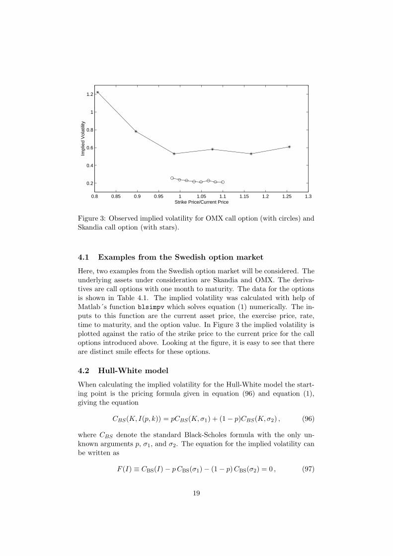
Here, two examples from the Swedish option market will be considered. Theunderlying assets under consideration are Skandia and OMX. The deriva-tives are call options with one month to maturity. The data for the optionsis shown in Table 4.1. The implied volatility was calculated with help ofMatlab´s function blsimpv which solves equation (1) numerically. The in-puts to this function are the current asset price, the exercise price, rate,time to maturity, and the option value. In Figure 3 the implied volatility isplotted against the ratio of the strike price to the current price for the calloptions introduced above. Looking at the figure, it is easy to see that thereare distinct smile effects for these options.
4.2 Hull-White model
When calculating the implied volatility for the Hull-White model the start-ing point is the pricing formula given in equation (96) and equation (1),giving the equation
CBS(K, I(p, k)) = pCBS(K,σ1) + (1 − p)CBS(K,σ2) , (96)
where CBS denote the standard Black-Scholes formula with the only un-known arguments p, σ1, and σ2. The equation for the implied volatility canbe written as
F (I) ≡ CBS(I) − pCBS(σ1) − (1 − p)CBS(σ2) = 0 , (97)
19
Skandia Strike price Option price Implied volatility
Current price:22.30 18 5.50 1.22Time:1 month 20 3.30 0.78
Rate:0.035 22 1.55 0.5324 0.85 0.5826 0.30 0.5328 0.20 0.61
OMX Strike price Option price Implied volatility
Current price:590.90 580 25.00 0.26Time:1 month 590 18.00 0.24
Rate:0.029 600 12.80 0.23610 8.25 0.22620 5.25 0.21630 3.90 0.23640 2.00 0.21650 1.15 0.21
Table 1: Strike price, option price, implied volatility, current asset price,rate and time to maturity for Skandia and OMX call options.
which can be solved with respect to I. Equation (97) can be solved byusing some numerical method, e.g., the Newton-Raphson method or one ofMatlab´s solver functions. The iterative scheme for the numerical solutionusing Newton-Raphson is
In+1 = In − F (In)
V(In), (98)
where
V =∂F
∂I=∂CBS
∂I. (99)
In the results as follows, Matlab’s solver function fzero has been used andthe parameters in the model are arbitrary chosen. The next step is to plotthe implied volatility for different values of the strike price, which results ina smile shaped curve. It is interesting to vary parameters in the model andinvestigate what happen with the smile curve.
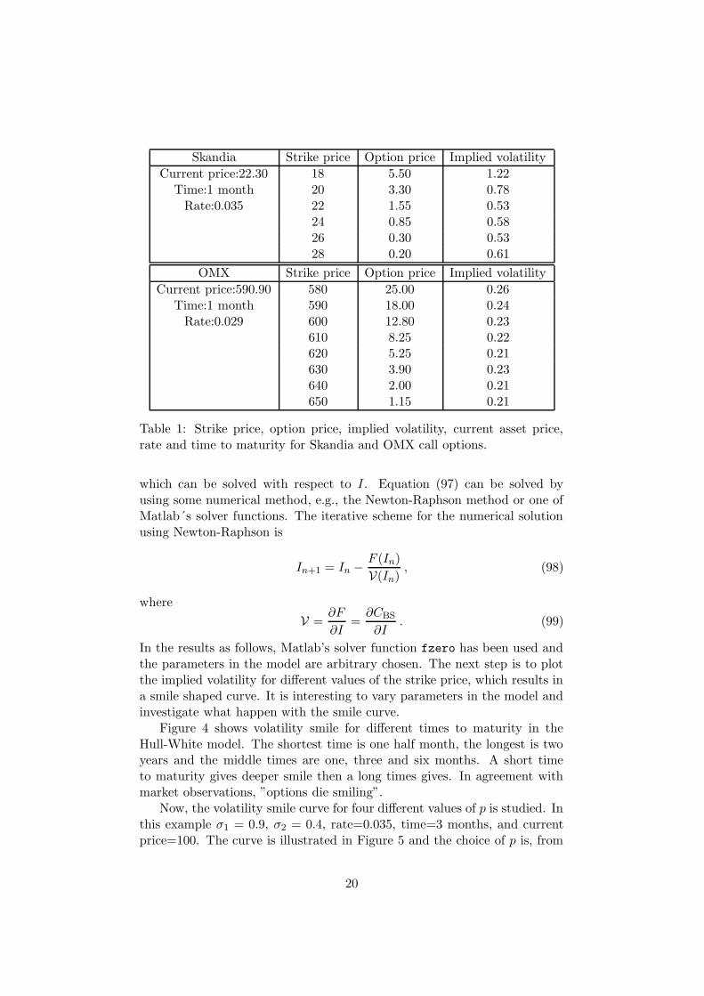
Figure 4 shows volatility smile for different times to maturity in theHull-White model. The shortest time is one half month, the longest is twoyears and the middle times are one, three and six months. A short timeto maturity gives deeper smile then a long times gives. In agreement withmarket observations, ”options die smiling”.
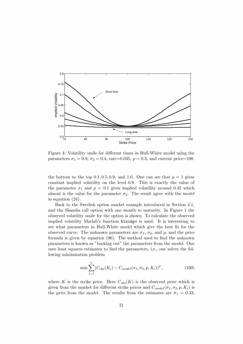
Now, the volatility smile curve for four different values of p is studied. Inthis example σ1 = 0.9, σ2 = 0.4, rate=0.035, time=3 months, and currentprice=100. The curve is illustrated in Figure 5 and the choice of p is, from
20
70 80 90 100 110 120 1300.5
0.55
0.6
0.65
0.7
0.75
0.8
Strike Price
Impl
ied
Vol
atili
ty
Short time
Long time
Figure 4: Volatility smile for different times in Hull-White model using theparameters σ1 = 0.9, σ2 = 0.4, rate=0.035, p = 0.3, and current price=100.
the bottom to the top 0.1, 0.5, 0.9, and 1.0. One can see that p = 1 givesconstant implied volatility on the level 0.9. This is exactly the value ofthe parameter σ1 and p = 0.1 gives implied volatility around 0.45 whichalmost is the value for the parameter σ2. The result agree with the modelin equation (24).
Back to the Swedish option market example introduced in Section 4.1,and the Skandia call option with one month to maturity. In Figure 1 theobserved volatility smile for the option is shown. To calculate the observedimplied volatility Matlab’s function blsimpv is used. It is interesting tosee what parameters in Hull-White model which give the best fit for theobserved curve. The unknown parameters are σ1, σ2, and p, and the priceformula is given by equation (96). The method used to find the unknownparameters is known as ”backing out” the parameters from the model. Oneuses least squares estimates to find the parameters, i.e., one solves the fol-lowing minimization problem
min
n∑
i=1
(Cobs(Ki) − Cmodel(σ1, σ2, p,Ki))2 , (100)
where K is the strike price. Here Cobs(K) is the observed price which isgiven from the market for different strike prices and Cmodel(σ1, σ2, p,Ki) isthe price from the model. The results from the estimates are σ1 = 0.33,
21
70 80 90 100 110 120 1300.4
0.5
0.6
0.7
0.8
0.9
1Im
plie
d V
olat
ility
Strike Price
p=0.1p=0.5p=0.9p=1.0
p=0.1p=0.5p=0.9p=1.0
p=0.1p=0.5p=0.9p=1.0
Figure 5: Volatility smile for different p values using the parameters σ1 = 0.9,σ2 = 0.4, rate=0.035, time=3 months, and current price=100.
σ2 = 9.2, and p = 0.97. In Figure 6 the observed volatility smile is com-pared to the model. The modeled smile is calculated using the estimatedparameters. The results shows that the ”backed out” parameter are not sogood estimates, perhaps depending insufficient data.
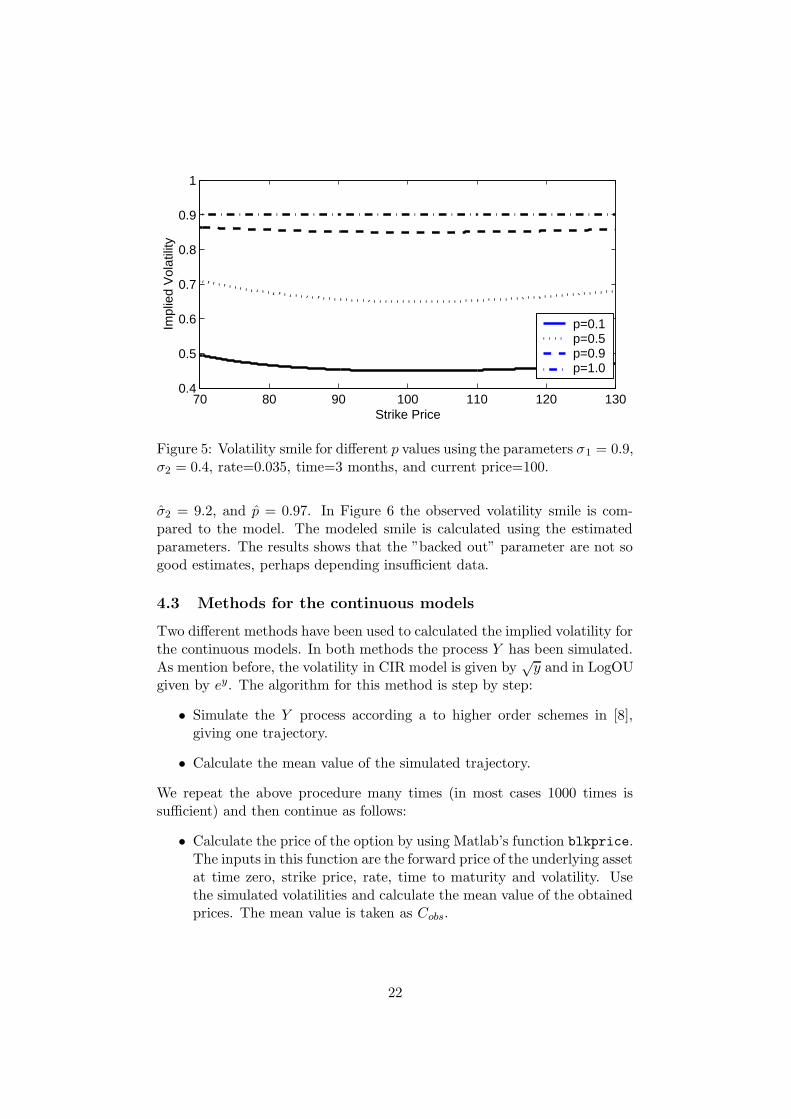
4.3 Methods for the continuous models
Two different methods have been used to calculated the implied volatility forthe continuous models. In both methods the process Y has been simulated.As mention before, the volatility in CIR model is given by
√y and in LogOU
given by ey. The algorithm for this method is step by step:
• Simulate the Y process according a to higher order schemes in [8],giving one trajectory.
• Calculate the mean value of the simulated trajectory.
We repeat the above procedure many times (in most cases 1000 times issufficient) and then continue as follows:
• Calculate the price of the option by using Matlab’s function blkprice.The inputs in this function are the forward price of the underlying assetat time zero, strike price, rate, time to maturity and volatility. Usethe simulated volatilities and calculate the mean value of the obtainedprices. The mean value is taken as Cobs.
22
0.6 0.7 0.8 0.9 1 1.1 1.2 1.3 1.40.5
0.6
0.7
0.8
0.9
1
1.1
1.2
1.3
Strike Price/Current Price
Impl
ied
Vol
atili
ty
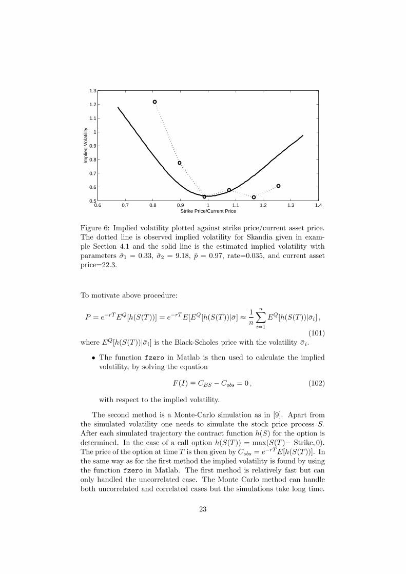
Figure 6: Implied volatility plotted against strike price/current asset price.The dotted line is observed implied volatility for Skandia given in exam-ple Section 4.1 and the solid line is the estimated implied volatility withparameters σ1 = 0.33, σ2 = 9.18, p = 0.97, rate=0.035, and current assetprice=22.3.
To motivate above procedure:
P = e−rTEQ[h(S(T ))] = e−rTE[EQ[h(S(T ))|σ] ≈ 1
n
n∑
i=1
EQ[h(S(T ))|σi] ,
(101)where EQ[h(S(T ))|σi] is the Black-Scholes price with the volatility σi.
• The function fzero in Matlab is then used to calculate the impliedvolatility, by solving the equation
F (I) ≡ CBS − Cobs = 0 , (102)
with respect to the implied volatility.
The second method is a Monte-Carlo simulation as in [9]. Apart fromthe simulated volatility one needs to simulate the stock price process S.After each simulated trajectory the contract function h(S) for the option isdetermined. In the case of a call option h(S(T )) = max(S(T )− Strike, 0).The price of the option at time T is then given by Cobs = e−rTE[h(S(T ))]. Inthe same way as for the first method the implied volatility is found by usingthe function fzero in Matlab. The first method is relatively fast but canonly handled the uncorrelated case. The Monte Carlo method can handleboth uncorrelated and correlated cases but the simulations take long time.
23

80 85 90 95 100 105 110 115 1200.66
0.67
0.68
0.69
0.7
0.71
0.72
0.73
0.74
0.75
0.76
Strike Price
Impl
ied
Vol
atili
ty
Short time
Long time
Figure 7: Volatility smile for different times in CIR model, a=50, b=-100,c=40, rate=0.035, and current price=100.
The last method can be more effective when using variance reduction, see[9].
It is also interesting to estimate which values of the parameter that givethe best fit to the observed volatility smile. One should be able to use thesame method as in the previous section. However we have not done this dueto lack of time.
4.4 Cox-Ingersoll-Ross model
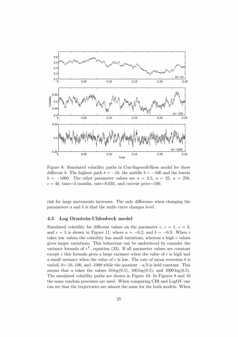
We study what happens with the volatility trajectory when the parametersa, b, and c in this model change. From Section 2.2.2, it is known that theparameter −b is the rate of mean reversion. Results of simulated pathswhen the parameter b takes three different values are shown in Figure 8,the chosen values of b are −10, −100, and −1000. The quotient −a/b isheld constant, which results in that a takes the values 2.5, 25, and 250. Therandom processes are the same in the three different realizations. One cansee that b with the smallest absolute value gives the highest path. Highabsolute value of b press down the path, giving small fluctuations aroundthe mean −a/b.
Volatility smiles for different times for the CIR model is shown in Figure7. The parameters are a = 50, b = −100 and c = 40. What happen withthe smile when, for example, the parameter c is smaller than 40 ? Wecompare four different values, c = 10, c = 20, c = 30, and c = 40 which arearbitrarily chosen. The result is that a small c gives a flatter smile than alarge c, see Figure 9. One reasonable explanation to this can be that thedensity function for the stock price has fatter tails. Fat tails means that the
24
0 0.05 0.10 0.15 0.20 0.25 0.4
0.45
0.5
0.55
Vol
atili
ty
0 0.05 0.10 0.15 0.20 0.25 0.2
0.3
0.4
0.5
0.6
0 0.05 0.10 0.15 0.20 0.25 0.45
0.5
0.55
Time
b=−10
b=−100
b=−1000
Figure 8: Simulated volatility paths in Cox-Ingersoll-Ross model for threedifferent b. The highest path b = −10, the middle b = −100 and the lowestb = −1000. The other parameter values are a = 2.5, a = 25, a = 250,c = 40, time=3 months, rate=0.035, and current price=100.
risk for large movements increases. The only difference when changing theparameters a and b is that the smile curve changes level.
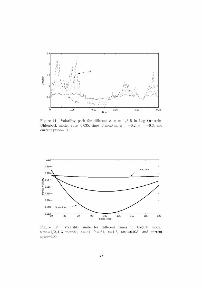
4.5 Log Ornstein-Uhlenbeck model
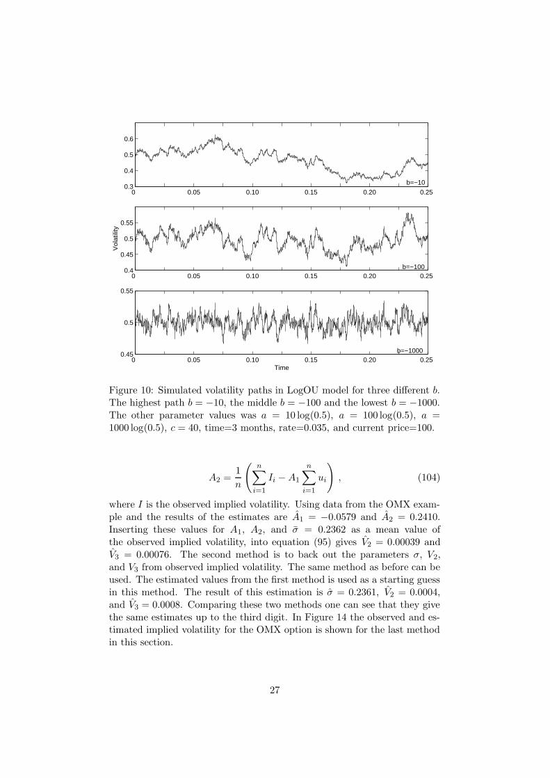
Simulated volatility for different values on the parameter c, c = 1, c = 3,and c = 5 is shown in Figure 11, where a = −0.2, and b = −0.3. When ctakes low values the volatility has small variations, whereas a high c valuesgives larger variations. This behaviour can be understood by consider thevariance formula of eY , equation (33). If all parameter values are constantexcept c this formula gives a large variance when the value of c is high anda small variance when the value of c is low. The rate of mean reversion b isvaried, b=-10,-100, and -1000 while the quotient −a/b is held constant. Thismeans that a takes the values 10 log(0.5), 100 log(0.5), and 1000 log(0.5).The simulated volatility paths are shown in Figure 10. In Figures 8 and 10the same random processes are used. When comparing CIR and LogOU onecan see that the trajectories are almost the same for the both models. When
25

80 85 90 95 100 105 110 115 1200.66
0.67
0.68
0.69
0.7
0.71
0.72
0.73
0.74
0.75
Strike Price
Impl
ied
Vol
atili
ty
c=10c=20c=30c=40
Figure 9: Volatility smile for different c values in CIR using the parametersa = 50, b = −100, rate=0.035, time=1/2 month, and current price=100.
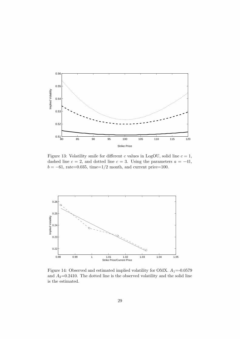
looking at the volatility smile for different times in Log Ornstein-Uhlenbeckmodel, it can be seen that a short time to maturity gives a deeper smile thena long time gives, which is illustrated in Figure 12. The results of changingthe parameters a and b gives only a change in level, but different values ofc gives changes in the shape. High values gives a deeper smile than lowvalues, which is illustrated, Figure 13 shows this smiles. The explanation tothis behavior is the same as in CIR model, see above.
4.6 Estimated V2 and V3
In equation (93) in Section 3.5 the formula for the implied volatility for aEuropean call option is given. With help of historical price data, A1 and A2
in this formula can be estimated. The straight forward method proposed in[2] is to estimate A1 and A2 from observed implied volatility. This can bedone with least squares estimate. Put ui = (log(K(i)/S))/(T − t) where Kis the strike price, S is the stock price, and T − t is the time to maturity.Then A1 and A2 are given by
A1 =1n (∑n
i=1 Ii∑n
i=1 ui) −∑n
i=1 Iiui
1n (∑n
i=1 ui)2 −∑n
i=1 u2i
, (103)
26
0 0.05 0.10 0.15 0.20 0.25 0.3
0.4
0.5
0.6
0 0.05 0.10 0.15 0.20 0.25 0.4
0.45
0.5
0.55
Vol
atili
ty
0 0.05 0.10 0.15 0.20 0.25 0.45
0.5
0.55
Time
b=−10
b=−100
b=−1000
Figure 10: Simulated volatility paths in LogOU model for three different b.The highest path b = −10, the middle b = −100 and the lowest b = −1000.The other parameter values was a = 10 log(0.5), a = 100 log(0.5), a =1000 log(0.5), c = 40, time=3 months, rate=0.035, and current price=100.
A2 =1
n
(
n∑
i=1
Ii −A1
n∑
i=1
ui
)
, (104)
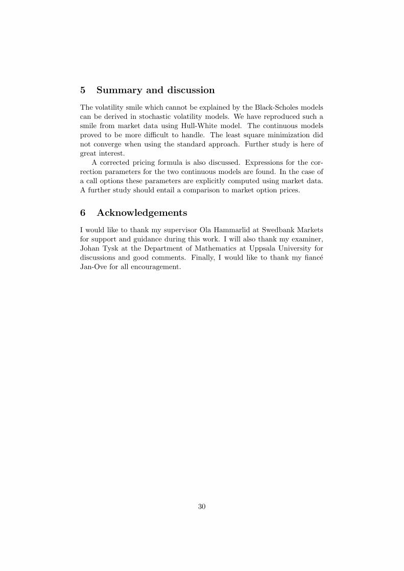
where I is the observed implied volatility. Using data from the OMX exam-ple and the results of the estimates are A1 = −0.0579 and A2 = 0.2410.Inserting these values for A1, A2, and σ = 0.2362 as a mean value ofthe observed implied volatility, into equation (95) gives V2 = 0.00039 andV3 = 0.00076. The second method is to back out the parameters σ, V2,and V3 from observed implied volatility. The same method as before can beused. The estimated values from the first method is used as a starting guessin this method. The result of this estimation is σ = 0.2361, V2 = 0.0004,and V3 = 0.0008. Comparing these two methods one can see that they givethe same estimates up to the third digit. In Figure 14 the observed and es-timated implied volatility for the OMX option is shown for the last methodin this section.
27
0 0.05 0.10 0.15 0.20 0.250
0.5
1
1.5
2
2.5
Time
Vol
atili
ty
c=5
c=1
Figure 11: Volatility path for different c, c = 1, 3, 5 in Log Ornstein-Uhlenbeck model, rate=0.035, time=3 months, a = −0.2, b = −0.3, andcurrent price=100.
80 85 90 95 100 105 110 115 1200.512
0.513
0.514
0.515
0.516
0.517
0.518
0.519
0.52
Strike Price
Impl
ied
Vol
atili
ty
Long time
Short time
Figure 12: Volatility smile for different times in LogOU model,time=1/2, 1, 3 months, a=-41, b=-61, c=1.2, rate=0.035, and currentprice=100.
28
80 85 90 95 100 105 110 115 1200.51
0.52
0.53
0.54
0.55
0.56
Strike Price
Impl
ied
Vol
atili
ty
Figure 13: Volatility smile for different c values in LogOU, solid line c = 1,dashed line c = 2, and dotted line c = 3. Using the parameters a = −41,b = −61, rate=0.035, time=1/2 month, and current price=100.
0.98 0.99 1 1.01 1.02 1.03 1.04 1.05
0.22
0.23
0.24
0.25
0.26
Strike Price/Current Price
Impl
ied
Vol
atili
ty
Figure 14: Observed and estimated implied volatility for OMX. A1=-0.0579and A2=0.2410. The dotted line is the observed volatility and the solid lineis the estimated.
29
5 Summary and discussion
The volatility smile which cannot be explained by the Black-Scholes modelscan be derived in stochastic volatility models. We have reproduced such asmile from market data using Hull-White model. The continuous modelsproved to be more difficult to handle. The least square minimization didnot converge when using the standard approach. Further study is here ofgreat interest.
A corrected pricing formula is also discussed. Expressions for the cor-rection parameters for the two continuous models are found. In the case ofa call options these parameters are explicitly computed using market data.A further study should entail a comparison to market option prices.
6 Acknowledgements
I would like to thank my supervisor Ola Hammarlid at Swedbank Marketsfor support and guidance during this work. I will also thank my examiner,Johan Tysk at the Department of Mathematics at Uppsala University fordiscussions and good comments. Finally, I would like to thank my fianceJan-Ove for all encouragement.
30
A Appendix
A.1 Basic arbitrage theory
In this section Wiener processes will be described. A a more comprehensivediscussion of the basic arbitrage theory can be found in reference [1].
A stochastic process W is called a Wiener process if the following con-ditions hold:
1. W (0) = 0.
2. The process W has independent increments, i.e., if r < s ≤ t < u thenW (u) −W (t) and W (s) −W (r) are independent stochastic variables.
3. For s < t the stochastic variableW (t)−W (s) has Gaussian distributionN(0,
√t− s)
4. W has continuous trajectories.
The Black-Scholes model consists of two assets, one risk-less B and onestock S with following dynamics
dB(t) = rB(t)dt (105)
dS(t) = αS(t)dt + σS(t)dW (t) (106)
where r, α, and σ is the rate, the drift, and the volatility, respectively. Themodel is complete because it contains one traded asset, S and one randomsources, W (t). The price at time t for the option is given by F (t, S(t)). Thedifferential dF can be found by using Ito’s lemma
dF =
(
∂F
∂t+ αS
∂F
∂S+
1
2σ2S2∂
2F
∂S2
)
dt+∂F
∂SσSdW . (107)
By introducing the quantities
αf ≡ 1
F
(
∂F
∂t+ αS
∂F
∂S+
1
2σ2S2∂
2F
∂S2
)
, (108)
and
σf =σS
F
∂F
∂S, (109)
the differential may be written as
dF = αfFdt+ σfFdW . (110)
Form a risk-less portfolio with the underlying stock and the option. Π isvalue of this portfolio and dΠ is the differential. A risk-less portfolio is
31
obtained when the dW term in the differential vanish. If Π is self-financingwe obtain the following dynamics
dΠ = Π
(
ns∂S
S+ nf
∂F
F
)
= Π [(nsα+ nfαf )dt+ (nsσ + nfσf )dW ] (111)
where ns is the relative part in stock and nf is the relative part in option.From the risk-less criterion and that ns and nf are relative parts of thewhole portfolio the following equations must hold
nsσ + nfσf = 0 , (112)
ns + nf = 1 . (113)
The linear system in (112) has the solution
ns =σf
σf − σ, (114)
nf =−σ
σf − σ. (115)
The portfolio is arbitrage free if
nsα+ nfαf = r . (116)
Inserting ns, nf , and αf into equation (116) and multiplying by (σf − σ)Fone obtains
σfFα− σ
(
∂F
∂t+ αS
∂F
∂S+
1
2σ2S2 ∂
2F
∂S2
)
= (σf − σ) rF . (117)
By using (109) in (117) the following partial differential equation governingthe price of the option is obtained,
∂F
∂t+ rS
∂F
∂S+
1
2σ2S2∂
2F
∂S2= rF . (118)
With the above results the Black-Scholes equation can be formulated as
∂F
∂t+ rS
∂F
∂S+
1
2σ2S2 ∂
2F
∂S2− rF = 0 , (119)
F (T, S) = h(S) , (120)
where F (T, S) is the price of the option at time T , when the underlyingasset has the price S, and h(S) is the contract function.
The Black-Scholes equation can be solved analytically and the price ofa European call option with strike price K and time of maturity T is givenby C(t, S(t)), where
CBS(t, S) = SN(d1) −Ke−r(T−t)N(d2) , (121)
32

where
d1 =log(S/K) + (r + 1/2σ2)(T − t)
σ√T − t
, (122)
d2 = d1 − σ√T − t , (123)
and
N(z) =1√2π
∫ z
−∞e−y2/2dy . (124)
Here N(z) is the cumulative distribution of a normal random variable, withmean 0 and variance 1.
The contract function for the European call option is given by
h(S) = max(S −K, 0) , (125)
where h(S) gives the value of the option at expiration. If the strike priceis lower than the underlying stock price at expiration the value of h(S) islarger than zero and the profit will be S −K. The other possible situationis that the strike price is higher than the underlying stock price, in whichcase the value of the contract function is zero and the option is worthless.The contract function for the European put option is given by
h(S) = max(K − S, 0) (126)
and the discussion above is contrary.
33
References
[1] Bjork Tomas. Arbitrage theory in continuous time. Oxford universitypress, Oxford, 1998.
[2] Fouque Jean-Pierre, Papanicolaou George, and Sircar K. Ronnie. Deriva-
tives in financial markets with stochastic volatility. Cambridge universitypress, Cambridge, 2000.
[3] Hull John and White Alan. The pricing of options on assets with stochas-tic volatilities. J. Finance, 42(2):281–300, 1987.
[4] Renault E. and Touzi N. Option hedging and implied volatilities in astochastic volatility model. Math.Finance, 6(3):279–302, 1996.
[5] Hull John and White Alan. Hull-White on derivatives. Risk Publications,London, 1996.
[6] Gut Allan. An Intermediate Curse in Probability. Springer-Verlag, NewYork, 1995.
[7] Fouque Jean-Pierre and Papanicolaou George and Sircar K. Ronnie.Mean-reverting stochastic volatility. International Journal of theoreti-
cal and applied finance, 3(1):101–142, 2000.
[8] Asmussen Søren. Stochastic simulation with a view towards stochasticprocesses. http://www.maphysto.dk, July, 2003.
[9] Luenberger David G. Inverstment Science. Oxford university press, NewYork, 1998.
34