Stochastic interpretation of the advection diﬀusion...

JOURNAL OF GEOPHYSICAL RESEARCH, VOL. ???, XXXX, DOI:10.1002/,

Stochastic interpretation of the advection diffusion equation and

its relevance to bed load transport

C. Ancey1, P. Bohorquez2, and J. Heyman1

Abstract. The advection diffusion equation is one of the most widespread equationsin physics. It arises quite often in the context of sediment transport, e.g., for describ-ing time and space variations in the particle activity (the solid volume of particles inmotion per unit streambed area). Phenomenological laws are usually sufficient to derivethis equation and interpret its terms. Stochastic models can also be used to derive it,with the significant advantage that they provide information on the statistical proper-ties of particle activity. These models are quite useful when sediment transport exhibitslarge fluctuations (typically at low transport rates), making the measurement of meanvalues difficult. Among these stochastic models, the most common approach consists ofrandom walk models. For instance, they have been used to model the random displace-ment of tracers in river streams. Here we explore an alternative approach, which involvesmonitoring the evolution of the number of particles moving within an array of cells offinite length. Birth-death Markov processes are well-suited to this objective. While thetopic has been explored in detail for diffusion-reaction systems, the treatment of advec-tion has received no attention. We therefore look into the possibility of deriving the ad-vection diffusion equation (with a source term) within the framework of birth-death Markovprocesses. We show that in the continuum limit (when the cell size becomes vanishinglysmall), we can derive an advection diffusion equation for particle activity. Yet, while thisderivation is formally valid in the continuum limit, it runs into difficulty in the practi-cal applications involving cells or meshes of finite length. Indeed, within our stochasticframework, particle advection produces nonlocal effects, which are more or less signif-icant depending on the cell size and particles’ velocity. Albeit nonlocal, these effects looklike (local) diffusion and add to the intrinsic particle diffusion (dispersal due to veloc-ity fluctuations), with the important consequence that local measurements depend onboth the intrinsic properties of particles’ displacement and the dimensions of the mea-surement system.

1. Introduction

This article is concerned with the microscopic foundationof the advection diffusion equation with a source term

∂c

∂t+ up

∂c

∂x= s(c) +D

∂2c

∂x2. (1)

As we will mainly study this equation in the context of sedi-ment transport, c(x, t) denotes the solid volume of particlesin motion per unit streambed area [m]. Following Furbishet al. [2012a], we refer to c as particle activity. We will focuson one-dimensional problems and so c is expressed as a func-tion of the position x along the streambed and time t. Thesecond term on the left-hand side represents advection andup is the advection velocity [m s−1], i.e., the mean velocity ofparticles when sediment is in motion. The first contributionto the right-hand side represents the source term, here thenet balance between the entrainment and deposition ratesof particles from/on a stream bed. In this paper, we willfocus on linear processes, and so we assume that the source

1School of Architecture, Civil and EnvironmentalEngineering, Ecole Polytechnique Federale de Lausanne,1015 Lausanne, Switzerland

2Ingenierıa Mecanica y Minera, Universidad de Jaen,23071 Jaen, Spain

Copyright 2015 by the American Geophysical Union.0148-0227/15/$9.00

term s [m s−1] is either independent of c or a linear functionof c (see section 2.2). The second term on the right-handside of equation (1) is the diffusion process, with D the par-ticle diffusivity [m s−2]. The physical interpretation of theadvection diffusion equation (1) is straightforward: particleactivity varies with time as a result of transport by the waterstream (advection), spreading (dispersion or diffusion due toparticles’ velocity fluctuations), and mass transfer with thestream bed (entrainment and deposition).

The advection diffusion equation is one of the mostwidespread equations in physics and related sciences. InEarth surface processes related to sediment transport, itarises in different forms and in various contexts such as soilcreep and erosion [Culling , 1960; Furbish and Haff , 2010],landscape evolution [Paola, 2000; Martin, 2000; Tucker andBradley , 2010; Salles and Duclaux , 2015], bed load transport[Parker et al., 2000; Lajeunesse et al., 2010; Furbish et al.,2012b; Ancey and Heyman, 2014; Pelosi et al., 2014], sus-pended transport [van Rijn, 2007], solute transport [Bencalaand Walters, 1983; Boano et al., 2007], and wave-inducedsediment transport [Blondeaux et al., 2012]. Diffusion is alsoat the core of many investigations on suspension and bedloadtransport [Oh and Tsai , 2010; Seizilles et al., 2014], hills-lope sediment transport [Heimsath et al., 2005; Foufoula-Georgiou et al., 2010], evolution of braiding rivers [Reitzet al., 2014], and tracer behavior [Nikora et al., 2002; Gantiet al., 2010; Martin et al., 2012; Roseberry et al., 2012; La-jeunesse et al., 2013].

The advection diffusion equation (1) is a macroscopicequation that is often postulated without reference to anymicroscopic analysis. It can certainly be derived from con-servation principles of continuum mechanics (conservation

1

X - 2 ANCEY ET AL.: STOCHASTIC ADVECTION DIFFUSION EQUATION

of mass) and phenomenological laws (Fickian dispersion law,reaction rate equation) [Crank , 1975], but its basis remainsessentially empirical. While a postulation approach has theadvantage of simplification, it fails to provide strong jus-tification for the relevance of equation (1) to a particularsetting and there is no general method for determining thevarious parameters involved in equation (1), their possibleinterconnection, and their parametric dependence on sed-iment properties. A microscopic underpinning of macro-scopic models such as equation (1) has several advantages.First, the various terms appearing in macroscopic equationscan be shown to arise from microscopic processes. For in-stance, in the Reynolds-averaged Navier-Stokes equations,the Reynolds stress tensor (representing fluid turbulence)arises from the fluctuating velocity field, and awareness ofthis connection is key to understanding and modeling tur-bulence [Pope, 2000]. By averaging microscopic equationsto derive their macroscopic counterparts, we can find outcontributions that would have been omitted in the postu-lated model and give insights into the terms expected toplay a significant part on the macroscopic scale. Second,some sort of averaging process has to be applied to de-rive macroscopic equations from microscopic considerations,which makes it possible to relate the resulting macroscopicvariables to local properties [Batchelor , 1974]. For instance,when studying the dispersion of matter in turbulent fluid orthe flow of neutrally buoyant particle suspensions, the par-ticle diffusivity can be linked with the flow features [Majdaand Kramer , 1999; Guazzelli and Morris, 2012; Gillespieand Seitaridou, 2013]. Third, the averaging process oftenraises important questions about the representative lengthand time scales of the problem at hand: the nature of trans-port phenomena resolved by macroscopic equations dependsa great deal on the scale at which the process is observed.For instance, a particle undergoing Brownian motion seesits velocity and displacement direction change many timesper unit time (and so the resulting path is well captured bya stochastic Langevin equation), but if we observe it on ashorter time scale, the random walk with uncorrelated stepsreveals a continuous ballistic path (in that case, a deter-ministic model is more suited to describing particle motion)[Pusey , 2011].

The aim of this paper is to propose a microscopic frame-work for the advection diffusion equation (1). To this end,we revisit our theoretical framework with an emphasis givento advection: in our earlier publications, we have shown thatthe theory of birth-death Markov processes is well-suited todescribing the statistical properties of sediment transport[Ancey et al., 2006, 2008]. The model was then extended toderive a continuum version [Ancey , 2010] and include diffu-sive effects induced by particle velocity fluctuations [Anceyand Heyman, 2014]. The model has been recently coupledwith the Saint-Venant equations to study bedform initiationand anti-dune migration under supercritical flow conditions[Bohorquez and Ancey , 2015]. Comparison with experimen-tal data has also been presented in earlier publications [An-cey et al., 2008; Heyman et al., 2013, 2014].

Two elements are of particular significance to the presentmicroscopic analysis. First, we emphasize the part playedby fluctuations (of sediment transport rate, particle activity,and bed elevation) in the dynamics of sediment transport.Section 1.1 shows how large the fluctuations of sedimentflux can be relative to the mean flux and how this affectsmeasurement and modeling. The key question is to whatextent sediment transport—seen as a macroscopic transportprocess—is affected by noise (i.e, the fluctuations on the mi-croscale). On the whole, there are two possible answers: (i)noise is irrelevant on large scales so that the fluctuation ef-fects on the macroscopic behavior can be either ignored ormodeled using a closed-form representation, e.g., the termfor particle diffusion in equation (1); (ii) noise is relevant

on large scales, with the consequence that the fluctuationeffects are expected to appear in the macroscopic govern-ing equation in a non-closed form and thus they are partof the problem to be solved (the Reynolds stress tensor inthe Reynolds-averaged Navier Stokes equation is a case inpoint). We will see that depending on flow conditions, sed-iment transport falls under (i) or (ii). The good news isthat even in case (ii), an approximate closure equation forthe fluctuations effects can be proposed. Second, the prob-lem under investigation changes nature between the micro-and macroscales: at the particle scale, sediment transportis a discrete problem, while on the bulk scale, it is consid-ered a continuum problem. For particulate systems char-acterized by a clear separation of length scales, this changedoes not cause trouble as any elementary volume containsa sufficiently large number of particles for the continuumapproximation to hold. In contrast, for bed load transportproblems, for which this separation of scales may be hardlyapplicable, the usual definitions of particle flux and con-centration used in continuum mechanics run into practicaldifficulties, as noted by Furbish et al. [2012b], Ballio et al.[2014] and others. Following the standard procedure in con-tinuummechanics, we will describe the microscopic behaviorby considering volumes of control, then take the ensembleaverage and continuum limit to derive the advection diffu-sion equation (1). In doing so, we will demonstrate thatapplying the continuum equation (1) to practical problemsis potentially fraught with error because of the combinedeffects of fluctuations and length scales: difficulties arise inthe treatment of the advection term between the micro- andmacroscales, which may cause the diffusion coefficient D tobe scale-dependent when the integral form (over control vol-umes) or discretization of equation (1) is used.

There have been a few attempts to build a microscopicframework for the advection diffusion equation (1) in thecontext of particle transport. We review these efforts in sec-tion 1.2. The main originality of the paper is that we focuson the Eulerian approach, in which we choose a specific lo-cation x in space and monitor the changes in the particleactivity c with time t within a control window centered atx. The paper is organized as follows. Section 2 summarizesthe theoretical framework for modeling sediment transporton microscales and deriving the advection diffusion equation(1) for particle activity. In section 3, we present numericalsimulations showing the difference between the discrete andcontinuum formulations in the particular case of pure advec-tion (particles move at constant velocity). In section 4, weshow how the results are modified when particle agitation(reflecting fluctuating particle velocities) is taken into ac-count. This paper contains a rich mathematical material. Inorder to present the main concepts and results within limitedspace, we have skipped the mathematical detail. All math-ematical proofs are presented in the supporting informationand the interested reader can follow the cross-references tofind further information. In the present paper, emphasisis given to theoretical tools and we refer the reader to ourcompanion papers to see practical applications [Bohorquezand Ancey , 2015; Heyman et al., 2014, 2015]. An explana-tory list of the notation used in this paper accompanies theappendices.

1.1. Sediment transport and fluctuations

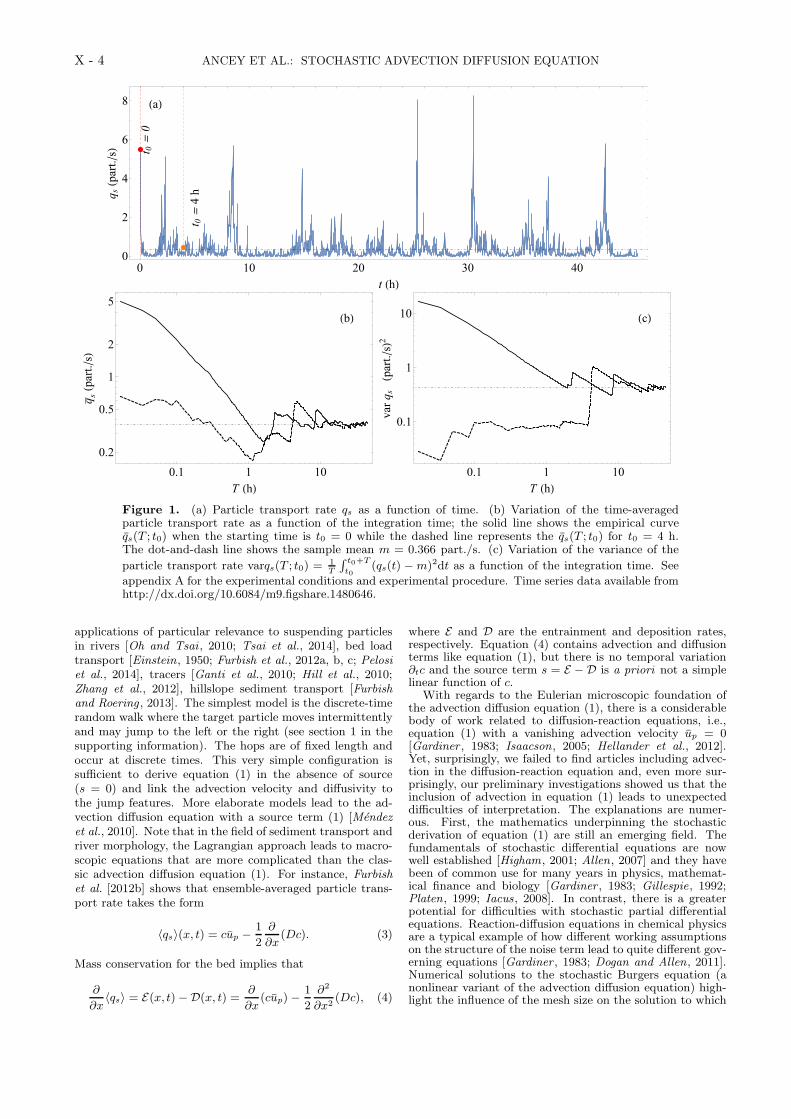
Sediment transport exhibits considerable spatial and tem-poral fluctuations. A typical example of this variability isgiven by Figure 1, which shows the time variation in thesediment transport rate for a gravel-bed flume experimentunder steady state conditions (see appendix A for furtherinformation on the experimental conditions). The resultingtime series illustrates various features of sediment transportat low transport rates: while the experiment was run for a

ANCEY ET AL.: STOCHASTIC ADVECTION DIFFUSION EQUATION X - 3

very long time (more than 50 h), the system did not reacha steady state characterized by gentle fluctuations around afixed value, but seemed to jump from states marked by lowsediment transport activity (possibly with transport ratesdropping to zero) to phases of intense sediment transport(with transport rates as large as 20 times the feeding rate).The bursts are likely to reflect the migration of bed forms(here anti-dunes) [Gomez , 1991].

For systems of this kind, fluctuations are likely to playan important part in the overall dynamics. Understandingthe part played by fluctuations in sediment transport is keyto various issues such as measurement of bedload transportrates and development of realistic morphodynamic models.We will outline these two problems below.

For a very long time, the effect of fluctuations on the mea-surement of transport rates has gone unnoticed. In recentdecades, with the development of high resolution techniquesfor measuring transport rates both in the laboratory andfield, it has been shown that the results depend a great dealon sampling time [Cudden and Hoey , 2003; Bunte and Abt ,2005; Singh et al., 2009; Campagnol et al., 2012; Gaeumanet al., 2015]. Closely related is the question of the optimumsampling time for a given setting, a problem that has as yetfew solutions. Figure 1b shows the time-averaged transportrate for the time series qs(t) shown in Figure 1a

qs(T ; t0) =1

T

∫ t0+T

t0

qs(t)dt, (2)

with T the sampling time and t0 the starting time. Forthis experiment, the time-averaged transport rate convergedvery slowly to the mean sample m: T must be as long as 2h for qs to come close to m to within ±20%. Even for verylong times (2 < T < 15 h), qs can deviate markedly fromthe mean sample as a result of bed form migration (the twopeaks of qs at T = 2 h and 9 h were associated with bedform development). Similar conclusions can be drawn forthe time-averaged variance, which slowly converges to thesample variance (see Figure 1c). Figure 1 also shows thatthe empirical curve qs(T ) depends a great deal on the start-ing time. If we start integrating qs when sediment transportis intense (e.g., t0 = 0 in Figure 1), the time-averaged sed-iment transport rate deviates initially by a factor 10 fromthe sample mean m. It comes as no surprise that if we se-lect the starting time (e.g., t0 = 4 h in Figure 1) so thatsediment transport is initially low, then the time-averagedsediment transport rate qs deviates less markedly from m.This example also demonstrates that the question of the op-timal sampling time for evaluating sediment transport ratehas no clear-cut answer.

This particular example shows that in contrast with manyfluctuating processes, the mean transport rate cannot be es-timated by merely smoothing the measurements over a shorttime span. It can require long sampling times even understeady state conditions (especially at low sediment trans-port rates) and so the question arises as to how to deter-mine proper estimates of qs under time-dependent flow con-ditions, e.g., when the timescale of water discharge changesis shorter than the optimum sampling time of qs.

The effect of sampling time on transport rate measure-ment is becoming even more apparent with field data. Reck-ing et al. [2012] tested different bed load transport equationsagainst instantaneous field measurements, volume accumu-lated at the event scale, volume accumulated at the annualand interannual scales, and time-integrated flume measure-ments. At the shortest timescales (say, a few minutes), allof the bed load equations tested failed to predict the meansediment transport rate to within one order of magnitude.The results were especially poor for coarse-bed rivers andsteep slopes. In contrast, on much longer timescales (say,one year), the predictions more closely matched the field

data, with relative errors (defined as the computed to mea-sured sediment volume ratio) lower than five in most cases.

Existing morphodynamic models are based on equationssuch as the advection diffusion equation (1). More elaboratemodels are composed of a set of governing equations. Forinstance, the Saint-Venant-Exner equations consist of massand momentum balance equations for the water stream andbed, and they are supplemented by closure equations forestimating flow resistance and sediment transport [Garcıa,2007]. In all of these models, the flow variables are smooth(or piecewise continuous) fields. In other words, these mod-els do not provide instantaneous values, but spatially or tem-porally averaged values. The effects of random perturba-tions on the mean flow are either ignored or incorporated inthe form of a diffusive term (the equivalent of the eddy dif-fusion process in turbulence models). Owing to the randomnature of sediment transport rates, morphodynamic modelsare fraught with difficulties of different order.

The first impediment has been highlighted by Figure 1.Any direct comparison between theory and observation ismade quite difficult because of the great sensitivity of themean sediment transport rate to sampling time. In practice,this hurdle has mostly been avoided by looking at globalpatterns such as the determination of the areas prone toaggradation/degradation or the evaluation of the sedimentbudget over a long characteristic time [e.g., see Ferguson andChurch, 2009].

Another difficulty arises when solving morphodynamicmodels numerically. Finite-volume methods are preferen-tially used for several reasons. First of all, discretizationbased on finite volumes is seen as more physical as theresulting discretized equations are obtained by integratingthe governing equations over elementary volumes of con-trol, expressing the flux (e.g., mass and momentum) throughthe boundaries of each volume, and updating the volume-averaged quantities [LeVeque, 2002; Toro, 2001]. A clearadvantage of this computational strategy is the possibilityto deal with discontinuities (e.g., a hydraulic jump). Asthe method makes use of volume averaging, it suffers frommesh size dependence when applied to random fields in thesame way as the time-averaged sediment transport rate (2)depends on sampling time. This subtle point will be illus-trated in the following; the reader is also referred to ourcompanion paper for further discussion on this point [Bo-horquez and Ancey , 2015].

1.2. Existing approaches to deriving the advection

diffusion equation

Equation (1) is often derived using conservation princi-ples of continuum mechanics and phenomenological laws.Arguments of this sort have been used to derive an advec-tion equation for particle activity [Charru, 2006; Lajeunesseet al., 2010]. The main shortcoming of this approach is thatit ignores or downplays the fluctuations of particle activityand its crucial influence on the sediment transport dynam-ics.

There is a considerable literature on the microscopic foun-dation of the advection diffusion equation and much of thisliterature makes use of the Lagrangian approach to deriveequation (1) [Mendez et al., 2010; Gillespie and Seitaridou,2013] with consideration for fluctuations of particle motion.Essentially, in this approach, a target particle is tracked.On the microscale, the erratic and intermittent motion ofthis particle can be described using random-walk models.Lagrangian models include a wide variety of processes de-pending on the working assumptions: the particle motioncan be seen as a series of jumps of fixed or random lengthoccurring at fixed or random times [Metzler and Klafter ,2000; Schumer et al., 2009]. The Lagrangian approach has


Figure 1. (a) Particle transport rate qs as a function of time. (b) Variation of the time-averagedparticle transport rate as a function of the integration time; the solid line shows the empirical curveqs(T ; t0) when the starting time is t0 = 0 while the dashed line represents the qs(T ; t0) for t0 = 4 h.The dot-and-dash line shows the sample mean m = 0.366 part./s. (c) Variation of the variance of the

particle transport rate varqs(T ; t0) =1

T

∫ t0+T

t0(qs(t) − m)2dt as a function of the integration time. See

appendix A for the experimental conditions and experimental procedure. Time series data available fromhttp://dx.doi.org/10.6084/m9.figshare.1480646.

applications of particular relevance to suspending particlesin rivers [Oh and Tsai , 2010; Tsai et al., 2014], bed loadtransport [Einstein, 1950; Furbish et al., 2012a, b, c; Pelosiet al., 2014], tracers [Ganti et al., 2010; Hill et al., 2010;Zhang et al., 2012], hillslope sediment transport [Furbishand Roering , 2013]. The simplest model is the discrete-timerandom walk where the target particle moves intermittentlyand may jump to the left or the right (see section 1 in thesupporting information). The hops are of fixed length andoccur at discrete times. This very simple configuration issufficient to derive equation (1) in the absence of source(s = 0) and link the advection velocity and diffusivity tothe jump features. More elaborate models lead to the ad-vection diffusion equation with a source term (1) [Mendez

et al., 2010]. Note that in the field of sediment transport andriver morphology, the Lagrangian approach leads to macro-scopic equations that are more complicated than the clas-sic advection diffusion equation (1). For instance, Furbishet al. [2012b] shows that ensemble-averaged particle trans-port rate takes the form

〈qs〉(x, t) = cup − 1

2

∂

∂x(Dc). (3)

Mass conservation for the bed implies that

∂

∂x〈qs〉 = E(x, t)−D(x, t) =

∂

∂x(cup)− 1

2

∂2

∂x2(Dc), (4)

where E and D are the entrainment and deposition rates,respectively. Equation (4) contains advection and diffusionterms like equation (1), but there is no temporal variation∂tc and the source term s = E − D is a priori not a simplelinear function of c.

With regards to the Eulerian microscopic foundation ofthe advection diffusion equation (1), there is a considerablebody of work related to diffusion-reaction equations, i.e.,equation (1) with a vanishing advection velocity up = 0[Gardiner , 1983; Isaacson, 2005; Hellander et al., 2012].Yet, surprisingly, we failed to find articles including advec-tion in the diffusion-reaction equation and, even more sur-prisingly, our preliminary investigations showed us that theinclusion of advection in equation (1) leads to unexpecteddifficulties of interpretation. The explanations are numer-ous. First, the mathematics underpinning the stochasticderivation of equation (1) are still an emerging field. Thefundamentals of stochastic differential equations are nowwell established [Higham, 2001; Allen, 2007] and they havebeen of common use for many years in physics, mathemat-ical finance and biology [Gardiner , 1983; Gillespie, 1992;Platen, 1999; Iacus, 2008]. In contrast, there is a greaterpotential for difficulties with stochastic partial differentialequations. Reaction-diffusion equations in chemical physicsare a typical example of how different working assumptionson the structure of the noise term lead to quite different gov-erning equations [Gardiner , 1983; Dogan and Allen, 2011].Numerical solutions to the stochastic Burgers equation (anonlinear variant of the advection diffusion equation) high-light the influence of the mesh size on the solution to which


the numerical schemes converge, a situation that contrastswith the deterministic case [Hairer and Voss, 2011]. Theinterpretation of white noise (Ito’s versus Stratonovich con-vention) relies on a working assumption that may also leadto conceptual and mathematical difficulties depending onthe rule chosen [Ridolfi et al., 2011] (see also section 2.3).

2. Markovian Eulerian Framework

Before tackling the question of the stochastic foundationof the advection diffusion (1) (see section 2.3), we summarizeour approach presented in earlier papers [Ancey et al., 2008;Ancey and Heyman, 2014]. A convenient framework for theinvestigation of the statistical properties of sediment trans-port is the theory of birth-death Markov processes, whichhas been quite successful in various fields such as popula-tion dynamics, epidemiology and chemical kinetics [Cox andMiller , 1965; Gillespie, 1992]. We think that it can also bea very powerful tool to better understand the dynamics ofsediment transport.

2.1. Outline of the Approach

We are interested in studying the variation in the par-ticle activity c(x, t) along a river. For the sake of simplic-ity, we consider a one-dimensional stream and ignore anycross-stream variation. On the microscopic scale, the parti-cle activity is linked to the number of moving particles Ncontained in a (control) volume of length ∆x. The idea un-derpinning the Markovian Eulerian framework is a generaland rather intuitive one, which consists in monitoring thechanges in the number moving particles over a time interval∆t within this control volume. This number N can varybecause particles can be entrained from the bed, depositedon the bed, enter the volume or leave it. These events occurrandomly and a priori independently and so, N is a discreterandom variable described by a probability P (n, t) of observ-ing N = n particles within the volume at time t. We studya subclass of Markov processes called birth-death processes,for which the number of particles can only experience jumpsof +1 or −1, which means in practice that the time inter-val ∆t must be short enough to allow the detection of suchjumps. Sediment transport is assumed to be sufficiently lowfor events to be distinguishable. At higher sediment trans-port rates, multiple events (erosion, deposition, emigration,and immigration) can occur within infinitesimal times, mak-ing the present stochastic framework irrelevant.

Our approach is Eulerian in that we do not track particlesindividually, but merely count the number of particles in acontrol volume. It is Markovian because we assume that thevariations in N in the time interval t and t+∆t depend pri-marily on ∆t. Said differently, we do not need the completehistory of N up to time t to determine what may happenin the time interval t and t + ∆t. It is discrete because weconsider a collection of finite-size particles within a controlvolume of finite length ∆x.

In this section, our goal is to determine the governingequation of N(t) as a function of the volume length ∆xand time step ∆t, then to derive a differential (macroscopic)equation for particle activity in the continuum limit (i.e., asthe parameters ∆x and ∆t approach zero).

2.2. Mass Balance and Governing Equation at the

Particle Scale

We split the one-dimensional stream into an array of Mcells i of length ∆x and we monitor the number of movingparticles Ni in each cell (see Figure 2). More specifically,we are interested in calculating P (n; t) = Prob(N = n; t)the probability of observing n = (n1, · · · , nM ) particles in

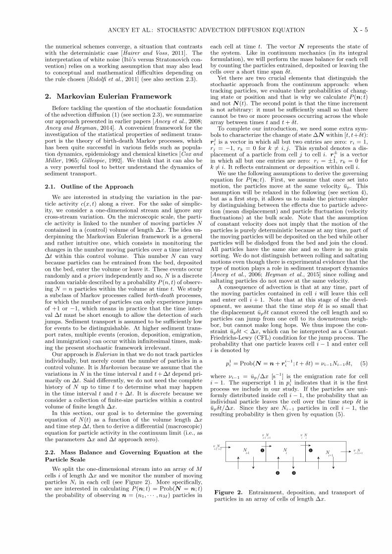
each cell at time t. The vector N represents the state ofthe system. Like in continuum mechanics (in its integralformulation), we will perform the mass balance for each cellby counting the particles entrained, deposited or leaving thecells over a short time span δt.

Yet there are two crucial elements that distinguish thestochastic approach from the continuum approach: whentracking particles, we evaluate their probabilities of chang-ing state or position and that is why we calculate P (n; t)and not N(t). The second point is that the time incrementis not arbitrary: it must be sufficiently small so that therecannot be two or more processes occurring across the wholearray between times t and t+ δt.

To complete our introduction, we need some extra sym-bols to characterize the change of state ∆N within [t, t+δt):rji is a vector in which all but two entries are zero: ri = 1,

rj = −1, rk = 0 for k 6= i, j. This symbol denotes a dis-placement of a particle from cell j to cell i. r

±i is a vector

in which all but one entries are zero: ri = ±1, rk = 0 fork 6= i. It reflects entrainment or deposition within cell i.

We use the following assumptions to derive the governingequation for P (n; t). First, we assume that once set intomotion, the particles move at the same velocity up. Thisassumption will be relaxed in the following (see section 4),but as a first step, it allows us to make the picture simplerby distinguishing between the effects due to particle advec-tion (mean displacement) and particle fluctuation (velocityfluctuations) at the bulk scale. Note that the assumptionof constant velocity does not imply that the motion of theparticles is purely deterministic because at any time, part ofthe moving particles will be deposited on the bed while otherparticles will be dislodged from the bed and join the cloud.All particles have the same size and so there is no grainsorting. We do not distinguish between rolling and saltatingmotions even though there is experimental evidence that thetype of motion plays a role in sediment transport dynamics[Ancey et al., 2006; Heyman et al., 2015] since rolling andsaltating particles do not move at the same velocity.

A consequence of advection is that at any time, part ofthe moving particles contained in cell i will leave this celland enter cell i + 1. Note that at this stage of the devel-opment, we assume that the time step δt is so small thatthe displacement upδt cannot exceed the cell length and soparticles can jump from one cell to its downstream neigh-bor, but cannot make long hops. We thus impose the con-straint upδt < ∆x, which can be interpreted as a Courant-Friedrichs-Lewy (CFL) condition for the jump process. Theprobability that one particle leaves cell i − 1 and enter celli is denoted by

p1i = Prob(N = n+ ri−1i ; t+ δt) = νi−1Ni−1δt, (5)

where νi−1 = up/∆x [s−1] is the emigration rate for celli − 1. The superscript 1 in p1i indicates that it is the firstprocess we include in our study. If the particles are uni-formly distributed inside cell i − 1, the probability that anindividual particle leaves the cell over the time step δt isupδt/∆x. Since they are Ni−1 particles in cell i − 1, theresulting probability is then given by equation (5).

N NNi-1i+1

i

n Ni-2i-2

n Ni-1i-1

n Nii

n Ni+1i+1

❶

❷ ❸

❶

Figure 2. Entrainment, deposition, and transport ofparticles in an array of cells of length ∆x.


Particles can be entrained and deposited. We assumethat the entrainment and deposition rates, E [part. s−1] andD [part. s−1] respectively, can be expanded as a power seriesof N

E = E0 + E1N + · · · , (6)

D = D0 +D1N + · · · . (7)

As we investigate linear models, the expansions are limitedto order 1. Concerning deposition, as there are N movingparticles, the deposition rate is necessarily linearly depen-dent on N and so D0 = 0. To keep the notation consistentwith our earlier papers [Ancey et al., 2008; Ancey and Hey-man, 2014], we denote D1 by σ [s−1]; we index it by i torecall that σ depends on position. The probability of depo-sition in cell i is then

p2i = Prob(N = n+ r−i ; t+ δt) = σiNiδt. (8)

For entrainment, we interpret E0 as the effect of the waterstream alone on the bed. Moving particles induce perturba-tions, collisions, changes in the water turbulence, etc., whichcan also lead to dislodge particles from the bed. We refer tothe coefficient E1 as collective entrainment, but this name isconfusing to some degree as it may lead to think that sev-eral particles are simultaneously entrained. This is not themeaning here (massive entrainment would conflict with ourworking assumption that there is no more than one eventover the time span δt). Again, for consistency with our ear-lier publications [Ancey et al., 2008; Ancey and Heyman,2014], we denote E0 and E1 by λ [part. s−1] and µ [s−1]. Theprobability of entrainment in cell i is thus

p3i = Prob(N = n+ r+i ; t+ δt) = (λi + µiNi)δt. (9)

In equations (5), (8), and (2), we have calculated thetransition probabilities pki (k = 1, 2, and 3) that process koccurs in cell i (1 ≤ i ≤ M). We can now calculate theprobability of change for the whole system. We will not re-produce the derivation of the governing equation, which canbe found in our earlier papers [Ancey et al., 2008; Ancey andHeyman, 2014]. The fundamental idea is that starting fromthe Chapman-Kolmogorov equation

P (n, t+ δt) =∑

∆n,k=1,2,3

P (n+∆n, t)pk(n+∆n → n, δt)

(10)and taking the limit δt → 0, we end up with the forwardKolmogorov equation (also called the master equation)

∂P

∂t(n; t) =

M∑

i=1

(ni + 1)(P (n+ rii+1, t)νi (11)

+P (n+ r+i , t)σi)

+P (n+ r−i , t)(λi + µi(ni − 1))

+P (n+ ri−1i , t)νi−1ni−1

−P (n, t)(νi−1ni−1 + λi + µini+1 + νini + σini),

which is the governing equation for N .Apart from the one-cell case (M = 1) [Ancey et al., 2008],

there is no technique for solving this equation analytically.In this respect, the governing equation (11) for N does notallow us to directly derive a macroscopic equation for N inthe form of an advection diffusion equation. However, var-ious techniques can be used for finding numerical solutionsand analytical approximations, and for transforming the for-ward Kolmogorov equation (11) into a more tractable form(see sections 2 and 3 in the supporting information). In the

following, we will use an exact technique (the Poisson rep-resentation) to transform the forward Kolmogorov equation(11) to gain analytical traction. Direct numerical solutionsof the forward Kolmogorov equation (11) are also possible[Gillespie, 1992, 2001; Lipshtat , 2007; Pineda-Krch, 2008].

2.3. Derivation of the Ensemble-Averaged Equation

for Particle Activity c

To proceed with the determination of solutions to equa-tion (11), we use an elegant and exact technique, which canbe thought of as a Laplace-like transform: the Poisson rep-resentation makes it possible to pass from the discrete ran-dom variable N to the (dimensionless) continuous randomvariable a (here called the Poisson rate) [Gardiner , 1983]

P (n, t) =∏

i

∫

R+

e−aiani

n!f(a, t)da, (12)

where a = (ai) ≥ 0 for i = 1, 2, . . . and f(a, t) is the multi-variate probability density function of a. Instead of workingwith the discrete random variable N , we now work with thecontinuous random variable a = (a1, a2, . . .). It is oftenmore convenient to work in another functional space to sim-plify the equations (like Fourier and Laplace transforms),but the way back to the original space may be impossible.Here, we will avoid this issue by using an interesting featureof the Poisson representation, which is the relationship be-tween the p-factorial moments of N and the p-moments ofa. In particular, we have

〈N〉 = 〈a〉 and varN = var a+ 〈a〉 (13)

which will be very useful in the following.Substituting the Poisson expansion (12) into the forward

Kolmogorov equation (11) and after a few algebraic manip-ulations (see section 3 in the supporting information), weend up with a governing equation for f(a, t)

∂

∂tf(a, t) =

∑

i

µi∂2aif

∂a2i

(14)

− ∂

∂ai{[λi − ai(σi + νi − µi)] f}

+∂

∂ai−1

(νi−1ai−1f).

The main advantages of this transformation appear hereclearly: we have reduced the degree of coupling betweenthe equations and the resulting set of equations is a multi-variate advection diffusion equation that can be interpretedas a Fokker-Planck equation. Therefore, we can use theequivalence between Fokker-Planck equations and stochas-tic differential (Langevin) equations [Gardiner , 1983]. TheLangevin representation equivalent to equation (14) is

dai(t) = (λi − ai(σi − µi) + νi−1ai−1 − νiai) dt+√

2µiaidWi(t),(15)

which holds for ai ≥ 0 (i = 2, 3 . . .) and where Wi [s1/2] is a

Wiener process (white noise) for cell i. Under homogeneousconditions (λi = λ, σi = σ and µi = µ for 1 ≤ i ≤ M), themean steady-state solution to the Langevin equation (15) is

〈a〉ss =λ

σ − µ. (16)

It is now very tempting to take the continuum limit∆x → 0 and introduce the Poisson density b [m−1], par-ticle activity γ [m], and ensemble-averaged particle activity


Table 1. Correspondence between the variables used.

Real world Poisson space

discrete random variable NPoisson transform−−−−−−−−−−−−→ a

number of moving particles Poisson rate

continuous random variable γ = lim∆x→0

N

∆xb = lim

∆x→0

a

∆xparticle activity Poisson density

ensemble-averaged variable c = 〈γ〉mean particle activity

c [m]:

b(xi, t) = lim∆x→0

ai(t)

∆x, (17)

γ(xi, t) = lim∆x→0

pNi(t)

B∆xand c(xi, t) = 〈γ〉,

with xi the center of cell i, B [m] the stream width, andp [m3] the particle volume. Table 1 recaps the differentvariables used and their correspondence.

If ai were a continuous variable, it would be also verytempting to interpret the difference νi−1ai−1 − νiai as thegradient −∂x(upb) in the the continuum limit ∆x → 0. Ifso, we should end up with a governing equation for b

∂

∂tb(x, t) +

∂

∂x(upb) = λ− (σ − µ)b+

√

2µbξb, (18)

where we introduce λ = λ/∆x [m−1 s−1] the entrainmentrate per unit length and we define a Gaussian noise termξb(x, t) [m−1/2 s−1/2] such that 〈ξb(x, t)ξb(x′, t′)〉 = δx(x −x′)δt(t− t′), i.e., a white noise term that is uncorrelated intime and space, and δx [m−1] and δt [s−1] are Kronecker’sdeltas (i.e., δt(t) = 0 if t 6= 0, and 1 for t = 0). Within ourframework, the white noise term ξb(x, t) is a generalizationof white noise, which satisfies

lim∆x→0

dWi(t)√∆x

= ξb(x, t)dt. (19)

This definition of ξb(x, t) is essential to properly encodingthe white noise term in the numerical simulations.

Making use of the relation (13) between the a- and n-moments and the rule 〈√2µbξb〉 = 0, we deduce that theensemble average of equation (18) leads to a simple advec-tion equation for the particle activity c

∂

∂tc(x, t) +

∂

∂x(upc) = s(c), (20)

where s(c) = λ′ − (σ − µ)c is the linear source term andλ′ = pλ/B [m s−1] is the volumetric entrainment rate. Acaveat is in order here: the treatment of the colored noiseterm

√2µbξb in equation (18) can be achieved following two

different approaches [Gardiner , 1983]: in the Ito interpreta-tion, the value of b is taken before the jump; an importantconsequence is that 〈√2µbξb〉 = 0. Another possibility isthe Stratonovich interpretation, which takes the mean of bbefore and after the jump (and in that case 〈√2µbξb〉 6= 0).The latter interpretation is often seen as the most naturalchoice from a physical standpoint [Ridolfi et al., 2011], butunfortunately it leads to substantial mathematical difficul-ties when trying to solve stochastic differential equations an-alytically. So, following the usage in the physics of reaction-diffusion problems [Gardiner , 1983], we have adopted theIto convention. Comparing equations (1) and (20), we notethat the advection terms are not strictly similar (except ifthe advection velocity does not depend on x): in the originaladvection diffusion equation (1), the operator ∂t + up∂x isthe material derivative and represents the rate of change ofparticle activity observed by particles. The advection dif-fusion equation (20) is in conservation and the advection

term ∂x(upc) represents the flux of particle activity througha vertical slice.

The statistical properties of c can be inferred from equa-tions (18) and (13). Under homogeneous steady state condi-tions, we find (see section 4 in the supporting information)for the mean Poisson density, the spatial cross correlation,and variance

〈b〉ss =λ

σ − µ, (21)

〈b(x)b(x+ r)〉ss = 〈b〉ssµδr(r) + λ

σ − µ,

and varss b =µλ

(σ − µ)2δr(0),

where δr(r) [m−1] is Kronecker’s delta, and for the autocor-

relation function

ρ(t) = exp(−(σ − µ)t). (22)

Surprisingly, these properties are independent of the advec-tion velocity up. This may seem a priori plausible in thatadvection is just a mode of transport of particles, which un-der steady state conditions fades out. Note also that theseproperties are independent of the position and so they holdtrue for any x or over any control volume. It also follows thatthe analytical results obtained for one-cell systems (M = 1)should hold true here, in particular the probability densityfunction of ai (under steady state conditions) should be thegamma distribution Ga(α, β) with parameters α = λ/µ andβ = µ/(σ − µ) [Ancey and Heyman, 2014].

However, as shown just below (see section 3), numericalsimulations of the Langevin equations (15) reveal that thestory is a bit more complicated. They demonstrate thatdiffusion-like effects occur and thus, the link between theadvection equation (20) (giving a picture of the system atthe bulk scale) and the underlying Langevin equations (15)(describing the system at the microscale) is more subtle thanwhat the derivation above suggests.

3. Numerical Tests

In the following, we will analyse the microscopic behaviorin particular cases by solving the system of Langevin equa-tions (15) and compare the results with the macroscopicfeatures predicted by the continuum formulation (20) or theexpected statistical properties (21).

We solved the system of Langevin equations (15) nu-merically using an Euler scheme with time step dt = 0.01s (see section 5 in the supporting information) [Higham,2001; Iacus, 2008]. The computational domain was splitinto M = 100 cells of length ∆x = 1 m. The sample meanand variance, 〈n〉 and vara for each cell were computed over500 simulations. Note that making use of equations (13)and (17), we also find the relationship between c and 〈N〉

〈c〉ss =p

B∆x〈N〉ss and varss a = ∆x2varss b, (23)

since the variance of b is found to be independent of x. Thecontinuum formulation (20) is a simple hyperbolic partial


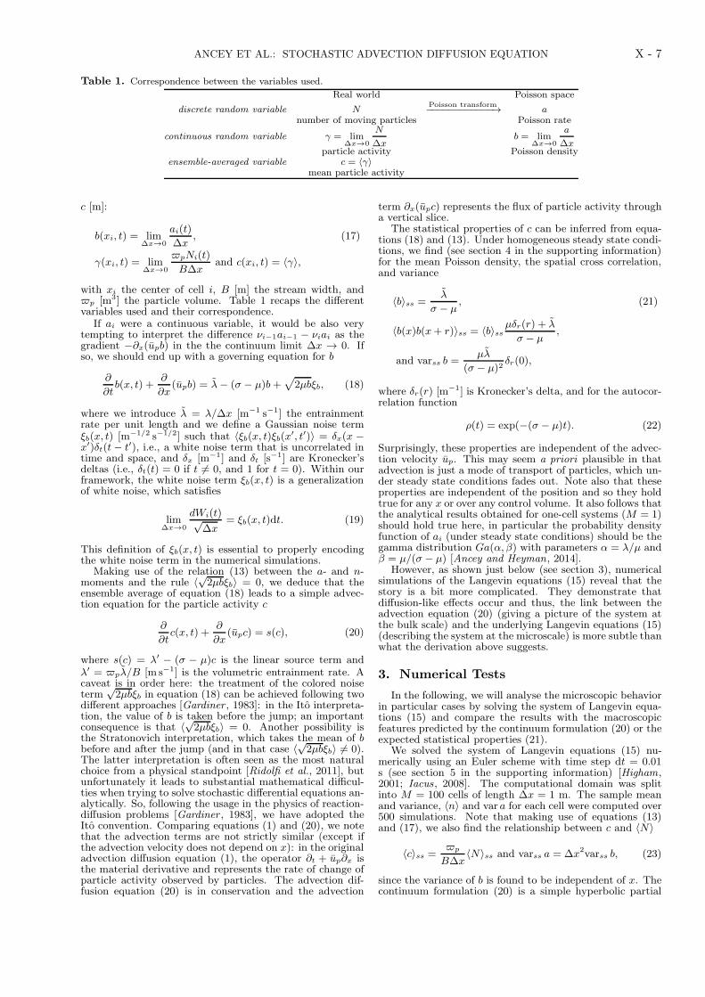
Figure 3. Example of simulation of the Langevin equa-tions (15) with λ = 2 s−1, σ = 5 s−1, µ = 4 s−1, ν = 5 s−1

(D∗ = 2.5 m s−2). The dots represents the mean parti-cle activity averaged over 500 samples obtained by solv-ing (15) numerically using an Euler scheme [Iacus, 2008]with a time step dt = 0.01 s. The dashed line shows thepure advection behavior (20) at times t = 0, 1, 2, 4, 8 s.The exact solution to equation (20) is provided in section11 of the supporting information. The initial (t = 0 s)conditions are shown in purple. The boundary conditionsare c = 0. We show only the first 25 cells.

differential equation that can be solved exactly using themethod of characteristics (see section 11 in the supportinginformation).

3.1. Mean Behavior of the Particle Activity

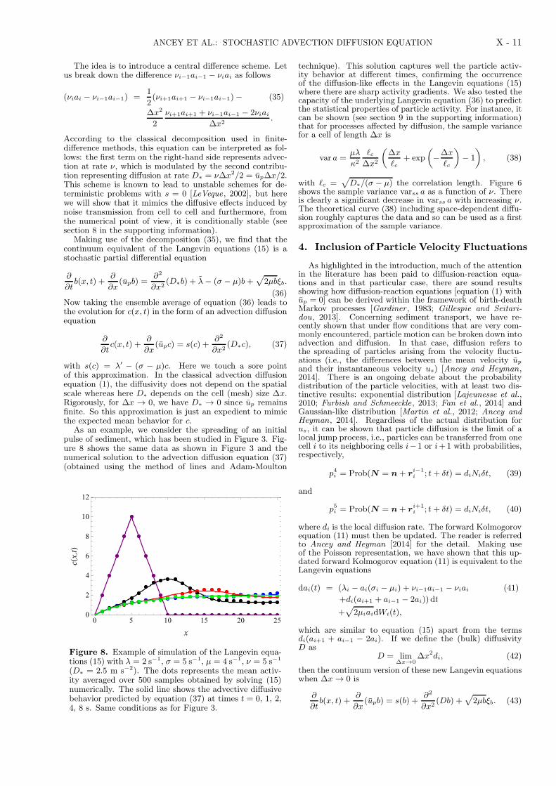
Let us first consider a sharp gradient in the particle activ-ity and let us see how this particle activity evolves with timewhen at the microscale, the particles are advected at con-stant velocity up. Figure 3 shows the propagation of an ini-tial pulse of sediment: the evolution of the initial (triangle-shaped) pulse is dictated by the displacement, deposition,and entrainment processes (5), (8), and (2). In the numeri-cal simulations (dots) at t = 1 s, the initial peak is rapidlysmoothed out while on the right, the particle activity tendscontinuously to a constant value. This contrasts with theadvection solution (dashed line), which conserves the initialshape, i.e., a peak and a sharp transition from the peak tothe plateau. This simple example shows that the advectionequation (20) captures the mean behavior fairly well, butit fails to provide the correct values in regions marked bya discontinuity in the particle activity gradient. This is anindication of nonlocal or diffusive effects, which smear outsharp variations in c.

3.2. Statistical Behavior of the Particle Activity

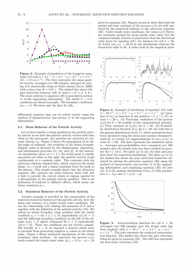
Another example is provided by the computation of theexpected statistical features of the particle activity, here themean and variance of a under steady state conditions. Weuse the relationship (13) relating the moments of N and atogether with the definition of the particle activity (18). Wesolved an initial boundary value problem with the initialcondition ai = 1 for 1 ≤ i ≤ M (equivalently c(x, 0) = 1)and the following boundary condition on the left of the do-main a0(t) = 0 (ghost cell)epend for t > 0 (equivalentlyc(0, t) = 0). These two conditions are not strictly compat-ible initially at x = 0; we imposed a nonzero initial stateto preclude from generating negative ai values in the initialsteps. Figure 4 shows numerical simulations of this initialboundary value problem. As expected, the process ai(t)tends toward the steady state value 〈a〉ss = λ/(σ − µ) = 10

given by equation (16): Figures 4a and 4c show that both thespatial and time variation of the process ai(t) are well cap-tured by the analytical solution to the advection equation(20). Under steady state conditions, the values ai(t) fluctu-ate randomly around the mean steady state value, but thecomputed sample variance is much lower than the theoreticalvalue given by equation (21): for instance for cell k = 50,we found varss ak = 23.19 in our simulations whereas thetheoretical value is 40. A closer look at the empirical prob-

Figure 4. Example of simulation of equation (15) withλ = 10 s−1, σ = 5 s−1, µ = 4 s−1, ν = 1 s−1. (a) varia-tion of 〈ai〉 as function of the position i (1 ≤ i ≤ M) attime t = 20 s. (b) Particular realization of the processak(t) for k = 50 (middle of the computational domain).(c) Time variation of 〈ak(t)〉 for k = 50. (d) Probabil-ity distribution function of ak for k = 50; the solid line isthe gamma distribution Ga(α, β), whose parameters havebeen calculated using the mean and variance obtained it-eratively in section 3.3 (approximation of varss a/〈a〉 toorder K = 20). The dots represents the simulated valuesai. Averages and probabilities were computed over 500samples once the steady state has been reached (in prac-tice for t ≥ 10 s). For plots (a) to (d), the dots and graylines show the numerical simulations. For plots (a) to (c)the dashed line shows the pure advection behaviour ob-tained by solving the advection equation (20) using themethod of characteristics (see section 11 of the support-ing information) and employing equation (23); for plot(d), it is the gamma distribution Ga(α, β) with parame-ters α = λ/µ and β = µ/(σ − µ).

Figure 5. Autocorrelation function for cell k = 50(averaged over 500 samples once the steady state hasbeen reached) with λ = 10 s−1, σ = 5 s−1, µ = 4 s−1,ν = 1 s−1. The dots represent the empirical autocorrela-tion function. The dashed line shows the pure advectionbehavior given by equation (22). The solid line representsthe first-order correction (34).


ability distribution (see Figure 4d) reveals that the theo-retical gamma distribution Ga(α, β) roughly describes theempirical probabilities. The difference is especially visiblein the tail of the distribution (for ak > 20), for which the-ory overestimates the probabilities significantly. Figure 5shows the empirical autocorrelation function and its the-oretical expression (22). Theory clearly overestimates theautocorrelation.

As a summary, we have found that the mean behavior isclosely described by the advection equation (20): the steadystate and the transient to this regime are fairly well de-scribed, but deviations from the simulated behavior are seenin regions characterized by sharp transitions in the particleactivity. Moreover, there is clear evidence that the theoreti-cal statistical properties (here, variance and autocorrelation)are poorly estimated by equation (21).

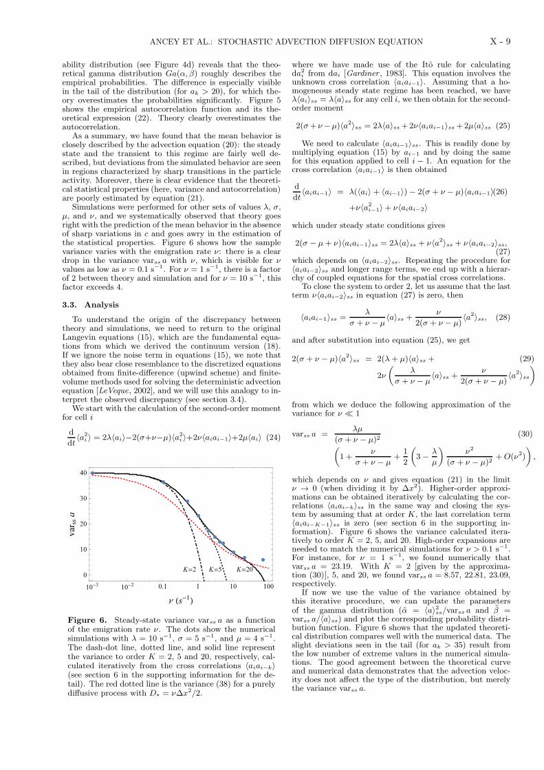
Simulations were performed for other sets of values λ, σ,µ, and ν, and we systematically observed that theory goesright with the prediction of the mean behavior in the absenceof sharp variations in c and goes awry in the estimation ofthe statistical properties. Figure 6 shows how the samplevariance varies with the emigration rate ν: there is a cleardrop in the variance varss a with ν, which is visible for νvalues as low as ν = 0.1 s−1. For ν = 1 s−1, there is a factorof 2 between theory and simulation and for ν = 10 s−1, thisfactor exceeds 4.

3.3. Analysis

To understand the origin of the discrepancy betweentheory and simulations, we need to return to the originalLangevin equations (15), which are the fundamental equa-tions from which we derived the continuum version (18).If we ignore the noise term in equations (15), we note thatthey also bear close resemblance to the discretized equationsobtained from finite-difference (upwind scheme) and finite-volume methods used for solving the deterministic advectionequation [LeVeque, 2002], and we will use this analogy to in-terpret the observed discrepancy (see section 3.4).

We start with the calculation of the second-order momentfor cell i

d

dt〈a2

i 〉 = 2λ〈ai〉−2(σ+ν−µ)〈a2i 〉+2ν〈aiai−1〉+2µ〈ai〉 (24)

Figure 6. Steady-state variance varss a as a functionof the emigration rate ν. The dots show the numericalsimulations with λ = 10 s−1, σ = 5 s−1, and µ = 4 s−1.The dash-dot line, dotted line, and solid line representthe variance to order K = 2, 5 and 20, respectively, cal-culated iteratively from the cross correlations 〈aiai−k〉(see section 6 in the supporting information for the de-tail). The red dotted line is the variance (38) for a purelydiffusive process with D∗ = ν∆x2/2.

where we have made use of the Ito rule for calculatingda2

i from dai [Gardiner , 1983]. This equation involves theunknown cross correlation 〈aiai−1〉. Assuming that a ho-mogeneous steady state regime has been reached, we haveλ〈ai〉ss = λ〈a〉ss for any cell i, we then obtain for the second-order moment

2(σ+ ν−µ)〈a2〉ss = 2λ〈a〉ss +2ν〈aiai−1〉ss +2µ〈a〉ss (25)

We need to calculate 〈aiai−1〉ss. This is readily done bymultiplying equation (15) by ai−1 and by doing the samefor this equation applied to cell i − 1. An equation for thecross correlation 〈aiai−1〉 is then obtained

d

dt〈aiai−1〉 = λ(〈ai〉+ 〈ai−1〉)− 2(σ + ν − µ)〈aiai−1〉(26)

+ν〈a2i−1〉+ ν〈aiai−2〉

which under steady state conditions gives

2(σ − µ+ ν)〈aiai−1〉ss = 2λ〈a〉ss + ν〈a2〉ss + ν〈aiai−2〉ss,(27)

which depends on 〈aiai−2〉ss. Repeating the procedure for〈aiai−2〉ss and longer range terms, we end up with a hierar-chy of coupled equations for the spatial cross correlations.

To close the system to order 2, let us assume that the lastterm ν〈aiai−2〉ss in equation (27) is zero, then

〈aiai−1〉ss =λ

σ + ν − µ〈a〉ss + ν

2(σ + ν − µ)〈a2〉ss, (28)

and after substitution into equation (25), we get

2(σ + ν − µ)〈a2〉ss = 2(λ+ µ)〈a〉ss + (29)

2ν

(

λ

σ + ν − µ〈a〉ss + ν

2(σ + ν − µ)〈a2〉ss

)

from which we deduce the following approximation of thevariance for ν ≪ 1

varss a =λµ

(σ + ν − µ)2(30)

(

1 +ν

σ + ν − µ+

1

2

(

3− λ

µ

)

ν2

(σ + ν − µ)2+O(ν2)

)

,

which depends on ν and gives equation (21) in the limitν → 0 (when dividing it by ∆x2). Higher-order approxi-mations can be obtained iteratively by calculating the cor-relations 〈aiai−k〉ss in the same way and closing the sys-tem by assuming that at order K, the last correlation term〈aiai−K−1〉ss is zero (see section 6 in the supporting in-formation). Figure 6 shows the variance calculated itera-tively to order K = 2, 5, and 20. High-order expansions areneeded to match the numerical simulations for ν > 0.1 s−1.For instance, for ν = 1 s−1, we found numerically thatvarss a = 23.19. With K = 2 [given by the approxima-tion (30)], 5, and 20, we found varss a = 8.57, 22.81, 23.09,respectively.

If now we use the value of the variance obtained bythis iterative procedure, we can update the parametersof the gamma distribution (α = 〈a〉2ss/varss a and β =varss a/〈a〉ss) and plot the corresponding probability distri-bution function. Figure 6 shows that the updated theoreti-cal distribution compares well with the numerical data. Theslight deviations seen in the tail (for ak > 35) result fromthe low number of extreme values in the numerical simula-tions. The good agreement between the theoretical curveand numerical data demonstrates that the advection veloc-ity does not affect the type of the distribution, but merelythe variance varss a.


The calculations show that in contrast with theoreticalpredictions, the variance of the simulated samples decreaseswith increasing ν because the cross correlation exhibits alonger range dependence than theory predicts. This intro-duces nonlocal effects, which take the appearance of diffu-sion. This is why the emigration rate ν affects the statisticalproperties of the particle activity in contrast with the theo-retical predictions (21).

In the sediment transport literature, the concept of nonlo-cal effects is used to describe situations in which the particleflux in a given place depends not only on local conditions,but also on hillslope conditions far upstream or downstreamof the point of measurement [Furbish and Roering , 2013].For models based on random walks, nonlocality is often as-sociated with large jumps of the particles (relative to thesize of the system) or correlation of velocities [Tucker andBradley , 2010]. Here, nonlocality arises because the spatialcross correlations are nonzero (see below) and the calcula-tion of the local variance (in cell i) requires the knowledgeof the spatial cross correlations over a significant distancefrom cell i (depending on the emigration rate ν) whereasfor a genuinely local advection process in a steady state,these spatial cross correlations should vanish. Another wayof looking at the issue of nonlocality is to express the meanPoisson rate 〈ai〉 as a convolution sum. Assuming that thesystem reaches a steady (but not necessarily homogeneous)state and taking the ensemble average of the Langevin equa-tions (15), we can recast the latter system of equations inmatrix form

A · 〈a〉 = Λ, (31)

where Λ is the column vector (λi)1≤i≤M and A is a M ×Mlower bidiagonal matrix, whose main diagonal elements areσi − µi + νi (1 ≤ i ≤ M) and the lower diagonal entriesare −νi−1 (1 ≤ i ≤ M − 1) (all other entries are zero). Theinverse of a lower bidiagonal matrix is a lower triangular ma-trix L, whose entries can be calculated exactly (see section12 in the supporting information). So we deduce that

〈a〉 = L ·Λ, (32)

or said differently, this means that the Poisson rate at cell idepends on what happens upstream of it

〈ai〉 =i

∑

k=1

Lijλj for 1 ≤ i ≤ M. (33)

Similar iterative calculations can be made with the auto-correlation function (see section 7 in the supporting infor-mation) and to leading order, we find

ρ(t) = exp(−(σ + ν − µ)t), (34)

which introduces a dependence on ν. Note that this auto-correlation function is the same as the one found in one-cell systems [Ancey et al., 2008]. Figure 5 compares theapproximate and empirical autocorrelation functions for νand shows a fairly good agreement between both, confirm-ing the effect of ν on the autocorrelation time: the higherthe emigration rate, the shorter the autocorrelation timetc = (σ + ν − µ)−1.

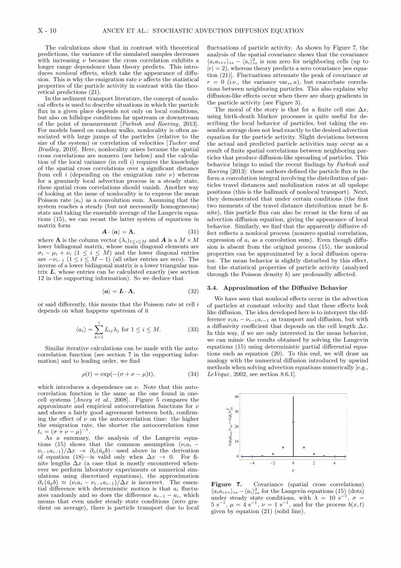
As a summary, the analysis of the Langevin equa-tions (15) shows that the common assumption (νiai −νi−1ai−1)/∆x → ∂x(upb)—used above in the derivationof equation (18)—is valid only when ∆x → 0. For fi-nite lengths ∆x (a case that is mostly encountered when-ever we perform laboratory experiments or numerical sim-ulations using discretized equations), the approximation∂x(upb) ≈ (νiai − νi−1ai−1)/∆x is incorrect. The essen-tial difference with deterministic motion is that ai fluctu-ates randomly and so does the difference ai−1 − ai, whichmeans that even under steady state conditions (zero gra-dient on average), there is particle transport due to local

fluctuations of particle activity. As shown by Figure 7, theanalysis of the spatial covariance shows that the covariance〈aiai+r〉ss − 〈ai〉2ss is non zero for neighboring cells (up to|r| = 2), whereas theory predicts a zero covariance [see equa-tion (21)]. Fluctuations attenuate the peak of covariance atr = 0 (i.e., the variance varss a), but exacerbate correla-tions between neighboring particles. This also explains whydiffusion-like effects occur when there are sharp gradients inthe particle activity (see Figure 3).

The moral of the story is that for a finite cell size ∆x,using birth-death Markov processes is quite useful for de-scribing the local behavior of particles, but taking the en-semble average does not lead exactly to the desired advectionequation for the particle activity. Slight deviations betweenthe actual and predicted particle activities may occur as aresult of finite spatial correlations between neighboring par-ticles that produce diffusion-like spreading of particles. Thisbehavior brings to mind the recent findings by Furbish andRoering [2013]: these authors defined the particle flux in theform a convolution integral involving the distribution of par-ticles travel distances and mobilization rates at all upslopepositions (this is the hallmark of nonlocal transport). Next,they demonstrated that under certain conditions (the firsttwo moments of the travel distance distribution must be fi-nite), this particle flux can also be recast in the form of anadvection diffusion equation, giving the appearance of localbehavior. Similarly, we find that the apparently diffusive ef-fect reflects a nonlocal process (nonzero spatial correlation,expression of ai as a convolution sum). Even though diffu-sion is absent from the original process (15), the nonlocalproperties can be approximated by a local diffusion opera-tor. The mean behavior is slightly disturbed by this effect,but the statistical properties of particle activity (analyzedthrough the Poisson density b) are profoundly affected.

3.4. Approximation of the Diffusive Behavior

We have seen that nonlocal effects occur in the advectionof particles at constant velocity and that these effects looklike diffusion. The idea developed here is to interpret the dif-ference νiai − νi−1ai−1 as transport and diffusion, but witha diffusivity coefficient that depends on the cell length ∆x.In this way, if we are only interested in the mean behavior,we can mimic the results obtained by solving the Langevinequations (15) using deterministic partial differential equa-tions such as equation (20). To this end, we will draw ananalogy with the numerical diffusion introduced by upwindmethods when solving advection equations numerically [e.g.,LeVeque, 2002, see section 8.6.1].

Figure 7. Covariance (spatial cross correlations)〈aiai+r〉ss−〈ai〉2ss for the Langevin equations (15) (dots)under steady state conditions, with λ = 10 s−1, σ =5 s−1, µ = 4 s−1, ν = 1 s−1, and for the process b(x, t)given by equation (21) (solid line).


The idea is to introduce a central difference scheme. Letus break down the difference νi−1ai−1 − νiai as follows

(νiai − νi−1ai−1) =1

2(νi+1ai+1 − νi−1ai−1)− (35)

∆x2

2

νi+1ai+1 + νi−1ai−1 − 2νiai

∆x2.

According to the classical decomposition used in finite-difference methods, this equation can be interpreted as fol-lows: the first term on the right-hand side represents advec-tion at rate ν, which is modulated by the second contribu-tion representing diffusion at rate D∗ = ν∆x2/2 = up∆x/2.This scheme is known to lead to unstable schemes for de-terministic problems with s = 0 [LeVeque, 2002], but herewe will show that it mimics the diffusive effects induced bynoise transmission from cell to cell and furthermore, fromthe numerical point of view, it is conditionally stable (seesection 8 in the supporting information).

Making use of the decomposition (35), we find that thecontinuum equivalent of the Langevin equations (15) is astochastic partial differential equation

∂

∂tb(x, t) +

∂

∂x(upb) =

∂2

∂x2(D∗b) + λ− (σ − µ)b+

√

2µbξb.

(36)Now taking the ensemble average of equation (36) leads tothe evolution for c(x, t) in the form of an advection diffusionequation

∂

∂tc(x, t) +

∂

∂x(upc) = s(c) +

∂2

∂x2(D∗c), (37)

with s(c) = λ′ − (σ − µ)c. Here we touch a sore pointof this approximation. In the classical advection diffusionequation (1), the diffusivity does not depend on the spatialscale whereas here D∗ depends on the cell (mesh) size ∆x.Rigorously, for ∆x → 0, we have D∗ → 0 since up remainsfinite. So this approximation is just an expedient to mimicthe expected mean behavior for c.

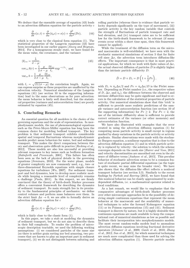
As an example, we consider the spreading of an initialpulse of sediment, which has been studied in Figure 3. Fig-ure 8 shows the same data as shown in Figure 3 and thenumerical solution to the advection diffusion equation (37)(obtained using the method of lines and Adam-Moulton

Figure 8. Example of simulation of the Langevin equa-tions (15) with λ = 2 s−1, σ = 5 s−1, µ = 4 s−1, ν = 5 s−1

(D∗ = 2.5 m s−2). The dots represents the mean activ-ity averaged over 500 samples obtained by solving (15)numerically. The solid line shows the advective diffusivebehavior predicted by equation (37) at times t = 0, 1, 2,4, 8 s. Same conditions as for Figure 3.

technique). This solution captures well the particle activ-ity behavior at different times, confirming the occurrenceof the diffusion-like effects in the Langevin equations (15)where there are sharp activity gradients. We also tested thecapacity of the underlying Langevin equation (36) to predictthe statistical properties of particle activity. For instance, itcan be shown (see section 9 in the supporting information)that for processes affected by diffusion, the sample variancefor a cell of length ∆x is

var a =µλ

κ2

ℓc∆x2

(

∆x

ℓc+ exp

(

−∆x

ℓc

)

− 1

)

, (38)

with ℓc =√

D∗/(σ − µ) the correlation length. Figure 6shows the sample variance varss a as a function of ν. Thereis clearly a significant decrease in varss a with increasing ν.The theoretical curve (38) including space-dependent diffu-sion roughly captures the data and so can be used as a firstapproximation of the sample variance.

4. Inclusion of Particle Velocity Fluctuations

As highlighted in the introduction, much of the attentionin the literature has been paid to diffusion-reaction equa-tions and in that particular case, there are sound resultsshowing how diffusion-reaction equations [equation (1) withup = 0] can be derived within the framework of birth-deathMarkov processes [Gardiner , 1983; Gillespie and Seitari-dou, 2013]. Concerning sediment transport, we have re-cently shown that under flow conditions that are very com-monly encountered, particle motion can be broken down intoadvection and diffusion. In that case, diffusion refers tothe spreading of particles arising from the velocity fluctu-ations (i.e., the differences between the mean velocity up

and their instantaneous velocity us) [Ancey and Heyman,2014]. There is an ongoing debate about the probabilitydistribution of the particle velocities, with at least two dis-tinctive results: exponential distribution [Lajeunesse et al.,2010; Furbish and Schmeeckle, 2013; Fan et al., 2014] andGaussian-like distribution [Martin et al., 2012; Ancey andHeyman, 2014]. Regardless of the actual distribution forus, it can be shown that particle diffusion is the limit of alocal jump process, i.e., particles can be transferred from onecell i to its neighboring cells i−1 or i+1 with probabilities,respectively,

p4i = Prob(N = n+ ri−1i ; t+ δt) = diNiδt, (39)

and

p5i = Prob(N = n+ ri+1i ; t+ δt) = diNiδt, (40)

where di is the local diffusion rate. The forward Kolmogorovequation (11) must then be updated. The reader is referredto Ancey and Heyman [2014] for the detail. Making useof the Poisson representation, we have shown that this up-dated forward Kolmogorov equation (11) is equivalent to theLangevin equations

dai(t) = (λi − ai(σi − µi) + νi−1ai−1 − νiai (41)

+di(ai+1 + ai−1 − 2ai)) dt

+√

2µiaidWi(t),

which are similar to equation (15) apart from the termsdi(ai+1 + ai−1 − 2ai). If we define the (bulk) diffusivityD as

D = lim∆x→0

∆x2di, (42)

then the continuum version of these new Langevin equationswhen ∆x → 0 is

∂

∂tb(x, t) +

∂

∂x(upb) = s(b) +

∂2

∂x2(Db) +

√

2µbξb. (43)


We deduce that the ensemble average of equation (43) leadsto an advection diffusion equation for the particle activity c

∂

∂tc(x, t) +

∂

∂x(upc) = s(c) +

∂2

∂x2(Dc), (44)

which is very close to the classical form equation (1). Thestatistical properties of the Langevin equations (43) havebeen investigated in our earlier papers [Ancey and Heyman,2014]. For a homogeneous steady state, we have found forthe mean value, the covariance, and the variance

〈b〉ss =λ

σ − µ, (45)

covss b(r) =1

2

µ

σ − µ

〈b〉ssℓc

exp−r/ℓc , and

varss b =1

2

µ

σ − µ

〈b〉ssℓc

,

with ℓc =√

D/(σ − µ) the correlation length. Again, wecan express surprise as these properties are unaffected by theadvection velocity. Numerical simulations of the Langevinequations (41) (see section 10 in the supporting informa-tion) lead to the same observations as for pure advection:the mean behavior is fairly well described, but the statisti-cal properties (variance and autocorrelation time) are poorlyestimated by equation (45).

5. Concluding Remarks

An essential question for all modelers is the choice of thegoverning equations and the scale of representation. In mor-phodynamic models, the use of phenomenological equationssuch as the Peter-Meyer-Muller equation has long been thecommon choice for modeling bedload transport. The keyproblem is that sediment transport exhibits considerablespatial and temporal fluctuations whereas morphodynamicmodels predict mean behaviors for water, bed and sedimenttransport. This makes the direct comparison between the-ory and observation quite difficult in practice [Recking et al.,2012]. These models are also less successful at providingrelevant responses to key issues such as bedform formation[Balmforth and Provenzale, 2001]. This failure has oftenbeen seen as the lack of physical details in the governingequations [Seminara, 2010]. For the water phase, modelsof greater complexity are now commonly used, e.g., two- orthree-dimensional Reynolds equations with simple closureequations for turbulence [Wu, 2007]. For sediment trans-port and bed dynamics, how to develop more realistic mod-els while keeping a reasonable level of complexity remainsa challenge [Paola, 2011]. In this respect, we are firmlyconvinced that the theory of birth-death Markov processesoffers a convenient framework for describing the dynamicsof sediment transport. Its main strength lies in its proxim-ity to the fundamental principles of mechanics: we definecontrol volumes and perform mass balances over them. Inthe strict limit ∆x → 0, we are able to formally derive anadvection diffusion equation for c

∂

∂tc(x, t) +

∂

∂x(upc) = s(c) +

∂2

∂x2(Dc),

which is fairly close to the classic form (1).In this paper, we take a stab at modeling the dynamics

of sediment transport, but we do not aim to describe themin their full complexity. To render the problem of micro-scopic description tractable, we used the following workingassumptions: (i) we considered particles of the same size(so there is neither grain sorting nor bed armoring, two pro-cesses that are known to play an important part in sedimenttransport), (ii) we do not distinguish between saltating and

rolling particles (whereas there is evidence that particle ve-locity depends significantly on the type of movement), (iii)particle activity is the key random variable that controlsthe strength of fluctuations of particle transport rate andbed elevation, and (iv) transport rates are to be sufficientlow for the birth-death framework to be relevant (if manyevents occur within a short time span, then this frameworkcannot be applied).

While the treatment of the diffusion term on the micro-and macroscales is well-established, we have seen with thestochastic numerical simulations of section 3 that for finitecell sizes ∆x, the advection term introduces diffusion-likeeffects. The important consequence is that in most practi-cal applications, for which we work with finite values of ∆x,the actual observed diffusion of particles D is slightly higherthan the intrinsic particle diffusivity D:

D = D +D∗ = D

(

1 +1

2Pe

)

, (46)

with D∗ ≈ up∆x/2 and Pe = up∆x/D is the Peclet num-ber. Depending on Peclet number (i.e., the respective valuesof D, ∆x, and up), the difference between the observed andintrinsic diffusivities may be quite significant and lead to er-rors in the calculation of the statistical properties of particleactivity. Our numerical simulations show that this ‘trick’ issufficient to provide more realistic predictions of the sam-ple variance and autocorrelation function (see section 10 ofthe supporting information) for Pe ≥ 2. For Pe < 2, theuse of the intrinsic diffusivity alone is sufficient to providecorrect estimates of the variance (or other moments) andautocorrelation function.

We have also illustrated with examples that the errorcreated in using the advection diffusion equation (1) forcomputing mean particle activity is small except in regionsmarked by sharp variations in the particle activity or activitygradients. Similar observations were made with the stochas-tic Burgers equation, a nonlinear equation that is close to theadvection diffusion equation (1) and in which particle activ-ity is replaced by velocity: the solution to which the schemeconverges depends on the mesh size [Hairer and Voss, 2011]and velocity discontinuities are smoothed out even in the ab-sence of diffusive terms [Audusse et al., 2015]. This peculiarbehavior of stochastic advection seems to be a common fea-ture of stochastic partial differential equations (as the topicis quite recent, we may miss the broader view). We havealso shown that the diffusion-like effect reflects a nonlocaltransport behavior (see section 3.3). Similarly to the recentfindings by Furbish and Roering [2013], we have found thatthis nonlocal behavior can be closely approximated by scale-dependent diffusion, i.e. a mathematical operator related tolocal conditions.

As a last remark, we would like to emphasize that thecomparative advantages of birth-death Markov processesover other microscopic approaches lie in the possibility of de-riving simple continuum equations that represent the meanbehavior at the macroscale and the availability of numer-ical techniques to solve the forward Kolmogorov equation(11) or its Poisson representations (15) and (41). Sedimenttransport is discrete by nature, but it is highly desirable thatcontinuum equations are made available to keep the compu-tational cost of numerical simulations as low as possible andfacilitate their incorporation into morphodynamics models.The most recent random-walks models lead to anomalousadvection diffusion equations involving fractional derivativeoperators [Schumer et al., 2009; Ganti et al., 2010; Zhanget al., 2012; Sun et al., 2015], for which numerical techniquesare much more complicated than those used for solving theadvection diffusion equation (1). Discrete particle models


and automaton models have attracted growing attention inrecent years [Narteau et al., 2009; Tucker and Bradley , 2010;Hodge and Hoey , 2012; Gabet and Mendoza, 2012]. Whiletheir numerical implementation is simple, there is no tech-nique for deriving continuum equations from the rules usedto describe the particles’ behavior in their environment.

Table of Notation

Here we provide the list of variables used in the paper,their meaning, physical units, and the reference to the equa-tions or sections, in which they were introduced.

Roman symbols

Variable Meaning

a, a Poisson rateai Poisson rate for cell i, equation (12)b Poisson density [m−1] equation (16)B flume width [m]c mean particle activity [m]D particle diffusivity [m s−2]di local diffusion rate [m−1 s−2], equation (36)D∗ fake diffusivity [m s−2], equation (40)D deposition rate per unit area [ s−1], equation (7)E entrainment rate per unit area [s−1], equation

(6)f probability density function in the a-spaceg gravity acceleration g = 9.81 m s−2

ℓc correlation length [m], equation (39)N number of moving particles within the window〈N〉 mean number of particles within the windowP probability density functionPe Peclet number Pe = up∆x/Dqs time-averaged particle sediment rate [part. s−1]qs instantaneous particle sediment rate [part. s−1]r position vector [m]t time [s]tc autocorrelation time [s]up mean particle (advection) velocity in [m s−1]

W Wiener process [s1/2]

Wi local Wiener process [s1/2], equation (15)x streamwise coordinate [m]

Greek and compound symbols

variable meaning

δr, δt, δx Kronecker’s delta ([m−1], [s−1], [m−1], respec-tively)

δt time increment [s]∆x space increment [m]γ particle activity (random variable) [m]κ difference κ = σ − µ [s−1]λ entrainment rate [s−1]

λ entrainment rate per unit length [m−1 s−1]λ′ volumetric entrainment rate [m s−1]µ collective entrainment rate [s−1]ν emigration rate [s−1]ρ autocorrelation functionρp particle density [kg m−3]σ deposition rate [s−1]p particle volume [m3]

ξ Gaussian noise increment [s−1/2]ξb space and time Gaussian noise increment

[m−1/2s−1/2]

Appendix A: Experimental conditions

The data presented in Figure 1 were presented in anearlier publication [Heyman et al., 2014]. The time se-ries data along with a Mathematica notebook for comput-ing the particle transport rate and visualizing the time se-ries can be obtained from the following data repositoryhttp://dx.doi.org/10.6084/m9.figshare.1480646. Further in-formation on the experimental facility can be found in twoPhD theses [Mettra, 2014; Heyman, 2014] (available fromhttp://http://library.epfl.ch/theses/).

The flume was 2.5 m long and 8 cm wide. The meanbedstream inclination θ was 7% (4.0◦), but the bed formsdeveloped so that mean bed slope varied between 6% and8.4% over time. The water flow depth was h = 1.37cm on average, leading to a depth-averaged water velocityu = 53 cm s−1. The sediment was made of gravel with meandiameter d50 = 6.25 mm (d30 = 6.0 mm and d50 = 6.8 mm)and density ρp = 2690 kgm−3. The flume was supplied withgravel at a constant feeding rate qs = 0.37 part. s−1 (about0.12 g s−1).

The resulting Shields number was Sh = ρwh sin θ/((ρp −ρ)d50) = 0.09 (ρw = 103 kg2 m−3 the water density), theFroude number Fr = u/

√gh = 1.44, the flow Reynolds

number Re = uWh/(W + 2h)/νw = 5400 (W = 8 cm thechannel width, νw = 10−6 m2 s−1 the kinematic viscosityof water), the boundary Reynolds number Re′ = u∗h/νw =605 (u∗ =

√gh sin θ the shear velocity). We deduce that

the flow is fully turbulent and supercritical. Additionalexperiments have shown that the critical Shields number(threshold for incipient motion) determined by visual in-spection should be slightly lower than 0.07 [Mettra, 2014].The Shields diagram gives an upper bound for the criti-cal Shields number Shc close to 0.06 [Buffington, 1999] forRe′ ≈ 600. If we take this value, the transport stage isT = Sh/Shc − 1 = 0.5 and so we are just above the thresh-old of incipient motion. Note that the relative submergenceh/d50 = 2.2 is low (very shallow flow).

Upon leaving the channel, each particle hits a metallicplate and the impact is recorded by a small accelerome-ter operated at 20,000 Hz and tied to the plate. A peak-over-threshold method is then applied to detect the timesof the consecutive particle impacts [Mettra, 2014]. If suf-ficient damping is provided to avoid spurious vibrations ofthe plate, this method ensures excellent time resolution inpassage detection. As the grain size distribution is narrow,little error is made when converting the number of parti-cles per unit time to a (volumetric) sediment transport rate.The same measurement system is used at the flume inlet tomeasure the incoming sediment transport rate.

Using the accelerometer, we record the arrival time ofparticles at the flume outlet. We count the number n(t) ofparticles hitting the plate at the outlet between times t andt + ∆t (with ∆t = 60 s the sampling time) and define thesediment transport rate as

qs(t) =n(t)

∆t. (A1)

The experiment was run for 50 h. As the experimentstarted with a flat bed, a near-equilibrium state regime wasobserved after a few hours (once the mean bedstream slopewas adjusted and bedforms developed). The raw data in-cluded 67,972 events. We decided to keep the last 60,000events. Said differently, the time series shown in Figure 1corresponds to data acquired for times t > 8.73 h after theexperiment started.

Acknowledgments. The work presented here was sup-ported by the Swiss National Science Foundation under grants


No. 200021-160083 (a project called “The Stochastic Torrent:stochastic model for bed load transport on steep slope”) and No.200021-105193/1 (a project called “Transient free-surface flowsof concentrated suspensions–Application to geophysical flows,”funded by an R’Equip grant). We are grateful to Prof. VaughanVoller and the associate editor for the numerous astute com-ments and helpful criticisms. Additional constructive remarksfrom anonymous reviewers have helped improve the presentationof the paper. The numerical data used in this paper were obtainedusing standard numerical techniques [Higham, 2001; Iacus, 2008],summarized in section 5 of the supporting information. This elec-tronic supplement also includes the details of the mathematicaldevelopments and additional numerical simulations. All of thenumerical simulations shown here were performed using Mathe-matica scripts (which are available upon request to ChristopheAncey, [email protected]). Fortran 90 codes were alsoused to test the numerical methods (the corresponding codescan be obtained from Patricio Bohorquez, [email protected]).The data shown in Figure 1 are available from the figshare datarepository: http://dx.doi.org/10.6084/m9.figshare.1480646 (seealso appendix A).

References

Allen, E. (2007), Modeling with Ito Stochastic Differential Equa-tions, Springer, New York.

Ancey, C. (2010), Stochastic approximation of the Exner equationunder lower-regime conditions, J. Geophys. Res., 115, F00A11.

Ancey, C., and J. Heyman (2014), A microstructural approach tobed load transport: mean behavior and fluctuations of particletransport rates, J. Fluid Mech., 744, 129–168.

Ancey, C., T. Bohm, M. Jodeau, and P. Frey (2006), Statisticaldescription of sediment transport experiments, Phys. Rev. E,74, 011302.

Ancey, C., A. C. Davison, T. Bohm, M. Jodeau, and P. Frey(2008), Entrainment and motion of coarse particles in a shal-low water stream down a steep slope, J. Fluid Mech., 595,83–114.

Audusse, E., S. Boyaval, N. Goutal, M. Jodeau, and P. Ung(2015), Numerical simulation of the dynamics of sedimentaryriver beds with a stochastic Exner equation, ESAIM Proc.Surv., 48, 321–340.

Ballio, F., V. Nikora, and S. Coleman (2014), On the definitionof solid discharge in hydro-environment research and applica-tions, J. Hydraul. Res., 52, 173–184.

Balmforth, N., and A. Provenzale (2001), Patterns of dirt, in Ge-omorphological Fluid Mechanics, edited by N. Balmforth andA. Provenzale, pp. 369–393, Springer Verlag, Berlin.

Batchelor, G. (1974), Transport properties of two-phase materialswith random structure, Annu. Rev. Fluid Mech., 6, 227–255.

Bencala, K. E., and R. A. Walters (1983), Simulation of solutetransport in a mountain pool-and-riffle stream: A transientstorage model, Water Resour. Res., 19, 718–724.

Blondeaux, P., G. Vittori, A. Bruschi, F. Lalli, and V. Pesarino(2012), Steady streaming and sediment transport at the bot-tom of sea waves, J. Fluid Mech., 697, 115–149.

Boano, F., A. I. Packman, A. Cortis, R. Revelli, and L. Ri-dolfi (2007), A continuous time random walk approach to thestream transport of solutes, Water Resour. Res., 43, W10,425.

Bohorquez, P., and C. Ancey (2015), Stochastic-deterministicmodeling of bed load transport in shallow waterflow over erodi-ble slope:Linear stability analysis and numerical simulation,Adv. Water Resour., 83, 36–54.

Buffington, J. (1999), The legend of A. Shields, J. Hydraul. Eng.,125, 376–387.

Bunte, K., and S. Abt (2005), Effect of sampling time on mea-sured gravel bed load transport rates in a coarse-beddedstream, Water Resour. Res., 41, W11405.

Campagnol, J., A. Radice, and F. Ballio (2012), Scale-based sta-tistical analysis of sediment fluxes, Acta Geophys., 60, 1744–1777.

Charru, F. (2006), Selection of the ripple length on a granularbed sheared by a liquid flow, Phys. Fluids, 18, 121,508.

Cox, D., and H. Miller (1965), The Theory of Stochastic Pro-cesses, Chapman & Hall CRC, Boca Raton.

Crank, J. (1975), The Mathematics of Diffusion, Oxford Univer-sity Press, Oxford.

Cudden, J., and T. B. Hoey (2003), The causes of bedload pulsesin a gravel channel: The implications of bedload grain-sizedistributions, Earth Surf. Process. Landforms, 28, 1411–1428.

Culling, W. (1960), Analytical theory of erosion, J. Glaciol., 68,336–344.

Dogan, E., and E. Allen (2011), Derivation of stochastic partialdifferential equations for reaction-diffusion processes, Stoch.Anal. Appl., 29, 424–443.

Einstein, H. (1950), The bed-load function for sediment trans-portation in open channel flows, Tech. Rep. Technical ReportNo. 1026, United States Department of Agriculture.

Fan, N., D. Zhong, B. Wu, E. Foufoula-Georgiou, and M. Guala(2014), A mechanistic-stochastic formulation of bed load par-ticle motions: From individual particle forces to the Fokker-Planck equation under low transport rates, J. Geophys. Res.,119, 464–482.

Ferguson, R. I., and M. Church (2009), A critical perspective on1-D modeling of river processes: Gravel load and aggradationin lower Fraser River, Water Resour. Res., 45, W11424.

Foufoula-Georgiou, E., V. Ganti, and W. Dietrich (2010), A non-local theory for sediment transport on hillslopes, J. Geophys.Res., 115, F00A1.

Furbish, D., and P. Haff (2010), From divots to swales: Hills-lope sediment transport across divers length scales, J. Geo-phys. Res., 115, F03001.

Furbish, D., and J. Roering (2013), Sediment disentrainment andthe concept of local versus nonlocal transport on hillslopes, J.Geophys. Res., 118, 937–952.

Furbish, D., and M. Schmeeckle (2013), A probabilistic deriva-tion of the exponential-like distribution of bed load particlevelocities, Water Resour. Res., 49, 1537–1551.

Furbish, D., J. Roseberry, and M. Schmeeckle (2012a), A proba-bilistic description of the bed load sediment flux: 3. The par-ticle velocity distribution and the diffusive flux, J. Geophys.Res., 117, F03033.

Furbish, D., P. Haff, J. Roseberry, and M. Schmeeckle (2012b),A probabilistic description of the bed load sediment flux: 1.Theory, J. Geophys. Res., 117, F03031.

Furbish, D., A. Ball, and M. Schmeeckle (2012c), A probabilisticdescription of the bed load sediment flux: 4. Fickian diffusionat low transport rates, J. Geophys. Res., 117, F03034.

Gabet, E., and M. Mendoza (2012), Particle transport over roughhillslope surfaces by dry ravel: Experiments and simulationswith implications for nonlocal sediment flux, J. Geophys. Res.,117, F01019.

Gaeuman, D., C. Holt, and K. Bunte (2015), Maximum likelihoodparameter estimation for fitting bedload rating curves, WaterResour. Res., 51, 281–301.

Ganti, V., M. Meerschaert, E. Foufoula-Georgiou, E. Viparelli,and G. Parker (2010), Normal and anomalous dispersion ofgravel tracer particles in rivers, J. Geophys. Res., 115, F00A12.

Garcıa, M. (2007), Sediment transport and morphodynamics, inSedimentation Engineering, vol. ASCE Manuals and Reportson Engineering Practice 110, edited by M. Garcıa, pp. 21–164,American Society of Civil Engineers, Reston.

Gardiner, C. (1983), Handbook of Stochastic Methods, SpringerVerlag, Berlin.

Gillespie, D. (1992), Markov Processes: An Introduction forPhysical Scientists, Academic Press, San Diego.

Gillespie, D. (2001), Approximate accelerated stochastic simu-lation of chemically reacting systems, J. Chem. Phys., 115,1716–1733.

Gillespie, D., and E. Seitaridou (2013), Simple Brownian Diffu-sion, Oxford University Press, Oxford.

Gomez, B. (1991), Bedload transport, Earth. Sci. Rev., 31, 89–132.

Guazzelli, E., and J. Morris (2012), A Physical Introductionto Suspension Dynamics, Cambridge University Press, Cam-bridge.

Hairer, M., and J. Voss (2011), Approximations to the stochasticBurgers equation, J. Nonlinear Sci., 21, 897–920.

Heimsath, A., D. Furbish, and W. Dietrich (2005), The illusion ofdiffusion: Field evidence for depth-dependent sediment trans-port, Geology, 33, 949–952.

Hellander, S., A. Hellander, and L. Petzold (2012), Reaction-diffusion master equation in the microscopic limit, Phys. Rev.E, 85, 042,901.


Heyman, J. (2014), A study of the spatio-temporal behaviour ofbed load transport rate fluctuations, Ph.D. thesis, Ecole Poly-technique Federale de Lausanne.

Heyman, J., F. Mettra, H. Ma, and C. Ancey (2013), Statistics ofbedload transport over steep slopes: Separation of time scalesand collective motion, Geophys. Res. Lett., 40, 128–133.

Heyman, J., H. Ma, F. Mettra, and C. Ancey (2014), A mi-crostructural approach to bedload transport: spatio-temporalfluctuations of the particle activity, J. Geophys. Res., 119,1751–1767.

Heyman, J., P. Bohorquez, and C. Ancey (2015), Exploring thephysics of sediment transport in non-uniform super-criticalflows through a large dataset of particle trajectories, Journalof Geophysical Research: Earth Surface, under review.

Higham, D. (2001), An algorithmic introduction to numerical sim-ulation of stochastic differential equations, SIAM Rev., 43,525–546.

Hill, K., L. DellAngelo, and M. Meerschaert (2010), Heavy-tailedtravel distance in gravel bed transport: An exploratory en-quiry, J. Geophys. Res., 115, F00A14.

Hodge, R., and T. B. Hoey (2012), Upscaling from grain-scaleprocesses to alluviation in bedrock channels using a cellularautomaton mode, J. Geophys. Res., 117, F01,017.

Iacus, S. (2008), Simulation and Inference for Stochastic Differ-ential Equations, Springer, New York.

Isaacson, S. (2005), The reaction-diffusion master equation as anasymptotic approximation of diffusion to a small target, SIAMJ. Appl. Math., 70, 77–111.

Lajeunesse, E., L. Malverti, and F. Charru (2010), Bed load trans-port in turbulent flow at the grain scale: Experiments andmodeling, J. Geophys. Res., 115, F04,001.

Lajeunesse, E., O. Devauchelle, M. Houssais, and G. Seizilles(2013), Tracer dispersion in bedload transport, Adv. Geosci.,37, 1–6.

LeVeque, R. (2002), Finite Volume Methods for Hyperbolic Prob-lems, Cambridge University Press, Cambridge.

Lipshtat, A. (2007), “All possible steps” approach to the acceler-ated use of Gillespie’s algorithm, J. Chem. Phys., 126, 184,103.

Majda, A. J., and P. R. Kramer (1999), Simplified models forturbulent diffusion: Theory, numerical modelling, and physi-cal phenomena, Phys. Rep., 314, 237–574.

Martin, R., D. Jerolmack, and R. Schumer (2012), The physicalbasis for anomalous diffusion in bed load transport, J. Geo-phys. Res., 117, F01018.

Martin, Y. (2000), Modelling hillslope evolution: linear and non-linear transport relations, Geomorphology, 34, 1–21.

Mendez, V., S. Fedotov, and W. Horsthemke (2010), Reaction-Transport Systems: Mesoscopic Foundations, Fronts, andSpatial Instabilities, Springer, Berlin.

Mettra, F. (2014), Morphodynamic mechanisms in steep chan-nels: from local processes to large-scale evolution, Ph.D. the-sis, Ecole Polytechnique Federale de Lausanne.

Metzler, R., and J. Klafter (2000), The random walk’s guide toanomalous diffusion: a fractional dynamics approach, Phys.Rep., 339, 1–77.

Narteau, C., D. Zhang, O. Rozier, and P. Claudin (2009), Settingthe length and time scales of a cellular automaton dune modelfrom the analysis of superimposed bed forms, J. Geophys. Res.,114, F03006.

Nikora, V., H. Habersack, T. Huber, and I. McEwan (2002), Onbed particle diffusion in gravel bed flows under weak bed loadtransport, Water Resour. Res., 38, WR000513.

Oh, J., and C. W. Tsai (2010), A stochastic jump diffusionparticle-tracking model (SJD-PTM) for sediment transport inopen channel flows, Water Resour. Res., 46, W10508.

Paola, C. (2000), Quantitative models of sedimentary basin fill-ing, Sedimentology, 47, 121–178.

Paola, C. (2011), Simplicity versus complexity, Nature,469 (7328), 38–39.

Parker, G., C. Paola, and S. Leclair (2000), Probabilistic Exnersediment continuity equation for mixtures with no active layer,J. Hydraul. Eng., 126, 818–826.

Pelosi, A., G. Parker, R. Schumer, and H.-B. Ma (2014), Exner-Based Master Equation for transport and dispersion of riverpebble tracers: Derivation, asymptotic forms, and quantifi-cation of nonlocal vertical dispersion, J. Geophys. Res., 119,1818–1832.

Pineda-Krch, M. (2008), GillespieSSA: implementing the stochas-tic simulation algorithm in R, J. Stat. Softw., 25, 1–18.

Platen, E. (1999), An introduction to numerical methods forstochastic differential equations, Acta Numer., 8, 197–246.

Pope, S. (2000), Turbulent Flows, Cambridge University Press,Cambridge.

Pusey, P. (2011), Brownian motion goes ballistic, Science, 332,802–803.

Recking, A., F. Liebault, C. Peteuil, and T. Jolimet (2012), Test-ing bedload transport equations with consideration of timescales, Earth Surf. Process. Landforms, 37, 774–789.

Reitz, M. D., D. J. Jerolmack, E. Lajeunesse, A. Limare, O. De-vauchelle, and F. Metivier (2014), Diffusive evolution of exper-imental braided rivers, Phys. Rev. E, 89, 052809.

Ridolfi, L., P. D’Odorico, and F. Laio (2011), Noise-Induced Phe-nomena in the Environmental Sciences, Cambridge UniversityPress, Cambridge.

Roseberry, J., M. Schmeeckle, and D. Furbish (2012), A proba-bilistic description of the bed load sediment flux: 2. Particleactivity and motions, J. Geophys. Res., 117, F03032.

Salles, T., and G. Duclaux (2015), Combined hillslope diffu-sion and sediment transport simulation applied to landscapedynamics modelling, Earth Surf. Process. Landforms, 40 (6),823–839.

Schumer, R., M. Meerschaert, and B. Bauemer (2009), Fractionaladvection-dispersion equations for modeling transport at theEarth surface, J. Geophys. Res., 114, 2008JF001246.

Seizilles, G., E. Lajeunesse, O. Devauchelle, and M. Bak (2014),Cross-stream diffusion in bedload transport, Phys. Fluids, 26,013302.

Seminara, G. (2010), Fluvial sedimentary patterns, Annu. Rev.Fluid Mech., 42, 43–66.

Singh, A., K. Fienberg, D. Jerolmack, J. Marr, and E. Foufoula-Georgiou (2009), Experimental evidence for statistical scalingand intermittency in sediment transport rates, J. Geophys.Res., 114, 2007JF000963.

Sun, H., D. Chen, Y. Zhang, and L. Chen (2015), Understandingpartial bed-load transport: Experiments and stochastic modelanalysis, J. Hydrol., 521, 196–204.

Toro, E. (2001), Shock-Capturing Methods for Free-Surface Shal-low Flows, Wiley, Chichester.

Tsai, C. W., Y. Hsu, K.-C. Lai, and N.-K. Wu (2014), Applica-tion of gambler’s ruin model to sediment transport problems,J. Hydrol., 510, 197–207.

Tucker, G., and D. Bradley (2010), Trouble with diffusion: re-assessing hillslope erosion laws with a particle-based model, J.Geophys. Res., 115, F00A10.

van Rijn, L. C. (2007), Unified view of sediment transport by cur-rents and waves. II: Suspended transport, J. Hydraul. Eng.,133 (6), 668–689.

Wu, W. (2007), Computational River Dynamics, Taylor & Fran-cis, London.

Zhang, Y., M. M. Meerschaert, and A. I. Packman (2012), Link-ing fluvial bed sediment transport across scales, Geophys. Res.Lett., 39, L20404.

C. Ancey, School of Architecture, Civil and Environmental En-gineering, Ecole Polytechnique Federale de Lausanne, 1015 Lau-sanne, Switzerland ([email protected])

Supplement to the article Stochastic interpretation of the

advection diffusion equation and its relevance to bed load

transport

C. Ancey, P. Bohorquez, and J. Heyman

July 18, 2015

Contents of this file

1. Lagrangian point of view in the advection diffusion equation: how can simple random walkmodels be used to derive the advection diffusion equation (1) in the paper (without the sourceterm)?

2. Approximation of the forward Kolmogorov equation: how can the forward Kolmogorov equation(11) in the paper be solved approximately using a Taylor expansion?

3. Poisson representation and exact Langevin equations: how can the forward Kolmogorov equation(11) in the paper be solved exactly using an exact technique called the Poisson representation?

4. Analysis of the Langevin representation of b: how are the statistical properties of b [equation (21)in the paper] derived?

5. Euler scheme for solving the Langevin equations for ai: how to solve the Langevin equations[equation (15) in the paper] numerically?

6. Iterative calculation of the spatial cross correlations: additional proof for section 3.3.

7. Iterative calculation of the autocorrelation time: how is the approximate autocorrelation function[equation (33) in the paper] obtained?

8. Stability condition of a central explicit scheme for Langevin equation: additional proof for thestability of the central difference scheme.

9. Variance of diffusive processes: how is the cell variance [equation (37) in the paper] obtained?

10. Simulation of advection and diffusion: additional results showing the effect of the emigration νin advection-diffusion processes.

11. Analytic solution to the pure advection problem considered in section 3 in the paper.

12. Expressing 〈a〉 as a convolution sum (section 3.3 in the paper).

1 Lagrangian point of view in the advection diffusion equation

Let us consider a particle that moves incrementally along an axis x (see Figure 1). This particle canjump to the right (with constant probability p) or to the left (with probability q) at each time stept = kτ with k = 0, 1, 2 . . . (Zauderer , 1983). The jump length takes the fixed value δ. The time step τis also fixed. There is a constant probability r that the particle stays at the same place at each timestep. The laws of probability imposes that p+ q + r = 1. We denote by ∆xk the displacement madeby the particle at time step t = kτ .

1

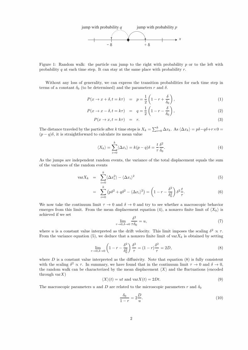
x

jump with probability pjump with probability q

+ δ� δ

Figure 1: Random walk: the particle can jump to the right with probability p or to the left withprobability q at each time step. It can stay at the same place with probability r.

Without any loss of generality, we can express the transition probabilities for each time step interms of a constant δ0 (to be determined) and the parameters r and δ.

P (x → x+ δ, t = kτ) = p =1

2

(

1− r +δ

δ0

)

, (1)

P (x → x− δ, t = kτ) = q =1

2

(

1− r − δ

δ0

)

, (2)

P (x → x, t = kτ) = r. (3)

The distance traveled by the particle after k time steps isXk =∑k

i=0 ∆xk. As 〈∆xk〉 = pδ−qδ+r×0 =(p− q)δ, it is straightforward to calculate its mean value

〈Xk〉 =k∑

i=0

〈∆xi〉 = k(p− q)δ =t

τ

δ2

δ0. (4)

As the jumps are independent random events, the variance of the total displacement equals the sumof the variances of the random events

varXk =

k∑

i=0

〈∆x2i 〉 − 〈∆xi〉2 (5)

=

k∑

i=0

(

pδ2 + qδ2 − 〈∆xi〉2)

=

(

1− r − δ2

δ20

)

δ2t

τ. (6)

We now take the continuum limit τ → 0 and δ → 0 and try to see whether a macroscopic behavioremerges from this limit. From the mean displacement equation (4), a nonzero finite limit of 〈Xk〉 isachieved if we set

limτ→0,δ→0

δ2

τδ0= u, (7)

where u is a constant value interpreted as the drift velocity. This limit imposes the scaling δ2 ∝ τ .From the variance equation (5), we deduce that a nonzero finite limit of varXk is obtained by setting

limτ→0,δ→0

(

1− r − δ2

δ20

)

δ2

τ= (1− r)

δ2

τ= 2D, (8)

where D is a constant value interpreted as the diffusivity. Note that equation (8) is fully consistentwith the scaling δ2 ∝ τ . In summary, we have found that in the continuum limit τ → 0 and δ → 0,the random walk can be characterized by the mean displacement 〈X〉 and the fluctuations (encodedthrough varX)

〈X〉(t) = ut and varX(t) = 2Dt. (9)

The macroscopic parameters u and D are related to the microscopic parameters r and δ0

δ01− r

= 2D

u. (10)

2

So, the knowledge of the macroscopic behavior of the particle leads to partial information on thelocal behavior: the parameters r and δ0 are linked through equation (10), but they are not uniquelydetermined.

Let us now derive the advection diffusion equation. To that end, let us consider the probability offinding the particle at position x at time t + τ . At the previous time increment, the particle was atthe same place (with probability r), at x − δ (and so jumped to the right with probability p), or atx+ δ (and so jumped to the left with probability q)

P (x, t+ τ) = rP (x, t) + pP (x− δ, t) + qP (x+ δ, t). (11)

A Taylor expansion (order 2 in space, order 1 in time, higher orders leads to vanishingly small values)leads to

P (x, t) + τ∂

∂tP (x, t) = rP (x, t) + p

(

P (x, t)− δ∂

∂xP (x, t) +

δ2

2

∂2

∂x2P (x, t)

)

+ q

(

P (x, t) + δ∂

∂xP (x, t) +

δ2

2

∂2

∂x2P (x, t)

)

. (12)

Collecting the terms, we get

∂

∂tP (x, t) = − δ

τ(p− q)

∂

∂xP (x, t) +

δ2

2τ(p+ q)

∂2

∂x2P (x, t) (13)

In the continuum limit, making use of equation (7) and equation (8) leads to the desired result

∂

∂tP (x, t) = −u

∂

∂xP (x, t) +D

∂2

∂x2P (x, t) (14)

The derivation above holds for D > 0. For D = 0 (pure advection), the expression of the transitionprobabilities must be changed into

P (x → x+ δ, t = kτ) = p =1

2(1− r1 + r2) , (15)

P (x → x− δ, t = kτ) = q =1

2(1− r1 − r2) , (16)

P (x → x, t = kτ) = r1. (17)

where r1 and r2 are constant parameters. The mean displacement 〈Xk〉 = k(p− q)δ admits a nonzerofinite value if we set

limτ→0,δ→0

r2δ

τ= u, (18)

implying the scaling δ ∝ τ . The variance become vanishing small

limτ→0,δ→0

varXk = limτ→0,δ→0

δ2

τ(1 − r1 + r2)t = 0. (19)

In that case, the governing equation at the macroscopic scale is the advection equation

∂

∂tP (x, t) = −u

∂

∂xP (x, t). (20)

2 Approximation of the forward Kolmogorov equation

An approximation of the forward Kolmogorov equation (11) in the paper

∂P

∂t(n; t) =

M∑

i=1

(ni + 1)(P (n+ rii+1, t)νi + P (n+ r

+i , t)σi) (21)

+P (n+ r−i , t)(λi + µi(ni − 1))

+P (n+ ri−1i , t)νi−1ni−1

−P (n, t)(νi−1ni−1 + λi + µini+1 + νini + σini).

3

can be found by transforming the discrete probabilities into continuous probability density functionsand using Taylor expansions

P (· · · , ni + 1, · · · ) = P (· · · , ni, · · · ) +∂P

∂Ni+

1

2

∂2P

∂N2i

, (22)

and in doing so, we can approximate the forward Kolmogorov equation by a multidimensional Langevinor Fokker-Planck equation. To that end, we first calculate the mean change of state per unit time

A =1

dtE(∆n) =

1

dt

3∑

k=1

pk∆n =

...νini−1 + λi + (µi − σi − νi+1)ni

...

(23)

We also calculate the covariance matrix

B =1

dtE(∆n∆n

†) (24)

=1

dt

3∑

k=1

pk∆n∆n†

=

. . .. . .

. . .. . .

. . .

· · · 0 −νini−1 νini−1 + λi + (µi + σi + νi+1)ni −νi+1ni 0 · · ·· · · . . .

. . .. . .

. . .

Using Taylor expansions of P , it can be shown that the forward Kolmogorov equation (21) can beapproximated by the Langevin equation (Allen, 2007)

dN = Adt+B1/2dW and N ≥ 0, (25)

where W is a vector of length M whose entries are independent Wiener process and B1/2 denotes

the square root of B. The square root of the tridiagonal matrix B may be tractable analytically,but it involves intense calculations for high-dimension problems (Vandebril et al., 2008). To simplifythe calculations, we follow Gillespie (2001) and write the covariance matrix B as the product of anM × (3M + 1) matrix C

B = C ·C†, (26)

with

C =

√ν1n0

√α1 −√

σ1n1 −√ν2n1 0 0 0 0 . . .

0 0 0√ν2n1

√α2 −√

σ2n2 −√ν3n2 0 . . .

...0 . . . 0

√νMnM−1

√αM −√

σMnM −√νM+1nM

, (27)

with αi = λi + µini In other words, we can write the entries of C for 1 < i < M :

• For j ≤ 3(i− 1), then Cij = 0.

• There are four nonzero entries: Ci,3i−2 =√νini−1, Ci,3i−1 =

√λi + µini, Ci,3i = −√

σini, andCi,3i+1 = −√

νi+1ni.

• For j > 3i+ 1, then Cij = 0.

Let us now consider that W is a vector of length 3M + 1 whose entries are independent Wienerprocess, then with no loss of generality, we can transform equation (25) into

dN = Adt+C · dW and N ≥ 0, (28)

This system of equations can be solved numerically (see section 5).

4

3 Poisson representation and exact Langevin equations

Here we show how to solve the forward Kolmogorov equation (21) using the Poisson representation,which is an exact technique in contrast with the approximate technique seen above. In both cases, weend up with Langevin equations, but not in the same functional space.

3.1 Generating functions

In our last paper (Ancey and Heyman, 2014), we followed Gardiner (1983) and introduced the Poissonrepresentation, which is an exact technique to transform master equations involving discrete prob-abilities into Fokker-Planck equations involving continuous probabilities. The technique consists ofintroducing the generating function and determining the dual operator associated with it.

For one-variable problems, the generating function is

G(s, t) =

∞∑

n=0

snP (n, t). (29)

Simple algebraic manipulations allow us to pass from the forward Kolmogorov equation (21) to apartial differential equation for G. For instance, whenever we meet terms like (n+ 1)P (n+ 1, t), thecorresponding term of the generating function is

∞∑

n=0

(n+ 1)snP (n+ 1, t) =∂G

∂s. (30)

In short, we thus have the following rules

(n+ 1)P (n+ 1, t) → ∂G

∂s,

P (n− 1, t) → sG,

nP (n, t) → s∂G

∂s.

For M -dimension problems, the generating function is

G(s, t) =

∞∑

n1=0

∞∑

n2=0

· · ·∞∑

nM=0

M∏

i=1

sni

i P (n, t). (31)

When multiplying the master equation (21) by sni

i and summing, the terms like

niP (· · · , ni−1, ni + 1, ni+1 − 1, ni+2, · · · )

become si+1∂siG. Similarly, terms like

niP (· · · , ni−1, ni, ni+1, ni+2, · · · )

become si∂siG. With these rules in mind, we can transform equation (21) into

∂

∂tG =

M∑

i=1

[

λi(si − 1) +(

σi + µis2i + νi+1si+1 − (σi + µi + νi)si

) ∂

∂siG

]

(32)

3.2 Poisson representation

The advection equation (32) is quite complicated to analyze and solve for multi-variable systems.Another more instructive form can be derived using the Poisson representation, a sort of Laplacetransform (Gardiner , 1983). We expand the state probability as a superposition of Poisson processesof rate a = (ai)

P (n, t) =

∫

ai

M∏

i=1

e−aiani

i

ni!f(a, t)dαi (33)

5

where f(a, t) is the probability density function of ai in cell i. The generating function (31) can bewritten

G(s, t) =

∫

ai

exp

(

−M∑

i=1

ai(si − 1)

)

f(a, t)dαi (34)

which can be seen as the scalar product (in an appropriate functional space)

G(s, t) = {K, g} , where K = exp

(

−M∑

i=1

ai(si − 1)

)

(35)

is the Laplace kernel function. The differential problem (32) can be written in the form of a linearoperator Ls(G) acting on G

∂

∂tG = Ls(G), (36)

where

Ls(G) =

M∑

i=1

[

λi(si − 1) +(

σi + µis2i + νi+1si+1 − (σi + µi + νi)si

) ∂

∂siG

]

.

As G = {K, f}, we have{

K,∂

∂tf

}

= {Ls[K(s,a)], f(a, t)} , (37)

which is equivalent to{

K,∂

∂tf

}

= {K(s,a),Ma[f(a, t)]} , (38)

where

Ma[f ] =

M∑

i=1

µi∂2aif

∂a2i− ∂

∂ai[(λi − ai(σi + νi − µi))f ] + νi+1

∂aif

∂ai+1(39)

is the adjoint of Ls(G). The governing equation for f is thus a Fokker-Planck equation

∂

∂tf = Ma[f ] = −

M∑

i=1

∂

∂ai[Aif ] +

1

2

M∑

i=1

∂2

∂a2i[Bif ], (40)

with the drift and diffusion functions

Ai = λi − κiai − (νiai − νi−1ai−1),

Bi = 2µiai,

where κi = σi − µi.

4 Analysis of the Langevin representation of b

The Fokker-Planck equation (40) is equivalent to the system of Langevin equations

dai = (λi − κai − (νiai − νi−1ai−1)) dt+√

2µaidWi (41)

As we stated in the paper, it is very tempting to take the continuum limit of equation (41) by taking∆x → 0

∂b

∂t= λ− κb− ∂

∂x(upb) +

√

2µbξb (42)

where κ(x, t) = σ − µ and λ are a smooth functions, b(x, t) is a continuous function such that b(xi) =ai/∆x in the limit of ∆x → 0 and ξb is a Gaussian noise term such that 〈ξb(x, t)ξb(x′, t′)〉 = δ(x −x′)δ(t− t′). This equation can be averaged

∂

∂t〈b〉 = λ− κ〈b〉 − ∂

∂x(up〈b〉), (43)

6

which is an advection equation with a source term. It admits a homogeneous steady-state solution

〈b〉ss =λ

κ. (44)

Far from the boundaries, there is a homogeneous regime, in which the function b(x, t) fluctuatesrandomly around 〈b〉ss. What is the variance of these fluctuations? Let us introduce the productg(x, x′, t) = b(x, t)b(x′, t). Making use of the Ito rule for the differential of dg (Gardiner , 1983), we get

dg =

[(

λ− κb− ∂upb

∂x

)

b(x′, t) (45)

+

(

λ− κb(x′, t)− ∂upb′

∂x′

)

b(x, t)

+ µ(b(x′, t) + b(x, t))δ(x − x′)] dt

+ b(x′, t)√

2µb(x, t)ξb(x, t) + b(x, t)√

2µb(x′, t)ξb(x′, t)

Taking the ensemble average and assuming homogeneous conditions (〈b(x, t)〉 = 〈b(x′, t)〉 and up

uniformly constant) state gives

∂〈g〉∂t

= 2λ〈b〉 − 2κ〈g〉+ up

(

∂

∂x+

∂

∂x′

)

〈g〉+ 2µ〈b〉δ(x′ − x). (46)

Under spatially homogeneous conditions, 〈g〉 depends only on r = x′ − x. The change of variablesx → x and x′ → x+ r leads to

∂

∂x′=

∂

∂rand

∂

∂x=

∂

∂x− ∂

∂r(47)

We end up with the following governing equation for 〈g〉∂〈g(r, t)〉

∂t= 2λ〈b〉ss − 2κ〈g〉+ 2µ〈b〉ssδ(r), (48)

where the gradient terms have cancelled out.For steady state conditions (∂t〈g(r, t)〉ss = 0), we find that the spatial correlation is

〈g〉 = λ+ µδ(r)

κ〈b〉ss, (49)

from which we deduce the second order moment

〈g(0)〉ss =λ+ µδ(0)

κ〈b〉ss = λ

λ+ µδ(0)

κ2, (50)

and the variance of b under steady state conditions

var ssb = 〈g(0)〉ss − 〈b〉2ss =λµ

κ2δ(0). (51)

5 Euler scheme for solving the Langevin equation for ai

The Euler (or Euler-Maruyama) approximation of the Langevin equation

dai(t) = (λi − ai(σi − µi) + νi−1ai−1 − νiai) dt+√

2µiai dWi(t), (52)

(with an appropriate initial condition) is the iterative scheme (Higham, 2001; Iacus , 2008)

Ak+1i = Ak

i +(

λi − (κi − νi)Aki + νi−1A

ki−1

)

∆t+√

2µiAi (Zk+1i − Zk

i ), (53)

where Aki = ai(tk) and Zk

i (t) = W ki (tk). The discrete times are tk = tk+1 +∆t.

In practice the random terms Zk+1i − Zk

i coming from the difference of the Wiener processes are

modeled as r√∆t where r is a random number drawn from a uniform distribution (0 ≤ r ≤ 1).The

Euler scheme has order 1/2 of strong convergence, i.e. we can find a constant C such that

〈|ai(tk)−Aki |〉 < C

√∆t. (54)

7

6 Iterative calculation of the spatial cross correlations

We have found

var b =µ

κ〈b〉ssδ(0) =

µλ

κ2, (55)

which is independent of up! What goes awry with this theory?Let us return to the discretized equations (41) and let us calculate the second-order moment

(making use of the Ito rule)

d

dt〈a2i 〉 = 2λ〈ai〉 − 2(κ+ ν)〈a2i 〉+ 2ν〈aiai−1〉+ 2µ〈ai〉 (56)

which involves the unknown cross correlation 〈aiai−1〉. Assuming homogeneous steady-state conditions(λ〈ai〉 = λ〈a〉, no time dependence), this equation yields

0 = 2λ〈a〉ss − 2(κ+ ν)〈a2〉ss + 2ν〈aiai−1〉ss + 2µ〈a〉ss (57)

An evolution equation for the correlation 〈aiai−1〉 is

d

dt〈aiai−1〉 = λ(〈ai〉+ 〈ai−1〉)− 2(κ+ ν)〈aiai−1〉+ ν〈a2i−1〉+ ν〈aiai−2〉 (58)

which under steady-state conditions gives

0 = 2λ〈a〉ss − 2(κ+ ν)〈aiai−1〉ss + ν〈a2〉ss + ν〈aiai−2〉ss, (59)

which depends 〈aiai−2〉ss. To close the system, let us assume that this term ν〈aiai−2〉ss is zero, then

〈aiai−1〉ss =λ

κ+ ν〈a〉ss +

ν

2(κ+ ν)〈a2〉ss, (60)

and after substitution into equation (57), we get

2(κ+ ν)〈a2〉ss = 2(λ+ µ)〈a〉ss + 2ν

(

λ

κ+ ν〈a〉ss +

ν

2(κ+ ν)〈a2〉ss

)

that is(

2(κ+ ν)− ν2

κ+ ν

)

〈a2〉ss = 2

(

λ+ µ+ νλ

κ+ ν

)

〈a〉ss

from which we deduce the following approximation of the variance

var ss a =2(λ+ µ)(κ+ ν) + νλ

2(κ+ ν)2 − ν2λ

κ−(

λ

κ

)2

=λµ

(κ+ ν)2

(

1 +ν

κ+ ν+

1

2

(

3− λ

µ

)

ν2

(κ+ ν)2+O(ν2)

)

,

(61)which depends on ν and gives equation (55) in the limit ν → 0.

Higher-order approximations can be obtained iteratively by calculating the correlations

〈aiai−k〉ss =λ

κ+ ν〈a〉ss +

ν

2(κ+ ν)〈aiai−k+1〉ss +

ν

2(κ+ ν)〈aiai−k−1〉ss, (62)

and closing the system by assuming that at order K, the last correlation term 〈aiai−K−1〉ss is zero.Figure 2 shows the variation of var a with the emigration rate ν. There is clearly a significant effect

of ν: the variance of a decreases with increasing ν. The higher the emigration rate, the higher theorder of the approximate solution required to get a sufficiently accurate estimate of var a. Note thanwhen ν approaches the CFL limit (∆t)−1 = 100 s−1, the simulation blows up.

8

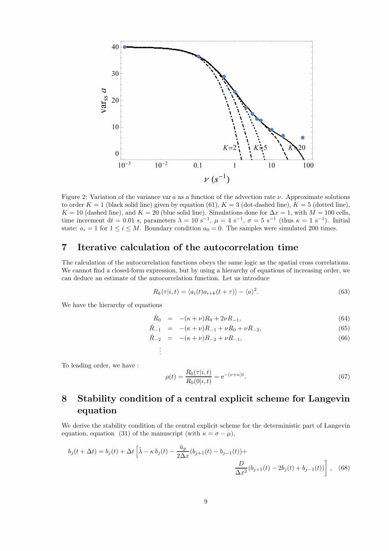
Figure 2: Variation of the variance var a as a function of the advection rate ν. Approximate solutionsto order K = 1 (black solid line) given by equation (61), K = 3 (dot-dashed line), K = 5 (dotted line),K = 10 (dashed line), and K = 20 (blue solid line). Simulations done for ∆x = 1, with M = 100 cells,time increment dt = 0.01 s, parameters λ = 10 s−1, µ = 4 s−1, σ = 5 s−1 (thus κ = 1 s−1). Initialstate: ai = 1 for 1 ≤ i ≤ M . Boundary condition a0 = 0. The samples were simulated 200 times.

7 Iterative calculation of the autocorrelation time

The calculation of the autocorrelation functions obeys the same logic as the spatial cross correlations.We cannot find a closed-form expression, but by using a hierarchy of equations of increasing order, wecan deduce an estimate of the autocorrelation function. Let us introduce

Rk(τ |i, t) = 〈ai(t)ai+k(t+ τ)〉 − 〈a〉2. (63)

We have the hierarchy of equations

R0 = −(κ+ ν)R0 + 2νR−1, (64)

R−1 = −(κ+ ν)R−1 + νR0 + νR−2, (65)

R−2 = −(κ+ ν)R−2 + νR−1, (66)

...

To leading order, we have :

ρ(t) =R0(τ |i, t)R0(0|i, t)

= e−(ν+κ)t. (67)

8 Stability condition of a central explicit scheme for Langevin

equation

We derive the stability condition of the central explicit scheme for the deterministic part of Langevinequation, equation (31) of the manuscript (with κ = σ − µ),

bj(t+∆t) = bj(t) + ∆t[

λ− κ bj(t)−up

2∆x(bj+1(t)− bj−1(t))+

D

∆x2(bj+1(t)− 2bj(t) + bj−1(t))

]

, (68)

9

that can be rewritten as

bn+1j = bnj−1

(

r +ζ

2

)

+ bnj (1− 2r − κ∆t) + bnj−1

(

r − ζ

2

)

+ λ∆t (69)

with

r ≡ D∆t

∆x2, ζ ≡ up

∆t

∆xbn+1j = bj(t+∆t) , bnj = bj(t) . (70)

To this end, a von Neumann stability analysis is performed on the base solution b = λ/κ. Intro-ducing an exponential perturbation,

bnj =λ

κ+ ei j ∆x ξ , bn+1

j =λ

κ+ g(ξ) ei j ∆x ξ , i =

√−1 , (71)

into equation (69), we arrive at the dispersion relation

g(ξ) ei j ∆x ξ = ei j ∆x ξ

[

1− κ∆t+ r(e−i∆x ξ − 2 + ei∆x ξ) +ζ

2(e−i∆x ξ − ei∆x ξ)

]

. (72)

The amplification factor is therefore

g(ξ) = 1− κ∆t+ 2 r [−1 + cos(ξ∆x)] − i ζ sin(ξ∆x) . (73)

The method is stable if g(ξ) lies inside the unitary circle in the complex plane, i.e. if |g(ξ)| ≤ 1.Taking into account that −2 ≤ cos(ξ∆x)− 1 ≤ 0 and −1 ≤ sin(ξ∆x) ≤ 1, the method is stable if thefollowing condition holds:

max{(1− κ∆t− 4 r)2 + ζ2, (1− κ∆t)2 + ζ2} ≤ 1 . (74)

Substituting the definitions of r and ζ (70) into equation (74) and solving for ∆t, we arrive at thestability condition for the time step

∆t ≤ min

{

(2 κ∆x2 + 8D)∆x2

κ2∆x4 + (u2p + 8 κD)∆x2 + 16D2

,2 κ∆x2

κ2∆x2 + u2p

}

. (75)

Therefore, the method is conditionally stable.We can check that equation (75) correctly predicts well known results in simpler cases:

• The second order centred scheme is unstable for the pure advection equation: setting κ = 0,λ = 0, D = 0 and up 6= 0 in equation (75), it follows ∆t ≤ 0. Therefore, the scheme isunconditionally unstable at all ∆t.

• In the pure diffusive case (i.e. κ = 0, λ = 0, up = 0, D 6= 0) we recover the diffusion stabilitycondition of explicit schemes ∆t ≤ ∆x2/2D.

It is interesting to highlight the stabilizing effect of the parameter κ:

• In the convective-erosion-deposition case (i.e. D = 0), the scheme is conditionally stable when∆t ≤ 2κ∆x2/(κ2∆x2 + u2

p). In the limit of ∆x → 0, this condition can be approximated as∆t ≤ 2κ∆x2/u2

p − 2κ3∆x4/u4p. The leading order term ∆t ≤ 2κ∆x2/u2

p is analogous to thediffusion restriction of the time step with D = u2

p/4κ.

• Finally, for very thin meshes, ∆x → 0, equation (75) can be approximated as

∆t

∆x2≤ min

{

1

2D,2κ

u2p

}

. (76)

So the stability condition is dominated by the diffusion coefficient D and the deposition rate κin this limit.

A fully implicit scheme could be formulated to avoid the constraint on the time step. In such acase, Thomas’ algorithm could be employed to solve efficiently the tridiagonal system of equations.

10

9 Variance of diffusive processes

Let us introduce the fluctuating part b′ = b−〈b〉 in the Langevin equation (102) for b with no advectionterm (up = 0). The fluctuating part b′ satisfies

∂tb′ = d

∂2b′

∂x2− κb′ +

√

2µ(〈b〉ss + b′)ξb (77)

This Ito’s rule for the change of variable f = b′2 in equation (77) gives

df = (2b′A+ 2µb) dt+ 2b′√

2µbdW +O(dt), (78)

with A = d∂xxb− κb′. If we take the ensemble average, we end up with

∂

∂t〈b′2〉 = 2

(

d∂2

∂x2〈b′2〉 − κ〈b′2〉+ µ〈b〉

)

. (79)

We introduce the variance var b = 〈b2〉 − 〈b〉2 = 〈b′2〉 and the spatial covariance cov b = 〈b(x, t)b(x +r, t)〉−〈b〉2. Following the same reasoning that leads us to equation (79) and making use of b = b′+〈b〉ssfor the homogeneous region, we find

1

2

∂

∂tcov b = d

∂2

∂r2cov b− κcov b+ µ〈b〉ssδ(r). (80)

This equation is characterized by its steady steady Fourier spectrum

−ω2dF − κF + µ〈b〉ss = 0, (81)

where

F [f ] =

∫ ∞

−∞

e−ıωsf(s)ds. (82)

denotes the Fourier transform. The solution to this algebraic equation is straightforward

F(ω) =µ〈b〉ssκ+ dω2

. (83)

Taking the inverse Fourier transform leads to

cov ssb =1

2

µ〈b〉ssκℓc

e−|r|/ℓc with ℓc =

√

d

κ, (84)

from which we deduce the variance by taking r = 0

var ssb =1

2

µ〈b〉ssκℓc

. (85)

This expression holds for ∆x → 0 (in practive, when the observation window is very small comparedto the correlation length ℓc). It may be interesting to calculate an average variance over a controlvolume of arbitrary length ∆x

var ssb =1

∆x2

1

2

µ〈b〉ssκℓc

∫

∆x

∫

∆x

e−|x−x′|/ℓcdxdx′,

=µλ

κ2

ℓc∆x2

(

∆x

ℓc+ exp

(

−∆x

ℓc

)

− 1

)

. (86)

Naturally, in the limit ∆x → 0, we retrieve the local variance (85).

11

10 Simulation of advection and diffusion

Here we show numerical simulations of the Langevin equations

dai(t) = (λi − ai(σi − µi) + νi−1ai−1 − νiai (87)

+ di(ai+1 + ai−1 − 2ai)) dt+√

2µiai dWi(t).

We solved this system of Langevin equations numerically using an Euler scheme with time step dt =0.01 s (see section 5) (Higham, 2001; Iacus , 2008). The computational domain was split into M = 100cells of length ∆x = 1 m.

We solved an initial boundary value problem with the initial condition ai(0) = 1. We imposedboundary conditions on the left and the right with ghost cells: a0 = 0 and aM+1 = aM . We usedthe same parameters λ = 10 s−1, σ = 5 s−1, µ = 4 s−1, d = 1 m s−2. For the advection rate, wetook ν = 1 s−1, ν = 5 s−1, and ν = 10 s−1. The dots and gray lines show the numerical simulations.Averages and probabilities were computed over 500 samples once the steady state has been reached(in practice for t ≥ 10 s).

The mean behavior is obtained by taking the continuum limit

∂

∂tb(x, t) +

∂

∂x(upb) =

∂2

∂x2(Db) + λ− (σ − µ)b+

√

2µb ξb, (88)

(with D = lim∆x→0∆x2di), then the ensemble average

∂

∂tc(x, t) +

∂

∂x(upc) = s(c) +

∂2

∂x2(Dc), (89)

subject to c(x, 0) = 1 and the following boundary condition on the left of the domain c(0, t) = 0 and∂xc(L, t) = 0 with L = M∆x (these two conditions are not strictly compatible initially at x = 0). Theshorthand notation s(c) is the source term s(c) = λ′ − (σ − µ)c.

Under homogeneous steady-state conditions, we have found for the mean value, the covariance,and the variance

〈b〉ss =λ

σ − µ, covss b(r) =

1

2

µ

σ − µ

〈b〉ssℓc

exp−r/ℓc , and varss b =1

2

µ

σ − µ

〈b〉ssℓc

, (90)

with ℓc =√

D/(σ − µ) the correlation length. The autocorrelation function is

ρ(t) =1

2

(

exp

(

−Pet

tc

)

Erfc

[(

1− Pe

2

)√

t

tc

]

(91)

+ exp

(

Pet

tc

)

Erfc

[(

1 +Pe

2

)√

t

tc

])

with tc = (σ − µ)−1 the correlation time, ℓc =√

D/(σ − µ) the correlation length, and Pe = upℓc/Dthe Peclet number.

Figure 3 shows the variation of 〈ai〉ss as function of the position i at the final computation timet = 20 s. The mean behavior is correctly predicted by the advection diffusion equation (89) (we canmake the comparison directly since ∆x = 1 m and c(x, t) = p〈ai〉ss/∆x in the limit ∆xo0). There isan excellent agreement between the numerical data (dots) and the solution to the advection diffusionequation (89) for all values of ν tested. Figure 4 shows how 〈ak(t)〉 evolves with time at the middleof the computational domain. Again, there is excellent agreement between the advection diffusionequation (89) and the numerical data. As a summary, the mean behavior is well captured by theory.Figure 5 shows particular realizations.

More interestingly, Figure 6 shows the empirical distribution of the numerical data and the the-oretical gamma distribution Ga(α, β) with three sets of parameters: α = λ/µ and β = µ/(σ − µ)(dashed line) which hold for one-cell systems (Ancey and Heyman, 2014), with α = 〈a〉2ss/varss a andβ = varss a/〈a〉ss (dotted line), where varss a is deduced from the b variance in equation (86), and

α = 〈a〉2ss/varss a and β = varss a/〈a〉ss (solid line), where varss a is deduced from the b variance in

12

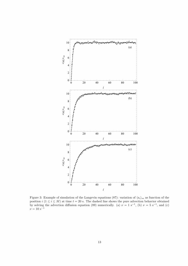
Figure 3: Example of simulation of the Langevin equations (87): variation of 〈ai〉ss as function of theposition i (1 ≤ i ≤ M) at time t = 20 s. The dashed line shows the pure advection behavior obtainedby solving the advection diffusion equation (89) numerically. (a) ν = 1 s−1, (b) ν = 5 s−1, and (c)ν = 10 s−1

13

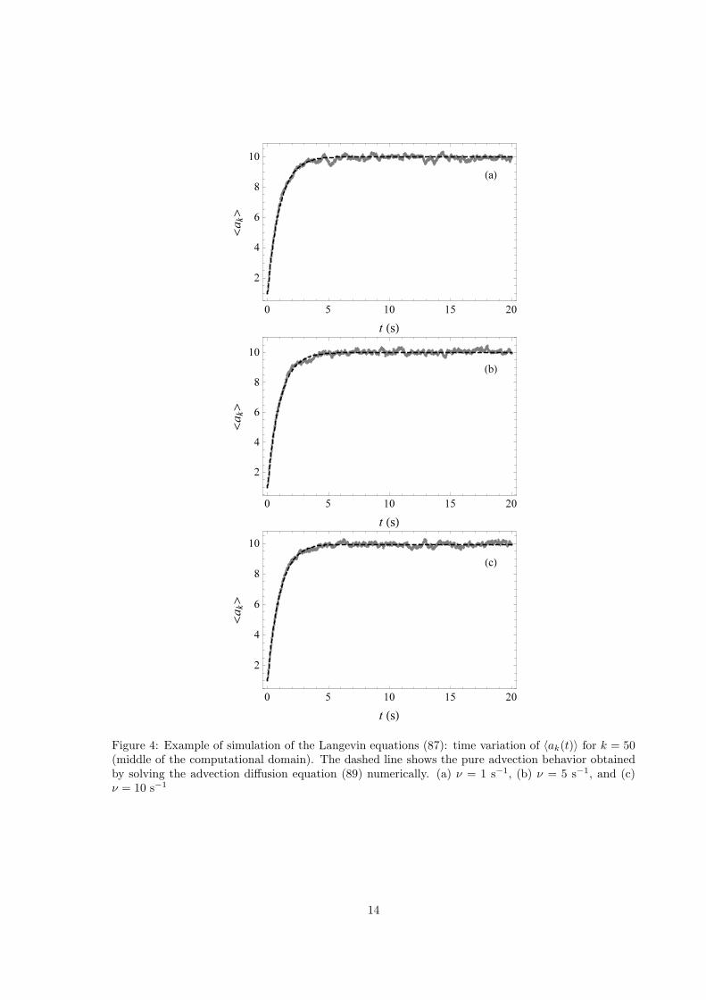
Figure 4: Example of simulation of the Langevin equations (87): time variation of 〈ak(t)〉 for k = 50(middle of the computational domain). The dashed line shows the pure advection behavior obtainedby solving the advection diffusion equation (89) numerically. (a) ν = 1 s−1, (b) ν = 5 s−1, and (c)ν = 10 s−1

14

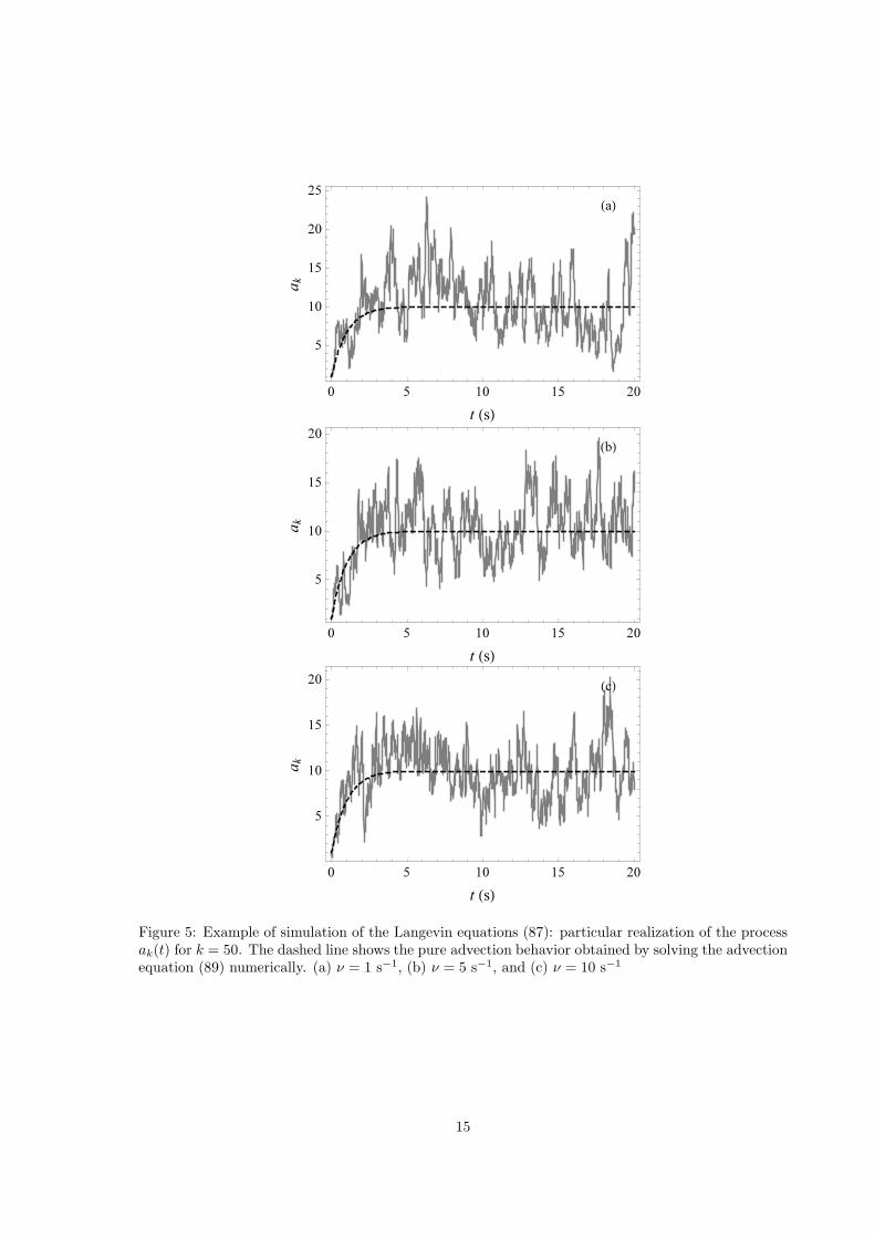
Figure 5: Example of simulation of the Langevin equations (87): particular realization of the processak(t) for k = 50. The dashed line shows the pure advection behavior obtained by solving the advectionequation (89) numerically. (a) ν = 1 s−1, (b) ν = 5 s−1, and (c) ν = 10 s−1

15

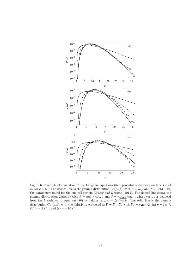
Figure 6: Example of simulation of the Langevin equations (87): probability distribution function ofak for k = 50. The dashed line is the gamma distribution Ga(α, β), with α = λ/µ and β = µ/(σ−µ),the parameters found for the one-cell system (Ancey and Heyman, 2014). The dotted line shows thegamma distribution Ga(α, β) with α = 〈a〉2ss/varss a and β = varss a/〈a〉ss, where varss a is deducedfrom the b variance in equation (86) by taking varss a = ∆x2var b. The solid line is the gamma

distribution Ga(α, β), with the diffusivity corrected as D = D+D∗ with D∗ = ν∆x2/2. (a) ν = 1 s−1,(b) ν = 5 s−1, and (c) ν = 10 s−1.

16

equation (86) but with D = D + D∗ instead of D. The one-cell solution is unable to describe theempirical distribution. For ν = 1 s−1, the difference between the two diffusion solutions is so tiny thatit is not visible. For ν = 5 s−1 and ν = 10 s−1, the differences are marked. The distribution Ga(α, β)closely matches the numerical data, confirming that particle advection produces diffusion-like effects.

Figure 7 shows the autocorrelation functions. For ν = 1 s−1, the theoretical function (91) properlydescribes the empirical autocorrelation function. For ν = 5 s−1 and ν = 10 s−1, the correctionD → D = D +D∗ provides the correct trend.

11 Analytical solution to the pure advection solution

Here we provide the analytical solution to the pure advection equation [referred to as equation (20) inthe paper]

∂

∂tc(x, t) +

∂

∂x(upc) = s(c), (92)

where the source term is s(c) = λ′ − (σ − µ)c = λ′ − κc and the advection velocity up is assumedconstant. We consider the following boundary initial value problem

c(0, t) = 0 for t ≥ 0 and c(x, 0) = f(x) for x ≥ 0, (93)

where f is a positive function satisfying f(0) = 0 for the consistency of the initial and boundaryconditions. We use the method of characteristics (Zauderer , 1983) and cast equation (92) in thefollowing form

dc

dζ= λ′ − κc along the characteristic curve

dx

dζ= up, (94)

where we have introduced the dummy variable ζ. To solve this boundary initial value problem, wetake advantage from the fact that the characteristic curves are all parallel (with slope u−1

p ). It is uspossible to break down the original problem into an initial value problem (domain 1) and a boundaryvalue problem (domain 2), as shown by Figure 8.

We first solve the system of characteristic equations for domain 1 (see Figure 8)

∂t

∂ζ= 1,

∂x

∂ζ= up and

∂c

∂ζ= s(c), (95)

with the initial data written parametrically as

x(ζ = 0) = x1, t(ζ = 0) = 0 and c(ζ = 0) = f(x1). (96)

The integration is straightforward

c1(x, t) =e−κt

κ

(

κf(x− upt) + λ′(eκt − 1))

. (97)

We now solve the system of characteristic equations for domain 2 (see Figure 8)

∂t

∂ζ= 1,

∂x

∂ζ= up and

∂c

∂ζ= s(c). (98)

The initial data for the boundary value problem can be written parametrically as

x(ζ = 0) = 0, t(ζ = 0) = t1 and c(ζ = 0) = 0. (99)

The solution is readily found

c2(x, t) =λ′

κ

(

1− exp

(

−κx

up

))

(100)

The full solution to the boundary initial value problem is thus

c(x, t) =

{

c1(x, t) for x ≥ upt,c2(x, t) for x < upt.

(101)

Figure 9 shows the exact solution to the boundary initial value problem considered in Figure 2 inthe body of the paper.

17

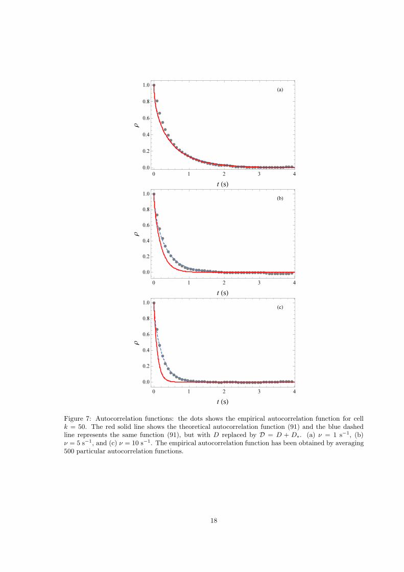
Figure 7: Autocorrelation functions: the dots shows the empirical autocorrelation function for cellk = 50. The red solid line shows the theoretical autocorrelation function (91) and the blue dashedline represents the same function (91), but with D replaced by D = D + D∗. (a) ν = 1 s−1, (b)ν = 5 s−1, and (c) ν = 10 s−1. The empirical autocorrelation function has been obtained by averaging500 particular autocorrelation functions.

18

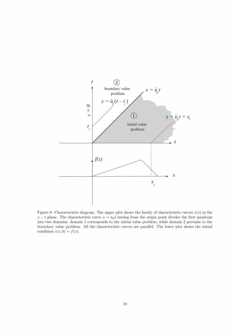
t

x

x

f(x)

initial value

problem

boundary value

problem

x = u t + xp

①

②

x1

1

x = u t p

x = u (t – t )p 1

t1

c =

0

Figure 8: Characteristic diagram. The upper plot shows the family of characteristic curves x(s) in thex− t plane. The characteristic curve x = upt issuing from the origin point divides the first quadrantinto two domains: domain 1 corresponds to the initial value problem, while domain 2 pertains to theboundary value problem. All the characteristic curves are parallel. The lower plot shows the initialcondition c(x, 0) = f(x).

19

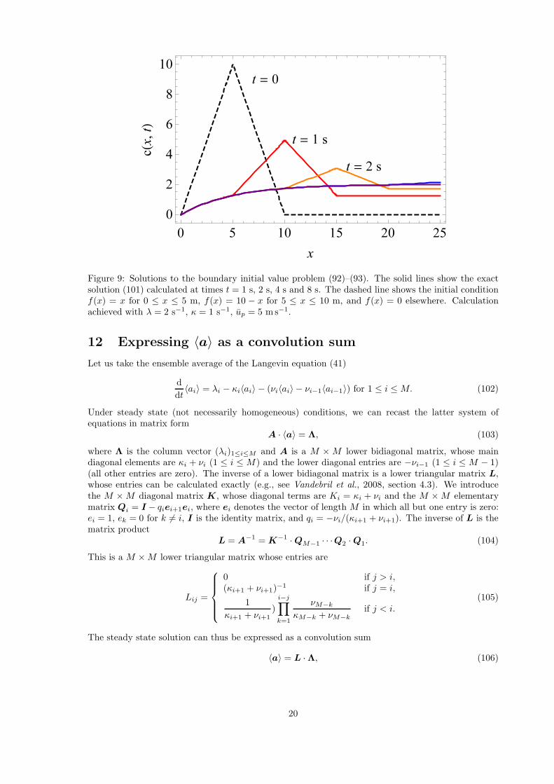
Figure 9: Solutions to the boundary initial value problem (92)–(93). The solid lines show the exactsolution (101) calculated at times t = 1 s, 2 s, 4 s and 8 s. The dashed line shows the initial conditionf(x) = x for 0 ≤ x ≤ 5 m, f(x) = 10 − x for 5 ≤ x ≤ 10 m, and f(x) = 0 elsewhere. Calculationachieved with λ = 2 s−1, κ = 1 s−1, up = 5 ms−1.

12 Expressing 〈a〉 as a convolution sum

Let us take the ensemble average of the Langevin equation (41)

d

dt〈ai〉 = λi − κi〈ai〉 − (νi〈ai〉 − νi−1〈ai−1〉) for 1 ≤ i ≤ M. (102)

Under steady state (not necessarily homogeneous) conditions, we can recast the latter system ofequations in matrix form

A · 〈a〉 = Λ, (103)

where Λ is the column vector (λi)1≤i≤M and A is a M × M lower bidiagonal matrix, whose maindiagonal elements are κi + νi (1 ≤ i ≤ M) and the lower diagonal entries are −νi−1 (1 ≤ i ≤ M − 1)(all other entries are zero). The inverse of a lower bidiagonal matrix is a lower triangular matrix L,whose entries can be calculated exactly (e.g., see Vandebril et al., 2008, section 4.3). We introducethe M ×M diagonal matrix K, whose diagonal terms are Ki = κi + νi and the M ×M elementarymatrix Qi = I − qiei+1ei, where ei denotes the vector of length M in which all but one entry is zero:ei = 1, ek = 0 for k 6= i, I is the identity matrix, and qi = −νi/(κi+1 + νi+1). The inverse of L is thematrix product

L = A−1 = K

−1 ·QM−1 · · ·Q2 ·Q1. (104)

This is a M ×M lower triangular matrix whose entries are

Lij =

0 if j > i,(κi+1 + νi+1)

−1 if j = i,

1

κi+1 + νi+1)

i−j∏

k=1

νM−k

κM−k + νM−kif j < i.

(105)

The steady state solution can thus be expressed as a convolution sum

〈a〉 = L ·Λ, (106)

20

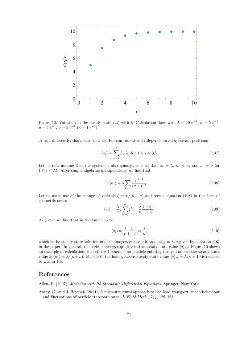
Figure 10: Variation in the steady state 〈ai〉 with i. Calculation done with λ = 10 s−1, σ = 5 s−1,µ = 4 s−1, ν = 5 s−1 (κ = 1 s−2).

or said differently, this means that the Poisson rate at cell i depends on all upstream positions

〈ai〉 =i∑

k=1

Lijλj for 1 ≤ i ≤ M. (107)

Let us now assume that the system is also homogeneous so that λi = λ, κi = κ, and νi = ν for1 ≤ i ≤ M . After simple algebraic manipulations, we find that

〈ai〉 = λ

i∑

k=1

νk−1

(κ+ ν)k. (108)

Let us make use of the change of variable ζ = ν/(κ + ν) and recast equation (108) in the form ofgeometric series

〈ai〉 =λ

νζ

i−1∑

k=0

ζk =λ

ν

1− ζi

1− ζ. (109)

As ζ < 1, we find that in the limit i → ∞,

〈ai〉 ≈λ

ν

ζ

1− ζ=

λ

κ, (110)

which is the steady state solution under homogeneous conditions, 〈a〉ss = λ/κ given by equation (16)in the paper. In general, the series converges quickly to the steady state value 〈a〉ss. Figure 10 showsan example of calculation: for cell i = 1, there is no particle entering this cell and so the steady statevalue is 〈a1〉 = λ/(κ+ ν). For i > 6, the homogeneous steady-state value 〈a〉ss = λ/κ = 10 is reachedto within 1%.

References

Allen, E. (2007), Modeling with Ito Stochastic Differential Equations, Springer, New York.

Ancey, C., and J. Heyman (2014), A microstructural approach to bed load transport: mean behaviourand fluctuations of particle transport rates, J. Fluid Mech., 744, 129–168.

21

Gardiner, C. (1983), Handbook of Stochastic Methods, Springer Verlag, Berlin.

Gillespie, D. (2001), Approximate accelerated stochastic simulation of chemically reacting systems, J.Chem. Phys., 115, 1716–1733.

Higham, D. (2001), An algorithmic introduction to numerical simulation of stochastic differentialequations, SIAM Rev., 43, 525–546.

Iacus, S. (2008), Simulation and Inference for Stochastic Differential Equations, Springer, New York.

Vandebril, R., M. Van Barel, and N. Mastronardi (2008), Matrix Computations and Semiseparable

Matrices, Volume 1: Linear Systems, The Johns Hopkins University Press, Baltimore.

Zauderer, E. (1983), Partial Differential Equations of Applied Mathematics, Pure and Applied Math-ematics, John Wiley & Sons, New York.

22

Stochastic interpretation of the advection diﬀusion...

Documents

Transcript of Stochastic interpretation of the advection diﬀusion...