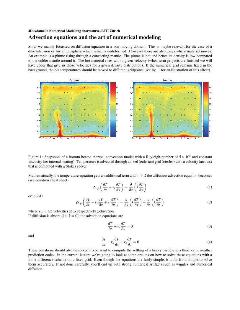
4D-Adamello Numerical Modelling shortcourse–ETH Zurich

Advection equations and the art of numerical modelingSofar we mainly focussed on diffusion equation in a non-moving domain. This is maybe relevant for the case of adike intrusion or for a lithosphere which remains undeformed. However there are also cases where material moves.An example is a plume rising through a convecting mantle. The plume is hot and hence its density is low comparedto the colder mantle around it. The hot material rises with a given velocity (when term-projects are finished we willhave codes that give us those velocities for a given density distribution). If the numerical grid remains fixed in thebackground, the hot temperatures should be moved to different gridpoints (see fig. 1 for an illustration of this effect).

Figure 1: Snapshots of a bottom heated thermal convection model with a Rayleigh-number of 5× 105 and constantviscosity (no internal heating). Temperature is advected through a fixed (eulerian) grid (circles) with a velocity (arrows)that is computed with a Stokes solver.

Mathematically, the temperature equation gets an additional term and in 1-D the diffusion-advection equation becomes(see equation cheat sheet)

ρcp

(∂T∂t

+ vx∂T∂x

)=

∂

∂x

(k

∂T∂x

)(1)

or in 2-D

ρcp

(∂T∂t

+ vx∂T∂x

+ vz∂T∂z

)=

∂

∂x

(k

∂T∂x

)+

∂

∂z

(k

∂T∂z

)(2)

where vx,vz are velocities in x-,respectively z-direction.If diffusion is absent (i.e. k = 0), the advection equations are

∂T∂t

+ vx∂T∂x

= 0 (3)

and∂T∂t

+ vx∂T∂x

+ vz∂T∂z

= 0 (4)

These equations should also be solved if you want to compute the settling of a heavy particle in a fluid, or in weatherprediction codes. In the current lecture we’re going to look at some options on how to solve these equations with afinite difference scheme on a fixed grid. Even though the equations are fairly simple, it is far from simple to solvethem accurately. If not done carefully, you’ll end up with strong numerical artifacts such as wiggles and numericaldiffusion.

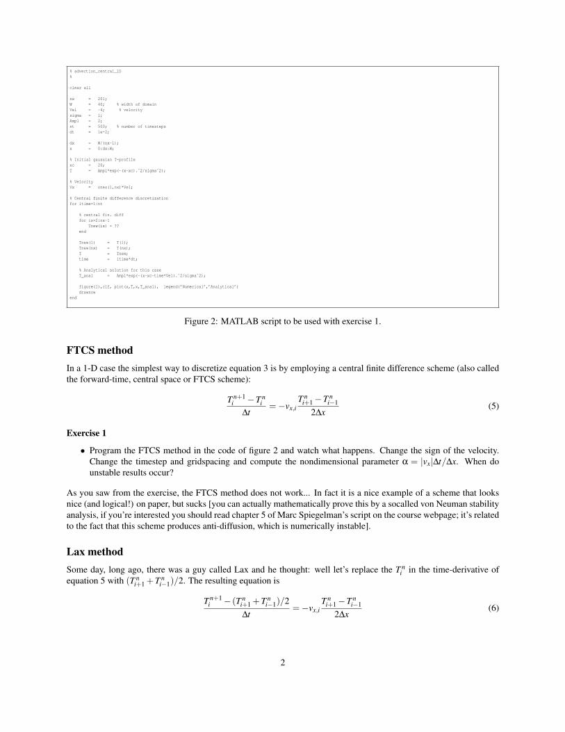
% advection_central_1D%

clear all

nx = 201;W = 40; % width of domainVel = -4; % velocitysigma = 1;Ampl = 2;nt = 500; % number of timestepsdt = 1e-2;

dx = W/(nx-1);x = 0:dx:W;

% Initial gaussian T-profilexc = 20;T = Ampl*exp(-(x-xc).ˆ2/sigmaˆ2);

% VelocityVx = ones(1,nx)*Vel;

% Central finite difference discretizationfor itime=1:nt

% central fin. difffor ix=2:nx-1

Tnew(ix) = ??end

Tnew(1) = T(1);Tnew(nx) = T(nx);T = Tnew;time = itime*dt;

% Analytical solution for this caseT_anal = Ampl*exp(-(x-xc-time*Vel).ˆ2/sigmaˆ2);

figure(1),clf, plot(x,T,x,T_anal), legend(’Numerical’,’Analytical’)drawnow

end

Figure 2: MATLAB script to be used with exercise 1.

FTCS methodIn a 1-D case the simplest way to discretize equation 3 is by employing a central finite difference scheme (also calledthe forward-time, central space or FTCS scheme):

T n+1i −T n

i∆t

=−vx,iT n

i+1−T ni−1

2∆x(5)

Exercise 1

• Program the FTCS method in the code of figure 2 and watch what happens. Change the sign of the velocity.Change the timestep and gridspacing and compute the nondimensional parameter α = |vx|∆t/∆x. When dounstable results occur?

As you saw from the exercise, the FTCS method does not work... In fact it is a nice example of a scheme that looksnice (and logical!) on paper, but sucks [you can actually mathematically prove this by a socalled von Neuman stabilityanalysis, if you’re interested you should read chapter 5 of Marc Spiegelman’s script on the course webpage; it’s relatedto the fact that this scheme produces anti-diffusion, which is numerically instable].

Lax methodSome day, long ago, there was a guy called Lax and he thought: well let’s replace the T n

i in the time-derivative ofequation 5 with (T n

i+1 +T ni−1)/2. The resulting equation is

T n+1i − (T n

i+1 +T ni−1)/2

∆t=−vx,i

T ni+1−T n

i−1

2∆x(6)

2

Exercise 2

• Program the Lax method by modifying the script of the last exercise. Play with different velocities and computethe Courant number α, which is given by the following equation:

α =∆x

∆t|vx|(7)

Is the numerical scheme stable for all Courant numbers?

As you saw from the exercise the Lax method doesn’t blow up, but does have a lot of numerical diffusion. So it’s animprovement but it’s still not perfect, since you may loose the plumes of figure 1 around mid-mantle purely due tonumerical diffusion (and than you’ll probably find some fancy geochemical explanation for this...). I hope that youalso slowly start to see that numerical modeling is a bit of an art...

Upwind schemeThe next scheme that people came up with is the so-called upwind scheme. Here, the spatial finite difference schemedepends on the sign of the velocity:

T n+1i −T n

i∆t

=−vx,i

{T n

i −T ni−1

∆x , if vx,i > 0T n

i+1−T ni

∆x , if vx,i < 0(8)

Exercise 3

• Program the upwind scheme method. Play with different velocities and compute the Courant number α Is thenumerical scheme stable for all Courant numbers?

Also the upwind scheme suffers from numerical diffusion.Sofar we employed explicit discretizations. You’re probably wondering whether implicit discretizations will save

us again this time. Bad news: doesn’t work (try if you want). So we have to come up with something else.

Staggered LeapfrogThe explicit discretizations discussed sofar were second order accurate in time, but only first order in space. We canalso come up with a scheme that is second order in time and space

T n+1i −T n−1

2∆t=−vx,i

T ni+1−T n

i−1

2∆x(9)

the difficulty in this scheme is that we’ll have to store two timestep levels: both T n−1 and T n (but i’m sure you’llmanage).

Exercise 4

• Program the staggered leapfrog method (assume that at the first timestep T n−1 = T n). Play around with differentvalues of the Courant number α. Also make the width of the gaussian curve smaller.

The staggered leapfrog method works quite well regarding the amplitude and wavespeed as long as α is closeto one. If however α << 1 and the lengthscale of the to-be-transported quantity is small compared to the numberof gridpoints (e.g. we have a thin plume), numerical oscillations again occur. This is typically the case in mantleconvection simulations (see Fig. 1), so again we have a numerical scheme that’s not great for mantle convectionsimulations.

3

MPDATAThis is a technique that is frequently applied in (older) mantle convection codes. The basic idea is based on an ideaof Smolarkiewicz and is basically a modification of the upwind scheme, where some iterative corrections are applied.The results are quite ok. However it’s somewhat more complicated to implement (the system that’s solved is actuallynonlinear and requires iterations, which we did not discuss yet). Moreover we still have a restriction on the timestep(given by the Courant criterium). For this reason we won’t go into detail here (see Spiegelman’s lecture notes, chapter5 if you’re interested).

Marker-based advectionSo what we want is a scheme that doesn’t blow up, has only small numerical diffusion and that is not limited bythe Courant criterium. The simplest manner in doing this is to use a marker-based or tracer-based advection scheme,which -as a nice side-effect- is something you will anyways need to model geodynamic case studies (as soon as youfinished the Stokes solver in one of the next classes).

Basic idea

The basic idea of a marker-based advection method that you add some marker in your code (typically many more thanthe number of numerical gridpoints). A marker is a point, which has coordinates ([x] in 1D, [x,y] in 2D) and a giventemperature T . You define your initial temperature field at each marker.

Marker-based advection, than requires the following steps:

1. Interpolate velocity from nodal points to marker. In matlab, the command interp1 (in 1D) or interp2 (in 2D) canbe used to do this.

2. Compute the new marker location with xn+1(p) = xn(p)+∆tvnx(p) (where vn

x(p) is the velocity at marker p).

3. Check for markers that are outside the boundary of the computational model.

4. Interpolate temperature from markers to nodal points. If nodal points have the coordinates x(i), x(i+1), x(i+2),...a possibility to do this is to find all markers between x(i-1/2) and x(i+1/2) (use ’find’), and compute the averagetemperature among those particles (use ’mean’ to do this). More sophisticated schemes involve distance-basedaveraging (see lecture notes of Taras Gerya).

5. Go back to step 1.

Exercise 5

• Program the marker-based advection scheme in 1D. Assume that your mesh is periodic, which means that ifxmarker > L, you set xmarker = xmarker−L (assuming that your mesh goes from 0 to L.

2D advectionMarker-based advections schemes are rather powerful which is why we’re going to implement in 2D.Assume that velocity is given by

vx(x,z) = z (10)vz(x,z) = −x (11)

Moreover, assume that the initial temperature distribution is gaussian and given by

T (x,z) = 2exp

(((x+0.25)2 + z2

)0.12

)(12)

with x ∈ [−0.5,0.5], z ∈ [−0.5,0.5].

4

Exercise 7

• Program advection in 2D using a marker-based advection scheme.

The marker-based advection scheme discussed here is first-order accurate in space and time. In reality, you shoulduse a second order or fourth order accurate scheme in space, combined with a first order or second-order accurate time-stepping algorithm. Such higher order schemes are known as 2nd- or 4th-order accurate Runga-Kutta schemes, andare described in more detail in the lecture notes of Taras Gerya, in the Numerical Recipes textbook, and in Wikipedia.Feel free to implement them in the code above.

Advection and diffusion: operator splittingMarker-based advection methods are among the best methods for advection dominated problems. We also learnedhow to solve the diffusion equation in 1-D and 2-D. In geodynamics, we often want to solve the coupled advection-diffusion equation, which is given by equation 1 in 1-D and by equation 2 in 2-D. We can solve this pretty easilyby taking the equation apart and by computing the advection part separately from the diffusion part. This is calledoperator-splitting, and what’s done in 1-D is the following. First solve the advection equation

T n+1−T n

∆t+ vx

∂T∂x

= 0 (13)

for example by using a semi-lagrangian advection scheme. Then solve the diffusion equation

ρcp∂T∂t

=∂

∂x

(k

∂T∂x

)+Q (14)

and you’re done (note that I assumed that Q is spatially constant; if not you should consider to slightly improve theadvection scheme by introducing source terms) . In 2D the scheme is identical (but you’ll have to find your old 2Dcodes...).

Exercise 8

• Program diffusion-advection in 2D using the marker-based advection scheme coupled with an implicit 2D dif-fusion code (from last week’s exercise). Base your code on the script of figure ??.

5