Licentiate Thesis in Mathematical Statistics at Stockholm University, Sweden 2009

Stochastic epidemic models for tick-borne diseases

Anne Wangombe

Stochastic epidemic models for tick-borne diseases

Anne Wangombe ∗†

December 2009

Abstract

This thesis consists of two papers

1. Wangombe A., Andersson M., Britton T. (2009): A stochastic epidemic

model for tick borne diseases: initial stages of an outbreak and endemic

levels, (submitted).

2. Wangombe A., Andersson M., Britton T. (2009): A stage-structured stochas-

tic epidemic model for tick borne diseases, (Manuscript).

Both papers deal with the formulation of stochastic models for the spread oftick-borne diseases amongst cattle. Multi-type branching process approxima-tion of the early stages of the epidemic process is used to derive a thresholdquantity which determines whether an epidemic may take off in the tick-hostsystem as well as outbreak probabilities when above threshold. Expressions ofthe endemic level in case of a major outbreak are also derived. A ”homogeneousversion” of the stage-structured model is defined and compared with the one-stage model. It is shown that the two models are different.

Keywords : endemic equilibrium; epidemic model; multi-type branching process;threshold quantity; tick-borne diseases

∗Present address: Mathematical Statistics, Stockholm University, SE-10691, Sweden†Permanent address: School of Mathematics, University of Nairobi, P.O Box 30197-00100, Nairobi. E-

mail: wachiraanne@hotmail.com

1

Acknowledgement

I wish to express my deepest gratitude to my supervisor Tom Britton and co-supervisor

Mikael Andersson for their inspiration, encouragement, patience and guidance throughout

the course of this research. Thanks for availing yourselves for discussions every week during

my stay here, and any other time I came knocking on your doors for consultation.

I also wish to express my gratitude to International Science Programme (ISP) for the

continuous financial support in my studies both here in Sweden and in Kenya. My sincere

appreciation to Leif Abrahamsson and Pravina Gajjar for your moral support.

A big thank you to members of Department of Mathematical Statistics for providing a

friendly atmosphere. Rolf, Christina and Joanna, thanks ever so much for making me feel

at home in the department.

No words can express my gratitude to my husband Wangombe for being there for me

and to my sons, Wachira and Ruga, you are all a treasure beyond measure.

Last but not least, I thank the rest of my family and my friends who have held me in

prayers and encouraged me to press on until I see the friuts of my labour.

Finally, all glory and honour to God Almighty who has made it possible for me to come

this far.

2

1 Introduction

Mathematical models have become important tools in analysing the spread and control

of infectious diseases. The models are either deterministic or stochastic in nature. When

dealing with large population sizes, deterministic models are often appropriate as they

model the average large scale behaviour of the random phenomenon of the epidemic process.

Stochastic models on the other hand capture the random variations of the epidemic process

and are therefore better suited for describing the epidemic, especially for small populations,

where these variations cannot be neglected. Stochastic models have the advantage that

outbreak probabilities, final size distribution and expected duration of an epidemic can be

derived. They are also appropriate in describing an epidemic process that moves from an

endemic state to the disease extinction state (Andersson & Britton, 2000, ch 8). Therefore,

even though they are less tractable and more complex to analyse than deterministic models,

they are more ideal if one can construct a manageable and tractable model.

One question where stochastic models are important is the conditions under which an

epidemic may take off infecting a large community fraction (possibly leading to an endemic

situation). This is achieved through coupling the epidemic process with a branching process

(see Ball, 1983; Ball & Donnelly, 1995). These conditions which give the threshold of

the disease are defined in terms of a threshold parameter commonly referred to as the

basic reproduction number R0 for simple models and for more complex models, threshold

quantities with similar properties to those of R0. If R0 ≤ 1, the epidemic cannot take

off in the population , whereas if R0 > 1, there is a positive probability that there is a

major outbreak. The threshold quantities as well as R0 are defined in terms of the spectral

radius of the next-generation matrix, which gives the expected number of infections given

the distribution of infectious individuals in the present generation. Outbreak probabilities

are also derived using the same branching process approximation.

Tick-borne diseases like other vector-borne diseases can be modelled using S-I-R com-

partmental models for the hosts ans S-I models for the vector. However ticks have unique

life histories that create epidemics that differ from other vector-borne diseases, they need

to attach to one or more hosts during their developmental stages. A tick has four devel-

opmental stages: egg, larvae, nymph and adult, and it requires to attach to a host for a

blood meal at least once at the stages of larvae, nymph and/or adult stage. Our focus is on

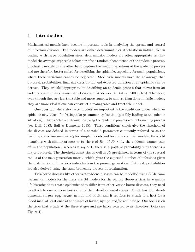
the ticks that attach at the three stages and are hence referred to as three-host ticks (see

Figure 1).

3

Figure 1: The developmental stages in the life cycle of a three-host tick.

It is during the attachment that a tick may transmit the disease if infected and is

attached to a susceptible host, or it can get infected if susceptible and attached to an

infectious host. A simple way of describing the transmission dynamics would be to disregard

the stage structure of the tick as is done in Paper 1. On the other hand it is of interest

to find out if anything is gained by including the stage structure of the tick as is done in

Paper 2. A brief summary of both papers is now given below.

In the first paper, we define a stochastic model motivated by the deterministic model

developed by Mwambi (2002). We combine all the stages of the tick into one compartment

and only classify a tick according to its infectious state and whether or not it is attached

to a host, and the host population is categorised as susceptible, infected or recovered. The

model developed is a seven dimensional Markov process. For this model, a tick may attach

and detach several times before dying, and this will have an impact on the transmission

dynamics of the disease. Using a three-type branching process approximation, a threshold

parameter, which determines whether the epidemic may take off in the tick-cattle system,

is derived. The threshold parameter is shown to increase in the infection transmission rate

from host to tick, the transmission rate from tick to host, the tick attachment rate and the

tick birth rate. It decreases in the tick detachment rate, the tick mortality rate as well as in

the host mortality and recovery rates. The threshold parameter derived is reasonably similar

to the one obtained for the related deterministic model developed by Mwambi(2002) with

minor differences as a result of definition of some of the parameters. Outbreak probabilities

are computed using the branching process approximation and expressions for endemic level

4

in case of a major outbreak are derived. All results obtained are illustrated using numerical

examples and simulations. The outbreak probabilities as well as the infectious proportions

of the hosts and ticks at the endemic level increase as the threshold parameter increases.

In the second paper, a stochastic model that incorporates the stage structure of the

tick is formulated with an aim of developing a more realistic model than the one developed

in the first paper. The model is therefore an extension of the model developed in Paper

1 and is a fourteen dimensional Markov process. With the incorporation of the stage

structure, a tick can only attach three times and of this, it can get infected only at the

larvae and nymph stages and may infect a susceptible host only at the nymph and adult

stages. The transmission dynamics will therefore differ with those of the simpler model

in Paper 1. The threshold condition for the persistence of the disease, the probability of

a major outbreak and endemic level of the disease are derived. The threshold condition

is defined in terms of a threshold quantity which depends on the population dynamics

parameters of the tick-host system as well as the transmission parameters. It is shown that

the number of infectives in the tick-host system increase when the tick attachment rates

of the different stages of the tick, the transmission rates from host to larvae (nymph) and

the transmission rate from nymph (adult) to host increase; and decrease when the tick

detachment rates for the different stages of the tick increase. A threshold quantity similar

to the one derived in this paper is obtained using a deterministic model by Rosa et al.

(2007). A comparison of a ”homogeneous version” of the more complicated model and the

one stage model is done. The two models (one stage and homogeneous version) are made

as similar as possible through calibration of their model parameters. It is shown that the

two models are genuinely different with the homogenous version having smaller threshold

quantity and lower outbreak probabilities. The reason for this is that an infected tick in

the stage structured model infects fewer susceptible hosts (at most two) than in the one

stage model. These results are illustrated using numerical examples and simulations.

5

References

ANDERSSON, H & BRITTON, T. (2000) Stochastic epidemic models and their statistical

analysis. Springer Lecture Notes in Statistics vol.151. New York: Springer-Verlag

BALL, F. (1983): The threshold behaviour of epidemic models. J Appl. Prob, 20, 227-242.

BALL, F. & DONNELLY, P. (1995) Strong approximations for epidemic models. Stoch.

Proc. Appl., 55, 1-21.

MWAMBI, H. (2002) Ticks and tick borne diseases in Africa: a disease transmission model.

IMA J. Math. Appl. Med. Biol., 19, 275-292.

ROSA,R., PUGLIESE,A. (2007) Effects of tick population dynamics and host densities on

the persistence of tick-borne infections. Math. Biosci., 208, 216-240.

6

A Stochastic epidemic model for tick borne diseases:

Initial stages of an outbreak and endemic levels

ANNE WANGOMBE∗†, MIKAEL ANDERSSON‡, TOM BRITTON§

Department of Mathematics, Stockholm University, SE-10691 Stockholm, Sweden

A stochastic model describing the disease dynamics for a tick borne disease amongst

cattle is developed. The spread of the disease at its initial stages is approximated by a

three-type branching process assuming that the initial sub-populations of susceptible ticks

(attached and detached) and cattle are large; while those of the infected ticks and cattle

are small. Using this approximation, a threshold condition which determines whether the

epidemic may take off in the tick-cattle system is derived. This condition expressed as

a threshold parameter, is shown to increase in the infection transmission rates, the tick

attachment rate and the tick birth rate. It decreases in the tick detachment rate, the tick

mortality rate as well as in the host mortality and recovery rates. Outbreak probabilities

and endemic levels in case of a major outbreak are also calculated.

Keywords : deterministic system; disease persistence; endemic level; multi-type branching

process; threshold parameter; tick-borne diseases

1 Introduction

Tick borne diseases affecting cattle pose major health and management problems in Sub

Saharan Africa (Norval et al., 1992; Latif, 1993). The prevalence of these diseases have

therefore been given considerable attention in an attempt to find ways of managing and

controlling them (International Livestock Research Institute website,www.ilri.org). The

tick borne diseases affecting cattle in this region include heartwater caused by Cowdria

ruminantium and spread by the tick vector Amblyomma hebraeum, babesiosis caused by

babesia bigemina and spread by the tick vector Boophilus microplus and East Coast Fever

caused by Theileria parva and spread by the tick vector Rhicephalus appendiculatus, also∗E-mail: wachiraanne@hotmail.com†Permanent adress: School of Mathematics, University of Nairobi, P.O Box 30197-00100, Nairobi.‡E-mail: mikaela@math.su.se§E-mail: tomb@math.su.se

1

known as the brown ear tick. Of these diseases, heartwater and East Coast Fever lead

to huge economic losses through appreciable mortality and morbidity, and also through

reduction in growth rates and productivity of recovered cattle (Young et al., 1988; ICIPE,

2005). The biology and epidemiology of Theileria parva and Cowdria ruminatium have

been reviewed by several authors, Norval et al. (1992); Medley (1994); O’Callaghan et al.

(1998); Mc Dermott et al. (2000) and Makala et al. (2003) among others. The problem

of transmission dynamics of these parasites in endemically stable environments have been

studied mathematically by Medley et al. (1993); Norval et al. (1992)and Mwambi(2002) .

Most models developed for tick borne diseases are deterministic. Although these models

have contributed much to the understanding of the biological processes which underlie the

spread of disease, the importance of random effects in determining population dynamic

patterns of disease incidence and persistence is not reflected. One question where stochas-

tic models are important is the conditions under which the epidemic process may become

endemic depending on its spread at the early stages. Another problem is the probability

of a major outbreak occurring, i.e that an epidemic takes off in a population. Stochastic

models are also appropriate in describing an epidemic process that moves from an endemic

state to the disease extinction state (Andersson & Britton, 2000, ch 8). Therefore they are

more ideal if one can construct a manageable and tractable model.

Mwambi (2002) developed a deterministic transmission model for tick borne disease for

cattle. The model is a seven dimensional system of ordinary differential equations in which

he combined the larvae, nymph and adult stages of the tick into one compartment and as-

sumed a constant host density per unit area. He investigated conditions for the persistence

of a steady tick population. He also derived a threshold quantity for the disease which is

dependent on the host density, the parameters of the tick-cattle interaction system and the

two disease transmission rates from tick vector to cattle host and vice versa.

In the present paper we define a stochastic model related to the deterministic model de-

veloped by Mwambi and derive properties of it. However, in the model developed in this

paper, functions of some parameters differ in definition from those in the deterministic

model. These differences are mentioned in the discussion when we make comparisons of the

threshold quantities derived in both models.

One of the main results of the study is the derivation of the necessary condition for the

possibility of a major outbreak in the tick-cattle system when randomness is taken into

account, given that the disease is introduced when the susceptible tick and cattle popula-

tions are in equilibrium. This condition is formulated in terms of a threshold parameter

which depends on the parameters governing the tick-cattle system as well as the infection

transmission rates of both the ticks and the cattle. A consequence of this result is the

2

possibility of attaining an endemic equilibrium state in the system when the threshold pa-

rameter is larger than one. Another main result is the derivation of the probability of an

outbreak occurring (leading to endemicity) under the same conditions. This is achieved by

a branching process approximation.

The paper is structured as follows: In Section 2, the stochastic model for the tick and cattle

populations and epidemic is described in detail. In Section 3, a three-type branching pro-

cess is used to approximate the initial stages of the epidemic process. This approximation

is used to derive threshold conditions for the possibility of the disease becoming endemic.

In Section 4, expressions for the probability of a major outbreak under different circum-

stances are derived. In Section 5, we derive an endemic equilibrium using the embedded

deterministic system of the stochastic model defined in Section 2. In Section 6, the main

results are examined using numerical examples and simulations. Finally in Section 7, we

give a brief discussion on the study, its limitations as well as suggestions for possible further

work.

2 A stochastic model for tick borne disease

Motivated by the deterministic model developed by Mwambi (2002), we now define a model

which is a stochastic version of the deterministic model. In the model, the individuals

in the host (cattle) population are categorised as Susceptible (HS), Infectious (HI) and

Recovered (HR). The individuals in the tick population are categorised as: detached and

infectious (DI); detached and susceptible (DS); attached and infectious (AI) and attached

and susceptible (AS). These categories of the tick vector depend on a tick’s infection status

as well as whether it is attached to a host or not. Once a tick get infected it remains

infectious until it dies.

2.1 Model definition

2.1.1 Host population dynamics without ticks and disease

For the model, we want the size of the host population H(t)(per unit area) to fluctuate

around a constant value, N ; i.e H(t) = HS(t) + HI(t) + HR(t) ≈ N at any time t. This

is obtained by having a constant birth rate µN , and each host having an exponential life-

length with death rate µ.

3

2.1.2 Tick-host interaction system without the disease

The host population is not affected by susceptible ticks and therefore its dynamics remain

as mentioned in the previous section.

For the tick population, ticks require a blood meal from a host in order to develop fully

and for females to reproduce. Since, in nature, adult female ticks lay eggs after detaching,

we could let the number of newborn ticks depend on the number of newly detached ticks.

However, since it is not easy to keep track of the number of newly detached ticks (and this

also ruins the Markovian property of the model), the birth rate of ticks is defined to be

proportional to the total number of attached ticks A(t); (A(t) = AS(t) + AI(t)); as it is

roughly proportional to the number of newly detached ticks. An individual tick gives birth

at the rate ρ, hence new ticks are born at the rate ρA(t).

The attachment rate of a tick is treated as a decreasing function of the total number of

attached ticks A(t) in the system and an increasing function of the host population H(t).

We have chosen the functional relationship, αH(t)1+A(t)

, as the attachment rate of a detached

tick. The constant 1 is added to A(t) in the denominator so that if the number of attached

ticks is zero then the overall attachment rate of a tick will be αH(t) rather than infinity.

For large populations (which we assume in the study) the effect of the constant is neglible,

i.e αH(t)1+A(t) ' α

H(t)A(t) . The overall attachment rate is αH(t)

1+A(t)D(t), where D(t) = DS(t)+DI(t).

An attached tick detaches at the rate δ, hence the overall detachment rate is δA(t).

Tick mortality is considered only for detached ticks which die at rate ν independent of

everything else. The mortality rate of ticks is hence νD(t).

2.1.3 Host-tick-disease interaction system

Both ticks and hosts transmit the parasite that causes the disease. While infectious, a host

infects each susceptible tick attached to it at rate β, so the overall infection transmission

rate from hosts to ticks is βHI(t)AS(t)

N . The infectious hosts may either recover from the

disease at the rate γ, hence γHI(t) is the overall recovery rate; or die at the rate µ, hence

µHI(t) is the death rate. Recovered hosts are considered immune to the disease but ticks

may still attach to them. A recovered host dies at the rate µ, hence the overall death rate

is µHR(t).

While attached to susceptible hosts, infectious attached ticks may infect their host at the

rate σ, so the overall infection transmission rate from ticks to hosts is σAI(t)HS(t)

N .

The stochastic model for the process

(DS(t), DI(t), AS(t), AI(t), HS(t), HI(t), HR(t), t > 0) is summarised in Table 1, (having

initial values (DS(0), DI(0), AS(0), AI(0), HS(0), HI(0), HR(0))). It is a seven dimensional,

4

integer-valued Markov process with respective jump intensities as illustrated in Fig. 1.

In the model defined we have made the simplification that susceptible attached ticks get

infected at a rate proportional to the total number of infectious hosts. This means that the

infection status of the actual host the tick is attached to is irrelevant. Another simplification

is that the attachment rate is proportional to the total number of attached ticks in the

system and not the number of attached ticks on a particular host that a tick wants to attach

to. We have also assumed that the host and tick populations mix uniformly implying that

any tick has an equal chance of attaching to any host in the system. Further, we have

assumed no increased death rate of host or tick population due to the disease. Finally we

have assumed that there are no seasonal effects in the system.

Table 1: Stochastic model for tick-host-disease system starting from (DS , DI , AS , AI, HS, HI, HR).

to transition rate event

→ (DS + 1, DI , AS, AI , HS, HI , HR) ρA birth of a susceptible tick

→ (DS − 1, DI , AS + 1, AI , HS, HI , HR) αH1+ADS attachment of a susceptible

detached tick

→ (DS + 1, DI , AS − 1, AI , HS, HI , HR) δAS detachment of a susceptible

attached tick

→ (DS − 1, DI , AS, AI , HS, HI , HR) νDS death of a susceptible detached

tick

→ (DS , DI − 1, AS, AI + 1, HS, HI , HR) αH1+ADI attachment of an infectious

detached tick

→ (DS , DI + 1, AS, AI − 1, HS, HI , HR) δAI detachment of an infectious

attached tick

→ (DS , DI − 1, AS, AI , HS, HI , HR) νDI death of an infectious detached

tick

→ (DS , DI, AS − 1, AI + 1, HS, HI , HR) βHIASN infection of a suceptible

attached tick

→ (DS , DI, AS , AI , HS − 1, HI + 1, HR) σAIHSN infection of a susceptible host

→ (DS , DI, AS , AI , HS + 1, HI , HR) µN birth of a susceptible host

→ (DS , DI, AS , AI , HS − 1, HI , HR) µHS death of a susceptible host

→ (DS , DI, AS , AI , HS , HI − 1, HR) µHI death of an infectious host

→ (DS , DI, AS , AI , HS , HI − 1, HR + 1) γHI recovery of an infectious host

→ (DS , DI, AS , AI , HS , HI , HR − 1) µHR death of a recovered host

5

Figure 1: Schematic representation of the model.

2.2 Disease free tick-host subsystem

One of the sub-systems that is of interest is that of a disease-free population, where all

individuals are susceptible. This sub-system is a Markov process with jump intensities as

defined in Table 2. We now derive the disease free tick-host system (HS , AS , DS), where all

states have equal rates of entering and leaving the state. Given that the host population is

Table 2: Stochastic model for uninfected subsystem.

to transition rate Event

(DS , AS, HS) → (DS + 1, AS − 1, HS) δAS detachment of tick

(DS , AS, HS) → (DS − 1, AS + 1, HS) αHS1+AS

DS attachment of tick

(DS , AS, HS) → (DS + 1, AS , HS) ρAS birth of tick

(DS , AS, HS) → (DS − 1, AS , HS) νDS death of tick

(DS , AS, HS) → (DS , AS, HS + 1) µN birth of host

(DS , AS, HS) → (DS , AS, HS − 1) µHS death of host

in equilibrium;

µN = µHS(t)

and hence

HS = N, (1)

6

then for the subsystem to attain a steady state the tick vector population should be in

equilibrium. At equilibrium, the birth and death rates of ticks are equal as well as the

detachment and attachment rates. Thus,

ρAS(t) = νDS(t)αHS(t)

1 + AS(t)DS(t) = δAS(t).

By solving the two equations we obtain,

AS =αρHS

δν− 1 =

αρN

δν− 1 ≈ αρN

δν(2)

DS =ρAS

ν=

αρ2N

δν2− ρ

ν≈ αρ2N

δν2=

ρ

νAS (3)

HS , AS and DS are the population sizes of susceptible hosts, susceptible attached ticks and

susceptible detached ticks in the disease free equilibrium.

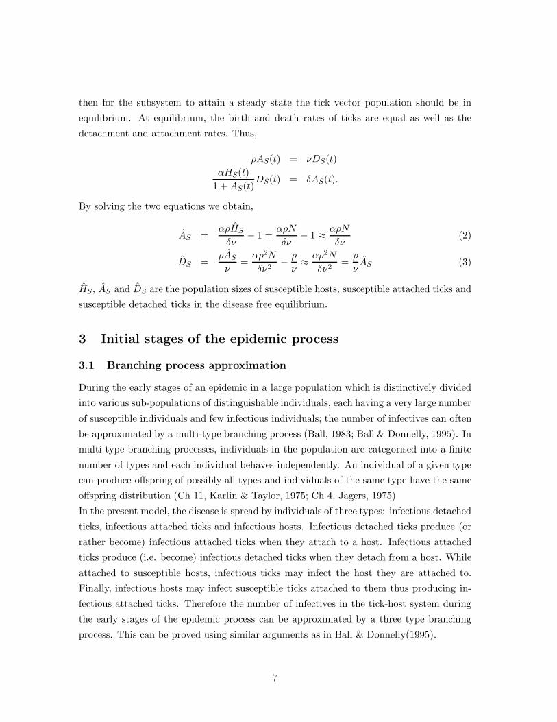
3 Initial stages of the epidemic process

3.1 Branching process approximation

During the early stages of an epidemic in a large population which is distinctively divided

into various sub-populations of distinguishable individuals, each having a very large number

of susceptible individuals and few infectious individuals; the number of infectives can often

be approximated by a multi-type branching process (Ball, 1983; Ball & Donnelly, 1995). In

multi-type branching processes, individuals in the population are categorised into a finite

number of types and each individual behaves independently. An individual of a given type

can produce offspring of possibly all types and individuals of the same type have the same

offspring distribution (Ch 11, Karlin & Taylor, 1975; Ch 4, Jagers, 1975)

In the present model, the disease is spread by individuals of three types: infectious detached

ticks, infectious attached ticks and infectious hosts. Infectious detached ticks produce (or

rather become) infectious attached ticks when they attach to a host. Infectious attached

ticks produce (i.e. become) infectious detached ticks when they detach from a host. While

attached to susceptible hosts, infectious ticks may infect the host they are attached to.

Finally, infectious hosts may infect susceptible ticks attached to them thus producing in-

fectious attached ticks. Therefore the number of infectives in the tick-host system during

the early stages of the epidemic process can be approximated by a three type branching

process. This can be proved using similar arguments as in Ball & Donnelly(1995).

7

3.2 Threshold condition for disease outbreak

Let N , the average population size of hosts, be sufficiently large and assume that the tick

and host populations are in equlibrium before the disease is introduced in the system.

During the early stages of the epidemic the population sizes of the susceptible ticks and

hosts are very large compared to the population sizes of the infectious ticks and hosts. As

a consequence the attachment rate of a tick is approximately,

αH(t)1 + A(t)

' αN

A=

δν

ρ

where H(t) and A(t) are the total host population and the number of attached ticks at

time t; and A (A = AS) is the total number of attached ticks in equilibrium state (given in

Equation 2).

Suppose the disease is introduced by a few infectious hosts and/or infectious ticks, then

the infectious detached ticks, infectious attached ticks and infectious hosts will spread the

disease. Let the infectious detached ticks be of type 1, infectious attached ticks be of type 2

and infectious hosts be of type 3. Further let {Xij ; i, j = 1, 2, 3} be the number of infectives

of type j produced by an infective of type i and mij = E [Xij ]. We now derive the offspring

distributions and its expected values for the approximating branching process.

Beginning with the infectious detached ticks; an infectious detached tick produces at most

one single infectious attached tick but no other offspring, hence X11 ≡ X13 ≡ 0.

While on the ground, an infectious detached tick either dies at rate ν or it attaches to a

host at rate αNA

and becomes an infectious attached tick; so

P (X12 = 0) =ν

ν + αNA

=νA

νA + αN,

P (X12 = 1) =αN

νA + αN.

The expected numbers of infectious detached ticks, infectious attached ticks and infectious

hosts produced by one infectious detached tick are hence

m11 = E [X11] = 0,

m12 = E [X12] =αN

νA + αN,

m13 = E [X13] = 0.

Next, an infectious attached tick detaches producing a detached infectious tick with cer-

tainty, so X21 ≡ 1. An infectious attached tick does not produce another infectious attached

tick, hence X22 = 0. Finally an infectious attached tick (one that is attached to a suscep-

tible host) produces at most one infectious host. Since nearly all hosts are susceptible in

8

the early stages of the epidemic process, the probability that an infectious tick is attached

to a susceptible host during this period is approximately one(

HS(t)N ' 1

). An infectious

tick is attached to a susceptible host for a time duration which is exponentially distributed

with intensity δ (δ is the detachment rate), and it infects the susceptible host at the rate σ

before detaching. Thus

P (X23 = 0) =δ

δ + σ,

P (X23 = 1) =σ

δ + σ.

The expected numbers of infectious detached ticks, infectious attached ticks and infectious

hosts produced by one infectious attached tick are hence

m21 = E [X21] = 1,

m22 = E [X22] = 0,

m23 = E [X23] =σ

δ + σ.

Finally, for the infectious hosts; an infectious host can only produce infectious attached

ticks, hence X31 ≡ X33 ≡ 0. A host is infectious for a time period that is exponentially

distributed with intensity µ + γ (it either dies at the rate µ or it recovers at the rate γ).

During this period it infects susceptible ticks attached to it according to a Poisson process

with intensity β AN ; since AS

N = AN at the initial stages of the epidemic process. Here we

make the simplifying assumption that the number of susceptible attached ticks remains

fairly constant throughout the infectious period.

Conditioning on I , the length of the infectious period, the expected number of susceptible

ticks that get infected before this period ends is

E [X32] = E (E[X32|I ]) = E

(β

A

NI

)

= βA

NE[I ] =

β AN

µ + γ

=βA

N(µ + γ).

The expected numbers of infectious detached ticks, infectious attached ticks and infectious

hosts produced by one infectious host are hence

m31 = E [X31] = 0,

m32 = E [X32] =βA

N(µ + γ),

m33 = E [X33] = 0.

9

Let M = {mij}3i,j=1 be the expectation matrix of the form

M =

0 αNαN+νA

0

1 0 σσ+δ

0 βAN(µ+γ) 0

.

If the largest real-valued eigenvalue of M is less than or equal to one, the epidemic dies out

fairly quickly. On the other hand, if the largest real-valued eigenvalue of M is greater than

one, then there is a positive probability that the epidemic takes off (Karlin& Taylor, 1975,

p. 412).

The eigenvalues of M are the roots of the characteristic equation

λ3 − λ

(βA

N(µ + γ)σ

σ + δ+

αN

αN + νA

)= 0. (4)

From Equation(4), the largest eigenvalue is the positive root of the expression

λ2 =βσA(αN + νA) + αN2(µ + γ)(σ + δ)

N(αN + νA)(µ + γ)(σ + δ).

Since we are interested in the case where the largest eigenvalue is greater than one, then

λ > 1 implies that λ2 > 1.

Thus for λ to be greater than 1, then we must have that

βσA(αN + νA) + αN2(µ + γ)(σ + δ) > N(αN + νA)(µ + γ)(σ + δ),

This expression reduces to

βσ(αN + νA)Nν(σ + δ)(µ + γ)

> 1. (5)

Using Equation(2), the value of A will be

A = AS ' Nαρ

δν

since we assume that all susceptible sub-populations are sufficiently large.

Substituting for A in Equation(5), we obtain

T =βσα

(1 + ρ

δ

)

ν(σ + δ)(µ + γ). (6)

T is the threshold quantity when the tick-host system is in equilibrium at the time of disease

introduction. From Equation(6) we see that T has a monotonic dependence on all the eight

model parameters. It decreases in the tick detachment rate δ, host birth and mortality rate

10

µ, tick mortality rate ν and host recovery rate γ. It increases in the tick-host encounter

rate α, the infection transmission rate from tick to host σ, the infection transmission rate

from host to tick β as well as the tick birth rate ρ. When T ≤ 1, the epidemic dies out

fairly quickly and when T > 1, the epidemic may take off in the system and has a chance

of becoming endemic.

4 The probability of a major outbreak

Let the probability generating function of the offspring distribution of infectives produced

by an infective of type i (i = 1, 2, 3), be Gi(s) = E[∏3

j=1 sXij

j

], where Xij is as defined

in the previous section and s = (s1, s2, s3) . The probability that a minor outbreak of

the disease occurs given that there are ai infectives initially of each of the three types is

π = πa11 πa2

2 πa33 . Since M is irreducible, we know that π1 = π2 = π3 = 1 if T ≤ 1 or that

φ = (π1, π2, π3) is the unique root of s = G(s) that satisfies π1 < 1, π2 < 1 and π3 < 1 if

T > 1.

Since X11 ≡ X13 ≡ 0 and X12 equals zero or one, the probability generating function

of offspring produced by one infectious detached tick is

G1(s) = E[sX111 sX12

2 sX133

]= P (X12 = 0)s0

2 + P (X12 = 1)s12

=νA

αN + νA+

αN

αN + νAs2.

Since X21 ≡ 1, X22 ≡ 0 and X23 equals zero or one, the probability generating function of

offspring produced by one infectious attached tick is

G2(s) = E[sX211 sX22

2 sX233

]= s1

1

[P (X23 = 0)s0

3 + P (X23 = 1)s13

]

=(

δ

σ + δ+

σ

σ + δs3

)s1.

Since X31 ≡ X33 ≡ 0 and X32 is Poisson distributed conditioned on that the infectious

period I = t (as explained in the previous section), the probability generating function of

offspring produced by one infectious host is

11

G3(s) = E[sX211 sX22

2 sX233

]=∑

x

sx2P (X32 = x)

=∑

x

sx2

∫ ∞

0

(µ + γ)e−(µ+γ)te

(β A

Nt) (

β AN t)x

x!dt

=∫ ∞

0

(µ + γ)e−(µ+γ+β AN

)t

∞∑

x=0

sx2

(β A

N t)x

x!

dt

=∫ ∞

0

(µ + γ)e−(µ+γ+β AN

)teβ AN

ts2dt

= (µ + γ)∫ ∞

0e−(µ+γ+β A

N−β A

Ns2)tdt

=N(µ + γ)

N(µ + γ) + βA − βAs2

.

Substituting A = Nραδν ; the non-trivial solutions s1, s2 and s3 for the equations si =

Gi(s), i = 1, 2, 3 can be shown to satisfy

s1 =(σ + δ)[βαρ(δ + ρ) + δ2ν(µ + γ)]

βα(ρ + δ)[σ(ρ + δ) + ρδ](7)

s2 =δ[ν(µ + γ)(δ + σ) + βαρ]

βα[ρδ + σ(δ + ρ)](8)

s3 =(µ + γ)δν[σ(δ + ρ) + ρδ]

σ[βαρ(δ + ρ) + δ2ν(µ + γ)](9)

and extinction probabilities are given by πi=min(1, si). The analytical solution in this case

can be derived which is not common for multi-type branching processes.

In Section 6, π1,π2,π3 and (1 − π) are computed numerically for some examples.

5 Endemic level of the epidemic process

Assume that the tick-host system is in equilibrium before the disease is introduced. The

threshold value T defined in (6) is useful in determining the possibility of the epidemic

taking off in the system. If T ≤ 1 then the epidemic will die out fairly quickly and the

tick-host system will attain a disease-free equilibrium state. On the other hand if T > 1,

then either a minor outbreak occurs where only few ticks and hosts get infected before the

infection disappears from the population; or else a major outbreak occurs and the disease

may become endemic (taking the host and tick populations to a substantial infection level

12

known as the endemic level). At this level, the tick-host system is said to be in an endemic

equilibrium state.

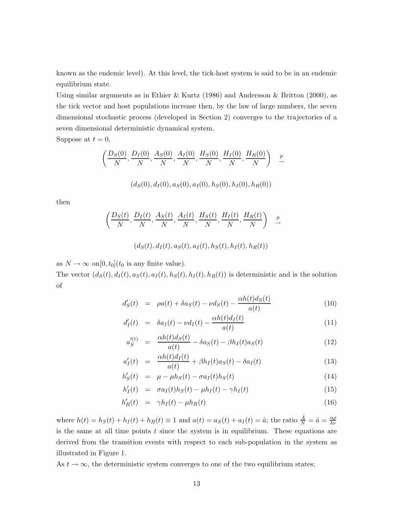
Using similar arguments as in Ethier & Kurtz (1986) and Andersson & Britton (2000), as

the tick vector and host populations increase then, by the law of large numbers, the seven

dimensional stochastic process (developed in Section 2) converges to the trajectories of a

seven dimensional deterministic dynamical system.

Suppose at t = 0,(

DS(0)N

,DI(0)

N,AS(0)

N,AI(0)

N,HS(0)

N,HI(0)

N,HR(0)

N

)p→

(dS(0), dI(0), aS(0), aI(0), hS(0), hI(0), hR(0))

then(

DS(t)N

,DI(t)

N,AS(t)

N,AI(t)

N,HS(t)

N,HI(t)

N,HR(t)

N

)p→

(dS(t), dI(t), aS(t), aI(t), hS(t), hI(t), hR(t))

as N → ∞ on[0, t0](t0 is any finite value).

The vector (dS(t), dI(t), aS(t), aI(t), hS(t), hI(t), hR(t)) is deterministic and is the solution

of

d′S(t) = ρa(t) + δaS(t) − νdS(t)− αh(t)dS(t)a(t)

(10)

d′I(t) = δaI(t)− νdI(t) −αh(t)dI(t)

a(t)(11)

a′(t)S =

αh(t)dS(t)a(t)

− δaS(t)− βhI(t)aS(t) (12)

a′I(t) =αh(t)dI(t)

a(t)+ βhI(t)aS(t) − δaI(t) (13)

h′S(t) = µ − µhS(t)− σaI(t)hS(t) (14)

h′I(t) = σaI(t)hS(t)− µhI(t) − γhI(t) (15)

h′R(t) = γhI(t) − µhR(t) (16)

where h(t) = hS(t) + hI(t) + hR(t) ≡ 1 and a(t) = aS(t) + aI(t) = a; the ratio AN = a = αρ

δν

is the same at all time points t since the system is in equilibrium. These equations are

derived from the transition events with respect to each sub-population in the system as

illustrated in Figure 1.

As t → ∞, the deterministic system converges to one of the two equilibrium states;

13

(i) The disease free equilibrium state if dI(0) = aI(0) = hI(0) = 0 or if dI(0) + aI(0) +

hI(0) > 0 and T ≤ 1

(ii) The endemic equilibrium state if dI(0) + aI(0) + hI(0) > 0 and T > 1.

Disease free equilibrium state:

This state can be attained in two ways:

(i) If the disease is not present in the system initially, i.e. dI(0) = aI(0) = hI(0) = 0,

then for dS(t), aS(t) and hS(t), the deterministic system is:

d′S(t) = (ρ + δ)aS(t) − αhS(t)dS(t)aS(t)

− νdS(t)

a′S(t) =αhS(t)dS(t)

aS(t)− δaS(t)

h′S(t) = µ(1 − hS(t))

The solution of this system of equations all equated to zero gives us;

dS =ρ2α

δν2, aS =

ρα

δν, hS = 1

corresponding to Equations (1-3).

(ii) If the disease is present initially in the system, i.e dI(0)+aI (0)+hI(0) > 0 and T ≤ 1,

then

[dI(t), aI(t), hI(t), hR(t)] → [0, 0, 0, 0]

and

dS(t) → dS =ρ2α

δν2, aS(t) → aS =

ρα

δν, hS(t) → hS = 1.

Therefore the disease free equilibrium state will have dI(t) = aI(t) = hI(t) = hR(t) =

0 and the proportions dS(t), aS(t) and hS(t) will converge to the values (dS , aS, hS).

Endemic equilibrium state:

When T > 1, then the tick-host system can converge to an endemic equilibrium state. If

this state is attained then it is the positive solution of the system of Equations (10-16)

having derivatives all equal to zero.

Using the values h = 1, a = αρδν and d = ρ2α

δν2 obtained for the disease free state, the solution

14

can be shown to satisfy:

dS =ρ2[σαρ (δ(ρ + δ)(µ + γ) + βµ(ρ + δ)) + δ3νµ(µ + γ)]

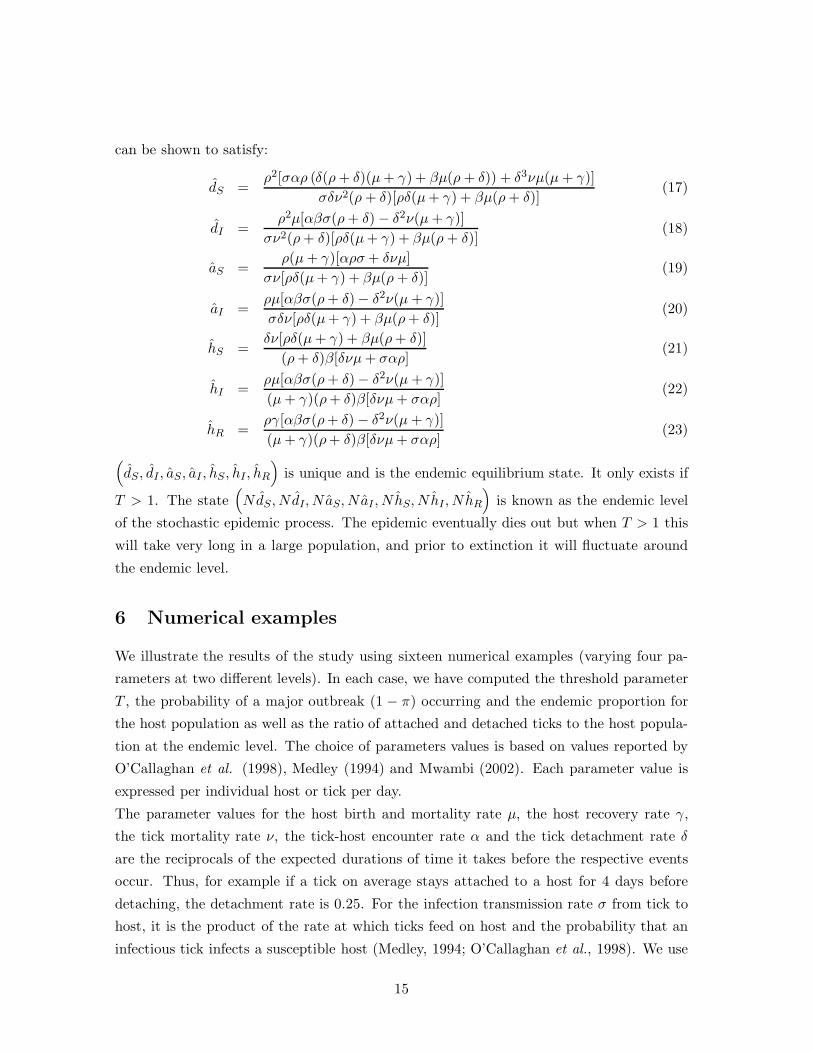
σδν2(ρ + δ)[ρδ(µ + γ) + βµ(ρ + δ)](17)

dI =ρ2µ[αβσ(ρ + δ) − δ2ν(µ + γ)]

σν2(ρ + δ)[ρδ(µ + γ) + βµ(ρ + δ)](18)

aS =ρ(µ + γ)[αρσ + δνµ]

σν[ρδ(µ + γ) + βµ(ρ + δ)](19)

aI =ρµ[αβσ(ρ + δ)− δ2ν(µ + γ)]σδν[ρδ(µ + γ) + βµ(ρ + δ)]

(20)

hS =δν[ρδ(µ + γ) + βµ(ρ + δ)]

(ρ + δ)β[δνµ + σαρ](21)

hI =ρµ[αβσ(ρ + δ)− δ2ν(µ + γ)](µ + γ)(ρ + δ)β[δνµ + σαρ]

(22)

hR =ργ[αβσ(ρ + δ) − δ2ν(µ + γ)](µ + γ)(ρ + δ)β[δνµ + σαρ]

(23)

(dS , dI , aS , aI , hS , hI , hR

)is unique and is the endemic equilibrium state. It only exists if

T > 1. The state(NdS , NdI, NaS, NaI , NhS, NhI , NhR

)is known as the endemic level

of the stochastic epidemic process. The epidemic eventually dies out but when T > 1 this

will take very long in a large population, and prior to extinction it will fluctuate around

the endemic level.

6 Numerical examples

We illustrate the results of the study using sixteen numerical examples (varying four pa-

rameters at two different levels). In each case, we have computed the threshold parameter

T , the probability of a major outbreak (1 − π) occurring and the endemic proportion for

the host population as well as the ratio of attached and detached ticks to the host popula-

tion at the endemic level. The choice of parameters values is based on values reported by

O’Callaghan et al. (1998), Medley (1994) and Mwambi (2002). Each parameter value is

expressed per individual host or tick per day.

The parameter values for the host birth and mortality rate µ, the host recovery rate γ,

the tick mortality rate ν, the tick-host encounter rate α and the tick detachment rate δ

are the reciprocals of the expected durations of time it takes before the respective events

occur. Thus, for example if a tick on average stays attached to a host for 4 days before

detaching, the detachment rate is 0.25. For the infection transmission rate σ from tick to

host, it is the product of the rate at which ticks feed on host and the probability that an

infectious tick infects a susceptible host (Medley, 1994; O’Callaghan et al., 1998). We use

15

similar arguments to estimate the infection transmission rate β from host to tick as the

product of the rate at which ticks feed on host and the probability that an infectious host

infects a susceptible attached tick. Finally, the tick birth rate ρ is the average number of

ticks produced per tick per day.

For α, β, δ and σ; we choose two values for each parameter; one high and one low value;

and combine these values to obtain sixteen possible cases. These parameters are considered

to be most influential in determining the infection dynamics in the tick-host-disease system

when both the host and tick populations are sufficiently large (Mwambi, 2002; O’Callaghan

et al., 1998). The other parameters are set to be fixed.

6.1 Threshold parameter T

The parameter values chosen are summarised in Table 3 as well as the threshold parameter T

obtained from Equation(6). From the values of T obtained for the sixteen cases considered,

we observe that increasing the value of δ, while holding all other parameters constant,

decreases T . On the other hand, increasing the value of each of the parameters α, β or

σ individually, while holding all other parameters constant, increases T . This result is

consistent with the monotonic dependencies observed earlier in Section 3. We also observe

that for most cases where T is larger than one (Cases 3,7,11,15); the parameter α has a

high value while δ has a low value. For cases where both the parameters β and σ have high

values, the disease has a possibility of spreading when the parameter α has a low value

(Case 13).

16

Table 3: Different parameter values for β, σ, α ,δ; and the corresponding threshold parameter T

with fixed values ν=0.01, ρ=0.05, µ=0.0006 and γ=0.05.

Case β σ α δ T

1 0.01 0.005 0.03 0.05 0.11

2 0.01 0.005 0.03 0.5 0.006

3 0.01 0.005 0.3 0.05 1.08

4 0.01 0.005 0.3 0.5 0.06

5 0.01 0.02 0.03 0.05 0.39

6 0.01 0.02 0.03 0.5 0.03

7 0.01 0.02 0.3 0.05 3.39

8 0.01 0.02 0.3 0.5 0.25

9 0.05 0.005 0.03 0.05 0.54

10 0.05 0.005 0.03 0.5 0.03

11 0.05 0.005 0.3 0.05 5.39

12 0.05 0.005 0.3 0.5 0.32

13 0.05 0.02 0.03 0.05 1.69

14 0.05 0.02 0.03 0.5 0.13

15 0.05 0.02 0.3 0.05 16.94

16 0.05 0.02 0.3 0.5 1.25

6.2 Probability of a major outbreak

Using Equations (7-9) and the properties presented in Section 4, we calculate the theoretical

probability (1−π) of a major outbreak occurring starting with only one infectious detached

tick, one infectious attached tick and one infectious host initially in the epidemic process.

Though it is not realistic for an epidemic to be introduced by only one infective for each

sub-population, similar results for the probability of a major outbreak occurring can be

obtained using a few infectives for each sub-population. For all cases in Table 3 where

T < 1, the probability of a major outbreak is zero. For the rest of the cases where the

threshold parameter T is larger than one, the results are presented in Table 4, (the cases

are ordered according to their threshold value T). The results show that this probability

increases as the threshold parameter T increases and that an outbreak is almost certain for

parameter values chosen for Case 15. We ran 1000 simulations for the epidemic process for

cases 7, 11 and 15 in Table 4 to obtain the fraction of major outbreaks occurring (1 − π)

and compared the result with the theoretical probability (1 − π) obtained for these cases;

17

the other cases 3, 13 and 16 were omitted since larger populations than those chosen for the

simulations are needed to avoid extinction of the disease in the near future event though

the branching process initially may increase. The infection-free tick-host system was in

equilibrium with 50 susceptible hosts, 1500 susceptible attached ticks and 7500 susceptible

detached ticks, and the disease was introduced in the system by one infective member

for each of the three subpopulations. Each simulation was run until either there were no

infectives in the system (extinction) or there were 20 infectives in the system. The choice of

20 is arbitrary but it is assumed that if the number of infectives reaches 20 the epidemic will

not go extinct. The probabilty of a major outbreak is estimated by the proportion of the

simulations that do not go extinct before reaching 20 infectives. The results are presented

in Table 4. The proportions obtained are in good agreement with those of the theoretical

probabilities.

Table 4: Values of the theoretical probability of a major outbreak and the probability of majoroutbreak for simulated values of cases 7,11 and 15.

Case T π1 π2 π3 (1 − π) (1− π)

3 1.08 0.994 0.988 0.933 0.084

16 1.25 0.944 0.938 0.845 0.252

13 1.69 0.909 0.818 0.649 0.517

7 3.39 0.843 0.687 0.350 0.797 0.754

11 5.39 0.932 0.864 0.199 0.840 0.810

15 16.94 0.791 0.582 0.075 0.965 0.954

6.3 Endemic level

Equations (16-21) are used for calculations of the endemic proportions for the host popu-

lation and the average number of ticks (attached and detached) per host at endemic level.

For cases in Table 3 where T < 1, there is no posssibility of a major outbreak occurring

hence no endemic proportions for the host population or average number of ticks per host

at endemic level can be obtained. For cases where T > 1, the results are summarised in

Tables 5 as hS , hI , hR, and in Table 6 as aS , aI , dS , dI .

From Table 5, we observe that the proportion of infectious hosts increases as the

threshold parameter T increases though the percentage is fairly constant ranging between

0.2% and 1.1% of the host population. The percentage of susceptible hosts on the other

hand seems to decrease rapidly from 84.4% to 4.3% as T increases. For Case 15 where a

major outbreak leading to endemicity is almost certain to occur, approximately 4% and 1%

18

Table 5: Theoretical and simulated values of the endemic proportion for host population where thethreshold parameter is above one.

Case T hS hS hI hI hR hR

3 1.08 0.844 0.002 0.154

16 1.25 0.769 0.003 0.228

13 1.69 0.427 0.007 0.566

7 3.39 0.211 0.223 0.009 0.002 0.780 0.775

11 5.39 0.172 0.176 0.010 0.004 0.818 0.820

15 16.94 0.043 0.041 0.011 0.007 0.946 0.952

of the hosts are susceptible and infective respectively, and the remaining 95% are immune

at the endemic level. This result is close to the one obtained by Medley(1994) where he

considered the endemic stability of the East Coast Fever disease in Eastern Africa.

Table 6: Theoretical and simulated values of the average number of attached ticks and detachedticks per host for cases where the threshold parameter is above one.

Case T aS aS aI aI dS dS dI dI

3 1.08 29.98 0.02 149.94 0.06

16 1.25 2.99 0.01 14.96 0.04

13 1.69 2.96 0.04 14.90 0.10

7 3.39 29.89 29.96 0.11 0.05 149.72 149.82 0.28 0.21

11 5.39 29.42 29.43 0.58 0.57 148.60 148.75 1.40 1.27

15 16.94 29.33 29.38 0.67 0.63 148.30 148.52 1.70 1.50

From Table 6, we observe that the average number of infectious ticks (attached and

detached) per host increases as the threshold parameter T increases. For the attached

ticks, the average number increases more than thirty fold from 0.02 to 0.67 and that of the

detached ticks increases with an almost thirty fold from 0.06 to 1.7. The average number

of susceptible attached and detached ticks per host remain fairly constant.

No simulations were carried out for cases 3, 13 and 16 where T is slightly above one as the

endemic levels are too close to disease extinction because the population sizes chosen are

small. For cases 7, 11 and 15, one simulation for each case was carried out for a duration of

three years, beginning the process at the endemic level and the results were compared with

the numerical solutions obtained. For each simulation, the first year was disregarded and

the time averages of the remaining duration were used to obtain the endemic proportion of

19

the host population and the average number of ticks (attached and detached) per host at

the endemic level. The results are presented in Tables 5 and 6. The simulated values are

all relatively close to those of the numerical solutions for each of the subpopulations of the

susceptible and the infective hosts and ticks.

To illstrate the full distribution of the different states, we have plotted histograms of case

15 in Figs 2-4.

The results show that the endemic level of the susceptible hosts varies between 0 and

0 1 2 30

0.2

0.4

0.6

0.8

Number of susceptible hosts

rela

tive

fre

qu

en

cy

0 1 20

0.2

0.4

0.6

0.8

Number of infectious hosts

rela

tive

fre

qu

en

cy

43 44 45 46 470

0.2

0.4

0.6

0.8

Number of recovered hosts

rela

tive

fre

qu

en

cy

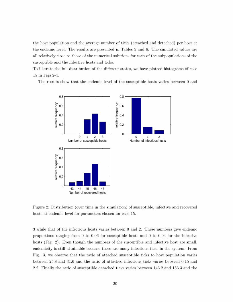
Figure 2: Distribution (over time in the simulation) of susceptible, infective and recovered

hosts at endemic level for parameters chosen for case 15.

3 while that of the infectious hosts varies between 0 and 2. These numbers give endemic

proportions ranging from 0 to 0.06 for susceptible hosts and 0 to 0.04 for the infective

hosts (Fig. 2). Even though the numbers of the susceptible and infective host are small,

endemicity is still attainable because there are many infectious ticks in the system. From

Fig. 3, we observe that the ratio of attached susceptible ticks to host population varies

between 25.8 and 31.6 and the ratio of attached infectious ticks varies between 0.15 and

2.2. Finally the ratio of susceptible detached ticks varies between 143.2 and 153.3 and the

20

24 26 28 30 320

0.002

0.004

0.006

0.008

0.01

0.012

0.014

Ratio of attached susceptible ticks to hosts

relat

ive fr

eque

ncy

0 1 2 30

0.02

0.04

0.06

0.08

0.1

0.12

Ratio of attached infectious ticks to hosts

Figure 3: Distribution (over time in the simulation) of the number of attached susceptible

and infective ticks per host at endemic level for parameters chosen for case 15.

140 145 150 1550

1

2

3

4

5

6

7

8x 10

−3

Ratio of detached susceptible ticks to hosts

relat

ive fr

eque

ncy

0 1 2 3 40

0.005

0.01

0.015

0.02

0.025

0.03

0.035

0.04

0.045

0.05

Ratio of detached infectious ticks to hosts

relat

ive fr

eque

ncy

Figure 4: Distribution (over time in the simulation) of the number of attached susceptible

and infective ticks per host at endemic level for parameters chosen for case 15.

21

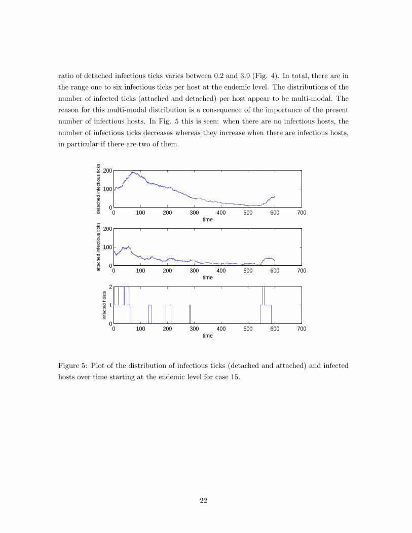
ratio of detached infectious ticks varies between 0.2 and 3.9 (Fig. 4). In total, there are in

the range one to six infectious ticks per host at the endemic level. The distributions of the

number of infected ticks (attached and detached) per host appear to be multi-modal. The

reason for this multi-modal distribution is a consequence of the importance of the present

number of infectious hosts. In Fig. 5 this is seen: when there are no infectious hosts, the

number of infectious ticks decreases whereas they increase when there are infectious hosts,

in particular if there are two of them.

0 100 200 300 400 500 600 7000

100

200

time

de

tach

ed

infe

ctio

us

ticks

0 100 200 300 400 500 600 7000

100

200

time

att

ach

ed

infe

ctio

us

ticks

0 100 200 300 400 500 600 7000

1

2

time

infe

cte

d h

ost

s

Figure 5: Plot of the distribution of infectious ticks (detached and attached) and infected

hosts over time starting at the endemic level for case 15.

22

7 Discussion

In this paper, we have developed a stochastic epidemic model for tick-borne diseases and

considered the threshold properties for the persistence of the disease, the probability of an

epidemic occurring and the endemic levels of the disease.

We observed that the necessary condition for the persistence of the disease, if it is intro-

duced when the tick-host interaction system is in equilibrium, depends on the parameters

governing the population dynamics of the system as well as the infection transmission be-

tween ticks and hosts, Equation(6). The effect of these parameters on the persistence of

the disease can therefore be determined. From numerical examples in Section 6, we ob-

serve how the parameters that are considered most influential in determining the disease

transmission dynamics affect the tick-host-disease system. An increase in the values of the

two infection transmission rates and/or the tick-host encounter rate (and consequently the

tick attachment rate) lead to an increase in the number of infectives while an increase of

the value of the tick detachment rate leads to a decrease in the number of infectives at the

endemic level. With reliable data for various parameter values in the model, Equation(6)

can be a useful tool in application to disease control strategies with efforts focused on re-

ducing parameters that enhance the spread of the epidemic and simultaneously increasing

parameters that reduce the spread. One way of achieving this is by making hosts resistant

to tick infestation (Mwambi, 2002) as well as vaccination (O’Callaghan et al.,1999).

The threshold parameter derived is reasonably similar to the one obtained for the related

deterministic model developed by Mwambi(2002). Both thresholds are increasing in the

attachment rate, tick birth rate, and the infection transmission rates. They both decrease

in tick mortality rate for detached ticks, host recovery rate, host mortality rate and tick de-

tachment rate. One difference in the two quantities is that the threshold quantity obtained

by Mwambi depends on parameters governing the tick-host-disease system as well as the

host density whereas the one we obtain depends only on the parameters governing the tick-

host-disease system. The reason that the threshold obtained in this study does not depend

on host density is that we define the tick-host ratio in terms of the parameters governing

the disease free tick-host interaction system (Section 2.2). The other difference is in the

choice of functions of the tick detachment rate and tick mortality rate for attached ticks.

Mwambi (2002) considers the tick detachment rate as an increasing function of the host

population whereas in our model it is independent of the host population. The detachment

of an attached tick occurs when it has had a complete blood meal or when it falls off the

host due to reasons (like the host shaking it off) not dependent on whether there are other

23

hosts to attach onto, hence we consider detachement to be independent of host population.

The tick mortality rate for attached ticks is incorporated in the deterministic model defined

by Mwambi but in our model we disregard it. Most literature on epidemic modelling for

tick borne diseases (O’Callaghan et al. (1998), Gilbert et al., (2001) and Rosa et al., (2007)

among others) do not cite mortality of ticks while attached to hosts, therefore we did not

include it in our model.

One advantage of stochastic models is that the probability that an epidemic (major out-

break) occurs can be derived. In our model we have shown that this probability can be

obtained from the parameters governing the tick-host-disease system. From Section 6, we

see that reducing T also reduces the probability of a major outbreak, hence any measures

taken to reduce T simultaneously reduces (1 − π). This result can not be obtained from

determinstic models which simply state with certainity that either an epidemic occurs or

it does not.

The model developed here has some limitations which should be addressed in order to for

it to be more accurate in modelling the tick-host system as well as making it more useful in

its application to control and intervention strategies. One limitation is the simplification of

the stage structure of the tick vector. In reality, the tick vector goes through four different

stages in its life cycle which in our model we have grouped into one compartment. However

as noted in Perry et al. (1993) and O’Callaghan et al. (1998), each developmental stage

has different effects on the tick-host interaction system as well as the disease transmission

dynamics. Another limitation is in the role of recovered hosts. We have assumed that

recovered cattle become immune and play no further role in the spread of the disease. In

reality, most of these animals may get infected again (secondary infection) and become

carriers of the disease. Susceptible ticks attaching to them may get infected and since they

remain infectious for long periods of time, the disease may persist for a long time leading to

an endemic state (Medley, 1994). Another limitation is that the infectious periods and life

durations are assumed to be exponentially distributed. Lastly, we model the attachment

rate as a decreasing function of the overall number of attached ticks rather than the actual

number on the host in question.

The limitations not withstanding, we believe our results are a first step towards more real-

istic stochastic modelling of tick borne diseases.

Acknowledgement

Anne Wangombe is grateful to the International Science Programme(ISP) at Uppsala Uni-

versity, Sweden, for financial support.

24

References

ANDERSSON, H & BRITTON, T. (2000) Stochastic epidemic models and their statistical

analysis. Springer Lecture Notes in Statistics vol.151. New York:Springer-Verlag

BALL, F.(1983): The threshold behaviour of epidemic models. J Appl. Prob, 20, 227-242.

BALL, F. & DONNELLY, P. (1995) Strong approximations for epidemic models. Stochas-

tic processes and their applications, 55, 1-21.

BRYAN, J., BROWN, C. & VIEIRA, A. (2004) Ticks and Animal Diseases. International

Vet. Med. Internet training module, College of Vet. Med., Univ. of Georgia.

ETHIER, S. & KURTZ, T.G. (1986) Markov processes: Characterisation and Convergence.

New York: Wiley & Sons

GILBERT, L., NORMAN, R., LAURENSON, M., REID, H. & HUDSON,P. (2001) Disease

persistence and apparent competition in a three host community: an empirical analytical

study of large scale wild populations. J. Anim. Ecol., 70, 1053-1061.

ICIPE (2005) Ticks and tick borne diseases, a research report, ICIPE website; (www.icipe.org).

JAGERS, P. (1975) Branching processes with biological applications. New York: Wiley.

KARLIN, S. & TAYLOR, H. (1975) A first course in stochastic processes, 2nd ed.New

York: Academic Press.

LATIF, A.A. (1993) Sustainable control methods for ticks and tick borne diseases in Africa.

Proceedings of a workshop on the future of livestock industries in east and South Africa.

MAKALA, L.H., MANGANI, P., FUJISAKI, K., NAGASAWA, H. (2003) The currrent

status of major tick borne diseases in Zambia. Vet. Res., 34, 27-45

Mc DERMOTT, KATENDE, J.M., PERRY, B.D., & GITAU, G.K. (2000) The epidemi-

ology of Theileria parva infections on small-holder dairy farms in Kenya. Ann N Y Acad.

Sci., 916, 265-270.

MEDLEY, G.F. (1994) The transmission dynamics of Theileria parva: Proceedings of a

workshop on modelling vector vector borne and other parasitic diseases, 13-24.

MWAMBI, H. (2002) Ticks and tick borne diseases in Africa: a disease transmission model.

IMA J. Math. Appl. Med. Biol., 19, 275-292.

NORVAL, R.A, PERRY, B.D, & YOUNG, A.S.(1992) Epidemiology of Theileriosis in

Africa. London: Academic Press

O’CALLAGHAN, C., MEDLEY, G., PERRY, B.D. & PETER, T. (1998) Investigating the

epidemiology of heartwater(Cowdria ruminantium) infection by means of a transmission

dynamics model. Parasitology, 117, 49-61.

O’CALLAGHAN, C., MEDLEY, G., PETER, T., PERRY, B.D. & MAHAN, S.M. (1999)

Predicting the effect of vaccination on the transmission dynamics of heartwater (Cowdria

25

ruminantium infection). Prev. Vet. Med., 42, 17-38.

PERRY, B.D., MEDLEY, G.F. & YOUNG, A.S. (1993) Preliminary analysis of transmis-

sion dynamics of Theileria parva in East Africa. Parasitology, 106, 251-264.

ROSA,R., PUGLIESE,A. (2007) Effects of tick population dynamics and host densities on

the persistence of tick-borne infections. Math. Biosci., 208, 216-240.

YOUNG, A., GROCOCK, C. & KARIUKI, D. (1988) Integrated control of ticks and tick

borne diseases of cattle in Africa. Parasitology, 96, 403-432.

26

A stage-structured stochastic epidemic model for tick-borne diseases

ANNE WANGOMBE∗†, MIKAEL ANDERSSON‡, TOM BRITTON§

Department of Mathematics, Stockholm University, SE-10691 Stockholm, Sweden

Abstract

In this paper a stochastic model for the spread of tick-borne diseases amongst cattle,that incorporates the stage structure of the tick vector, is formulated. Using a three-type branching process approximation, a threshold quantity, determining if a majoroutbreak is possible, is derived as well as outbreak probabilities when above thresh-old. The approximation is based on the assumption that, at the initial stages of theepidemic, the sub-populations of susceptible larvae, nymphs and adult ticks as well ascattle are sufficiently large, while those of the infectives are small. Expressions for theendemic levels in case of a major outbreak are also derived.The results are compared with those of a one stage model. It is shown that the twomodels are distinctively different, with the ”homogeneous version” of the present modelhaving a smaller threshold quantity, smaller outbreak probability and lower endemiclevels of infectives.

Keywords: endemic equilibrium; multi-type branching process; parameters calibration;threshold quantity; tick-borne diseases

1 Introduction

In sub-Saharan Africa, ticks and tick-borne diseases are a major economic constraint to

livestock production. The tick-borne diseases that pose a threat to livestock in this region

include East Coast Fever transmitted by the parasite Theileria parva and spread by the

tick vector Rhicephalus appendiculatus, heartwater caused by Cowdria ruminatium and

spread by the tick vector Amblyomma hebraeum and babesiosis caused by Babesia bigemina

and spread by the tick vector Boophilus microplus. These diseases have a massive impact

through loss of animals and reduction of their productivity when they recover (Minijauw &

Mc Leod, 2003). High costs associated with the control of ticks and treatment of the diseases∗E-mail: wachiraanne@hotmail.com†Permanent adress: School of Mathematics, University of Nairobi, P.O Box 30197-00100, Nairobi.‡E-mail: mikaela@math.su.se§E-mail: tomb@math.su.se

1

further contributes to the poverty of cattle owners and there is therefore a continuous effort

to manage these diseases (Minijauw & Mc Leod, (2003); International Livestock Research

Institute website,www.ilri.org). Concern over these diseases has led to the development of

mathematical models either describing the tick population and/or the disease transmission

dynamics by several authors: Perry et al. (1993); Medley (1994); O’Callaghan et al. (1998);

Mwambi et al. (2000); Mwambi (2002); Gilioli et al. (2009) and Wangombe et al. (2009).

Several authors have also developed mathematical models for tick borne diseases affecting

humans, Gilbert et al. (2001); Norman et al. (2003) and Rosa et al. (2007) among others.

The life cycle of a tick consists of four developmental stages namely egg, larvae, nymph

and adult. Ticks are generally categorised according to the number of stages of the tick that

require to attach on to a host for a blood meal. There are one-host ticks that attach only

once at the larvae stage, there are two-host ticks that attach at the larvae and adult stages

and finally the three-host ticks that attach at the larvae, nymph and adult stages (Minijauw

& Mc Leod, 2003). The disease transmission dynamics therefore vary as the parasites which

cause the diseases are transmitted by both the tick and host through feeding on the host.

The model to be developed in the present paper considers a three-host tick as they are

more abundant in Sub-Saharan Africa. Moreover the tick vectors Cowdria ruminatium and

Rhicephalus appendiculatus, which transmit heartwater and East Coast Fever diseases that

have the largest impact on the community, are three-host ticks (Torr et al., 2002). For

the three-host ticks, larvae and nymphs develop to nymphs and adults respectively after a

complete blood meal and detachment from a host. For an adult tick, after detaching from

a host it either dies or lays eggs if it is a female and then dies. For a tick to get infected and

become infectious, it must feed on an infectious host, detach and develop to the next stage.

Therefore only the larvae and nymphs can get infected and only the nymphs and adults

can infect susceptible hosts. Once a tick is infectious it remains so throughout its remaing

life cycle, thus a larvae that gets infected can infect at most two hosts at its nymph and

adult stages.

Wangombe et al. (2009) developed a stochastic model describing the disease dynamics

for a tick borne disease amongst cattle. The model defined is a seven dimensional Markov

process. In the model, the three stages of the tick vector were combined into one compart-

ment and the tick was only classified according to its infection status and whether or not

it is attached to a host. For the host population it was categorised as susceptible, infected

or recovered. Using a branching process approximation, a threshold condition which deter-

mines whether the epidemic may take off in the tick-cattle system was derived. Also the

probabilty that an epidemic takes off is derived as well as expressions for the endemic level.

In the present paper we build on the model developed by Wangombe et al. (2009)

by dividing the ticks into the three developmental stages of larvae, nymph and adult.

2

A threshold quantity which is a function of the population dynamics and transmission

parameters and the probability of a major outbreak occurring are derived using branching

process approximation. In case of a major outbreak, expressions for endemic level are

also derived. Model parameters of a ”homogeneous version” of the present model are

compared with the one stage model of Wangombe et al.(2009). One comparison involves

calibrating the population dynamics of the tick-host system while the other comparison

involves calibrating the endemic levels of the attached ticks and hosts for both models.

For both comparisons, we compare the thresholds and probability of an outbreak and it is

shown that the ”homogenous version” of the present model has a smaller threshold quantity

and lower probability of a major outbreak occurring for both comparisons.

The rest of the paper is organized as follows: In Section 2 we describe the model. In

Section 3 we derive the threshold conditions for the persistence of the disease as well as the

probability of a major outbreak occurring using branching process approximations. The

endemic levels are also derived for the case of being above threshold. In Section 4 we

calibrate the model parameters and compare the present model with the one developed

by Wangombe et al. (2009). In Section 5 we assess the results of Sections 3 and 4 using

numerical examples and simulations. Finally in Section 6 we have a discussion and summary

of results obtained.

2 A stochastic epidemic model

A stochastic epidemic model incorporating the different stages a tick vector undergoes in

its life cycle is defined. The host population is classified as susceptible (HS), infected (HI)

and recovered (HR). The tick population is classified according to the three developmental

stages as larvae (L), nymphs (N) and adults (A). The egg stage is not incorporated into

the model as it is not directly related to the disease transmission dynamics. Each tick stage

is further classified according to whether it is attached to a host or detached as well as its

infection status (susceptible or infected). This classification of the ticks leads to categories

such as LDS , the number of detached susceptible larvae; LAI , the number of attached

infected larvae and so on. For each stage the first index denotes detachment/attachment

and the second index denotes the infection status. The categories are eleven in total. Eggs

laid by female adult ticks that hatch to become detached larvae are susceptible and hence

there are no detached infected larvae (LDI). Let the total number of attached larvae,

nymphs and adults be denoted by LA, NA and AA; i.e LA = LAS + LAI , NA = NAS + NAI

and AA = AAS +AAI . Similarly let LD = LDS , ND = NDS +NDI and AD = ADS +ADI be

the total number of detached larvae, nymphs and adult ticks. Finally let the total number

of attached ticks be TA, TA = LA + NA + AA.

3

2.1 Model definition

2.1.1 Host population dynamics without ticks and disease

We want a model such that the host population (per unit area) fluctuates around a constant

value M , i.e H(t) ' M . The simple way to achieve this is to have the host birth rate µM

constant and each host have a death rate µ, implying that the overall death rate is µH(t).

2.1.2 Vector-host interaction system without the disease

The tick population is assumed to have no impact on the births and deaths in the host

population so the host dynamics remain as described above.

The production rate of eggs is assumed to be proportional to the total number of attached

adult ticks, AA(t). The eggs produced then hatch to become larvae and therefore we can

let the rate at which larvae are produced be proportional to the attached adult ticks. Let

ρ be the rate at which larvae are produced per attached adult tick, then the rate at which

detached larvae are produced is ρAA(t).

At each stage of larvae, nymph and adult; a tick attaches to a host. The attachment rate of

each stage is treated as a decreasing function of the total number of attached ticks TA(t),

and an increasing function of the host population H(t). A tick at the larvae, nymph or adult

stage encounters a host at the rates αL, αN or αA. The functions chosen for the attachment

rates of larvae, nymph and adult stages are αLH(t)1+TA(t) ,

αNH(t)1+TA(t) and αAH(t)

1+TA(t) respectively. These

functions are one of the many possible choices of the attachment rates that can be used.

Attached ticks at the larvae, nymph and adult stages detach at the respective rates dL,

dN and dA. Mortality of attached ticks is neglected. Detached ticks at larvae, nymph and

adult stages die at respective rates δL, δN and δA.

2.1.3 Vector-Host-Disease interaction system

The nymph and adult ticks as well as the hosts may transmit the parasite that causes the

disease. An infective nymph, while attached to a susceptible host infects the host at the

rate λN , and the probability that the nymph is attached to a susceptible host is HSM , hence

the overall infection transmission rate from nymph to host is λNNAI(t)HS(t)

M . Similarly, an

infected adult tick may infect a susceptible host it is attached to at the rate λA and hence

the overall infection transmission rate from an adult tick to a host is λAAAI(t)HS(t)

M .

While infectious, a host may infect a susceptible larvae attached to it at the rate βL,

and since the average number of susceptible attached larvae per host is LASM , the overall

transmission rate from host to larvae is βLHI(t)LAS(t)

M . Similarly, an infective host may

infect a susceptible nymph attached to it at the rate βN , hence the overall transmission

rate from host to nymph is βNHI(t)NAS(t)

M . A susceptible adult tick that gets infected plays

4

no role in the epidemic process as it dies after detaching from the host it was attached to

or if it is a female it lays uninfected eggs and dies.

An infected host dies at the rate µ or recovers at the rate γ, hence the overall death and

recovery rates are µHI(t) and γHI(t) respectively. Recovered hosts die at the rate µHR(t)

The model is denoted by:

(LDS , LAS , LAI , NDS, NAS, NDI , NAI , ADS , AAS , ADI , AAI , HS, HI , HR) =

{LDS(t), LAS(t), LAI(t), NDS(t), NAS(t), NDI(t), NAI(t), ADS(t), AAS(t),

ADI(t), AAI(t), HS(t), HI(t), HR(t); t > 0}

It is a fourteen dimensional Markov process with respective jump intensities as illustrated

in Figure 1. The jump intensities are rates per individual host or tick except for ρAA and

µM .

Assumptions of the model :

We have made the following assumptions;

(i) There is uniform mixing of the hosts and ticks. This implies that any larvae has an

equal chance of attaching to a host and similarly for the nymph and adult tick.

(ii) The environmental conditions are constant and ticks are constantly developing into

various stages.

(iii) Susceptible attached larvae and nymphs get infected at a rate proportional to the

total number of infectious hosts and thus the infection status of the actual host the

larvae (nymph) is attached to is not relevant.

(iv) The attachment rate of each stage of the tick is proportional to the total number of

ticks attached in the system and not the number attached to a particular host.

(v) All hosts have the same susceptibility and that there is no increased death rate of

infectious hosts due to the disease.

5

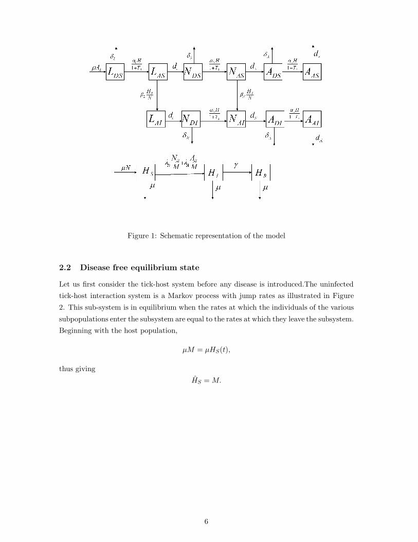
Figure 1: Schematic representation of the model

2.2 Disease free equilibrium state

Let us first consider the tick-host system before any disease is introduced.The uninfected

tick-host interaction system is a Markov process with jump rates as illustrated in Figure

2. This sub-system is in equilibrium when the rates at which the individuals of the various

subpopulations enter the subsystem are equal to the rates at which they leave the subsystem.

Beginning with the host population,

µM = µHS(t),

thus giving

HS = M.

6

Figure 2: Schematic representation of the stages of the disease-free tick-host interaction

system

For the tick population, it is at equilibrium when the incoming rates are equal to the

outgoing rates for each tick stage, (see Figure 2). Thus;

ρAAS(t) =(

δL +αLHS(t)

1 + TAS(t)

)LDS(t)

αLHS(t)1 + TAS(t)

LDS(t) = dLLAS(t)

dLLAS(t) =(

δN +αNHS(t)1 + TAS(t)

)NDS(t)

αNHS(t)1 + TAS(t)

NDS(t) = dNNAS(t)

dNNAS(t) =(

δA +αAHS(t)

1 + TAS(t)

)ADS(t)

αAHS(t)1 + TAS(t)

ADS(t) = dAAAS(t).

7

Using 1 + TAS ' TAS , we obtain;

LDS =ραAM

dA(δLTAS + αLM)ADS

LAS =ραLM

dL(δLTAS + αLM)AAS

NDS =αLM

δN TAS + αNMLDS

NAS =dLαNM

dN (δN TAS + αNM)LAS (2.1)

ADS =αNM

δATAS + αAMNDS

AAS =dNαAM

dA(δATAS + αAM)NAS

where TAS = LAS + NAS + AAS . There is no explicit solution for (2.1). However from the

equations the average number of attached ticks per host TASM at equilibrium satistifies the

condition(

δLTAS

M+ αL

)(δN

TAS

M+ αN

)(δA

TAS

M+ αA

)= αLαNαA

ρ

dA. (2.2)

For Equation (2.2) to have a positive solution for TASM , it is necessary that ρ > dA, and

from now on we assume that ρ > dA.

3 Branching process

At the early stages of an epidemic in a population which is divided into several categories of

distinguishable individuals, each having a large number of susceptible individuals and few

infected individuals; the number of infectives can often be approximated by a multi-type

branching process (Ball, 1983; Ball & Donnelly, 1995). In multi-type branching processes,

individuals in the population are categorised into a finite number of types and each individ-

ual behaves independently. An individual of a given type can produce offsprings of possibly

all types and individuals of the same type have the same offspring distribution of all type

of individuals (Ch 11, Karlin & Taylor, 1975; Ch 4, Jagers, 1975)

In the present model, the disease is spread by individuals of three types: infective

attached nymphs, infective attached adult ticks and infective hosts. An infective attached

nymph produces one infective attached adult tick when it detaches from a host, develops

to become an infected detached adult and then attaches to a host. It may also produce one

infective host if attached to a susceptible host. An infective attached adult tick produces

8

one infective host if it infects the susceptible host it is attached to. Finally, an infective host

may infect susceptible larvae and nymphs attached to it, which in turn detach, moult and

may attach to other hosts becoming attached infected nymphs and attached infected adults

respectively. Assuming the uninfected tick-host interaction system is in equilibrium at the

time when the disease is introduced in the system with a few infectives of the three types

then at the early stages the number of infectives in the population can be approximated by

a three type branching process.

3.1 Threshold condition for persistence of disease

Let the infected host be of type 0, infected attached nymphs be of type 1 and infected

attached adults be of type 2. Further let {Xij ; i, j = 0, 1, 2} be the number of infectives

of type j produced by an infective of type i and let cij = E [Xij ]. We derive the offspring

distribution and its mean matrix.

An infected host infects larvae according to a Poisson process with rate βLLASN during

its infectious period which is exponentially distributed with intensity (µ + γ). The Poisson

distribution is an approximation since assume that the average number of susceptible larvae

per host is large and constant over the infectious period so that the binomial distribution

can be approximated using Poisson. An infected larvae then becomes an infected attached

nymph with probability αN M

δN TAS+αN Mas a detached infected nymph either attaches at the

rateαNH(t)1 + TA(t)

' αN HS

TA

' αNM

TA

since we assume large populations for the susceptible ticks and hosts, or it dies at the rate

δN .

Conditioning on the length I of the infectious period, the number of infective nymphs

produced by one infective host,X01, is Poisson distributed with rate βLαN M

δN TA+αN MI LAS

M .

Thus the number of infective attached nymphs, X01, produced is mixed Poisson distributed

and the expected number is;

E [X01] = E (E[X01|I ])

= E

[βL

LA

M

αNM

δN TA + αNMI

]

=

[αNβLLA

δN TA + αNM

]E[I ]

=αNβLLA

(δN TA + αNM)(µ + γ)

as LAS = LA at the initial stages of the epidemic.

In a similar manner, an infectious host produces infective attached adult ticks when it infects

9

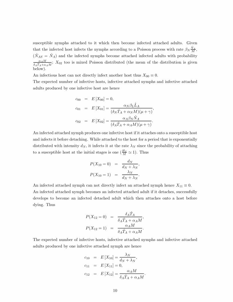
susceptible nymphs attached to it which then become infected attached adults. Given

that the infected host infects the nymphs according to a Poisson process with rate βNNAM ,

(NAS = NA) and the infected nymphs become attached infected adults with probabilityαAM

δATA+αAM; X02 too is mixed Poisson distributed (the mean of the distribution is given

below).

An infectious host can not directly infect another host thus X00 ≡ 0.

The expected number of infective hosts, infective attached nymphs and infective attached

adults produced by one infective host are hence

c00 = E [X00] = 0,

c01 = E [X01] =αNβLLA

(δN TA + αNM)(µ + γ),

c02 = E [X02] =αAβNNA

(δATA + αAM)(µ + γ).

An infected attached nymph produces one infective host if it attaches onto a susceptible host

and infects it before detaching. While attached to the host for a period that is exponentially

distributed with intensity dN , it infects it at the rate λN since the probability of attaching

to a susceptible host at the initial stages is one (HSM ' 1). Thus

P (X10 = 0) =dN

dN + λN,

P (X10 = 1) =λN

dN + λN.

An infected attached nymph can not directly infect an attached nymph hence X11 ≡ 0.

An infected attached nymph becomes an infected attached adult if it detaches, successfully

develops to become an infected detached adult which then attaches onto a host before

dying. Thus

P (X12 = 0) =δATA

δATA + αAM,

P (X12 = 1) =αAM

δATA + αAM.

The expected number of infective hosts, infective attached nymphs and infective attached

adults produced by one infective attached nymph are hence

c10 = E [X10] =λN

dN + λN,

c11 = E [X11] = 0,

c12 = E [X12] =αAM

δATA + αAM.

10

An infected attached adult tick can only produce an infected host hence X21 ≡ X22 ≡ 0.

While an infected adult is attached to a susceptible host for a time period which is expo-

nentially distributed with intensity dA, it infects the host at the rate λA before detaching.

Thus

P (X20 = 0) =dA

dA + λA,

P (X20 = 1) =λA

dA + λA.

The expected number of infective hosts, infective attached nymphs and infective attached

adults produced by one infective attached adult are hence

c20 = E [X20] =λA

dA + λA,

c21 = E [X21] = 0,

c22 = E [X22] = 0.

Let C = {cij}2i,j=0 be the expectation matrix;

C =

0 αNβLLA

(δN TA+αN M)(µ+γ)

αAβN NA

(δATA+αAM)(µ+γ)

λNdN+λN

0 αAM

δATA+αAM

λAdA+λA

0 0

.

Let the characteristic polynomial of C be f(λ);

f(λ) = λ3 − λ

(αNβLLA

(δN TA + αNM)(µ + γ)λN

dN + λN+

αAβNNA

(δATA + αAM)(µ + γ)λA

dA + λA

)

− λA

dA + λA

αNβLLA

(δN TA + αNM)(µ + γ)αAM

δATA + αAM.

The eigen-values of C are the roots of the equation,

f(λ) = 0.

From the signs of the coefficients of f(λ), we can conclude that f(λ) has an unique

positive root and since C is a non-negative matrix, the largest positive root is greater than

one if and only if f(1) < 0, that is if

R∗ =αNβLLA

(δN TA + αNM)(µ + γ)λN

dN + λN+

αAβN NA

(δATA + αAM)(µ + γ)λA

dA + λA

+αNβLLA

(δN TA + αNM)(µ + γ)αAM

δATA + αAM

λA

dA + λA> 1. (3.1)

11

R∗ is the threshold quantity for the tick-host system when the disease is introduced at

equlibrium. It increases in the attachment rates for nymphs and adults; infection rates from

nymphs and adults to hosts respectively as well as the infection rates from hosts to nymphs

and adults respectively. It decreases in the detachment rates for nymphs and adults; the

mortality rates of the nymphs and adults; the death and recovery rate of the hosts. R∗ also

depends on the average number of attached susceptible ticks per host in the system. If we

express the number of attached susceptible ticks in terms of the average number attached

per host as in Equation (2.2), we observe that R∗ also increases in the tick birth rate.

The expression R∗ can be interpreted as the average number of infectious hosts produced

indirectly by one primary infectious host: for the first term of the sum, an infectious

host produces on average αN βLLA

(δN TA+αNM)(µ+γ)infected nymphs and each nymph will infect a

susceptible host with probability λNdN+λN

; for the second term, an infectious host produces

on average αAβN NA

(δATA+αAM)(µ+γ)infected adult ticks and each adult infects a susceptible host

with probability λAdA+λA

; and finally, each of the αNβLLA

(δN TA+αN M)(µ+γ)infected nymphs produced

by an infectious host will produce an infected adult with probability αAM

δATA+αAMand the

infected adult will then infect a susceptible host with probability λAdA+λA

. Therefore R∗ is the

mean of a single type branching process approximation for the hosts. This approximation

is otherwise rather complicated to calculate as the probability distribution of the offspring

distribution is not easily attainable. A result that is almost similar to R∗ is a threshold

quantity obtained by Rosa et al. (2007) for a deterministic model for tick borne diseases

transmitted by three-host ticks. The main difference is that Rosa et al. (2007) considered

the infection transmission as related to detached (questing) ticks while in this paper we

define the infection transmission in terms of attached ticks.

3.2 Probability of a major outbreak occurring

Let the probability generating function of the offspring distribution of infectives produced

by an infective of type i (i = 0, 1, 2), be Gi(s) = E[∏2

j=0 sXij

j

], where Xij is as defined

in the previous section and s = (s0, s1, s2) . The probability that a minor outbreak of

the disease occurs given that there are ki infectives initially of each of the three types is

π = qk00 qk1

1 qk22 , where q is the solution of s = G(s) that is closest to the origin in the unit

cube [0, 1]3.

Since X01 and X02 are Poisson distributed conditioned on the infectious period I of the

host, and X00 ≡ 0; the probability generating function of the number of infected hosts,

12

infected attached nymphs and infected attached adults produced by one infected host is;

G0(s) = E[sX000 sX01

1 sX022

]= E

[E[sX01

1 sX022 |I ]

]

= E(E[sX011 |I

]E[sX022 |I

])

Let b1 = αNβLLAS

δN TA+αN M, b2 = αAβNNAS

δATA+αAM

Now,

E[sX011 |I = t

]=

∞∑

x=0

sx1

(b1t)x e−b1t

x!

= e−(b1t)(1−s1)

Similarly,

E[sX022 |I = t

]= e−(b2t)(1−s2)

Thus

E[E(sX011 |I

)(sX022 |I

)]= E[e−(b1(1−s1)+b2(1−s2))I ]

=∫ ∞

0

(µ + γ) e−(µ+γ)te−(b1(1−s1)+b2(1−s2))IdI

=µ + γ

µ + γ + b1(1− s1) + b2(1 − s2).

Substituting b1 and b2, the probability generating function is

G0(s) =(µ + γ)

(µ + γ) + αNβLLA(1−s1)

(δN TA+αN M)+ αAβNNA(1−s2)

(δATA+αAM)

(3.2)

Since X11 ≡ 0, X10 and X12 are either equal to 0 or 1, the probability generating function

of the number of infected hosts, infected attached nymphs and infected attached adults

produced by one infected attached nymph is

G1(s) = E[sX100 sX11

1 sX122

]

= E[sX100 ]E[sX12

2 ]

=(P (X10 = 0)s0

0 + P (X10 = 1)s10

) (P (X12 = 0)s0

2 + P (X12 = 1)s12

)

=[dN + λNs0

dN + λN

] [δN TA + αNMs2

δN TA + αNM

](3.3)

Finally, X21 ≡ X22 ≡ 0 and X20 is either equal to zero or one, therefore the probability

generating function of the number of infected hosts, infected attached nymphs and infected

attached adults produced by one infected attached adult is

G2(s) = E[sX200 sX21

1 sX222

]

= E[sX200 ] =

(P (X20 = 0)s0

0 + P (X20 = 1)s10

)

=dA + λAs0

dA + λA(3.4)

13

The analytic solution for s = G(s) is quite complex to derive but let s0, s1 and s2 denote

the solutions. Further let qi=min(1,si), i = 0, 1, 2,and k0, k1, k2 be the initial number

of infective hosts, attached infective nymphs and attached infective adults; then it follows

from branching process theory (Ch II, Harris, 1989) that

(i) q0 = q1 = q2 = 1 when R∗ ≤ 1 and q0 < 1,q1 < 1, q2 < 1 when R∗ > 1.

(ii) the probability of a minor outbreak occuring is π = qk00 qk1

1 qk22

(iii) the probabilty of a major outbreak is 1− π.

3.3 Endemic level

We now consider states where the system may be in equilibrium, the disease free equilib-

rium was already derived in Section 2.2. For the model defined, R∗ is used to assess this

equilibrium. If the disease is present initially in the tick-host system, then when R∗ ≤ 1

very few infections occur and the epidemic fades out quickly. On the other hand when

R∗ > 1 the epidemic may take off in the system and become endemic, taking the tick and

host populations to an infection level known as the endemic level. At this level, the tick-

host system is said to be in an endemic equilibrium state. This state is actually not a true

equilibrium when considering a finite population; eventually the disease will die out. Prior

to this the endemic equilibrium is a so called quasi-stationary distribution.

Using similar arguments as in Ethier & Kurtz (1986) and Andersson & Britton (2000),

as the tick vector and host populations increase then, by the law of large numbers, the four-

teen dimensional stochastic process converges to the trajectories of a fourteen dimensional

deterministic dynamical system.

As M → ∞, then suppose at t = 0,(

LDS(0)M

,LAS(0)

M,LAI(0)

M

)p→ (lDS(0), lAS(0), lAI(0))

(NDS(0)

M,NAS(0)

M,NDI(0)

M,NAI(0)

M

)p→ (nDS(0), nAS(0), nDI(0), nAI(0))

(ADS(0)

M,AAS(0)

M,ADI(0)

M,AAI (0)

M

)p→ (aDS(0), aAS(0), aDI(0), aAI(0)))

(HS(0)

M,HI(0)

M,HR(0)

M

)p→ (hS(0), hI(0), hR(0))

14

then at time t, 0 < t ≤ u,(u is any finite time),(

LDS(t)M

,LAS(t)

M,LAI(t)

M

)p→ (lDS(t), lAS(t), lAI(t))

(NDS(t)

M,NAS(t)

M,NDI(t)

M,NAI(t)

M

)p→ (nDS(t), nAS(t), nDI(t), nAI(t))

(ADS(t)

M,AAS(t)

M,ADI(t)

M,AAI(t)

M

)p→ (aDS(t), aAS(t), aDI(t), aAI(t))

(HS(t)

M,HI(t)M

,HR(t)

M

)p→ (hS(t), hI(t), hR(t)).

The vector

(lDS(t), lAS(t), lAI(t), nDS(t), nAS(t), nDI(t), nAS(t), aDS(t), aAS(t), aDI(t), aAI(t), hS(t), hI(t), hR(t))

is deterministic and is the solution of

l′DS(t) = ρaA(t)− δLlDS(t) − αLh(t)lDS(t)tA(t)

l′AS(t) =αLh(t)lDS(t)

tA(t)− dLlAS(t) − βLhI(t)lAS(t)

l′AI(t) = βLhI(t)lAS(t)− dLlAI(t)

n′DS(t) = dLlAS(t)− δNnDS(t) − αNh(t)nDS(t)

tA(t)

n′AS(t) =

αNh(t)nDS(t)tA(t)

− dNnAS(t) − βNhI(t)nAS(t)

n′DI(t) = dLlAI(t) − δNnDI (t)−

αNh(t)nDI(t)tA(t)

n′AI(t) =

αNh(t)nDI(t)tA(t)

+ βHNhI (t)nAS(t)− dNnAI (t) (3.5)

a′DS(t) = dNnAS(t) − δAaDS(t) − αAh(t)aDS(t)tA(t)

a′AS(t) =αAh(t)aDS(t)

tA(t)− dAaAS(t)

a′DI(t) = dNnAI(t) − δAaDI(t) −αAh(t)aDI(t)

tA(t)

a′AI(t) =αAh(t)aDI(t)

tA(t)− dAaAI (t)

h′S(t) = µ − µhS(t) − (λNnAI(t) + λAaAI(t))hS(t)

h′I(t) = (λNnAI (t) + λAaAI (t))hS(t) − µhI(t) − γhI(t)

h′R(t) = γhI(t) − µhR(t)

For the model of Equation (3.5),

15

(i) If lAI(0) = nDI(0) = nAI (0) = aDI(0) = aAI(0) = hI(0) = 0, then the tick-host

system starts in disease free equilibrium and it remains in that state.

(ii) If lAI(0) + nDI(0) + nAI (0) + aDI(0) + aAI(0) + hI (0) > 0 and R∗ ≤ 1, then the

tick-host system converges to the disease free equilibrium as t → ∞.

(iii) If lAI(0) + nDI (0) + nAI (0) + aDI(0) + aAI(0) + hI(0) > 0 and R∗ > 1, a unique

endemic equilibrium for the tick-host system exists.

Disease free equilibrium:

If lAI(0) = nDI(0) = nAI (0) = aDI(0) = aAI(0) = hI(0) = 0 the deterministic system is:

l′DS(t) = ρaA(t) − δLlDS(t) − αLh(t)lDS(t)tA(t)

l′AS(t) =αLh(t)lDS(t)

tA(t)− dLlAS(t)

n′DS(t) = dLlAS(t) − δNnDS(t) − αNh(t)nDS(t)

tA(t)

n′AS(t) =

αNh(t)nDS(t)tA(t)

− dNnAS(t)

a′DS(t) = dNnAS (t)− δAaDS(t) − αAh(t)aDS(t)tA(t)

a′AS(t) =αAh(t)aDS(t)

tA(t)− dAaAS(t)

h′S(t) = µ − µhS(t)

Equating this system of equations to zero;

lDS =ρaAtA

αL + δL tA

lAS =αLlDS

tAdL

nDS =dLtA lAS

αN + δN tA

nAS =αN nDS

tAdN

aDS =dN tAnAS

αA + δAtA

aAS =αAaDS

dAtA

hS = 1

Further lDS = lD, lAS = lA, nDS = nD, nAS = nA, aDS = aD, aAS = aA and hS = h.

16

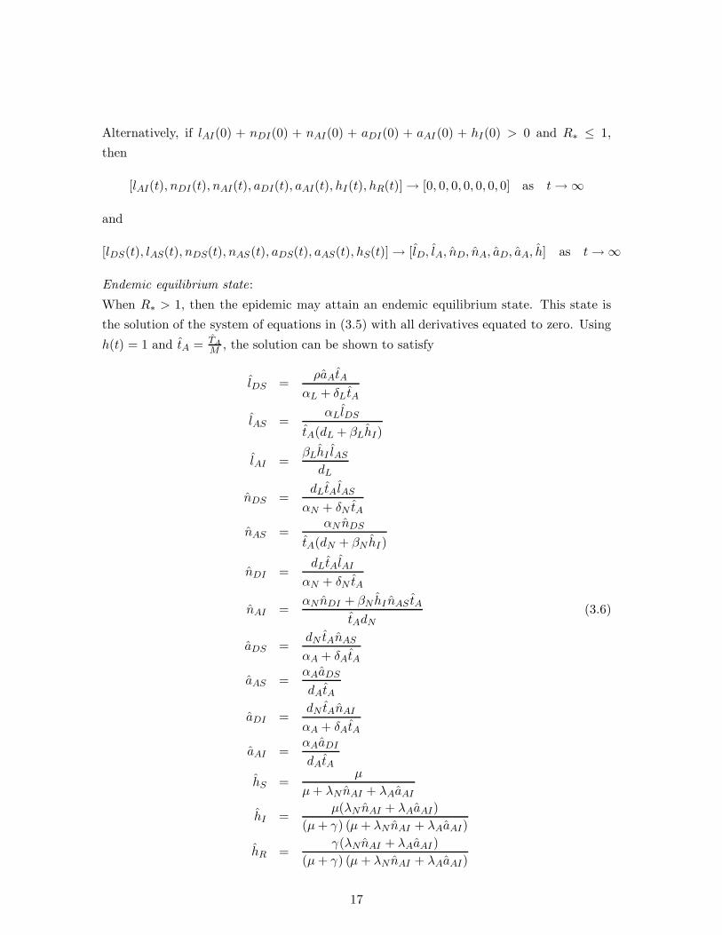
Alternatively, if lAI(0) + nDI(0) + nAI(0) + aDI(0) + aAI (0) + hI(0) > 0 and R∗ ≤ 1,

then

[lAI(t), nDI(t), nAI(t), aDI(t), aAI(t), hI(t), hR(t)] → [0, 0, 0, 0, 0, 0, 0] as t → ∞

and

[lDS(t), lAS(t), nDS(t), nAS(t), aDS(t), aAS(t), hS(t)] → [lD, lA, nD, nA, aD, aA, h] as t → ∞

Endemic equilibrium state:

When R∗ > 1, then the epidemic may attain an endemic equilibrium state. This state is

the solution of the system of equations in (3.5) with all derivatives equated to zero. Using

h(t) = 1 and tA = TAM , the solution can be shown to satisfy

lDS =ρaAtA

αL + δL tA

lAS =αLlDS

tA(dL + βLhI)

lAI =βLhI lAS

dL

nDS =dLtA lAS

αN + δN tA

nAS =αN nDS

tA(dN + βN hI )

nDI =dLtAlAI

αN + δN tA

nAI =αN nDI + βN hI nAS tA

tAdN

(3.6)

aDS =dN tAnAS

αA + δAtA

aAS =αAaDS

dAtA

aDI =dN tAnAI

αA + δAtA

aAI =αAaDI

dAtA

hS =µ

µ + λN nAI + λAaAI

hI =µ(λN nAI + λAaAI)

(µ + γ) (µ + λN nAI + λAaAI)

hR =γ(λNnAI + λAaAI )

(µ + γ) (µ + λN nAI + λAaAI)

17

In the stochastic model (MlDS , MnDS, MnDI , MaDS, MaDI , ) is the endemic level for

the detached ticks; (MlAS , MlAI , MnAS , MnAS , MaASMaAI ) for the attached ticks and

(MhS , MhI , MhR) for the host population. The tick-host system will fluctuate around this

level for a long period of time for large M before going into extinction.

4 Calibration of the models

We now compare the threshold quantity, the probability of a major outbreak occurring

and the endemic level of the present model and the one developed by Wangombe et al.

(2009) where all stages of a tick are combined in one compartment. The purpose of the

comparison is to find out if the more detailed model for the tick life cycle significantly

changes the behaviour of the model after we make the two models as similar as possible

through calibrating their model parameters.

To begin with, we define what we call the homogeneous version of the present model.

For the homogeneous setting, we let αL = αN = αA =: α, dL = dN = dA =: d, δL = δN =

δA =: δ, βL = βN =: β and λN = λA =: λ. The homogeneous version of the present model

and the model developed by Wangombe et al.(2009) will henceforth be referred to as the

homogeneous model and one-state model respectively.

4.1 Equating the population dynamics and transmission parameters

To equate the population dynamics and infection transmission parameters; let the tick

attachment rate, tick detachment rate, host birth (death) rate, host recovery rate, trans-

mission rate from host to tick and transmission rate from tick to host have the same notation

for both models.

Two parameters will differ for the two models, the tick birth rate and tick death rate.

With regard to the tick birth rates, for the one-state model, the birth rate of the ticks

is proportional to the total number of attached ticks whereas in the homogeneous model

the tick birth rate is proportional to the total number of adult attached ticks. Also with

regard to the tick death rates, for the one-state model ticks leave the system through death

of detached ticks and in the present model, the ticks leave the system through death of

detached larvae, detached nymphs, detached adults (before attaching) and attached adults

who detach and die. Thus to make the population dynamics of the tick-host system equal in

the two models we adjust the birth and death rates of the homogeneous model (see Fig.3).

18

Figure 3: An illustration of the difference between the homogeneous and one-state model,

the big boxes and arrows to and from them represent the one-state model while the smaller

boxes with arrows to and from them represent the homogeneous model.

Let ρ1 and δ1 be the tick birth and death rates for the one-state model. Then we want

ρ1(LA(t) + NA(t) + AA(t)) = ρAA(t),

δ1(LD(t) + ND(t) + AD(t)) = δ(LD(t) + ND(t) + AD(t)) + dAA(t).

To solve for ρ1 and δ1 we use Equations (2.1) and (2.2) so as to obtain the total number

of attached (detached) larvae, nymphs and adult ticks. Substituting the parameters of the

homogeneous model in Equation (2.1),

(δTA

M+ α

)3

= α3 ρ

d

TA =αM

δ

((ρ

d

) 13 − 1

).

19

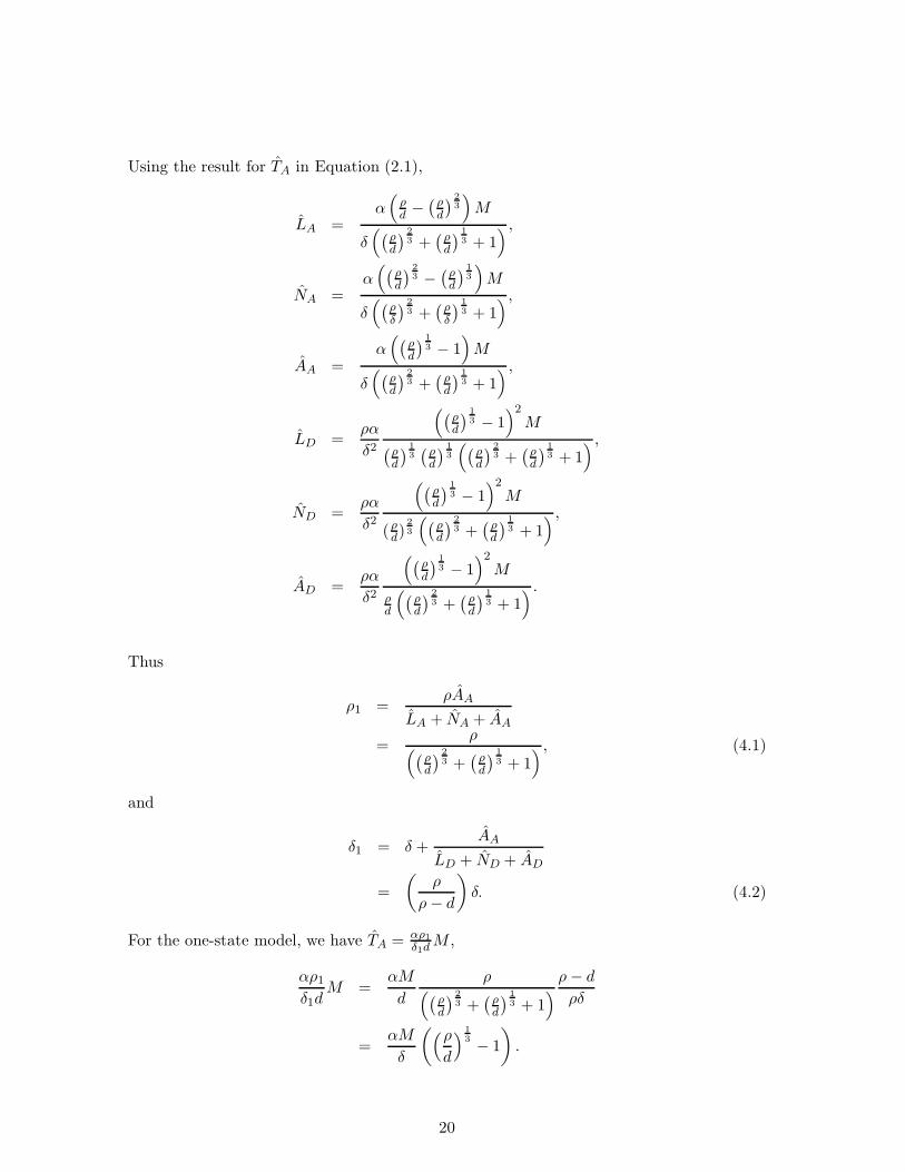
Using the result for TA in Equation (2.1),

LA =α(

ρd −

(ρd

) 23

)M

δ((ρ

d

) 23 +

(ρd

) 13 + 1

) ,

NA =α((ρ

d

) 23 −

(ρd

)13

)M

δ((ρ

δ

) 23 +

(ρδ

) 13 + 1

) ,

AA =α((

ρd

) 13 − 1

)M

δ((ρ

d

) 23 +

(ρd

) 13 + 1

) ,

LD =ρα

δ2

((ρd

) 13 − 1

)2

M

(ρd

)13(ρ

d

) 13

((ρd

) 23 +

(ρd

)13 + 1

) ,

ND =ρα

δ2

((ρd

) 13 − 1

)2

M

(ρd)

23

((ρd

) 23 +

(ρd

)13 + 1

) ,

AD =ρα

δ2

((ρd

)13 − 1

)2

M

ρd

((ρd

) 23 +

(ρd

) 13 + 1

) .

Thus

ρ1 =ρAA

LA + NA + AA

=ρ((ρ

d

) 23 +

(ρd

) 13 + 1

) , (4.1)

and

δ1 = δ +AA

LD + ND + AD

=(

ρ

ρ − d

)δ. (4.2)

For the one-state model, we have TA = αρ1δ1d M ,

αρ1

δ1dM =

αM

d

ρ((ρd

) 23 +

(ρd

) 13 + 1

) ρ − d

ρδ

=αM

δ

((ρ

d

) 13 − 1

).

20

Let the total number of detached larvae, nymphs and adults be TD, then TD = LD + ND +

AD,

TD =αM

δ2d

((ρ

d

) 13 − 1

)2

.

Similarly for the one-state model, we have

TD =αρ2

1M

dδ2= TA

ρ1

δ1

=αM

δ

((ρ

d

) 13 − 1

)ρ((ρ

d

)23 +

(ρd

) 13 + 1

) ρ− d

ρδ

=αM

δ2d

((ρ

d

) 13 − 1

)2

,

where the last equality follows from simple algebra. The tick-host system is in the same

equilibrium state for the two models.

Comparison of threshold quantity

Let the threshold quantity for the one-state model be R(1)∗ and for the homogeneous model

be R(2)∗ . From Wangombe et al. (2009), the threshold quantity for the one-state model is

βλα(1 + ρ1

d

)

δ1(λ + d)(µ + γ).

Using Equations (4.1) and (4.2)

R(1)∗ =

βαλ((ρ

d

) 13 − d

ρ

)

δ(µ + γ)(λ + d). (4.3)

Using Equation (3.1), the threshold quantity for the homogeneous model is

R(2)∗ =

βλα((ρ

d

) 23 +

(ρd

) 13 − 2

)

δ(λ + d)(µ + γ)((ρ

d

)23 +

(ρd

) 13 + 1

) . (4.4)

This implies that

R(1)∗

R(2)∗

=

((ρd

)13 − d

ρ

)((ρd

) 23 +

(ρd

) 13 + 1

)

((ρd

) 23 +

(ρd

) 13 − 2

) > 1, since ρ > d.

From this we conclude that R(2)∗ < R

(1)∗ . The new model hence always has a smaller

threshold R∗. The reason for this is that a tick can only infect at most two hosts in the

new model whereas it may infect more in the one-state model. Analysis of this result is

explored using numerical examples in Section 5. For cases where both R(1)∗ and R

(2)∗ are

larger than one, we compare the probability of major outbreak and endemic level.

21

4.2 Equating the endemic levels of attached ticks and hosts

In the previous subsection, we saw that the threshold quantity of the homogeneous model

is lower than that of the one-state model and consequently we expect the probability of a

major outbreak occurring and endemic levels of the homogeneous model to be lower. We

now adjust the calibration by making the endemic levels of the attached ticks and hosts

identical in the two models. It is not possible to have all the three endemic levels of de-

tached ticks, attached ticks and hosts identical so we exclude the detached ticks as they do

not directly lead to infection of either ticks or hosts.

Let β1 and λ1 be the infection transmission rate from host to tick and tick to host respec-

tively for the one-state model. We fix these values for the one-state model and then find

values for β and λ for the homogeneous model that give the same endemic levels. Using

numerical examples we will compare the probability of a major outbreak occurring and the

threshold quantity for the two models using this calibration.

5 Numerical examples

In this section we give examples to illustrate the results obtained in Sections 3 and 4.

5.1 The stage-structured stochastic epidemic model

The parameter values of the tick and host population dynamics as well as the infection trans-

mission are based on the work of Branagan (1973), Randolph et al. (2004), O’Callaghan

et al. (1998) and Gilioli et al. (2009). The tick attachment rates, tick detachment rates,

tick mortality rates, host birth rate, host recovery rate are reciprocal of mean time (in

days) to the event. The tick birth rate is the number of eggs laid per adult attached tick

per day while the infection transmission rates have been estimated using the same idea as

Wangombe et al. (2009), i.e for the transmission rate from nymph (adult) to host, it is

a product of the rate at which the nymph (adult) feeds on the host and the probability

that an infectious nymph (adult) transmits the infection. Similarly, the transmission rate

from host to larvae (nymph) is a product of the feeding rate and the probability that an

infectious host transmits the infection.We vary the tick attachment, tick detachment and

the infection transmission rates simultaneously for the different stages of larvae, nymph and

adult while keeping the rest of the parameters fixed. The resulting cases are sixteen and

are given in Table 1.

22

5.1.1 Threshold quantity

Using Equations (2.1), (2.2) and (3.1); we compute the threshold quantity for the sixteen

cases. The results are summarised in Table 1. From the results we observe that R∗ has the

largest value when the tick attachment rates and the infection transmission rates are high

and tick detachment rates are low. Also R∗ increases when the tick attachment rates and

infection rates are increased individually while holding all other parameters constant. The

results concur with the dependencies observed earlier in Section 3.

Table 1: Different parameter values for βL, βN , λN , λA αL , αN , αA,dL daN , dA; and thecorresponding threshold parameter R∗ with fixed values δL=0.02, δN=0.015, δA =0.005, ρ=0.75,µ=0.0006 and γ=0.05.

Case βL βN λN λA αL αN αA dL dN dA R∗

1 0.01 0.016 0.005 0.008 0.05 0.1 0.15 0.5 0.2 0.125 0.03

2 0.05 0.08 0.005 0.008 0.05 0.1 0.15 0.5 0.2 0.125 0.15

3 0.05 0.08 0.020 0.032 0.05 0.1 0.15 0.5 0.2 0.125 0.50

4 0.01 0.016 0.020 0.008 0.05 0.1 0.15 0.5 0.2 0.125 0.10

5 0.01 0.016 0.005 0.008 0.05 0.1 0.15 0.1 0.07 0.05 0.19

6 0.05 0.08 0.005 0.008 0.05 0.1 0.15 0.1 0.07 0.05 0.97

7 0.05 0.08 0.02 0.032 0.05 0.1 0.15 0.1 0.07 0.05 2.06

8 0.01 0.016 0.02 0.032 0.05 0.1 0.15 0.1 0.07 0.05 0.41

9 0.01 0.016 0.005 0.008 0.2 0.3 0.5 0.1 0.07 0.05 0.73

10 0.05 0.08 0.005 0.008 0.2 0.3 0.5 0.1 0.07 0.05 2.37

11 0.05 0.08 0.02 0.032 0.2 0.3 0.5 0.1 0.07 0.05 6.91

12 0.01 0.016 0.02 0.032 0.2 0.3 0.5 0.1 0.07 0.05 1.38

13 0.01 0.016 0.005 0.008 0.2 0.3 0.5 0.5 0.2 0.125 0.12

14 0.05 0.08 0.005 0.008 0.2 0.3 0.5 0.5 0.2 0.125 0.62

15 0.05 0.08 0.02 0.032 0.2 0.3 0.5 0.5 0.2 0.125 2.10

16 0.01 0.016 0.02 0.032 0.2 0.3 0.5 0.5 0.2 0.125 0.42

5.1.2 Probability of a major outbreak

We have solved Equations (3.2)-(3.4) to obtain the probability of a major outbreak occurring

when one infectious host, one infectious attached nymph and one infectious attached adult

are introduced into a susceptible tick-host system. For cases where R∗ > 1 out of the

16 cases above, the theoretical probabilities are summarised in Table 2. For all the other

cases where the threshold quantity is below one, the probability of a major outbreak is

23

zero. We observe that the probability of a major outbreak (1 − π) does not increase as

R∗ increases. The trend ususally is that the probability of an outbreak increases as the

threshold increases for simple epidemic models but there are exceptions for more complex

models. However for cases 10, 11 and 12 where the population dynamics parameters are

the same and only the infection transmission parameters vary, the outbreak probability

increases as R∗ increases. We ran 1000 simulations for the epidemic process for each of

the five cases where R∗ > 1 to obtain the fraction of major outbreaks occurring (1 − π)

and compared the results with the corrresponding theoretical probability (1 − π). For

cases 10, 11 and 12, the tick population (before disease introduction) was in equilibrium

with 12893 susceptible detached larvae, 781 suceptible attached larvae, 3243 susceptible

detached nymphs, 421 susceptible attached nymphs, 1463 susceptible detached adult ticks

and 448 susceptible attached adult ticks. Case 15 was in equilibrium with 8700 susceptible

detached larvae, 205 suceptible attached larvae, 3135 susceptible detached nymphs, 277

susceptible attached nymphs, 1607 susceptible detached adult ticks and 378 susceptible

attached adult ticks. Finally Case 7 was in equilibrium with 3646 susceptible detached

larvae, 202 suceptible attached larvae, 775 susceptible detached nymphs, 123 susceptible

attached nymphs, 397 susceptible detached adult ticks and 132 susceptible attached adult

ticks. The susceptible host population (before disease introduction) was 50. The disease

was introduced in the system by one infective attached nymph, one infective attached adult

tick and one infective host. Each simulation was run until either there were no infectives

in the system or there were 20 infectives in the system. It is assumed that if the number

of infectives reaches 20 the epidemic will not go extinct thus leading to a major outbreak.

The probability of a major outbreak is approximated by the fraction of simulations that

reaches 20 infectives. The results are presented in Table 2 and they are overestimates of

the theoretical probabilities though the values do not differ very much.

Table 2: Values of the theoretical probability of a major outbreak for all cases where R∗ > 1.

Case R∗ q1 q2 q3 (1− π) (1− π)

12 1.38 0.835 0.938 0.933 0.274 0.287

7 2.06 0.555 0.834 0.826 0.617 0.648

15 2.10 0.512 0.904 0.900 0.583 0.595

10 2.37 0.485 0.940 0.928 0.577 0.599

11 6.91 0.169 0.716 0.676 0.918 0.946

24

5.1.3 Endemic level

We have solved the system of equations (3.6) to obtain the endemic level for the cases where

R∗ is larger than one. The results are summarised in Tables 3-5 for the host population,

the attached ticks and detached ticks respectively. The endemic level for the infected hosts

remains fairly constant for all cases while that of the susceptible hosts varies from 7% to 34%.

For the ticks, we observe that the endemic levels vary and this is because the tick population

sizes are different depending on the population parameters as is seen in Equation (2.2). For

cases 10, 11 and 12 which have the same tick population size, the infectious proportions

increase as the threshold quantity and probability of a major outbreak increases.

One simulation was carried out for case 11 for a duration of two years, beginning the process

at the endemic level and the time averages during this period were used to obtain the

endemic proportion of the host population and the average number of attached (detached)

larvae, nymphs and adult ticks per host at the endemic level. The simulated values obtained

are hS = 0.075, hI = 0.008, hR = 0.917, lAS = 15.417, lAI = 0.06, nAS = 8.465 , nAI =

0.129, aAS = 8.681, aAI = 0.158, lDS = 255.56, nDS = 64.11, nDI = 0.3, aDS = 28.68 and

aDI = 0.47. The results are very close to the numerical solutions for case 11 given in Tables

3-5.

Table 3: Endemic proportion for host population where R∗ > 1.

Case hS hI hR

12 0.340 0.008 0.652

7 0.231 0.009 0.760

15 0.282 0.008 0.71

10 0.275 0.009 0.716

11 0.069 0.011 0.920

Table 4: Endemic proportion for attached ticks per host where R∗ > 1.

Case lAS lAI nAS nAI aAS aAI

12 15.620 0.012 8.400 0.020 8.850 0.020

7 4.040 0.018 2.430 0.030 2.620 0.030

15 4.090 0.003 5.510 0.024 7.530 0.033

10 15.560 0.061 8.310 0.120 8.740 0.120

11 15.540 0.090 8.270 0.150 8.710 0.160

To illustrate the full distribution of the simulated endemic levels of the susceptible

25

Table 5: Endemic proportion for detached ticks per host where R∗ > 1.

Case lDS nDS nDI aDS aDI

12 257.86 64.82 0.05 29.190 0.08

7 72.930 15.45 0.06 7.85 0.08

15 174.01 62.65 0.05 32.02 0.14

10 257.86 64.59 0.28 28.86 0.41

11 257.86 64.51 0.35 28.74 0.52

and infected hosts, attached nymphs and attached adult ticks for case 11, we have plotted

histograms in Figures 4-6.

2 3 4 50

0.05

0.1

0.15

0.2

0.25

0.3

0.35

0.4

0.45

0.5

Number of susceptible hosts

relat

ive fr

eque

ncy

0 1 20

0.1

0.2

0.3

0.4

0.5

0.6

0.7

Number of infected hosts

relat

ive fr

eque

ncy

Figure 4: Distribution (over time in the simulation) of susceptible and infective hosts at

the endemic level for parameters chosen for case 11.

6 7 8 9 100

0.005

0.01

0.015

0.02

0.025

0.03

Ratio of attached susceptible nymphs to hosts

relat

ive fr

eque

ncy

−0.2 0 0.2 0.4 0.60

0.02

0.04

0.06

0.08

0.1

0.12

Ratio of attached infected nymphs to hosts

relat

ive fr

eque

ncy

Figure 5: Distribution (over time in the simulation) of the number of attached susceptible

and infective nymphs per host at the endemic level for parameters chosen for case 11.

26

7 8 9 100

0.005

0.01

0.015

0.02

0.025

Ratio of susceptible adult ticks to hosts

relat

ive fr

eque

ncy

0 0.1 0.2 0.3 0.40

0.02

0.04

0.06

0.08

0.1

0.12

0.14

0.16

Ratio of infected adult ticks to hosts

relat

ive fr

eque

ncy

Figure 6: Distribution (over time in the simulation) of the number of attached susceptible

and infective adult ticks per host at the endemic level for parameters chosen for case 11.

From Figure 4, we observe that the endemic proportion of the suceptible hosts ranges

from 0.04 to 0.1 while that of the infected hosts ranges from 0 to 0.04. From Figure 5 we

observe that the average number of attached susceptible nymphs per host varies between

6.84 and 9.2 and that of the infected attached nymphs varies between 0 and 0.35. Finally

the average number of attached susceptible adult ticks varies between 7.1 and 9.1 while

that of the attached infected adult ticks varies between 0.04 and 0.27 (Figure 6). In total

there are two infectious ticks per host at the endemic level including the average number

of attached infected larvae, detached infected nymphs and detached infected adult ticks.

5.2 Comparison of the two calibrated models

5.2.1 Equal population dynamics and transmission parameters

As mentioned earlier, we fix the population dynamics and transmission parameters for the

one-state model and then obtain values for the tick birth and death parameters for the

homogeneous model so that the population dynamics are equal for both models. All other

parameters of the homogeneous model take on the same values as the one-state model.

Using Equations (4.1) and (4.2), we obtain values for ρ and d from parameter values used

in the one-state model. The threshold quantity, probability of a major outbreak occurring

and endemic levels (where applicable) are computed for five sets of parameter values. The

values are chosen so that we have a situation where both threshold quantities are larger

than 1 and also where one quantity is below 1 and the other above 1. The results for R(1)∗

and R(2)∗ are summarised in Table 6 (where R

(1)∗ refers to the one-state model and R

(2)∗ to

the homogeneous model) . Using Equations (3.2)-(3.4), we compute the probability of a

major outbreak occurring for the cases presented in Table 6 and compare the results with

those obtained for the one-state model. Both theoretical probabilities are presented in Ta-

27

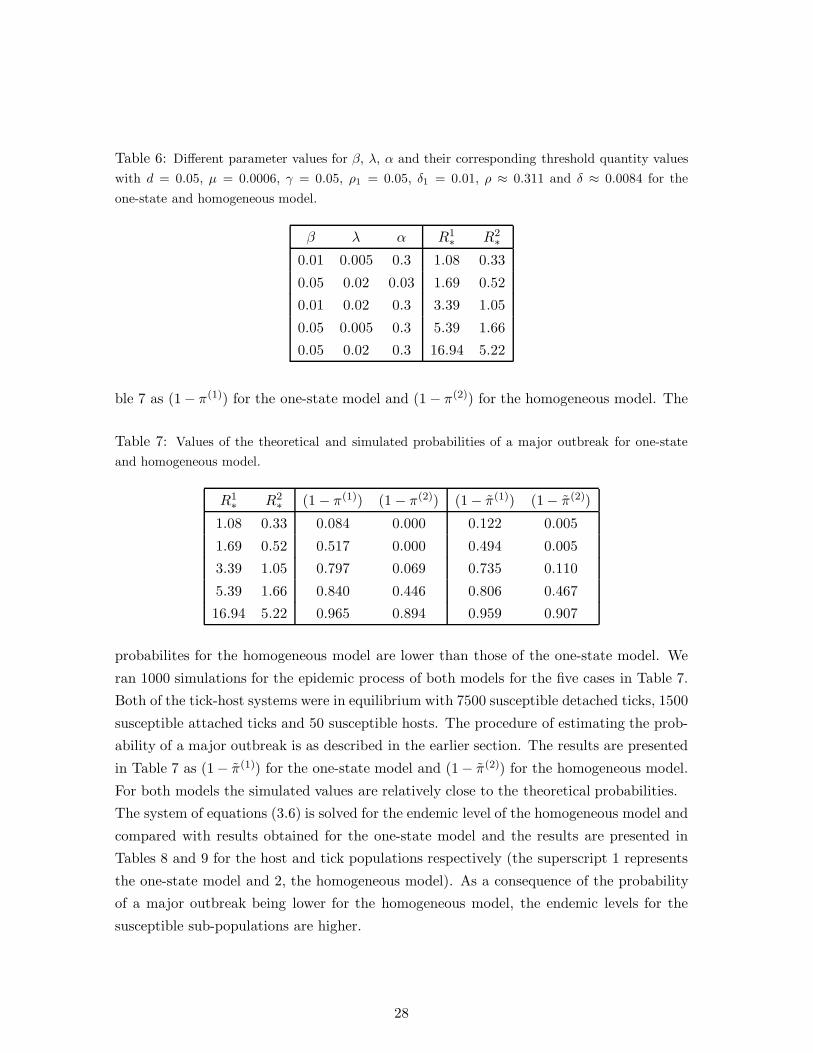
Table 6: Different parameter values for β, λ, α and their corresponding threshold quantity valueswith d = 0.05, µ = 0.0006, γ = 0.05, ρ1 = 0.05, δ1 = 0.01, ρ ≈ 0.311 and δ ≈ 0.0084 for theone-state and homogeneous model.

β λ α R1∗ R2

∗

0.01 0.005 0.3 1.08 0.33

0.05 0.02 0.03 1.69 0.52

0.01 0.02 0.3 3.39 1.05

0.05 0.005 0.3 5.39 1.66

0.05 0.02 0.3 16.94 5.22

ble 7 as (1− π(1)) for the one-state model and (1 − π(2)) for the homogeneous model. The

Table 7: Values of the theoretical and simulated probabilities of a major outbreak for one-stateand homogeneous model.

R1∗ R2

∗ (1 − π(1)) (1 − π(2)) (1− π(1)) (1− π(2))

1.08 0.33 0.084 0.000 0.122 0.005

1.69 0.52 0.517 0.000 0.494 0.005

3.39 1.05 0.797 0.069 0.735 0.110

5.39 1.66 0.840 0.446 0.806 0.467

16.94 5.22 0.965 0.894 0.959 0.907

probabilites for the homogeneous model are lower than those of the one-state model. We

ran 1000 simulations for the epidemic process of both models for the five cases in Table 7.

Both of the tick-host systems were in equilibrium with 7500 susceptible detached ticks, 1500

susceptible attached ticks and 50 susceptible hosts. The procedure of estimating the prob-

ability of a major outbreak is as described in the earlier section. The results are presented

in Table 7 as (1− π(1)) for the one-state model and (1− π(2)) for the homogeneous model.

For both models the simulated values are relatively close to the theoretical probabilities.

The system of equations (3.6) is solved for the endemic level of the homogeneous model and

compared with results obtained for the one-state model and the results are presented in

Tables 8 and 9 for the host and tick populations respectively (the superscript 1 represents

the one-state model and 2, the homogeneous model). As a consequence of the probability

of a major outbreak being lower for the homogeneous model, the endemic levels for the

susceptible sub-populations are higher.

28

Table 8: Theoretical endemic proportion for host population for one-state and homogeneous modelwhere both the threshold quantities are larger than one.

h(1)S h

(2)S h

(1)I h

(2)I h

(1)R h

(2)R

0.211 0.463 0.009 0.006 0.780 0.531

0.172 0.374 0.010 0.007 0.818 0.619

0.043 0.094 0.011 0.011 0.946 0.895

Table 9: Theoretical values of the average number of attached ticks and detached ticks per host forone-state and homogeneous model where both threshold quantities are larger than one.

t(1)AS t

(2)AS t

(1)AI t

(2)AI t

(1)DS t

(2)DS t

(1)DI t

(2)DI

29.89 29.94 0.11 0.06 149.72 149.88 0.28 0.12

29.42 29.68 0.58 0.32 148.60 149.5 1.40 0.5

29.33 29.54 0.67 0.46 148.30 149.27 1.70 0.73

5.2.2 Equal endemic levels for attached ticks and hosts

We now calibrate the two models by instead equating the endemic levels as described in

Section 4.2. We fix values for β1, the infection transmission rate from host to tick and λ1,

the infection transmission rate from tick to host for the one-state model and then choose

values for β and λ for the homogeneous model so that the endemic levels coincide. Using

the results obtained and the values of the other parameters as given in the earlier example,

we compute the probability of a major outbreak occurring and the threshold quantity. The

results are summarised in Table 10.

Table 10: Infection parameters, threshold quantity, theoretical and simulated probability of a majoroutbreak for one-state and homogeneous models with equal endemic levels for attached ticks andhosts.

β1 β λ1 λ R(1)∗ R

(2)∗ (1− π(1)) (1− π(2)) (1 − π(1)) (1 − π(2))

0.01 0.014 0.005 0.008 1.08 0.69 0.084 0.000 0.122 0.01

0.05 0.069 0.02 0.032 1.69 0.99 0.517 0.000 0.494 0.008

0.01 0.014 0.02 0.032 3.39 2.00 0.797 0.676 0.735 0.696

0.05 0.069 0.005 0.008 5.39 3.48 0.840 0.771 0.806 0.780

0.05 0.069 0.02 0.032 16.94 9.85 0.965 0.961 0.959 0.964

The threshold quantity is still considerably lower for the homogenous model. As for the

probability of a major outbreak occurring, we observe that the values are relatively close

29

for the last case in Table 10 but differ considerably for the other two cases. We conclude

that even though we increase the disease transmission rates, the threshold quantity and

probability of a major outbreak are still lower for the homogeneous model. As in the

previous subsection, we ran 1000 simulations using the same procedure for the homogeneous

model with the new parameters for β and λ and the results of the proportions that do not

go extinct are presented in Table 10 as (1 − π(2)). Again the proportions are close to the

theoretical probabilities. For the first two cases in Table 10 where R(2)∗ < 1, the endemic

levels are very low and not sustainable for practical purposes. We expect that the endemic

state is unstable and hence the disease free state is stable.

6 Discussion

In the present paper we have formulated a stochastic model for the spread of tick-borne

diseases which incorporates the life stage structure of the ticks. The aim of this was to

develop a more realistic model than the one developed earlier by Wangombe et al. (2009).

The threshold condition for the persistence of the disease, the probability of a major out-

break and endemic level of the disease are derived. The threshold condition is defined in

terms of a threshold quantity which depends on the population dynamics parameters of the

tick-host system as well as the transmission parameters, Equation (3.1). In Sections 3.1

and 5.1.1, it was shown that the number of infectives in the tick-host system increase when

the tick attachment rates of the different stages of the tick, the transmission rates from

host to larvae (nymph) and the transmission rate from nymph (adult) to host increase;

and decrease when the tick detachment rates for the different stages of the tick increase.

Thus these parameters play a key role in the transmission dynamics of the disease when

the tick-host system is in equilibrium. Any control strategy for the disease should therefore

aim for a reduction in the parameters that enhance the disease and/or an increase in those

that lead to a reduced spread. Similar results for the threshold quantity can be obtained

using deterministic models as shown by Rosa et al. (2007). However the stochastic version

has the advantage that we can calculate the probability of a major outbreak occurring,

something which is not possible for a deterministic model.

We also compared the present three stage model with the one stage model in Wangombe

et al. (2009). This is done to determine if anything is gained by making the model more

complicated. To make meaningful comparisons, we defined a homogeneous version of the

present model, and then calibrated the parameters of the homogeneous version and the one

stage model of Wangombe et al. (2009). From the results in Sections 4 and 5.2, we see that

the homogeneous version has smaller threshold and lower probability of a major outbreak

despite the calibrations made of the two models. We therefore conclude that the two models

30

are genuinely different and that the present model gives a more realistic representation of

the transmission dynamics of the disease. The main reason for better realism, as mentioned

earlier, is that a tick in the present model infects fewer hosts (at most two in its life cycle)

than in the previous model. By neglecting that a tick goes through several stages, the one

stage model can be above threshold whereas in fact it is below when admitting the tick life

stages. From a prevention perspective this is infact good news: The necessary amount of

change in various parameters so as to come below threshold is smaller if admitting the tick

life stages.

The present model has some limitations that could be incorporated to make the model

more realistic. For example we assume that there is no increased mortality of infectious hosts

due to the disease and yet as mentioned in the Introduction, the tick-borne diseases do lead

to death of cattle. One possible extension of the present model is hence to consider increased

mortality due to the disease as done in O’Callaghan et al. (1998). The role of wildlife

that share open fields with the cattle is not considered and their presence could influence

the population dynamics of the ticks and therefore lead to a dilution or enhancement of

the disease. The role of carrier cattle may also be considered as they may lead to an

enhancement of the disease even though their ability to transmit the infection is greatly

reduced (O’Callaghan et al. (1998)). Lastly, assumptions like exponential life length for

hosts and that attachment rates depend on the total number of attached ticks (rather than

the number of attached ticks on the specific host in question) can be relaxed to make the

model more realistic.

Acknowledgement

Anne Wangombe is grateful to the International Science Programme(ISP) at Uppsala Uni-

versity, Sweden, for financial support.

31

References

ANDERSSON, H & BRITTON, T. (2000) Stochastic epidemic models and their statistical

analysis. Springer Lecture Notes in Statistics vol.151. New York:Springer-Verlag

BALL, F.(1983): The threshold behaviour of epidemic models. J Appl. Prob, 20, 227-242.

BALL, F. & DONNELLY, P. (1995) Strong approximations for epidemic models. Stoch.

Proc. Appl., 55, 1-21.

BRANAGAN, D. (1973) Observations on the developmental and survival of Ioxdid tick

Rhipicephalus appendiculatus Neumann, 1901 under quasi-natural conditions in Kenya.

Trop. Anim. Prod, 5, 153-165.

ETHIER, S. & KURTZ, T.G. (1986) Markov processes: Characterisation and Convergence.

New York: Wiley & Sons

GILBERT, L., NORMAN, R., LAURENSON, M., REID, H. & HUDSON,P. (2001) Disease

persistence and apparent competition in a three host community: an empirical analytical

study of large scale wild populations. J. Anim. Ecol., 70, 1053-1061.

GILIOLI, G., GROPPI, M., VESPERONI, M.P., BAUGARTNER, J. & GUTIERREZ, A.P

(2009) An epidemiological model of East Coast Fever in African livestock. Ecol. Model.,

220, 1652-1662.

HARRIS E.T (1989) The theory of branching processes. Dove Publications, New York.

JAGERS, P. (1975) Branching processes with biological applications. New York: Wiley.

KARLIN, S. & TAYLOR, H. (1975) A first course in stochastic processes, 2nd ed. New

York: Academic Press.

MEDLEY, G.F. (1994) The transmission dynamics of Theileria parva: Proceedings of a

workshop on modelling vector vector borne and other parasitic diseases, 13-24.

MINJAUW, B. & McLEOD, A. (2003) Tick-borne diseases and poverty. The impact of

ticks and tick-borne diseases on the livelihood of small-scale and marginal livestock owners

in India and Eastern and Southern Africa. Research report, DFID Animal Health Pro-

gramme, Center for Tropical Veterinary Medicine, University of Edinburgh, UK.

MWAMBI, H. (2002) Ticks and tick borne diseases in Africa: a disease transmission model.

IMA J. Math. Appl. Med. Biol., 19, 275-292.

MWAMBI, H.G, BAUMGARTNER,J. & HADELER,J. (2000) Ticks and tick-borne dis-

eases: a vector-host interaction model for the brown ear tick (Rhipicephalus appendicula-

tus). Stat. Methods Med. Res., 9, 279-301.

NORMAN, R., ROSA, R., HUDSON, P.J, & PUGLIESE, A. (2003) Threshold for dis-

ease persistence in models for tick-borne infections including non-viraemic transmission,

extended feeding and tick aggregration. J.Theor. Biol., 224, 359-376.

32

O’CALLAGHAN, C., MEDLEY, G., PERRY, B.D. & PETER, T. (1998) Investigating

the epidemiology of heartwater(Cowdria ruminantium) infection by means of a transmis-

sion dynamics model. Parasitology, 117, 49-61.

PERRY, B.D., MEDLEY, G.F. & YOUNG, A.S. (1993) Preliminary analysis of transmis-

sion dynamics of Theileria parva in East Africa. Parasitology, 106, 251-264.

RANDOLPH, S.E (2004) Tick ecology: processes and patterns behind the epidemiological

risk posed by ixodid ticks as vectors. Parasitology, 129, S37-S65.

ROSA,R., PUGLIESE,A. (2007) Effects of tick population dynamics and host densities on

the persistence of tick-borne infections. Math. Biosci., 208, 216-240.

TORR, S., EISLER, M., COLEMAN, P., MORTON, J. & MACHILA, N. (2002) Integrated

control of ticks and tsetse. Natural Resources International report.

WANGOMBE, A., ANDERSSON, M. & BRITTON, T. (2009) A stochastic epidemic model

for tick borne diseases: initial stages of an outbreak and endemic levels (submitted).

33

Department of MathematicsStockholm University

Mathematical statisticsDecember 2009

www.math.su.se

Mathematical statisticsDepartment of MathematicsStockholm UniversitySE-106 91 Stockholm