Step-by-Step 1 – Protect a Web viewStep-by-Step 3 – Allow Multiple Users to Edit a...

MSITA: Excel 2013 Chapter 11

Lesson 11: Securing & Sharing WorkbooksStep-by-Step 1 – Protect a WorksheetGET READY. LAUNCH Excel.1. OPEN 11 Contoso Employees from the data files for this lesson.2. On the SSN worksheet, select cell G4.3. Click the FORMULAS tab, choose Math & Trig and select RANDBETWEEN. This formula creates a random number for each employee that can be used for identification purposes.4. In the Function Arguments dialog box, in the Bottom box, type 10000 and in the Top box, type 99999, as shown in Figure 11-2. Click OK. As one of the first steps in information security, employees are usually assigned an Employee ID number that can replace Social Security numbers for US employees, Social Insurance numbers for Canadian employees, and National Insurance numbers for UK employees on all documents.5. Double-click the fill handle in cell G4 to copy the range to G5:G33. Each employee is now assigned a random five-digit ID number.6. With the range G4:G33 already selected, on the HOME tab, click Copy. Click the Paste arrow, and then click Paste Values.7. With G4:G33 selected, on the HOME tab, click Format and then select Format Cells. Click the Protection tab and verify that Locked is checked. This prevents employee ID numbers from being changed when the worksheet has been protected. Click OK.8. On the HOME tab, click the Sort & Filter button and select Sort Smallest to Largest. On the Sort Warning dialog box, select Continue with the current selection, and then click Sort.9. Select cells C4:D33. On the HOME tab, click Format. Notice that the Lock Cell command appears selected, meaning the cells are locked by default. Click Lock Cell to turn off the protection on these cells to allow these cells to change.10. Click on the REVIEW tab, and in the Changes group, click Protect Sheet.11. In the Password to unprotect sheet box, type L11!e01. The password is not displayed in the Password to unprotect sheet box. Instead, asterisks (*) are displayed as shown in Figure 11-3. Click OK.12. You are asked to confirm the password. Type L11!e01 again and click OK. You have just created and confirmed the password that will lock the worksheet. Passwords are meant to be secure. This means that all passwords are case sensitive. Thus, you must type exactly what has been assigned as the password—uppercase and lowercase letters, numbers, and symbols.13. SAVE the workbook as 11 Payroll Data Solution. CLOSE the workbook.PAUSE. LEAVE Excel open for the next exercise.

of 18


Step-by-Step 2 – Protect a WorkbookGET READY. OPEN the 11 Payroll Data Solution workbook that you saved and closed in the previous exercise.1. Click cell G11 and try to type a new value in the cell. A dialog box informs you that you are unable to modify the cell because the worksheet is protected. Click OK to continue.2. Click cell D4 and change the number to 1. You can make changes to cells in columns C and D because you unlocked the cells before you protected the worksheet. Click Undo to reverse the change.3. Click the Performance worksheet tab and select cell D4.4. On the HOME tab, in the Cells group, click the Delete arrow, and click Delete Sheet Rows. Dr. Bourne’s data is removed from the worksheet because this worksheet was left unprotected.5. Click Undo to return Dr. Bourne’s data.6. Click the SSN worksheet tab. Click the RE VIEW tab, and in the Changes group, click Unprotect Sheet.7. Type L11!e01 (the password you created in the previous exercise) and click OK.8. Click cell D11. Type 8, press Tab three times, and then type 17000 (see Figure). Press Tab.9. On the REVIEW tab, in the Changes group, click Protect Sheet. In the two dialog boxes, type the original password for the sheet L11!e01 to again protect the SSN worksheet.10. On the REVIEW tab, in the Changes group, click Protect Workbook. The Protect Structure and Windows dialog box shown in Figure 11-5 opens. Select the Protect workbook for Structure check box in the dialog box , if it isn’t already selected.11. In the Password box, type L11&E02, and then click OK. Confirm the password by typing it again and click OK.

The workbook password is optional, but if you do not supply a password, any user can unprotect the workbook and change the protected elements.

12. To verify that you cannot change worksheet options, right-click the Performance worksheet tab and notice the dimmed commands shown in Figure 11-6.13. Press Esc and click the FILE tab. Select Save As, and then click the Browse button.14. In the Save As dialog box, click the Tools button. The shortcut menu opens (see Figure 11-7).15. Select General Options. The General Options dialog box opens. In the General Options dialog box, in the Password to open box, type L11&E02. Asterisks appear in the text box as you type. Click OK.16. In the Confirm Password dialog box, reenter the password, and then click OK. You must type the password exactly the same each time.17. Click Save and click Yes to replace the document. As the document is now saved, anyone who has the password can open the workbook and modify data contained in the Performance

of 18


worksheet because that worksheet is not protected. However, to modify the SSN worksheet, the user must also know the password you used to protect that worksheet in the first exercise.

When you confirm the password to prevent unauthorized viewing of a document, you are reminded that passwords are case-sensitive. If the password you enter in the Confirm Password dialog box is not identical to the one you entered in the previous dialog box, you will receive an error message. Click OK to close the error message and reenter the password in the Confirm Password dialog box.

18. CLOSE the workbook and OPEN it again.19. In the Password box, type 111 and click OK. This is an incorrect password to test the security. You receive a dialog box warning that the password is not correct. Click OK.PAUSE. LEAVE Excel open for the next exercise.

Step-by-Step 3 – Allow Multiple Users to Edit a Workbook SimultaneouslyGET READY. LAUNCH Excel if it is not already running.1. CREATE a new blank workbook.2. In cell A1, type Sample Drugs Dispensed and press Tab.3. Select cells A1:D1. On the HOME tab, in the Alignment group, click Merge & Center.4. Select cell A1, click Cell Styles, and in the Cell Styles gallery that appears, click Heading 1.5. Beginning in cell A3, enter the following data:

MEDICAL ASSISTANT DRUG PATIENT DATEDellamore, Luca Cipro Chor, AnthonyHamilton, David Ketek Brundage, MichaelHoeing, Helge Lipitor Charles, MatthewMurray, Billie Jo A ltace Bishop, ScottDellamore, Luca Zetia Anderson, NancyHamilton, David Cipro Coleman, PatHoeing, Helge Avelox Nayberg, AlexMurray, Billie Jo Norvasc Kleinerman, Christian

6. In the Date column, apply today’s date to the previous records.7. Select cells A3:D3 and apply the Heading 3 style.8. Increase the column widths to see all the data.9. SAVE the workbook as 11 Sample Medications Solution.10. Click the RE VIEW tab, and then, in the Changes group, click Share Workbook.11. In the Share Workbook dialog box, click Allow changes by more than one user at the same time. Your identification will appear in the Who has this workbook open now box, as shown in Figure w. Click OK.12. Click OK when prompted and the action will save the workbook.

of 18


13. In the Changes group, click Protect Shared Workbook. Select the Sharing with track changes check box in the Protect Shared Workbook dialog box. Click OK.14. Notice that [Shared] appears in the title bar.15. SAVE and CLOSE the workbook.PAUSE. LEAVE Excel open for the next exercise.

Step-by-Step 4 – Use the Document InspectorGET READY. OPEN 11 Contoso Employee IDS from the files for this lesson.1. Click the FILE tab, click Save As, click Browse, and navigate to the Lesson 11 folder. In the File name box, type 11 Employee ID Doc Inspect Solution to save a copy of the workbook. Click the Save button.

It is a good idea to perform an inspection on a copy of your workbook because you might not be able to restore hidden content that you remove in the inspection process. If you attempt to inspect a document that has unsaved changes, you will be prompted to save the document before completing the inspection.

2. Click the FILE tab. Then, with Info selected, click the Check for Issues button in the middle pane of the Backstage view. Next, click Inspect Document. The Document Inspector dialog box opens, as shown in Figure 11-9.3. Click Inspect. The Document Inspector changes to include some Remove All buttons.4. Click Remove All for Comments and Annotations.

You must remove each type of hidden data individually. You can inspect the document again after you remove items.

5. Click Remove All three times for Document Properties and Personal Information, Hidden Rows and Columns, and Hidden Worksheets. Headers and Footers should be the only hidden item remaining (see Figure 11-10).6. Click the Close button to close the Document Inspector dialog box.7. SAVE the workbook.PAUSE. CLOSE the workbook.

Step-by-Step 5 – Mark a Document as FinalGET READY. OPEN 11 Contoso Employee IDS.1. SAVE the workbook in the Lesson 11 folder as 11 Employee ID Final Solution.2. Click the FILE tab and in Backstage view, click the Protect Workbook button. Click Mark as Final, as shown in Figure 11-11 in the MOAC text.3. An Excel message box opens, indicating that the workbook will be marked as final and saved. Click OK.

of 18


4. Another Excel message box explains that the document has been marked as final. This also means that the file has become read-only, meaning you can’t edit it unless you click the Edit Anyway button. Click OK. Notice a Marked as Final icon appears in the status bar (See Figure 11-12).PAUSE. LEAVE the workbook open for the next exercise.

Step-by-Step 6 – Distribute a Workbook by Email From ExcelGET READY. USE the workbook from the previous exercise.

Note that you must have an email program and Internet connection to complete the following exercises.

1. Click the FILE tab and click Share. In the Share window, click Email. Click the Send as Attachment button. When you have Office 2013 installed, this feature will open Outlook by default. If you have changed your environment, your own personal email program will open. Notice that Excel automatically attaches the workbook to your email message.2. In the To field, type [your instructor’s email address].3. In the subject line, replace the current entry with Employee Final Attached as per request.4. In the email message body, type The Employee ID Final workbook is attached.5. Click Send. Your email with the workbook attached to it will now be sent to your instructor.CLOSE the workbook. LEAVE Excel open for the next exercise.

Step-by-Step 7 – Distribute a Worksheet as an Email MessageGET READY. OPEN the 11 Contoso Employee IDS file.1. SAVE the file in the Lesson 11 folder as 11 Employee ID Recipient Solution.2. Click the FILE tab and click Options. The Excel Options dialog box opens.3. Click Quick Access Toolbar. In the Choose commands from field, click Email. In the center bar between the left and right fields, click Add. This step adds the Email button to the Quick Access Toolbar.4. In the Choose commands from drop-down box, click All Commands. Click in the list and type the letter s, and then scroll and find Send to Mail Recipient and click to highlight it. In the center bar between the left and right fields, click Add. This step adds this command to the Quick Access Toolbar.5. Click OK to save both commands to the Quick Access Toolbar.6. On the Quick Access Toolbar, click Send to Mail Recipient. The E-mail dialog box opens as shown in Figure 11-13.7. Click the Send the current sheet as the message body option, and then click OK. The email window is now embedded in your Excel screen with the current worksheet visible as the body of the email.8. In the To field, type [your instructor’s email address] and keep the name of the file in the Subject line. This is automatically added for you.

of 18


9. In the Introduction, type Please Review (see Figure 11-14).10. Click the Send this Sheet button, as illustrated in Figure 11-14. Click OK.11. There might be a message about hidden rows or columns. If prompted to continue, click OK.12. SAVE the workbook.CLOSE the workbook. LEAVE Excel open for the next exercise.

Step-by-Step 8 – Distribute a Workbook from within your Email ProgramGET READY. LAUNCH your email program.1. Create a new email message.2. In the To field, type [your instructor’s email address].3. In the Subject line, type Employee ID Final ready to send.4. Click Attach File.5. Navigate to the Lesson 11 folder where you saved Employee ID Final. Click the filename, and then click Insert.6. Click Send.CLOSE the email program. LEAVE Excel open for the next exercise.

Step-by-Step 9 – Share a Workbook in the CloudGET READY. OPEN 11 Contoso Patient Visits.1. SAVE the workbook to the Lesson 11 folder as 11 Patient Visits SkyDrive Solution.2. You will save this again to the SkyDrive. Click FILE and then click Share. There are two options to choose from before the file is saved to the SkyDrive. Invite People is selected by default, as shown in Figure 11-15.3. Click the Save To Cloud button. The Save As pane opens.4. Click the SkyDrive option and click the Browse button.5. In the Save As dialog box, scroll down to the Public folder and click Save to save the file on your Public SkyDrive folder.6. In the Type names or e-mail addresses box, type [the email address of your instructor].7. In the next box, type Please review my assignment.8. You can choose whether the instructor can view or edit the Excel file. Click on the arrow after Can edit and change this to Can view.9. Click the Share button.10. Open a new email message in your email program and address the email to yourself with a CC to your instructor. Type Patient Visits for the Subject. In the Body of the message, type View, press Enter, and type Edit.11. Return to Excel and click the Get a Sharing Link button.12. Under View Link, click the Create Link button, and then after the word View, COPY and PASTE the link shown to your email message, and then press Enter after the link in the email. The link should change to a hyperlink depending on your email program.

of 18


13. Return to Excel. Under Edit Link, click the Create Link button. Both links show on the screen (see Figure 11-17).14. COPY and PASTE the Edit Link after the word Edit in your email message and press Enter after the link. SEND the email message.15. When the message comes to your Inbox, click the Edit Link to take you to the Internet and the Excel Web app. If necessary, click the EDIT WOR KBOO K menu item and choose Edit in Excel Web App. Explore the Web interface as shown in Figure 11-18.16. CLOSE the Web browser without saving the document, close your email program, and click the Return to Document button in Excel.SAVE and CLOSE the workbook. LEAVE Excel open for the next exercise.

Step-by-Step 10 – Turn Track Changes On and OffGET READY. OPEN the 11 Contoso Assignments workbook for this lesson.1. SAVE the workbook as 11 Assignments Solution in the Lesson 11 folder.2. On the REVIEW tab, in the Changes group, click the Protect and Share Workbook button. The Protect Shared Workbook dialog box opens.3. In the dialog box, click Sharing with track changes. When you choose this option, the Password text box becomes active. You can assign a password at this time, but it is not necessary. Click OK.4. Click OK when asked if you want to continue and save the workbook. You have now marked the workbook to save tracked changes.PAUSE. LEAVE the workbook open for the next exercise.

Step-by-Step 11 – Set Track Change OptionsGET READY. USE the workbook from the previous exercise.1. On the REVIEW tab, in the Changes group, click Share Workbook. The Share Workbook dialog box opens.2. Click the Advanced tab (see Figure 11-19).

of 18


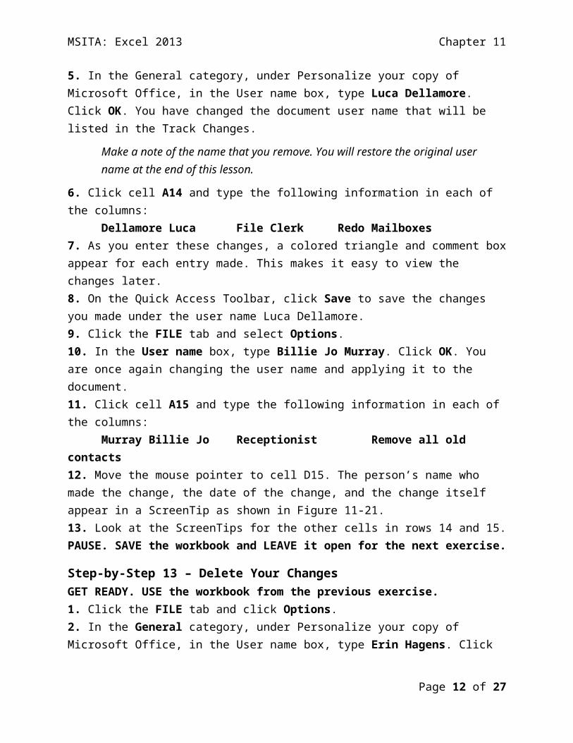
3. In the Keep change history for box, click the scroll arrow to display 35.4. Click the automatically every option button so the fi le automatically saves every 15 minutes (the default).5. Click OK to accept the default settings for the remainder of the options.PAUSE. SAVE the workbook and LEAVE it open for the next exercise.

Step-by-Step 12 – Insert Tracked ChangesGET READY. USE the workbook from the previous exercise.1. On the Review tab, in the Changes group, click track Changes. In the drop-down list that appears, click Highlight Changes. The Highlight Changes dialog box appears.2. The Track changes while editing box is inactive because Track Changes was activated when you shared the workbook. In the When drop-down box, click the down arrow, and then click all. In the Who check box and drop-down list, check the box and select everyone. The dialog box should appear as shown in Figure 11-20 in the MOAC text.3. The Highlight changes on screen option is already selected. Click OK. If a warning box appears, click OK to accept.4. Click the FILE tab and click Options. The Excel Options dialog box opens.5. In the General category, under Personalize your copy of Microsoft Office, in the User name box, type Luca Dellamore. Click OK. You have changed the document user name that will be listed in the Track Changes.

Make a note of the name that you remove. You will restore the original user name at the end of this lesson.

6. Click cell A14 and type the following information in each of the columns: Dellamore Luca File Clerk Redo Mailboxes

of 18


7. As you enter these changes, a colored triangle and comment box appear for each entry made. This makes it easy to view the changes later.8. On the Quick Access Toolbar, click Save to save the changes you made under the user name Luca Dellamore.9. Click the FILE tab and select Options.10. In the User name box, type Billie Jo Murray. Click OK. You are once again changing the user name and applying it to the document.11. Click cell A15 and type the following information in each of the columns:

Murray Billie Jo Receptionist Remove all old contacts12. Move the mouse pointer to cell D15. The person’s name who made the change, the date of the change, and the change itself appear in a ScreenTip as shown in Figure 11-21.13. Look at the ScreenTips for the other cells in rows 14 and 15.PAUSE. SAVE the workbook and LEAVE it open for the next exercise.

Step-by-Step 13 – Delete Your ChangesGET READY. USE the workbook from the previous exercise.1. Click the FILE tab and click Options.2. In the General category, under Personalize your copy of Microsoft Office, in the User name box, type Erin Hagens. Click OK. You have again changed the user of the workbook for change tracking purposes.3. Select cell A16 and type the following information in each of the columns:

Hagens Erin Receptionist Clean all corridors4. Click cell D13, and then edit the cell so corridors is spelled correctly. Change corredors to corridors.

Undo is inactive in a shared workbook. If you accidentally replace your data or another user’s data, you need to reject the change to restore the data you replaced.

5. On the REVIEW tab, click Track Changes, and then from the drop-down menu that displays, click Accept/Reject Changes. Excel displays a message box confirming that you want to save the workbook. Click OK. The Select Changes to Accept or Reject dialog box opens.6. In the Select Changes to Accept or Reject dialog box, click the Who drop-down arrow and select Erin Hagens, and then click OK. You have just asked Excel to return only the tracked changes made by Erin Hagens (see Figure 11-22). Excel highlights row 16 with green dashes where Hagens’ information is typed in.

The order of the accept or reject changes may appear differently. Accept the change in D13 but reject all other changes.

7. Click Reject. All four entries are removed.8. When cell D13 is selected for the correction of the spelling of corridors, click Accept.

of 18


PAUSE. SAVE the workbook and LEAVE it open for the next exercise.

Step-by-Step 14 – Accept Changes from Another UserGET READY. USE the workbook from the previous exercise.1. Click the FILE tab and click Options.2. In the General category, under Personalize your copy of Microsoft Office, in the User name box, type Jim Giest. Click OK.3. Click Track Changes and select Accept/Reject Changes from the drop-down list.4. Not yet reviewed will be selected by default. In the Who box, select Luca Dellamore. Click OK. The Accept or Reject Changes dialog box is displayed.5. Click Accept to accept each of the changes Luca made. The Accept or Reject Changes dialog box closes when you have accepted all changes made by Luca Dellamore.PAUSE. SAVE the workbook and LEAVE it open for the next exercise.

Step-by-Step 15 – Reject Changes from Another UserGET READY. USE the workbook from the previous exercise.1. Click Track Changes and click Accept/Reject Changes.2. On the right side of the Where box, click the Collapse Dialog button.3. Select the data in row 15 and click the Expand Dialog button. Click OK to close the Select Changes to Accept or Reject dialog box. The Accept or Reject Changes dialog box is displayed.4. Click Reject All. A dialog box will open to ask you if you want to remove all changes and not review them. Click OK. The data is removed and row 15 is now blank.5. SAVE the workbook in the Lesson 11 folder as 11 Assignments Edited Solution.PAUSE. LEAVE the workbook open for the next exercise.

Step-by-Step 16 – Remove Shared Status from a WorkbookGET READY. USE the workbook from the previous exercise.1. On the RE VIEW tab, in the Changes group, click Track Changes, and then click Highlight Changes.2. In the When box, All is selected by default. This tells Excel to search through all tracked changes made to the worksheet.3. Clear the Who and Where check boxes if they are selected.4. Click the List changes on a new sheet check box. Click OK. A History sheet is added to the workbook.5. On the History worksheet, in the corner of the worksheet adjacent to the first column and first row, click the Select All button. Click the HOME tab, and then in the Clipboard group, click the Copy button.6. Press Ctrl + N to open a new workbook.7. In the new workbook, on the HOME tab, in the Clipboard group, click Paste.

of 18


8. SAVE the new workbook as 11 Assignments History Solution. CLOSE the workbook. It is a good idea to print the current version of a shared workbook and the change history, because cell locations in the copied history may no longer be valid if additional changes are made.9. In the shared workbook, click on the RE VIEW tab, click Unprotect Shared Workbook and then click Share Workbook. The Share Workbook dialog box is displayed. On the Editing tab, make sure that Jim Giest (the last user name changed in File Options) is the only user listed in the Who has this workbook open now list.10. Clear the Allow changes by more than one user at the same time. Click OK to close the dialog box.11. A dialog box opens to prompt you about removing the workbook from shared use. Click Yes to turn off the workbook’s shared status. The word Shared is removed from the title bar.12. SAVE and CLOSE the workbook.PAUSE. LEAVE Excel open for the next exercise.

Step-by-Step 17 – Insert a CommentGET READY. OPEN the 11 Contoso Personnel Evaluations file for this lesson.1. Select cell E11. On the RE VIEW tab, in the Comments group, click New Comment. The comment text box opens for editing.2. Type Frequently late to work as shown in Figure 11-23 in the MOAC text.3. Click cell D8. Press Shift + F2 and type Currently completing Masters degree program for additional certification. Click outside the comment box. The box disappears and a red triangle remains in the upper-right corner of the cell the comment was placed in.4. Click cell E4. Click New Comment and type Adjusted hours for family emergency.5. Click cell F10. Click New Comment and type Consider salary increase.6. SAVE the file as 11 Evaluations Solution.PAUSE. SAVE the workbook and LEAVE it open for the next exercise.

Step-by-Step 18 – View a CommentGET READY. USE the workbook from the previous exercise.1. Click cell F10 and on the REVIEW tab, in the Comments, group, click Show/Hide Comment. Note that the comment remains visible when you click outside the cell.2. Click cell E4 and click Show/Hide Comment. Again, the comment remains visible when you click outside the cell.3. Click cell F10 and click Show/Hide Comment. The comment is hidden.4. In the Comments group, click Next twice to navigate to the next available comment. The comment in cell E11 is displayed.5. In the Comments group, click Show All Comments. All comments are displayed.6. In the Comments group, click Show All Comments again to hide all comments and make sure they are no longer displayed.

of 18


PAUSE. SAVE the workbook and LEAVE it open for the next exercise.

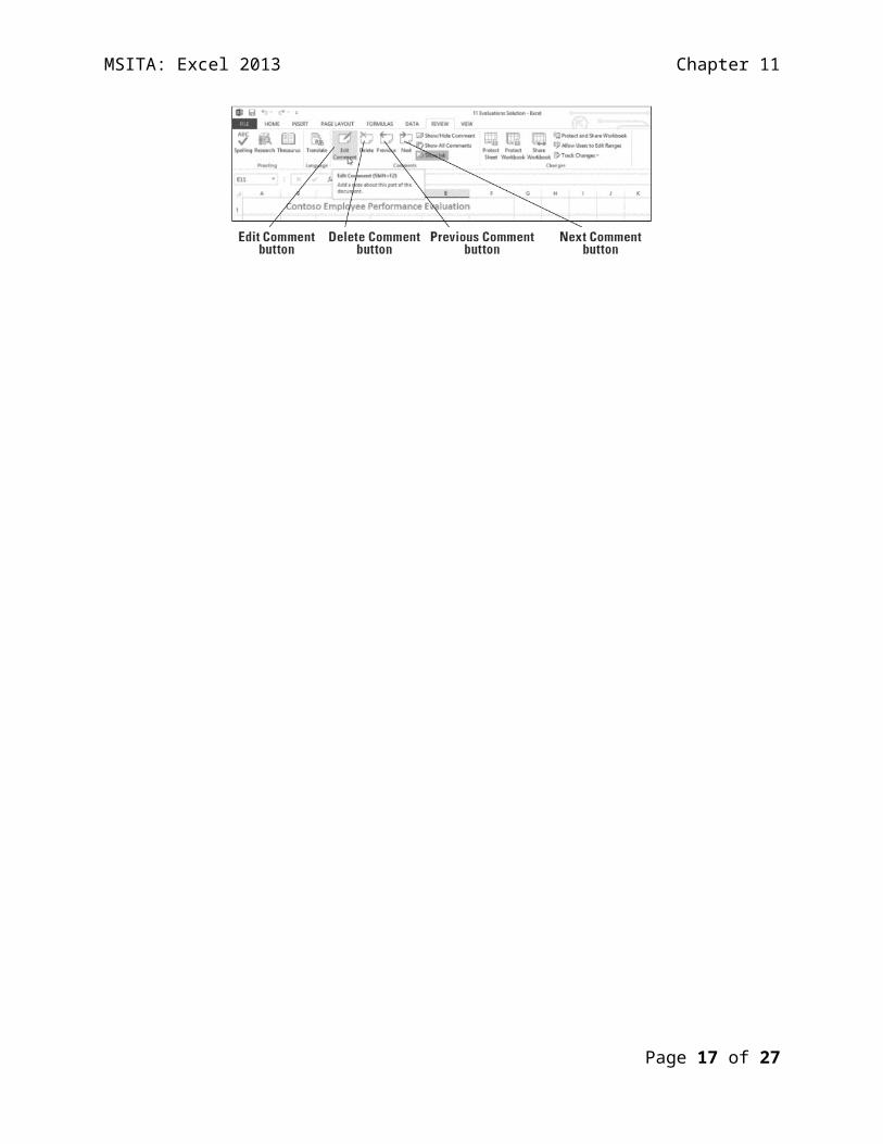
Step-by-Step 19 – Edit a CommentGET READY. USE the workbook from the previous exercise.1. Click cell E11 and move the mouse pointer to the Edit Comment button on the REVIEW tab. The ScreenTip also shows Shift + F2 as an option, as shown in Figure 11-24.

of 18


2. Click the Edit Comment button.3. Following the existing comment text, type a .(period) followed by a space and then Placed on probation. Then click any cell between F4 and D8.4. Click Next. The comment in D8 is displayed.5. Select the existing comment text in D8 and type MA completed; can now prescribe medications.6. Click cell E4 and click Edit Comment.7. Select the text in the comment attached to E4. On the HOME tab, click Bold.8. Click cell E11, click the REVIEW tab, and click Edit Comment.9. Select the name and the comment text. Click the HOME tab and notice that the Fill Color and Font Color options are dimmed. Right-click on the selected text and select Format Comment.10. In the Format Comment dialog box, click the arrow in the Color box and click Red. Click OK to apply the format and close the dialog box. There is no fill option for the comment box.PAUSE. SAVE the workbook and LEAVE it open for the next exercise.

Step-by-Step 20 – Delete a CommentGET READY. USE the workbook from the previous exercise.1. Click cell E4. The comment for this cell is displayed.2. On the REVIEW tab, in the Comments group, click Delete.PAUSE. SAVE the workbook and LEAVE it open for the next exercise.

Step-by-Step 21 – Print Comments in a WorkbookGET READY. USE the workbook from the previous exercise.1. On the REVIEW tab, click Show All Comments. Notice that the comments slightly overlap each other.2. In cell D8, click the border of the comment box. Select the center sizing handle at the bottom of the box and drag upward until the comment in cell E11 is completely visible.3. Move the mouse pointer until it is a four-headed arrow on the border of the comment in cell F10. Drag the comment so it no longer overlaps the comment in cell E11 (see Figure 11-25).4. Click the PAGE LAYOUT tab, and in the Page Setup group, click Orientation. Click Landscape.5. In the Page Setup group, click the Page Setup dialog box launcher.6. On the Sheet tab, in the Comments box, click As displayed on sheet.7. Click Print Preview. The Print Options window in Backstage opens.8. Click Print.9. SAVE and CLOSE the workbook.CLOSE Excel.

of 18


Competency Assessment

Project 11-1: Protect a File with a PasswordIn this project, the office manager has asked you to create an inventory of company credit cards and save the file with a password.

GET READY. LAUNCH Excel if it is not already open.1. Open a Blank workbook and type Contoso Credit Card Inventory in cell A1.2. Type and format the information in the figure below. The title in cell A1 is merged and centered, with Cell Style Heading 1 applied. The labels in row 3 are centered, with Cell Style Heading 3 applied.

3. SAVE the file as 11 Credit Cards Solution for use in each of the other exercises.4. Click the FILE tab and Info is automatically selected; click Protect Workbook and choose Encrypt with Password.5. In the Encrypt Document dialog box, type 11P1!s5 and reenter the same password in the Confirm Password dialog box.6. SAVE and CLOSE the workbook.LEAVE Excel open for the next project.

of 18


Project 11-2: Email and Save a File to SkyDriveIn this project, you will email your workbook to your instructor and save the file to the SkyDrive.

GET READY. LAUNCH Excel if it is not already open.1. OPEN the 11 Credit Cards Solution file you created in the first project. Use the password you created in Project 11-1.2. SAVE the file as 11 Credit Cards Email Solution.3. Select the FILE tab, and then Share.4. Invite People is already selected. Click Save to Cloud.5. Click on your SkyDrive icon and then Browse, and select the SkyDrive folder for this lesson.6. Click Save. You return to the Share screen.7. Type the [email address of your instructor], in the personal message box, type Project2 Assignment and click the Share button SEND the email message.CLOSE the workbook and LEAVE Excel open for the next project.

Proficiency Assessments

Project 11-3: Send Links for Editing and Viewing a File on the WebIn this project, you will send the links for viewing and editing the file on the Web to your instructor and yourself.

GET READY. LAUNCH Excel if it is not already open.1. OPEN the 11 Credit Cards Solution file you created in the first project. Use the password you created in Project 11-1.2. SAVE the file as 11 Credit Cards Links Solution.3. Use the Share option on the Backstage view to save the file to the cloud.4. Open your email program and add your instructor’s email address. In the body of the message, type View and press Enter and then type Edit.5. Return to Excel’s Backstage view Share page and click Get a Sharing Link for viewing, copy this in the email message after the word View, and then copy the link for editing and copy this in the email message after the word Edit. SEND the email message.6. SAVE and CLOSE all open workbooks.LEAVE Excel open for the next project.

of 18


Project 11-4: Add Comments to a FileIn this project, you will add comments to a file.

GET READY. LAUNCH Excel if it is not already open.1. OPEN the 11 Credit Cards Solution file you created in the first project. Use the password you created in Project 11-1.2. SAVE the file as 11 Credit Cards Comments Solution.3. In cell B4, type a new comment Initial E will be removed on next card.4. In cell D9, type a new comment Card lost – need to cancel if not found by tomorrow.5. In cell B12, type a new comment Yossi will be leaving at the end of the quarter – make sure to cancel card.6. Edit the comment in D9 to just say Card lost and found [today’s date].7. Make sure all comments are hidden.8. PRINT the worksheet with the comments displayed at the end of the sheet.9. SAVE and CLOSE the workbook.LEAVE Excel open for the next project.

of 18


Mastery Assessments

Project 11-5: Track ChangesIn this project, you will open the credit card file and track changes with different users.

GET READY. LAUNCH Excel if it is not already open.1. OPEN the 11 Credit Cards Solution file you created in the first project. Use the password you created in Project 11-1.2. SAVE the file as 11 Credit Cards Changes Solution.3. In cell F3, type Balance and continue the formatting for row 3.4. Format column F to be Accounting Number Format.5. Change the label in row 1 to be merged and centered across A1:F1.6. Track changes for all users.7. Change the username prior to each change to be the user whose name is on the card in row 4 and enter the balances below for each user in column F. SAVE the workbook after each balance is entered.

Jenny E. Geist $3,533.15Cassie A. Hicks $9,929.25Dan A. Wilson $952.92Mor O. Hezi $9,768.55Nicole I. Holliday $1,669.72Rebecca E. Laszlo $166.00Srinivas R. Iragavarapu $6,186.08Stephanie T. Bourne $8,662.97Yossi O. Banai $1,621.48

8. List the changes on a new sheet.9. Create a copy of the History sheet to a new workbook and save the workbook as 11 Credit User Changes Solution.10. Accept everyone’s changes except Dan’s in F6 and Rebecca’s in F9.11. SAVE and CLOSE both workbooks.LEAVE Excel open for the next project.

Project 11-6: Lock Cells and Protect Worksheet ElementsThis project will put together various features of worksheet security and annotation, and then have you share the workbook with other users.

GET READY. LAUNCH Excel if it is not already open.1. OPEN the 11 Credit Cards Solution file you created in the first project. Use the password you created in Project 11-1.

of 18


2. SAVE the file as 11 Credit Cards Passwords Solution.3. Turn off the password for the file (delete all characters).4. Add a label in F3: Birthday and one in G3: Mom Name. Format these two labels the same as other labels in the row and increase column width to fit.5. Change the title of the workbook in A1 to read Contoso Credit Card Passwords and center across A1:G1.6. Add a label in A17: Password is Birthday in yyyymmdd format + first 4 characters of Mom’s Maiden name.7. Unlock the input for Birthday and Mom Name columns (F4:G12).8. Protect Sheet with the password of the company name: Contoso.9. Send this workbook in an email to your instructor. The subject should read: CC Passwords. The body text should read Go to your row. In column F type your birth date. In column G type your mother’s maiden name. After you complete these changes, make sure to email the workbook back to me on Friday.10. The following will simulate getting each workbook back. Enter the following data:

Name on Card Birthday Mom NameJenny E. Giest 4/7/1955 SoonCassie A. Hicks 11/6/1953 BantiDan A. Wilson 11/27/1949 MeadowsMor O. Hezi 5/27/1950 MayoNicole I. Holliday 7/20/1952 KimRebecca E. Laszlo 2/23/1970 UntchSrinivas R. Iragavarapu 2/1/1959 ChiaStephanie T. Bourne 6/10/1945 BrauningerYossi O. Banai 7/5/1948 Posti

11. In the Excel Options dialog box, change the User name to the original name for this computer.12. Put a comment in cell G4: Password would look like 19550407Soon.13. Click the FILE tab, choose Options, select Quick Access Toolbar, click the Reset button, and select the Reset all customizations option to return your Excel settings to normal.14. Send an email to your instructor with a critique of this worksheet. In the email text, tell your instructor how you would improve the worksheet or the process of creating it.CLOSE Excel.

of 18

Step-by-Step 1 – Protect a Web viewStep-by-Step 3 – Allow Multiple Users to Edit a...

Documents

Transcript of Step-by-Step 1 – Protect a Web viewStep-by-Step 3 – Allow Multiple Users to Edit a...