Statistik for bioteknik SF1911 CBIOT3Forelasning 9: Modellbaserad data-analys

Timo Koski

TK

21.11.2017

Larandemal

I Konfidensintervall for vantevardet i N (µ, σ2).i) σ kantii) σ okant –¿ t-fordelning

I Konfidensintervall for u1 − µ2 med N (µ1, σ21 ), N (µ2, σ2

2 ).i) σ1 = σ2 kanda, σ1 = σ2 okandaii) σ1 6= σ2 okanda

I Bootstrap

Estimating a Population Mean

Now we consider the task of estimating a population mean. Theseare questions like

I What is the mean amount milk obtained from cows in Skanein 2016? (Existing population)

Here we think of proceeding by observing the amount of milkproduced by cows in a randomly chosen sub-population of farms inSkane (sample).

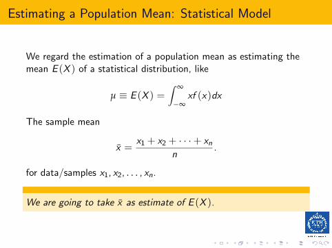
Estimating a Population Mean: Statistical Model

We regard the estimation of a population mean as estimating themean E (X ) of a statistical distribution, like

µ ≡ E (X ) =∫ ∞

−∞xf (x)dx

The sample mean

x =x1 + x2 + · · ·+ xn

n.

for data/samples x1, x2, . . . , xn.

We are going to take x as estimate of E (X ).

Estimating a Population Mean: Law of Large Numbers

We are going to take x as estimate of µ(= E (X ). Why ?

X1,X2, . . . ,Xn are independent have the same distribution(=equally distributed) with mean µ och standard deviation σ. If nis very large we have

The Law of Large Numbers

X =1

n

n

∑i=1

Xi ≈ µ

where µ is the common mean of X1,X2, . . . ,Xn, . . .

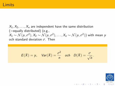
Limits

X1,X2, . . . ,Xn are independent have the same distribution(=equally distributed) (e.g.,X1 ∼ N (µ, σ2),X2 ∼ N (µ, σ2), . . . ,Xn ∼ N (µ, σ2)) with mean µoch standard deviation σ. Then

E (X ) = µ, Var(X ) =σ2

noch D(X ) =

σ√n

.

Law of Large Numbers

X1,X2, . . . ,Xn are independent have the same distribution(=equally distributed) with mean µ och standard deviation σ.If n is very large we have

The Law of Large Numbers

X =1

n

n

∑i=1

Xi ≈ µ

where µ is the common mean of X1,X2, . . . ,Xn, . . .This is because

Var(X ) =σ2

n→ 0

as n→ ∞

We are going to take x as estimate of µ. Why ?

By the Law of Large Numbers x is close to the true value µ !There is no systematic error (a.k.a. bias) either, since E (X ) = µ.

X1,X2, . . . ,Xn are all N (µ, σ2), then x is the maximum likelihoodestimate of µ, too. (Details omitted).

Estimating a Population Mean

We are going to follow the same general procedure as above, i.e,

I Find the critical value for chosen level of confidence α.

I Find the margin of error E

I Form the confidence interval (confidence level 1− α)

x − E < µ < x + E

Estimating a Population Mean: the critical value

When finding the critical value we have to consider two cases (a)and (b):

(a) σ =√

Var(X ) =√∫ ∞

−∞(x − E (X ))2f (x)dx is known

(b) σ is not known

Estimating a Population Mean (a) : the critical value whenσ known

The critical value λα/2 is found as in estimation of populationproportion.

Estimating a Population Mean (a)

This is justified by the central limit theorem applied to arithmeticmean

X approximatively ∼ N(µ, σ2/n

)Or, with with the cumulative density Φ(x)

P(a < X ≤ b) ≈ Φ(b− µ

σ/√n

)−Φ

(a− µ

σ/√n

)

Z Score

Therefore the population Z Score is standard normal

Z =X − µ

σ/√n∼ N(0, 1)

and we have for Z the same picture as above.

Critical value: read zα/2 as λα/2

Estimating a Population Mean (a): σ known

We can therefore to follow exactly the same procedure as above,i.e,

I Find the critical value λα/2 for chosen level of confidence1− α.

I Find the margin of error E

I Form the confidence interval (confidence level 1− α)

x − E < µ < x + E

Estimating a Population Mean (a): the margin of error

When σ is known, the margin of error E is

Edef= λα/2

σ√n

This reflects the fact that σ√n

is standard deviation in N(µ, σ2/n

).

The confidence interval (a): σ is known

Confidence Interval or the Interval Estimate for thepopulation mean µ

x − E < µ < x + E , where E = λα/2σ√n

Other equivalent expressions are

x ± E

or(x − E , x + E )

Confidence Interval or the Interval Estimate for thepopulation mean µ

Langden av intervallet

x − λα/2σ√n< µ < x + λα/2

σ√n

,

ar = 2 · λα/2σ√n

.

I Intervallet blir kortare med mer data (storre n) for givet α.

I Intervallet blir bredare med storre 1− α (via storre λα/2) forgivet n: storre konfidensgrad men en oprecisare skattning.

Interpretation of the CI: Correct

Suppose we have, with α = 0.05 and some data, obtained by theprocedure above 98.08 < µ < 98.32

We are 95 % confident that the interval with endpoints 98.08 and98.32 contain the true value of µ.

Interpretation of the CI: Correct

This means that if we were to select many different samples of thesame size and construct the corresponding CIs, 95 % of themwould actually contain the value of the population proportion µ. Inthis correct interpretation 95% refers to the success rate of the

process being used to estimate the mean.

Interpretation of the CI: Wrong !

Because µ is a fixed constant (but unknown) it would be wrong tosay that ” there is a 95% chance that µ will fall between 98.08 and98.32 ”. The CI does not describe the behaviour of individualsample values, so it would be wrong to say that ” 95% of all datavalues fall between 98.08 and 98.32 ”. The CI does not describethe behaviour of individual sample means, so it would also bewrong to say that ” 95% of sample means fall between 98.08 and98.32 ”.

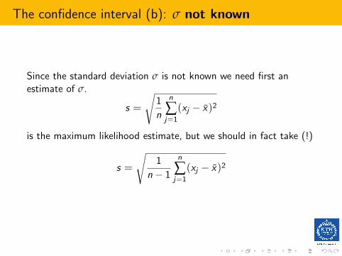
The confidence interval (b): σ not known

Since the standard deviation σ is not known we need first anestimate of σ.

s =

√1

n

n

∑j=1

(xj − x)2

is the maximum likelihood estimate, but we should in fact take (!)

s =

√1

n− 1

n

∑j=1

(xj − x)2

t score

If s =√

1n−1 ∑n

j=1(xj − x)2, then we have the following:

The distribution of

t =x − µ

s√n

is a t-distribution with n− 1 degrees of freedom .

t-distribution : Degrees of freedom ??

The number of degrees of freedom is the number of samplevalues that can vary after certain restrictions have been imposedon all data values

For example, if x =x1 + x2 + · · ·+ xn

n= 5 is imposed, we can

vary, e.g., x1, x2, . . . , xn − 1, but xn must be chosen so that x isequal to 5. Hence the degree of freedom is n− 1.

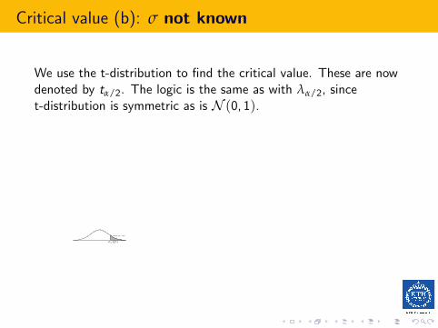
Critical value (b): σ not known

We use the t-distribution to find the critical value. These are nowdenoted by tα/2. The logic is the same as with λα/2, sincet-distribution is symmetric as is N (0, 1).

area=α

tα(f)

t-distribution

The density curves for N (0, 1) (blue) and t with four degrees of

freedom (green)−5 −4 −3 −2 −1 0 1 2 3 4 50

0.05

0.1

0.15

0.2

0.25

0.3

0.35

0.4

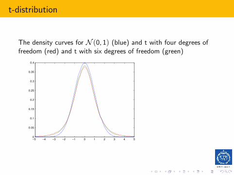
t-distribution

The density curves for N (0, 1) (blue) and t with four degrees offreedom (red) and t with six degrees of freedom (green)

−5 −4 −3 −2 −1 0 1 2 3 4 50

0.05

0.1

0.15

0.2

0.25

0.3

0.35

0.4

Critical value

Here we find tα for various values of α and f =degrees of freedom.f α 0.10 0.05 0.025 0.01 0.005 0.001 0.00051 3.08 6.31 12.71 31.82 63.66 318.31 636.622 1.89 2.92 4.30 6.96 9.92 22.33 31.603 1.64 2.35 3.18 4.54 5.84 10.21 12.924 1.53 2.13 2.78 3.75 4.60 7.17 8.615 1.48 2.02 2.57 3.36 4.03 5.89 6.87

For example t0.05 = 2.02 for 5 degrees of freedom.

Estimating a Population Mean: the margin of error (b)

When σ is not known, the margin of error E is

Edef= tα/2

s√n

where tα/2 has n− 1 degrees of freedom.

The confidence interval: σ not known

Confidence Interval or the Interval Estimate for thepopulation mean µ σ not known

x − E < µ < x + E , where E = tα/2s√n

orx ± E

or(x − E , x + E )

Tva stickprov, konfidensintervall for skillnad mellanvantevarden.

a) σ1 och σ2 kanda

Vi vill nu skaffa oss ett konfidensintervall for µ1 − µ2. En naturligskattning av µ1 − µ2 ar X − Y . Eftersom den ar enlinjarkombination av oberoende normalfordelade variabler, sa galleratt

(X − Y )− (µ1 − µ2)√σ21n1

+σ22n2

ar N (0, 1)-fordelad.

Tva stickprov, konfidensintervall for skillnad mellanvantevarden.

Av detta leds vi till

Iµ1−µ2 = x − y ± λα/2

√σ21

n1+

σ22

n2.

Om σ1 = σ2 = σ reduceras detta till att

(X − Y )− (µ1 − µ2)

σ√

1n1

+ 1n2

ar N (0, 1)-fordelad och

Iµ1−µ2 = x − y ± λα/2σ

√1

n1+

1

n2.

Tva stickprov, konfidensintervall for skillnad mellanvantevarden.

b)σ1 = σ2 = σ okand

Vi betraktar nu fallet da σ1 = σ2 = σ, men dar σ ar okand. Dettaskattas med s dar s2 ar den sammanvagda stickprovsvariansen.Man kan visa att man skall valja

s2 =(n1 − 1)s21 + (n2 − 1)s22

n1 + n2 − 2

och att(X − Y )− (µ1 − µ2)

S√

1n1

+ 1n2

ar t(n1 + n2 − 2)-fordelad.

Tva stickprov, konfidensintervall for skillnad mellanvantevarden.

Vi far

Iµ1−µ2 = x − y ± tα/2(n1 + n2 − 2)s

√1

n1+

1

n2.

Sammanfattning (1)

Sats

Lat x1, . . . , xn1 och y1, . . . , yn2 vara slumpmassiga, av varandraoberoende stickprov fran N(µ1, σ2

1 ) respektive N(µ2, σ22 ).

Om σ1 och σ2 ar kanda sa ar

Iµ1−µ2 = (x − y − λα/2D, x − y + λα/2D)

ett tvasidigt konfidensintervall for µ1 − µ2 med konfidensgraden

1− α; har ar D =√

σ21/n1 + σ2

2/n2.

Sammanfattning

Sats

Om σ1 = σ2 = σ dar σ ar okant sa ar

Iµ1−µ2 = (x − y − tα/2(f )d , x − y + tα/2(f )d)

ett tvasidigt konfidensintervall for µ1 − µ2 med konfidensgraden1− α; har ar d = s

√1/n1 + 1/n2 dar f = (n1 − 1) + (n2 − 1).

Two samples = Tva stickprov

In an experiment designed to test the effectiviness of paroxetine fortreating bipolar depression, subjects were measured using theHamilton Depression scale with results as follows:

Placebo group n1 = 43 x = 21.57, s1 = 3.87Paroxenite treatment group n2 = 33 y = 20.38, s2 = 3.91

Two samples

We assume that we have independent samples and normaldistributions. We must assume this, we have just summaries ofdata, no chance of looking at histograms or boxplots.We insert data in pooling (sammanvagning)

s2 =(n1 − 1)s21 + (n2 − 1)s22

n1 + n2 − 2=

(43− 1) · 3.872 + (33− 1) · 3.912

43 + 33− 2

= 15.11

We choose α = 0.05. The quantiles are found from thet-distribution with 43 + 33− 2 = 74 degrees of freedom. Thisgives us t0.025 = 1.993 (by >>tinv(0.975, 74) in Matlab).

Two samples; the confidence interval computed

s2 =(43− 1) · 3.872 + (33− 1) · 3.912

43 + 33− 2= 15.11

t0.025(74) = 1.993

Iµ1−µ2 = x − y ± tα/2(n1 + n2 − 2)s

√1

n1+

1

n2

= (21.57− 20.38)± 1.993 ·√

15.11 ·√

1

43+

1

33

= 1.19± 1.7930 = [−0.603, 2.938]

Tva stickprov for paroxetine; Konfidensintervall medkonfidens grad 0.95

Iµ1−µ2 = [−0.603, 2.938]

Men vad sager detta for oss ? Vilken kunskap om paroxetine harde givna data gett oss i form av detta konfidensintervall?

Vi kommer att fa ett svar med hjalp av teorin om hypotesprovning.Men forst ett fall till.

t-distribution

The derivation of the t-distribution wasfirst published in 1908 by William Sealy Gosset, while he worked ata Guinness Brewery in Dublin. He was prohibited from publishingunder his own name, so the paper was written under thepseudonym Student.

Bootstrap: dictionary

(1) Loop of leather or cloth sewn at the top rear, or sometimes oneach side, of a boot to facilitate pulling it on. (2) a means ofadvancing oneself or accomplishing something relying entirely on

one’s efforts and resources.

Bootstrap

Namnet bootstrap (pa sv. stovelstropp) harstammar fran uttrycketi amerikansk engelska pull oneself up by the bootstraps, vilketbetyder att man forbattrar ens (ekonomiska/sociala o.s.v.)situation genom egna insatser utan andras hjalp. Ett uttryck medlikadan betydelse ar att lyfta sig sjalv i haret (jfr. baron vonMunchausens aventyr).

Bootstrap

Atersampling: Vi lottar fram ett forsta fiktivt eller bootstrap-stickprov ur vara matdata genom att pa mafa dra n st medaterlaggning fran x1, . . . , xn.Detta stickprov blir typiskt ungefar som det ursprungliga aven omvissa observationer saknas och vissa finns i dubbel eller kansketredubbel uppsattning.

Bootstrap med matlab: exempel

Vi har, till exempel,

x1 = −0.2746, x2 = −1.1730, x3 = 1.4842, x4 = 1.1454, x5 = −1.6248,

x6 = 0.9985, x7 = 0.4571, x8 = −1.2315, x9 = 0.9868, x10 = −0.5941

eller

x = [ −0.2746 −1.1730 1.4842 1.1454 −1.62480.9985 0.4571 −1.2315 0.9868 −0.5941];

Matlabkommandot unidrnd(10,1,10) ger tio slumptal ur denlikformiga fordelningen pa de tio heltalen i 1, . . . , 10, d.v.sp(i) = 1/10.>> z=unidrnd(10,1,10)z =5 1 6 3 2 5 6 3 7 10Bootstrapstickprovet ges nu av >> bssampl=x(z)

Bootstrap med matlab: exempel

Med >> bssampl=x(z)fas bootstrap stickprovetbssampl =Columns 1 through 7-1.6248 -0.2746 0.9985 1.4842 -1.1730 -1.6248 0.9985Columns 8 through 101.4842 0.4571 -0.5941

Medelfel for en skattning & bootstrap

Ur detta nya stickprov beraknar vi skattningen θ1,obs av enparameter θ. Detta upprepas nu B ganger (kanske B = 1000 ellerB = 10000) och ur dessa B fiktiva stickprov far vi B skattningarθ1,obs, θ2,obs, . . . , θB,obs. Vi far da en medelfelsskattning genom attberakna spridningen av dessa d.v.s.

d(θ) =

√√√√ 1

B − 1

B

∑i=1

(θi ,obs − θmedel,obs)2

dar θmedel,obs = ∑B1 θi ,obs/B ar aritmetiska medelvardet av de B

skattningarna for de B fiktiva stickproven.

Medelfel for en skattning & bootstrap

Vi hade simulerat sa att

x = [ −0.2746 −1.1730 1.4842 1.1454 −1.62480.9985 0.4571 −1.2315 0.9868 −0.5941];

ar tio oberoende stickprov pa Xi ∼ N (0, 1). Vi har attθ = 1

10 (X1 + . . . + X10) ∈ N (0, 110 ). Om vi drar B

bootstrap-stickprov fran x och beraknar x i ,obs for i = 1, . . . ,B, far

vi enligt receptet ovan en bootstrap-skattning av√

110 = 0.3162. I

figuren ses histogrammet for x i ,obs for i = 1, . . . ,B medB = 1000, dar standardavvikelsen ar d(θ∗) = 0.339.

Medelfel for en skattning & bootstrap

I figuren ses histogrammet for x i ,obs for i = 1, . . . ,B medB = 1000, dar standaravvikelsen ar 0.339.

−1.5 −1 −0.5 0 0.5 10

50

100

150

200

250

Medelfel for en skattning & bootstrap

De fiktiva stickproven ar framlottade enligt den empiriskafordelningen som lagger massan 1/n i vardera av de nobservationerna. Denna empiriska fordelning ar en skattning av densanna fordelningen F som observationerna genererats av. Vi hardarmed lyckats skapa en kopia av det ursprungliga forsoket (darvara data kom fran F ). Vi kan da undersoka egenskaper hos denursprungliga skattningen genom undersoka skattningen i kopian.

Luria & Delbruck

X ∼ Poi(λ), E (X ) = λ, Var(X ) = λ.

I Simulera x = 100 stickprov fran, t.ex., Poi(0.2)(poissrnd(0,2,1,100)).

I Atersampla x , x∗i , i = 1, . . . ,B, t.ex. B =10 000 ggr. x∗i =stovelstropp(x).

I Berakna x∗i och std(x∗i ) for varje x∗iI Berakna kvoten varians/medelvarde, qi = std2(x∗i ))/x

∗i for

i = 1, . . . ,B.

I Ta fram histogram for qina, mean(q) och std(q).

Luria & Delbruck

X ∼ Poi(λ), E (X ) = λ, Var(X ) = λ ⇒ Var(X )/E (X ) = 1.

I Histogram for qina, mean(q) och std(q).

I Det finns ingen matematisk formel for fordelningen av kvotenqi = std2(x∗i ))/x

∗i . mean(q) = 1.0299, std(q)= 0.1164.

0.7 0.8 0.9 1 1.1 1.2 1.3 1.4 1.5 1.6

0

500

1000

1500

2000

2500

3000

Bilaga: Bootstrap stovelstropp.m

function bssampl=stovelstropp(x)% atersamplar datat i x med likformig sannolikhet (unirnd ochger bssampl som ett bootstrap %stickprov. m=length(x);z=unidrnd(m,1,m);bssampl=x(z);