Statistical Methods for Nitrate Vulnerable Zone Review...
81
Report Reference: UC10943.07 November 2015 Statistical Methods for Nitrate Vulnerable Zone Review 2017
Transcript of Statistical Methods for Nitrate Vulnerable Zone Review...
Report Reference: UC10943.07
November 2015
Statistical Methods for Nitrate Vulnerable
Zone Review 2017

RESTRICTION: This report has the following limited distribution:
External: Environment Agency
Any enquiries relating to this report should be referred to the Project Manager at the
following address:
WRc plc,
Frankland Road, Blagrove,
Swindon, Wiltshire, SN5 8YF
Telephone: + 44 (0) 1793 865000
Website: www.wrcplc.co.uk
Follow Us:
WRc is an Independent Centre
of Excellence for Innovation and
Growth. We bring a shared
purpose of discovering and
delivering new and exciting
solutions that enable our clients
to meet the challenges of the
future. We operate across the
Water, Environment, Gas, Waste
and Resources sectors.

© Environment Agency 2015 The contents of this document are subject to copyright and all rights are reserved. No part of this document may be reproduced, stored in a retrieval system or transmitted, in any form or by any means electronic, mechanical, photocopying, recording or otherwise, without the prior written consent of Environment Agency.
This document has been produced by WRc plc.
Statistical Methods for Nitrate Vulnerable Zone
Review 2017
Authors:
Vicki Bewes
Project Statistician
Catchment Management
Date: November 2015
Report Reference: UC10943.07
Andrew Davey
Senior Statistician
Catchment Management
Project Manager: Rob Stapleton
Project No.: 16426-0
Alice Goudie
Database Analyst
Catchment Management
Client: Environment Agency
Client Manager: Stephanie Cole
Alastair Halliday
Statistician
Catchment Management

Document History
Version
number
Purpose Issued by Quality Checks
Approved by
Date
V0.1 Interim report to confirm data processing. Andrew Davey NA 12/06/15
V0.2 Draft report to confirm statistical methodology and QA procedures
Andrew Davey
Rob Stapleton 03/07/15
V0.3 Draft report addressing EA comments on V0.2 and including kriging analysis
Rob Stapleton Rob Stapleton 24/07/15
V0.4 Draft final report addressing EA comments on V0.2 and V0.3 Rob Stapleton Rob Stapleton 04/08/15
V0.5 Final report addressing EA comments on V0.4 Rob Stapleton Rob Stapleton 27/08/15
V0.6 Inclusion of metadata appendix for SQL database and geodatabase
Rob Stapleton Rob Stapleton 24/09/15
V0.7 Amended final report with updated kriging results and Appendix C
Andrew Davey Rob Stapleton 26/11/15

Contents
Glossary ................................................................................................................................... 1
Executive Summary ................................................................................................................. 4
1. Introduction .................................................................................................................. 5
1.1 Background ................................................................................................................. 5
1.2 Objectives .................................................................................................................... 5
1.3 Structure of this report ................................................................................................. 6
2. Surface water methodology ........................................................................................ 7
2.1 Source datasets .......................................................................................................... 7
2.2 Data processing .......................................................................................................... 9
2.3 Data analysis methods .............................................................................................. 14
3. Groundwater methodology ........................................................................................ 23
3.1 Source datasets ........................................................................................................ 23
3.2 Data processing ........................................................................................................ 25
3.3 Data analysis methods .............................................................................................. 29
3.4 Kriging ....................................................................................................................... 45
4. Recommendations .................................................................................................... 54
References ............................................................................................................................. 55
Appendices
Appendix A Multiple Outlier Test................................................................................. 56
Appendix B Meta Data Overview ................................................................................ 59
Appendix C Evaluation of alternative kriging models .................................................. 71

List of Tables
Table 2.1 Purpose codes included in surface water analysis ................................... 7
Table 2.2 Summary of water company surface water dataset .................................. 9
Table 2.3 Sampling point types included in surface water analysis ........................ 10
Table 2.4 Summary of surface water data processing ............................................ 13
Table 2.5 Summary of confidence classes .............................................................. 14
Table 2.6 Minimum data rules for surface water analysis ....................................... 15
Table 2.7 Summary of surface water methodological refinements ......................... 21
Table 3.1 Purpose codes included in groundwater dataset .................................... 23
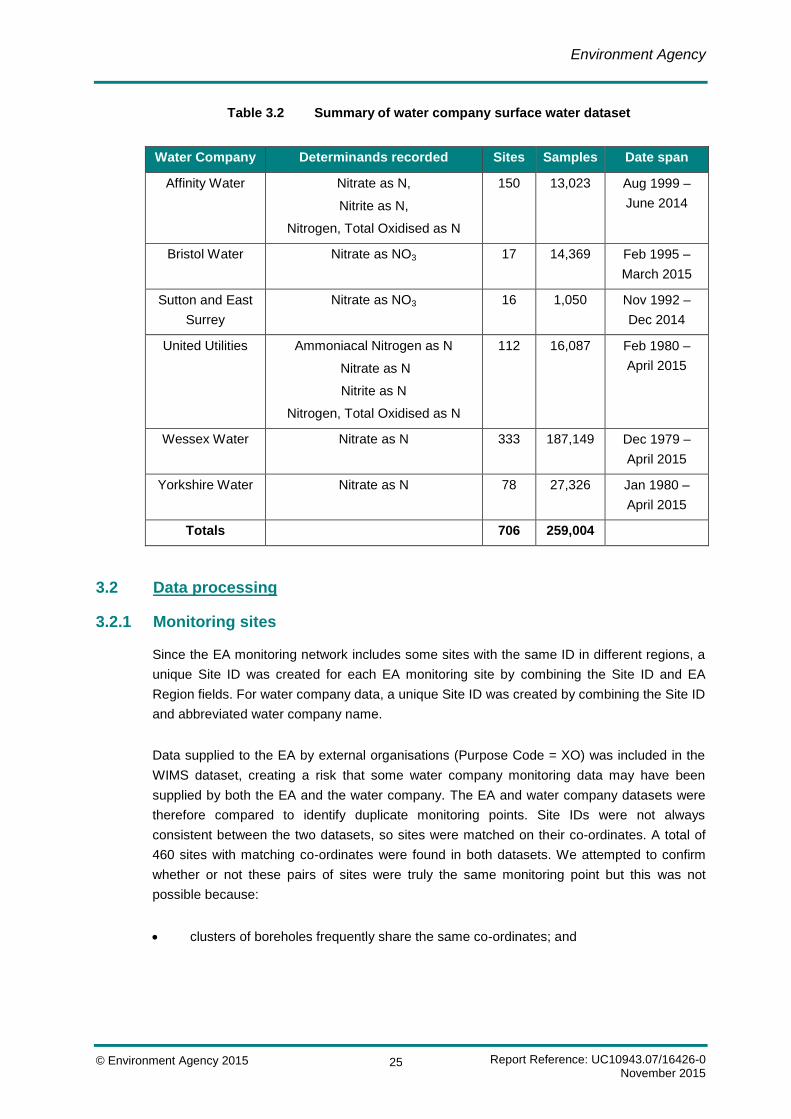
Table 3.2 Summary of water company surface water dataset ................................ 25
Table 3.3 Sampling point types included in groundwater analysis.......................... 27
Table 3.4 Summary of groundwater data processing ............................................. 29
Table 3.5 Minimum data rules for groundwater analysis ......................................... 31
Table 3.6 Summary of groundwater methodological refinements ........................... 42
Table 3.7 Parameter estimates for current and future concentration variogram models .................................................................................... 49
Table A.1 Critical values (P = 1%) of the tmax statistic ............................................. 57
Table B.1 Metadata containing descriptions for each SQL database table contained within the SW and GW SQL Server Database ................................................................................................. 59
Table B.2 Metadata containing descriptions and a summary/purpose for each Geodatabase Table included in the final File Geodatabase ........................................................................................... 61
Table B.3 Metadata containing descriptions and a summary/purpose for each Geodatabase feature class included in the final File Geodatabase ........................................................................................... 66
Table C.1 Comparative kriging performance of alternative variogram models ..................................................................................................... 72
List of Figures
Figure 2.1 Historical trend and future forecast of 95th percentile nitrate
concentration using quantile regression, and comparison to the 11.29 mg N/l (50 mg NO3/l) standard (red dashed line) .................... 20
Figure 3.1 Historical trend and future forecast of mean nitrate concentration using AntB, and comparison to the 9.71 mg N/l (43 mg NO3/l) standard (horizontal blue dashed line) ........................ 36
Figure 3.2 Historical trend and future forecast of mean nitrate concentration using AntC, and comparison to the 9.71 mg N/l (43 mg NO3/l) standard (horizontal blue dashed line) ........................ 39
Figure 3.3 Historical trend and future forecast of mean nitrate concentration using the ‘Mean Concentration’ method, and
comparison to the 9.71 mg N/l (43 mg NO3/l) standard (horizontal blue dashed line) ................................................................... 41
Figure 3.4 Location of the 4,160 groundwater monitoring points used in the kriging analysis .................................................................................. 48
Figure 3.5 Variogram for current (a) and future (b) 95th percentile TIN concentrations ......................................................................................... 51
Figure 3.6 Kriged predictions of current (2015) 95th percentile TIN
concentration ........................................................................................... 52
Figure 3.7 Kriged predictions of future (2027) 95th percentile TIN
concentration ........................................................................................... 53
Figure C.1 Comparison of observed and predicted nitrate concentrations ......................................................................................... 73

Environment Agency
Report Reference: UC10943.07/16426-0 November 2015
© Environment Agency 2015 1
Glossary
Autocorrelation Autocorrelation describes the tendency for observations in a
sequence to be correlated with preceding observations. The strength
of correlation between successive pairs of measurements is quantified
by a lag-1 autocorrelation coefficient, which takes values between -1
(perfect negative correlation) and +1 (perfect positive correlation).
Positive autocorrelation is common in water quality monitoring data,
where the measured concentration in one sample often gives a good
idea of what the measured concentration will be in the next sample
Bimodal distribution The spread of concentration values in a set of water quality samples
commonly has a single peak (or ‘mode’), with the bulk of samples
having intermediate values and a relatively low number of samples
having low or high values. Some datasets, however, show a spread of
values with two peaks - a cluster of lower concentrations and a
second cluster of higher concentrations; this is termed a bimodal
distribution.
A bimodal distribution can indicate strongly fluctuating water quality, or
indicate that water samples have been collected from two locations
with different levels of pollution.
Coefficient of variation (CoV) A standardised measure of the degree of variability in a dataset,
relative to the mean value of the dataset. The CoV is calculated by
dividing the mean by the standard deviation. Monitoring points with
higher mean concentrations tend also to show higher variability in
concentrations, so the CoV provides a way of comparing variability
among monitoring locations with different levels of pollution.

Environment Agency
Report Reference: UC10943.07/16426-0 November 2015
© Environment Agency 2015 2
Confidence interval / limits A confidence interval quantifies uncertainty in the estimate of a
parameter by giving a range of values that is likely to include the true
(unknown) population parameter. For example, a 90% confidence
interval around a sample mean indicates that one can be 90%
confident that the true population mean lies within that range. In other
words, there is a probability of only 10% or 0.1 that the true mean
value lies outside the stated confidence interval.
The upper and lower bounds of the confidence interval are called
confidence limits.
Kriging Kriging is a statistical interpolation technique. It is used to predict the
value of a function at a given point by computing a weighted average
of the known values of the function in the neighbourhood of the point
(i.e. predict TIN concentrations at unmonitored locations, based on
TIN concentrations at monitored locations). The closer the monitoring
point is to the location for which concentrations are to be predicted,
the greater the weight given to the monitoring point.
(Arithmetic) Mean This is a measure of the central tendency or ‘middle’ value of a
dataset. It is the sum of the data values divided by the number of
observations.
Monte Carlo simulation Monte Carlo methods are a broad class of computational algorithms
that rely on repeated random sampling to simulate a situation and
obtain numerical results; typically a simulation is run many times over
in order to obtain the probability distribution of an unknown parameter.
The name comes from the resemblance of the technique to the act of
playing and recording results in a real gambling casino. Monte Carlo
methods are often used in physical and mathematical problems when
it is difficult or impossible to obtain a closed-form expression, or
unfeasible to apply a deterministic algorithm.
MOT Short for Multiple Outlier Test. By definition, outliers are not
representative of conditions at a monitoring location and can therefore
be removed legitimately from the dataset to avoid giving a false
picture of water quality. Where there appear to be several outliers, the
Multiple Outlier Test considers whether these measurements are likely
to be true outliers, that ought to be excluded, or whether they are high
or low measurements within the normal range of variability, that ought
to be included in the analysis.
Environment Agency
Report Reference: UC10943.07/16426-0 November 2015
© Environment Agency 2015 3
Outlier An outlier is an observation in a set of data that is far removed in
value from the others in the same data set – i.e. one that has an
unusually large or small value compared to others. Outliers are not
representative of water quality at the monitored location. For example,
they may indicate that a pollution event has occurred or that a water
sample has become contaminated after being taken.
Percentile A percentile is a summary statistic that provides information about the
distribution (spread) of values in a defined population. The pth
percentile is the smallest value such that at least p% of the items in
the population are no larger than it. For example, the 95th percentile is
the value that exceeds 95% of the population and is exceeded by 5%
of the population.
Quantile regression Quantile regression is a statistical technique that explores how one or
more independent variables influence a specified percentile value of
the response variable. In contrast to conventional linear regression,
which seeks to explain variation in the mean of the response variable,
quantile regression can explore how the occurrence of high values
(high nitrate concentrations in this case) changes over time.
Regression analysis Regression analysis is a process for estimating relationships among
variables. It includes a wide range of techniques for analysing several
variables, when the focus is on the relationship between a dependent
variable (e.g. nitrate concentration) and one or more independent
variables (e.g. time).
Statistical significance In statistics, statistical significance is achieved when a test produces a
p-value that is less than a pre-determined significance level. The p-
value is the probability of obtaining a result (i.e. a change, difference,
relationship) at least as extreme as that observed if there was
genuinely no change/difference/relationship in reality. By convention,
results are declared statistically significant when the p-value is less
than 0.05; this means that there is a less than 5% (or 1 in 20) chance
of falsely concluding that there is a change/difference/relationship
when in fact there isn’t. In other words, statistical significance testing
provides a safeguard against spurious results that can arise due to
random chance.
Standard deviation A metric used to quantify the amount of variation or dispersion of a set
of data values. A standard deviation close to 0 indicates that the data
points tend to be very close to the mean of the dataset, while a high
standard deviation indicates that the data points are spread out over a
wider range of values.
Environment Agency
Report Reference: UC10943.07/16426-0 November 2015
© Environment Agency 2015 4
Executive Summary
The Nitrates Directive (91/676/EEC) is intended to protect waters against nitrate pollution from
agricultural sources. Member States are required to identify waters which are or could become polluted
by nitrates and to designate these waters and all land draining to them as Nitrate Vulnerable Zones
(NVZs). The Directive sets the following criteria for identifying polluted waters:
Surface freshwaters and groundwaters which contain or could contain, if preventative action is
not taken, more than 50 mg NO3/l nitrate.
NVZ Reviews were carried out in 1993, 1998, 2002, 2008 and 2013. As part of the 2017 NVZ Review,
the Environment Agency (EA) commissioned WRc to undertake a statistical analysis of river and
groundwater monitoring data in order to provide an up-to-date assessment of current and future nitrate
concentrations in England. The Environment Agency intends to combine this information with other
lines of evidence to form statements of case for new and renewed NVZ designations in 2017.
For consistency and comparability, this Review follows closely the methodology used for the previous
(2013) Review of NVZs in England and Wales. However, the present Review provided an opportunity to
learn lessons from the 2013 Review and improve how the method was applied and the results were
presented.
The main steps in the statistical analysis were as follows.
1. Nitrate monitoring data from routine monitoring sites in England between 1990 and 2014 (surface
waters) and 1980 and 2014 (groundwaters) was collated from the Environment Agency and
water companies.
2. The data were processed to: (i) exclude monitoring points that did not represent raw water quality
in rivers and groundwaters; (ii) exclude negative and zero measurements; (iii) adjust “less-than”
measurements; (iv) estimate the concentration of total inorganic nitrogen (TIN) and total oxidised
nitrogen (TON) in each sample; (v) identify replicate samples taken on the same day; and (vi)
exclude samples taken by auto-samplers under high flow conditions.
3. Historical trends in TIN concentration at each monitoring point were characterised and then
extrapolated to estimate current (2015) and future (2020 for rivers and 2027 for groundwaters)
water quality. The statistical methods used to assess current and future status at each monitoring
point depended upon the amount of data available. The results were used to assess whether or
not the 95th percentile TIN concentration exceeds 50 mg NO3/l, now or in the future, and the
degree of confidence in the assessment.
4. Groundwater monitoring points only provide data on nitrate concentrations at specific discrete
locations within aquifers and so a statistical interpolation technique (kriging) was used to
understand spatial patterns in the groundwater quality and hence estimate nitrate concentrations
at unmonitored locations.

Environment Agency
Report Reference: UC10943.07/16426-0 November 2015
© Environment Agency 2015 5
1. Introduction
1.1 Background
The Nitrates Directive (91/676/EEC) is intended to protect waters against nitrate pollution from
agricultural sources. Member States are required to identify waters which are or could
become polluted by nitrates and to designate these waters and all land draining to them as
Nitrate Vulnerable Zones (NVZs). Farmers in designated areas must follow an Action
Programme to reduce pollution from agricultural sources of nitrate. The criteria for identifying
waters as polluted are established in the Directive, which also sets out monitoring
requirements. NVZ designations must be reviewed at least every four years.
The Directive sets the following criteria for identifying polluted waters:
Surface freshwaters which contain or could contain, if preventative action is not taken
(i.e. Action Programme measures), more than 50 mg NO3/l nitrate.1
Groundwater which contains or could contain, if preventative action is not taken, more
than 50 mg NO3/l nitrate.
1.2 Objectives
As part of the 2017 NVZ Review, the Environment Agency (EA) commissioned WRc to
undertake a statistical analysis of surface water (i.e. rivers, streams and land drains) and
groundwater monitoring data in order to provide an up-to-date assessment of current and
future nitrate concentrations in England.
For consistency and comparability, this review follows closely the methodology used for the
previous (2013) Review of NVZs in England and Wales (Environment Agency 2012a, 2012b).
However, the present Review provided an opportunity to learn lessons from the 2013 Review
and improve how the method was applied and the results were presented. Some refinements
were made to the methodology to make better use of the available data and to provide a more
rigorous system of checks and balances. These refinements are highlighted and discussed in
this document.
1 50 mg/l nitrate as NO3 is equivalent to 11.29 mg/l nitrate as N

Environment Agency
Report Reference: UC10943.07/16426-0 November 2015
© Environment Agency 2015 6
1.3 Structure of this report
The remainder of this report is divided into three sections. Section 2 explains and justifies the
method used to analyse trends in surface water quality, Section 3 explains and justifies the
method used to analyse trends in groundwater quality (including kriging), and Section 4
suggests some possible refinements to the methodology that the EA may wish to consider for
future NVZ Reviews. Further technical information is provided in Appendices A to C.

Environment Agency
Report Reference: UC10943.07/16426-0 November 2015
© Environment Agency 2015 7
2. Surface water methodology
2.1 Source datasets
2.1.1 Environment Agency monitoring data
The EA extracted from its WIMS database all water quality data collected at routine surface
water monitoring sites in England between 1990 and 2015. The determinand codes extracted
were:
0111 (Ammoniacal nitrogen as N);
0116 (Total oxidised nitrogen as N);
0117 (Nitrate as N);
0118 (Nitrite as N); and
9880 (Nitrate as NO3).
Data supplied to the EA by external organisations (Purpose Code = XO) was not included,
thereby preventing any double-counting of water company monitoring data. Measurements
with purpose codes relating to reactive sampling of pollution incidents and monitoring of waste
sites were not provided as they were thought to be unrepresentative of normal water quality.
Table 2.1 shows which purpose codes were contained within the data provided by the EA.
Table 2.1 Purpose codes included in surface water analysis
Purpose
Code Purpose Code Description Included?
CA Compliance audit (permit) Yes
CF Compliance formal (permit) No
CI Statutory audit (operator data) Yes
CO Water quality UWWTD monitoring data Yes
CS Water quality operator self-monitoring compliance data Yes
IA IPPC/IPC monitoring (Agency audit - permit) Yes
IF IPPC/IPC monitoring (formal sample) No
II IPPC/IPC monitoring (Agency investigation) Yes
IO IPPC/IPC monitoring (operator self-monitoring data) Yes

Environment Agency
Report Reference: UC10943.07/16426-0 November 2015
© Environment Agency 2015 8
Purpose
Code Purpose Code Description Included?
IT Instrument trial No
MI Statutory failures (follow ups at designated points) No
MN Monitoring (national Agency policy) Yes
MP Environmental monitoring (GQA & RE only) Yes
MS Environmental monitoring statutory (EU directives) Yes
MU Monitoring (UK govt policy - not GQA or RE) Yes
PF Planned formal non-statutory (permit/env mon) No
PI Planned investigation (operational monitoring) No
PN Planned investigation (national Agency policy) Yes
SI Statutory failures (follow ups at non-designated points) No
UF Unplanned reactive monitoring formal (pollution incidents) No
UI Unplanned reactive monitoring (pollution incidents) No
WA Waste monitoring (Agency audit - permit) No
WF Waste monitoring (formal sample) No
WI Waste monitoring (Agency investigation) No
WO Waste monitoring (operator self-monitoring data) No
XO External organisation monitoring No
ZZ Unspecified at time of WIMS load No
The raw dataset contained 19,975 unique monitoring points and 2,264,316 unique samples.
2.1.2 Water company monitoring data
Defra invited water companies to provide surface water quality data collected as part of their
routine monitoring programmes. Six companies provided valid data (including co-ordinates)
for a total of 108,721 samples from 251 unique surface water monitoring sites. Table 2.2
provides a summary for each water company.

Environment Agency
Report Reference: UC10943.07/16426-0 November 2015
© Environment Agency 2015 9
Table 2.2 Summary of water company surface water dataset
Water Company Determinands recorded Sites Samples Date span
Affinity Water Nitrate as N,
Nitrite as N,
Nitrogen, Total Oxidised as N
4 1,770 Jan 2004 –
June 2015
Bristol Water Nitrate as NO3 10 9,091 July 1995 –
March 2015
Sutton and East
Surrey
Nitrate as NO3 1 219 Jan 2009 –
Dec 2014
United Utilities Ammoniacal Nitrogen as N
Nitrate as N
Nitrite as N
Nitrogen, Total Oxidised as N
179 54,530 Jan 1980 –
April 2015
Wessex Water Nitrate as N 48 35,782 Jan 1980 –
March 2015
Yorkshire Water Nitrate as N 9 7,329 Jan 1980 –
April 2015
Totals 251 108,721
2.2 Data processing
2.2.1 Monitoring sites
Since the EA monitoring network includes some sites with the same ID in different regions, a
unique Site ID was created for each EA monitoring site by combining the Site ID and EA
Region fields. For water company data, a unique Site ID was created by combining the Site ID
and abbreviated water company name.
The co-ordinates of each monitoring site were checked for missing or inconsistent eastings
and northings, but no issues were found for the EA data. Some water company sites had
missing co-ordinates but were retained in case valid grid references could be provided at a
later date. Multiple sites with the same co-ordinates were retained as separate sites.
The following meta-data were tabulated for each monitoring site:
unique Site ID;
site name;

Environment Agency
Report Reference: UC10943.07/16426-0 November 2015
© Environment Agency 2015 10
co-ordinates (eastings and northings);
type of water monitored (river, lake or TraC);
site operator (Environment Agency or Water Company);
EA sampling point type (where applicable); and
EA region (where applicable).
As far as possible, the EA and water company datasets were filtered to exclude monitoring
sites that:
sampled water after it had been treated to remove nitrate (and so is not representative
of raw water quality);
sampled water that had been blended from multiple sources;
sampled water from canals (which may contain water from a number of WFD
catchments and not be representative of a defined geographic area); and
sampled water from lakes and reservoirs (which are subject to a separate methodology
to identify eutrophic waters).
To achieve this, the EA dataset was filtered according to the sampling point types listed in
Table 2.3. The same filter was applied to the Affinity Water and Sutton and East Surrey Water
datasets, which had also been extracted from the EA’s WIMS database. For the remaining
four water company datasets, all surface water monitoring sites were assumed to sample
untreated and unblended river water.
Table 2.3 Sampling point types included in surface water analysis
Sampling
Point Type
Code
Sampling Point Description Included
F1 Freshwater - RQO RE1 Yes
F2 Freshwater - RQO RE2 Yes
F3 Freshwater - RQO RE3 Yes
F4 Freshwater - RQO RE4 Yes
F5 Freshwater - RQO RE5 Yes

Environment Agency
Report Reference: UC10943.07/16426-0 November 2015
© Environment Agency 2015 11
Sampling
Point Type
Code
Sampling Point Description Included
F6 Freshwater - Non Classified River Points Yes
FA Freshwater - Lakes/Ponds/Reservoirs No
FB Freshwater - River Transfer Yes
FC Freshwater - Comparative Inlet Points Yes
FD Freshwater - River Augmentation Yes
FF Freshwater - Canal - RQO RE2 No
FG Freshwater - Canal - RQO RE3 No
FH Freshwater - Canal - RQO RE4 No
FJ Freshwater - Canals - Non Classified No
FK Freshwater - Land Drains Yes
FL Freshwater - Bathing Water Yes
FZ Freshwater - Unspecified Yes
This removed 1,922 sites from the EA data (of which 400 were canals). No sites were
removed from the water company data as only the relevant monitoring point types were
supplied.
As this NVZ Review only concerns England, 2,115 monitoring sites in Wales (Region ID =
WE) were also excluded.
2.2.2 Samples
For the EA WIMS dataset, a Unique Sample ID was created for each sample by combining
the UniqueSiteID, Sample Reference Number and Date (yyyy/mm/dd) fields. For the water
company dataset a Unique Sample ID was created for each sample by combining the
UniqueSiteID, Date and Time fields (or, for United Utilities, the UniqueSiteID and Date fields
only as no Time field was available).
Samples collected before 1st January 1990 were excluded because they were not regarded as
indicative of recent nitrate trends. Samples collected after 31st December 2014 were also
excluded because a full calendar year of monitoring data was not available for 2015 and,
where water quality fluctuates seasonally, the use of incomplete years could cause current
nitrate concentrations to be over- or under-estimated.
The data were screened to identify how many samples were taken from each site on each
day. In most cases, a single water sample was taken from a given site on a given day, but
multiple samples were sometimes taken. These could be a set of manual samples collected

Environment Agency
Report Reference: UC10943.07/16426-0 November 2015
© Environment Agency 2015 12
as part of a local investigation, or a series of samples collected by an auto-sampler. The
presence of multiple samples potentially causes two problems. First, any analysis of nitrate
concentrations is weighted towards days when more samples are taken. Second, if an auto-
sampler is triggered to take samples during high flow events then the results are not
representative of typical conditions (although they still provide useful information about water
quality during periods of wet weather). As it was not possible to tell where and when flow-
driven auto-samplers had been deployed, we adopted the following rules to minimise their
prevalence in the data.
Where three or more samples had been taken from the same site on the same day, all
samples were excluded.
Where two samples had been taken from the same site on the same day, the sample
with the highest TIN reading was retained and the other sample excluded. If the two
samples had the same TIN reading then the sample with the highest TON was retained
and if the two samples had identical readings for both determinands the one with the
highest sample number was retained.
In the case of United Utilities, the time of each sample was not recorded and so an average
concentration was calculated for each determinand on each day, and these daily average
values were used to calculate TIN and TON concentrations as described in Section 2.2.3
below.
If neither TON nor nitrate was measured (i.e. the sample only had measurements for nitrite
and/or ammonium) then the sample was excluded.
2.2.3 Determinands
Most water samples were measured for multiple determinands. These determinand results
were combined to calculate the concentration of total inorganic nitrogen (TIN) and total
oxidised nitrogen (TON) in each sample, as described below.
To make all determinands comparable, measurements recorded in mg/l as NO3 were
converted to mg/l as N by multiplying by 0.2258. Thus, 50 mg NO3/l corresponds to 11.29 mg
N/l.
Zero readings were removed. These can arise for a variety of reasons, but it cannot be
assumed that they represent readings below the Limit of Detection (LOD). Negative readings
were also removed as these are clearly erroneous.
“Less than” values were treated using the standard EA approach of dividing the recorded
concentration by two. “Greater than” values were not very prevalent in the data and were not
adjusted (i.e. the concentration measurement was used as reported).

Environment Agency
Report Reference: UC10943.07/16426-0 November 2015
© Environment Agency 2015 13
Total Inorganic Nitrogen (TIN) was calculated by the following rules, listed in order of
declining preference:
= TON + ammonium;
= nitrate + nitrite + ammonium;
= TON;
= nitrate + nitrite;
= nitrate + ammonium;
= nitrate.
Total Oxidised Nitrogen (TON) was calculated by the following rules, listed in order of
declining preference:
= TON;
= nitrate + nitrite;
= nitrate.
TIN and TON were not calculated if TON and nitrate were both missing, but were calculated if
nitrite and/or ammonium were missing because these determinands typically represent only a
small proportion of the nitrogen in the water sample.
2.2.4 Summary of cleaned dataset
The surface water data processing is summarised in Table 2.4.
Table 2.4 Summary of surface water data processing
Data processing stage No. of sites No. of samples
Raw data EA dataset 19,975 2,264,316
Water company dataset 251 108,721
Combined dataset 20,226 2,373,037
Data
exclusion
rules
Out of scope SMPT_TYPE 1,922 158,086
Monitoring point in Wales 2,115 206,894
Sample >2015 5 7553
Sample <1990 1 13,307
Zero or negative readings 0 151
Autosamplers 26 11,391
Nitrite and/or ammonium only 713 138,028
Two samples on the same day 0 6504
Two samples, identical values 0 440
Total excluded 4,782 542,218
Combined dataset 15,444 1,830,819 1
107 individual readings deleted; 15 samples only had zero/negative readings and were excluded.

Environment Agency
Report Reference: UC10943.07/16426-0 November 2015
© Environment Agency 2015 14
2.3 Data analysis methods
2.3.1 Overview
Total inorganic nitrogen (TIN) was used to measure the concentration of nitrogenous
compounds in water samples. TIN includes nitrate, nitrite and ammonium, of which nitrate is
usually the dominant fraction. Ammonium derives from both waste water treatment works
(WwTWs) and from agricultural sources and is rapidly oxidised to nitrate under normal riverine
conditions. To assess the contribution of ammonium to observed TIN concentrations, a
parallel analysis was performed using total oxidised nitrogen (TON), which comprises just
nitrate and nitrite.
Each surface water monitoring site with sufficient data was analysed to determine whether or
not:
the 95th percentile TIN concentration currently exceeds 50 mg NO3/l; or,
the 95th percentile TIN concentration is likely to exceed 50 mg NO3/l in the future,
assuming no preventative action is taken.
If either the current or future 95th percentile concentration exceeded 50 mg NO3/l, the
monitoring site was considered to have failed the assessment. The level of confidence in the
result was recorded as one of six classes (Table 2.5).
Table 2.5 Summary of confidence classes
Class Description
1 At least 95% confidence that the 95th percentile concentration is ≤50 mg NO3/l
2 At least 75% confidence that the 95th percentile concentration is ≤50 mg NO3/l
3 At least 50% confidence that the 95th percentile concentration is ≤50 mg NO3/l
4 At least 50% confidence that the 95th percentile concentration is >50 mg NO3/l
5 At least 75% confidence that the 95th percentile concentration is >50 mg NO3/l
6 At least 95% confidence that the 95th percentile concentration is >50 mg NO3/l
The statistical methods used to assess current and future status at each monitoring site
depended upon the amount of data available, as set out in Table 2.6. The assessment of
current status was based on analysis of data from the last six calendar years (i.e. 2009-2014)
or, where less data was available, on a statistical extrapolation of the historical (1990-2014)
trend to predict the 95th percentile concentration in mid-2015. The assessment of future status
used the same statistical extrapolation method to predict the 95th percentile concentration in
mid-2020.

Environment Agency
Report Reference: UC10943.07/16426-0 November 2015
© Environment Agency 2015 15
To ensure that the results of the analysis were based on sound monitoring evidence, sites
were not assessed if they:
had fewer than 19 water quality samples in total (the minimum number of samples
required to estimate a 95th percentile value using the Weibull method);
contained data from fewer than 5 calendar years (i.e. too few years to average out year
to year variation in water quality); or
had no water quality samples for the period 2009-2014 (i.e. no recent water quality
data).
Table 2.6 Minimum data rules for surface water analysis
Rule Current status
assessment
Future status
assessment
Number
of sites
At least 19 samples and at
least 5 years of data for period
2009-2014
Weibull estimate of
95th percentile for
2009-2014
Quantile regression
forecast of 95th
percentile in mid-2020
3,021
At least 19 samples and at
least 5 years of data for period
1990-2014 and at least 1
sample for period 2009-2014
Quantile regression
forecast of 95th
percentile in mid-2015
Quantile regression
forecast of 95th
percentile in mid-2020
3,449
Fewer than 19 samples, fewer
than 5 years of data for period
1990-2014, or no samples for
period 2009-2014
No assessment No assessment 9,067
TOTAL 15,444
All statistical analyses were conducted using R v. 3.2.0 (R Core Team 2015).
2.3.2 Data screening
Prior to analysis, exceptionally high and low concentration measurements at each site were
identified using a Multiple Outlier Test (described in Appendix A) and excluded from
subsequent calculations. Excluding outliers from the analysis makes the results more robust
and less sensitive to isolated, atypical measurements. A relatively high exclusion threshold
was used, however, to minimise the risk of discarding samples that were genuinely
representative of water quality at that monitoring point. Further checks were carried out to
assess the sensitivity of the results to any high and low concentration measurements
remaining in the dataset (see Section 2.3.6 for details).
Environment Agency
Report Reference: UC10943.07/16426-0 November 2015
© Environment Agency 2015 16
Next, the number of samples per calendar year was counted and the longest gap in the
monitored period was identified. This information enables appropriate input criteria to be set
for characterising the historical trend.
Finally, each site was also screened for evidence of step-changes in water quality by counting
instances where there was more than a 2-fold difference in mean concentration between
consecutive pairs of calendar years.
2.3.3 Weibull method
The Weibull method was used to estimate the current 95th percentile concentration at
monitoring site that had at least 19 water quality samples and at least five years of data
between 2009 and 2014.
The Weibull protocol is a robust technique because it doesn’t make any prior assumption
about the underlying distribution of the data (e.g. it doesn’t require the data to follow a normal
or log-normal distribution). The Weibull protocol is also relatively insensitive to outliers and
provides an assessment of conditions over a six year period, which makes the results less
sensitive to random, short-term fluctuations in water quality.
The Weibull method uses the rth ranked value within the observation dataset to provide an
estimate of the 95th percentile, where r = 0.95(n + 1) and n is the number of samples. When r
is not an integer, r is rounded down and up to the nearest whole number, and the
corresponding concentration values for these ranks are interpolated to estimate the 95th
percentile. Conservative 90% and 50% confidence intervals were calculated using binomial
distribution theory, as described in the EA Codes of Practice for Data Handling (Ellis et al.
1993).2 If the lower 90% confidence limit exceeded 50 mg NO3/l, the monitoring point was
deemed to have failed the test with high (95%) confidence; if the lower 50% confidence limit
exceeded 50 mg NO3/l, the monitoring point was deemed to have failed the test with medium
(75%) confidence; if the 95th percentile estimate exceeded 50 mg NO3/l, the monitoring point
was deemed to have failed the test with low (50%) confidence.
The results were visualised as shown in Figure 2.1, where:
the dark green solid horizontal line 2009-2014 marks the 95th percentile estimate;
the green shaded band indicates the 50% confidence interval around the 95th percentile
estimate; and
2 A minimum of 28 and 59 samples are required to calculate the upper 50% and 90% confidence
limits, respectively, so for some sites it was possible only to demonstrate with medium or low
confidence that the 95th
percentile was below the threshold.
Environment Agency
Report Reference: UC10943.07/16426-0 November 2015
© Environment Agency 2015 17
the wider, light green shaded band indicates the 90% confidence interval around the
95th percentile estimate.
2.3.4 Quantile regression method
For all sites that met the minimum data requirements (at least 19 samples and at least 5 years
of data for period 1990-2014 and at least 1 sample for period 2009-2014), quantile regression
was used to characterise trends in water quality between 1990 and 2014. The historical trend
was then extrapolated using Monte Carlo simulation to estimate the current (mid-2015) 95th
percentile concentration at monitoring sites that had too few samples for the Weibull method,
and to forecast the 95th percentile concentration in mid-2020.
The approach was based closely on the ‘AntB’ method used to analyse trends at groundwater
monitoring points (see Section 3.3.4). AntB uses multiple regression to characterise between-
year and seasonal variation in mean concentration and then applies a conversion factor to
estimate the 95th percentile concentration. One drawback with this approach is that it
assumes that the trend in the 95th percentile mirrors the trend in the mean concentration. This
will not always be the case; for example, if the occurrence of occasional high nitrate readings
reduces or increases over time then the 95th percentile concentration may decrease (or
increase) with little change in mean concentration.
For this reason, a quantile regression was used in place of a classical linear regression to
characterise directly any changes over time in the 95th percentile concentration. Quantile
regression (Koenker and Hallock 2001) is a statistical technique intended to estimate, and
conduct inference about, conditional quantile functions. Just as classical linear regression
methods based on minimizing sums of squared residuals enables the estimation of means,
quantile regression methods offer a mechanism for estimating the median, and the full range
of other quantile functions, by minimising weighted sums of absolute residuals.
Quantile regression is a robust technique that makes no assumptions about the underlying
probability distribution of the data. It is relatively insensitive to outliers. Outlying responses
influence the fit in only so far as they are either above or below the fitted value, not how far
above or below.
The statistical method comprises two main steps: trend analysis, and forecasting.
Trend analysis
A quantile regression model was fitted to the data to describe historical variation in the 95th
percentile concentration at each monitoring site. Temporal variation in water quality was
represented using a series of linear spline functions, which describe changes as a series of k
straight lines connected by k-1 ‘hinge points’. Each spline had to span at least 12 data points
and at least three years. Three years was chosen to strike a balance between flexibility (a
longer period would struggle to capture the timing of changes in water quality) and sensitivity
Environment Agency
Report Reference: UC10943.07/16426-0 November 2015
© Environment Agency 2015 18
(a shorter period would be unduly sensitive to short-term ‘blips’ in water quality). Hinge points
were constrained to occur at the end of calendar years (to average out seasonal variation),
and at least three years from the beginning or end of the time series (to avoid picking up short
term trends in water quality).
Following preliminary analyses, it was found that the slopes of the splines at the ends of the
time series could be sensitive to unusually high or low readings, so the first and last three
years of data were replicated at the ends of the time series to stabilise the fitted spline slopes.
The splines fitted to the replicated data were disregarded in the later forecasting phase.
The quantile regression trend analysis was undertaken using the ‘quantreg’ package
(Koenker 2015), with one appropriately defined dummy variable per spline.
All the linear spline terms were forcibly included, and carried through into the forecasting
phase, regardless of whether or not they were statistically significant. The justification for
including them in the latter case is that they are still the best estimates of the historical trends
– and if they are not statistically significant the sizes of the effects are likely to be relatively
slight.
Forecasting
Monte Carlo simulation was used to extrapolate the historical trend and forecast future water
quality at each site. The simulation assumes that the 25 years of historical data provides the
best (unbiased) evidence as to the likely future direction of water quality and is constructed by
selecting slopes at random from a defined population of spline slopes.
Suppose the historical quantile regression model has m splines. In general, some of these
slopes will have been estimated less precisely than others – as reflected by their standard
errors (SE). The simulation allows for this by defining the weight for spline slope j to be
proportional to 1/SE(j) and, using these weights, calculating the weighted mean (AvB) and
weighted standard deviation (SDB) of the m spline slopes.
The other inputs to the forecasting are:
the final spline slope;
the lag-1 autocorrelation of the spline slopes, R1, which defaults to 0 if there are fewer
than five splines;
the average spline length (the mean number of years spanned per spline); and
the quantile regression prediction of the 95th percentile at the end of the monitored
period (τ) and its standard error (τSE).

Environment Agency
Report Reference: UC10943.07/16426-0 November 2015
© Environment Agency 2015 19
Taking as its starting point a 95th percentile concentration drawn from the Normal distribution
N(τ, τSE) and the final spline slope, the Monte Carlo simulation generates a projection of how
the 95th percentile nitrate concentration might change in the future, starting from the year
immediately following the end of the monitoring record.
The future projection is constructed by selecting a series of spline slopes at random from the
Normal distribution N(AvB, SDB), and loosely associating each with the preceding slope to an
extent governed by the autocorrelation coefficient R1. Specifically, the slope for time step i+1
is generated from the previous time step’s slope (Bi) and the random slope (Brand) as follows:
Bi+1 = (1 – R1) AvB + R1 Bi + (1 – R12) ( Brand – AvB).
Taking the average spline length as the time step, the process is continued until the required
forecasting horizon is reached. Starting at the beginning of 2010, for example, if the average
spline length was 3.5 years, a series of three slopes would be generated to predict the 95th
percentile concentration in mid-2020.
The whole process was repeated 10,000 times to generate a range of possible ‘futures’. A
variety of summary statistics were harvested from each of the 10,000 simulated time series,
including the median, which represents the best estimate of the 95th percentile concentration
in mid-2015 and mid-2020. The uncertainty in this estimate was quantified by ranking the
10,000 forecasts for that year and determining the 10th, 25
th, 75
th and 90
th percentile values.
Figure 2.1 shows an example of a fitted quantile regression model and the forecasts
generated from it. The red dashed line at 11.29 mg N/l indicates the threshold value and the
solid blue zig-zag line indicates historical fluctuations in the 95th percentile TIN concentration.
Beyond the end of the monitoring record in 2014:
the blue line indicates the 95th percentile concentration forecast by Monte Carlo
simulation;
the blue shaded band indicates the 50% confidence interval around the 95th percentile
estimate; and
the wider, light blue shaded band indicates the 90% confidence interval around the 95th
percentile estimate.
In this example, the 95th percentile concentration is forecast to be 5.8 mg N/l in mid-2015 (the
first vertical dashed line) with a 90% confidence interval of 4.0-7.5 mg N/l, and 5.9 mg N/l in
mid-2020 (the second vertical dashed line) with a 90% confidence interval of 3.1-8.8 mg N/l.

Environment Agency
Report Reference: UC10943.07/16426-0 November 2015
© Environment Agency 2015 20
Figure 2.1 Historical trend and future forecast of 95th
percentile nitrate
concentration using quantile regression, and comparison to the 11.29 mg N/l (50 mg
NO3/l) standard (red dashed line)
2.3.5 Comparison with 2013 Review
Whilst the statistical methodology followed that used for the 2013 NVZ Review as closely as
possible, a small number of refinements were made to improve the accuracy and repeatability
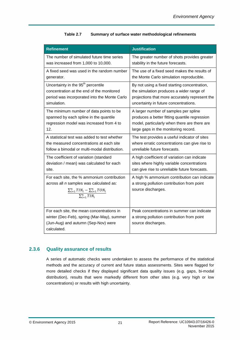
of the results. These refinements are detailed in Table 2.7.
Environment Agency
Report Reference: UC10943.07/16426-0 November 2015
© Environment Agency 2015 21
Table 2.7 Summary of surface water methodological refinements
Refinement Justification
The number of simulated future time series
was increased from 1,000 to 10,000.
The greater number of shots provides greater
stability in the future forecasts.
A fixed seed was used in the random number
generator.
The use of a fixed seed makes the results of
the Monte Carlo simulation reproducible.
Uncertainty in the 95th percentile
concentration at the end of the monitored
period was incorporated into the Monte Carlo
simulation.
By not using a fixed starting concentration,
the simulation produces a wider range of
projections that more accurately represent the
uncertainty in future concentrations.
The minimum number of data points to be
spanned by each spline in the quantile
regression model was increased from 4 to
12.
A larger number of samples per spline
produces a better fitting quantile regression
model, particularly when there are there are
large gaps in the monitoring record.
A statistical test was added to test whether
the measured concentrations at each site
follow a bimodal or multi-modal distribution.
The test provides a useful indicator of sites
where erratic concentrations can give rise to
unreliable future forecasts.
The coefficient of variation (standard
deviation / mean) was calculated for each
site.
A high coefficient of variation can indicate
sites where highly variable concentrations
can give rise to unreliable future forecasts.
For each site, the % ammonium contribution
across all n samples was calculated as:
∑ 𝑇𝐼𝑁𝑖𝑛𝑖=1 − ∑ 𝑇𝑂𝑁𝑖
𝑛𝑖=1
∑ 𝑇𝐼𝑁𝑖𝑛𝑖=1
A high % ammonium contribution can indicate
a strong pollution contribution from point
source discharges.
For each site, the mean concentrations in
winter (Dec-Feb), spring (Mar-May), summer
(Jun-Aug) and autumn (Sep-Nov) were
calculated.
Peak concentrations in summer can indicate
a strong pollution contribution from point
source discharges.
2.3.6 Quality assurance of results
A series of automatic checks were undertaken to assess the performance of the statistical
methods and the accuracy of current and future status assessments. Sites were flagged for
more detailed checks if they displayed significant data quality issues (e.g. gaps, bi-modal
distribution), results that were markedly different from other sites (e.g. very high or low
concentrations) or results with high uncertainty.

Environment Agency
Report Reference: UC10943.07/16426-0 November 2015
© Environment Agency 2015 22
Visual checks of the Weibull estimates, quantile regression trends and future forecasts,
plotted against the raw data, were undertaken by WRc for sites:
with unusually high average or maximum concentrations;
with unusually high or low forecasts of current and future concentrations;
with an unusually high coefficient of variation;
with a statistically significant bimodal or multi-modal distribution;
with large gaps in the monitoring record, or no recent monitoring data;
that had an unusually wide confidence interval around the results;
that failed the current or future status tests despite no samples exceeding the 11.29
threshold;
that passed the current and future status tests but had exceedances of the 11.29
threshold since 2009; and
where there was a large discrepancy between the Weibull and quantile regression
estimates of the current 95th percentile concentration.
Checks focused on sites that met more than one criterion for checking, and those where
highly variable concentrations made it difficult to characterise accurately the historical water
quality trends. In general, the checks confirmed that the statistical methodology had been
applied correctly and that the current and future status assessments were reasonable at the
vast majority of sites. However, they also revealed a small minority of sites where:
a small number of high or low measurements were exerting a high degree of influence
on the results;
strongly fluctuating concentrations meant that historical trends could not be
characterised adequately, with the result that future forecasts were over/under-
estimated or very uncertain; or
large gaps in the monitoring record made the results particularly sensitive to historical
trends or a small number of recent samples.
Monitoring sites were flagged for the Environment Agency’s attention where the results were
judged not to be a reasonable representation of current and future water quality.

Environment Agency
Report Reference: UC10943.07/16426-0 November 2015
© Environment Agency 2015 23
3. Groundwater methodology
3.1 Source datasets
3.1.1 Environment Agency monitoring data
The EA extracted from its WIMS database all water quality data collected at routine
groundwater monitoring sites in England between 1980 and 2015. The determinand codes
extracted were:
0111 (Ammoniacal nitrogen as N);
0116 (Total oxidised nitrogen as N);
0117 (Nitrate as N);
0118 (Nitrite as N); and
9880 (Nitrate as NO3).
Measurements with purpose codes relating to reactive sampling of pollution incidents and
monitoring of waste sites were not provided as they were thought to be unrepresentative of
normal water quality. Table 3.1 shows which purpose codes were contained within the data
provided by the EA.
Table 3.1 Purpose codes included in groundwater dataset
Purpose
Code Purpose Code Description
Included
CA Compliance audit (permit) Yes
CF Compliance formal (permit) No
CI Statutory audit (operator data) Yes
CO Water quality UWWTD monitoring data Yes
CS Water quality operator self-monitoring compliance data Yes
IA IPPC/IPC monitoring (Agency audit – permit) Yes
IF IPPC/IPC monitoring (formal sample) No
II IPPC/IPC monitoring (Agency investigation) Yes
IO IPPC/IPC monitoring (operator self-monitoring data) Yes

Environment Agency
Report Reference: UC10943.07/16426-0 November 2015
© Environment Agency 2015 24
Purpose
Code Purpose Code Description
Included
IT Instrument trial No
MI Statutory failures (follow ups at designated points) No
MN Monitoring (national Agency policy) Yes
MP Environmental monitoring (GQA & RE only) Yes
MS Environmental monitoring statutory (EU directives) Yes
MU Monitoring (UK govt policy – not GQA or RE) Yes
PF Planned formal non-statutory (permit/env mon) No
PI Planned investigation (operational monitoring) No
PN Planned investigation (national Agency policy) Yes
SI Statutory failures (follow ups at non-designated points) No
UF Unplanned reactive monitoring formal (pollution incidents) No
UI Unplanned reactive monitoring (pollution incidents) No
WA Waste monitoring (Agency audit – permit) No
WF Waste monitoring (formal sample) No
WI Waste monitoring (Agency investigation) No
WO Waste monitoring (operator self-monitoring data) No
XO External organisation monitoring Yes
ZZ Unspecified at time of WIMS load No
The raw dataset contained 6663 unique monitoring points and 310,958 unique samples.
3.1.2 Water company monitoring data
Defra invited water companies to provide surface water quality data collected as part of their
routine monitoring programmes. Six companies provided valid data (including co-ordinates)
for a total of 259,004 samples from 706 unique surface water monitoring sites. Table 3.2
provides a summary for each water company.
Environment Agency
Report Reference: UC10943.07/16426-0 November 2015
© Environment Agency 2015 25
Table 3.2 Summary of water company surface water dataset
Water Company Determinands recorded Sites Samples Date span
Affinity Water Nitrate as N,
Nitrite as N,
Nitrogen, Total Oxidised as N
150 13,023 Aug 1999 –
June 2014
Bristol Water Nitrate as NO3 17 14,369 Feb 1995 –
March 2015
Sutton and East
Surrey
Nitrate as NO3 16 1,050 Nov 1992 –
Dec 2014
United Utilities Ammoniacal Nitrogen as N
Nitrate as N
Nitrite as N
Nitrogen, Total Oxidised as N
112 16,087 Feb 1980 –
April 2015
Wessex Water Nitrate as N 333 187,149 Dec 1979 –
April 2015
Yorkshire Water Nitrate as N 78 27,326 Jan 1980 –
April 2015
Totals 706 259,004
3.2 Data processing
3.2.1 Monitoring sites
Since the EA monitoring network includes some sites with the same ID in different regions, a
unique Site ID was created for each EA monitoring site by combining the Site ID and EA
Region fields. For water company data, a unique Site ID was created by combining the Site ID
and abbreviated water company name.
Data supplied to the EA by external organisations (Purpose Code = XO) was included in the
WIMS dataset, creating a risk that some water company monitoring data may have been
supplied by both the EA and the water company. The EA and water company datasets were
therefore compared to identify duplicate monitoring points. Site IDs were not always
consistent between the two datasets, so sites were matched on their co-ordinates. A total of
460 sites with matching co-ordinates were found in both datasets. We attempted to confirm
whether or not these pairs of sites were truly the same monitoring point but this was not
possible because:
clusters of boreholes frequently share the same co-ordinates; and

Environment Agency
Report Reference: UC10943.07/16426-0 November 2015
© Environment Agency 2015 26
some pairs of sites had the same site name in both datasets, but many pairs had subtle
differences (i.e. leading zeros or letters) or completely different names, which
prevented them being matched.
Rather than risk merging data from different monitoring points, the pairs of sites were retained
as two separate monitoring points and analysed separately. By adopting this approach, it is
likely that some sites and samples have been duplicated in the analysis, but because they
have identical locations this does not overstate the degree of evidence for or against
designation.
The co-ordinates of each monitoring site were checked for missing or inconsistent eastings
and northings, but no issues were found for the EA data. Some water company sites were
missing co-ordinates but these were retained in case valid grid references could be provided
at a later date.
The following meta-data were tabulated for each monitoring site:
unique Site ID;
site name;
co-ordinates (eastings and northings);
site operator (Environment Agency or Water Company);
EA sampling point type (where applicable); and
EA region (where applicable).
As far as possible, the EA and water company datasets were filtered to exclude monitoring
sites that sampled water after it had been treated to remove nitrate (and so is not
representative of raw water quality) or sampled water that had been blended from multiple
sources. To achieve this, the EA dataset was filtered according to the sampling point types
listed in Table 3.3. The same filter was applied to the Affinity Water and Sutton and East
Surrey Water datasets, which had also been extracted from the EA’s WIMS database. For the
remaining four water companies, all surface water monitoring sites were assumed to sample
untreated and unblended river water.

Environment Agency
Report Reference: UC10943.07/16426-0 November 2015
© Environment Agency 2015 27
Table 3.3 Sampling point types included in groundwater analysis
Sampling Point Type Code Sampling Point Description Included
BA Groundwater – borehole Yes
BB Groundwater – spring Yes
BC Groundwater – wells & adits Yes
BD Groundwater – pit Yes
BE Groundwater – composite Yes
BH Groundwater – landfill site No
BL Groundwater – external to landfill site No
BZ Groundwater – unspecified Yes
3.2.2 Samples
For the EA WIMS dataset, a Unique Sample ID was created for each sample by combining
the UniqueSiteID, Sample Reference Number and Date (yyyy/mm/dd) fields. For the water
company dataset a Unique Sample ID was created for each sample by combining the
UniqueSiteID, Date and Time fields (or, for United Utilities, the UniqueSiteID and Date fields
only as no Time field was available).
Samples collected before 1st January 1980 were excluded because they were not regarded as
indicative of recent nitrate trends. Samples collected after 31st December 2014 were also
excluded because a full calendar year of monitoring data was not available for 2015 and,
where water quality fluctuates seasonally, the use of incomplete years could cause current
nitrate concentration to be over- or under-estimated.
The data were screened to identify how many samples were taken from each site on each
day. In most cases, a single water sample was taken from a given site on a given day, but
multiple samples were sometimes taken. Autosamplers are not usually deployed at
groundwater monitoring sites, but multiple samples may be taken from different depths within
a borehole, from a set of adjacent boreholes (that share a Site ID), or for some other
investigative purpose. The presence of multiple samples means that any analysis of nitrate
concentrations is weighted towards days when more samples are taken so we adopted the
following rule to prevent this occurring.
Where two or more samples had been taken from the same site on the same day, the
sample with the highest TIN reading was retained and the other samples excluded. If
the two TIN readings were identical then the sample with the highest TON was retained
and if the TIN and TON readings were identical the sample with the highest sample
number was retained.

Environment Agency
Report Reference: UC10943.07/16426-0 November 2015
© Environment Agency 2015 28
In the case of United Utilities, the time of each sample was not recorded and so an average
concentration was calculated for each determinand on each day, and these daily average
values were used to calculate TIN and TON concentrations as described in Section 3.2.3
below.
If neither TON nor nitrate was measured (i.e. the sample only had measurements for nitrite
and/or ammonium) then the sample was excluded.
3.2.3 Determinands
Most water samples were measured for multiple determinands. These determinand results
were combined to calculate the concentration of total inorganic nitrogen (TIN) and total
oxidised nitrogen (TON) in each sample, as described below.
To make all determinands comparable, measurements recorded in mg/l as NO3 were
converted to mg/l as N by multiplying by 0.2258. Thus, 50 mg NO3/l corresponds to 11.29 mg
N/l.
Zero readings were removed. These can arise for a variety of reasons, but it cannot be
assumed that they represent readings below the Limit of Detection (LOD). Negative readings
were also removed as these are clearly erroneous.
“Less than” values were treated using the standard EA approach of dividing the recorded
concentration by two. “Greater than” values were not very prevalent in the data and were not
adjusted (i.e. the concentration measurement was used as reported).
Total Inorganic Nitrogen (TIN) was calculated by the following rules, listed in order of
declining preference:
= TON + ammonium;
= nitrate + nitrite + ammonium;
= TON;
= nitrate + nitrite;
= nitrate + ammonium;
= nitrate.
Total Oxidised Nitrogen (TON) was calculated by the following rules, listed in order of
declining preference:
= TON;
= nitrate + nitrite;
Environment Agency
Report Reference: UC10943.07/16426-0 November 2015
© Environment Agency 2015 29
= nitrate.
TIN and TON were not calculated if TON and nitrate were both missing, but were calculated if
nitrite and/or ammonium were missing because these determinands typically represent only a
small proportion of the nitrogen in the water sample.
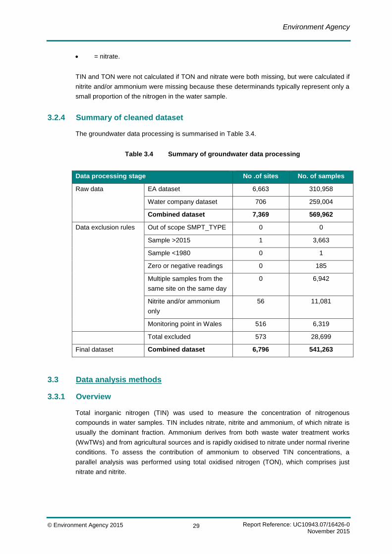
3.2.4 Summary of cleaned dataset
The groundwater data processing is summarised in Table 3.4.
Table 3.4 Summary of groundwater data processing
Data processing stage No .of sites No. of samples
Raw data EA dataset 6,663 310,958
Water company dataset 706 259,004
Combined dataset 7,369 569,962
Data exclusion rules Out of scope SMPT_TYPE 0 0
Sample >2015 1 3,663
Sample <1980 0 1
Zero or negative readings 0 185
Multiple samples from the
same site on the same day
0 6,942
Nitrite and/or ammonium
only
56 11,081
Monitoring point in Wales 516 6,319
Total excluded 573 28,699
Final dataset Combined dataset 6,796 541,263
3.3 Data analysis methods
3.3.1 Overview
Total inorganic nitrogen (TIN) was used to measure the concentration of nitrogenous
compounds in water samples. TIN includes nitrate, nitrite and ammonium, of which nitrate is
usually the dominant fraction. Ammonium derives from both waste water treatment works
(WwTWs) and from agricultural sources and is rapidly oxidised to nitrate under normal riverine
conditions. To assess the contribution of ammonium to observed TIN concentrations, a
parallel analysis was performed using total oxidised nitrogen (TON), which comprises just
nitrate and nitrite.

Environment Agency
Report Reference: UC10943.07/16426-0 November 2015
© Environment Agency 2015 30
Each groundwater monitoring site with sufficient data was analysed to determine whether or
not:
the 95th percentile TIN concentration currently exceeds 50 mg NO3/l; or,
the 95th percentile TIN concentration is likely to exceed 50 mg NO3/l in the future,
assuming no preventative action is taken.
Following the 2013 Review methodology, a site was deemed to have failed the statistical test
if the current or future 95th percentile nitrate concentration exceeded 50 mg NO3/l with at least
95% confidence. In practice this meant testing whether the lower 90% confidence limit on the
95th percentile exceeded 50 mg NO3/l. This approach is slightly less stringent than that for
surface waters (which uses the best estimate of the 95th percentile instead of the lower
confidence limit) and amounts to setting the evidence bar slightly higher to reduce the risk of
falsely designating NVZs due to high sampling errors. In other words, this approach is a way
of taking account of the uncertainty that arises when limited monitoring data is available for
analysis.
The year 2027 was chosen as the time horizon for the future assessment because it (i) is
consistent with the approach used in the 2013 NVZ Review, (ii) allows a sufficient period of
time for pollution mitigation measures to take effect, and (iii) ties in with the Water Framework
Directive river basin planning cycle.
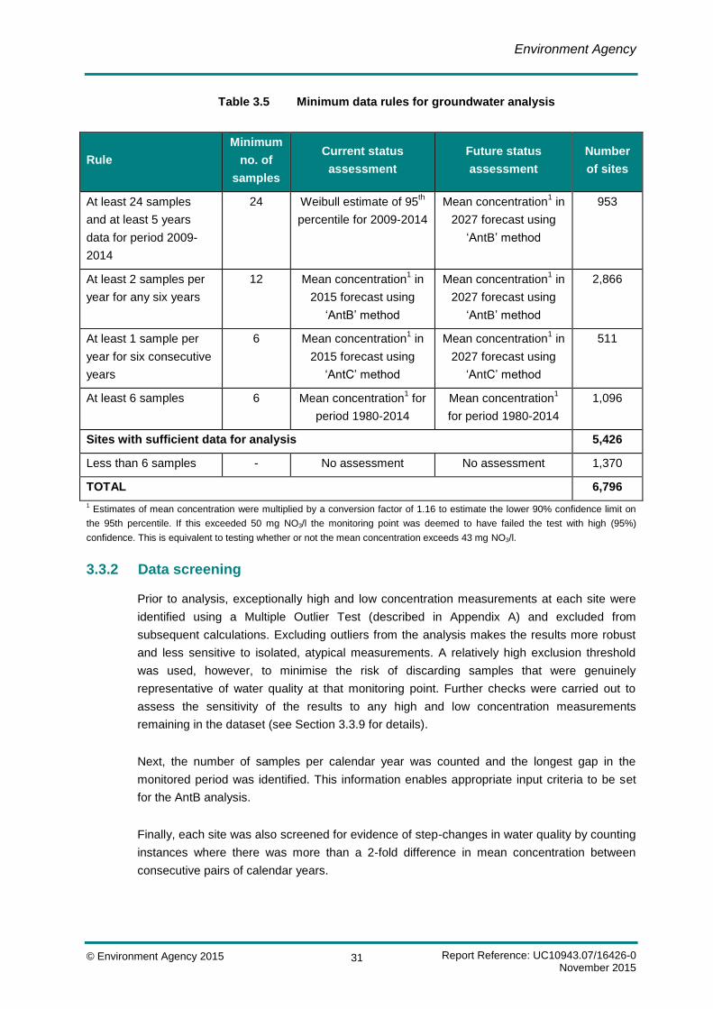
The statistical methods used to assess current and future status at each monitoring point
depended upon the amount of data available, as set out in Table 3.5. As in the 2013 NVZ
Review, most sites had insufficient data to robustly estimate the 95th percentile concentration.
For these sites, the mean concentration was estimated instead and a conversion factor of
1.16 was applied to convert the mean concentration into an estimate of the lower 90%
confidence limit on the 95th percentile (see Section 3.3.7 for details). This is equivalent to
testing whether or not the mean TIN concentration exceeds 43 mg NO3/l.
The assessment of current status used data from the last six calendar years (i.e. 2009-2014)
to estimate the 95th percentile concentration or, where less data were available, a statistical
extrapolation of the historical (1980-2014) time series was used to predict the mean
concentration in mid-2015. The assessment of future status used the same statistical
extrapolation methods to predict the mean concentration in mid-2027. To ensure that the
results of the analysis were based on sound monitoring evidence, sites were not assessed if
they had fewer than six water quality samples in total.
All statistical analyses were conducted using R v. 3.2.0 (R Core Team 2015).
Environment Agency
Report Reference: UC10943.07/16426-0 November 2015
© Environment Agency 2015 31
Table 3.5 Minimum data rules for groundwater analysis
Rule
Minimum
no. of
samples
Current status
assessment
Future status
assessment
Number
of sites
At least 24 samples
and at least 5 years
data for period 2009-
2014
24 Weibull estimate of 95th
percentile for 2009-2014
Mean concentration1 in
2027 forecast using
‘AntB’ method
953
At least 2 samples per
year for any six years
12 Mean concentration1 in
2015 forecast using
‘AntB’ method
Mean concentration1 in
2027 forecast using
‘AntB’ method
2,866
At least 1 sample per
year for six consecutive
years
6 Mean concentration1 in
2015 forecast using
‘AntC’ method
Mean concentration1 in
2027 forecast using
‘AntC’ method
511
At least 6 samples 6 Mean concentration1 for
period 1980-2014
Mean concentration1
for period 1980-2014
1,096
Sites with sufficient data for analysis 5,426
Less than 6 samples - No assessment No assessment 1,370
TOTAL 6,796
1 Estimates of mean concentration were multiplied by a conversion factor of 1.16 to estimate the lower 90% confidence limit on
the 95th percentile. If this exceeded 50 mg NO3/l the monitoring point was deemed to have failed the test with high (95%)
confidence. This is equivalent to testing whether or not the mean concentration exceeds 43 mg NO3/l.
3.3.2 Data screening
Prior to analysis, exceptionally high and low concentration measurements at each site were
identified using a Multiple Outlier Test (described in Appendix A) and excluded from
subsequent calculations. Excluding outliers from the analysis makes the results more robust
and less sensitive to isolated, atypical measurements. A relatively high exclusion threshold
was used, however, to minimise the risk of discarding samples that were genuinely
representative of water quality at that monitoring point. Further checks were carried out to
assess the sensitivity of the results to any high and low concentration measurements
remaining in the dataset (see Section 3.3.9 for details).
Next, the number of samples per calendar year was counted and the longest gap in the
monitored period was identified. This information enables appropriate input criteria to be set
for the AntB analysis.
Finally, each site was also screened for evidence of step-changes in water quality by counting
instances where there was more than a 2-fold difference in mean concentration between
consecutive pairs of calendar years.

Environment Agency
Report Reference: UC10943.07/16426-0 November 2015
© Environment Agency 2015 32
3.3.3 Weibull method
The Weibull method was used to estimate the current 95th percentile concentration at
monitoring points that had at least 24 water quality samples and five years with data between
2009 and 2014.
The Weibull protocol is a robust technique because it doesn’t make any prior assumption
about the underlying distribution of the data (i.e. it doesn’t require the data to follow a normal
or log-normal distribution). It is also relatively insensitive to outliers and provides an
assessment of conditions over a six year period, which averages out year to year variation
and makes the results insensitive to random, short-term fluctuations in water quality.
The Weibull method uses the rth ranked value within the observation dataset to provide an
estimate of the 95th percentile, where r = 0.95(n + 1) and n is the number of samples. When r
is not an integer, r is rounded down and up to the nearest whole number, and the
corresponding concentration values for these ranks are interpolated to estimate the 95th
percentile. Conservative 90% confidence intervals were calculated using binomial distribution
theory, as described in the EA Codes of Practice for Data Handling (Ellis et al., 1993). If the
lower 90% confidence limit exceeded 50 mg NO3/l, the monitoring point was deemed to have
failed the test.
3.3.4 AntB method
The AntB tool was used to forecast current (mid-2015) and future (mid-2027) mean nitrate
concentrations at monitoring points that had at least two samples per year for any six years
between 1980 and 2014.
AntB is a simplified version of ANTEATER, a statistical forecasting tool for groundwater nitrate
that was developed for the Environment Agency by WRc in the late 1990s. One limitation of
ANTEATER is that a substantial amount of monitoring data is needed for it to work
satisfactorily. A simplified version of ANTEATER called AntB was therefore developed in
2005. This applies a broadly similar methodology to that used by ANTEATER, but is aimed at
datasets that are not sufficiently extensive for a full ANTEATER analysis to be possible.
The operations undertaken by AntB fall into two main parts:
1. trend analysis – AntB characterises historical changes in mean nitrate concentration;
and
2. forecasting – AntB uses Monte Carlo simulation to extrapolate the historical trend and
forecast future nitrate concentration.
The statistical methodology used in AntB is discussed below under these headings.
Environment Agency
Report Reference: UC10943.07/16426-0 November 2015
© Environment Agency 2015 33
Trend analysis
A multiple regression model was fitted to the data to characterise historical variation in the
mean concentration at each monitoring site. The model consisted of two main elements: a
linear spline component, which represents inter-annual changes in mean nitrate concentration
as a series of k straight lines connected by k-1 ‘hinge points’, and a seasonal sinusoidal
component, which represents within-year changes in mean nitrate concentration.
Inter-annual trends
Hinge points were constrained to occur at the end of calendar years to avoid picking up
seasonal effects. The following rules were used to strike an appropriate balance between
having too many splines (whose estimation would then be excessively vulnerable to high-
influence points in the data) and too few splines (which might be unable to reflect genuine
historical zigzags).
So that future changes in nitrate concentration could be simulated using a fixed time
step, the splines must be of equal length (i.e. span the same number of calendar years.
The exception was where the number of years per spline is not an exact multiple of the
total number of years in the data set. In this situation any remainder years are included
in the final spline; for example, 4 splines over 18 years would span 4, 4, 4, and 6 years.
To prevent over-fitting, the maximum allowed number of splines was 10.
To make the trend results more robust to high-influence data points, the average
number of data points per linear spline must be at least 6. This minimum must be met
not just on average, but also for the two end splines.
The splines must be apportioned over the full time period of the monitoring data,
(including years with no data) and long enough to span any gaps in the monitoring
record. For instance, if the biggest gap in the data extends for Y calendar years, the
number of years per spline must be at least Y + 1.
Seasonal trends
AntB represents seasonality using a simple sinusoidal function: Sin(2X) + Cos(2X), where
X is the decimal fraction of the year (ranging from 0 to 1). If BS and BC are the resulting slope
estimates, the amplitude and phase of the seasonal term are then estimated by:
Amplitude = (BS2 + BC
2), and
Phase = ArcTan(-BC/BS) + c,
where c is an adjustment factor set to 0, +1 or -1 as appropriate to make Cos(Phase) have
the same sign as BS.

Environment Agency
Report Reference: UC10943.07/16426-0 November 2015
© Environment Agency 2015 34
Consideration was given to extending the analysis to allow the amplitude to vary from year to
year, but groundwater data is often too erratic or sparse in individual years for this to work
reliably, and so AntB uses a constant amplitude and phase.
Trend analysis
The relationship between nitrate concentration and time was calibrated using multiple
regression, with one appropriately defined dummy variable per spline and two additional
predictor variables to represent seasonality. The linear spline and seasonal terms were
forcibly included, and carried through into the forecasting phase, regardless of whether or not
they were statistically significant. The justification for including them in the latter case is that
they are still the best estimates of the historical trends – and if they are not statistically
significant the sizes of the effects are likely to be relatively slight.
Forecasting
Monte Carlo simulation was used to extrapolate the historical trend and forecast future water
quality at each site. The simulation assumes that the 35 years of historical data provides the
best (unbiased) evidence as to the likely future direction of water quality and is constructed by
selecting slopes at random from a defined population of spline slopes.
Suppose the historical multiple regression model has m splines. In general, some of these
spline slopes will have been estimated less precisely than others – as reflected by their
standard errors (SE). The simulation allows for this by defining the weight for spline slope j to
be proportional to 1/SE(j) and, using these weights, calculating the weighted mean (AvB) and
weighted standard deviation (SDB) of the m spline slopes. If the model contained a just single
spline, then SDB was estimated as double the standard error of the spline slope coefficient.
The other inputs to the forecasting are:
the final spline slope;
the lag-1 autocorrelation of the spline slopes, R1, which defaults to 0 if there are fewer
than 4 splines;
the number of years per spline (except possibly for the last spline); and
the predicted mean concentration at the end of the monitored period (τ) and its
standard error (τSE).
Taking as its starting point a mean concentration drawn from the Normal distribution N(τ, τSE)
and the final spline slope, the simulation generates a projection of how the mean nitrate
concentration might change in the future, starting from the year immediately following the end
of the monitoring record.

Environment Agency
Report Reference: UC10943.07/16426-0 November 2015
© Environment Agency 2015 35
The future projection is constructed by selecting a series of spline slopes at random from the
Normal distribution N(AvB, SDB), and loosely associating each with the preceding slope to an
extent governed by the autocorrelation coefficient R1. Specifically, the slope for time step i+1
is generated from the previous time step’s slope (Bi) and the random slope (Brand) as follows:
Bi+1 = (1 – R1) AvB + R1 Bi + (1 – R12) ( Brand – AvB).
Taking the spline length as the time step, the process is continued until the required
forecasting horizon is reached. Starting from mid-2011, for example, if the spline length was 4
years, a series of four slopes would be generated to predict the mean concentration in mid-
2027.
The whole process was repeated 10,000 times to generate a range of possible ‘futures’. A
variety of summary statistics were harvested from each of the 10,000 simulated time series,
including the median, which represents the best estimate of the mean concentration in mid-
2015 and mid-2027. The uncertainty in this estimate was quantified by ranking the 10,000
forecasts for that year and determining the 10th, 25
th, 75
th and 90
th percentile values.
Finally, a conversion factor was applied to convert the mean concentration to an estimate of
the 95th percentile concentration (see Section 3.3.7).
Figure 3.1 shows an example of a fitted AntB regression model and the forecasts generated
from it. The horizontal green dashed line at 11.29 mg N/l (equivalent to 50 mg NO3/l) indicates
the threshold value for the 95th percentile concentration and the horizontal blue dashed line at
9.71 mg N/l indicates the corresponding threshold value for the mean concentration
(equivalent to 43 mg NO3/l).
The solid blue wavy line indicates historical fluctuations in the mean concentration. Beyond
the end of the monitoring record in 2007:
the blue line indicates the mean concentration forecast by Monte Carlo simulation;
the blue shaded band indicates the 50% confidence interval around the mean estimate;
and
the wider, light blue shaded band indicates the 90% confidence interval around the
mean estimate.
In this example, the mean concentration is forecast to be 8.2 mg N/l in mid-2015 (the first
vertical dashed line) with a 90% confidence interval of 6.5-9.9 mg N/l, and 8.6 mg N/l in mid-
2027 (the second vertical dashed line) with a 90% confidence interval of 4.1-13.1 mg N/l.

Environment Agency
Report Reference: UC10943.07/16426-0 November 2015
© Environment Agency 2015 36
Figure 3.1 Historical trend and future forecast of mean nitrate concentration using
AntB, and comparison to the 9.71 mg N/l (43 mg NO3/l) standard (horizontal blue
dashed line)
3.3.5 AntC method
The AntC tool was used to forecast current (mid-2015) and future (mid-2027) mean nitrate
concentration at monitoring points that had at least one sample per year for six consecutive
years at some point between 1980 and 2014. If there was more than one suitable period
within the sample data for a selected site, the most recent period was analysed.
AntC is a simplified version of AntB, which is used when there are insufficient samples to
characterise seasonal variation. AntC uses a simplified version of AntB’s spline model to

Environment Agency
Report Reference: UC10943.07/16426-0 November 2015
© Environment Agency 2015 37
characterise historical trends in annual mean concentrations and, like AntB, uses Monte Carlo
simulation to extrapolate the historical trend and forecast future nitrate concentrations.
The operations undertaken by AntC fall into two main parts:
1. trend analysis – AntC characterises historical changes in mean nitrate concentration;
and
2. forecasting – AntC uses Monte Carlo simulation to extrapolate the historical trend and
forecast future nitrate concentration.
The statistical methodology used in AntC is discussed below under these headings.
Trend analysis
First, annual mean concentrations (Y1, Y2, etc. up to Yk,) are calculated for the k consecutive
years of data (i.e. replicate samples taken in the same year are averaged together). The k-1
successive differences between these annual means are then calculated as:
Di = Yi+1 – Yi, i running from 1 to k-1.
and used to quantify the direction and rate of change in water quality over time.
Forecasting
The inputs to the forecasting are:
the average (AvD) and standard deviation (SDD) of the k-1 successive differences
between the annual means; and
the lag-1 autocorrelation of the successive differences, R1.
Given the generally precarious nature of the data set being analysed, a precautionary
adjustment to the SDD was made by setting it to the upper 90% confidence limit. Thus:
SDD = SDD√[(k-2)/ChiSqd],
where ChiSqd is the 10% point of the chi-squared distribution with k-2 degrees of freedom.
For example, with 10 years of data, N = 10, and so the factor by which SDD is scaled up is
√[8/3.49] = 1.51.
Taking as its starting point the mean concentration in the last of the k consecutive years, the
simulation generates a projection of how the mean nitrate concentration might change in the
future. The future projection is constructed by selecting a series of annual difference values at

Environment Agency
Report Reference: UC10943.07/16426-0 November 2015
© Environment Agency 2015 38
random from the Normal distribution N(AvD, SDD), and loosely associating each with the
preceding difference to an extent governed by the autocorrelation coefficient R1. Specifically,
the difference for year i+1 is generated from the previous year’s difference (Bi) and the
random difference (Brand) as follows:
Bi+1 = (1 – R1) AvD + R1 Bi + (1 – R12) ( Brand – AvD).
The process is continued on an annual time step, cumulatively adding the differences
together, until the required forecasting horizon is reached. If the last of the consecutive years
was 2014, for example, a series of 13 annual differences would be generated to predict the
mean concentration in mid-2027.
The whole process was repeated 10,000 times to generate a range of possible ‘futures’. A
variety of summary statistics were harvested from each of the 10,000 simulated time series,
including the median, which represents the best estimate of the mean concentration in mid-
2015 and mid-2027. The uncertainty in this estimate was quantified by ranking the 10,000
forecasts for that year and determining the 10th, 25
th, 75
th and 90
th percentile values.
Finally, a conversion factor was applied to convert the mean concentration to an estimate of
the 95th percentile concentration (see Section 3.3.7).
Figure 3.2 shows an example of a fitted AntC model and the forecasts generated from it. The
horizontal green dashed line at 11.29 mg N/l (equivalent to 50 mg NO3/l) indicates the
threshold value for the 95th percentile concentration and the horizontal blue dashed line at
9.71 mg N/l (equivalent to 43 mg NO3/l) indicates the corresponding threshold value for the
mean concentration.
The observed annual mean concentrations are shown by short horizontal blue lines. Beyond
the end of the monitoring record in 2014:
the solid blue line indicates the mean concentration forecast by Monte Carlo simulation;
the blue shaded band indicates the 50% confidence interval around the mean estimate;
and
the wider, light blue shaded band indicates the 90% confidence interval around the
mean estimate.
In this example, the mean concentration is forecast to be 7.2 mg N/l in mid-2015 (the first
vertical dashed line) with a 90% confidence interval of 6.3-8.1 mg N/l, and 8.3 mg N/l in mid-
2027 (the second vertical dashed line) with a 90% confidence interval of 0.0-16.8 mg N/l.

Environment Agency
Report Reference: UC10943.07/16426-0 November 2015
© Environment Agency 2015 39
Figure 3.2 Historical trend and future forecast of mean nitrate concentration using
AntC, and comparison to the 9.71 mg N/l (43 mg NO3/l) standard (horizontal blue
dashed line)
3.3.6 Mean Concentration method
At sites where there were insufficient data to apply the Weibull, AntB or AntC methods, the
mean concentration of all the samples (1980-2014) was calculated and taken as an estimate
of the mean concentration in mid-2015 and mid-2027. The standard deviation of historical
data was used to calculate the 50% and 90% confidence intervals around the mean estimate.
Finally, a conversion factor was applied to convert the mean concentration to an estimate of
the 95th percentile concentration (see Section 3.3.7).
Figure 3.3 shows an example of a monitoring point where the mean concentration of the
historical dataset is used to assess current and future water quality. The horizontal green

Environment Agency
Report Reference: UC10943.07/16426-0 November 2015
© Environment Agency 2015 40
dashed line at 11.29 mg N/l (equivalent to 50 mg NO3/l) indicates the threshold value for the
95th percentile concentration and the horizontal blue dashed line at 9.71 mg N/l (equivalent to
43 mg NO3/l) indicates the corresponding threshold value for the mean concentration.
The observed historical mean concentration is shown by the solid blue horizontal line. Beyond
the end of the monitoring record in 2011:
the solid blue line indicates the future forecast of mean concentration;
the blue shaded band indicates the 50% confidence interval around the mean estimate;
and
the wider, light blue shaded band indicates the 90% confidence interval around the
mean estimate.
In this example, the mean concentration in mid-2015 (the first vertical dashed line) and mid-
2027 (the second vertical dashed line) is forecast to be 13.0 mg N/l with a 90% confidence
interval of 10.8-15.2 mg N/l.

Environment Agency
Report Reference: UC10943.07/16426-0 November 2015
© Environment Agency 2015 41
Figure 3.3 Historical trend and future forecast of mean nitrate concentration using
the ‘Mean Concentration’ method, and comparison to the 9.71 mg N/l (43 mg NO3/l)
standard (horizontal blue dashed line)
3.3.7 Conversion factor
The 95th percentile is the primary statistic used to measure nitrate concentrations in surface
waters and groundwater. Unlike surface waters, however, most groundwater monitoring sites
lack sufficient data to robustly estimate the 95th percentile concentration. Since the kriging
process (Section 3.4) requires the same summary statistic to be used for all monitoring points,
a conversion factor was used to make estimates of mean and 95th percentile concentrations
comparable.
During the 2008 Review the mean concentration was estimated for all monitoring points and
the compliance threshold of 50 mg NO3/l (or 11.29 mg N/l) was adjusted to take into account
the fact that the mean is always lower than the 95th percentile. Based on the sample

Environment Agency
Report Reference: UC10943.07/16426-0 November 2015
© Environment Agency 2015 42
distribution for all groundwater samples, a threshold of 45 mg NO3/l (or 10.16 mg N/l) was
chosen (Defra 2008). The choice of 45 mg NO3/l was informed by an analysis which showed
that the mean concentration was on average 5 mg NO3/l lower than the lower 90% confidence
limit on the 95th percentile for monitoring points with large numbers of samples. This provided
a comparable level of protection for groundwater to that achieved by the statistical test for
surface waters.
During the 2013 Review, a re-analysis of the “45 mg/l rule” using up-to-date monitoring data
recommended that a conversion factor of 50/43 (or 1.16) would be appropriate. However, the
Methodology Review Group opted to use a conversion factor of 50/45 (or 1.11) for
consistency with the 2008 methodology. Sensitivity analysis indicated that the proportion of
monitoring points failing the test was similar using 1.11 or 1.16. For consistency with the
surface water methodology, the Methodology Review Group took a decision to adopt the 95th
percentile as the primary statistic and to apply a conversion factor of 1.11 to the observed
mean concentrations, so that all results could be compared to a threshold concentration of
50 mg NO3/l.
For the 2017 Review, Defra opted to accept the recommendation of the 2013 Review and
adopt a conversion factor of 1.16. The central estimate of the mean concentration was
therefore multiplied by 1.16 to convert it into an estimate of the lower 90% confidence limit on
the 95th percentile. If this exceeded 50 mg NO3/l the monitoring point was deemed to have
failed the test with high (95%) confidence. This is equivalent to testing whether or not the
mean concentration exceeds 43 mg NO3/l (or 9.71 mg N/l).
3.3.8 Comparison with 2013 Review
Whilst the statistical methodology followed that used for the 2013 NVZ Review as closely as
possible, a small number of refinements were made to improve the accuracy and repeatability
of the results. These refinements are detailed in Table 3.6.
Table 3.6 Summary of groundwater methodological refinements
Refinement Justification
The number of simulated future time series
was increased from 1,000 to 10,000.
The greater number of shots provides greater
stability in the future forecasts.
A fixed seed was used in the random number
generator.
The use of a fixed seed makes the results of
the Monte Carlo simulation reproducible.
Uncertainty in the mean concentration at the
end of the monitored period was incorporated
into the AntB Monte Carlo simulation.
By not using a fixed starting concentration,
the simulation produces a wider range of
projections that more accurately represent the
uncertainty in future concentrations.

Environment Agency
Report Reference: UC10943.07/16426-0 November 2015
© Environment Agency 2015 43
Refinement Justification
A statistical test was added to test whether
the measured concentrations at each site
follow a bimodal or multi-modal distribution.
The test provides a useful indicator of sites
where erratic concentrations can give rise to
unreliable future forecasts.
The coefficient of variation (standard
deviation / mean) was calculated for each
site.
A high coefficient of variation can indicate
sites where highly variable concentrations
can give rise to unreliable future forecasts.
For each site, the % ammonium contribution
across all n samples was calculated as:
∑ 𝑇𝐼𝑁𝑖𝑛𝑖=1 − ∑ 𝑇𝑂𝑁𝑖
𝑛𝑖=1
∑ 𝑇𝐼𝑁𝑖𝑛𝑖=1
A high % ammonium contribution can indicate
a strong pollution contribution from point
source discharges.
For each site, the mean concentrations in
winter (Dec-Feb), spring (Mar-May), summer
(Jun-Aug) and autumn (Sep-Nov) were
calculated.
Peak concentrations in summer can indicate
a strong pollution contribution from point
source discharges.
A time series plot was produced for each
monitoring site, showing the historical data,
fitted trend, and future forecasts.
The plots allow close visual inspection of the
results to verify the assessments of current
and future status.
For AntC, consecutive years are identified
started from the most recent year of
monitoring
In cases where two or more runs of
consecutive years are available, the most
recent data is used, which should provide a
more reliable indicator of current and future
water quality.
To use the Weibull method, there must be at
least one sample in five of the last six years
(2009-14).
This rule brings the groundwater method into
line with the surface water method and
ensure that percentile estimates are based
on data from a small number of potentially
unrepresentative years.
Use of the AntC2 tool for assessing the
status of data-poor groundwater sites was
abandoned in preference of the ‘Mean
Concentration’ method.
Only 15 sites were analysed by AntC2 in the
2013 Review, and only 28 sites meet the
criteria for AntC2 in the 2017 Review. The
predictions from AntC2 typically have a high
degree of uncertainty, and provide little
additional information over the simpler Mean
Concentration method.
The data screening checks used by AntB
were applied to all sites, not just those
analysed using AntB.
The screening checks provide a more
comprehensive data quality check for every
site.

Environment Agency
Report Reference: UC10943.07/16426-0 November 2015
© Environment Agency 2015 44
Refinement Justification
A conversion factor of 50/43 (~1.16) was
applied to estimates of mean concentration to
produce an estimate of the lower 90%
confidence limit on the 95th percentile.
A conversion factor of 50/43 was
recommended at time of the previous NVZ
Review, based upon an analysis of
monitoring data that showed the mean
concentration to be, on average, 7 mg NO3/l
lower than the lower 90% confidence limit on
the 95th percentile.
3.3.9 Quality assurance of results
A series of automatic checks were undertaken to assess the performance of the statistical
methods and the accuracy of current and future status assessments. Sites were flagged for
more detailed manual checks if they displayed significant data quality issues (e.g. gaps, bi-
modal distribution), results that were markedly different from other sites (e.g. very high or low
concentrations) or results with high uncertainty.
In addition, the effect of the refinements described in Section 3.3.8 was assessed by
comparing the results of the original (2013 Review) and revised (2017 Review) methods.
Sites where current estimates showed discrepancies of more than 10% and 1 mg N/l were
reviewed to understand why the results were sensitive to small changes in methodology.
Visual checks of the Weibull estimates, quantile regression trend analysis and future
forecasts, plotted against the raw data, were undertaken by WRc for sites:
with unusually high average or maximum concentrations;
with unusually high or low forecasts of current and future concentrations;
with an unusually high coefficient of variation;
with a statistically significant bimodal or multi-modal distribution;
with large gaps in the monitoring record, or no recent monitoring data;
that had an unusually wide confidence interval around the results;
that failed the current or future status tests despite no samples exceeding the 11.29
threshold;

Environment Agency
Report Reference: UC10943.07/16426-0 November 2015
© Environment Agency 2015 45
that passed the current and future status tests but had exceedances of the 11.29
threshold since 2009;
where there was a large discrepancy between the results generated by the original
(2013 Review) and revised (2017 Review) methods.
Checks focused on sites that met more than one criterion for checking, and those where
highly variable concentrations made it difficult to characterise accurately the historical water
quality trends. In general, the checks confirmed that the statistical methodology had been
applied correctly and that the current and future status assessments were reasonable at the
vast majority of sites. However, they also revealed a small minority of sites where:
a small number of high or low measurements were exerting a high degree of influence
on the results;
strongly fluctuating concentrations meant that historical trends could not be
characterised adequately, with the result that future forecasts were over/under-
estimated or very uncertain; or
large gaps in the monitoring record made the results particularly sensitive to historical
trends or a small number of recent samples.
Monitoring sites were flagged for the Environment Agency’s attention where the results were
judged not to be a reasonable representation of current and future water quality.
3.4 Kriging
3.4.1 Introduction
Monitoring data from groundwater monitoring points only gave groundwater nitrate
concentrations at specific discrete locations within aquifers (the exact area of land
represented by a monitoring point will depend on the volume and depth of the abstraction and
geology). In order to estimate nitrate concentrations across the country and use the
methodology at a 1 km2 resolution, a statistical interpolation technique (kriging) was used to
understand spatial patterns in the groundwater dataset and predict nitrate concentrations at
unmonitored locations.
The advantages of this approach are that it (i) makes full use of the information contained in
the monitoring dataset, and (ii) generates an evidence stream with greater spatial coverage
and spatial resolution that can potentially improve the delineation of NVZ boundaries. The
disadvantages are that the use of a national analysis to integrate data from multiple
monitoring points provides limited ability to take account of local groundwater characteristics
or to represent very localised geological conditions. However, the use of expert review with
local staff is intended to provide an opportunity to refine the information and it is important to

Environment Agency
Report Reference: UC10943.07/16426-0 November 2015
© Environment Agency 2015 46
remember that the method is about developing a conceptual model of an area. The kriged
concentration data are an important line of evidence in building that understanding but they
are only one line of evidence
3.4.2 What is kriging?
Kriging is a well-established and widely used geostatistical interpolation technique. In essence
it takes a set of point measurements, characterises spatial patterns in the measured variable
and uses this information to estimate values of the measured variable at all unmonitored
locations. The result is a two-dimensional map of the measured variable.
Kriging works by quantifying the spatial correlation between pairs of measurements.
Measurements taken close together in space will tend to be more similar than those taken
from locations further apart, but the rate of change in similarity with distance will be specific to
each dataset. Kriging uses the entire dataset to characterise the relationship between pairs of
measurements with different degrees of separation, in the form of a variogram.
These spatial relationships are then used to estimate the measured variable at unmonitored
locations from the values observed at surrounding locations. This is achieved by taking a
weighted average of the measurements surrounding the unmonitored location. Decreasing
weight is given to measurements further away from the unmonitored location, as determined
by the spatial correlation relationship. This interpolation process is repeated for every cell of a
grid to build up a complete two-dimensional map.
3.4.3 Methodology
Trend analysis was used to estimate the current (2015) and future (2027) TIN concentrations
at each of 5,426 monitoring points, as detailed in Section 3.3. As it is not possible to use
different types of values within the kriging process (e.g. a 95th percentile concentrations at
some points and a mean concentrations at others), the lower 90% confidence limit on the 95th
percentile was used to characterise water quality at each monitoring point (see Section 3.3.7
for details of how this was calculated). Using a consistent summary statistic in this way allows
the kriging analysis to compare TIN concentrations among boreholes. The results of the
kriging analysis were compared to a threshold of 11.3 mg N/l.
At locations where a downward historical trend in nitrate concentrations gave rise to
predictions of negative concentrations in 2015 or 2027, these results were set to 0.1 mg N/l. A
power transformation was applied to make the data approximately normally distributed and to
reduce the influence of very high concentration estimates at a small number of monitoring
points (power coefficient λ = 0.19 for current concentrations and 0.13 for future
concentrations). After kriging, a reverse transformation was used to convert the results back
to mg N/l.

Environment Agency
Report Reference: UC10943.07/16426-0 November 2015
© Environment Agency 2015 47
Monitoring points with obviously incorrect grid references (e.g. in the sea) were excluded from
the kriging process, but it was not possible to verify that the co-ordinates of every monitoring
point were correct (these will be checked later as part of the local ground-truthing process).
Most co-ordinates were only accurate the nearest 100 m so, where two or more monitoring
points were within the same 100x100 m grid square, the monitoring point with the highest TIN
concentration was used in the analysis, and results for the other monitoring points were
excluded. Of the 5,426 monitoring points for which 95th percentile TIN concentrations had
been estimated, 1,225 were excluded due to duplication within a 100m grid square, and 41
were excluded due to incorrect grid references, leaving 4,160 for the kriging analysis. These
monitoring points were clustered in the main aquifers and provided excellent coverage across
the whole of England (Figure 3.4).

Environment Agency
Report Reference: UC10943.07/16426-0 November 2015
© Environment Agency 2015 48
Figure 3.4 Location of the 4,160 groundwater monitoring points used in the kriging
analysis
Separate variograms were calibrated for current (2015) and future (2027) TIN concentrations.
Although TIN concentrations were predicted more precisely at some monitoring points than
others (because some points have more complete, comprehensive and up-to-date sampling
data than others), each monitoring point was given an equal weighting in the analysis.
Exploratory analyses carried out as part of the 2013 review provided no clear evidence for
anisotropy, and so a simple, omnidirectional variogram model was produced in which the
spatial correlation structure is the same in all directions.

Environment Agency
Report Reference: UC10943.07/16426-0 November 2015
© Environment Agency 2015 49
Using the observed data and the calibrated variograms, kriging was then used to estimate
current and future TIN concentrations in each of 130,899 1 km2 grid squares covering the
whole of England. These point predictions were applied to the entire grid square – i.e.
predicted concentrations were assumed not to vary within a grid square.
Various models were fitted to the variograms with the goal of maximising the level of
agreement between the predicted (interpolated) values and the observed nitrate
concentrations at individual monitoring points. The relative performance of the models was
assessed visually by plotting the observed nitrate concentrations at individual monitoring
points against the predicted values for the 1 km2 grid cells containing those points. The
strength of agreement was then quantified by calculating (i) the root mean square error
(RSME) and (ii) the percentage of monitoring points where the level of pollution was
categorised correctly (low: 0.00 – 5.65 mg N/l; medium: 5.65 – 11.29 mg N/l; high: >11.29 mg
N/l).
All statistical analyses were conducted using R v.3.2.0 (R Core Team 2015).
3.4.4 Results
A nested exponential-spherical model with zero nugget variance was selected as the
preferred variogram model for kriging current and future 95th percentile TIN concentrations.
Figure 3.5 presents the variograms, showing how the (semi-)variance in TIN concentrations
increases with increasing separation (lag) between the monitoring points concerned. Details
of the calibrated variograms are provided in Table 3.7.
Table 3.7 Parameter estimates for current and future concentration variogram
models
Model component Current concentration Future concentration
Exponential – Partial sill 0.075 0.038
Exponential – Effective range 1,000 m 1,000 m
Spherical – Partial sill 0.045 0.020
Spherical – Range 30,000 m 40,000 m
When used for kriging, the exponential-spherical model produced the strongest agreement
between the predicted values and the observed nitrate concentrations at individual monitoring
points. Although high nitrate concentrations tended to be slightly under-predicted and low
concentrations tended to be slightly over-predicted, the kriged (interpolated) values correctly
categorised the level of pollution at 84-85% of individual monitoring points. Appendix C
provides a more in-depth comparison of alternative models and justifies the choice of the
preferred model.

Environment Agency
Report Reference: UC10943.07/16426-0 November 2015
© Environment Agency 2015 50
Figure 3.6 and Figure 3.7 show final, interpolated maps of current and future TIN
concentrations. Like all interpolation algorithms, kriging has the effect of smoothing the data,
and therefore tends to slightly under-predict the high concentrations and over-predict the low
concentrations. Nonetheless, the kriged maps provide a useful representation of how TIN
concentrations vary spatially, and provide a reasonable prediction of current and future
concentrations across the main aquifers.
The kriging results were used to inform the designation process by predicting whether or not
TIN concentrations exceed the 11.29 mg N/l threshold at locations between monitoring points.
This, in turn, allowed EA staff to use their professional judgement to decide how to define the
extent of pollution in aquifers and the size of the NVZ required. The results were also used to
help identify monitoring points with anomalously high or low nitrate concentrations; these may
then be screened out if they are deemed to be unrepresentative of the water bodies (e.g. if
they are influenced by a local point source discharge).

Environment Agency
Report Reference: UC10943.07/16426-0 November 2015
© Environment Agency 2015 51
Figure 3.5 Variogram for current (a) and future (b) 95th percentile TIN
concentrations
(a)
(b)

Environment Agency
Report Reference: UC10943.07/16426-0 November 2015
© Environment Agency 2015 52
Figure 3.6 Kriged predictions of current (2015) 95th
percentile TIN concentration

Environment Agency
Report Reference: UC10943.07/16426-0 November 2015
© Environment Agency 2015 53
Figure 3.7 Kriged predictions of future (2027) 95th
percentile TIN concentration
Environment Agency
Report Reference: UC10943.07/16426-0 November 2015
© Environment Agency 2015 54
4. Recommendations
For consistency and comparability, this review follows closely the methodology used for the
previous (2013) Review of NVZs in England and Wales (Environment Agency 2012a, 2012b).
Some refinements were made to the methodology to make better use of the available data
and to provide a more rigorous system of checks and balances, which are highlighted and
discussed in this document.
Despite these refinements, the methodology still has some limitations.
1. The use of kriging to estimate groundwater nitrate concentrations at unmonitored
locations is a purely statistical exercise that fails to incorporate any other sources of
information about pollution pressures. Land use has been shown to be a good predictor
of nitrate concentrations in rivers and an appropriately calibrated regression model
could be used to help improve predictions of groundwater nitrate concentration in parts
of the country with little or no monitoring data. The residuals from the regression model
could still be kriged to take account of any spatial pattern in unexplained variation.
2. Many groundwater monitoring points have limited numbers of samples and/or
significant gaps in the monitoring record, both of which make it difficult to estimate
current and future nitrate concentrations precisely. In particular, the AntC trend analysis
tool is prone to producing projections that have exceptionally wide confidence intervals
or which are unduly sensitive to high or low measurements in a single year. An
alternative would be to make greater use of the ‘Mean Concentration’ method, and to
build in algorithms or rules to account for the additional uncertainty that arises when the
monitoring record is not up to date. For example, a standard auto-correlation coefficient
could be calculated for a set of monitoring points with similar characteristics, rather than
attempting to estimate an auto-correlation coefficient for each monitoring point
separately from as few as six data points.
3. An empirical adjustment factor of 1.16 was used to convert estimates of mean
concentration into an estimate of the lower 90% confidence limit on the 95th percentile
(Section 3.3.7). Use of this simple scaling factor ensures that a common and
comparable summary statistic can be generated for every monitoring point, but it also
introduces an additional, unquantified source of uncertainty. Furthermore the use of a
single, universal factor falsely assumes the same level of variability in nitrate
concentrations at each monitoring point, with the consequence that it provides an
uneven level of protection to groundwaters across England. Previous analysis of data
from Anglian region suggested that monitoring points in chalk have a more stable water
quality than monitoring points in gravel (Environment Agency 2012b). If extended to the
whole country, this could be used to develop type-specific thresholds and scaling
factors.

Environment Agency
Report Reference: UC10943.07/16426-0 November 2015
© Environment Agency 2015 55
References
Defra, 2008. Description of the methodology applied in identifying waters and designating Nitrate
Vulnerable Zones in England.
Ellis, J.C., van Dijk, P.A.H. and Kinley, R.D. 1993. Codes of Practice for Data Handling – Version 1.
WRc Report No. NR 3203/1/4224 for The National Rivers Authority.
Environment Agency, 2012a. Method Statement for Nitrate Vulnerable Zone Review – Surface Waters.
Environment Agency report to Defra and Welsh Government – supporting paper for the Implementation
of the Nitrates Directive 2013 – 2016. April 2012.
Environment Agency, 2012b. Method Statement for Nitrate Vulnerable Zone Review – Groundwaters.
Environment Agency report to Defra and Welsh Government – supporting paper for the Implementation
of the Nitrates Directive 2013 – 2016. April 2012.
Koenker, R. and Hallock, K.F. 2001. Quantile regression. Journal of Economic Perspectives, 15 (4),
143-156.
Koenker, R. 2015. Quantile regression: the quantreg package.
http://cran.r-project.org/web/packages/quantreg/quantreg.pdf
R Core Team, 2015. R: A language and environment for statistical computing. R Foundation for
Statistical Computing, Vienna, Austria. http://www.R-project.org/

Environment Agency
Report Reference: UC10943.07/16426-0 November 2015
© Environment Agency 2015 56
Appendix A Multiple Outlier Test
A1 Objective
The objective of MOT (Multiple Outlier Test) is to identify outliers in a given data set, on the
assumption of underlying Normality.
A2 Definitions
Outlier: A data value which has arisen from some statistical population that is more extreme
than the population from which the bulk of the values have arisen.
Suspected outlier: a data value which is so far above or below the bulk of the data values that
it causes surprise to the user of the data.
Although the definition of suspected outlier might appear rather subjective, it carries with it the
implication that the user must have some correct probability distribution in mind (however
vague), and believes that the suspected outliers are not consistent with that distribution. In
other words, he or she suspects that the sample has been contaminated by observations from
some statistical distribution other than the one expected.
A3 The single outlier test
A well-established statistical procedure is available when the data can be assumed to have
come from an underlying Normal distribution (or where the data can be transformed, for
example by taking logarithms) so as to make this assumption reasonable. The test proceeds
as follows. First calculate the mean (m) and standard deviation (s) of the data values. Then
calculate the quantity tmax as:
tmax = |(x? – m)|/s
where x? is the suspected outlier (that is, either the minimum or the maximum of the data set).
If tmax is greater than the value given in Table A.1, the outlier can be declared to be statistically
significant at the 1% level. In other words, the probability that a value as extreme as this could
have arisen by chance from a Normal population is only 1 in 100.

Environment Agency
Report Reference: UC10943.07/16426-0 November 2015
© Environment Agency 2015 57
Table A.1 Critical values (P = 1%) of the tmax statistic
No. of data values Critical value
4 1.49
5 1.75
6 1.94
7 2.10
8 2.22
9 2.32
10 2.41
12 2.55
14 2.66
16 2.75
18 2.82
20 2.88
30 3.10
40 3.24
50 3.34
60 3.41
80 3.53
100 3.60
120 3.66
150 3.72
200 3.81
300 3.91
400 3.97
500 4.03
A4 The multiple outlier test
What if several outliers are suspected to be present in the data? In that case a simple
generalisation of the preceding test can be used. This is known as the Multiple Outlier Test.
The test takes an 'outward consecutive' approach. First, a pool of k suspects is produced by
finding all the data values whose tmax value (as defined above) is greater than some arbitrary

Environment Agency
Report Reference: UC10943.07/16426-0 November 2015
© Environment Agency 2015 58
limit (see below). The k suspects are then tested one at a time, working from the least to the
most extreme. The details of the procedure are as follows:
Starting with the (n-k) 'reliable' data values, augment these by just the least extreme of
the k suspected outliers.
Calculate the mean and standard deviation of those (n-k+1) values, and perform the
single outlier test as usual.
If the suspect fails to be confirmed as an outlier, pool it with the (n-k) reliable values,
recalculate the mean and standard deviation, and then test the next least extreme
suspect.
Continue in this way until a suspected outlier is declared to be a genuine outlier. All the
remaining (and hence more extreme) values are then declared to be outliers also.
It might be thought that, as the multiple outlier test provides several opportunities for false
positives, the actual significance levels would be somewhat higher than the nominal 1% value
quoted in Table A.1 for the single outlier case. That is not the case, however. When the data
values really do come from a Normal population, the multiple outlier test very rarely produces
false positives unless the single outlier test does so also - a characteristic that has been
confirmed by computer simulation.
Following the 2008 and 2013 Review methodologies, the nitrate datasets were assumed to be
Normally distributed. A critical value of 7 was used to strike a reasonable balance between
identifying outliers that were plainly abnormal, and retaining data values that were merely
suspicious.

Environment Agency
Report Reference: UC10943.07/16426-0 November 2015
© Environment Agency 2015 59
Appendix B Meta Data Overview
Table B.1 contains metadata descriptions for each of the tables provided within the SQL
Server database containing the raw and cleaned versions of the surface water and
groundwater monitoring data. Table B.2 contains metadata descriptions and purposes for
each of the tables provided in the final file geodatabase and Table B.3 contains metadata
descriptions and purposes for all feature classes provided in the final file geodatabase.
Table B.1 Metadata containing descriptions for each SQL database table contained
within the SW and GW SQL Server Database
Database Table Title Description
Ground_water_v1 Table containing the raw groundwater quality
data provided by EA from the WIMS database
and from various water companies.
Ground_water_v9 Table containing the cleaned/processed
groundwater quality data. Samples and sites
have been screened under agreed criteria and
TIN and TON have been calculated for each
sample. This is the dataset used for the
statistical trend analysis (Tasks 2.1 and 2.2).
GW_DELETED_SAMPLES Table containing the unique IDs of all
groundwater samples removed from the raw
groundwater quality data during the cleaning
process, and the reason for removal.
GW_DELETED_SITES Table containing the unique IDs of all
groundwater monitoring sites removed from the
raw groundwater quality data during the cleaning
process, and the reason for removal.
Gw_site_summary_end Table containing summary information for all of
the groundwater monitoring sites which were
retained in the final cleaned dataset (see-
ground_water_v9).
Surface_water_combined_inclTRAC Table containing the cleaned/processed surface
freshwater quality data including quality data
from sites located on transitional waters.
Samples and sites have been screened under
agreed criteria and TIN and TON have been
calculated for each sample. This is the dataset
used for the statistical trend analysis (Tasks 2.1
and 2.2).

Environment Agency
Report Reference: UC10943.07/16426-0 November 2015
© Environment Agency 2015 60
Database Table Title Description
Surface_water_v1 Table containing the raw surface freshwater and
transitional water quality data provided by EA
from the WIMS database.
Sw_and_wc_site_summary_end Table containing summary information for all of
the surface freshwater and transitional water
monitoring sites which were retained in the final
cleaned dataset (see-
surface_water_combined_inclTRAC).
SW_WC_DELETED_SAMPLES Table containing the unique IDs of all surface
freshwater and transitional water samples
removed from the raw surface water quality data
during the cleaning process, and the reason for
removal.
SW_WC_DELETED_SITES Table containing the unique IDs of all surface
freshwater and transitional water monitoring sites
removed from the raw surface water quality data
during the cleaning process, and the reason for
removal.
Wc_surface_water_v1 Table containing the raw surface freshwater and
transitional water quality data provided by
various water companies.

Environment Agency
Report Reference: UC10943.07/16426-0 November 2015
© Environment Agency 2015 61
Table B.2 Metadata containing descriptions and a summary/purpose for each
Geodatabase Table included in the final File Geodatabase
Table Title Summary/Purpose Description
Eng_2000_Land_Cover_Local_Perc_ The percentage land cover in
2000 for each water body was
connected to a master water
body feature class and was
used for the site selection
process for Task 5
(Evaluation of Action
Programme Effectiveness).
Local land cover data from
2000 at water body level.
Provides the area (ha) and
percentage of land cover, split
between urban, grass,
woodland, sea, water, rough
grazing, arable and total
area/percentage.
Table includes 7816 rows (1
row per water body).
Land cover data (area or
percentage) with a value of -
999.999 represents water
bodies which had no land
cover data (mostly very small
water bodies).
Eng_2000_Land_Cover_US_Perc_ The percentage land cover in
2000 for each water body and
its upstream catchment area
was connected to a master
water body feature class and
was used for the site selection
process for Task 5
(Evaluation of Action
Programme Effectiveness).
Upstream land cover data
from 2000 at water body level.
Provides the area (ha) and
percentage of land cover, split
between urban, grass, wood,
sea, water, rough grazing,
arable and total
area/percentage.
Table includes 7816 rows (1
row per water body).
Land cover data (area or
percentage) with a value of -
999.999 represents water
bodies which had no land
cover data (mostly very small
water bodies).
Eng_2010_Land_Cover_Local_Perc_ The percentage land cover in
2010 for each water body was
connected to a master water
body feature class and was
used for the site selection
process for Task 5
Local land cover data from
2010 at water body level.
Provides the area (ha) and
percentage of land cover, split
between urban, grass,
woodland, sea, water, rough

Environment Agency
Report Reference: UC10943.07/16426-0 November 2015
© Environment Agency 2015 62
Table Title Summary/Purpose Description
(Evaluation of Action
Programme Effectiveness).
grazing, arable and total
area/percentage.
Table includes 7816 rows (1
row per water body).
Land cover data (area or
percentage) with a value of -
999.999 represents water
bodies which had no land
cover data (mostly very small
water bodies).
Eng_2010_Land_Cover_US_Perc_ The percentage land cover in
2010 for each water body and
its upstream catchment area
was connected to a master
water body feature class and
was used for the site selection
process for Task 5
(Evaluation of Action
Programme Effectiveness).
Upstream land cover data
from 2010 at water body level.
Provides the area (ha) and
percentage of land cover, split
between urban, grass,
woodland, sea, water, rough
grazing, arable and total
area/percentage.
Table includes 7816 rows (1
row per water body).
Land cover data (area or
percentage) with a value of -
999.999 represents water
bodies which had no land
cover data (mostly very small
water bodies).
GW_site_summary_table This summary provides the
core information about each
groundwater monitoring point
and is combined with other
datasets (e.g. land cover, BFI,
Point Source Flow, NVZ
designations). This table was
used in Tasks 2.3, 2.4, 3.1,
and 5 to identify the
groundwater monitoring point
locations across England.
Summary of groundwater
monitoring site ID, name,
region, location and data
source.
UniqueSiteID is the site ID
combined with the sample
point region ID.
GW_TIN_Outliers_43mg_l
GW_TIN_Outliers_45mg_l
GW_TON_Outliers_43mg_l
List of groundwater samples
that were removed from the
trend analysis due to being
identified as outliers.
Contains all the GW samples
identified as outliers during
the trend analysis of the TIN
and TON data.

Environment Agency
Report Reference: UC10943.07/16426-0 November 2015
© Environment Agency 2015 63
Table Title Summary/Purpose Description
GW_TON_Outliers_45mg_l These outliers are specifically
for the TIN and TON trend
analysis under the 43 and 45
mg/l pollution threshold rule.
GW_TIN_Results_43mg_l
GW_TIN_Results_45mg_l
GW_TON_Results_43mg_l
GW_TON_Results_45mg_l
These results detail the trends
in water quality at each
groundwater monitoring point
and include the assessment
of current and future status
used to identify polluted
waters for NVZ designation
(Tasks 2.1 and 2.2). The
results were analysed further
to: compare concentrations
among reporting periods
(Task 2.3), map the number of
sites passing and failing (Task
2.4), produce an interpolated
map of groundwater quality
(Task 3.1).
Trend analysis results for
each GW monitoring point,
using either TIN or TON data
and either the 43 or 45 mg/l
pollution threshold rule, plus
summary statistics for the
three reporting periods.
It included current and future
TIN and TON concentrations
and several summary
statistics for the three
reporting periods.
The ‘Key_GW_Output_Fields’
table provides a key to the
data fields.
Key_GW_Output_Fields
Key_SW_Output_Fields
To provide a key/definition to
all the fields in the GW and
SW results tables.
Table providing the name and
definition of all the fields both
the TIN and TON (43 and 45
mg/l rule for GW) results
tables.
Each row represents a single
field in either the GW or SW
results tables.
Land_Cover_Local_Comparison_ The local land cover change
per water body between 2000
and 2010 was connected to a
master water body feature
class and was used for the
site selection process for Task
5 (Evaluation of Action
Programme Effectiveness).
Change in local land cover
data from 2000 to 2010 at
water body level.
Provides the percentage of
land cover for both 2000,
2010 and the change between
the two, split between urban,
grassland, woodland, sea,
inland water, rough grazing,
arable and total percentage.
Table includes 7816 rows (1
row per water body).
Land cover percentage data

Environment Agency
Report Reference: UC10943.07/16426-0 November 2015
© Environment Agency 2015 64
Table Title Summary/Purpose Description
with a value of -999.999
represents water bodies
which had no land cover data
(mostly very small water
bodies).
Land_Cover_US_Comparison_ The upstream land cover
change per water body
between 2000 and 2010 was
connected to a master water
body feature class and was
used for the site selection
process for Task 5
(Evaluation of Action
Programme Effectiveness).
Change in upstream land
cover data from 2000 to 2010
at water body level.
Provides the percentage of
land cover for both 2000,
2010 and the change between
the two, split between urban,
grassland, woodland, sea,
inland water, rough grazing,
arable and total percentage.
Table includes 7816 rows (1
row per water body).
Land cover percentage data
with a value of -999.999
represents water bodies
which had no land cover data
(mostly very small water
bodies).
LOCAL_area_weighted_average_BFI The area-weighted average
BFI in each water body was
connected to a master water
body feature class and used
for the site selection process
for Task 5 (Evaluation of
Action Programme
Effectiveness).
Local Base Flow Index (BFI)
values on a water body level.
Water bodies with a local BFI
value of zero are most likely
caused by one of two
reasons:
the water body is located in
Scotland
the water body is very small
(typically coastal water
bodies)
SW_Sites_Summary_table This summary provides the
core information about each
surface water monitoring point
and was combined with other
datasets (e.g. land cover, BFI,
Point Source Flow, NVZ
designations). This table was
Summary of surface water
monitoring site ID, name,
region, location and data
source.
UniqueSiteID is the site ID
combined with the sample
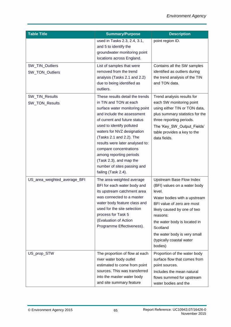
Environment Agency
Report Reference: UC10943.07/16426-0 November 2015
© Environment Agency 2015 65
Table Title Summary/Purpose Description
used in Tasks 2.3, 2.4, 3.1,
and 5 to identify the
groundwater monitoring point
locations across England.
point region ID.
SW_TIN_Outliers
SW_TON_Outliers
List of samples that were
removed from the trend
analysis (Tasks 2.1 and 2.2)
due to being identified as
outliers.
Contains all the SW samples
identified as outliers during
the trend analysis of the TIN
and TON data.
SW_TIN_Results
SW_TON_Results
These results detail the trends
in TIN and TON at each
surface water monitoring point
and include the assessment
of current and future status
used to identify polluted
waters for NVZ designation
(Tasks 2.1 and 2.2). The
results were later analysed to:
compare concentrations
among reporting periods
(Task 2.3), and map the
number of sites passing and
failing (Task 2.4).
Trend analysis results for
each SW monitoring point
using either TIN or TON data,
plus summary statistics for the
three reporting periods.
The ‘Key_SW_Output_Fields’
table provides a key to the
data fields.
US_area_weighted_average_BFI The area-weighted average
BFI for each water body and
its upstream catchment area
was connected to a master
water body feature class and
used for the site selection
process for Task 5
(Evaluation of Action
Programme Effectiveness).
Upstream Base Flow Index
(BFI) values on a water body
level.
Water bodies with a upstream
BFI value of zero are most
likely caused by one of two
reasons:
the water body is located in
Scotland
the water body is very small
(typically coastal water
bodies)
US_prop_STW The proportion of flow at each
river water body outlet
estimated to come from point
sources. This was transferred
into the master water body
and site summary feature
Proportion of the water body
surface flow that comes from
point sources.
Includes the mean natural
flows summed for upstream
water bodies and the

Environment Agency
Report Reference: UC10943.07/16426-0 November 2015
© Environment Agency 2015 66
Table Title Summary/Purpose Description
classes which were used as
part of the site selection
process for Task 5
(Evaluation of Action
Programme Effectiveness).
upstream flow coming from
point sources (both in
ML/day).
Table B.3 Metadata containing descriptions and a summary/purpose for each
Geodatabase feature class included in the final File Geodatabase
Class Title Summary/Purpose Description
Current_krige
Future_Krige
Difference_krige
TIN_1km_krige
These feature classes were
used to create several maps of
England representing the
current and future TIN
concentrations from the kriging
process and the difference
between the two (Task 3.1).
The TIN_1km_krige feature
class is the final results output
from the kriging analysis, from
which the other three feature
classes were created.
These point feature classes
represent the interpolated TIN
concentrations for every 1 km2
grid square in England.
DGWR_HYDROMETRIC
_AREAS_GB_NI_polygon
This feature class of Large
Hydrological Areas was used
predominantly in Task 2.4 for
assessing the trend analysis
results by LHA and in Task 5
for the site selection process.
This feature class represents
all 59 Large Hydrological
Areas (LHAs) in England and
Wales.
Eng_Outline
Wales_1km_grid_Outline
Eng_Wales_Outine
These feature classes were
used for calculating the total
percentage area of England
and Wales designated as
NVZs (Task 6) and as an
outline of England and Wales
for all maps generated.
This feature class contains a
single polygon outline of
England and Wales.
GW_Change_Preceding_T2_3
GW_Change_Previous_T2_3
GW_Max_NO3_Current_T2_3
GW_Mean_NO3_Current_T2_3
These feature classes were
used in Task 2.3 to create
maps of England showing, for
each groundwater monitoring
point analysed: (i) the change
These point feature classes
included the final groundwater
results from the trend analysis
(Task 2.2).
Several fields have been

Environment Agency
Report Reference: UC10943.07/16426-0 November 2015
© Environment Agency 2015 67
Class Title Summary/Purpose Description
in mean NO3 concentration
between the preceding (2006-
07) and current (2013-14)
reporting periods; (ii) the
change in mean NO3
concentration between the
previous (2010-11) and current
(2013-14) reporting periods;
(iii) the maximum NO3
concentration in the current
(2013-14) reporting period; and
(iv) the mean NO3
concentration in the current
(2013-14) reporting period.
included into these results
(easting, northing, check for
water company data and
check for a minimum amount
of data).
Only sites which met the
criteria for Task 2.3 were
included in this feature class.
Rivers_Change_Preceding_T2_3
Rivers_Change_Previous_T2_3
Rivers_Max_NO3_Current_T2_3
Rivers_Mean_NO3_Current_T2_3
These feature classes were
used in Task 2.3 to create
maps of England showing, for
each river monitoring point
analysed: (i) the change in
mean NO3 concentration
between the preceding (2006-
07) and current (2013-14)
reporting periods; (ii) the
change in mean NO3
concentration between the
previous (2010-11) and current
(2013-14) reporting periods;
(iii) the maximum NO3
concentration in the current
(2013-14) reporting period; and
(iv) the mean NO3
concentration in the current
(2013-14) reporting period.
These point feature classes
included the final surface
freshwater results from the
trend analysis (Task 2.2).
Several fields have been
included into these results
(easting, northing, check for
water company data, check for
canals and check for a
minimum amount of data).
Only sites which met the
criteria for Task 2.3 were
included in this feature class.
TRaC_Change_Preceding_T2_3
TRaC_Change_Previous_T2_3
TRaC_Max_NO3_Current_T2_3
TRaC_Mean_NO3_Current_T2_3
These feature classes were
used in Task 2.3 to create
maps of England showing, for
each TraC monitoring point
analysed: (i) the change in
mean NO3 concentration
between the preceding (2006-
07) and current (2013-14)
reporting periods; (ii) the
These point feature classes
included the final transitional
waters results from the trend
analysis (Task 2.2).
Several fields have been
included into these results
(easting, northing, check for
water company data, check for
canals and check for a
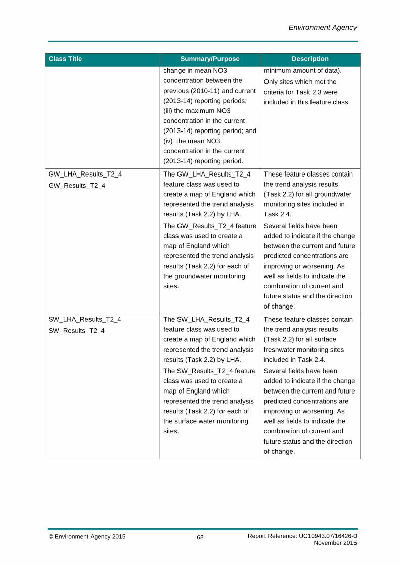
Environment Agency
Report Reference: UC10943.07/16426-0 November 2015
© Environment Agency 2015 68
Class Title Summary/Purpose Description
change in mean NO3
concentration between the
previous (2010-11) and current
(2013-14) reporting periods;
(iii) the maximum NO3
concentration in the current
(2013-14) reporting period; and
(iv) the mean NO3
concentration in the current
(2013-14) reporting period.
minimum amount of data).
Only sites which met the
criteria for Task 2.3 were
included in this feature class.
GW_LHA_Results_T2_4
GW_Results_T2_4
The GW_LHA_Results_T2_4
feature class was used to
create a map of England which
represented the trend analysis
results (Task 2.2) by LHA.
The GW_Results_T2_4 feature
class was used to create a
map of England which
represented the trend analysis
results (Task 2.2) for each of
the groundwater monitoring
sites.
These feature classes contain
the trend analysis results
(Task 2.2) for all groundwater
monitoring sites included in
Task 2.4.
Several fields have been
added to indicate if the change
between the current and future
predicted concentrations are
improving or worsening. As
well as fields to indicate the
combination of current and
future status and the direction
of change.
SW_LHA_Results_T2_4
SW_Results_T2_4
The SW_LHA_Results_T2_4
feature class was used to
create a map of England which
represented the trend analysis
results (Task 2.2) by LHA.
The SW_Results_T2_4 feature
class was used to create a
map of England which
represented the trend analysis
results (Task 2.2) for each of
the surface water monitoring
sites.
These feature classes contain
the trend analysis results
(Task 2.2) for all surface
freshwater monitoring sites
included in Task 2.4.
Several fields have been
added to indicate if the change
between the current and future
predicted concentrations are
improving or worsening. As
well as fields to indicate the
combination of current and
future status and the direction
of change.
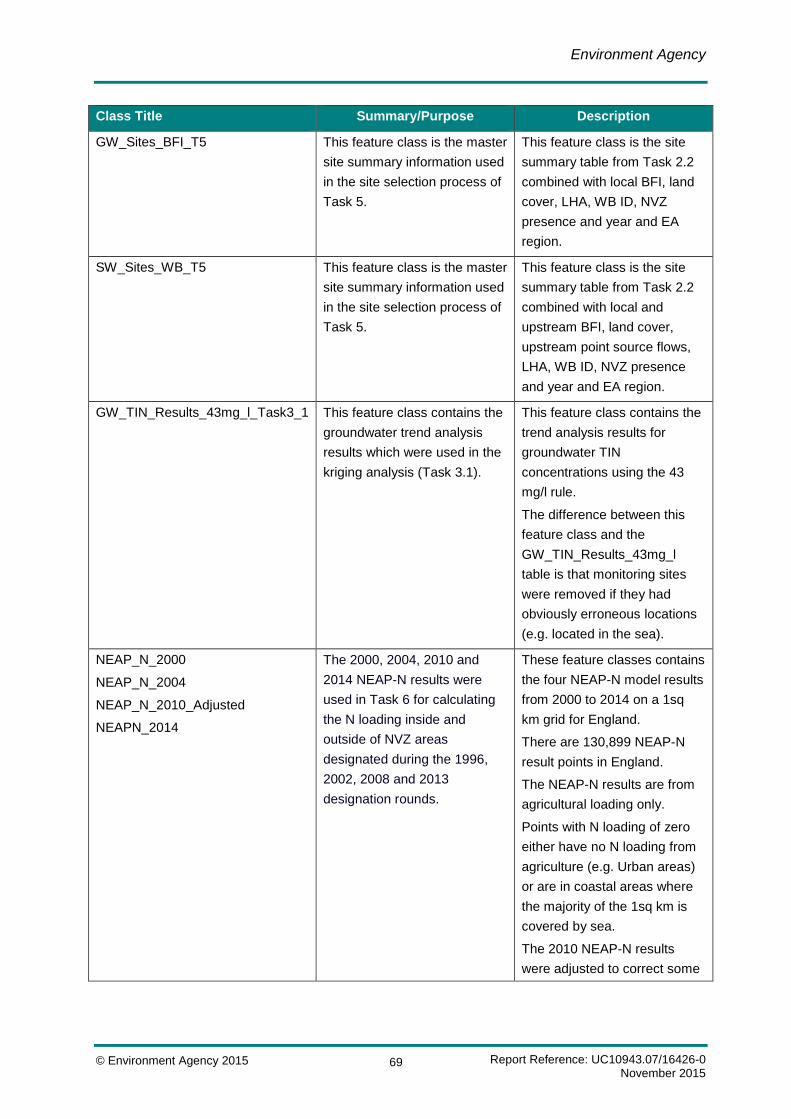
Environment Agency
Report Reference: UC10943.07/16426-0 November 2015
© Environment Agency 2015 69
Class Title Summary/Purpose Description
GW_Sites_BFI_T5 This feature class is the master
site summary information used
in the site selection process of
Task 5.
This feature class is the site
summary table from Task 2.2
combined with local BFI, land
cover, LHA, WB ID, NVZ
presence and year and EA
region.
SW_Sites_WB_T5 This feature class is the master
site summary information used
in the site selection process of
Task 5.
This feature class is the site
summary table from Task 2.2
combined with local and
upstream BFI, land cover,
upstream point source flows,
LHA, WB ID, NVZ presence
and year and EA region.
GW_TIN_Results_43mg_l_Task3_1 This feature class contains the
groundwater trend analysis
results which were used in the
kriging analysis (Task 3.1).
This feature class contains the
trend analysis results for
groundwater TIN
concentrations using the 43
mg/l rule.
The difference between this
feature class and the
GW_TIN_Results_43mg_l
table is that monitoring sites
were removed if they had
obviously erroneous locations
(e.g. located in the sea).
NEAP_N_2000
NEAP_N_2004
NEAP_N_2010_Adjusted
NEAPN_2014
The 2000, 2004, 2010 and
2014 NEAP-N results were
used in Task 6 for calculating
the N loading inside and
outside of NVZ areas
designated during the 1996,
2002, 2008 and 2013
designation rounds.
These feature classes contains
the four NEAP-N model results
from 2000 to 2014 on a 1sq
km grid for England.
There are 130,899 NEAP-N
result points in England.
The NEAP-N results are from
agricultural loading only.
Points with N loading of zero
either have no N loading from
agriculture (e.g. Urban areas)
or are in coastal areas where
the majority of the 1sq km is
covered by sea.
The 2010 NEAP-N results
were adjusted to correct some

Environment Agency
Report Reference: UC10943.07/16426-0 November 2015
© Environment Agency 2015 70
Class Title Summary/Purpose Description
incorrect locations in the
original shapefile.
NVZ_1996_Dissolved
NVZ_2002_Dissolved
NVZ_2008_Dissolved
NVZ_2013_Dissolved
These feature classes were
used to identify the total area
extent of NVZs from the 1996,
2002, 2008 and 2013
designation rounds. This
information was used in Task
6.
These feature classes contain
a single polygon representing
the total extent of NVZs from
the 1996, 2002, 2008 and
2013 designation rounds.
NVZ_1996_T6
NVZ_2002_T6
NVZ_2008_T6
NVZ_2013_T6
These feature classes were
used during Task 6 to identify
the areas covered by each
NVZ type (i.e. SW, GW and
EW (and any areas overlapped
by multiple NVZs from these
designation rounds.
These polygon feature classes
represent all the individual
NVZs put in place during the
1996, 2002, 2008 and 2013
designation rounds.
NVZ_2013_GW_T2_4
NVZ_2013_SW_T2_4
These feature classes were
used to depict the extent of
groundwater and surface water
NVZ designations from the
2013 designation round for two
maps of England in Task 2.4.
These polygon feature classes
represent the total
groundwater and surface water
NVZ extent from the 2013
designation round.
WFD_WB_Cycle1_Final This master water bodies
feature class was used to
identify water body level
attributes for the site selection
process of Task 5.
This feature class is the
master water bodies dataset
which includes the WB
connectivity code, catchment
size, region, local and
upstream BFI, land cover, and
upstream point source flows.

Environment Agency
Report Reference: UC10943.07/16426-0 November 2015
© Environment Agency 2015 71
Appendix C Evaluation of alternative kriging models
C1 Model options
The goal of the kriging analysis was to accurately predict nitrate concentrations across
England at a 1 km2 resolution. This interpolation technique was used to help understand
spatial patterns in the groundwater dataset and predict water quality at unmonitored locations.
A variety of variogram models (Gaussian, exponential, spherical, double-exponential and
exponential-spherical, with and without a nugget variance) and data transformations (log and
power) were explored. Many of these were discarded at an early stage because (i) the
variogram model would not converge, (ii) the model clearly did not capture the shape of the
variogram, or (iii) the interpolated surface displayed an unacceptably high degree of
smoothing.
To explore and illustrate the sensitivity of the kriging results to the choice of data
transformation and variogram, three alternative models were compared in detail.
1. Model 1: an exponential model with a non-zero nugget variance and a log
transformation – a basic initial model;
2. Model 2: a double exponential model with a zero nugget variance and a power
transformation – to mirror the 2013 modelling approach; and
3. Model 3: a nested exponential-spherical model with zero nugget variance and a power
transformation – the preferred model (described in Section 3.4.4 above).
The relative performance of the three models was assessed visually by plotting the observed
nitrate concentrations at the 4,160 individual monitoring points against the predicted values
for the 1 km2 grid cells containing those points. The strength of agreement was then
quantified by calculating (i) the root mean square error (RSME3) and (ii) the percentage of
monitoring points where the level of pollution was categorised correctly (low: 0.00 – 5.65 mg
N/l; medium: 5.65 – 11.29 mg N/l; high: >11.29 mg N/l).
3 The Root Mean Square error (RMSE) is metric that quantifies the differences between the values predicted by a
model (in this case, the interpolated concentrations) and the values actually observed (in this case, the
concentrations estimated from the monitoring data). To enable a fair comparison between models, the RSME
was calculated using the back-transformed model predictions. Observed values <0 and >50 mg N/l were
considered to be outliers arising from unreliable trend analysis and truncated to 0.1 and 50 mg N/l, respectively,
to minimise their influence on the RSME calculation.

Environment Agency
Report Reference: UC10943.07/16426-0 November 2015
© Environment Agency 2015 72
C2 Comparison of results
Table C.1 compares the performance of the three models, as measured by the fit between the
observed and predicted values. For both current and future nitrate concentrations, Model 3
performed substantially better than both Models 1 and 2, having the lowest RSME and the
highest categorisation accuracy. An accuracy of 84-85% is considered to be high, given the
imprecision of the ‘observed’ values (i.e. the 95th percentile estimates at individual monitoring
points), and the fact a single prediction for each grid cell is unable to account for within-cell
variation in nitrate concentrations among neighbouring boreholes.
Table C.1 Comparative kriging performance of alternative variogram models
Time horizon Metric Model 1 Model 2 Model 3
Current (2015) RMSE 6.53 6.12 3.97
Categorisation accuracy 70.2% 71.0% 85.4%
Future (2027) RMSE 9.02 7.64 5.17
Categorisation accuracy 63.2% 70.3% 84.0%
Figure C.1 plots the observed nitrate concentrations at the 4,160 individual monitoring points
against the predicted values for the 1 km2 grid cells containing those points (x-axis truncated
at 0 and 40 mg N/l for clarity). All three models tended to under-predict at locations with high
nitrate concentrations and over-predict at locations with low nitrate concentrations, but this
tendency was much weaker for Model 3.

Environment Agency
Report Reference: UC10943.07/16426-0 November 2015
© Environment Agency 2015 73
Figure C.1 Comparison of observed and predicted nitrate concentrations
Current (2015) concentrations Future (2027) concentrations M
od
el 1
Mo
del 2
Mo
del 3
C3 Justification for the preferred model
Like all interpolation algorithms, kriging has the effect of smoothing the data, and therefore will
always tend to under-estimate the high concentrations and over-estimate the low
concentrations. This is potentially problematic if the interpolated surface displays such a high
degree of smoothing that it (i) fails to represent localised nitrate concentration peaks above
the 11.29 mg N/l pollution threshold or (ii) over-states the level of risk in unpolluted areas. It
was therefore imperative to select a model that was able to predict nitrate concentrations
across England as accurately as possible.
The choice of data transformation appeared to have relatively little influence on the results,
but a power transformation was preferred for consistency with the methodology used for the
2013 NVZ Review (see Environment Agency 2012b).
0
5
10
15
20
25
30
35
40
0 5 10 15 20 25 30 35 40
Pre
dic
ted
TIN
co
nce
ntr
atio
n f
or
grid
ce
ll (m
g N
/l)
Estimated TIN concentration at monitoring point (mg N/l)
0
5
10
15
20
25
30
35
40
0 5 10 15 20 25 30 35 40
Pre
dic
ted
TIN
co
nce
ntr
atio
n f
or
grid
ce
ll (m
g N
/l)
Estimated TIN concentration at monitoring point (mg N/l)
0
5
10
15
20
25
30
35
40
0 5 10 15 20 25 30 35 40
Pre
dic
ted
TIN
co
nce
ntr
atio
n f
or
grid
ce
ll (m
g N
/l)
Estimated TIN concentration at monitoring point (mg N/l)
0
5
10
15
20
25
30
35
40
0 5 10 15 20 25 30 35 40
Pre
dic
ted
TIN
co
nce
ntr
atio
n f
or
grid
ce
ll (m
g N
/l)
Estimated TIN concentration at monitoring point (mg N/l)
0
5
10
15
20
25
30
35
40
0 5 10 15 20 25 30 35 40
Pre
dic
ted
TIN
co
nce
ntr
atio
n f
or
grid
ce
ll (m
g N
/l)
Estimated TIN concentration at monitoring point (mg N/l)
0
5
10
15
20
25
30
35
40
0 5 10 15 20 25 30 35 40
Pre
dic
ted
TIN
co
nce
ntr
atio
n f
or
grid
ce
ll (m
g N
/l)
Estimated TIN concentration at monitoring point (mg N/l)

Environment Agency
Report Reference: UC10943.07/16426-0 November 2015
© Environment Agency 2015 74
There were at least two reasons to expect that the variograms should have a high nugget
variance4, namely:
1. the relatively high level of sampling error in estimates of TIN concentrations at
individual monitoring points; and
2. the tendency for neighbouring boreholes sampling groundwater at different depths to
record very different TIN concentrations.
Including a nugget variance in the variogram models, however, resulted in an unacceptably
high degree of smoothing in the interpolated surfaces. For this reason, a zero nugget model
was preferred.
Having opted for a zero nugget model, a nested formulation was found to be necessary to
fully capture the shape of the variogram. The double exponential model (Model 2), as used for
the 2013 NVZ Review, performed well, but the exponential-spherical model (Model 3) had the
lowest RSME and the highest categorisation accuracy. Model 3 was therefore selected as the
preferred model for kriging current and future 95th percentile TIN concentrations.
4 The nugget variance is the y-intercept of the variogram – i.e. the variance at lag zero. It represents the small-
scale variability in the data, which comprises genuine variation in nitrate concentrations (e.g. variation in water
quality between neighbouring deep and shallow boreholes), and sampling and measurements error (i.e. the error
in the estimated 95th percentile concentration at each monitoring point).