Statistical Field Theory - damtp
76
Statistical Field Theory R R Horgan [email protected] www.damtp.cam.ac.uk/user/rrh December 4, 2014 Contents 1 BOOKS iii 2 Introduction 1 3 Definitions, Notation and Statistical Physics 2 4 The D=1 Ising model and the transfer matrix 7 5 The Phenomenology of Phase Transitions 10 5.1 The general structure of phase diagrams ............. 16 5.1.1 Structures in a phase diagram: a description of Q ... 16 6 Landau-Ginsburg theory and mean field theory 18 7 Mean field theory 22 8 The scaling hypothesis 25 9 Critical properties of the 1D Ising model 28 10 The blocking transformation 29 11 The Real Space Renormalization Group 35 12 The Partition Function and Field Theory 45 13 The Gaussian Model 47
Transcript of Statistical Field Theory - damtp
Statistical Field Theory
www.damtp.cam.ac.uk/user/rrh
December 4, 2014
Contents
1 BOOKS iii
2 Introduction 1
3 Definitions, Notation and Statistical Physics 2
4 The D=1 Ising model and the transfer matrix 7
5 The Phenomenology of Phase Transitions 10
5.1 The general structure of phase diagrams . . . . . . . . . . . . . 16
5.1.1 Structures in a phase diagram: a description of Q . . . 16
6 Landau-Ginsburg theory and mean field theory 18
7 Mean field theory 22
8 The scaling hypothesis 25
9 Critical properties of the 1D Ising model 28
10 The blocking transformation 29
11 The Real Space Renormalization Group 35
12 The Partition Function and Field Theory 45
13 The Gaussian Model 47
i
CONTENTS ii
14 The Perturbation Expansion 52
15 The Ginsberg Criterion for Dc 59
16 Calculation of the Critical Index 61
17 General Ideas 68
17.1 Domains and the Maxwell Construction . . . . . . . . . . . . . . . . . 69
17.2 Types of critical point . . . . . . . . . . . . . . . . . . . . . . . . . . 69
17.3 Hysteresis . . . . . . . . . . . . . . . . . . . . . . . . . . . . . . . . . 72
17.4 Mean Field Theory . . . . . . . . . . . . . . . . . . . . . . . . . . . . 73
1 BOOKS iii
1 BOOKS
(1) “Statistical Mechanics of Phase Transitions” J.M. Yeomans, Oxford ScientificPublications.
(2) “Statistical Physics”, Landau and Lifshitz, Pergammon Press.
(3) “The Theory of Critical Phenomena” J.J. Binney et al., Oxford Scientific Pub-lications.
(4) “Scaling and Renormalization in Statistical Physics” John Cardy, CambridgeLecture Notes in Physics.
(5) “ Quantum and Statistical Field Theory” M. Le Bellac, Clarendon Press.
(6) “Introduction to the Renormalisation Group of Critical Phenomena” P. Pfeutyand G. Toulouse, Wiley. ‘
(*7) “Fluctuation Theory of phase Transitions” Patashinskii and Pokrovskii, Perg-amon.
(*8) “Field Theory the renormalisation Group and Critical Phenomena” D. Amit,McGaw-Hill.
(*9) “Quantum Field Theory of Critical Phenomena” J. Zinn-Justin, OXFORD.
(*10) “Phase Transitions and Critical Phenomena” in many volumes, edited by C.Domb and M. Green/Lebowitz.
(*11) “Statistical Field Theory” Vols I and II, Itzykson and Drouffe, CUP.
Note * means it’s a harder book.
2 INTRODUCTION 1
2 Introduction
A general problem in physics is to deduce the macroscopic properties of a quantumsystem from a microscopic description. Such systems can only be described mathe-matically on a scale much smaller than the scales which are probed experimentallyor on which the system naturally interacts with its environment. An obvious reasonis that systems consist of particles whose individual behaviour is known and alsowhose interactions with neighbouring particles are known. On the other hand ex-perimental probes interact only with systems containing large numbers of particlesand the apparatus only responds to their large scale average behaviour. Statisticalmechanics was developed expressly to deal with this problem but, of course, onlyprovides a framework in which detailed methods of calculation and analysis can beevolved.
These notes are concerned with the physics of phase transitions: the phenomenonthat in particular environments, quantified by particular values of external param-eters such as temperature, magnetic field etc., many systems exhibit singularitiesin the thermodynamic variables which best describe the macroscopic state of thesystem. For example:
(i) the boiling of a liquid. There is a discontinuity in the entropy,
∆S =∆Q
Tc
where ∆Q is the latent heat. This is a first order transition;
(ii) the transition from paramagnetic to ferromagnetic behaviour of iron at the Curietemperature. Near the transition the system exhibits large-range cooperative be-haviour on a scale much larger than the inter-atomic distance. This is an exampleof a second order, or continuous, transition. Scattering of radiation by systems ator near such a transition is anomalously large and is called critical opalescence.This is because the fluctuations in the atomic positions are correlated on a scalelarge compared with the spacing between neighbouring atoms, and so the radiationscattered by each atom is in phase and interferes constructively.
Most of the course will be concerned with the analysis of continuous transitionsbut from time to time the nature of first order transitions will be elucidated. Con-tinuous transitions come under the heading of critical phenomena. It underpinsthe modern approach to non-perturbative studies of field theory and particularlylattice-regularized field theories.
Broadly, the discussion will centre on the following area or observations:
(i) the mathematical relationship between the sets of variables which describe thephysics of the system on different scales. Each set of variables encodes the propertiesof the system most naturally on the associated scale. If we know how to relatedifferent sets then we can deduce the large scale properties from the microscopic
3 DEFINITIONS, NOTATION AND STATISTICAL PHYSICS 2
description. Such mathematical relationships are called, loosely, renormalizationgroup equations, and , even more loosely, the relationship of the physics on onescale with that on another is described by the renormalization group. In factthere is no such thing as the renormalization group, but it is really a shorthand forthe set of ideas which implement the ideas stated above and is best understood inthe application of these ideas to particular systems. If the description of the systemis in terms of a field theory then the renormalization group approach includes theidea of the renormalization of (quantum) field theories and the construction ofeffective field theories;
(ii) the concept of universality. This is the phenomenon that many systems whosemicroscopic descriptions differ widely nevertheless exhibit the same critical be-haviour. That is, that near a continuous phase transition the descriptions of theirmacroscopic properties coincide in essential details. This phenomenon is related tothe existence of fixed points of the renormalization group equations.
(iii) the phenomenon of scaling. The relationship between observables and parametersnear a phase transition is best described by power-law behaviour. Dimensionalanalysis gives results of this kind but often the dimensions of the variables areanomalous. That is, they are different from the obvious or “engineering” dimen-sions. This phenomenon occurs particularly in low dimensions and certainly ford < 4. For example in a ferromagnet at the Curie temperature Tc we find
M ∼ h1δ ,
where M is the magnetization and h is the external magnetic field. Then thesusceptibility, χ = ∂M
∂h, behaves like
χ ∼ h1δ−1.
Since δ > 1, χ diverges as h→ 0. The naive prediction for δ is 3. δ is an exampleof a critical exponent which must be calculable in a successful theory. Thecoefficients of proportionality in the above relations are not universal and are noteasily calculated. However, in two dimensions the conformal symmetry of thetheory at the transition point does allow many of these parameters to be calculatedas well. We shall not pursue this topic in this course.
3 Definitions, Notation and Statistical Physics
All quantities of interest can be calculated from the partition function. We shallconcentrate on classical systems although many of the ideas we shall investigatecan be generalized to quantum systems. Many systems are formulated on a lattice,such as the Ising model, but as we shall see others which have similar behaviour arecontinuous systems such as H20. However, it is useful to have one such model inmind to exemplify the concepts, and we shall use the Ising model in D dimensionsto this end, leaving a more general formulation and notation for later.
3 DEFINITIONS, NOTATION AND STATISTICAL PHYSICS 3
The Ising model is defined on the sites of a D-dimensional cubic lattice, denoted Λ,whose sites are labelled by n = n1e1 + . . . nDeD, where the ei, i = 1, . . . , D are thebasis vectors of a unit cell. With each site there is associated a spin variable σn ∈(1,−1) labelled by n. There is a nearest neighbour interaction and an interactionwith an external magnetic field, h. Then the energy is written as
E(σn) = −J∑n,µ
σnσn+µ, J > 0
H(σn) = E − h∑n
σn,
where µ is the lattice vector from a site to its nearest neighbour in the positivedirection, i.e.,
µ ∈ e1, . . . , eD, er = (0, . . . , 1︸︷︷︸r-thposn
, . . . , 0) . (1)
Here σn is the notation for a configuration of Ising spins. This means a choiceof assignment for the spin at each site of the lattice.
E is the energy of the nearest neighbour interaction between spins and the terminvolving h is the energy of interaction of each individual spin with the imposedexternal field h. H is the total energy. The coupling constant J can, in principle,be a function of the volume V since, in a real system, if we change V it changesthe lattice spacing which generally will lead to a change in the interaction strengthJ . Note that h is under the experimenter’s control and so acts as a probe to allowinterrogation of the system.
We shall use a concise notation where the argument σn is replaced by σ. Thepartition function Z is defined by
Z =∑σ
exp(−βH(σ)) =∑σ
exp(−β(E(σ) − h∑n
σn)) , (2)
The system is in contact with a heatbath of temperature T with β = 1/kT . Theway the expression for Z is written shows that h can be thought of as a chemicalpotential. We shall see that it is conjugate to the magnetization M of the system.The point is that the formalism of the grand canonical ensemble will apply. However,we can recover the results we need directly from (2).
We shall assume that J , the coupling constant in H, depends only on the volumeV of the system. Then for a given T, V and h the equilibrium probability densityfor finding the system in configuration σn is
p(σ) =1
Zexp(−βH(σ)). (3)
Averages over p(σ) will be denoted with angle brackets:
〈O(σ) 〉 =∑σ
p(σ)O(σ) . (4)
3 DEFINITIONS, NOTATION AND STATISTICAL PHYSICS 4
The entropy S is given by
S = −k∑σ
p(σ) log(p(σ))
= −k∑σ
1
Zexp(−βH)(−βH − logZ)
= k(β(U − hM) + logZ),
where
U = 〈E 〉 ≡ internal energy,
M = 〈∑n
σn 〉 ≡ magnetization. (5)
Note that S, U,M are extensive. If two identical systems are joined to make anew system these variables double in value, that is, they scale with volume when allother thermodynamic variables are held fixed. Intensive variables such as densityρ, T, P , retain the same value as for the original system.
Then we havekT logZ = − U + TS + hM = − F, (6)
and hence
F = − 1
βlogZ (7)
where F is the thermodynamic potential appropriate for T, V and h as independentvariables. From now on we shall omit V explicitly since for the Ising model it playsno role of interest.
From (2) directly or from the usual thermodynamic properties of F we have
U − hM = −(∂ logZ∂β
)h
, M = −(∂F
∂h
)T
. (8)
[ Comment: These equations are the same as apply in the grand ensemble formalismfor a gas with h ↔ µ and M ↔ N where µ is the chemical potential and N is thenumber of molecules. The important point is that the external fields which we useto probe the system can be manipulated as general chemical potentials coupled toan appropriate thermodynamic observable which measures the response to changesin the probe field. ]
We also have
δS = −k∑σ
δp log p − k∑σ
p1
pδp
= −k∑σ
δp (− β(E − h∑n
σn)− logZ + 1) .
Note: ∑σ
p = 1 =⇒∑σ
δp = 0 . (9)
3 DEFINITIONS, NOTATION AND STATISTICAL PHYSICS 5
NowU =
∑σ
pE ⇒ δU =∑σ
δpE +∑σ
p δE︸ ︷︷ ︸−P δV
, (10)
and so we deduce the usual thermodynamic identity
dU = TdS − PdV + hdM . (11)
We set dV = 0 from now on. In this case compare with the equivalent relation fora liquid-gas system (e.g., H20):
dU = TdS + hdM Ising model or ferromagnetic system
dU = TdS − PdV liquid-gas system.
In the latter case the density is ρ = N/V where N is the (fixed) number of molecules.We may thus alternatively write
dU = TdS +NP
ρ2dρ , (12)
and we see a strong similarity between the two systems with M ↔ ρ. We shallreturn to this shortly.
The system is translationally invariant and so
M = 〈∑n
σn 〉 = N 〈σ0 〉 , (13)
where N is the number of lattice sites and then 〈σ0 〉 is the magnetization per site.
The susceptibility χ is defined by
χ =
(∂M
∂h
)T
= −(∂2F
∂h2
)T
= kT
(∂2 logZ∂h2
)T
. (14)
From (2) we have
χ/N =∂
∂h
(1
Z∑σ
σ0 e−β (E−h
∑nσn)
)
= β
(∑σ
p(σ) (σ0∑n
σn) − kT
Z
(∂Z∂h
)T
∑σ
p(σ)σ0
).
ButkT
Z
(∂Z∂h
)T
= M = N 〈σ0 〉 , (15)
and so we get
χ/N = β
(∑n
〈σ0 σn 〉 − N〈σ0 〉〈σ0〉)
= β∑n
(〈σ0 σn 〉 − 〈σ0 〉〈σ0 〉) .
3 DEFINITIONS, NOTATION AND STATISTICAL PHYSICS 6
We define the correlation function
G(n, r) = 〈σn σn+r 〉 − 〈σn 〉〈σn+r 〉= 〈σn σn+r 〉c ,
where the subscript c stands for connected. By translation invariance G is indepen-dent of n and we can write
G(r) = 〈σ0 σr 〉 − 〈σ0 〉〈σ0 〉 ,=⇒ χ = βN
∑r
G(r) . (16)
From its definition (16) is is reasonable to see that G(r)→ 0 as r = |r| → ∞. This isbecause we would expect that two spins σ0 and σr will fluctuate independently whenthey are far apart and so their joint probability distribution becomes a product ofdistributions for the respective spins:
p(σ0, σr) −→ p(σ0)p(σr) =⇒ 〈σ0 σr 〉 −→ 〈σ0 〉〈σ0 〉 as r →∞ . (17)
Consider an external field hn which depends also on n. Then the magnetic interac-tion term is
−∑n
hn σn . (18)
If we follow the same algebra as for χ above we see that
βG(r) =
(∂
∂hr
)T
〈σ0 〉 . (19)
Physically, G(r) tells us the response of the average magnetization at site 0 to asmall fluctuation in the external field at site r. This is a fundamental object sinceit reveals in detail how the system is affected by external probes. We would expectG(r) → 0 as r → ∞ since we expect the size of such influences to die away withdistance. This should certainly be true for a local theory. We shall see that in manycases we can parameterize the large-r behaviour of G by
G(r) ∼
1
rD−2+ηr ξ ,
ξe−r/ξ
(ξr)(D−1)/2 r ξ ,
(20)
where ξ is an important fundamental length in the theory called the correlationlength. The exponent (D − 2 + η) will be explained. The (D − 2) contribution canbe deduced by dimensional analysis but η, which is an anomalous dimension is anon-trivial outcome of the theory.
For large ξ 1 we have, from above,
χ ∝∑r
G(r) ∼∫r<ξ
dDr1
rD−2+η= ξ2−η
∫u<1
dDu1
uD−2+η∼ ξ2−η . (21)
4 THE D=1 ISING MODEL AND THE TRANSFER MATRIX 7
4 The D=1 Ising model and the transfer matrix
The Ising model is only soluble in D=1,2 and the D = 2 solution is a clever piece ofanalysis. To discuss the concepts which will be relevant to all the models we studyit is useful to investigate the D = 1 model which can be used to highlight the ideas.Note that models in D = 1 are not trivial and many models have been studied indepth.
The expression for Z (2) in D = 1 can be written as follows
Z =∑
σi=±1 ∀i
N−1∏i=0
exp β(Jσiσi+1 +
1
2h (σi + σi+1)
).
Note that the magnetic field term has been trivially rearranged. Now observe thatthis expression can be written as the trace over a product of N 2× 2 matrices:
Z =∑
σi=±1 ∀iWσ0σ1Wσ1σ2Wσ2σ3 . . .WσN−1σ0 , (22)
where the periodic boundary condition σN = σ0 has been used. The matrix W isidentified by comparing these two alternative ways of expressing Z. We find
Wσσ′ = exp β(Jσσ′ +
1
2h (σ + σ′)
).
Evaluating with σ, σ′ = ±1 gives
W =
(µz z−1
z−1 µ−1z
), (23)
whereµ = eB and z = eK B = βh K = βJ.
Thus from eqn. (22)
Z = Tr(WN
),
and henceZ = λN+ + λN− ,
where λ+ and λ− are the eigenvalues of W with λ+ > λ−. For N large the first termdominates and we find that
Z = λN+ .
Hence from eqn. (23) we have
λ2 − (2z cosh B)λ + (z2 − z−2) = 0
=⇒λ+ =
[z cosh B +
√z2 sinh2 B + z−2
]. (24)
W is know as the transfer matrix and is very important in many theoreticalanalyses. In higher dimensions it is a very large matrix indeed but a similar anal-ysis goes through and the partition function is still given in terms of the largest
4 THE D=1 ISING MODEL AND THE TRANSFER MATRIX 8
eigenvalue. In fact, we need know only the few largest eigenvalues to determine allthe observable thermodynamic variables. However, for a very large and even sparsematrix this can be a daunting task.
The free energy is then given by F = − kTN log λ+. Note that F is extensivei.e., it is proportional to N . This is, however, only true as N → ∞ (otherwise λ−contributes a term) which shows that the thermodynamic limit is necessary and Nmust be large enough that (λ−/λ+)N is negligibly small.
The magnetization per site M/N is given by
M/N = kT
(∂ log λ+
∂h
)T
=eK sinh B√
e2K sinh2 B + e−2K. (25)
From now on we use M for magnetization per site, i.e., formerly M/N . In order tokeep translation invariance but work with a finite but large number of spins N weshall use periodic boundary conditions. We may then consider the infinite volumelimit N →∞.
The magnetization is given by
M = 〈σp 〉 =1
Z∑σ
Wσ0σ1 . . . Wσp−1σp σpWσpσp+1 . . . WσN−1σ0 ,
=Tr (W p SWN−p)
Tr (WN)=
Tr (SWN)
Tr (WN).
where S is the matrix
S =
(1 00 −1
),
We see explicitly that M is independent of the choice of p because of translationinvariance encoded by the trace. Let
W e± = λ± e± ,
P = ( e+, e− ) .
Then we write
W = P ΛP−1 Λ =
(λ+ 00 λ−
), (26)
and so
M =Tr (P−1SPΛN)
Tr (ΛN). (27)
Now
ΛN =
(λN+ 00 λN−
)=⇒ Tr (ΛN) = λN+ + λN− .
P is an orthogonal matrix and has the form
P =
(cos φ − sin φsin φ cos φ
), cot 2φ = e2K sinh B .
4 THE D=1 ISING MODEL AND THE TRANSFER MATRIX 9
Then
P−1SP =
(cos 2φ − sin 2φ− sin 2φ − cos 2φ
)and so from (27)
M =(λN+ − λN− ) cos 2φ
λN+ + λN−→ cos 2φ as N → ∞ .
This is the result we have already derived in (25). In the limit N →∞
ΛN → λN+
(1 00 0
),
a result we shall use below.
We now calculate G(r) and so first look at the two spin expectation value:
〈σ0 σr 〉 =1
Z∑σ
σ0Wσ0σ1 . . . Wσr−1σr σrWσrσr+1 . . . WσN−1σ0 ,
=Tr (SW rSWN−r)
Tr (WN),
where we have used translation invariance. Then immediately
〈σ0 σr 〉 =Tr (P−1SPΛrP−1SPΛN−r)
λN+=
Tr
[(cos 2φ − sin 2φ− sin 2φ − cos 2φ
)(λr+ 00 λr−
)(cos 2φ − sin 2φ− sin 2φ − cos 2φ
)(λ−r+ 00 0
)], (28)
where the N →∞ limit has been taken. Then have
〈σ0 σr 〉 = cos2 2φ + sin2 2φ
(λ−λ+
)r(29)
We define
ξ = 1/ log (λ+/λ−) =⇒
G(r) = 〈σ0 σr 〉c = 〈σ0 σr 〉 − 〈σ0 〉〈σr 〉︸ ︷︷ ︸M2
=⇒
G(r) = sin2 2φ e−r/ξ (30)
which is an example of the behaviour quoted above (20) for G(r). The importantpoint is that in most models there is a unique correlation length and it is given by
ξ = 1/ log (λ1/λ2)
where λ1 ≥ λ2 are the two largest eigenvalues of the transfer matrix. It is possiblethat there is more than one relevant correlation length e.g. ξ′ = 1/ log (λ1/λ3)but this depends on the physics being investigated and we shall not refer to thisextension further. The mass gap m of the theory is the inverse correlation lengthm = 1/ξ. We shall see that a large class of the phase transitions we will be studyingare connected with the limit ξ → ∞ (or m → 0). This, of course, means λ2 λ1,i.e., the maximum eigenvalue of the transfer matrix is degenerate.
5 THE PHENOMENOLOGY OF PHASE TRANSITIONS 10
5 The Phenomenology of Phase Transitions
Statistical systems in equilibrium are described by macroscopic, thermodynamic,observables which are functions of relevant external parameters, e.g., temperature,T, pressure, P, magnetic field, h. These parameters are external fields (they maybe x, t dependent) which influence the system and which are under the control ofthe experimenter.
the observables conjugate to these fields are:
entropy S conjugate to temperature Tvolume V conjugate to pressure Pmagnetization M conjugate to mag. field h
Of course V and P may be swapped round: either can be viewed as an externalfield. More common thermodynamic observables are the specific heats at constantpressure and volume, respectively CP and CV ; the bulk compressibility, K; and theenergy density, ε.
Equilibrium for given fixed external fields is described by the minimum of therelevant thermodynamic potential:
Legendre TransformationInternal energy, U for fixed S,VHelmholz free energy, F for fixed T,V: F = U − TS, T = (∂U/∂S)VGibbs free energy, G for fixed T,P: G = F + PV, P = − (∂F/∂V )TEnthalpy H for fixed S,P: H = U + PV, P = − (∂U/∂V )S
A phase transition occurs at those values of the external fields for which oneor more observables are singular. This singularity may be a discontinuity or adivergence. The transition is classified by the nature of the typical singularity thatoccur. Different phases of a system are separated by phase transitions.
Broadly speaking phase transitions fall into two classes:
(1) 1st order
(a) Singularities are discontinuities.
(b) Latent heat may be non-zero.
(c) The correlation length is finite: ξ <∞.
(d) Bodies in two or more different phases may be in equilibrium at the transitionpoint. E.g.,
(i) the domain structure of a ferromagnet;
5 THE PHENOMENOLOGY OF PHASE TRANSITIONS 11
(ii) liquid-solid mixture in a binary alloy: the liquid is richer in one componentthan is the solid;
(e) the symmetries of the phases on either side of a transition are unrelated.
(2) 2nd and higher order: continuous transitions
(a) Singularities are divergences. An observable itself may be continuous or smoothat the transition point but a sufficiently high derivative with respect to an ex-ternal field is divergent. C.f., in a ferromagnet at T = Tc
M ∼ h1δ , χ =
(∂M
∂h
)T
∼ h1δ−1.
(b) There are no discontinuities in quantities which remain finite through thetransition and hence the latent heat is zero.
(c) The correlation length diverges: ξ →∞.
(d) There can be no mixture of phases at the transition point.
(e) The symmetry of one phase, usually the low-T one, is a subgroup of thesymmetry of the other.
An order parameter, Ψ, distinguishes different phases in each of which it takesdistinctly different values. Loosely a useful parameter is a collective or long-rangecoordinate on which the singular variables at the phase transition depend. Ψ isgenerally an intensive variable.
In a ferromagnet the spontaneous magnetization per unit volume at zero field,M(T ), is such an order parameter, i.e.,
M(T ) = limh→0+
M(h, T )
then |M(T )| = 0 for T ≥ Tc, and |M(T )| > 0 for T < Tc.
Note: =(T − Tc)12 will not do.
Ψ is not necessarily a scalar, but in general it is a tensor and is a field of the ef-fective field theory which describes the interactions of the system on macroscopicscales (i.e., scales much greater than the lattice spacing). The idea of such effec-tive field theories is common to many areas of physics and is a natural product ofrenormalization group strategies.
Examples
(1) The ferromagnet in 3 dimensions.
The ferromagnet can be modelled by the Ising model defined in the previous section.
H = −J∑n,µ
σnσn+µ − h∑n
σn,
5 THE PHENOMENOLOGY OF PHASE TRANSITIONS 12
The order parameter is the magnetization per unit volume.
M =1
V
∑n
σn, V = Na3
where N is the number of sites in the lattice and a is the lattice spacing. Note, thatwhilst the σn are discrete, M is a continuous variable in the limit N, V →∞.
Note: from now on we use the symbol M now to mean magnetization per unitvolume
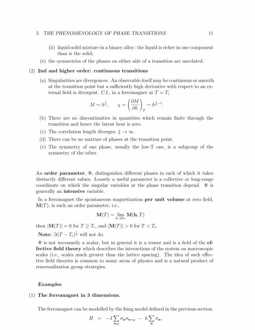
Ising model in two dimensions.Well above the critical temper-ature Tc = 2/ log(1 +
√2) ∼
2.27. Note that the total mag-netization is essentially zero.The theory is paramagnetic.
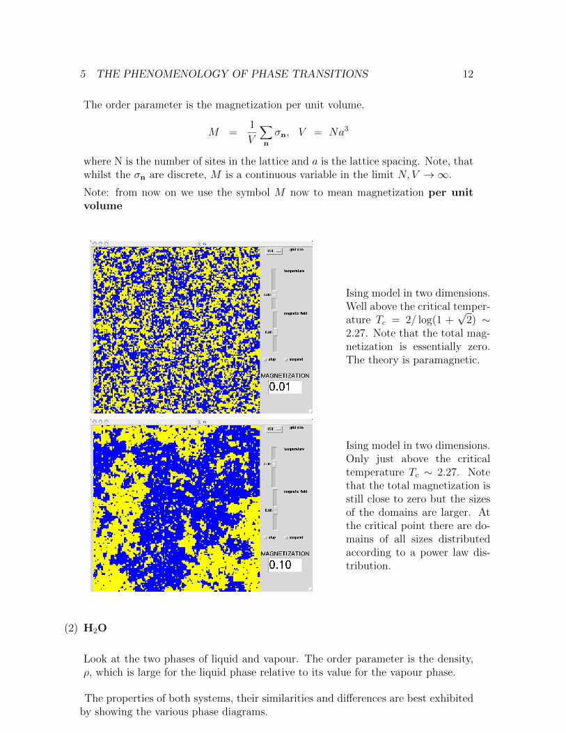
Ising model in two dimensions.Only just above the criticaltemperature Tc ∼ 2.27. Notethat the total magnetization isstill close to zero but the sizesof the domains are larger. Atthe critical point there are do-mains of all sizes distributedaccording to a power law dis-tribution.
(2) H2O
Look at the two phases of liquid and vapour. The order parameter is the density,ρ, which is large for the liquid phase relative to its value for the vapour phase.
The properties of both systems, their similarities and differences are best exhibitedby showing the various phase diagrams.
5 THE PHENOMENOLOGY OF PHASE TRANSITIONS 13
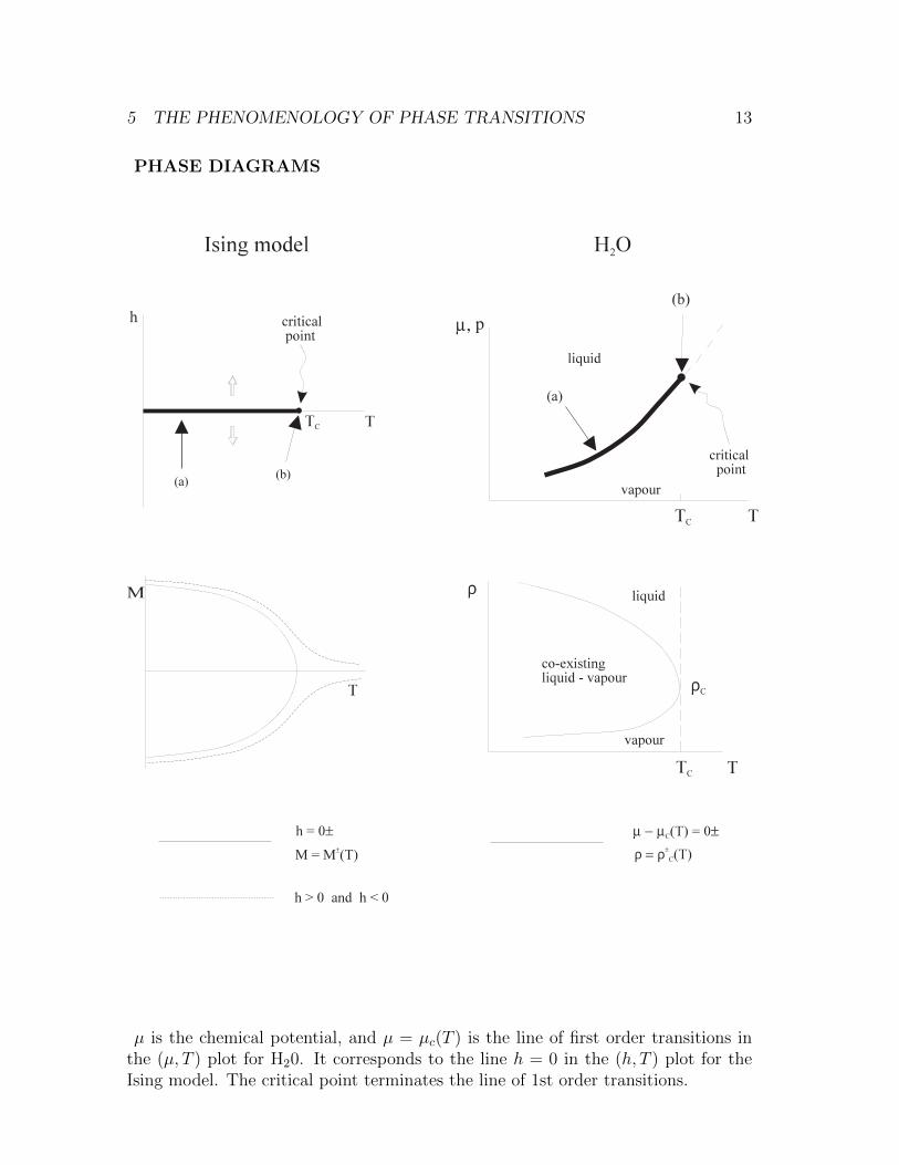
PHASE DIAGRAMS
µ is the chemical potential, and µ = µc(T ) is the line of first order transitions inthe (µ, T ) plot for H20. It corresponds to the line h = 0 in the (h, T ) plot for theIsing model. The critical point terminates the line of 1st order transitions.
5 THE PHENOMENOLOGY OF PHASE TRANSITIONS 14
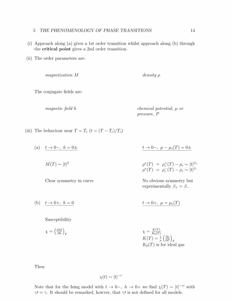
(i) Approach along (a) gives a 1st order transition whilst approach along (b) throughthe critical point gives a 2nd order transition.
(ii) The order parameters are:
magnetization M density ρ
The conjugate fields are:
magnetic field h chemical potential, µ orpressure, P
(iii) The behaviour near T = Tc (t = (T − Tc)/Tc)
(a) t→ 0−, h = 0± t→ 0−, µ− µc(T ) = 0±
M(T ) ∼ |t|β ρ∗(T ) = ρ+c (T )− ρc ∼ |t|β+
ρ∗(T ) = ρ−c (T )− ρc ∼ |t|β−
Clear symmetry in curve No obvious symmetry butexperimentally β+ = β−
(b) t→ 0+, h = 0 t→ 0+, µ = µc(T )
Susceptibility
χ =(∂M∂h
)T
χ = K(T )K0(T )
K(T ) = 1ρ
(∂ρ∂P
)T
K0(T ) is for ideal gas
Then
χ(t) ∼ |t|−γ
Note that for the Ising model with t → 0−, h → 0+ we find χ(T ) ∼ |t|−γ′ withγ′ = γ. It should be remarked, howver, that γ′ is not defined for all models.
5 THE PHENOMENOLOGY OF PHASE TRANSITIONS 15
(c) t = 0, h→ 0+ t = 0, µ− µc → 0+
M ∼ h1δ ρ− ρc ∼ (µ− µc)
1δ
β, γ, δ are examples of critical exponents.
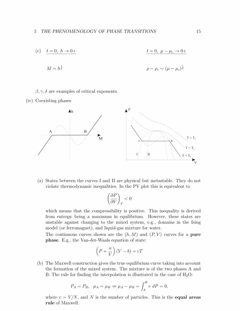
(iv) Coexisting phases
(a) States between the curves I and II are physical but metastable. They do notviolate thermodynamic inequalities. In the PV plot this is equivalent to(
∂P
∂V
)T
< 0
which means that the compressibility is positive. This inequality is derivedfrom entropy being a maximum in equilibrium. However, these states areunstable against changing to the mixed system, e.g., domains in the Isingmodel (or ferromagnet), and liquid-gas mixture for water.
The continuous curves shown are the (h,M) and (P, V ) curves for a purephase. E.g., the Van-der-Waals equation of state:(
P +a
V
)(V − b) = cT
(b) The Maxwell construction gives the true equilibrium curve taking into accountthe formation of the mixed system. The mixture is of the two phases A andB. The rule for finding the interpolation is illustrated in the case of H2O:
PA = PB, µA = µB ⇒ µA − µB =∫ B
Av dP = 0,
where v = V/N , and N is the number of particles. This is the equal areasrule of Maxwell.
5 THE PHENOMENOLOGY OF PHASE TRANSITIONS 16
5.1 The general structure of phase diagrams
A thermodynamic space, Y , is some region in an s-dimensional real vector spacespanned by field variables y1, . . . , ys (e.g., P, V, T, µ, . . .). In Y there will be pointsof two, three, etc. phase coexistence (c.f. A and B in H2O plot above), togetherwith critical points, multicritical points, critical end points, etc.. Q is the totalityof such points. The phase diagram is the pair (Y,Q).
Points of a given type lie in a smooth manifold, M , say. The codimension, κ, ofthese points is defined by
κ = dim(Y )− dim(M).
E.g., two-phase points have κ = 1; critical points (points that terminate two phaselines) have κ = 2.
There do not exist any simple rules for constructing geometrically all acceptablephase diagrams, (Y,Q): we cannot easily construct all the phase diagrams whichcould occur naturally.
5.1.1 Structures in a phase diagram: a description of Q
I assume that there are c components in the system, and hence there are (c + 1)external fields: µ1, . . . , µc, T . Then dim(Y ) = (c+ 1).
Manifolds of multiphase coexistence.
The Gibbs phase rule states that the coexistence of m phases in a system withC components has
f = c+ 2−m
where f is the dimension of the manifold of m-phase coexistence.
proof: dim(Y ) = (c+ 1) and hence the manifold has codimension κ = (c+ 1− f).But κ = (m − 1) since κ external fields must be tuned to bring about m-phasecoexistence.
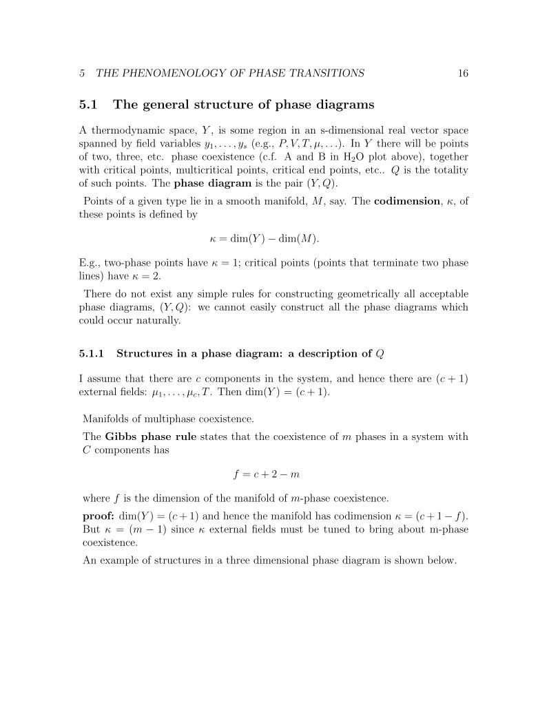
An example of structures in a three dimensional phase diagram is shown below.
5 THE PHENOMENOLOGY OF PHASE TRANSITIONS 17
A tricritical point has κ = 4. Its nature is most easily seen first in three dimen-sions. This is already a special case since we can only be sure it will appear infour dimensions. We suppose we have taken the appropriate cross-section of the 4Dspace. this often occurs naturally since some of the parameters are naturally setto the special values necessary to show up the tricritical point: e.g., by symmetryconsiderations.
The hatched surfaces are 1st-order surfaces: surfaces of two phase coexistence. Thusthe 1st order line in 2D is really a line of triple points (three phase coexistence) inhigher dimensions.
6 LANDAU-GINSBURG THEORY AND MEAN FIELD THEORY 18
6 Landau-Ginsburg theory and mean field theory
The Landau-Ginsburg theory is a phenomenological theory describing all types ofphase transition which can be derived from the more complete theory. It is a classicalapproach which breaks down in its simple form for low dimensions. However, itcan be used for developing the structure of phase transitions and phase diagrams.Landau theory gives the correct prediction for critical indices in dimensions D > Dc,where Dc is a critical dimension which is different for different kinds of critical point.E.g., for an ordinary critical point Dc = 4, and for a tricritical point Dc = 3.
Mean field theory is a method of analysing systems in which the site variable (spinetc.) is assumed to interact with the mean field of the neighbours with which itcouples. In a spin model each of the neighbouring spins has the value of the meanmagnetisation per spin, M. The problem now reduces to that of a single spin inan external field and can easily be solved. By demanding that the mean value ofthe spin in question is M the solution yields a non-linear equation expressing thisassumption of self-consistency and from which M can be calculated as a function ofT. The approximation of the method is that it ignores fluctuations in the spins abouttheir mean. It will turn out that Landau theory suffers from the same deficiency aswe shall demonstrate. Mean field theory and Landau theory give the same, classical,predictions for critical exponents.
Let the order parameter be M . Expand the equilibrium free energy per unitvolume, A(T,M), as
A = A0 +1
2A2M
2 +1
4A4M
4 +1
6A6M
6 + . . . , (31)
with A2 ∝ (T − Tc), A2 = a2(T − Tc), when |T − Tc| is small. Note that A(T,M) isthe appropriate thermodynamic potential when T,M are the independent variables.
There are no terms with odd powers of M . These can be present in principle but canbe consistently excluded by symmetry considerations if the microscopic Hamiltonianis invariant under M → −M . If odd powers of M are present then generally thetheory has only first order transitions, although higher order transitions cannotbe totally excluded. Tc is a complicated function of the couplings in the original,microscopic, Hamiltonian as are the other coefficients, A2n. It is an assumption thatA2 is analytic in T : an assumption that can only be plausibly justified under certaincircumstances. This assumption as well as others is wrong if the dimension is lowenough.
Equilibrium is given by minimising the appropriate thermodynamic potential, inthis case A:
dA
dM= 0, The Equation of State.
The observable value of the order parameter, M(T ), is the solution of this equation.Then
|M(T )| =∣∣∣∣A2
A4
∣∣∣∣12
(1 +
1
2
A6A2
A24
+ . . .
).
6 LANDAU-GINSBURG THEORY AND MEAN FIELD THEORY 19
Thus as T → Tc
|M(T )| ∼ |T − Tc|12 ⇒ β =
1
2.
We can rewrite the expression for M(T ) as
M(T ) =∣∣∣∣A2
A4
∣∣∣∣12
m(x), where x =A6A2
A24
.
The analysis above is only possible if A4 > 0, in which case A6 only occurs in thecorrection terms. If A4 < 0 then we require A6 > 0 to stabilize the calculation andthe results are different (see below).
A4 > 0
If a field h is applied then the symmetry is broken and
A = A0 − hM +1
2A2M
2 +1
4A4M
4.
At T = Tc (A2 = 0) the condition for equilibrium is
−h+ A4M3 = 0 ⇒ M ∼ h
13 ⇒ δ = 3.
For T > Tc we have (t = (T−Tc)Tc
) the Equation of State (EoS) is
−h+ a2TctM + A4M3 = 0.
Then the susceptibility is given by
χ =
(∂M
∂h
)h=0
=1
a2Tct−1 ⇒ γ = 1.
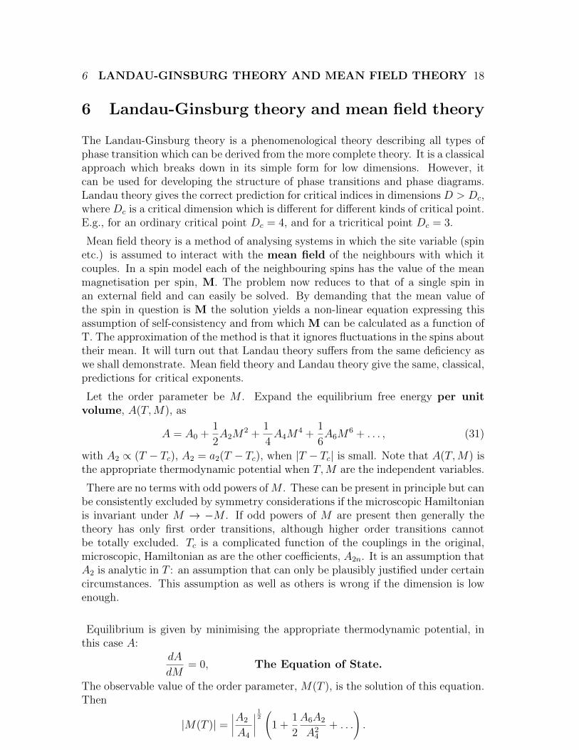
Consider now T < Tc:
The curve of ±M(T ) vs T for h = 0 is a parabola for sufficiently small t followsfrom the EoS
6 LANDAU-GINSBURG THEORY AND MEAN FIELD THEORY 20
A4M3 − a2|T − Tc|M ∼ h , (32)
where A4 is a function of T which does not vanish at T = Tc
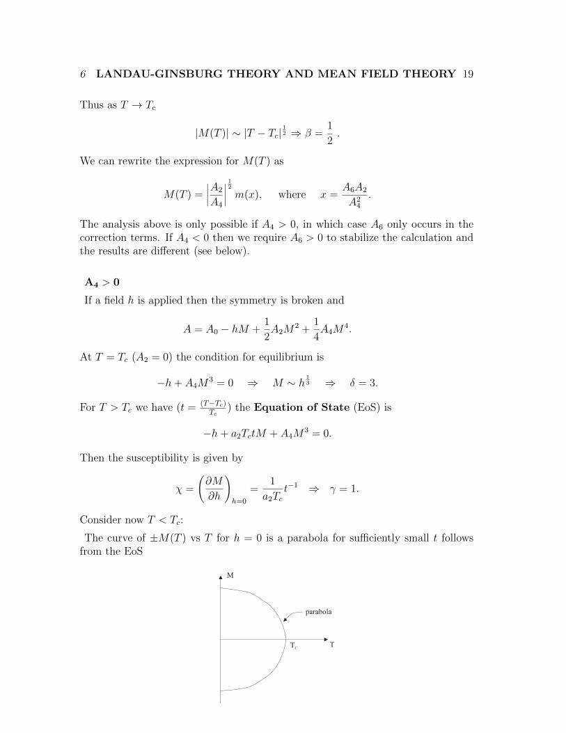
In general the EoS has the form
−a(T )M + b(T )M3 + . . . = h (33)
with a(T ) > 0. Then have
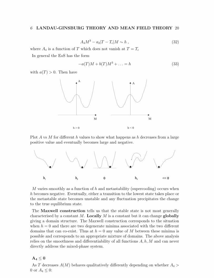
Plot A vs M for different h values to show what happens as h decreases from a largepositive value and eventually becomes large and negative.
M varies smoothly as a function of h and metastability (supercooling) occurs whenh becomes negative. Eventually, either a transition to the lowest state takes place orthe metastable state becomes unstable and any fluctuation precipitates the changeto the true equilibrium state.
The Maxwell construction tells us that the stable state is not most generallycharacterised by a constant M . Locally M is a constant but it can change globallygiving a domain structure. The Maxwell construction corresponds to the situationwhen h = 0 and there are two degenerate minima associated with the two differentdomains that can co-exist. Thus at h = 0 any value of M between these minima ispossible and corresponds to an appropriate mixture of domains. The above analysisrelies on the smoothness and differentiability of all functions A, h,M and can neverdirectly address the mixed-phase system.
A4 ≤ 0
As T decreases A(M) behaves qualitatively differently depending on whether A4 >0 or A4 ≤ 0:
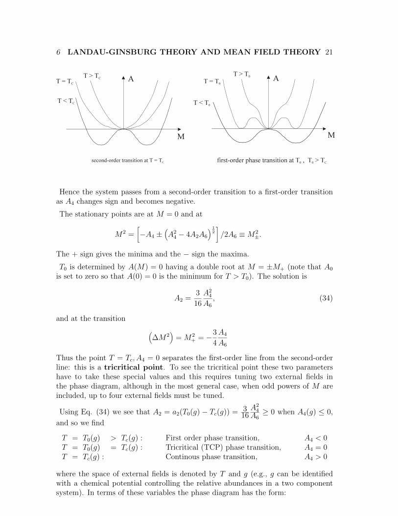
6 LANDAU-GINSBURG THEORY AND MEAN FIELD THEORY 21
Hence the system passes from a second-order transition to a first-order transitionas A4 changes sign and becomes negative.
The stationary points are at M = 0 and at
M2 =[−A4 ±
(A2
4 − 4A2A6
) 12
]/2A6 ≡M2
±.
The + sign gives the minima and the − sign the maxima.
T0 is determined by A(M) = 0 having a double root at M = ±M+ (note that A0
is set to zero so that A(0) = 0 is the minimum for T > T0). The solution is
A2 =3
16
A24
A6
, (34)
and at the transition (∆M2
)= M2
+ = −3
4
A4
A6
Thus the point T = Tc, A4 = 0 separates the first-order line from the second-orderline: this is a tricritical point. To see the tricritical point these two parametershave to take these special values and this requires tuning two external fields inthe phase diagram, although in the most general case, when odd powers of M areincluded, up to four external fields must be tuned.
Using Eq. (34) we see that A2 = a2(T0(g) − Tc(g)) = 316A2
4A6≥ 0 when A4(g) ≤ 0,
and so we find
T = T0(g) > Tc(g) : First order phase transition, A4 < 0T = T0(g) = Tc(g) : Tricritical (TCP) phase transition, A4 = 0T = Tc(g) : Continous phase transition, A4 > 0
where the space of external fields is denoted by T and g (e.g., g can be identifiedwith a chemical potential controlling the relative abundances in a two componentsystem). In terms of these variables the phase diagram has the form:
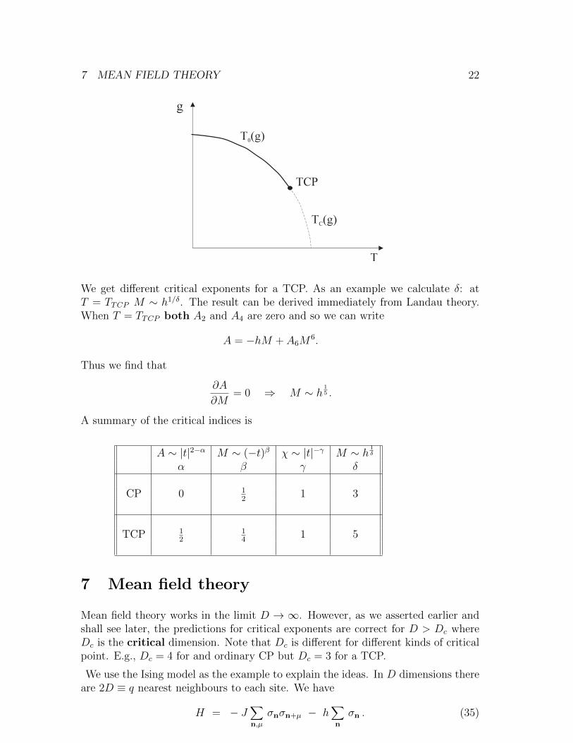
7 MEAN FIELD THEORY 22
We get different critical exponents for a TCP. As an example we calculate δ: atT = TTCP M ∼ h1/δ. The result can be derived immediately from Landau theory.When T = TTCP both A2 and A4 are zero and so we can write
A = −hM + A6M6.
Thus we find that
∂A
∂M= 0 ⇒ M ∼ h
15 .
A summary of the critical indices is
A ∼ |t|2−α M ∼ (−t)β χ ∼ |t|−γ M ∼ h1δ
α β γ δ
CP 0 12
1 3
TCP 12
14
1 5
7 Mean field theory
Mean field theory works in the limit D → ∞. However, as we asserted earlier andshall see later, the predictions for critical exponents are correct for D > Dc whereDc is the critical dimension. Note that Dc is different for different kinds of criticalpoint. E.g., Dc = 4 for and ordinary CP but Dc = 3 for a TCP.
We use the Ising model as the example to explain the ideas. In D dimensions thereare 2D ≡ q nearest neighbours to each site. We have
H = − J∑n,µ
σnσn+µ − h∑n
σn . (35)
7 MEAN FIELD THEORY 23
We write the identity (see Cardy)
σnσn′ = (M + (σn −M)) (M + (σn′ −M)) (36)
and define δσn = (σn−M). Here M is the magnetization per spin. We expand thisexpression and get
σnσn′ = −M2 + M (σn + σn′) + δσn δσn′ . (37)
The mean field approximation consists in ignoring the last term which representsthe interaction between sites of the fluctuations δσ of the spins about their meanvalue. What this really means is that we are asserting that the role of fluctuationsis not important for the quantities we want to calculate. For example, it may bethat their whole effect is just to modify the value of J to some effective value orthey modify overall coefficients, but otherwise the theory gives the same answers forphase structure etc. without explicitly including them.
This assumption is related to the central limit theorem. As D →∞ we expect thatthe magnitude of
〈 δσ0 ( 12D
∑n
δσn) 〉 ∼ 1/√D , n ∈ 2D nearest neighbours of 0 ,
This measures the average interaction of fluctuations between a spin and its nearestneighbours. Thus, the effect of fluctuations becomes negligible for large enough D.How big D must be and how the assumption breaks down is the interesting question.
Then the mean field Hamiltonian H is
H =1
2qJNM2 − (qJM + h)
∑n
σn (38)
and
Z = e−12βqJNM2 ∑
σ
eβ(qJM+h)∑
nσn
= e−12βqJNM2
[2 cosh β(qJM + h)]N . (39)
Note that our discrete Ising spin has been replaced by a continous variable or field:the magnetization M . This is a hint at why many different models are in the sameuniversality class.
The magnetization is given by
M = 〈σ0〉 =
∑σ=±1
σ eβ(qJM+h)σ
∑σ=±1
eβ(qJM+h)σ
= tanh β(qJM + h) . (40)
So
A = F/N = − kT logZ =
= −kT log [2 cosh β(qJM + h)] +1
2qJM2 . (41)
7 MEAN FIELD THEORY 24
The result for M above (40) then also arises from minimizing the free energy A:(∂A
∂M
)T,h
= 0 ⇒ M = tanh β(qJM + h) . (42)
This is the equation of state. For small M,h (i.e., ignoring non-linear terms in hand a few other non-essential terms) we can expand A:
A =
−kT log 2 − 1
βlog
[1 + β2(qJM + h)2/2 + β4(qJM + h)4/24 + . . .
]+
1
2qJM2
= A0(T ) − (βqJ)hM +1
2qJ(1− βqJ)M2 +
1
12qJ(βqJ)3M4 + . . . , (43)
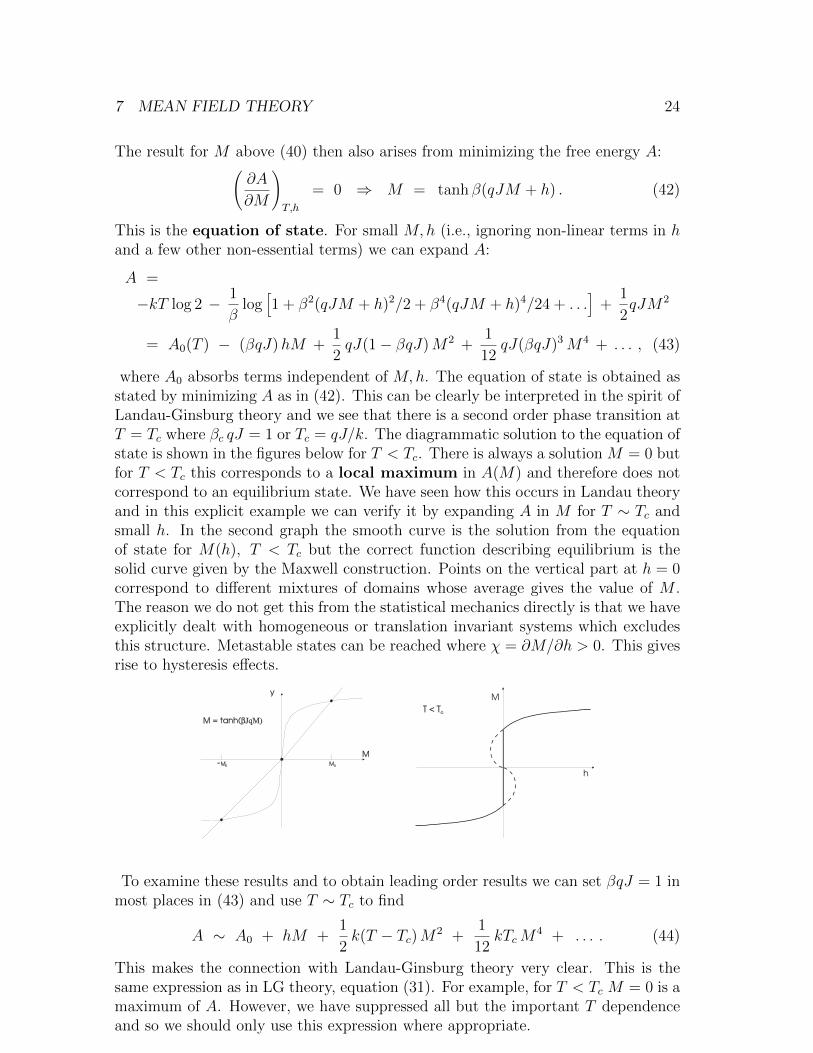
where A0 absorbs terms independent of M,h. The equation of state is obtained asstated by minimizing A as in (42). This can be clearly be interpreted in the spirit ofLandau-Ginsburg theory and we see that there is a second order phase transition atT = Tc where βc qJ = 1 or Tc = qJ/k. The diagrammatic solution to the equation ofstate is shown in the figures below for T < Tc. There is always a solution M = 0 butfor T < Tc this corresponds to a local maximum in A(M) and therefore does notcorrespond to an equilibrium state. We have seen how this occurs in Landau theoryand in this explicit example we can verify it by expanding A in M for T ∼ Tc andsmall h. In the second graph the smooth curve is the solution from the equationof state for M(h), T < Tc but the correct function describing equilibrium is thesolid curve given by the Maxwell construction. Points on the vertical part at h = 0correspond to different mixtures of domains whose average gives the value of M .The reason we do not get this from the statistical mechanics directly is that we haveexplicitly dealt with homogeneous or translation invariant systems which excludesthis structure. Metastable states can be reached where χ = ∂M/∂h > 0. This givesrise to hysteresis effects.
To examine these results and to obtain leading order results we can set βqJ = 1 inmost places in (43) and use T ∼ Tc to find
A ∼ A0 + hM +1
2k(T − Tc)M2 +
1
12kTcM
4 + . . . . (44)
This makes the connection with Landau-Ginsburg theory very clear. This is thesame expression as in LG theory, equation (31). For example, for T < Tc M = 0 is amaximum of A. However, we have suppressed all but the important T dependenceand so we should only use this expression where appropriate.
8 THE SCALING HYPOTHESIS 25
8 The scaling hypothesis
In Landau theory we have
A = A0 − hM +1
2A2M
2 +1
4A4M
4 + . . . ,
and
dA
dM= 0 =⇒
−h+ A2M + A4M3 = 0 ,
where A is the free energy per unit volume. M is, for example, the magnetizationper unit volume in an Ising system or the deviation ρ∗ = ρ − ρc of the density ρfrom its critical value ρc in a liquid.
We have seen how this leads to predictions for critical exponents. However, theseprediction do not always agree with experimentally observed values even thoughthe topological structure of the phase diagram can be well described by the Landauapproach. Because power-law behaviour is still the right form to use in fittingexperiment it suggests an approach based on a form of dimensional analysis or on ascaling formulation.
Suppose we scale units by a factor “k”. Then, since, A is the free energy per unitvolume
A → A′ = k−DA .
[ This means that if the old unit is a and the new unit a′ then a′ = k−1a. E.g.,consider a length expressed in the two kinds of units. We must have
L′a′ = La ⇒ L′ = kL
V ′a′D
= V aD ⇒ V ′ = kDV
]
Denote the dimension of A by [A] so that [A] = −D. Suppose [M ] = DM buta-priori we do not know the value of DM . Note that it is not a general property thatwe can assign a dimension to M . It will only be a useful concept near a continuoustransition. Of course, we can always use standard or “engineering” dimensionalanalysis but here we are proposing something more general. Then
[An] = − (D + nDM) .
The phase transition is caused by A2 changing sign and we assume that A4 > 0(however, see TCP) and so the series can be truncated after M4. We use the ideathat A is an homogeneous function and so we construct dimensionless ratios madeof h (≡ A1), A2, A4:
[h] = − (D +DM), [A2] = − (D + 2DM), [A4] = − (D + 4DM) .
8 THE SCALING HYPOTHESIS 26
Consider hAp22 Ap44 and we find, for DM and D unrelated,
1 + p2 + p4 = 0 1 + 2p2 + 4p4 = 0 =⇒ p2 = − 3
2, p4 =
1
2.
The only dimensionless term is thus
hA1/24
|A2|3/2.
A4 is not particularly interesting: the denominator |A2| is the interesting part. It isnatural to use |A2| here and not A2 since as A2 vanishes we must ensure continuityof expressions. In other words we want continuity of A at T = Tc and will expressthe behaviour for T > Tc, T < Tc as separate functions of |t|, t = (T − Tc).To carry the dimension of A we need to construct a variable with dimension −D.
(a) h = 0. Find|A2|2
A4
∼ |t|2 .
(b) t = 0 =⇒ A2 = 0. Findh4/3
A1/34
.
So, using (a), we can write the singular part of A in its scaling form appropriate forsmall h
A = a|t|2 f><
(bh
|t|3/2
). (45)
The functions f><
apply for t > 0 and t < 0, respectively, with f<(0) = f>(0). Note
that the exponents 2 and 3/2 are universal but a and b are not. The theory willdescribe e.g., both the ferromagnet and H20.
Then
M =
(∂A
∂h
)h→0+
∼ |t|2 1
|t|3/2f ′><
(0+) =⇒
M ∼ |t|1/2 t < 0 f ′<(0+) > 0
M = 0 t > 0 f ′>(0+) = 0
Note that f ′<(0+) = − f ′<(0−) by symmetry. This is evident from our previousdiscussion of Landau theory.
The susceptibility χ is then
χ =
(∂M
∂h
)∼ |t|−1A>
<=⇒ γ = 1 .
A> = ab2f ′′>(0) , A< = ab2f ′′<(0) .
8 THE SCALING HYPOTHESIS 27
We have the specific heat C given by
C = T
(∂2A
∂T 2
)∣∣∣∣∣h=0
.
From (45) find C ∼ t0 =⇒ α = 0
Both A>, A< are non-zero and positive. Clearly, the ratio of A> to A< does notdepend on the non-universal parameter ab2. Thus, in addition to the critical expo-nents, we expect A>/A< to be universal if the functions f>
<are universal. This is
true in Landau theory and we will see that it is true generally.
From (b) above we can also write the singular part of A appropriate for small tand non-zero (positive) h as
A = ch4/3 g><
(1
b
|t|3/2
h
).
A similar analysis to that above pertains.
In this way we reproduce all the critical exponents that we derived before. Thescaling generalizes the approach to accommodate the observed values within thisgeneral framework.
The hypothesis is the postulate that we can write
A = |t|2−α f><
(h
|t|∆
), (46)
from which we associate α with the scaling of the free energy. This form is appro-priate when t is non-zero. Clearly, from above the simple scaling argument givesA ∼ |t|2 ⇒ α = 0. However, we now allow α,∆ to be free parameters.
Following our earlier steps we get
M ∼ |t|β t < 0 , β = 2− α−∆
χ ∼ |t|−γ −γ = 2− α− 2∆
=⇒ α + 2β + γ = 2 scaling relation
This is to be compared with the Rushbrooke inequality deduce from thermodynam-ics: α + 2β + γ ≥ 2 (problem sheet).
Other exponents are calculated with t = 0. Take h > 0 and then we can rewrite
M = (∂A/∂h) ∼ |t|βf ′<
(h
|t|∆
)
= hβ/∆(|t|∆
h
)β/∆f ′<
(h
|t|∆
)︸ ︷︷ ︸
φ
(|t|∆
h
). (47)
9 CRITICAL PROPERTIES OF THE 1D ISING MODEL 28
We assume that limx→0 φ(x) is finite and 6= 0. Then for t = 0
M ∼ h1/δφ(0) =⇒
1/δ =β
∆=
(2− α−∆)
∆=⇒
β δ = ∆ = β + γ scaling relation
On the assumption that the functions defined have suitable limits we have derivedscaling relationships between critical indices. This is because they are ultimatelydependent only on the two independent exponents α and ∆. This has been achievedby invoking a generalized scaling theory which is dimensional analysis but withdimensions which must be predicted by theory. We also see how universalityfor exponents and amplitude ratios (such as A>/A<) arise. This is because verydifferent theories can have order parameters with the same properties. For example,magnetization M and density ρ∗ = (ρ − ρc). The Landau analysis is the same forall such theories which thus fall into universality classes. This will be justified bythe Renormalization Group (RG) analysis.
We shall also see that there is an exponent ν associated with the divergence of thecorrelation length ξ defined by
ξ ∼ |t|−ν t→ 0 .
9 Critical properties of the 1D Ising model
Except in special circumstances there are no phase transitions at non-zero T inone dimension. The entropy S is largest when the system is disordered and itscontribution to F = U −TS dominates the internal energy term U except at T = 0.Hence, the minimum of F always corresponds to a disordered state: a state usuallyassociated with high T in higher dimensional models. In the 1D Ising model there iscritical behaviour as T → 0⇒ Tc = 0. We can see this by computing the correlationlength for h = 0 and low T :
ξ−1 = log(λ+/λ−) = log coth βJ
∼ 2 exp(−2J/kT ) T → 0
⇒ξ ∼ 1
2exp(2J/kT ) T → 0 . (48)
Thus ξ diverges as T → 0 and this signifies a continuous transition at Tc = 0. Theapproach to the transition is actually T/J → 0, h/T → 0, which includes J → ∞at fixed T > 0. Because of this we use t = exp(−4J/kT ) to measure the departurefrom criticality rather than (T − Tc)/Tc (there is a abritary nature to this choice,see later). To encode the magnetic field dependence we use B = h/kT as defined
10 THE BLOCKING TRANSFORMATION 29
before. Then from section 4 equation (25) we find for small t and B
M ∼ B√t+B2
=1√
(t/B2) + 1.
Compare with the form for M given by the scaling hypothesis (47) in the previoussection
M ∼ B1/δ φ
(t∆
B
),
and we read off that δ =∞ and βδ = β + γ = ∆ = 1/2. This gives β = 0, γ = 1/2,and if the scaling relation α + 2β + γ = 2 holds true we find α = 3/2. Also weidentify
φ(x) = 1/√x2 + 1 .
The exponent ν is defined by ξ ∼ t−ν and from above we have
ξ ∼ t−1/2 ⇒ ν = 1/2 .
The exponent η fleetingly referred to before is defined by
G(r) ∼ 1
rD−2+ηr ξ ,
and we have from section (4) equation (30) that G(r) ∼ sin2 2φ in this limit andhence η = 1.
In fact, the definition of t is rather arbitrary and any power of t will do equallywell. This, of course, affects some of the exponents and so the better way to expressthese results is
2− α = γ = ν , β = 0, δ =∞, η = 1 .
Remember the relation for α depends on assuming α + 2β + γ = 2 but becausethe definition of α is tricky in this case, it is not obvious that we can invoke thisrelation. We can calculate the free energy directly from the exact solution and seewhat is going on (see problem sheet 2). This is a pathology of the 1D Ising modelwhich is unusual in this respect.
10 The blocking transformation
The critical properties of a system are governed by the behaviour of degrees offreedom which vary typically on the scale of the correlation length, ξ. Since, ξdiverges at the critical point we are interested in the dynamics of modes whosewavelengths are much larger than a lattice spacing and we would like to find aneffective theory or Hamiltonian which describes the large scale properties of thesystem but which is, itself, defined only in terms of these long-wavelength modes.Effectively, we want to “integrate” out the short-wavelength modes and come upwith a new theory with fewer degrees of freedom but which has the same criticalproperties as the original system.
10 THE BLOCKING TRANSFORMATION 30
We do something like this all the time. Chemists deal with collections of atomsfor which they have a way of describing their interactions and bonding properties.When building a large molecule they generally do not write down Schrodinger’sequation for all the constituent electrons and nuclei and solve from first principles.Instead, they have an effective description in which the atoms are entities whichinteract on a scale larger than the internal atomic scales. Their description is notso elegant as the original Schodinger equation but it is practical and concentrateson addressing the physics relevant to their problem. “Integrating” out the smallwavelength modes gave the atomic bound states in the first place. Again, we treatatomic nuclei as particles with charge and if we want to study atomic physics we donot feel it necessary to solve the nuclear physics of the nucleus at the same time. Weloose information (such as which isotopes are stable etc.) but we do not mind. Ofcourse, if the chemist heats up the molecules a lot, the atoms will eventually ionizeand the electrons and nuclei will become separate particles in a plasma. The atomic– long-range – description is no longer any good.
In statistical systems we “thin” the degrees of freedom using a blocking strategy.This can sometimes be exact but generally is approximate. The hope is that weretain the correct critical properties and phase structure in the new theory. A badblocking scheme will eliminate degrees of freedom that are necessary for criticalbehaviour and the scheme will fail.
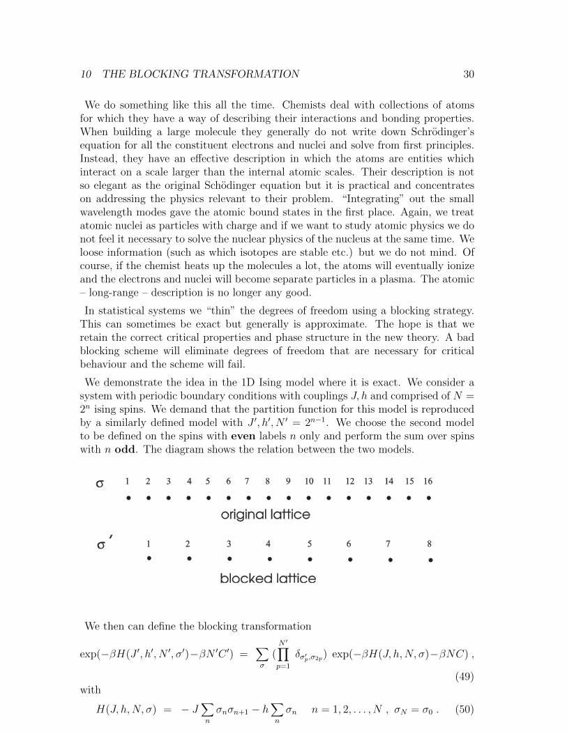
We demonstrate the idea in the 1D Ising model where it is exact. We consider asystem with periodic boundary conditions with couplings J, h and comprised of N =2n ising spins. We demand that the partition function for this model is reproducedby a similarly defined model with J ′, h′, N ′ = 2n−1. We choose the second modelto be defined on the spins with even labels n only and perform the sum over spinswith n odd. The diagram shows the relation between the two models.
We then can define the blocking transformation
exp(−βH(J ′, h′, N ′, σ′)−βN ′C ′) =∑σ
(N ′∏p=1
δσ′p,σ2p) exp(−βH(J, h,N, σ)−βNC) ,
(49)with
H(J, h,N, σ) = − J∑n
σnσn+1 − h∑n
σn n = 1, 2, . . . , N , σN = σ0 . (50)
10 THE BLOCKING TRANSFORMATION 31
We have allowed for an additive constant NC in the partition function which we arealways free to do since it just trivially adds to the free energy. We shall see why it isnecessary below. (Note Yeomans introduces a similar C but mine has the oppositesign to hers – I prefer that C adds to the free energy.)
The lattice spacing in the blocked model is 2 times the original model: a new blockspin σ′p has replaced blocks of two original spins (σ2p−1, σ2p) . The blocking functionthat defines how this is done is denoted T (σ′, σ) and here
T (σ′, σ) =N ′∏p=1
δσ′p,σ2p . (51)
T satisfies the condition ∑σ′
T (σ′, σ) = 1 . (52)
This ensures that the blocked model has the original partition function Z(J, h, C,N):
Z(J ′, h′, C ′, N ′)=∑σ′
exp(−βH(J ′, h′, N ′, σ′)− βN ′C ′)
=∑σ′
∑σ
T (σ′, σ) exp(−βH(J, h,N, σ)− βNC)
=∑σ
exp(−βH(J, h,N, σ)− βNC)
= Z(J, h, C,N)
The volumes of the two systems are the same: they describe the same system. Wedefine the blocking factor b = N/N ′, and the lattice spacing has been scaled byk = b−1 (remember, by definition a′ = k−1a and here a′ = ba so that lengths inlattice units scale as L′ = kL). In the example here b = 2.
This particular form of blocking is called decimation and generally does not workwell but in our soluble model it is exact.
Another blocking strategy might for example be the majority rule where we takeblocks with an odd number 2q + 1 of spins and then b = 2q + 1. The block spin isthen given by
σ′r =
b∑p=1
σn+p∣∣∣∣∣∣b∑
p=1
σn+p
∣∣∣∣∣∣n = (r − 1)b+ 1 r = 1, 2, . . . .
That is, σ′ is the majority sign of the block.
In the example we are considering we note that from (49) that the transfer matrixof the blocked model is the square of that of the original model. So
W ′σ′p σ
′p+1
=∑σ2p+1
δσ′p,σ2pδσ′p+1,σ2p+2Wσ2p σ2p+1Wσ2p+1 σ2p+2
⇒W ′ = W 2 (53)
10 THE BLOCKING TRANSFORMATION 32
It is convenient to define z = eβJ , µ = eβh, c = e−βC . Then from section 4 we have
W = c
(µz z−1
z−1 µ−1z
)(54)
and similarly for W ′. We then have the relation
c′(µ′z′ z′−1
z′−1 µ′−1z′
)= c2
(µz z−1
z−1 µ−1z
)(µz z−1
z−1 µ−1z
). (55)
These are three equations in three unknowns and so there is a solution. Withoutthe introduction of the additive constant C in H this would not be the case. Wefind
c′z′µ′ = c2(z2µ2 + 1/z2) (56)
c′/z′ = c2(µ+ 1/µ) (57)
c′z′/µ′ = c2(z2/µ2 + 1/z2) (58)
The results are best expressed in terms of
x = e−4βJ = 1/z4 , y = e−2βh = 1/µ2 , w = e4βC = 1/c4 .
We then find the recursion relations
x′ =x(1 + y)2
(x+ y)(1 + xy)(59)
y′ =y(x+ y)
(1 + xy)(60)
w′ =w2xy2
(1 + y)2(x+ y)(1 + xy). (61)
These equations are called Renormalization Group equations. They relatethe coupling constants of an original model to those of a similar model which hasdegrees of freedom reduced by a factor b = N/N ′ (b = 2 here) but which givesrise to the same large-scale thermodynamic behaviour. This is clear because thethermodynamic quantities in which we are interested are macroscopic degrees offreedom which are determined from the partition function by differentiating withrespect to J, h.
Notes
(1) The fields J, h couple to long range quantities since they are constants. To obtainthe connected pair correlation function G(r) we introduced a varying field hn butnow we consider this field to vary very slowly on the range of one lattice spacing a.We are ultimately interested only inG(r) for r a and so the blocked model retainsall the required information since only short wavelength degrees of freedom havebeen removed. Their contribution is encoded in the changed coupling constants.
10 THE BLOCKING TRANSFORMATION 33
0.0 0.2 0.4 0.6 0.8
x
0.0
0.2
0.4
0.6
0.8y
RG flows for 1D Ising model
ll
line
of fix
ed
po
ints
fixed point
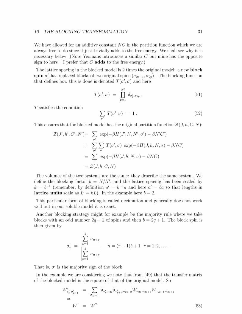
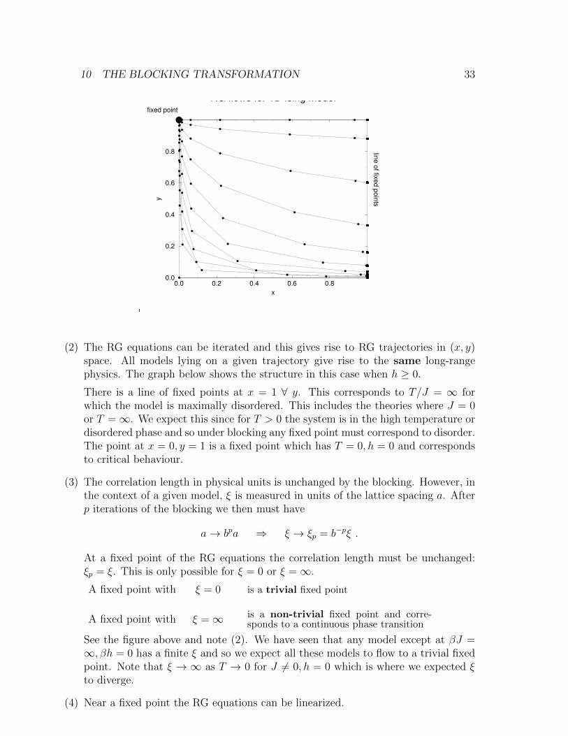
(2) The RG equations can be iterated and this gives rise to RG trajectories in (x, y)space. All models lying on a given trajectory give rise to the same long-rangephysics. The graph below shows the structure in this case when h ≥ 0.
There is a line of fixed points at x = 1 ∀ y. This corresponds to T/J = ∞ forwhich the model is maximally disordered. This includes the theories where J = 0or T =∞. We expect this since for T > 0 the system is in the high temperature ordisordered phase and so under blocking any fixed point must correspond to disorder.The point at x = 0, y = 1 is a fixed point which has T = 0, h = 0 and correspondsto critical behaviour.
(3) The correlation length in physical units is unchanged by the blocking. However, inthe context of a given model, ξ is measured in units of the lattice spacing a. Afterp iterations of the blocking we then must have
a→ bpa ⇒ ξ → ξp = b−pξ .
At a fixed point of the RG equations the correlation length must be unchanged:ξp = ξ. This is only possible for ξ = 0 or ξ =∞.
A fixed point with ξ = 0 is a trivial fixed point
A fixed point with ξ =∞ is a non-trivial fixed point and corre-sponds to a continuous phase transition
See the figure above and note (2). We have seen that any model except at βJ =∞, βh = 0 has a finite ξ and so we expect all these models to flow to a trivial fixedpoint. Note that ξ → ∞ as T → 0 for J 6= 0, h = 0 which is where we expected ξto diverge.
(4) Near a fixed point the RG equations can be linearized.
10 THE BLOCKING TRANSFORMATION 34
(i) x = 1− ε, ∀ y:
ε′ = ε2y
(1 + y)2, y′ = y(1− ε1− y
1 + y)
This gives the line of trivial fixed points defined by ε = 0 ∀ y. The firstequation has no linear term.
(ii) x = ε, y = 1− ρ:
ε′ = 4ε+ . . . , ρ′ = 2ρ+ . . . .
This gives the behaviour in the neighbourhood of the fixed point correspond-ing to the continuous phase transition. The linear transformation is alreadydiagonal with eigenvalues 4 and 2, respectively. It is useful to write theseeigenvalues as powers of b, i.e. we write (b = 2)
ε′ = bλtε , ρ′ = bλhρ , with λt = 2, λh = 1 .
We will see that λt and λh play the role of dimensions associated with x (andhence t) and y (and hence h).
(5) C = 14kT log(w) accumulates the free energy contributed by the degrees of freedom
which are summed over. It appears as an additive constant in the exponent in Z.We consider the free energy per spin and note that it is composed of two distinctparts:
F (J, h, C) = f(J, h) + C
f(J, h) = −kTN
logZ(J, h, C = 0, N) . (62)
Then one iteration of the blocking gives
exp(−βNF (J, h, C)) = exp(−βN ′F (J ′, h′, C ′))
⇒
F (J, h, C) =N ′
NF (J ′, h′, C ′) = b−1F (J ′, h′, C ′) (63)
After p iterations of blocking denote the coupling constants obtained by up =(Jp, hp) and the free energy by F (up, Cp). Then we have
F (u0, C0) = b−pF (up, Cp)
⇒f(u0) = b−pf(up) + b−pCp − C0. (64)
We see that Cp accumulates the contribution to the free energy from the spinswhich have been summed over. From the RG equation (61) for w (take logs of bothsides) we see that
Cp = bCp−1 + b g(up−1) (65)
⇒
b−pCp =p−1∑j=0
b−jg(uj) + C0 , p > 0.
11 THE REAL SPACE RENORMALIZATION GROUP 35
The RG equations thus define the function g(u) by (65) above.
We then have an important equation relating the free energy per spin of the originalmodel to that of the blocked model.
f(u0) = b−pf(up)︸ ︷︷ ︸singular part
+p−1∑j=0
b−jg(uj)︸ ︷︷ ︸inhomog. part
. (66)
with g(u) defined from the RG equation (61). The RHS contains a so-called “singu-lar” part and an inhomogeneous part: the free energy does not transform homoge-neously. Most authors throw away the inhomogeneous part by various arguments.However, (as Ma remarks) this is not correct but can be shown to give the rightanswers and allows us to concentrate on the homogeneous transformation of thesingular part. I will remark on this later.
Near to the fixed point (0, 1) we can expand the RG equation for C (x = ε, y =1− ρ):
w′ =1
4w2 ε ((1− 2ε) + . . .)
⇒C ′ = 2C + kT (
1
4log ε− 1
2log 2− 1
2ε + . . .)
⇒g(u) = kT (
1
8log ε− 1
4ε− 1
4log 2 + . . .) , (67)
where . . . stands for terms higher order in ε, ρ. Note that in this approximationg(u) does not depend linearly on h since there is no linear term in ρ.
In this example we have demonstrated all of the technology of the RG and block-ing. To derive the phenomenon of scaling and to see how critical indices arise wegive a general description of the RG in the next section but draw heavily on theunderstanding gained from this example.
11 The Real Space Renormalization Group
Consider a system defined in D dimensions on a lattice of spacing a with N sitesand with a spin, or field, σr on the r-th site. Note now tht σ can be discrete orcontinuous. The Hamiltonian is defined in terms of a set of operators Oi(σ),e.g., nearest neighbour, next nearest neighbour, multiple groups etc. The generalHamiltonian is
H(u, σ) =∑i
uiOi(σ) , (68)
where the ui are the associated coupling constants and u = (u1, u2, . . .). The parti-tion function is then
Z(u, C,N) =∑σ
exp(−βH(u, σ)− βNC) ,
11 THE REAL SPACE RENORMALIZATION GROUP 36
where C again will accumulate the free energy contribution from summed-over spins.
The RG transformation is defined in terms of a blocking kernel T (σ′, σ)
exp(−βH(u′, σ′)− βN ′C ′) =∑σ
T (σ′, σ) exp(−βH(u, σ)− βNC) .
We have seen an example of a blocking kernel in the previous section. The trans-formation corresponds to summing over a subset of spins to give a model whoseHamiltonian has the same form as the original one (68) but with different couplings.The feature of the transformation is that the new, or blocked, model is defined ona lattice with increased lattice spacing a′ and reduced number of sites N ′.
a → a′ = ba bD = N/N ′ .
In earlier discussion of scaling in section 8 we defined k by a′ = k−1a ⇒ identifyk = b−1 here.
E.g., in the 1D Ising model b = 2. We denote the RG transformation of thecouplings by R, so that under blocking
up → up+1 = R(up) .
We haveZ(up, Cp) = Z(up−1, Cp−1) ∀p > 0 .
Using results from the previous section we have
F (u0, C0) = b−pDF (up, Cp)
⇒f(u0) = b−pDf(up) + b−pDCp − C0, (69)
and hence that
f(u0) = b−pDf(up)︸ ︷︷ ︸singular part
+p−1∑j=0
b−jDg(uj)︸ ︷︷ ︸inhomog. part
. (70)
Again, the inhomogeneous part is the contribution from the degrees of freedom thathave been summed over.
Distances measured in terms of the lattice spacing as a unit also scale with b
r → r′ = b−1r
and in particular this applies to the correlation length ξ → ξ′ = b−1ξ. Remember,the original scale parameter is k = b−1 and so we see that as expected [F ] =−D, [r] = 1, [ξ] = 1.
We might expect that the pair correlation function behaves so that
G(r,u) = G(b−1r,u′) ,
certainly for r a. However, we must also allow for a field rescaling factor whereappropriate. To understand how this works we make the following points:
11 THE REAL SPACE RENORMALIZATION GROUP 37
(1) σ is a dummy variable of summation if it is discrete, or a dummy variable ofintegration if a continuous field. Hence, we can always relabel the blocked field σ′
to be σ.
(2) In addition, we might consider that making a change of summation, or integration,variable is appropriate. In particular, we can scale the field variable. This may notbe useful for a discrete spin since it then does not take values in the original set ofthe unblocked spin but for a field σ ∈ R, for example, it is a possibility.
Combining these ideas and allowing for the field scaling, we write
σ′r = Z(b)σr. (71)
Such a rescaling does not affect the partition function Z, but, of course, to rexpressthe Hamiltonian in standard form then the u′i will be changed in sympathy to absorbapproriate powers of Z. We are always allowed to do this – it is up to us. ChoosingZ(b) has to do with requiring good behaviour for the ui such as the existence of afixed point in the RG equations. It may even be necessary in order to have a simpleanalysis in terms of fixed points and derive a useful RGE.
We then obtain the transformation
G(r,u) = Z(b)2G(b−1r,u′) . (72)
I.e.,
〈σ20σ0〉u = 〈σ′10σ′0〉u′ before relabelling and scaling,
=⇒〈σ20σ0〉u = Z(b)2〈σ10σ0〉u′ after relabelling and scaling.
(73)
Here r′ = 10, r = 20, these are the same physical lengths but in different units:r′a′ = ra.
At a fixed point u∗ we have u∗ = R(u∗) and hence, in particular, that
ξ′ = ξ = b−1ξ ⇒ ξ = 0,∞ .
We are interested in the non-trivial fixed points where ξ = ∞. Such fixed points(f.p.) are associated with continuous phase transitions.
The RG transformation is defined by u→ u′ = R(u). Consider the neighbourhoodof a fixed point u∗ and let
u = u∗ + v , u′ = u∗ + v′ .
with v and v′ small. Then
u∗i + v′i = Ri(u∗ + v) = Ri(u
∗) +∂Ri
∂uj
∣∣∣∣∣u∗
vj
⇒
v′i = Kij(u∗) vj , Kij(u
∗) =∂Ri
∂uj
∣∣∣∣∣u∗
(74)
11 THE REAL SPACE RENORMALIZATION GROUP 38
The transformation linearizes as we saw before in the 1D Ising example. We shallassume that Kij is a symmetric matrix and so is diagonalizable with real eigenvalues.Other situations might occur. Let the eigenvalues of Kij be yα with eigenvectors eα.Then we have
v =∑α
hαeα , v′ =∑α
h′αeα ⇒ h′α = yαhα . (75)
This last equation is really a difference equation and it is better to write it as
h′α = bλαhα , λα =log yαlog b
. (76)
Each λα > 0 determines a critical exponent. The hα are the scaling fields (orvariables) of the system and measure the distance to the f.p. along the eigenvectorseα. We see from the 1D Ising example that when small, (t, h) are scaling fields. Thisis generally the case for all similar models in any dimension.
The Hamiltonian in this region can be rewritten as
H(u) = H(u∗) +∑i
viOi(σ) = H(u∗) +∑i
hαOα(σ)
Oα(σ) =∑i
(eα)iOi(σ) . (77)
The Oα(σ) are scaling operators and are special linear combinations of the oper-ators used to define the Hamiltonian.
(i) λα > 0. |hα| increases under blocking and the system flows away from the fixedpoint in the eα direction. Such a variable is a relevant variable and the associatedoperator Oα(σ) is a relevant operator.
(ii) λα < 0. |hα| decreases under blocking and whatever its initial value it will flow toits fixed point value. Such variables and their associated operators are irrelevant.
(iii) λα = 0. Not considered.
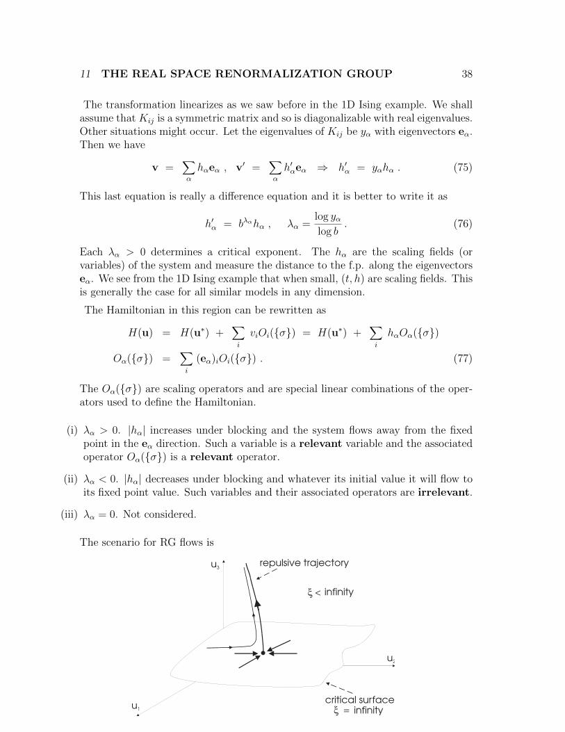
The scenario for RG flows is
11 THE REAL SPACE RENORMALIZATION GROUP 39
The surface of inflowing paths is called the critical surface. On this surface ξ =∞since all models that start in the critical surface are RG equivalent to the fixed pointtheory u = u∗ which has ξ =∞. The corollary is that models that do not lie in thecritical surface have ξ < ∞ since they are on trajectories that ultimately flow to atrivial fixed point which has ξ = 0.
The important points are
(1) Every model in the critical surface is at a continuous phase transition since ξ =∞.
(2) Every such phase transition is RG equivalent to the phase transition described bythe model at the fixed point where u = u∗. In particular, we will expect to see thesame critical behaviour in all these models. This is the idea of universality.
(3) To see the critical behaviour we must tune the external fields so that the couplingsu lie in the critical surface. From before we know that the number we need to tuneis κ, the codimension, of the manifold of transitions. From the RG picture we seethat the number of parameters to be tuned is the number of relevant variables.Thus
κ = number of relevant variables at the fixed point.
(4) The model may contain many couplings but the majority will be irrelevant. If thereare M couplings then the critical surface has dimension M − κ. In general, κ willbe small for practical purposes.
Consider models in the Ising universality class and consider an ordinary criticalpoint which has κ = 2. We have external fields (T, h) and there also may be otherfields which we denote generically by g. The coupling constants are functions of(T, h, g): u(T, h, g).
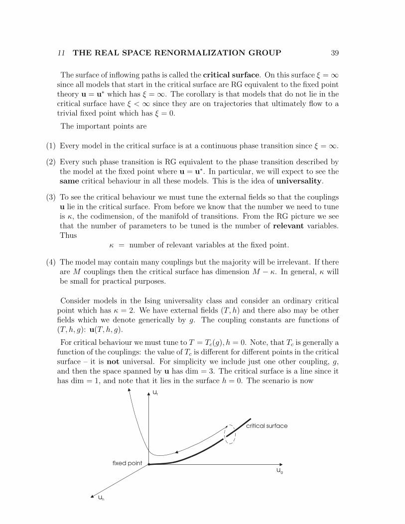
For critical behaviour we must tune to T = Tc(g), h = 0. Note, that Tc is generally afunction of the couplings: the value of Tc is different for different points in the criticalsurface – it is not universal. For simplicity we include just one other coupling, g,and then the space spanned by u has dim = 3. The critical surface is a line since ithas dim = 1, and note that it lies in the surface h = 0. The scenario is now
11 THE REAL SPACE RENORMALIZATION GROUP 40
We have set u = u∗ + (ut, uh, ug) so that when (ut, uh, ug) is small, and hence ulies in the neighbourhood of u∗ (where the RG is linearizable), we have
ut ∼ att , uh ∼ ahh , ug ∼ agg ,
where t and h are relevant scaling fields (as derived earlier), and g represents allthe irrelevant scaling fields. It is simple to define uh = 0 when h = 0 ∀ T, g.
The dotted circle is an example of a set of near critical theories. We follow theblocking history of one such theory.
The RG equations for blocking by a scale factor b are
up → up+1 = R(up) ,
F (up, Cp) = f(up) + Cp
f(u0) = b−pDf(up) +p−1∑j=0
b−jDg(uj) .
(1) Since t = (T − Tc)/Tc and h are small we see that the trajectory passes very closeto u∗ and it passes through the neighbourhood where the RG is linear before itmoves away from the critical surface.
(2) The flow reaches the neighbourhood of u∗ after a finite number of iterations. Thisis because this is all it takes for the irrelevant variables, like g, to become close totheir fixed point values. Let the number of iterations to this point be p. Note thatg essentially measures how far in the critical surface the model is from u∗, and sodetermines the value of p.
Look back at the flows for the 1D Ising model above. I did 1000 iterations percurve but all of them get to (in that case) the trivial fixed points at x = 1 in onlya few steps indicating that p ∼ 5− 10.
Then we haveF (u0, C0) = b−pDF (up, Cp) .
(i) up is in the neighbourhood of u∗ and so we write up = u∗ + (ut, uh, ug).
(ii) I can always choose C0 so that Cp = 0. Of course, this means that C0 = C0(g)since p depends on g. However, C0 is insensitive to (t, h) since these variablesare very small and C0 is certainly well behaved as t, h→ 0. (Another way tosee this is to consider the trajectory with t = h = 0. It lies in the criticalsurface but the flow is always very close to the one we are studying and so C0
is essentially the same for both.)
(iii) b−pD ≡ K is constant which is not important for our purposes.
We then haveF (u0, C0) = Kf(ut, uh, ug) ,
where u∗ has been absorbed into a trivial redefinition of f . Because t and hare small, this blocked model is in the linear region of the RG and so we have
ut = att , uh = ahh , ug = agg .
11 THE REAL SPACE RENORMALIZATION GROUP 41
We can always make this choice since the basis at u = u∗ is the set of eigenvectorswhose scaling fields hα are (t, h, g).
The outcome is that the free energy of the original model close to the critical pointcan be written
F (u0, C0) = Kf(att, ahh, agg) . (78)
Perform p further iterations of the RG equations. We find
F (u0, C0) = b−pDf(b pλtt, b pλhh, b pλgg) +p−1∑j=0
b−jDg(b jλtt) , (79)
where we have set K = 1, at = ah = ag = 1 for simplicity.
Note that the inhomogeneous part is now only dependent on t and not h or anyother coupling. This is certainly true of the 1D Ising RG equation for Cp in thelinear region. RG schemes that do not have this property are not necessarily wrongbut they are not useful: it can be considered a requirement of a good scheme. Thephysical reason why it is generally true is that external fields, such as h, couple tothe large scale modes only, and so do not modify the contribution to the free energycoming purely from the small scale modes. In a good RG scheme it is only thelatter over which we integrate when thinning modes and hence only these modesthat determine the inhomogeneous function g(u) which is therefore is independentof h etc. How this argument works is easier to verify for some schemes than others.
One iteration changes the scale by a discrete amount b. However, in the neighbour-hood of u∗ the point up is a slow moving as a function of p and the trajectory isessentially continuous. In fact, many RG schemes (see later) are continuous and theRG equations are differential equations and, in any case, discrete schemes can beextended to be continuous. Thus, we can treat b p and b j as continuous variables.
Denote the total rescaling by b = b p. Consider first the singular contribution toF (79)
Fs = b−Df(b λtt, b λhh, b λgg) . (80)
Choose b so that
b λtt = 1 , t > 0 , b λtt = − 1 , t < 0 . (81)
That is, we iterate until we reach a reference model which, by definition, has |t| = 1and relate all quantities to their values in this model. Since λg < 0 we have b λgg ∼ 0for |t| sufficiently small. Then
Fs = |t|D/λtf(±1,
h
|t|λh/λt, 0
). (82)
We see that we have recovered the scaling hypothesis postulated earlier with
f><
(x) = f(±1, x, 0) ≡ f±(x) . (83)
11 THE REAL SPACE RENORMALIZATION GROUP 42
We can read off the required exponents
α = 2−D/λt ,
∆ =λhλt
,
β = 2− α−∆ =D − λhλt
,
γ = 2∆− (2− α) =2λh −D
λt,
δ =∆
β=
λhD − λh
. (84)
Note that the exponents are the same for t><
0, the difference is in the coefficientonly. This is obvious from the linear form of the RG equations near the fixed point.
We must check that the inhomogeneous part does not upset these predictions. Infact, it will only possibly affect α since all other indices are associated with quantitiesobtained by differentiating with respect to h and this term is independent of h asdiscussed above. This is a general result.
Let s = b jλt|t|. The inhomogeneous part of (79) is then approximated by anintegral
p−1∑j=0
b−jDg(b jλtt) ∼ |t|D/λt∫ds
∣∣∣∣∣dsdj∣∣∣∣∣−1
s−D/λt g(±s) ,
=|t|D/λtλt log b
∫ 1
|t|ds s−D/λt−1g(±s) . (85)
The overall factor of |t|D/λt is the same as the singular contribution, but the integralhas lower limit |t| and we cannot be sure that it converges as |t| → 0. However, itcan be shown/argued that this term is finite and takes the form
C±|t|D/λt + I±(t) , (86)
where I±(t) is a power series in |t| (i.e., an analytic function):
I±(t) ≡ I(0)± + I
(1)± |t|+ . . . . (87)
(However, the 1D Ising model is a counter-example and in fact the scaling relationα+2β+γ = 2 does not hold – see problem sheet.). This expansion effectively relieson g(u) being analytic in the sense that we can expand g(u) =
∑n gnu
n (see Cardyp56). Many books wrongly omit a proper discussion of I±(t) at this stage. Then
F±(u0, C0) = |t|D/λt(f±
(h
|t|λh/λt
)+ C±
)+ I±(t) . (88)
The singular nature of observables is carried by the first term (D/λt an integer isa special case). The terms C±|t|D/λt + I±(t) only contribute to the specific heat
11 THE REAL SPACE RENORMALIZATION GROUP 43
exponent; I±(t) contributes only a non-leading non-singluar contribution and sois generally omitted from the discussion. However, when we discuss the Gaussianmodel we shall see that this is correct only for D < Dc (Dc = 4 in this analysis) andthat I±(t) actually implements the mean-field predictions for D > Dc.
Note that f± are universal functions since they are computed only from the fixedpoint model. Then amplitude ratios for observables are universal. E.g., for theratio of susceptibilities χ± ∼ A±|t|−γ:
A+
A−=
f ′′+(0)
f ′′−(0).
We need the ratio since we set K = 1 for simplicity above but it is not universaland only in the ratio does it cancel out. In a similar manner the amplitude ratio
f+(0) + C+
f−(0) + C−, (89)
which contributes to the specific heat, is also universal.
When we discussed the scaling hypothesis we proposed that [M ] = DM , [A] = −D.By this we mean that under rescaling by a factor k the following transformationshold:
a → a′ = k−1 a,r → r′ = k r,M → M ′ = kDM M,
A(M) → A′(M ′) = k−DA(M) .
(90)
where a is the length unit in which distance are measured. Under the RG rescalingwe measure distances in lattice units and we have a → a′ = ba and so we identifyk = b−1 in the above. Then we can read the RG scaling transformations from theresults above:
r → r′ = b−1r ⇒ [r] = 1,t → t′ = bλtt ⇒ [t] = −λt,h → h′ = bλhh ⇒ [h] = −λh,
F (t, h) → F (t′, h′) = bDF (t, h) ⇒ [F ] = −D,σ → σ′, σ′r = Z(b)σr, Z(b) ∼ b ζ .
(91)
The result for F is the usual statement for how F scales and is clearly incorporatedin the scaling of Fs in (80). It also follows from the result for F±(t, h) in (88) sincewe have [F±] = [t] ·D/λt = −D.
We then also have that
M ∼ |t|β ⇒ [M ] = β [t] = −(D − λh) ⇒ DM = −D + λh .
Note that[hM ] = −D + λh + [h] = −D ,
and hence that the relevant term in the Hamiltonian for the effective field theory is
Hh =∫dDr hM =
∫dDr′ bDhM =
∫dDr′ h′M ′ ⇒ [Hh] = 0 .
11 THE REAL SPACE RENORMALIZATION GROUP 44
This is correct since, as H appears as an exponent in the exponential for the partitionfunction, it must be dimensionless.
An example is given by the susceptibility
χ =∂M
∂h⇒ [χ] = [M ]− [h] = −D + 2λh
but χ ∼ |t|−γ ⇒ [χ] = − γ [t] = γλt
and so γ = (2λh −D)/λt ,
as derived earlier.
You might ask how I can simply assign a dimension to observables? The answer is
(i) it is only possible near a continuous phase transition for which the trajectories passclose to a non-trivial fixed point where we can linearize the RG equations;
(ii) ordinary dimensional analysis is really working but there is a hidden variable carry-ing dimension in the final results. E.g., in statistical physics it is the lattice spacinga and in QFT it is the large momentum cutoff Λ. This occurs in the theory ofnon-linear equations, fluids etc where the scale is the physical size of the source orthe scale of stirring. Basically, functions simplify near a phase transition and forexample the two field correlator behaves like
G(r) ∼ aη
rD−2+η, r ξ. (92)
G always has engineering dimension D− 2 but the large r behaviour looks like ithas dimension D − 2 + η since the numerator balances the anomalous term.
Consider the correlation length ξ. After blocking p times to the linear region wehave ξp = b−p ξ. We then subsequently rescale by an amount b = |t|−1/λt to reachthe reference model with |t| = 1. Let the correlation length of this reference modelbe ξ0. Then clearly
ξ = bp b ξ0 ∼ |t|−1/λt , (93)
since p is small and finite and ξ0 is fixed. But
ξ ∼ |t|−ν ⇒ ν =1
λt. (94)
Putting all the results together we have the scaling relations
α + 2β + γ = 2 , βδ = β + γ , α = 2−Dν . (95)
To determine η we need to discuss the spin rescaling factor Z(b) in (72). The choiceof Z is up to us and we must find the right criterion. In the 1D example Z = 1 isfine but we shall see how it is chosen in a more general example. Given Z we candeduce η as follows.
For a r ξ we consider the model after blocking p times. We need consideronly ξ =∞ since r ξ and then up ∼ u∗. After p blockings we have
G(r,u) = K(p)2G(b−pr,u∗) and K(p) = Z(b,u1)Z(b,u2) . . . Z(b,up). (96)
12 THE PARTITION FUNCTION AND FIELD THEORY 45
Here K(p) accumulates the Z factors on the flow into the fixed point and up ∼ u∗
by definition. Now define
G(r) ≡ G(r,u∗) and G(r) = K(p)2G(b−pr) , (97)
where G(r) is a universal function since it is defined for u = u∗. Let Z(b,u∗) = bζ
and then, remembering that p is fixed and finite, after further blocking p times withb = bp we have
G(r,u) = G(r) =︸︷︷︸p blockings
Z2p G(b−pr) = b2ζ G(b−1r) ⇒ G(r) ∼ 1
r−2ζ. (98)
ThusD − 2 + η = − 2ζ ⇒ η = 2−D − 2ζ . (99)
For the 1D Ising model ζ = 0 , ⇒ η = 1.
Now, for a function f(r) that has [f ] = ρ we have that f(r) = b ρf(b−1r). Animportant deduction is that we can assign a dimension to the Green function fromabove: [G] = 2ζ. In turn this implies a dimension for the field σr: [σ] = ζ sinceG(r) = 〈σr σ0〉. In other words, all correlation functions have a dimension deter-mined by the field dimension: [G(n)] = nζ. This analysis applies whenever r ξand is meaningful because ξ →∞ as we approach a critical surface.
12 The Partition Function and Field Theory
The partition function Z is defined by
Z =∫dφe−H(φ) (100)
where φ(x) is a generic field degree of freedom. H(φ) is the effective Hamiltoniangiven by
H(φ) =∫
Λ−1dx H(φ(x))
where H(φ(x)) is the Hamiltonian density. Λ is the large momentum cut-off which,for a lattice of spacing a, is Λ = 2π/a. In this case the integral will be a sum overall sites of a discrete Hamiltonian density. The crucial point is that there will, ingeneral, be a cut-off of some kind. The integral stands for the sum over sites in thelattice case: ∫
dx↔∑n
,∫ dk
2π↔∑k
. (101)
For a single scalar field H takes the general form
H(Λ, φ) =1
2α−1(Λ, T )(∇φ)2 +
1
2m2(Λ, T )φ2 +
1
4!g(Λ, T )φ4 + . . .+ (∇φ)4 + . . . .
The dependence on T is encoded now through the coupling constants. We shall onlydiscuss the ordinary critical point at h = 0 otherwise we need a generalization to
12 THE PARTITION FUNCTION AND FIELD THEORY 46
include e.g., φ and φ6 terms. The coupling constants would then be functions of allthe external fields that can be tuned to realize the various phase transitions of thetheory.
The kinetic term no longer has unit coefficient since it is not a more special termthan any other. However, it is often convenient to rescale φ to make this particularcoefficient unity.
The coupling constants depend on the cutoff Λ (or equivalently, a) since when weblock the theory the couplings change according to the RG equations as does Λ:Λ→ Λ′ = Λ/b. The dependence on Λ parameterizes the RG trajectory.
This general structure can be justified by a number of arguments:
(1) H is the result of iterating RG equations for an original model which is in thesame universality class as the scalar field theory. The large-scale degree of freedomwhich characterizes the critical behaviour is a scalar field e.g., the magnetizationin a ferromagnet or the density in a liquid/gas system.
For example, the blocking transformation we can choose
φ(x) =1
LD
∫vdx′ φ(x′),
where v is a volume centred at x, L is the block size and v = LD > aD.
Alternatively, we may choose
φ(x) =∫
0≤p≤Λ′
dDp
(2π)Deip·x φ(p).
Here φ(x) is composed of the low-momentum degrees of freedom only : L = 2π/Λ′.
In either case the blocked model is equivalent to a field theory for φ defined on alattice of spacing ∼ L. Then
e−H(Λ′,φ) =∫dφ δ
(φ− φ(φ)
)e−H(Λ,φ)
(2) We saw that mean field theory gives an expression for the free energy in terms of ascalar field e.g., M . The mean field approximation consisted of ignoring fluctuationsas irrelevant. However, we should expect M to vary on the scale of the correlationlength and so a more general expression for the energy will include kinetic termslike (∇φ)2 as shown above. These terms like (∇φ)4 are generally irrelevant (in RGterms) and will be ignored.
(3) We probe a system with a long wavelength external field J(x). The response tochanges in J is the variation in the conjugate scalar field, denoted φ here. Thisfield will vary only on the large scale and the energy can always be expanded asabove for H.
We can recover the Landau-Ginsburg theory from this formalism. As we block, thecut-off Λ decreases until Λ ≤ ξ−1 or equivalently a ≥ ξ. The shortest scale in the
13 THE GAUSSIAN MODEL 47
model is then the block size L ∼ Λ−1. On dimensional grounds LG theory assumesthat for L large enough
α−1(Λ)(∇φ)2 ∼ Λ2α−1(Λ)φ2 ∼ α−1(Λ)
L2φ2 m2φ2 (102)
and hence the effective Hamiltonian is insensitive to ∇φ and so φ can be treatedas a constant. Then
e−V F =∫dφ e−V H(Λ=0,φ),
H =1
2m2(0, T )φ2 +
1
4!g(0, T )φ4 + . . .
We have integrated out over all scales and produced renormalized coupling con-stants and an effective Hamiltonian depending on φ.
Now ∫dx e−V S(x) = e−V S(x0)
∫du e−V [ 1
2S′′(x0)u2 + ...]
= e−V S(x0)∫du e−
12V S′′(x0)u2 [1− 1
4!V S(4)u4 + . . .],
= e−V S(x0)(
2π
V S ′′
) 12
[1− 1
8V
S(4)
(S ′′)2+ . . .
],
where S ′(x0) = 0 , u = x− x0 .
Hence
F/kT = H(Λ=0, φ0) + O
(log V
V
),
where φ0 is the global minimum of H(0, φ). This is Landau’s method withH(0, φ) as the free energy function BUT this procedure requires the limit Λ →0, (L → ∞) to be under control. In particular Landau assumes that m2(0, T ) isanalytic in T . Then all that the integration over scales has done is to fix the valueof Tc. This assumption is wrong for D ≤ Dc and Landau’s method fails.
13 The Gaussian Model
A soluble field theory is the Gaussian model where H is quadratic in the fields. Wehave
H =1
2
(α−1(∇φ(x))2 +m2φ2(x)
)− J(x)φ(x) . (103)
Again note that the kinetic term has a coefficient or coupling constant α−1. It isbetter to rewrite this in wavevector space (or momentum space) using
φ(p) =∫dx e−ip·xφ(x) . (104)
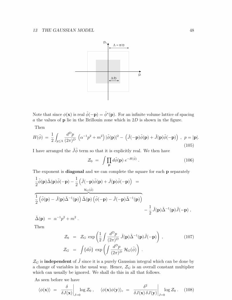
13 THE GAUSSIAN MODEL 48
Note that since φ(x) is real φ(−p) = φ∗(p). For an infinite volume lattice of spacinga the values of p lie in the Brillouin zone which in 2D is shown in the figure.
Then
H(φ) =1
2
∫p≤Λ
dDp
(2π)D
(α−1p2 +m2
)|φ(p)|2 −
(J(−p)φ(p) + J(p)φ(−p)
), p = |p|.
(105)I have arranged the J φ term so that it is explicitly real. We then have
Z0 =∫ ∏
p
dφ(p) e−H(φ) . (106)
The exponent is diagonal and we can complete the square for each p separately
1
2φ(p)∆(p)φ(−p)− 1
2
(J(−p)φ(p) + J(p)φ(−p)
)=
HG(φ)︷ ︸︸ ︷1
2
(φ(p)− J(p)∆−1(p)
)∆(p)
(φ(−p)− J(−p)∆−1(p)
)− 1
2J(p)∆−1(p)J(−p) ,
∆(p) = α−1p2 +m2 .
Then
Z0 = ZG exp
(1
2
∫ dDp
(2π)DJ(p)∆−1(p)J(−p)
), (107)
ZG =∫dφ exp
(∫ dDp
(2π)DHG(φ)
).
ZG is independent of J since it is a purely Gaussian integral which can be done bya change of variables in the usual way. Hence, ZG is an overall constant multiplierwhich can usually be ignored. We shall do this in all that follows.
As seen before we have
〈φ(x)〉 =δ
δJ(x)
∣∣∣∣∣J=0
logZ0 , 〈φ(x)φ(y)〉c =δ2
δJ(x) δJ(y)
∣∣∣∣∣J=0
logZ0 . (108)
13 THE GAUSSIAN MODEL 49
We also have
〈φ(q)φ(p)〉c =∫dx dy e−iq·xe−ip·y 〈φ(x)φ(y)〉c .
Using translation invariance 〈φ(x)φ(y)〉c = G0(r), r = y − x, and so, changingvariables to x and r,
〈φ(q)φ(p)〉c =∫dx dr e−i(q+p)·xe−ip·rG0(r) = (2π)Dδ(D)(p + q) G0(p) .
Thus〈φ(q)φ(p)〉c = (2π)Dδ(D)(p + q) G0(p) , (109)
but from (105) and (107) above
〈φ(q)φ(p)〉c = (2π)2D δ2
δJ(−q) δJ(−p)
∣∣∣∣∣J=0
logZ0 = (2π)Dδ(D)(p + q) ∆(p)−1
⇒ G0(p) = ∆−1(p) =α
p2 + αm2. (110)
[ It helps to note that
J(p) =∫dDq δ(p + q) J(−q) , ∆(p) = ∆(−p) . ]
We immediately have
G0(r) =∫ dDp
(2π)De−ip·x
α
p2 + αm2∼
ξe−r/ξ
(rξ)(D−1)/2a ξ r ,
1
r(D−2)a r ξ ,
with ξ−2 = αm2. Thus for α = 1 we have ξ = 1/m.
Also, from earlier, the susceptibility is given by the general result
χ =∫dx G(r) = G(0) ⇒
χ =1
m2= αξ2 . (111)
In an interacting theory we can block until Λ ξ = κ 1 and then, assuming, likeLG, that the interactions between the block spins are heavily suppressed, the theoryis well described by a Gaussian model with effective coupling constants α(Λ =κ ξ−1, T ),m(Λ = κ ξ−1, T ). From above we see that as ξ diverges at a critical pointso does χ. We might expect from this that since ξ ∼ |t|−ν and then χ ∼ |t|−2ν .However, we must allow that α(κ ξ−1, T ) ∼ ξρ ⇒ χ ∼ |t|−(2+ρ)ν instead. thishappens if fluctuations cannot be ignored, contrary to the LG idea. Then mustkeep interaction terms.
13 THE GAUSSIAN MODEL 50
To investigate such behaviour further we implement a RG transformation whichconsists of two steps: a thinning of high momentum degrees of freedom and a rescal-ing step, just as we did in earlier cases. We illustrate this procedure by applying tothe Gaussian model.
We set J(x) ≡ h, a constant. Then the relevant term in H is
h∫dx φ(x) = hφ(0) . (112)
1) Thinning. The blocking strategy is to divide φ into two parts:
φ(p) = φ<(p) + φ>(p)
φ<(p) =
φ(p) 0 ≤ p ≤ Λ/b0 Λ/b < p ≤ Λ
φ>(p) =
0 0 ≤ p ≤ Λ/b
φ(p) Λ/b < p ≤ Λ
This divides the Brillouin zone into two regions associated with low momentum andhigh momentum, respectively, using a scale factor b. We can then decompose thepartition function into a piece that depends on φ< only times a piece that dependson φ> only. This is easily done because the field theory is Gaussian. We get
Z0 =∫ ∏
p
dφ< e−H(φ<)
∫ ∏p
dφ> e−H(φ>) (113)
The integrals over φ> can be explicitly done since they are Gaussian and they simplygive an overall factor in the partition function which encodes their contribution tothe free energy. Only H(φ<) depends on h since h only couples to φ(0) ≡ φ<(0).
Z0 = e−βF>∫ ∏
p
dφ< exp(−H(φ<)
). (114)
The theory is described by H(φ<) but with a smaller cutoff Λ′ = Λ/b. In otherwords we have integrated out high momentum degrees of freedom and have a newor blocked theory defined on a Brillouin zone of extent given by Λ′.
The Hamiltonian of the blocked model is, in this case, the same as the original onebut with cut-off Λ′
H(φ<) =∫p<Λ′
dDp
(2π)D1
2
(α−1p2 +m2
)|φ<(p)|2 + hφ<(0) , p = |p|, (115)
(2) Rescaling. We rescale the momentum by a factor of b so that the Brillouin zone isrestored to its original size and hence the related cutoff to its original value. Thisis simply a change of units; in the blocking for the Ising model we always naturallyused the lattice spacing as our unit and this is just doing the same. However, We
13 THE GAUSSIAN MODEL 51
can also choose to rescale the field variable at the same time. We thus define therescalings
Λ′ → Λ = bΛ′ ,
p → q = bp ⇒ 0 ≤ q ≤ Λ ,
φ<(p) → φ(q) : φ<(p) = Z φ(q) . (116)
This is just a change of field integration variable. Note that the rescaling factor,Z, for the coordinate space field φ(x) is given by Z = b−DZ.
In terms of the new or blocked fields the blocked Hamiltonian is now
H =1
2Z2b−D
∫q≤Λ
dDq
(2π)D
(α−1 q
2
b2+m2
)|φ(q)|2 + Zhφ(0) . (117)
We can relabel q as p since it is a dummy integration variable. Then we see thatwe recover a Gaussian Hamiltonian of the same form as the original.
The important point is that the by thinning and then rescaling we have the samecutoff for the original and the blocked models. Of course, all quantities with dimen-sion will scale with b as well. For example, the correlation length for the blockedHamiltonian is smaller by a factor of b: ξ → ξ/b. The RG transformation denotedby R(b) is then
R(b) : H(φ, α,m, h,Λ) → H(φ, α′,m′, h′,Λ) ,
(α′)−1 = Z2 b−D−2α−1 ,
m′ = Z b−D/2m ,
h′ = Zh . (118)
This defines the RG equations for α−1,m, h. The question is what is most usefulchoice for the field rescaling factor Z? It should be emphasized that any choice forZ will yield correct results but there is a particular best choice. Some examples:
1) Z2 < bD. This choice implies that both α−1,m are irrelevant since they will flowto a fixed point at α−1 = m = 0. This is not very useful and must extract thephysics from the way these quantities decay to zero;
2) Z2 > bD+2. Both α−1,m are relevant near the f.p. at α−1 = m = 0. This isalso tricky to analyze although it is a choice that might be entertained for morecomplicated models.
In fact the best choice is Z2 = bD+2 for which we find the RG equations
(α′)−1 = α−1 , m′ = bm , h′ = bD/2+1h (119)
α is now constant and can be chosen as α = 1. Near to a critical point ξ = 1/mdiverges and we can expand m2 about T = Tc to give m2 ∼ |t|. We thus see from(119) that
|t| → |t′| = b2|t| ⇒ λt = 2 ,h → h′ = bD/2+1h ⇒ λh = D/2 + 1 .
(120)
14 THE PERTURBATION EXPANSION 52
This predicts
α = (4−D)/2 , β = (D − 2)/4 , ν = 1/2 , γ = 1 . (121)
These are not mean field predictions for α and β, but note that they do attain theirmean field values for D = 4. This is an indication that Dc = 4. At h = 0 from (88)
F±(u0, C0) = |t|D/λt (f± (0) + C±) + I±(t) . (122)
For D > 4 have D/λt = D/2 > 2 and the first term is less singular than the t2 termin I±(t) which therefore controls the specific heat exponent giving α = 0 which is themean field result. The way the critical behaviour becomes mean-field behaviour forthe other exponents is concerned with the idea of ”dangerous irrelevant variables”but will not discuss this here.
Note that this choice for Z corresponds to Z2 = b−D+2, where Z is the correspondingfield rescaling (or renormalization) factor for φ(x).
14 The Perturbation Expansion
We start with the definition
< φ(0)φ(z) >=1
Z
∫dφ φ(0)φ(z) e−S(φ) .
Let
S(φ) =∫dx
1
2(∇φ)2 +
1
2m2φ2 +
1
4!gφ4 ,
where m2 can be negative. The situation m2 < 0 corresponds to spontaneousbreaking of the symmetry φ→ −φ in the bare Hamiltonian. However, we shall seethat the effective mass is positive once loop corrections are included.
The quantities we need are the connected r-point functions
〈φ(z1)φ(z2) . . . φ(zr)〉c =δ
δJ(z1)
δ
δJ(z2). . .
δ
δJ(zr)
∣∣∣∣∣J=0
logZ(J) ,
whereZ(J) =
∫dφ e−S(φ)+Jφ , Jφ ≡
∫dx J(x)φ(x) .
We can calculate the expression for 〈〉c by example as we did before:
< φ(y)φ(z) >c = < φ(y)φ(z) > −〈φ(y)〉〈φ(z)〉 .
They are the physical response functions encoding the response to an external field.On physical grounds we would the expect that
〈φ(z1)φ(z2) . . . φ(zr)〉c → 0 |zi − zj| → ∞ like e−|zi−zj |/ξ .
This will not be true unless we subtract off all disconnected contributions. Note alsothat then ∫
dz1 . . . dzr 〈φ(z1)φ(z2) . . . φ(zr)〉c ∝ V , (123)
14 THE PERTURBATION EXPANSION 53
as is expected on physical grounds. For the moment we consider m2 > 0 and wehave
< φ(y)φ(z) >c =
(1
Zδ2
δJ(y)δJ(z)Z(J)
)−
(1
Zδ
δJ(y)Z(J)
) (1
Zδ
δJ(z)Z(J)
)∣∣∣∣∣J=0
.
However, the second term on RHS just subtracts off the disconnected piece, so ifwe restrict our calculation of the first term to connected contributions we can omitthese disconnected terms. We have
S(φ) =∫dx
1
2(∇φ)2 +
1
2m2φ2︸ ︷︷ ︸
S0
+∫dx
1
4!gφ4 ,
and so we consider
Z(J) =∫dφ e−S0(φ)+Jφ︸ ︷︷ ︸
Z0(J)
e−∫dx 1
4!gφ4
= e−g4!
∫dx ( δ
δJ(x))4
Z0(J) .
HereZ0(J) = e
12
∫dx dy J(x)G(x−y)J(y) .
Then (taking only connected contributions)
< φ(y)φ(z) >c =
δ2
δJ(y)δJ(z)e−
g4!
∫dx ( δ
δJ(x))4
Z0(J)
e−g4!
∫dx ( δ
δJ(x))4
Z0(J)
∣∣∣∣∣∣∣J=0
.
We tacitly cancel overall constant multipliers such as ZG discussed before. We nowexpand both numerator and denominator as a series in g. We note that the denomi-nator does not depend on y, z and so will only contribute disconnected terms whenthe whole expression is written as a power series in g. Because they are disconnectedthese contribute terms diverge with the volume V and must ultimately cancel oth-erwise (123) would not hold . In fact, this is ensured because the denominator is afactor of the numerator. Hence, we recover the terms we want by considering onlythe connected terms from the numerator. This will be understood from now on.
The O(g0) term is just what we calculated in the Gaussian model and so we find
< φ(y)φ(z) >c =δ2
δJ(y)δJ(z)Z0(J)
∣∣∣∣∣J=0
= G0(z− y) + O(g) .
The O(g) term is
− g4!
δ2
δJ(y)δJ(z)
∫dx
(δ
δJ(x)
)4
Z0(J)
∣∣∣∣∣∣J=0
.
The rules for differentiating Z0(J) are clear. Every pair of derivatives gives a Gaus-sian two-point function, or propagator, G0(r). Thus we can immediately write down
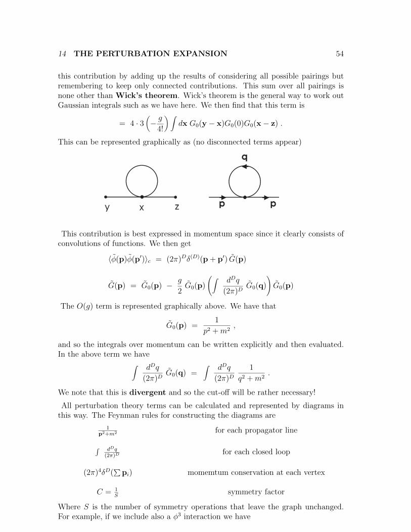
14 THE PERTURBATION EXPANSION 54
this contribution by adding up the results of considering all possible pairings butremembering to keep only connected contributions. This sum over all pairings isnone other than Wick’s theorem. Wick’s theorem is the general way to work outGaussian integrals such as we have here. We then find that this term is
= 4 · 3(− g
4!
) ∫dx G0(y − x)G0(0)G0(x− z) .
This can be represented graphically as (no disconnected terms appear)
This contribution is best expressed in momentum space since it clearly consists ofconvolutions of functions. We then get
〈φ(p)φ(p′)〉c = (2π)Dδ(D)(p + p′) G(p)
G(p) = G0(p) − g
2G0(p)
(∫ dDq
(2π)DG0(q)
)G0(p)
The O(g) term is represented graphically above. We have that
G0(p) =1
p2 +m2,
and so the integrals over momentum can be written explicitly and then evaluated.In the above term we have∫ dDq
(2π)DG0(q) =
∫ dDq
(2π)D1
q2 +m2.
We note that this is divergent and so the cut-off will be rather necessary!
All perturbation theory terms can be calculated and represented by diagrams inthis way. The Feynman rules for constructing the diagrams are
1p2+m2 for each propagator line
∫ dDq(2π)D
for each closed loop
(2π)4δD(∑
pi) momemtum conservation at each vertex
C = 1S
symmetry factor
Where S is the number of symmetry operations that leave the graph unchanged.For example, if we include also a φ3 interaction we have
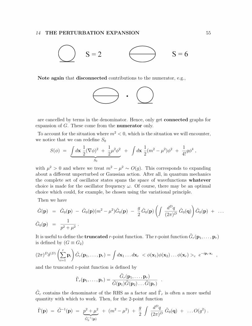
14 THE PERTURBATION EXPANSION 55
Note again that disconnected contributions to the numerator, e.g.,
are cancelled by terms in the denominator. Hence, only get connected graphs forexpansion of G. These come from the numerator only.
To account for the situation where m2 < 0, which is the situation we will encounter,we notice that we can redefine S0
S(φ) =∫dx
1
2(∇φ)2 +
1
2µ2φ2︸ ︷︷ ︸
S0
+∫dx
1
2(m2 − µ2)φ2 +
1
4!gφ4 ,
with µ2 > 0 and where we treat m2 − µ2 ∼ O(g). This corresponds to expandingabout a different unperturbed or Gaussian action. After all, in quantum mechanicsthe complete set of oscillator states spans the space of wavefunctions whateverchoice is made for the oscillator frequency ω. Of course, there may be an optimalchoice which could, for example, be chosen using the variational principle.
Then we have
G(p) = G0(p) − G0(p)(m2 − µ2)G0(p) − g
2G0(p)
(∫ dDq
(2π)DG0(q)
)G0(p) + . . .
G0(p) =1
p2 + µ2.
It is useful to define the truncated r-point function. The r-point function Gr(p1, . . . ,pr)is defined by (G ≡ G2)
(2π)Dδ(D)
(r∑i=1
pi
)Gr(p1, . . . ,pr) =
∫dx1 . . . dxr < φ(x1)φ(x2) . . . φ(xr) >c e−ipi·xi ,
and the truncated r-point function is defined by
Γr(p1, . . . ,pr) =Gr(p1, . . . ,pr)
G(p1)G(p2) . . . G(pr).
Gr contains the denominator of the RHS as a factor and Γr is often a more usefulquantity with which to work. Then, for the 2-point function
Γ(p) = G−1(p) = p2 + µ2︸ ︷︷ ︸G−1
0 (p)
+ (m2 − µ2) +g
2
∫ dDq
(2π)DG0(q) + . . . O(g2) .
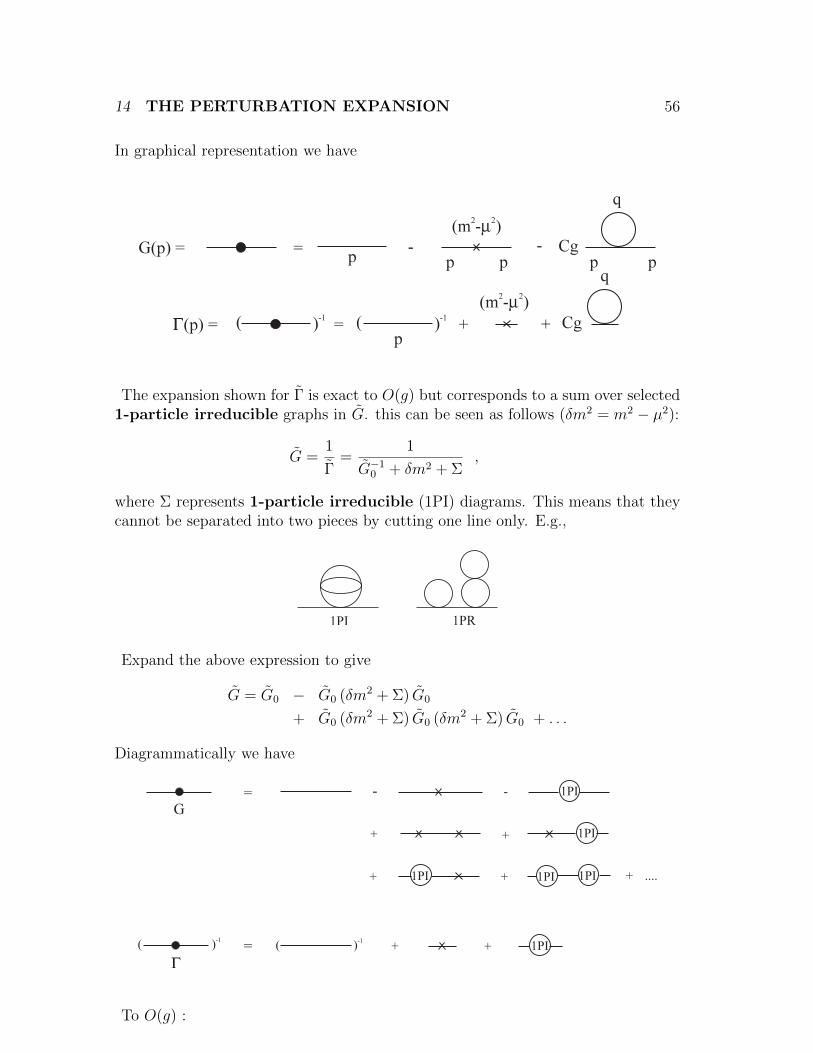
14 THE PERTURBATION EXPANSION 56
In graphical representation we have
The expansion shown for Γ is exact to O(g) but corresponds to a sum over selected1-particle irreducible graphs in G. this can be seen as follows (δm2 = m2 − µ2):
G =1
Γ=
1
G−10 + δm2 + Σ
,
where Σ represents 1-particle irreducible (1PI) diagrams. This means that theycannot be separated into two pieces by cutting one line only. E.g.,
Expand the above expression to give
G = G0 − G0 (δm2 + Σ) G0
+ G0 (δm2 + Σ) G0 (δm2 + Σ) G0 + . . .
Diagrammatically we have
To O(g) :
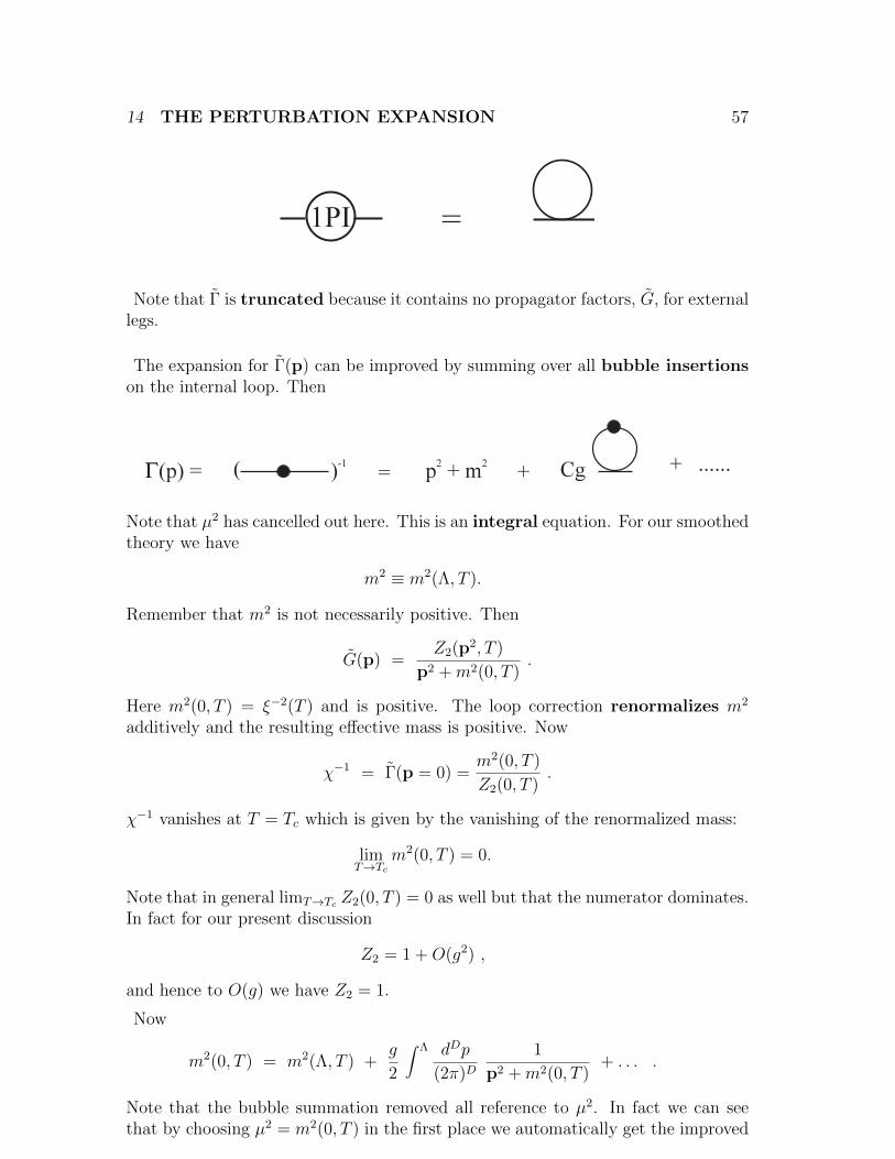
14 THE PERTURBATION EXPANSION 57
Note that Γ is truncated because it contains no propagator factors, G, for externallegs.
The expansion for Γ(p) can be improved by summing over all bubble insertionson the internal loop. Then
Note that µ2 has cancelled out here. This is an integral equation. For our smoothedtheory we have
m2 ≡ m2(Λ, T ).
Remember that m2 is not necessarily positive. Then
G(p) =Z2(p2, T )
p2 +m2(0, T ).
Here m2(0, T ) = ξ−2(T ) and is positive. The loop correction renormalizes m2
additively and the resulting effective mass is positive. Now
χ−1 = Γ(p = 0) =m2(0, T )
Z2(0, T ).
χ−1 vanishes at T = Tc which is given by the vanishing of the renormalized mass:
limT→Tc
m2(0, T ) = 0.
Note that in general limT→Tc Z2(0, T ) = 0 as well but that the numerator dominates.In fact for our present discussion
Z2 = 1 +O(g2) ,
and hence to O(g) we have Z2 = 1.
Now
m2(0, T ) = m2(Λ, T ) +g
2
∫ Λ dDp
(2π)D1
p2 +m2(0, T )+ . . . .
Note that the bubble summation removed all reference to µ2. In fact we can seethat by choosing µ2 = m2(0, T ) in the first place we automatically get the improved
14 THE PERTURBATION EXPANSION 58
formula from the one-loop expression. The coefficient of 12
comes from the symmetryfactor as described above. Using m2(0, Tc) = 0 we write
m2(0, T ) = m2(Λ, T ) − m2(Λ, Tc) +g
2
∫ Λ dDp
(2π)D
[1
p2 +m2(0, T )− 1
p2
]
= At− g
2m2(0, T )
∫ Λ dDp
(2π)D1
(p2 +m2(0, T ))p2+ . . .
Where t = (T − Tc)/Tc.We consider two cases:
D > 4 The integral is dominated by large p and is finite in the limit m2 → 0. Then
m2(0, T ) = At+Bm2(0, T ).
This is consistent with the Landau behaviour
m2(0, T ) = Ct
D < 4 The integral is sensitive to low p and is Infra-Red divergent unless m2 > 0:
m2(0, T ) = At+BmD−2(0, T )
This is clearly inconsistent with the Landau assumption: the integral is important.IR divergences invalidate Landau’s assumption.
D = 4 A marginal case with IR logarithmic corrections
m2(0, T ) = At+Bm2 logm2.
Get Landau behaviour modified by logs.
Hence Dc = 4 and for D ≤ 4 IR effects destroy mean-field predictions.
This theory applies to an ordinary critical point in Landau’s theory: the coefficientof φ2 vanishes. If, for some reason, the φ4 were absent and the interaction startedat the gφ6 term then the loop contribution would be
∼∫ Λ dDp
(2π)D1
p2 +m2(0, T )
∫ Λ dDq
(2π)D1
q2 +m2(0, T ).
Subtracting off the value at m2 = 0 and isolating the most IR divergent integralgives
∫ Λ dDp
(2π)D
∫ Λ dDq
(2π)D1
p2(p2 +m2(0, T ))(q2 +m2(0, T )).
15 THE GINSBERG CRITERION FOR DC 59
There are no IR problems for 2D− 6 > 0, i.e., D > 3. Hence in this case Dc = 3. InLandau’s theory this situation corresponds to a tricritical point: the coefficients ofφ2 and φ4 vanish.
In general, for interaction φ2n we find
(n− 1)Dc − 2n = 0,
or
Dc =2n
n− 1.
This interaction is relevant only for critical points of order n. For D = 2 allcritical points show anomalous behaviour but for D = 3 only critical and tricriticalpoints are anomalous, and even then the corrections to mean-field predictions at thetricritical point are only logarithmic.
15 The Ginsberg Criterion for Dc
Mean Field Theory breaks down because the assumption that we may ignore fluc-tuations as T → Tc, ξ → ∞ is wrong. The alternative way to say this is thatInfra-Red effects are important. This is true for sufficiently low dimensions D ≤ Dc,where Dc depends on the kind of transition being considered: Dc = 4 for a CriticalPoint and Dc = 3 for a TriCritical Point.
The susceptibity χ per unit volume is
χ ∼∫dDx G(x) ∼
∫dDx
e−r/ξ
rD−2∼ ξ2.
In LG theory we found that χ ∼ |t|−1 and so we deduce that ξ2 ∼ |t|−1 as well.I.e., for LG have [t] = 1/2.
The fluctuations are coherent, or correlated, over a block of linear size L ∼ ξ sothat V ∼ ξD. Measure everything now ”per block of size ξ”; this is the new “unitvolume”.
(1) Now looking at the block of size ∼ ξ, the fluctuation is of magnitude
∆M2 =∫dDxdDy 〈φ(x)φ(y)〉 − 〈φ(x)〉〈φ(y)〉 ≡ V
∫dDx G(x).
I.e., the susceptibility (up to factors). Thus, from above
∆M2 = V ξ2 ∼ ξD+2.
(2) In LG theory for some general continuous transition with T ≤ Tc the free energy is
A ∼ − a2|t|M2 + A2nM2n + . . . =⇒ M ∼ V |t|1/(2n−2)
Thus, we findM ∼ ξD−1/(n−1).
15 THE GINSBERG CRITERION FOR DC 60
Then for LG to work we need that the fluctuations become unimportant w.r.t. Mas t→ 0. Now,
∆M2
M2∼ ξ(D+2)
ξ2D−2/(n−1)
and we thus require
(D + 2)− 2D + 2/(n− 1) < 0 =⇒ D > Dc =2n
n− 1.
For n = 2 (CP) have Dc = 4, and for n = 3 (TCP) have Dc = 3.
Our anomalous scaling analysis works for D ≤ Dc where generally the fixed pointsare at non-zero values of the couplings. For D > Dc Mean Field Theory holds andfixed points are Gaussian in nature. The change over requires an analysis of so-called“dangerous irrelevant variables”.
16 CALCULATION OF THE CRITICAL INDEX 61
Notes and Extra Material
16 Calculation of the Critical Index
This section is concerned with the calculation of the critical index ν in the Isingmodel. We work with φ4 field theory in D dimensions.
S(φ) =∫dx
1
2(∇φ)2 +
1
2m2φ2 +
1
4!gφ4 + . . .[
m2]
= 2 [g] = 4−D ≡ ε .
We may imagine that we have obtained this action by integrating out the shortwavelength modes. In general all types of interaction are present. Clearly φ hasbeen renormalized to give the canonical form to the kinetic term. Alternatively, wecan accept that S(φ) has been generated from the Ising model by the transformationdescribed in earlier sections. We note for interest that the Ising model is identicalto φ4 field theory in the limit m2 → −∞, g →∞ such that 6|m2|/g = 1.
Suppose that we have integrated over all momenta p > Λ and that the effectiveparameters are m2(Λ, T ) and g(Λ, T ). We shall also allow for multiplicative fieldrenormalization constant Z(Λ, T ). Now integrate over the next momentum slice.Write
φ(x) = φ>(x) + φ<(x) .
φ> contains contributions from momenta in the range Λ− δΛ ≤ p < Λ.
φ< contains contributions from momenta in the range 0 ≤ p < Λ− δΛ.
Then
Z =∫dφ<dφ> e−S(φ>+φ<) .
We do the integrals over φ> to get an action as a function of φ< only.
S(φ< + φ>) = S(φ<) + S(φ>) +∫dx[∇φ>∇φ< +m2φ<φ>
]+
g
12
∫dx[2φ3
<φ> + 3φ2<φ
2> + 2φ<φ
3>
].
The term quadratic in the fields vanishes identically. Since in p-space φ> and φ<have disjoint support∫
dxφ>(x)φ<(x) =∫dpφ<(p)φ>(−p) = 0 .
Then
Z =∫dφ< e−S(φ<)
∫dφ> e−S(φ>) e−
g12
∫dx[2φ3<φ>+3φ2<φ
2>+2φ<φ3>] .
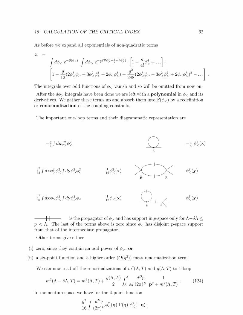
16 CALCULATION OF THE CRITICAL INDEX 62
As before we expand all exponentials of non-quadratic terms
Z = ∫dφ< e−S(φ<)
∫dφ> e−
12
(∇φ2>+ 12m2φ2>) ·
[1− g
4!φ4> + . . .
]·[
1− g
12(2φ3
<φ> + 3φ2<φ
2> + 2φ<φ
3>) +
g2
288(2φ3
<φ> + 3φ2<φ
2> + 2φ<φ
3>)2 − . . .
].
The integrals over odd functions of φ< vanish and so will be omitted from now on.
After the dφ> integrals have been done we are left with a polynomial in φ< and itsderivatives. We gather these terms up and absorb them into S(φ<) by a redefinitionor renormalization of the coupling constants.
The important one-loop terms and their diagrammatic representation are
−g4
∫dxφ2
>φ2< −1
4φ2<(x)
g2
32
∫dxφ2
>φ2<
∫dyφ2
>φ2<
116φ2<(x) φ2
<(y)
g2
36
∫dxφ>φ
3<
∫dyφ3
>φ<112φ<(x) φ3
<(y)
is the propagator of φ> and has support in p-space only for Λ−δΛ ≤p < Λ. The last of the terms above is zero since φ< has disjoint p-space supportfrom that of the intermediate propagator.
Other terms give either
(i) zero, since they contain an odd power of φ>, or
(ii) a six-point function and a higher order (O(g2)) mass renormalization term.
We can now read off the renormalizations of m2(Λ, T ) and g(Λ, T ) to 1-loop
m2(Λ− δΛ, T ) = m2(Λ, T ) +g(Λ, T )
2
∫ Λ
Λ−δΛ
dDp
(2π)D1
p2 +m2(Λ, T ). (124)
In momentum space we have for the 4-point function
g2
16
∫ dDq
(2π)Dφ2<(q) Γ(q) φ2
<(−q) ,
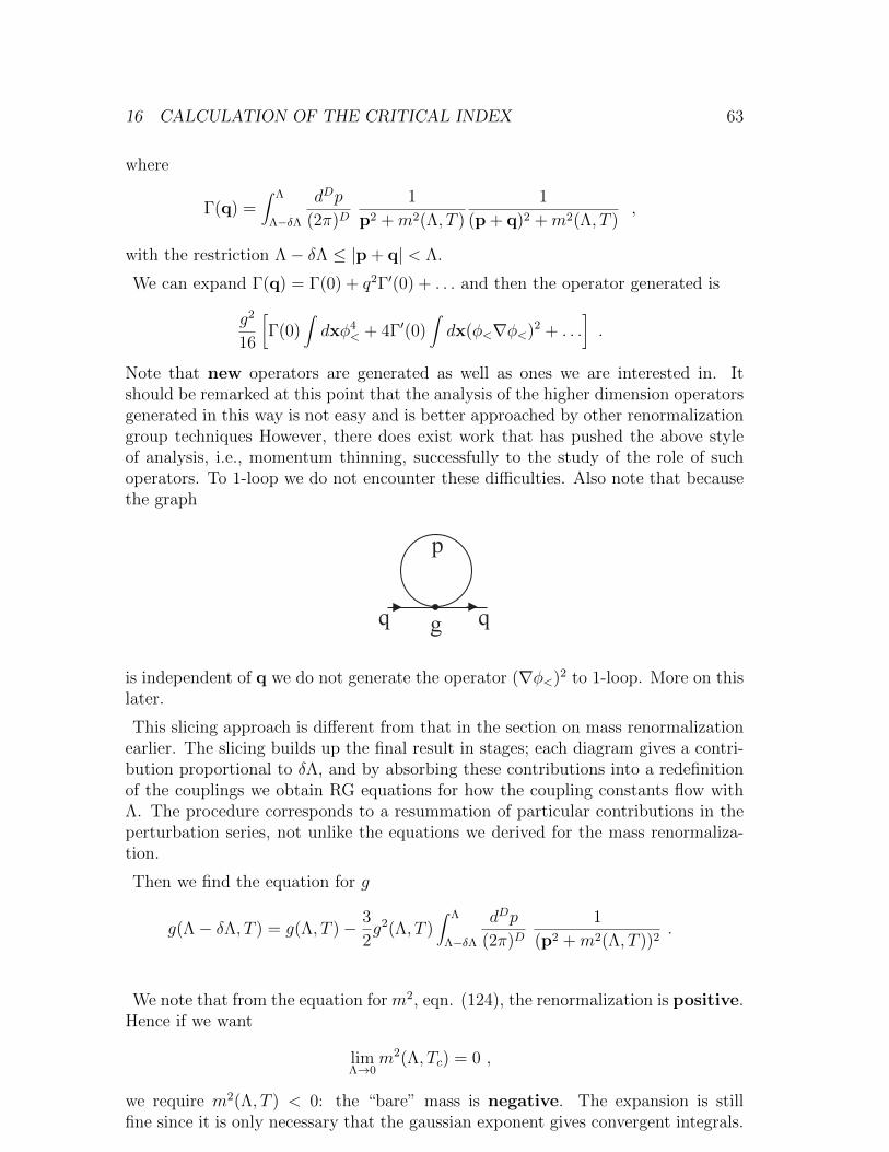
16 CALCULATION OF THE CRITICAL INDEX 63
where
Γ(q) =∫ Λ
Λ−δΛ
dDp
(2π)D1
p2 +m2(Λ, T )
1
(p + q)2 +m2(Λ, T ),
with the restriction Λ− δΛ ≤ |p + q| < Λ.
We can expand Γ(q) = Γ(0) + q2Γ′(0) + . . . and then the operator generated is
g2
16
[Γ(0)
∫dxφ4
< + 4Γ′(0)∫dx(φ<∇φ<)2 + . . .
].
Note that new operators are generated as well as ones we are interested in. Itshould be remarked at this point that the analysis of the higher dimension operatorsgenerated in this way is not easy and is better approached by other renormalizationgroup techniques However, there does exist work that has pushed the above styleof analysis, i.e., momentum thinning, successfully to the study of the role of suchoperators. To 1-loop we do not encounter these difficulties. Also note that becausethe graph
is independent of q we do not generate the operator (∇φ<)2 to 1-loop. More on thislater.
This slicing approach is different from that in the section on mass renormalizationearlier. The slicing builds up the final result in stages; each diagram gives a contri-bution proportional to δΛ, and by absorbing these contributions into a redefinitionof the couplings we obtain RG equations for how the coupling constants flow withΛ. The procedure corresponds to a resummation of particular contributions in theperturbation series, not unlike the equations we derived for the mass renormaliza-tion.
Then we find the equation for g
g(Λ− δΛ, T ) = g(Λ, T )− 3
2g2(Λ, T )
∫ Λ
Λ−δΛ
dDp
(2π)D1
(p2 +m2(Λ, T ))2.
We note that from the equation for m2, eqn. (124), the renormalization is positive.Hence if we want
limΛ→0
m2(Λ, Tc) = 0 ,
we require m2(Λ, T ) < 0: the “bare” mass is negative. The expansion is stillfine since it is only necessary that the gaussian exponent gives convergent integrals.
16 CALCULATION OF THE CRITICAL INDEX 64
Inspecting the denominator of the integrand in eqn. (124) this demands only thatthis denominator remains positive and so that
Λ2 > −m2(Λ, T ) ∀Λ .
It can be verified in what follows that this inequality is always respected.
We now rewrite the two renormalization equations in differential form in terms ofdimensionless quantities.
u2(b, T ) = Λ−2m2(Λ, T )
λ(b, T ) = Λ−εg(Λ, T ) ,
where b = log(Λ0/Λ) and ε = 4−D. Λ0 is the cut-off for the original theory.
Then we have the evolution equations
du2
db= 2u2 +
ΩD
2(2π)Dλ
1 + u2
dλ
db= ελ− 3ΩD
2(2π)Dλ2
(1 + u2)2, (125)
ΩD is the surface area of a unit sphere in D dimensions: Ω4 = 2π2.
In order to integrate these equations the propagator for φ< must take the canonicalform 1/(p2 +m2). In general, after integrating over the momentum shell of thicknessδΛ, the renormalized action, SR(φ<) will be of the form
SR(φ<) = S(φ<) +1
2δm2φ2
< +1
4!δgφ4
<
− 1
2δz(∇φ<)2 +
1
4!δg′(φ<∇φ<)2 + . . . ,
where δz determines the field rescaling or renormalization. We would like to keepthe coefficient of ∇φ<∇φ< to be unity at each step (just like in the Gaussian model)and so we can renormalize the field at each step so that this is true. This meanswe start the next step from the same style of action as the previous one and can soeasily iterate (i.e., integtate) the RG equations. This is a component of the scalingpart of the RG apprpoach which we describe now.
As in the Gaussian model, we can perform a rescaling so that we recover the samecut-off Λ0 but in new units. Note, that under this rescaling u and λ do not changesince they are dimensionless. We carry out the rescaling every time we integrate outa shell from Λ to Λ− δΛ. Of course, the value of b keeps track of the total amountof rescaling.
Let κ = eb. After integration of the RG equation above we can write the RGfollowed by the rescaling step as follows:
In momentum space we have
Λ0 → Λ → Λ0 = κΛ ,
p → p → q = κp ⇒ 0 ≤ q ≤ Λ0 ,
φ<(p) → φ<(p) → φ′(q) = Z−1 φ<(p) . (126)
16 CALCULATION OF THE CRITICAL INDEX 65
In coordinate space we have
a0 → a → a0 = a/κ ,
x → x → x0 = x/κ ,
φ<(x) → φ<(x) → φ′(x0) = Z−1 φ<(x) . (127)
Since φ(p) is the Fourier transform of φ(x) we find immediately that Z(b) = κD Z(b).This follows because the measures in the Fourier transforms for p and q are dDpand dDq, respectively, and dDq = κDdDp; it is just like in the Gaussian model.
From the definitions of u and λ we have, in either case,
u(b, T ) → uR(b, T ) = Z(b, T )u(b, T )
λ(b, T ) → λR(b, T ) = Z4(b, T )λ(b, T ) ,
and the RG equations above must be modified accordingly to give the flows for uRand λR.
However, we have note that to the order in which we are working,(1-loop), Z = 1.Henceforth, we set Z = 1 above, and identify (uR, λR) with (u, λ). In a general case,we would need to compute Z(b, T ) but in φ4 theory this is hard and needs somefurther work.
It is important to remark at this stage that the renormalization choices I am making(e.g. defining the coefficient of the kinetic term to be unity), are not forced on meby physics: they are convenient for the perturbative-style analysis. Other choicesmay be necessary in more complex situations in order to reveal the structure of morecomplex phase transitions in the most effective way.
The transformation takes the form
S(φ, u2, λn,Λ0)integration−→ S(Z−1φ, u2(b), λn(b), e−bΛ0)
rescaling−→ S(φ, u2R(b), λRn(b),Λ0) .
Here Z ≡ Z(b), u = m/Λ and λn is the dimensionless coupling derived from theactual coupling gn associated with field monomial of order n. This is the core of therenormalization group transformation with the RG flow equations given above in(125). Note that by dealing with dimensionless quantities all explicit referenceto the cut-off Λ disappears.
The fixed points (u∗2, λ∗) of these RG equations are
ε < 0 (0 , 0) trivial f.p. - IR attractive
ε > 0 (0 , 0) trivial f.p. - UV attractive
(− ε6
,16π2
3ε) non-trivial f.p. - IR attractive
In the neighbourhood of the non-trivial f.p. we have, to O(ε)(dx/dbdy/db
)=
(2− 1
3ε 1
3ε
0 −ε
)(xy
),
where x = u2 − u∗2, y = λ− λ∗. As before x ∝ t. then
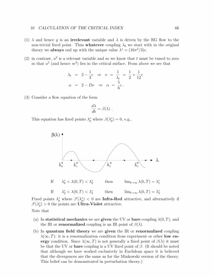
16 CALCULATION OF THE CRITICAL INDEX 66
(1) λ and hence g is an irrelevant variable and λ is driven by the RG flow to thenon-trivial fixed point. Thus whatever coupling λ0 we start with in the originaltheory we always end up with the unique value λ∗ = (16π2/3)ε.
(2) in contrast, u2 is a relevant variable and so we know that t must be tuned to zeroso that u2 (and hence m2) lies in the critical surface. From above we see that
λt = 2− 1
3ε ⇒ ν =
1
λt=
1
2+
1
12ε
α = 2−Dν ⇒ α =5
6ε .
(3) Consider a flow equation of the form
dλ
db= β(λ) .
This equation has fixed points λ∗p where β(λ∗p) = 0, e.g.,
If λ∗0 < λ(0, T ) < λ∗2 then limb→∞ λ(b, T ) = λ∗1
If λ∗2 < λ(0, T ) < λ∗4 then limb→∞ λ(b, T ) = λ∗3
Fixed points λ∗p where β′(λ∗p) < 0 are Infra-Red attractive, and alternatively ifβ′(λ∗p) > 0 the points are Ultra-Violet attractive.
Note that
(a) In statistical mechanics we are given the UV or bare coupling λ(0, T ), andthe IR or renormalized coupling is an IR point of β(λ).
(b) In quantum field theory we are given the IR or renormalized couplingλ(∞, T ): it is a renormalization condition from experiment or other low en-ergy condition. Since λ(∞, T ) is not generally a fixed point of β(λ) it mustbe that the UV or bare coupling is a UV fixed point of β. (It should be notedthat although we have worked exclusively in Euclidean space it is believedthat the divergences are the same as for the Minkowski version of the theory.This belief can be demonstrated in perturbation theory.)
16 CALCULATION OF THE CRITICAL INDEX 67
In our calculation we found the fixed points (u∗2, λ∗)
ε < 0 (0 , 0) trivial f.p. - IR attractive
ε > 0 (0 , 0) trivial f.p. - UV attractive
(− ε6
,16π2
3ε) non-trivial f.p. - IR attractive
It is believed that there are no others, not even at λ =∞. This means for quantumfield theory that there is no UV fixed point to be associated with the bare couplingexcept the one at (0, 0) when ε < 0. Hence, it follow that
ε < 0 λR = 0
ε ≥ 0 λR ≤ 16π2
3ε,
where λR = λ(b = ∞, T ). This is the statement of triviality for φ4 quantum fieldtheory. It means that in dimension four or greater the only consistent renormalizedφ4 theory in the limit of infinite cut-off is a free theory: λR = 0. Of course, weare not required to take the cut-off to infinity, rather we should keep it much largerthan the physical momentum scales on which the theory is being applied. Eventhen, for finite Λ the analysis presented gives an upper limit to λR. Such upperlimits have been used to set upper bounds on the Higgs mass in the most commonversion of the standard model.
Since ε is small we can get a reliable expansion in ε for both u∗2 and λ∗. This isthe epsilon expansion
λ∗ =∞∑n=1
anεn .
It is hoped that the radius of convergence is greater than one, thus including resultsfor D = 3.
(4) In the Landau theory we associate the coefficient of M4 with the low-momentumdimensionful coupling
g(T ) = Λε0 limb→∞
e−εbλ(b, T ) .
This is because g(T ) is the coefficient of M4 in the effective action derived by theLegendre transform. (Z = 1 to O(ε) otherwise we would need to include Z2 in thedefinition of g(T )).
Let
g(b, T ) = e−εbλ(b, T ) .
Then the equation for the flow of λ in the neighbourhood of the fixed point implies
dg
db= − 3
16π2eεbg2 ,
17 GENERAL IDEAS 68
or
1
g(b)− 1
g(b)= − 3
16π2eεb(eε(b−b) − 1
),
and thus
g(b) =g(b)
1 + a(ε)ε
(eε(b−b) − 1
) .a(ε) =
3
16π2eεb .
Denoting g(T ) ≡ g(∞, T ) we have the following results
ε > 0 : g(T ) = 0. Hence Landau’s method fails and the relevant physics is encodedin how g(b, T )→ 0 as b→∞.
ε < 0 : We have
g(T ) =g(b)
1 + a(ε)|ε|
.
Since here g(T ) is finite and non-zero Landau’s method works. As before weare assuming that b is large enough so that the equations we integrated to getthis result are valid. In this case g(T ) is actually independent of b.
ε = 0 : g(T ) = 0. Landau theory fails but
g(b) =g(b)
1 + 316π2 (b− b)
g(b) =g(b)
1 + 316π2 log Λ
Λ
.
I.e., only logarithmic violations of Landau theory.
17 General Ideas
Note. The general ideas of relating physical phenomena on widely differing scalesby renormalization group methods is widely applicable in many fields. For example:
(i) general diffusion models such as diffusion on fractal structures and the large scaleeffects of diffusive transport processes in fluid flow;
(ii) turbulence in fluids. The fluid velocity field, u(x, t), of fully developed turbulencehas energy density, as a function of wavenumber k,
k−2E(k) ∼ 1
V
∫dxdyu(x, t) · u(y, t)eik·(x−y)
with E(k) ∼ k−53 for large k.
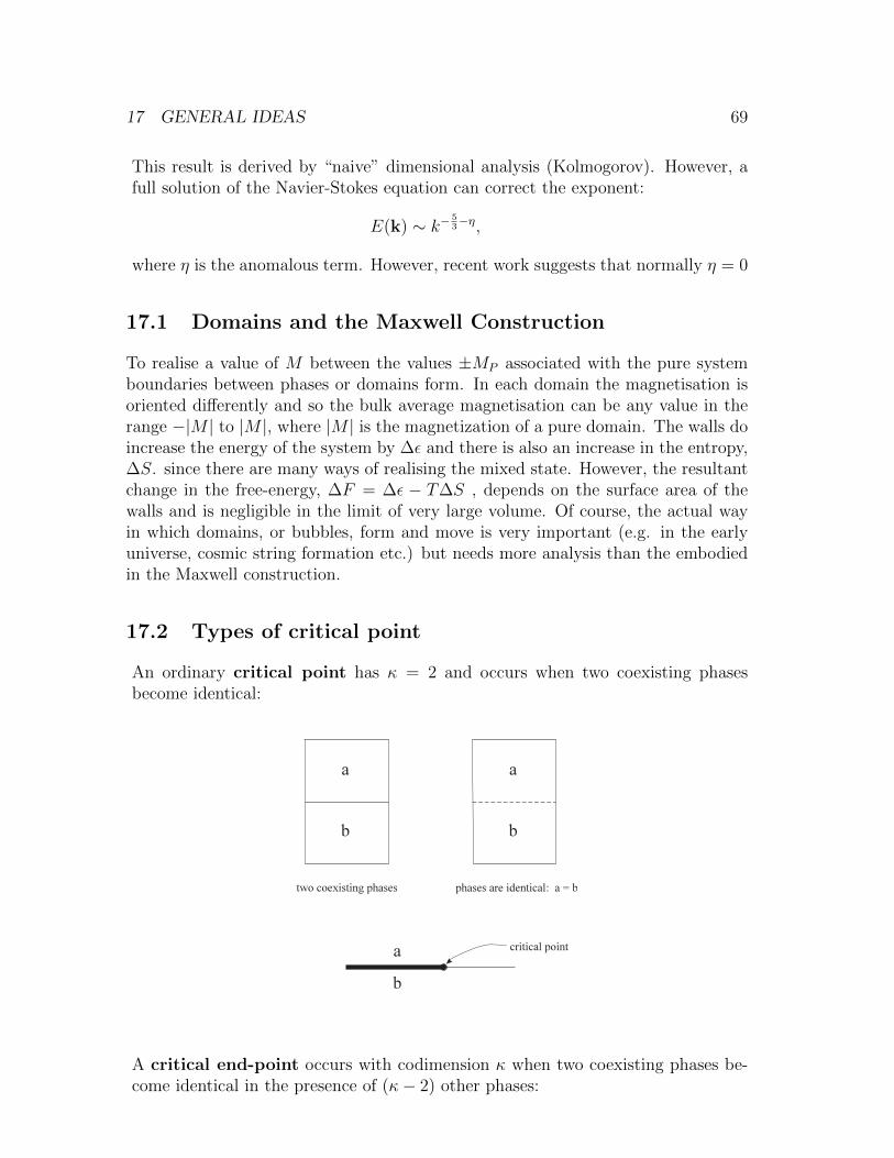
17 GENERAL IDEAS 69
This result is derived by “naive” dimensional analysis (Kolmogorov). However, afull solution of the Navier-Stokes equation can correct the exponent:
E(k) ∼ k−53−η,
where η is the anomalous term. However, recent work suggests that normally η = 0
17.1 Domains and the Maxwell Construction
To realise a value of M between the values ±MP associated with the pure systemboundaries between phases or domains form. In each domain the magnetisation isoriented differently and so the bulk average magnetisation can be any value in therange −|M | to |M |, where |M | is the magnetization of a pure domain. The walls doincrease the energy of the system by ∆ε and there is also an increase in the entropy,∆S. since there are many ways of realising the mixed state. However, the resultantchange in the free-energy, ∆F = ∆ε − T∆S , depends on the surface area of thewalls and is negligible in the limit of very large volume. Of course, the actual wayin which domains, or bubbles, form and move is very important (e.g. in the earlyuniverse, cosmic string formation etc.) but needs more analysis than the embodiedin the Maxwell construction.
17.2 Types of critical point
An ordinary critical point has κ = 2 and occurs when two coexisting phasesbecome identical:
A critical end-point occurs with codimension κ when two coexisting phases be-come identical in the presence of (κ− 2) other phases:
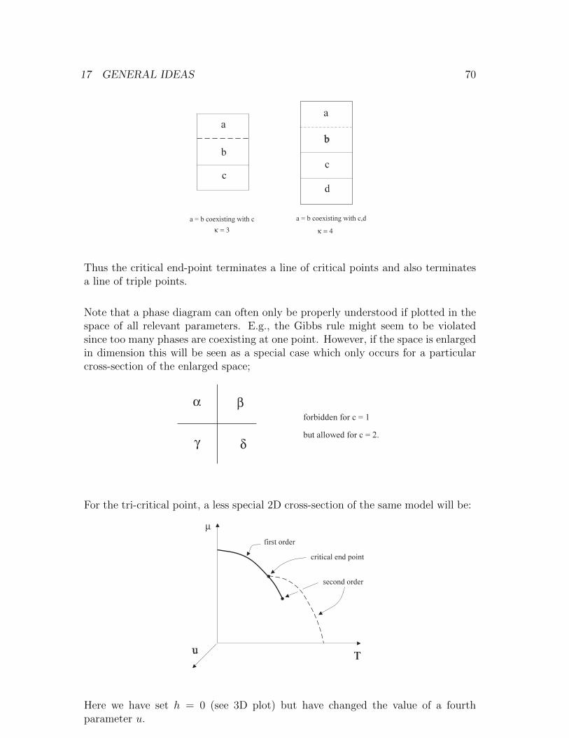
17 GENERAL IDEAS 70
Thus the critical end-point terminates a line of critical points and also terminatesa line of triple points.
Note that a phase diagram can often only be properly understood if plotted in thespace of all relevant parameters. E.g., the Gibbs rule might seem to be violatedsince too many phases are coexisting at one point. However, if the space is enlargedin dimension this will be seen as a special case which only occurs for a particularcross-section of the enlarged space;
For the tri-critical point, a less special 2D cross-section of the same model will be:
Here we have set h = 0 (see 3D plot) but have changed the value of a fourthparameter u.
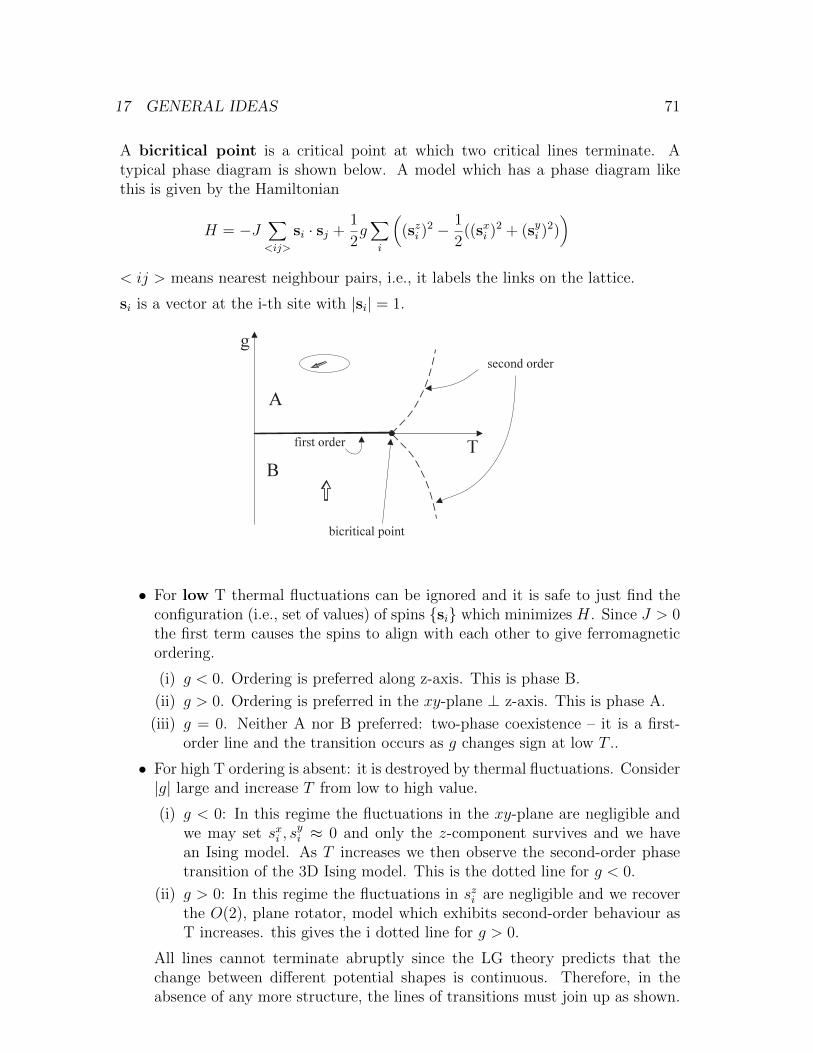
17 GENERAL IDEAS 71
A bicritical point is a critical point at which two critical lines terminate. Atypical phase diagram is shown below. A model which has a phase diagram likethis is given by the Hamiltonian
H = −J∑<ij>
si · sj +1
2g∑i
((szi )
2 − 1
2((sxi )
2 + (syi )2))
< ij > means nearest neighbour pairs, i.e., it labels the links on the lattice.
si is a vector at the i-th site with |si| = 1.
• For low T thermal fluctuations can be ignored and it is safe to just find theconfiguration (i.e., set of values) of spins si which minimizes H. Since J > 0the first term causes the spins to align with each other to give ferromagneticordering.
(i) g < 0. Ordering is preferred along z-axis. This is phase B.
(ii) g > 0. Ordering is preferred in the xy-plane ⊥ z-axis. This is phase A.
(iii) g = 0. Neither A nor B preferred: two-phase coexistence – it is a first-order line and the transition occurs as g changes sign at low T ..
• For high T ordering is absent: it is destroyed by thermal fluctuations. Consider|g| large and increase T from low to high value.
(i) g < 0: In this regime the fluctuations in the xy-plane are negligible andwe may set sxi , s
yi ≈ 0 and only the z-component survives and we have
an Ising model. As T increases we then observe the second-order phasetransition of the 3D Ising model. This is the dotted line for g < 0.
(ii) g > 0: In this regime the fluctuations in szi are negligible and we recoverthe O(2), plane rotator, model which exhibits second-order behaviour asT increases. this gives the i dotted line for g > 0.
All lines cannot terminate abruptly since the LG theory predicts that thechange between different potential shapes is continuous. Therefore, in theabsence of any more structure, the lines of transitions must join up as shown.
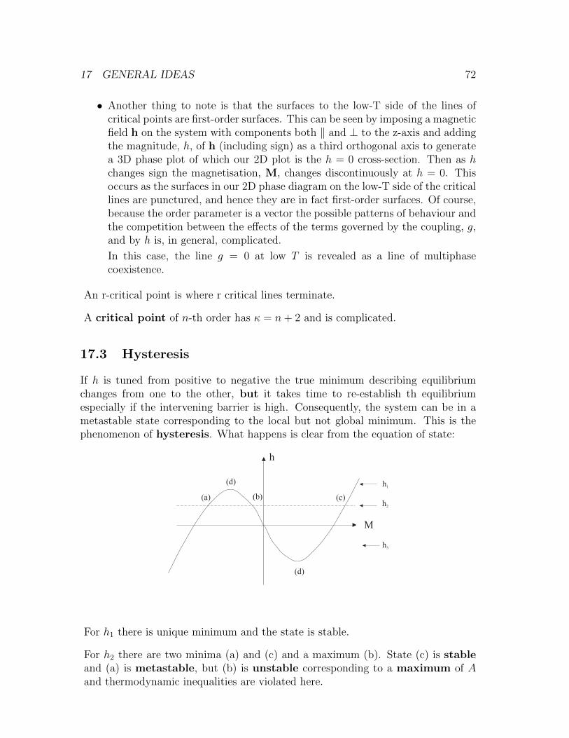
17 GENERAL IDEAS 72
• Another thing to note is that the surfaces to the low-T side of the lines ofcritical points are first-order surfaces. This can be seen by imposing a magneticfield h on the system with components both ‖ and ⊥ to the z-axis and addingthe magnitude, h, of h (including sign) as a third orthogonal axis to generatea 3D phase plot of which our 2D plot is the h = 0 cross-section. Then as hchanges sign the magnetisation, M, changes discontinuously at h = 0. Thisoccurs as the surfaces in our 2D phase diagram on the low-T side of the criticallines are punctured, and hence they are in fact first-order surfaces. Of course,because the order parameter is a vector the possible patterns of behaviour andthe competition between the effects of the terms governed by the coupling, g,and by h is, in general, complicated.
In this case, the line g = 0 at low T is revealed as a line of multiphasecoexistence.
An r-critical point is where r critical lines terminate.
A critical point of n-th order has κ = n+ 2 and is complicated.
17.3 Hysteresis
If h is tuned from positive to negative the true minimum describing equilibriumchanges from one to the other, but it takes time to re-establish th equilibriumespecially if the intervening barrier is high. Consequently, the system can be in ametastable state corresponding to the local but not global minimum. This is thephenomenon of hysteresis. What happens is clear from the equation of state:
For h1 there is unique minimum and the state is stable.
For h2 there are two minima (a) and (c) and a maximum (b). State (c) is stableand (a) is metastable, but (b) is unstable corresponding to a maximum of Aand thermodynamic inequalities are violated here.
17 GENERAL IDEAS 73
17.4 Mean Field Theory
The mean field approach is a type of variational principle. It can be formulated ina way due to Feynman and Peierls using the result that if g(x) is a convex functionthen 〈g(x)〉 ≥ g(〈x〉) whatever the probability distribution defining 〈.〉 (See Binneyet al). In particular, the exponential function is convex. Let H be the Hamiltonianof a model of interest and H0 the Hamiltonian of a related soluble model. Then wecan write
e−H = e−H0e−(H−H0)
⇒
e−F =∑σ
e−H = e−F0∑σ
e−H0
e−F0︸ ︷︷ ︸p0(σ)
e−(H−H0)
⇒e−F = e−F0 〈 e−(H−H0) 〉 ≥ e−F0 e−〈 H−H0 〉0
⇒F ≤ F0 + 〈 H −H0 〉0 , (128)
where 〈〉0 signifies averaging over the soluble model described by H0. In general,H0 will depend on a set of variational parameters, for example, the mean fieldmagnetization M . The best estimate for F is then to minimize the RHS of (128)w.r.t these parameters. Applied to the Ising model we recover the same results asabove. However, this formulation of the variational principle is very general and isused widely.
(2) For the Gaussian, or free, field theory in D > 1 we have ζ = [σ] = −(D − 2)/2since the kinetic term in the Hamiltonian
1
2
∫dDx (∇σ(x))2 , (129)
is dimensionless up to energy units. For r ξ there is no other dimensionful lengthbut r and so we have (see Eq. 73)
G(b−1r) = G(r′) = 〈σr′ σ0〉 = b−2ζ〈σr σ0〉 = b−2ζG(r)
⇒ G(r) ∼ 1
r−2ζ=
1
rD−2.