Preprint typeset in JHEP style - HYPER VERSION Lent Term, 2017

Solid State PhysicsUniversity of Cambridge Part II Mathematical Tripos

David Tong

Department of Applied Mathematics and Theoretical Physics,

Centre for Mathematical Sciences,

Wilberforce Road,

Cambridge, CB3 OBA, UK

http://www.damtp.cam.ac.uk/user/tong/solidstate.html

d.tong@damtp.cam.ac.uk

– 1 –

Recommended Books and Resources

There are many excellent books on Solid State Physics. The two canonical books are

• Ashcroft and Mermin, Solid State Physics

• Kittel, Introduction to Solid State Physics

Both of these go substantially beyond the material covered in this course. Personally,

I have a slight preference for the verbosity of Ashcroft and Mermin.

A somewhat friendlier, easier going book is

• Steve Simon, Solid State Physics Basics

It covers only the basics, but does so very well. (An earlier draft can be downloaded

from Steve Simon’s homepage; see below for a link.)

A number of lecture notes are available on the web. Links can be found on the course

webpage: http://www.damtp.cam.ac.uk/user/tong/solidstate.html

Contents

0. Introduction 1

1. Particles in a Magnetic Field 2

1.1 Gauge Fields 2

1.1.1 The Hamiltonian 3

1.1.2 Gauge Transformations 4

1.2 Landau Levels 5

1.2.1 Degeneracy 7

1.2.2 Symmetric Gauge 9

1.2.3 An Invitation to the Quantum Hall Effect 10

1.3 The Aharonov-Bohm Effect 13

1.3.1 Particles Moving around a Flux Tube 13

1.3.2 Aharonov-Bohm Scattering 15

1.4 Magnetic Monopoles 16

1.4.1 Dirac Quantisation 16

1.4.2 A Patchwork of Gauge Fields 19

1.4.3 Monopoles and Angular Momentum 20

1.5 Spin in a Magnetic Field 22

1.5.1 Spin Precession 24

1.5.2 A First Look at the Zeeman Effect 25

2. Band Structure 26

2.1 Electrons Moving in One Dimension 26

2.1.1 The Tight-Binding Model 26

2.1.2 Nearly Free Electrons 32

2.1.3 The Floquet Matrix 39

2.1.4 Bloch’s Theorem in One Dimension 41

2.2 Lattices 46

2.2.1 Bravais Lattices 46

2.2.2 The Reciprical Lattice 52

2.2.3 The Brillouin Zone 55

2.3 Band Structure 57

2.3.1 Bloch’s Theorem 58

2.3.2 Nearly Free Electrons in Three Dimensions 60

– 1 –

2.3.3 Wannier Functions 64

2.3.4 Tight-Binding in Three Dimensions 65

2.3.5 Deriving the Tight-Binding Model 66

2.4 Scattering Off a Lattice 72

2.4.1 The Bragg Condition 75

2.4.2 The Structure Factor 76

2.4.3 The Debye-Waller Factor 78

3. Electron Dynamics in Solids 80

3.1 Fermi Surfaces 80

3.1.1 Metals vs Insulators 81

3.1.2 The Discovery of Band Structure 86

3.1.3 Graphene 87

3.2 Dynamics of Bloch Electrons 91

3.2.1 Velocity 92

3.2.2 The Effective Mass 94

3.2.3 Semi-Classical Equation of Motion 95

3.2.4 Holes 97

3.2.5 Drude Model Again 99

3.3 Bloch Electrons in a Magnetic Field 101

3.3.1 Semi-Classical Motion 101

3.3.2 Cyclotron Frequency 103

3.3.3 Onsager-Bohr-Sommerfeld Quantisation 104

3.3.4 Quantum Oscillations 106

4. Phonons 109

4.1 Lattices in One Dimension 109

4.1.1 A Monotonic Chain 109

4.1.2 A Diatomic Chain 111

4.1.3 Peierls Transition 113

4.1.4 Quantum Vibrations 116

4.1.5 The Mossbauer Effect 120

4.2 From Atoms to Fields 123

4.2.1 Phonons in Three Dimensions 123

4.2.2 From Fields to Phonons 125

– 2 –

Acknowledgements

This material is taught as part of the “Applications in Quantum Mechanics” course of

the Cambridge mathematical tripos.

– 3 –

0. Introduction

Solid state physics is the study of “stuff”, of how the wonderfully diverse properties of

solids can emerge from the simple laws that govern electrons and atoms.

There is one, over-riding, practical reason for wanting to understand the behaviour

of stuff: this is how we build things. In particular, it is how we build the delicate

and powerful technologies that underlie our society. Important though they are, such

practicalities will take a back seat in our story. Instead, our mantra is “knowledge

for its own sake”. Indeed, the subject of solid state physics turns out to be one of

extraordinary subtlety and beauty. If such knowledge ultimately proves useful, this is

merely a happy corollary.

We will develop only the basics of solid state physics. We will learn how electrons

glide through seemingly impenetrable solids, how their collective motion is described by

a Fermi surface, and how the vibrations of the underlying atoms get tied into bundles

of energy known as phonons. We will learn that electrons in magnetic fields can do

strange things and start to explore some of the roles that geometry and topology play

in quantum physics.

One of the ultimate surprises of solid state physics is how the subject later dovetails

with ideas from particle physics. At first glance, one might have thought these two

disciplines should have nothing to do with each other. Yet one of the most striking

themes in modern physics is how ideas from one have influenced the other. In large

part this is because both subjects rest on some of the deepest principles in physics:

ideas such symmetry, topology and universality. Although much of what we cover in

these lectures will be at a basic level, we will nonetheless see some hints of these deeper

connections. We will, for example, see the Dirac equation — originally introduced to

unify relativity and quantum mechanics — emerging from graphene. We will learn how

the vibrations of a lattice, and the resulting phonons, provide a baby introduction to

quantum field theory.

– 1 –

1. Particles in a Magnetic Field

The purpose of this chapter is to understand how quantum particles react to magnetic

fields. In contrast to later sections, we will not yet place these particles inside solids,

for the simple reason that there is plenty of interesting behaviour to discover before we

do this. Later, in Section 3.1, we will understand how these magnetic fields affect the

electrons in solids.

Before we get to describe quantum effects, we first need to highlight a few of the

more subtle aspects that arise when discussing classical physics in the presence of a

magnetic field.

1.1 Gauge Fields

Recall from our lectures on Electromagnetism that the electric field E(x, t) and mag-

netic field B(x, t) can be written in terms a scalar potential φ(x, t) and a vector potential

A(x, t),

E = −∇φ− ∂A

∂tand B = ∇×A (1.1)

Both φ and A are referred to as gauge fields. When we first learn electromagnetism, they

are introduced merely as handy tricks to help solve the Maxwell equations. However,

as we proceed through theoretical physics, we learn that they play a more fundamental

role. In particular, they are necessary if we want to discuss a Lagrangian or Hamiltonian

approach to electromagnetism. We will soon see that these gauge fields are quite

indispensable in quantum mechanics.

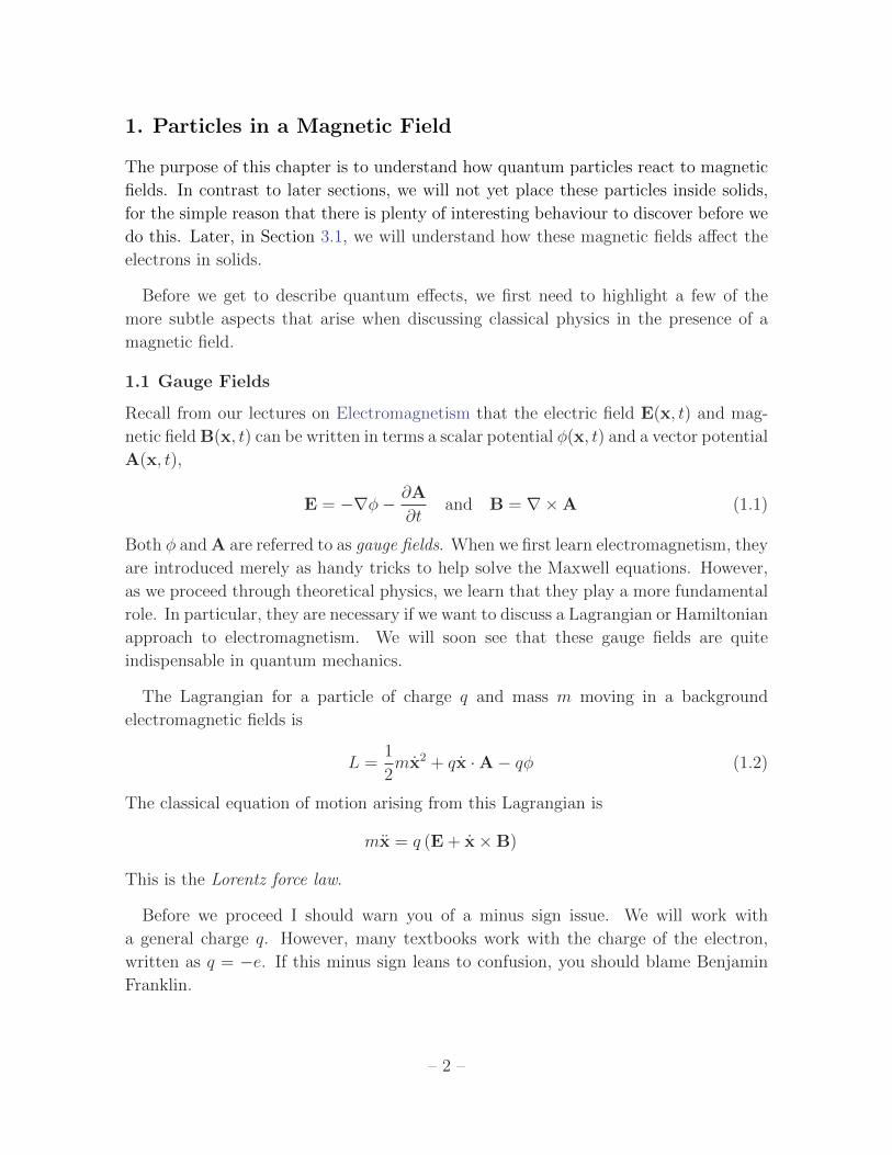
The Lagrangian for a particle of charge q and mass m moving in a background

electromagnetic fields is

L =1

2mx2 + qx ·A− qφ (1.2)

The classical equation of motion arising from this Lagrangian is

mx = q (E + x×B)

This is the Lorentz force law.

Before we proceed I should warn you of a minus sign issue. We will work with

a general charge q. However, many textbooks work with the charge of the electron,

written as q = −e. If this minus sign leans to confusion, you should blame Benjamin

Franklin.

– 2 –

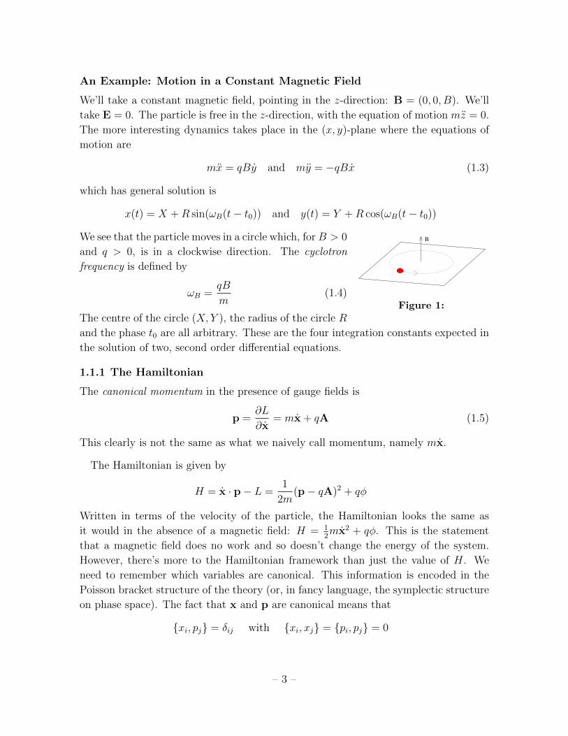
An Example: Motion in a Constant Magnetic Field

We’ll take a constant magnetic field, pointing in the z-direction: B = (0, 0, B). We’ll

take E = 0. The particle is free in the z-direction, with the equation of motion mz = 0.

The more interesting dynamics takes place in the (x, y)-plane where the equations of

motion are

mx = qBy and my = −qBx (1.3)

which has general solution is

x(t) = X +R sin(ωB(t− t0)) and y(t) = Y +R cos(ωB(t− t0))

We see that the particle moves in a circle which, forB > 0 B

Figure 1:

and q > 0, is in a clockwise direction. The cyclotron

frequency is defined by

ωB =qB

m(1.4)

The centre of the circle (X, Y ), the radius of the circle R

and the phase t0 are all arbitrary. These are the four integration constants expected in

the solution of two, second order differential equations.

1.1.1 The Hamiltonian

The canonical momentum in the presence of gauge fields is

p =∂L

∂x= mx + qA (1.5)

This clearly is not the same as what we naively call momentum, namely mx.

The Hamiltonian is given by

H = x · p− L =1

2m(p− qA)2 + qφ

Written in terms of the velocity of the particle, the Hamiltonian looks the same as

it would in the absence of a magnetic field: H = 12mx2 + qφ. This is the statement

that a magnetic field does no work and so doesn’t change the energy of the system.

However, there’s more to the Hamiltonian framework than just the value of H. We

need to remember which variables are canonical. This information is encoded in the

Poisson bracket structure of the theory (or, in fancy language, the symplectic structure

on phase space). The fact that x and p are canonical means that

xi, pj = δij with xi, xj = pi, pj = 0

– 3 –

In the quantum theory, this structure transferred onto commutation relations between

operators, which become

[xi, pj] = i~δij with [xi, xj] = [pi, pj] = 0

1.1.2 Gauge Transformations

The gauge fields A and φ are not unique. We can change them as

φ→ φ− ∂α

∂tand A→ A +∇α (1.6)

for any function α(x, t). Under these transformations, the electric and magnetic fields

(1.1) remain unchanged. The Lagrangian (1.2) changes by a total derivative, but this is

sufficient to ensure that the resulting equations of motion (1.3) are unchanged. Different

choices of α are said to be different choices of gauge. We’ll see some examples below.

The existence of gauge transformations is a redundancy in our description of the

system: fields which differ by the transformation (1.6) describe physically identical

configurations. Nothing that we can physically measure can depend on our choice of

gauge. This, it turns out, is a beautifully subtle and powerful restriction. We will start

to explore some of these subtleties in Sections 1.3 and 1.4

The canonical momentum p defined in (1.5) is not gauge invariant: it transforms

as p → p + q∇α. This means that the numerical value of p can’t have any physical

meaning since it depends on our choice of gauge. In contrast, the velocity of the particle

x is gauge invariant, and therefore physical.

The Schrodinger Equation

Finally, we can turn to the quantum theory. We’ll look at the spectrum in the next

section, but first we wish to understand how gauge transformations work. Following

the usual quantisation procedure, we replace the canonical momentum with

p 7→ −i~∇

The time-dependent Schrodinger equation for a particle in an electric and magnetic

field then takes the form

i~∂ψ

∂t= Hψ =

1

2m

(−i~∇− qA

)2

ψ + qφψ (1.7)

The shift of the kinetic term to incorporate the vector potential A is sometimes referred

to as minimal coupling.

– 4 –

Before we solve for the spectrum, there are two lessons to take away. The first is that

it is not possible to formulate the quantum mechanics of particles moving in electric

and magnetic fields in terms of E and B alone. We’re obliged to introduce the gauge

fields A and φ. This might make you wonder if, perhaps, there is more to A and φ

than we first thought. We’ll see the answer to this question in Section 1.3. (Spoiler:

the answer is yes.)

The second lesson follows from looking at how (1.7) fares under gauge transforma-

tions. It is simple to check that the Schrodinger equation transforms covariantly (i.e.

in a nice way) only if the wavefunction itself also transforms with a position-dependent

phase

ψ(x, t)→ eiqα(x,t)/~ψ(x, t) (1.8)

This is closely related to the fact that p is not gauge invariant in the presence of a mag-

netic field. Importantly, this gauge transformation does not affect physical probabilities

which are given by |ψ|2.

The simplest way to see that the Schrodinger equation transforms nicely under the

gauge transformation (1.8) is to define the covariant derivatives

Dt =∂

∂t+iq

~φ and Di =

∂

∂xi− iq

~Ai

In terms of these covariant derivatives, the Schrodinger equation becomes

i~Dtψ = − ~2mD2ψ (1.9)

But these covariant derivatives are designed to transform nicely under a gauge trans-

formation (1.6) and (1.8). You can check that they pick up only a phase

Dtψ → eiqα/~Dtψ and Diψ → eiqα/~Diψ

This ensures that the Schrodinger equation (1.9) transforms covariantly.

1.2 Landau Levels

Our task now is to solve for the spectrum and wavefunctions of the Schrodinger equa-

tion. We are interested in the situation with vanishing electric field, E = 0, and

constant magnetic field. The quantum Hamiltonian is

H =1

2m(p− qA)2 (1.10)

– 5 –

We take the magnetic field to lie in the z-direction, so that B = (0, 0, B). To proceed,

we need to find a gauge potential A which obeys ∇×A = B. There is, of course, no

unique choice. Here we pick

A = (0, xB, 0) (1.11)

This is called Landau gauge. Note that the magnetic field B = (0, 0, B) is invariant

under both translational symmetry and rotational symmetry in the (x, y)-plane. How-

ever, the choice of A is not; it breaks translational symmetry in the x direction (but not

in the y direction) and rotational symmetry. This means that, while the physics will

be invariant under all symmetries, the intermediate calculations will not be manifestly

invariant. This kind of compromise is typical when dealing with magnetic field.

The Hamiltonian (1.10) becomes

H =1

2m

(p2x + (py − qBx)2 + p2

z

)Because we have manifest translational invariance in the y and z directions, we have

[py, H] = [pz, H] = 0 and can look for energy eigenstates which are also eigenstates of

py and pz. This motivates the ansatz

ψ(x) = eikyy+ikzz χ(x) (1.12)

Acting on this wavefunction with the momentum operators py = −i~∂y and pz = −i~∂z,we have

pyψ = ~kyψ and pzψ = ~kzψ

The time-independent Schrodinger equation is Hψ = Eψ. Substituting our ansatz

(1.12) simply replaces py and pz with their eigenvalues, and we have

Hψ(x) =1

2m

[p2x + (~ky − qBx)2 + ~2k2

z

]ψ(x) = Eψ(x)

We can write this as an eigenvalue equation for the equation χ(x). We have

Hχ(x) =

(E − ~2k2

z

2m

)χ(x)

where H is something very familiar: it’s the Hamiltonian for a harmonic oscillator in

the x direction, with the centre displaced from the origin,

H =1

2mp2x +

mω2B

2(x− kyl2B)2 (1.13)

– 6 –

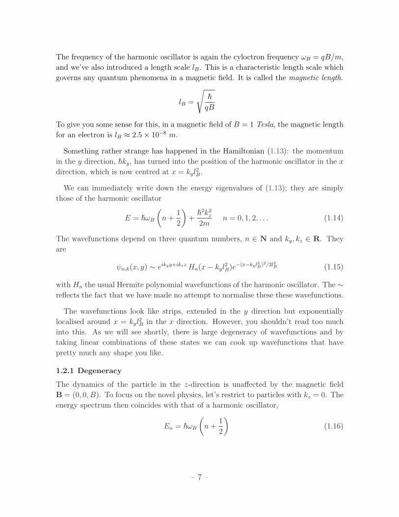
The frequency of the harmonic oscillator is again the cyloctron frequency ωB = qB/m,

and we’ve also introduced a length scale lB. This is a characteristic length scale which

governs any quantum phenomena in a magnetic field. It is called the magnetic length.

lB =

√~qB

To give you some sense for this, in a magnetic field of B = 1 Tesla, the magnetic length

for an electron is lB ≈ 2.5× 10−8 m.

Something rather strange has happened in the Hamiltonian (1.13): the momentum

in the y direction, ~ky, has turned into the position of the harmonic oscillator in the x

direction, which is now centred at x = kyl2B.

We can immediately write down the energy eigenvalues of (1.13); they are simply

those of the harmonic oscillator

E = ~ωB(n+

1

2

)+

~2k2z

2mn = 0, 1, 2, . . . (1.14)

The wavefunctions depend on three quantum numbers, n ∈ N and ky, kz ∈ R. They

are

ψn,k(x, y) ∼ eikyy+ikzzHn(x− kyl2B)e−(x−kyl2B)2/2l2B (1.15)

with Hn the usual Hermite polynomial wavefunctions of the harmonic oscillator. The ∼reflects the fact that we have made no attempt to normalise these these wavefunctions.

The wavefunctions look like strips, extended in the y direction but exponentially

localised around x = kyl2B in the x direction. However, you shouldn’t read too much

into this. As we will see shortly, there is large degeneracy of wavefunctions and by

taking linear combinations of these states we can cook up wavefunctions that have

pretty much any shape you like.

1.2.1 Degeneracy

The dynamics of the particle in the z-direction is unaffected by the magnetic field

B = (0, 0, B). To focus on the novel physics, let’s restrict to particles with kz = 0. The

energy spectrum then coincides with that of a harmonic oscillator,

En = ~ωB(n+

1

2

)(1.16)

– 7 –

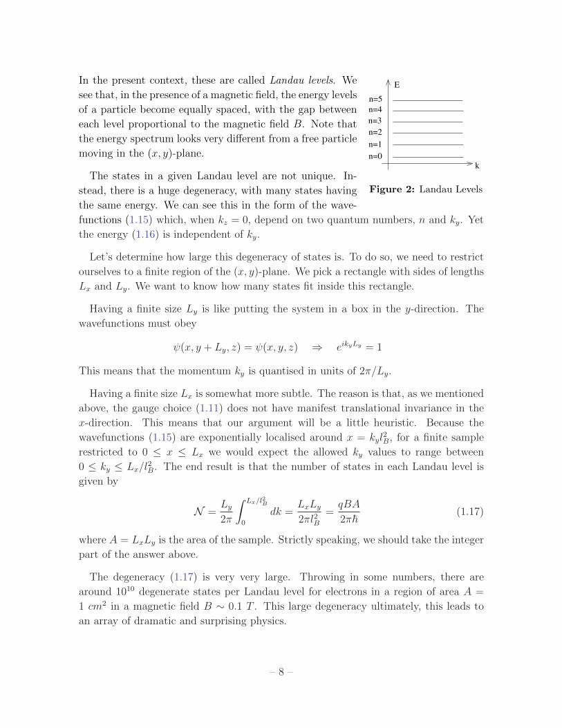
In the present context, these are called Landau levels. WeE

k

n=1

n=2

n=3

n=4

n=5

n=0

Figure 2: Landau Levels

see that, in the presence of a magnetic field, the energy levels

of a particle become equally spaced, with the gap between

each level proportional to the magnetic field B. Note that

the energy spectrum looks very different from a free particle

moving in the (x, y)-plane.

The states in a given Landau level are not unique. In-

stead, there is a huge degeneracy, with many states having

the same energy. We can see this in the form of the wave-

functions (1.15) which, when kz = 0, depend on two quantum numbers, n and ky. Yet

the energy (1.16) is independent of ky.

Let’s determine how large this degeneracy of states is. To do so, we need to restrict

ourselves to a finite region of the (x, y)-plane. We pick a rectangle with sides of lengths

Lx and Ly. We want to know how many states fit inside this rectangle.

Having a finite size Ly is like putting the system in a box in the y-direction. The

wavefunctions must obey

ψ(x, y + Ly, z) = ψ(x, y, z) ⇒ eikyLy = 1

This means that the momentum ky is quantised in units of 2π/Ly.

Having a finite size Lx is somewhat more subtle. The reason is that, as we mentioned

above, the gauge choice (1.11) does not have manifest translational invariance in the

x-direction. This means that our argument will be a little heuristic. Because the

wavefunctions (1.15) are exponentially localised around x = kyl2B, for a finite sample

restricted to 0 ≤ x ≤ Lx we would expect the allowed ky values to range between

0 ≤ ky ≤ Lx/l2B. The end result is that the number of states in each Landau level is

given by

N =Ly2π

∫ Lx/l2B

0

dk =LxLy2πl2B

=qBA

2π~(1.17)

where A = LxLy is the area of the sample. Strictly speaking, we should take the integer

part of the answer above.

The degeneracy (1.17) is very very large. Throwing in some numbers, there are

around 1010 degenerate states per Landau level for electrons in a region of area A =

1 cm2 in a magnetic field B ∼ 0.1 T . This large degeneracy ultimately, this leads to

an array of dramatic and surprising physics.

– 8 –

1.2.2 Symmetric Gauge

It is worthwhile to repeat the calculations above using a different gauge choice. This

will give us a slightly different perspective on the physics. A natural choice is symmetric

gauge

A = −1

2x×B =

B

2(−y, x, 0) (1.18)

This choice of gauge breaks translational symmetry in both the x and the y directions.

However, it does preserve rotational symmetry about the origin. This means that

angular momentum is now a good quantum number to label states.

In this gauge, the Hamiltonian is given by

H =1

2m

[(px +

qBy

2

)2

+

(py −

qBx

2

)2

+ p2z

]

= − ~2

2m∇2 +

qB

2mLz +

q2B2

8m(x2 + y2) (1.19)

where we’ve introduced the angular momentum operator

Lz = xpy − ypx

We’ll again restrict to motion in the (x, y)-plane, so we focus on states with kz = 0.

It turns out that complex variables are particularly well suited to describing states in

symmetric gauge, in particular in the lowest Landau level with n = 0. We define

w = x+ iy and w = x− iy

Correspondingly, the complex derivatives are

∂ =1

2

(∂

∂x− i ∂

∂y

)and ∂ =

1

2

(∂

∂x+ i

∂

∂y

)which obey ∂w = ∂w = 1 and ∂w = ∂w = 0. The Hamiltonian, restricted to states

with kz = 0, is then given by

H = −2~2

m∂∂ − ωB

2Lz +

mω2B

8ww

where now

Lz = ~(w∂ − w∂)

– 9 –

It is simple to check that the states in the lowest Landau level take the form

ψ0(w, w) = f(w)e−|w|2/4l2B

for any holomorphic function f(w). These all obey

Hψ0(w, w) =~ωB

2ψ0(w, w)

which is the statement that they lie in the lowest Landau level with n = 0. We can

further distinguish these states by requiring that they are also eigenvalues of Lz. These

are satisfied by the monomials,

ψ0 = wMe−|w|2/4l2B ⇒ Lzψ0 = ~Mψ0 (1.20)

for some positive integer M .

Degeneracy Revisited

In symmetric gauge, the profiles of the wavefunctions (1.20) form concentric rings

around the origin. The higher the angular momentum M , the further out the ring.

This, of course, is very different from the strip-like wavefunctions that we saw in Landau

gauge (1.15). You shouldn’t read too much into this other than the fact that the profile

of the wavefunctions is not telling us anything physical as it is not gauge invariant.

However, it’s worth revisiting the degeneracy of states in symmetric gauge. The

wavefunction with angular momentum M is peaked on a ring of radius r =√

2MlB.

This means that in a disc shaped region of area A = πR2, the number of states is

roughly (the integer part of)

N = R2/2l2B = A/2πl2B =qBA

2π~which agrees with our earlier result (1.17).

1.2.3 An Invitation to the Quantum Hall Effect

Take a system with some fixed number of electrons, which are restricted to move in

the (x, y)-plane. The charge of the electron is q = −e. In the presence of a magnetic

field, these will first fill up the N = eBA/2π~ states in the n = 0 lowest Landau level.

If any are left over they will then start to fill up the n = 1 Landau level, and so on.

Now suppose that we increase the magnetic field B. The number of states N housed

in each Landau level will increase, leading to a depletion of the higher Landau levels.

At certain, very special values of B, we will find some number of Landau levels that

are exactly filled. However, generically there will be a highest Landau level which is

only partially filled.

– 10 –

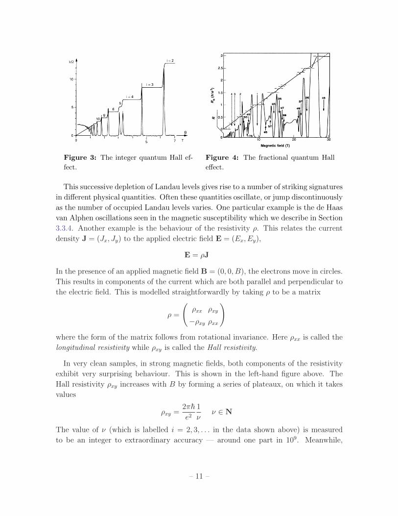
Figure 3: The integer quantum Hall ef-

fect.

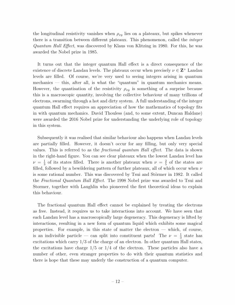
Figure 4: The fractional quantum Hall

effect.

This successive depletion of Landau levels gives rise to a number of striking signatures

in different physical quantities. Often these quantities oscillate, or jump discontinuously

as the number of occupied Landau levels varies. One particular example is the de Haas

van Alphen oscillations seen in the magnetic susceptibility which we describe in Section

3.3.4. Another example is the behaviour of the resistivity ρ. This relates the current

density J = (Jx, Jy) to the applied electric field E = (Ex, Ey),

E = ρJ

In the presence of an applied magnetic field B = (0, 0, B), the electrons move in circles.

This results in components of the current which are both parallel and perpendicular to

the electric field. This is modelled straightforwardly by taking ρ to be a matrix

ρ =

(ρxx ρxy

−ρxy ρxx

)where the form of the matrix follows from rotational invariance. Here ρxx is called the

longitudinal resistivity while ρxy is called the Hall resistivity.

In very clean samples, in strong magnetic fields, both components of the resistivity

exhibit very surprising behaviour. This is shown in the left-hand figure above. The

Hall resistivity ρxy increases with B by forming a series of plateaux, on which it takes

values

ρxy =2π~e2

1

νν ∈ N

The value of ν (which is labelled i = 2, 3, . . . in the data shown above) is measured

to be an integer to extraordinary accuracy — around one part in 109. Meanwhile,

– 11 –

the longitudinal resistivity vanishes when ρxy lies on a plateaux, but spikes whenever

there is a transition between different plateaux. This phenomenon, called the integer

Quantum Hall Effect, was discovered by Klaus von Klitzing in 1980. For this, he was

awarded the Nobel prize in 1985.

It turns out that the integer quantum Hall effect is a direct consequence of the

existence of discrete Landau levels. The plateaux occur when precisely ν ∈ Z+ Landau

levels are filled. Of course, we’re very used to seeing integers arising in quantum

mechanics — this, after all, is what the “quantum” in quantum mechanics means.

However, the quantisation of the resistivity ρxy is something of a surprise because

this is a macroscopic quantity, involving the collective behaviour of many trillions of

electrons, swarming through a hot and dirty system. A full understanding of the integer

quantum Hall effect requires an appreciation of how the mathematics of topology fits

in with quantum mechanics. David Thouless (and, to some extent, Duncan Haldane)

were awarded the 2016 Nobel prize for understanding the underlying role of topology

in this system.

Subsequently it was realised that similar behaviour also happens when Landau levels

are partially filled. However, it doesn’t occur for any filling, but only very special

values. This is referred to as the fractional quantum Hall effect. The data is shown

in the right-hand figure. You can see clear plateaux when the lowest Landau level has

ν = 13

of its states filled. There is another plateaux when ν = 25

of the states are

filled, followed by a bewildering pattern of further plateaux, all of which occur when ν

is some rational number. This was discovered by Tsui and Stormer in 1982. It called

the Fractional Quantum Hall Effect. The 1998 Nobel prize was awarded to Tsui and

Stormer, together with Laughlin who pioneered the first theoretical ideas to explain

this behaviour.

The fractional quantum Hall effect cannot be explained by treating the electrons

as free. Instead, it requires us to take interactions into account. We have seen that

each Landau level has a macroscopically large degeneracy. This degeneracy is lifted by

interactions, resulting in a new form of quantum liquid which exhibits some magical

properties. For example, in this state of matter the electron — which, of course,

is an indivisible particle — can split into constituent parts! The ν = 13

state has

excitations which carry 1/3 of the charge of an electron. In other quantum Hall states,

the excitations have charge 1/5 or 1/4 of the electron. These particles also have a

number of other, even stranger properties to do with their quantum statistics and

there is hope that these may underly the construction of a quantum computer.

– 12 –

We will not delve into any further details of the quantum Hall effect. Suffice to say

that it is one of the richest and most beautiful subjects in theoretical physics. You can

find a fuller exploration of these ideas in the lecture notes devoted to the Quantum

Hall Effect.

1.3 The Aharonov-Bohm Effect

In our course on Electromagnetism, we learned that the gauge potential Aµ is unphys-

ical: the physical quantities that affect the motion of a particle are the electric and

magnetic fields. Yet we’ve seen above that we cannot formulate quantum mechanics

without introducing the gauge fields A and φ. This might lead us to wonder whether

there is more to life than E and B alone. In this section we will see that things are,

indeed, somewhat more subtle.

1.3.1 Particles Moving around a Flux Tube

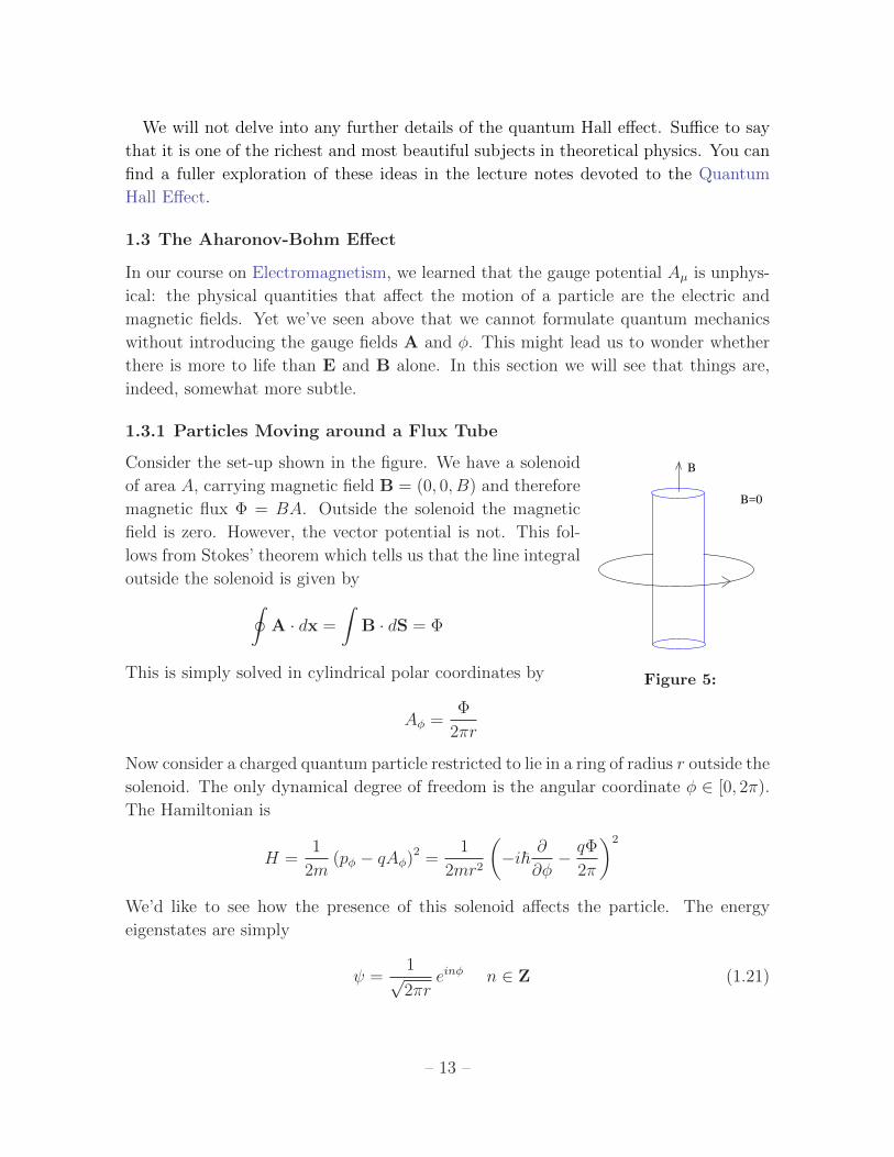
Consider the set-up shown in the figure. We have a solenoid

B=0

B

Figure 5:

of area A, carrying magnetic field B = (0, 0, B) and therefore

magnetic flux Φ = BA. Outside the solenoid the magnetic

field is zero. However, the vector potential is not. This fol-

lows from Stokes’ theorem which tells us that the line integral

outside the solenoid is given by∮A · dx =

∫B · dS = Φ

This is simply solved in cylindrical polar coordinates by

Aφ =Φ

2πr

Now consider a charged quantum particle restricted to lie in a ring of radius r outside the

solenoid. The only dynamical degree of freedom is the angular coordinate φ ∈ [0, 2π).

The Hamiltonian is

H =1

2m(pφ − qAφ)2 =

1

2mr2

(−i~ ∂

∂φ− qΦ

2π

)2

We’d like to see how the presence of this solenoid affects the particle. The energy

eigenstates are simply

ψ =1√2πr

einφ n ∈ Z (1.21)

– 13 –

Φ

E

n=1 n=2n=0

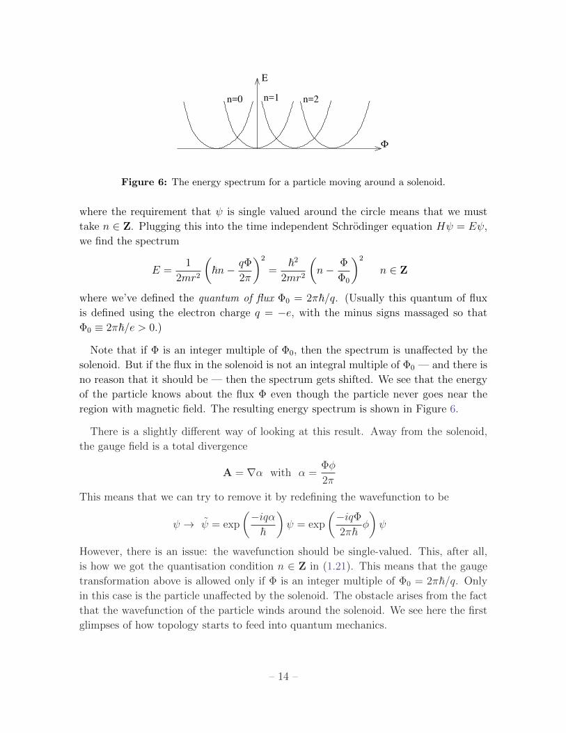
Figure 6: The energy spectrum for a particle moving around a solenoid.

where the requirement that ψ is single valued around the circle means that we must

take n ∈ Z. Plugging this into the time independent Schrodinger equation Hψ = Eψ,

we find the spectrum

E =1

2mr2

(~n− qΦ

2π

)2

=~2

2mr2

(n− Φ

Φ0

)2

n ∈ Z

where we’ve defined the quantum of flux Φ0 = 2π~/q. (Usually this quantum of flux

is defined using the electron charge q = −e, with the minus signs massaged so that

Φ0 ≡ 2π~/e > 0.)

Note that if Φ is an integer multiple of Φ0, then the spectrum is unaffected by the

solenoid. But if the flux in the solenoid is not an integral multiple of Φ0 — and there is

no reason that it should be — then the spectrum gets shifted. We see that the energy

of the particle knows about the flux Φ even though the particle never goes near the

region with magnetic field. The resulting energy spectrum is shown in Figure 6.

There is a slightly different way of looking at this result. Away from the solenoid,

the gauge field is a total divergence

A = ∇α with α =Φφ

2π

This means that we can try to remove it by redefining the wavefunction to be

ψ → ψ = exp

(−iqα~

)ψ = exp

(−iqΦ2π~

φ

)ψ

However, there is an issue: the wavefunction should be single-valued. This, after all,

is how we got the quantisation condition n ∈ Z in (1.21). This means that the gauge

transformation above is allowed only if Φ is an integer multiple of Φ0 = 2π~/q. Only

in this case is the particle unaffected by the solenoid. The obstacle arises from the fact

that the wavefunction of the particle winds around the solenoid. We see here the first

glimpses of how topology starts to feed into quantum mechanics.

– 14 –

There are a number of further lessons lurking in this simple quantum mechanical

set-up. You can read about them in the lectures on the Quantum Hall Effect (see

Section 1.5.3) and the lectures on Gauge Theory (see Section 3.6.1).

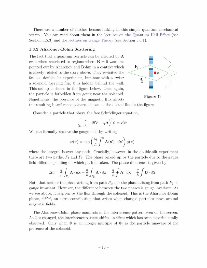
1.3.2 Aharonov-Bohm Scattering

The fact that a quantum particle can be affected by A

φ

P

1P

2

Figure 7:

even when restricted to regions where B = 0 was first

pointed out by Aharonov and Bohm in a context which

is closely related to the story above. They revisited the

famous double-slit experiment, but now with a twist:

a solenoid carrying flux Φ is hidden behind the wall.

This set-up is shown in the figure below. Once again,

the particle is forbidden from going near the solenoid.

Nonetheless, the presence of the magnetic flux affects

the resulting interference pattern, shown as the dotted line in the figure.

Consider a particle that obeys the free Schrodinger equation,

1

2m

(− i~∇− qA

)2

ψ = Eψ

We can formally remove the gauge field by writing

ψ(x) = exp

(iq

~

∫ x

A(x′) · dx′)φ(x)

where the integral is over any path. Crucially, however, in the double-slit experiment

there are two paths, P1 and P2. The phase picked up by the particle due to the gauge

field differs depending on which path is taken. The phase difference is given by

∆θ =q

~

∫P1

A · dx− q

~

∫P2

A · dx =q

~

∮A · dx =

q

~

∫B · dS

Note that neither the phase arising from path P1, nor the phase arising from path P2, is

gauge invariant. However, the difference between the two phases is gauge invariant. As

we see above, it is given by the flux through the solenoid. This is the Aharonov-Bohm

phase, eiqΦ/~, an extra contribution that arises when charged particles move around

magnetic fields.

The Aharonov-Bohm phase manifests in the interference pattern seen on the screen.

As Φ is changed, the interference pattern shifts, an effect which has been experimentally

observed. Only when Φ is an integer multiple of Φ0 is the particle unaware of the

presence of the solenoid.

– 15 –

1.4 Magnetic Monopoles

A magnetic monopole is a hypothetical object which emits a radial magnetic field of

the form

B =gr

4πr2⇒

∫dS ·B = g (1.22)

Here g is called the magnetic charge.

We learned in our first course on Electromagnetism that magnetic monopoles don’t

exist. First, and most importantly, they have never been observed. Second there’s a

law of physics which insists that they can’t exist. This is the Maxwell equation

∇ ·B = 0

Third, this particular Maxwell equation would appear to be non-negotiable. This is

because it follows from the definition of the magnetic field in terms of the gauge field

B = ∇×A ⇒ ∇ ·B = 0

Moreover, as we’ve seen above, the gauge field A is necessary to describe the quantum

physics of particles moving in magnetic fields. Indeed, the Aharonov-Bohm effect tells

us that there is non-local information stored in A that can only be detected by particles

undergoing closed loops. All of this points to the fact that we would be wasting our

time discussing magnetic monopoles any further.

Happily, there is a glorious loophole in all of these arguments, first discovered by

Dirac, and magnetic monopoles play a crucial role in our understanding of the more

subtle effects in gauge theories. The essence of this loophole is that there is an ambiguity

in how we define the gauge potentials. In this section, we will see how this arises.

1.4.1 Dirac Quantisation

It turns out that not any magnetic charge g is compatible with quantum mechanics.

Here we present several different arguments for the allowed values of g.

We start with the simplest and most physical of these arguments. Suppose that a

particle with charge q moves along some closed path C in the background of some gauge

potential A(x). Then, upon returning to its initial starting position, the wavefunction

of the particle picks up a phase

ψ → eiqα/~ψ with α =

∮C

A · dx (1.23)

This is the Aharonov-Bohm phase described above.

– 16 –

B

S

C

C

S’

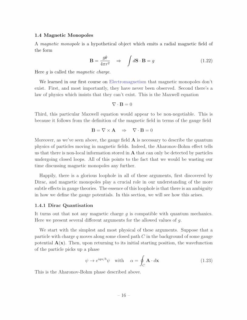
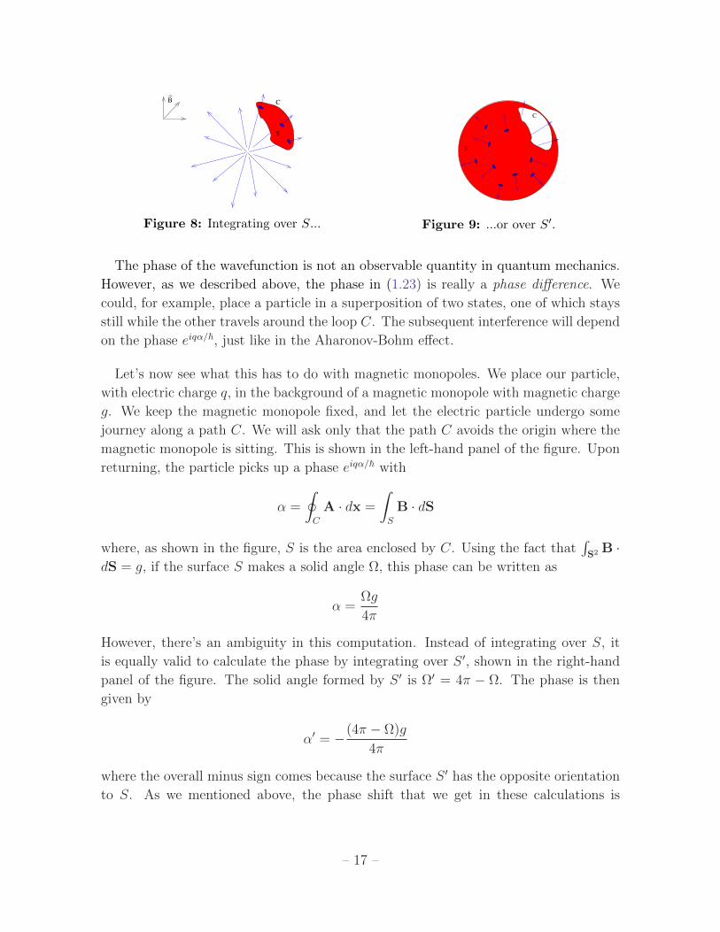
Figure 8: Integrating over S... Figure 9: ...or over S′.

The phase of the wavefunction is not an observable quantity in quantum mechanics.

However, as we described above, the phase in (1.23) is really a phase difference. We

could, for example, place a particle in a superposition of two states, one of which stays

still while the other travels around the loop C. The subsequent interference will depend

on the phase eiqα/~, just like in the Aharonov-Bohm effect.

Let’s now see what this has to do with magnetic monopoles. We place our particle,

with electric charge q, in the background of a magnetic monopole with magnetic charge

g. We keep the magnetic monopole fixed, and let the electric particle undergo some

journey along a path C. We will ask only that the path C avoids the origin where the

magnetic monopole is sitting. This is shown in the left-hand panel of the figure. Upon

returning, the particle picks up a phase eiqα/~ with

α =

∮C

A · dx =

∫S

B · dS

where, as shown in the figure, S is the area enclosed by C. Using the fact that∫

S2 B ·dS = g, if the surface S makes a solid angle Ω, this phase can be written as

α =Ωg

4π

However, there’s an ambiguity in this computation. Instead of integrating over S, it

is equally valid to calculate the phase by integrating over S ′, shown in the right-hand

panel of the figure. The solid angle formed by S ′ is Ω′ = 4π − Ω. The phase is then

given by

α′ = −(4π − Ω)g

4π

where the overall minus sign comes because the surface S ′ has the opposite orientation

to S. As we mentioned above, the phase shift that we get in these calculations is

– 17 –

observable: we can’t tolerate different answers from different calculations. This means

that we must have eiqα/~ = eiqα′/~. This gives the condition

qg = 2π~n with n ∈ Z (1.24)

This is the famous Dirac quantisation condition. The smallest such magnetic charge

has n = 1. It coincides with the quantum of flux, g = Φ0 = 2π~/q.

Above we worked with a single particle of charge q. Obviously, the same argument

must hold for any other particle of charge q′. There are two possibilities. The first is

that all particles carry charge that is an integer multiple of some smallest unit. In this

case, it’s sufficient to impose the Dirac quantisation condition (1.24) where q is the

smallest unit of charge. For example, in our world we should take q = ±e to be the

electron or proton charge (or, if we look more closely in the Standard Model, we might

choose to take q = −e/3, the charge of the down quark).

The second possibility is that the particles carry electric charges which are irrational

multiples of each other. For example, there may be a particle with charge q and another

particle with charge√

2q. In this case, no magnetic monopoles are allowed.

It’s sometimes said that the existence of a magnetic monopole would imply the

quantisation of electric charges. This, however, has it backwards. (It also misses the

point that we have a wonderful explanation of the quantisation of charges from the

story of anomaly cancellation in the Standard Model.) There are two possible groups

that could underly gauge transformations in electromagnetism. The first is U(1); this

has integer valued charges and admits magnetic monopoles. The second possibility is

R; this has irrational electric charges and forbids monopoles. All the evidence in our

world points to the fact that electromagnetism is governed by U(1) and that magnetic

monopoles should exist.

Above we looked at an electrically charged particle moving in the background of

a magnetically charged particle. It is simple to generalise the discussion to particles

that carry both electric and magnetic charges. These are called dyons. For two dyons,

with charges (q1, g1) and (q2, g2), the generalisation of the Dirac quantisation condition

requires

q1g2 − q2g1 ∈ 2π~Z

This is sometimes called the Dirac-Zwanziger condition.

– 18 –

1.4.2 A Patchwork of Gauge Fields

The discussion above shows how quantum mechanics constrains the allowed values of

magnetic charge. It did not, however, address the main obstacle to constructing a

magnetic monopole out of gauge fields A when the condition B = ∇×A would seem

to explicitly forbid such objects.

Let’s see how to do this. Our goal is to write down a configuration of gauge fields

which give rise to the magnetic field (1.22) of a monopole which we will place at the

origin. However, we will need to be careful about what we want such a gauge field to

look like.

The first point is that we won’t insist that the gauge field is well defined at the origin.

After all, the gauge fields arising from an electron are not well defined at the position of

an electron and it would be churlish to require more from a monopole. This fact gives

us our first bit of leeway, because now we need to write down gauge fields on R3/0,as opposed to R3 and the space with a point cut out enjoys some non-trivial topology

that we will make use of.

Consider the following gauge connection, written in spherical polar coordinates

ANφ =g

4πr

1− cos θ

sin θ(1.25)

The resulting magnetic field is

B = ∇×A =1

r sin θ

∂

∂θ(ANφ sin θ) r− 1

r

∂

∂r(rANφ )θ

Substituting in (1.25) gives

B =gr

4πr2(1.26)

In other words, this gauge field results in the magnetic monopole. But how is this

possible? Didn’t we learn in kindergarten that if we can write B = ∇ × A then∫dS ·B = 0? How does the gauge potential (1.25) manage to avoid this conclusion?

The answer is that AN in (1.25) is actually a singular gauge connection. It’s not just

singular at the origin, where we’ve agreed this is allowed, but it is singular along an

entire half-line that extends from the origin to infinity. This is due to the 1/ sin θ term

which diverges at θ = 0 and θ = π. However, the numerator 1− cos θ has a zero when

θ = 0 and the gauge connection is fine there. But the singularity along the half-line

θ = π remains. The upshot is that this gauge connection is not acceptable along the

line of the south pole, but is fine elsewhere. This is what the superscript N is there to

remind us: we can work with this gauge connection s long as we keep north.

– 19 –

Now consider a different gauge connection

ASφ = − g

4πr

1 + cos θ

sin θ(1.27)

This again gives rise to the magnetic field (1.26). This time it is well behaved at θ = π,

but singular at the north pole θ = 0. The superscript S is there to remind us that this

connection is fine as long as we keep south.

At this point, we make use of the ambiguity in the gauge connection. We are going

to take AN in the northern hemisphere and AS in the southern hemisphere. This is

allowed because the two gauge potentials are the same up to a gauge transformation,

A → A + ∇α. Recalling the expression for ∇α in spherical polars, we find that for

θ 6= 0, π, we can indeed relate ANφ and ASφ by a gauge transformation,

ANφ = ASφ +1

r sin θ∂φα where α =

gφ

2π(1.28)

However, there’s still a question remaining: is this gauge transformation allowed? The

problem is that the function α is not single valued: α(φ = 2π) = α(φ = 0) + g. And

this should concern us because, as we’ve seen in (1.8), the gauge transformation also

acts on the wavefunction of a quantum particle

ψ → eiqα/~ψ

There’s no reason that we should require the gauge transformation α to be single-

valued, but we do want the wavefunction ψ to be single-valued. This holds for the

gauge transformation (1.28) provided that we have

qg = 2π~n with n ∈ Z

This, of course, is the Dirac quantisation condition (1.24).

Mathematically, we have constructed of a topologically non-trivial U(1) bundle over

the S2 surrounding the origin. In this context, the integer n is called the first Chern

number.

1.4.3 Monopoles and Angular Momentum

Here we provide yet another derivation of the Dirac quantisation condition, this time

due to Saha. The key idea is that the quantisation of magnetic charge actually follows

from the more familiar quantisation of angular momentum. The twist is that, in the

presence of a magnetic monopole, angular momentum isn’t quite what you thought.

– 20 –

To set the scene, let’s go back to the Lorentz force law

dp

dt= q x×B

with p = mx. Recall from our discussion in Section 1.1.1 that p defined here is not

the canonical momentum, a fact which is hiding in the background in the following

derivation. Now let’s consider this equation in the presence of a magnetic monopole,

with

B =g

4π

r

r3

The monopole has rotational symmetry so we would expect that the angular momen-

tum, x× p, is conserved. Let’s check:

d(x× p)

dt= x× p + x× p = x× p = qx× (x×B)

=qg

4πr3x× (x× x) =

qg

4π

(x

r− rx

r2

)=

d

dt

( qg4π

r)

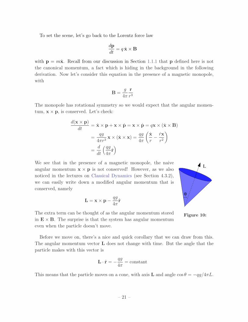
We see that in the presence of a magnetic monopole, the naiveL

θ

Figure 10:

angular momentum x × p is not conserved! However, as we also

noticed in the lectures on Classical Dynamics (see Section 4.3.2),

we can easily write down a modified angular momentum that is

conserved, namely

L = x× p− qg

4πr

The extra term can be thought of as the angular momentum stored

in E ×B. The surprise is that the system has angular momentum

even when the particle doesn’t move.

Before we move on, there’s a nice and quick corollary that we can draw from this.

The angular momentum vector L does not change with time. But the angle that the

particle makes with this vector is

L · r = − qg4π

= constant

This means that the particle moves on a cone, with axis L and angle cos θ = −qg/4πL.

– 21 –

So far, our discussion has been classical. Now we invoke some simple quantum

mechanics: the angular momentum should be quantised. In particular, the angular

momentum in the z-direction should be Lz ∈ 12~Z. Using the result above, we have

qg

4π=

1

2~n ⇒ qg = 2π~n with n ∈ Z

Once again, we find the Dirac quantisation condition.

1.5 Spin in a Magnetic Field

As we’ve seen in previous courses, particles often carry an intrinsic angular momentum

called spin S. This spin is quantised in half-integer units. For examples, electrons have

spin 12

and their spin operator is written in terms of the Pauli matrices σ,

S =~2σ

Importantly, the spin of any particle couples to a background magnetic field B. The

key idea here is that the intrinsic spin acts like a magnetic moment m which couples

to the magnetic field through the Hamiltonian

H = −m ·B

The question we would like to answer is: what magnetic moment m should we associate

with spin?

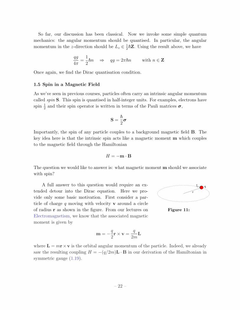
A full answer to this question would require an ex-

r

qv

Figure 11:

tended detour into the Dirac equation. Here we pro-

vide only some basic motivation. First consider a par-

ticle of charge q moving with velocity v around a circle

of radius r as shown in the figure. From our lectures on

Electromagnetism, we know that the associated magnetic

moment is given by

m = −q2r× v =

q

2mL

where L = mr×v is the orbital angular momentum of the particle. Indeed, we already

saw the resulting coupling H = −(q/2m)L ·B in our derivation of the Hamiltonian in

symmetric gauge (1.19).

– 22 –

Since the spin of a particle is another contribution to the angular momentum, we

might anticipate that the associated magnetic moment takes the form

m = gq

2mS

where g is some dimensionless number. (Note: g is unrelated to the magnetic charge

that we discussed in the previous section!) This, it turns out, is the right answer.

However, the value of g depends on the particle under consideration. The upshot is

that we should include a term in the Hamiltonian of the form

H = −g q

2mS ·B (1.29)

The g-factor

For fundamental particles with spin 12

— such as the electron — there is a long and

interesting history associated to determining the value of g. For the electron, this was

first measured experimentally to be

ge = 2

Soon afterwards, Dirac wrote down his famous relativistic equation for the electron.

One of its first successes was the theoretical prediction ge = 2 for any spin 12

particle.

This means, for example, that the neutrinos and quarks also have g = 2.

This, however, was not the end of the story. With the development of quantum field

theory, it was realised that there are corrections to the value ge = 2. These can be

calculated and take the form of a series expansion, starting with

ge = 2(

1 +α

2π+ . . .

)≈ 2.00232

where α = e2/4πε0~c ≈ 1/137 is the dimensionless fine structure constant which char-

acterises the strength of the Coulomb force. The most accurate experimental measure-

ment of the electron magnetic moment now yields the result

ge ≈ 2.00231930436182± 2.6× 10−13

Theoretical calculations agree to the first ten significant figures or so. This is the most

impressive agreement between theory and experiment in all of science! Beyond that,

the value of α is not known accurately enough to make a comparison. Indeed, now

the measurement of the electron magnetic moment is used to define the fine structure

constant α.

– 23 –

While all fundamental spin 12

particles have g ≈ 2, this does not hold for more

complicated objects. For example, the proton has

gp ≈ 5.588

while the neutron — which of course, is a neutral particle, but still carries a magnetic

moment — has

gn ≈ −3.823

where, because the neutron is neutral, the charge q = e is used in the formula (1.29).

These measurements were one of the early hints that the proton and neutron are com-

posite objects.

1.5.1 Spin Precession

Consider a constant magnetic field B = (0, 0, B). We would like to understand how

this affects the spin of an electron. We’ll take ge = 2. We write the electric charge of

the electron as q = −e so the Hamiltonian is

H =e~2m

σ ·B

The eigenstates are simply the spin-up |↑ 〉 and spin-down |↓ 〉 states in the z-direction.

They have energies

H|↑ 〉 =~ωB

2|↑ 〉 and H|↓ 〉 = −~ωB

2|↓ 〉

where ωB = eB/m is the cyclotron frequency which appears throughout this chapter.

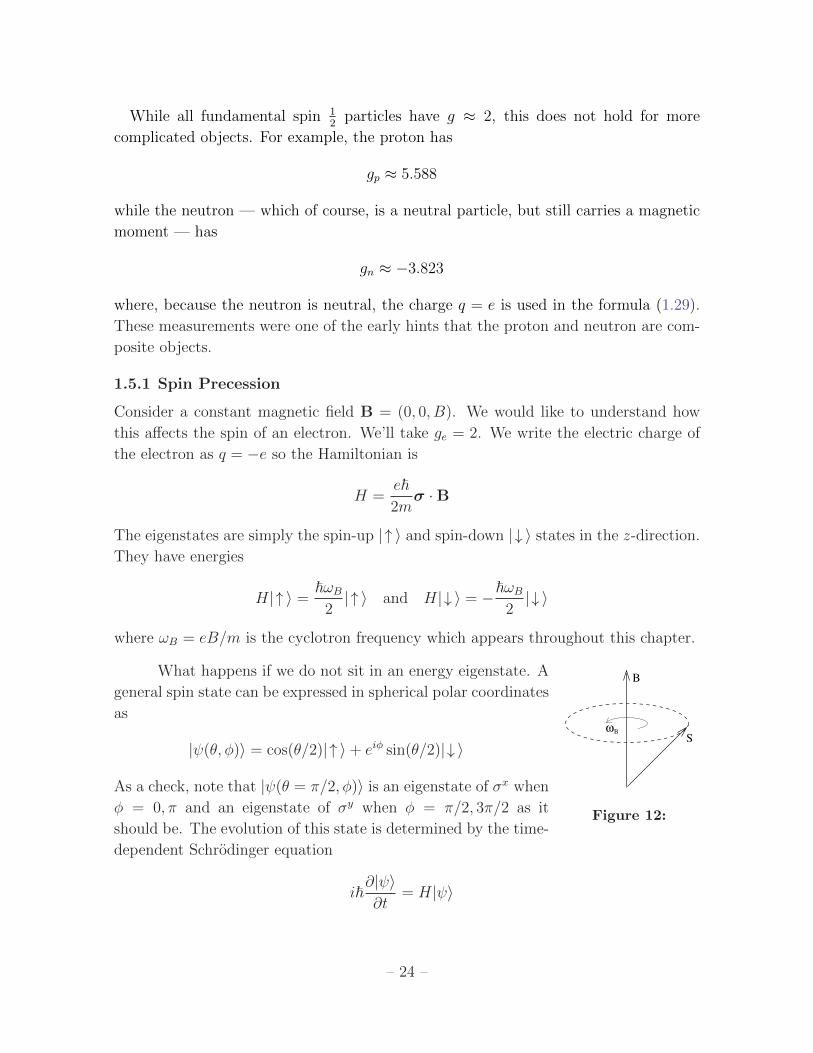
What happens if we do not sit in an energy eigenstate. A

ωB

B

S

Figure 12:

general spin state can be expressed in spherical polar coordinates

as

|ψ(θ, φ)〉 = cos(θ/2)|↑ 〉+ eiφ sin(θ/2)|↓ 〉

As a check, note that |ψ(θ = π/2, φ)〉 is an eigenstate of σx when

φ = 0, π and an eigenstate of σy when φ = π/2, 3π/2 as it

should be. The evolution of this state is determined by the time-

dependent Schrodinger equation

i~∂|ψ〉∂t

= H|ψ〉

– 24 –

which is easily solved to give

|ψ(θ, φ; t)〉 = eiωBt/2[

cos(θ/2)|↑ 〉+ ei(φ−ωBt) sin(θ/2)|↓ 〉]

We see that the effect of the magnetic field is to cause the spin to precess about the B

axis, as shown in the figure.

1.5.2 A First Look at the Zeeman Effect

The Zeeman effect describes the splitting of atomic energy levels in the presence of a

magnetic field. Consider, for example, the hydrogen atom with Hamiltonian

H = − ~2

2m∇2 − 1

4πε0

e2

r

The energy levels are given by

En = −α2mc2

2

1

n2n ∈ Z

where α is the fine structure constant. Each energy level has a degeneracy of states.

These are labelled by the angular momentum l = 0, 1, . . . , n− 1 and the z-component

of angular momentum ml = −l, . . . ,+l. Furthermore, each electron carries one of two

spin states labelled by ms = ±12. This results in a degeneracy given by

Degeneracy = 2n−1∑l=0

(2l + 1) = 2n2

Now we add a magnetic field B = (0, 0, B). As we have seen, this results in perturbation

to the Hamiltonian which, to leading order in B, is given by

∆H =e

2m(L + geS) ·B

In the presence of such a magnetic field, the degeneracy of the states is split. The

energy levels now depend on the quantum numbers n, ml and ms and are given by

En,m,s = En +e

2m(ml + 2ms)B

The Zeeman effect is developed further in the Lectures on Topics in Quantum Mechanics.

– 25 –

2. Band Structure

In this chapter, we start our journey into the world of condensed matter physics. This

is the study of the properties of “stuff”. Here, our interest lies in a particular and

familiar kind of stuff: solids.

Solids are collections of tightly bound atoms. For most solids, these atoms arrange

themselves in regular patterns on an underlying crystalline lattice. Some of the elec-

trons of the atom then disassociate themselves from their parent atom and wander

through the lattice environment. The properties of these electrons determine many of

the properties of the solid, not least its ability to conduct electricity.

One might imagine that the electrons in a solid move in a fairly random fashion, as

they bounce from one lattice site to another, like a ball in a pinball machine. However,

as we will see, this is not at all the case: the more fluid nature of quantum particles

allows them to glide through a regular lattice, almost unimpeded, with a distorted

energy spectrum the only memory of the underlying lattice.

In this chapter, we will focus on understanding how the energy of an electron depends

on its momentum when it moves in a lattice environment. The usual formula for kinetic

energy, E = 12mv2 = p2/2m, is one of the first things we learn in theoretical physics as

children. As we will see, a lattice changes this in interesting ways, the consequences of

which we will explore in chapter 3.

2.1 Electrons Moving in One Dimension

We begin with some particularly simple toy models which capture much of the relevant

physics. These toy models describe an electron moving in a one-dimensional lattice.

We’ll take what lessons we can from this before moving onto more realistic descriptions

of electrons moving in higher dimensions.

2.1.1 The Tight-Binding Model

The tight-binding model is a caricature of electron motion in solid in which space is

made discrete. The electron can sit only on the locations of atoms in the solid and has

some small probability to hop to a neighbouring site due to quantum tunnelling.

To start with our “solid” consists of a one-dimensional lattice of atoms. This is

described by N points arranged along a line, each separated by distance a.

– 26 –

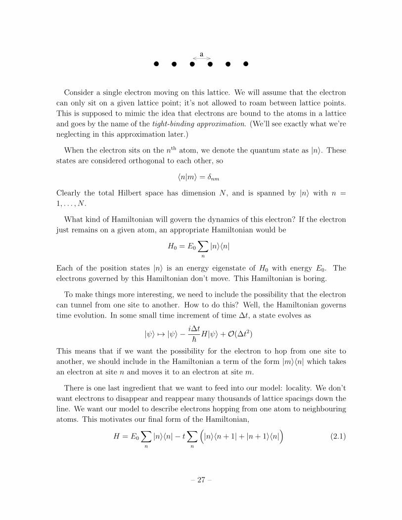
a

Consider a single electron moving on this lattice. We will assume that the electron

can only sit on a given lattice point; it’s not allowed to roam between lattice points.

This is supposed to mimic the idea that electrons are bound to the atoms in a lattice

and goes by the name of the tight-binding approximation. (We’ll see exactly what we’re

neglecting in this approximation later.)

When the electron sits on the nth atom, we denote the quantum state as |n〉. These

states are considered orthogonal to each other, so

〈n|m〉 = δnm

Clearly the total Hilbert space has dimension N , and is spanned by |n〉 with n =

1, . . . , N .

What kind of Hamiltonian will govern the dynamics of this electron? If the electron

just remains on a given atom, an appropriate Hamiltonian would be

H0 = E0

∑n

|n〉〈n|

Each of the position states |n〉 is an energy eigenstate of H0 with energy E0. The

electrons governed by this Hamiltonian don’t move. This Hamiltonian is boring.

To make things more interesting, we need to include the possibility that the electron

can tunnel from one site to another. How to do this? Well, the Hamiltonian governs

time evolution. In some small time increment of time ∆t, a state evolves as

|ψ〉 7→ |ψ〉 − i∆t

~H|ψ〉+O(∆t2)

This means that if we want the possibility for the electron to hop from one site to

another, we should include in the Hamiltonian a term of the form |m〉〈n| which takes

an electron at site n and moves it to an electron at site m.

There is one last ingredient that we want to feed into our model: locality. We don’t

want electrons to disappear and reappear many thousands of lattice spacings down the

line. We want our model to describe electrons hopping from one atom to neighbouring

atoms. This motivates our final form of the Hamiltonian,

H = E0

∑n

|n〉〈n| − t∑n

(|n〉〈n+ 1|+ |n+ 1〉〈n|

)(2.1)

– 27 –

First a comment on notation: the parameter t is called the hopping parameter. It is not

time; it is simply a number which determines the probability that a particle will hop

to a neighbouring site. (More precisely, the ratio t2/E20 will determine the probability.

of hopping.) It’s annoying notation, but unfortunately t is the canonical name for this

hopping parameter so it’s best we get used to it now.

Now back to the physics encoded in H. We’ve chosen a Hamiltonian that only

includes hopping terms between neighbouring sites. This is the simplest choice; we will

describe more general choices later. Moreover, the probability of hopping to the left is

the same as the probability of hopping to the right. This is required because H must

be a Hermitian operator.

There’s one final issue that we have to address before solving for the spectrum of H:

what happens at the edges? Again, there are a number of different possibilities but

none of the choices affect the physics that we’re interested in here. The simplest option

is simply to declare that the lattice is periodic. This is best achieved by introducing a

new state |N + 1〉, which sits to the right of |N〉, and is identified with |N + 1〉 ≡ |1〉.

Solving the Tight-Binding Model

Let’s now solve for the energy eigenstates of the Hamiltonian (2.1). A general state

can be expanded as

|ψ〉 =∑m

ψm|m〉

with ψn ∈ C. Substituting this into the Schrodinger equation gives

H|ψ〉 = E|ψ〉 ⇒ E0

∑m

ψm|m〉 − t(∑

m

ψm+1|m〉+ ψm|m+ 1〉)

= E∑n

ψm|m〉

If we now take the overlap with a given state 〈n|, we get the set of linear equations for

the coefficients ψn

〈n|H|ψ〉 = E〈n|ψ〉 ⇒ E0ψn − t(ψn+1 + ψn−1) = Eψn (2.2)

These kind of equations arise fairly often in physics. (Indeed, they will arise again in

Section 4 when we come to discuss the vibrations of a lattice.) They are solved by the

ansatz

ψn = eikna (2.3)

Or, if we want to ensure that the wavefunction is normalised, ψn = eikna/√N . The

exponent k is called the wavenumber. The quantity p = ~k plays a role similar to

momentum in our discrete model; we will discuss the ways in which it is like momentum

in Section 2.1.4. We’ll also often be lazy and refer to k as momentum.

– 28 –

The wavenumber has a number of properties. First, the set of solutions remain the

same if we shift k → k + 2π/a so the wavenumber takes values in

k ∈[−πa,+

π

a

)(2.4)

This range of k is given the fancy name Brillouin zone. We’ll see why this is a useful

concept that deserves its own name in Section 2.2.

There is also a condition on the allowed values of k coming from the requirement of

periodicity. We want ψN+1 = ψ1, which means that eikNa = 1. This requires that k

is quantised in units of 2π/aN . In other words, within the Brillouin zone (2.4) there

are exactly N quantum states of the form (2.3). But that’s what we expect as it’s the

dimension of our Hilbert space; the states (2.3) form a different basis.

States of the form (2.3) have the property that

-3 -2 -1 0 1 2 3

0

1

2

3

4

k

E(k)

Figure 13:

ψn±1 = e±ikaψn

This immediately ensures that equation (2.2) is

solved for any value of k, with the energy eigen-

value

E = E0 − 2t cos(ka) (2.5)

The spectrum is shown in the figure for t > 0.

(The plot was made with a = t = 1 and E0 = 2.) The states with k > 0 describe

electrons which move to the right; those with k < 0 describe electrons moving to the

left.

There is a wealth of physics hiding in this simple result, and much of the following

sections will be fleshing out these ideas. Here we highlight a few pertinent points

• The electrons do not like to sit still. The eigenstates |n〉 of the original Hamil-

tonian H0 were localised in space. One might naively think that adding a tiny

hopping parameter t would result in eigenstates that were spread over a few sites.

But this is wrong. Instead, all energy eigenstates are spread throughout the whole

lattice. Arbitrarily small local interactions result in completely delocalised energy

eigenstates.

• The energy eigenstates of H0 were completely degenerate. Adding the hopping

term lifts this degeneracy. Instead, the eigenstates are labelled by the wavevector

– 29 –

k and have energies (2.5) that lie in a range E(k) ∈ [E0 − 2t, E0 + 2t]. This

range of energies is referred to a band and the difference between the maximum

and minimum energy (which is 4t in this case) is called the band width. In our

simple model, we have just a single energy band. In subsequent models, we will

see multiple bands emerging.

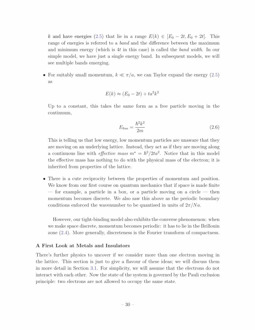
• For suitably small momentum, k π/a, we can Taylor expand the energy (2.5)

as

E(k) ≈ (E0 − 2t) + ta2k2

Up to a constant, this takes the same form as a free particle moving in the

continuum,

Efree =~2k2

2m(2.6)

This is telling us that low energy, low momentum particles are unaware that they

are moving on an underlying lattice. Instead, they act as if they are moving along

a continuous line with effective mass m? = ~2/2ta2. Notice that in this model

the effective mass has nothing to do with the physical mass of the electron; it is

inherited from properties of the lattice.

• There is a cute reciprocity between the properties of momentum and position.

We know from our first course on quantum mechanics that if space is made finite

— for example, a particle in a box, or a particle moving on a circle — then

momentum becomes discrete. We also saw this above as the periodic boundary

conditions enforced the wavenumber to be quantised in units of 2π/Na.

However, our tight-binding model also exhibits the converse phenomenon: when

we make space discrete, momentum becomes periodic: it has to lie in the Brillouin

zone (2.4). More generally, discreteness is the Fourier transform of compactness.

A First Look at Metals and Insulators

There’s further physics to uncover if we consider more than one electron moving in

the lattice. This section is just to give a flavour of these ideas; we will discuss them

in more detail in Section 3.1. For simplicity, we will assume that the electrons do not

interact with each other. Now the state of the system is governed by the Pauli exclusion

principle: two electrons are not allowed to occupy the same state.

– 30 –

As we have seen, our tight-binding model contains N states. However, each electron

has two internal states, spin |↑ 〉 and spin |↓ 〉. This means that, in total, each electron

can be in one of 2N different states. Invoking the Pauli exclusion principle, we see that

our tight-binding model makes sense as long as the number of electrons is less than or

equal to 2N .

The Pauli exclusion principle means that the ground state of a multi-electron system

has interesting properties. The first two electrons that we put in the system can both

sit in the lowest energy state with k = 0 as long as they have opposite spins. The next

electron that we put in finds these states occupied; it must sit in the next available

energy state which has k = ±2π/Na. And so this continues, with subsequent electrons

sitting in the lowest energy states which have not previously been occupied. The net

result is that the electrons fill all states up to some final kF which is known as the Fermi

momentum. The boundary between the occupied and unoccupied states in known as

the Fermi surface. Note that it is a surface in momentum space, rather than in real

space. We will describe this in more detail in Section 3.1. (See also the lectures on

Statistical Physics.)

How many electrons exist in a real material? Here something nice happens, because

the electrons which are hopping around the lattice come from the atoms themselves.

One sometimes talks about each atom “donating” an electron. Following our chemist

friends, these are called valence electrons. Given that our lattice contains N atoms,

it’s most natural to talk about the situation where the system contains ZN electrons,

with Z an integer. The atom is said to have valency Z.

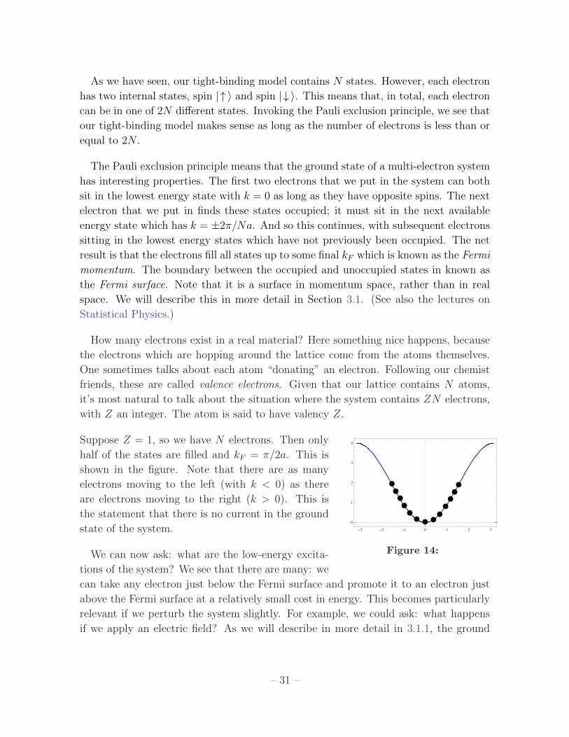
Suppose Z = 1, so we have N electrons. Then only

- - -

Figure 14:

half of the states are filled and kF = π/2a. This is

shown in the figure. Note that there are as many

electrons moving to the left (with k < 0) as there

are electrons moving to the right (k > 0). This is

the statement that there is no current in the ground

state of the system.

We can now ask: what are the low-energy excita-

tions of the system? We see that there are many: we

can take any electron just below the Fermi surface and promote it to an electron just

above the Fermi surface at a relatively small cost in energy. This becomes particularly

relevant if we perturb the system slightly. For example, we could ask: what happens

if we apply an electric field? As we will describe in more detail in 3.1.1, the ground

– 31 –

state of the system re-arranges itself at just a small cost of energy: some left-moving

states below the Fermi surface become unoccupied, while right-moving states above the

Fermi surface become occupied. Now, however, there are more electrons with k > 0

than with k < 0. This results in an electrical current. What we have just described is

a conductor.

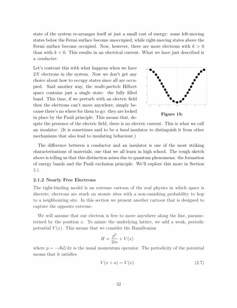
Let’s contrast this with what happens when we have

- - -

Figure 15:

2N electrons in the system. Now we don’t get any

choice about how to occupy states since all are occu-

pied. Said another way, the multi-particle Hilbert

space contains just a single state: the fully filled

band. This time, if we perturb with an electric field

then the electrons can’t move anywhere, simply be-

cause there’s no where for them to go: they are locked

in place by the Pauli principle. This means that, de-

spite the presence of the electric field, there is no electric current. This is what we call

an insulator. (It is sometimes said to be a band insulator to distinguish it from other

mechanisms that also lead to insulating behaviour.)

The difference between a conductor and an insulator is one of the most striking

characterisations of materials, one that we all learn in high school. The rough sketch

above is telling us that this distinction arises due to quantum phenomena: the formation

of energy bands and the Pauli exclusion principle. We’ll explore this more in Section

3.1.

2.1.2 Nearly Free Electrons

The tight-binding model is an extreme cartoon of the real physics in which space is

discrete; electrons are stuck on atomic sites with a non-vanishing probability to hop

to a neighbouring site. In this section we present another cartoon that is designed to

capture the opposite extreme.

We will assume that our electron is free to move anywhere along the line, parame-

terised by the position x. To mimic the underlying lattice, we add a weak, periodic

potential V (x). This means that we consider the Hamiltonian

H =p2

2m+ V (x)

where p = −i~d/dx is the usual momentum operator. The periodicity of the potential

means that it satisfies

V (x+ a) = V (x) (2.7)

– 32 –

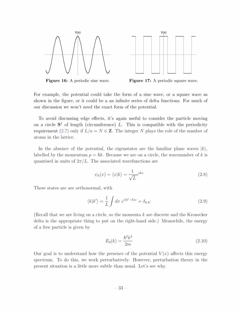
V(x) V(x)

Figure 16: A periodic sine wave. Figure 17: A periodic square wave.

For example, the potential could take the form of a sine wave, or a square wave as

shown in the figure, or it could be a an infinite series of delta functions. For much of

our discussion we won’t need the exact form of the potential.

To avoid discussing edge effects, it’s again useful to consider the particle moving

on a circle S1 of length (circumference) L. This is compatible with the periodicity

requirement (2.7) only if L/a = N ∈ Z. The integer N plays the role of the number of

atoms in the lattice.

In the absence of the potential, the eigenstates are the familiar plane waves |k〉,labelled by the momentum p = ~k. Because we are on a circle, the wavenumber of k is

quantised in units of 2π/L. The associated wavefunctions are

ψk(x) = 〈x|k〉 =1√Leikx (2.8)

These states are are orthonormal, with

〈k|k′〉 =1

L

∫dx ei(k

′−k)x = δk,k′ (2.9)

(Recall that we are living on a circle, so the momenta k are discrete and the Kronecker

delta is the appropriate thing to put on the right-hand side.) Meanwhile, the energy

of a free particle is given by

E0(k) =~2k2

2m(2.10)

Our goal is to understand how the presence of the potential V (x) affects this energy

spectrum. To do this, we work perturbatively. However, perturbation theory in the

present situation is a little more subtle than usual. Let’s see why.

– 33 –

Perturbation Theory

Recall that the first thing we usually do in perturbation theory is decide whether

we have non-degenerate or degenerate energy eigenstates. Which do we have in the

present case? Well, all states are trivially degenerate because the energy of a free

particle moving to the right is the same as the energy of a free particle moving to the

left: E0(k) = E0(−k). But the fact that the two states |k〉 and |−k〉 have the same

energy does not necessarily mean that we have to use degenerate perturbation theory.

This is only true if the perturbation causes the two states to mix.

To see what happens we will need to compute matrix elements 〈k|V |k′〉. The key bit

of physics is the statement that the potential is periodic (2.7). This ensures that it can

be Fourier expanded

V (x) =∑n∈Z

Vn e2πinx/a with Vn = V ?

−n

where the Fourier coefficients follow from the inverse transformation

Vn =1

a

∫ a

0

dx V (x) e−2πinx/a

The matrix elements are then given by

〈k|V |k′〉 =1

L

∫dx∑n∈Z

Vn ei(k′−k+2πn/a)x =

∑n∈Z

Vn δk−k′,2πn/a (2.11)

We see that we get mixing only when

k = k′ +2πn

a

for some integer n. In particular, we get mixing between degenerate states |k〉 and |−k〉only when

k =πn

a

for some n. The first time that this happens is when k = π/a. But we’ve seen this

value of momentum before: it is the edge of the Brillouin zone (2.4). This is the first

hint that the tight-binding model and nearly free electron model share some common

features.

With this background, let’s now try to sketch the basic features of the energy spec-

trum as a function of k.

– 34 –

Low Momentum: With low momentum |k| π/a, there is no mixing between states

at leading order in perturbation theory (and very little mixing at higher order). In

this regime we can use our standard results from non-degenerate perturbation theory.

Expanding the energy to second order, we have

E(k) =~2k2

2m+ 〈k|V |k〉+

∑k′ 6=k

|〈k|V |k′〉|2

E0(k)− E0(k′)+ . . . (2.12)

From (2.11), we know that the first order correction is 〈k|V |k〉 = V0, and so just

gives a constant shift to the energy, independent of k. Meanwhile, the second order

term only gets contributions from |k′〉 = |k + 2πn/a〉 for some n. When |k| π/a,

these corrections are small. We learn that, for small momenta, the particle moves as if

unaffected by the potential. Intuitively, the de Broglie wavelength 2π/k of the particle

much greater than the wavelength a of the potential, and the particle just glides over

it unimpeded.

The formula (2.12) holds for low momenta. It also holds for momenta πn/a k π(n + 1)/a which are far from the special points where mixing occurs. However,

the formula knows about its own failings because if we attempt to use it when k =

nπ/a for some n, the the numerator 〈k|V |−k〉 is finite while the denominator becomes

zero. Whenever perturbation theory diverges in this manner it’s because we’re doing

something wrong. In this case it’s because we should be working with degenerate

perturbation theory.

At the Edge of the Brillouin Zone: Let’s consider the momentum eigenstates which

sit right at the edge of the Brillouin zone, k = π/a, or at integer multiples

k =nπ

a

As we’ve seen, these are the values which mix due to the potential perturbation and

we must work with degenerate perturbation theory.

Let’s recall the basics of degenerate perturbation theory. We focus on the subsector of

the Hilbert space formed by the two degenerate states, in our case |k〉 and |k′〉 = |−k〉.To leading order in perturbation theory, the new energy eigenstates will be some linear

combination of these original states α|k〉 + β|k′〉. We would like to figure out what

choice of α and β will diagonalise the new Hamiltonian. There will be two such choices

since there must, at the end of the day, remain two energy eigenstates. To determine

the correct choice of these coefficients, we write the Schrodinger equation, restricted to

– 35 –

this subsector, in matrix form(〈k|H|k〉 〈k|H|k′〉〈k′|H|k〉 〈k′|H|k′〉

)(α

β

)= E

(α

β

)(2.13)

We’ve computed the individual matrix elements above: using the fact that the states

|k〉 are orthonormal (2.9), the unperturbed energy (2.10) and the potential matrix

elements (2.11), our eigenvalue equation becomes(E0(k) + V0 Vn

V ?n E0(k′) + V0

)(α

β

)= E

(α

β

)(2.14)

where, for the value k = −k′ = nπ/a of interest, E0(k) = E0(k′) = n2~2π2/2ma2. It’s

simple to determine the eigenvalues E of this matrix: they are given by the roots of

the quadratic equation

(E0(k) + V0 − E)2 − |Vn|2 = 0 ⇒ E =~2

2m

n2π2

a2+ V0 ± |Vn| (2.15)

This is important. We see that a gap opens up in the spectrum at the values k = ±nπ/a.

The size of the gap is proportional to 2|Vn|.

It’s simple to understand what’s going on here. Consider the simple potential

V = 2V1 cos

(2πx

a

)which gives rise to a gap only at k = ±π/a. The eigenvectors of the matrix are

(α, β) = (1,−1) and (α, β) = (1, 1), corresponding to the wavefunctions

ψ+(x) = 〈x|(|k〉+ |−k〉

)∼ cos

(πxa

)ψ−(x) = 〈x|

(|k〉 − |−k〉

)∼ sin

(πxa

)The density of electrons is proportional to |ψ±|2. Plotting these densities on top of the

potential, we see that ψ+ describes electrons that are gathered around the peaks of the

potential, while ψ− describes electrons gathered around the minima. It is no surprise

that the energy of ψ+ is higher than that of ψ−.

– 36 –

Close to the Edge of the Brillouin Zone: Now consider an electron with

k =nπ

a+ δ

for some small δ. As we’ve seen, the potential causes plane wave states to mix only if

their wavenumbers differ by some multiple of 2π/a. This means that |k〉 = |nπ/a+ δ〉will mix with |k′〉 = |−nπ/a+ δ〉. These states don’t quite have the same kinetic

energy, but they have very nearly the same kinetic energy. And, as we will see, the

perturbation due to the potential V will mean that these states still mix strongly.

To see this mixing, we need once again to solve the eigenvalue equation (2.13) or,

equivalently, (2.14). The eigenvalues are given by solutions to the quadratic equation(E0(k) + V0 − E

)(E0(k′) + V0 − E

)− |Vn|2 = 0 (2.16)

The only difference from our previous discussion is that E(k) and E(k′) are now given

by

E(k) =~2

2m

(nπa

+ δ)2

and E(k′) =~2

2m

(nπa− δ)2

and the quadratic equation (2.16) becomes(~2

2m

(n2π2

a2+ δ2

)+ V0 − E

)2

−(

~2

2m

2nπδ

a

)2

− |Vn|2 = 0

This equation has two solutions, E = E±, given by

E± =~2

2m

(n2π2

a2+ δ2

)+ V0 ±

√|Vn|2 +

(~2

2m

2nπδ

a

)2

We’re ultimately interested in this expression when δ is small, where we anticipate that

the effect of mixing will be important. But, as a sanity check, let’s first expand it in

the opposite regime, when we’re far from the edge of the Brillouin zone and δ is large

compared to the gap Vn. In this case, a little bit of algebra shows that the eigenvalues

can be written as

E± = E0(nπ/a± δ) + V0 ±|Vn|2

E0(nπ/a+ δ)− E0(nπ/a− δ)

But this coincides with the the expression that we got from second-order, non-degenerate

perturbation theory (2.12). (Or, more precisely, because we have kept just a single mix-

ing term in our discussion above we get just a single term in the sum in (2.12); for some

choice of potentials, keeping further terms may be important.)

– 37 –

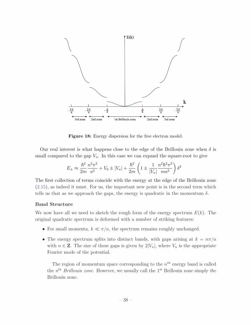
Figure 18: Energy dispersion for the free electron model.

Our real interest is what happens close to the edge of the Brillouin zone when δ is

small compared to the gap Vn. In this case we can expand the square-root to give

E± ≈~2

2m

n2π2

a2+ V0 ± |Vn|+

~2

2m

(1± 1

|Vn|n2~2π2

ma2

)δ2

The first collection of terms coincide with the energy at the edge of the Brillouin zone

(2.15), as indeed it must. For us, the important new point is in the second term which

tells us that as we approach the gaps, the energy is quadratic in the momentum δ.

Band Structure

We now have all we need to sketch the rough form of the energy spectrum E(k). The

original quadratic spectrum is deformed with a number of striking features:

• For small momenta, k π/a, the spectrum remains roughly unchanged.

• The energy spectrum splits into distinct bands, with gaps arising at k = nπ/a

with n ∈ Z. The size of these gaps is given by 2|Vn|, where Vn is the appropriate

Fourier mode of the potential.

The region of momentum space corresponding to the nth energy band is called

the nth Brillouin zone. However, we usually call the 1st Brillouin zone simply the

Brillouin zone.

– 38 –

• As we approach the edge of a band, the spectrum is quadratic. In particular,

dE/dk → 0 at the end of a band.

The relationship E(k) between energy and momentum is usually called the dispersion

relation. In the present case, it is best summarised in a figure.

Note that the spectrum within the first Brillouin zone |k| ≤ π/a, looks very similar to

what we saw in the tight-binding model . The qualitative differences in the two models

arise because the tight-binding model has a finite number of states, all contained in

the first Brillouin zone, while the nearly-free electron model has an infinite number of

states which continue for |k| > π/a.

2.1.3 The Floquet Matrix

One of the main lessons that we learned above is that there are gaps in the energy

spectrum. It’s hard to overstate the importance of these gaps. Indeed, as we saw

briefly above, and will describe in more detail in 3.1.1, the gaps are responsible for

some of the most prominent properties of materials, such as the distinction between

conductors and insulators.

Because of the important role they play, we will here describe another way to see the

emergence of gaps in the spectrum that does not rely on perturbation theory. Consider

a general, periodic potential V (x) = V (x + a). We are interested in solutions to the

Schrodinger equation

− ~2

2m

d2ψ

dx2+ V (x)ψ(x) = Eψ(x) (2.17)

Since this is a second order differential equation, we know that there must be two

solutions ψ1(x) and ψ2(x). However, because the potential is periodic, it must be the

case that ψ1(x + a) and ψ2(x + a) are also solutions. These two sets of solutions are

therefore related by some linear transformation(ψ1(x+ a)

ψ2(x+ a)

)= F (E)

(ψ1(x)

ψ2(x)

)(2.18)

where F (E) is a 2×2 matrix which, as the notation suggests, depends on the energy of

the solution E. It is known as the Floquet matrix and has a number of nice properties.

– 39 –

Claim: det(F ) = 1.

Proof: First some gymnastics. We differentiate (2.18) to get(ψ′1(x+ a)

ψ′2(x+ a)

)= F (E)

(ψ′1(x)

ψ′2(x)

)

We can combine this with our previous equation by introducing the 2× 2 matrix

W (x) =

(ψ1(x) ψ′1(x)

ψ2(x) ψ′2(x)

)

which obeys the matrix equation

W (x+ a) = F (E)W (x) (2.19)

Consider detW = ψ1ψ′2 − ψ′1ψ2. You might recognise this from the earlier course on

Differential Equations as the Wronskian. It’s simple to show, using the Schrodinger

equation (2.17), that (detW )′ = 0. This means that detW is independent of x so, in

particular, detW (x + a) = detW (x). Taking the determinant of (2.19) then tells us

that det F = 1 as claimed.

Claim: TrF is real.

Proof: We always have the choice pick the original wavefunctions ψ1(x) and ψ2(x)

to be entirely real for all x. (If they’re not, simply take the real part and this is also

a solution to the Schrodinger equation). With this choice, the Floquet matrix itself

has real elements, and so its trace is obviously real. But the trace is independent of

our choice of basis of wavefunctions. Any other choice is related by a transformation

F → AFA−1, for some invertible matrix A and this leaves the trace invariant. Hence,

even if the components of F (E) are complex, its trace remains real.

To understand the structure of solutions to (2.18), we look at the eigenvalues, λ+ and

λ− of F (E). Of course, these too depend on the energy E of the solutions. Because

detF = 1, they obey λ+λ− = 1. They obey the characteristic equation

λ2 − (TrF (E))λ+ 1 = 0

The kind of solution that we get depends on whether (TrF (E))2 < 4 or (TrF (E))2 > 4.

– 40 –

(TrF (E))2 < 4: In this case, the roots are complex and of equal magnitude. We can

write

λ+ = eika and λ− = e−ika

for some k which, assuming that the roots are distinct, lies in the range |k| < π/a.

To see what this means for solutions to (2.18), we introduce the left-eigenvector of

(α±, β±)F = λ±(α±, β±). Then the linear combinations ψ± = α±ψ1 + β±ψ2 obey

ψ±(x+ a) = e±ikaψ±(x)

These are extended states, spread (on average) equally throughout the lattice. They

corresponds to the bands in the spectrum.

(TrF (E))2 > 4: Now the eigenvalues take the form

λ1 = eµa and λ2 = e−µa

for some µ. The corresponding eigenstates now obey

ψ±(x+ a) = e±µaψ±(x)

States of this form are not allowed: they are unbounded either as x → +∞ or as

x→ −∞. These values of energy E are where the gaps occur in the spectrum.

We have to work a little harder when F (E) = 4 and the two eigenvalues are de-

generate, either both +1 or both −1. This situations corresponds to the edge of the

band. Consider the case when both eigenvalues are +1. Recall from your first course

on Vectors and Matrices that attempting to diagonalise such a 2× 2 matrix can result

in two different canonical forms

PF (E)P−1 =

(1 0

0 1

)or PF (E)P−1 =

(1 0

1 1

)

In the former case, there are two allowed solutions. In the latter case, you can check

that one solution is allowed, while the other grows linearly in x.

2.1.4 Bloch’s Theorem in One Dimension

In both models described above, we ended up labelling states by momentum ~k. It’s

worth pausing to ask: why did we do this? And how should we think of k?

– 41 –

Before we get to this, let’s back up and ask an even more basic question: why do

we label the states of a free particle by momentum? Here, the answer is because

momentum is conserved. In the quantum theory, this means that the momentum

operator commutes with the Hamiltonian: [p,H] = 0, so that we can simultaneously

label states by both energy and momentum. Ultimately, Noether’s theorem tells us

that this conservation law arises because of translational invariance of the system.

Now let’s look at our system with a lattice. We no longer have translational invari-

ance. Correspondingly, in the nearly-free electron model, [p,H] 6= 0. Hopefully this

now makes our original question sharper: why do we get to label states by k?!

While we don’t have full, continuous translational invariance, both the models that

we discussed do have a discrete version of translational invariance

x→ x+ a

As we now show, this is sufficient to ensure that we can label states by something very

similar to “momentum”. However, the values of this momentum are restricted. This

result is known as Bloch’s Theorem. Here we prove the theorem for our one-dimensional

system; we will revisit it in Section 2.3.1 in higher dimensions.

The Translation Operator

For concreteness, let’s work with continuous space where states are described by a

wavefunction ψ(x). (There is a simple generalisation to discrete situations such as the

tight-binding model that we describe below.) We introduce the translation operator Tlas

Tl ψ(x) = ψ(x+ l)

First note that Tl is a unitary operator. To see this, we just need to look at the overlap

〈φ|Tl|ψ〉 =

∫dx φ(x)? Tlψ(x) =

∫dx φ(x)?ψ(x+ l)

=

∫dx φ(x− l)?ψ(x) =

∫dx [T−l φ(x)]?ψ(x)

where, in the step to the second line, we’ve simply shifted the origin. This tells us that

T †l = T−l. But clearly T−1l = T−l as well, so T †l = T−1

l and the translation operator is

unitary as claimed.

– 42 –

Next note that the set of translation operators form an Abelian group,

Tl1Tl2 = Tl1+l2 (2.20)

with [Tl1 , Tl2 ] = 0.

The translation operator is a close cousin of the familiar momentum operator

p = −i~ ddx

The relationship between the two is as follows: the unitary translation operator is the

exponentiation of the Hermitian momentum operator

Tl = eilp/~

To see this, we expand the exponent and observe that Tlψ(x) = ψ(x + l) is just a

compact way of expressing the Taylor expansion of a function

Tlψ(x) =

(1 +

ilp

~+

1

2

(ilp

~

)2

+ . . .

)ψ(x)

=

(1 + l

d

dx+l2

2

d2

dx2+ . . .

)ψ(x) = ψ(x+ l)

We say that the momentum operator is the “generator” of infinitesimal translations.

A quantum system is said to be invariant under translations by l if

[H,Tl] = 0 (2.21)

Phrased in this way, we can describe both continuous translational symmetry and dis-

crete translational symmetry. A system has continuous translational invariance if (2.21)

holds for all l. In this case, we may equivalently say that [p,H] = 0. Alternatively,

a system may have discrete translational invariance if (2.21) holds only when l is an

integer multiple of the lattice spacing a. Now p does not commute with H.

Let’s look at the case of discrete symmetry. Now we can’t simultaneously diagonalise

p and H, but we can simultaneously diagonalise Ta and H. In other words, energy

eigenstates can be labelled by the eigenvalues of Ta. But Ta is a unitary operator and

its eigenvalues are simply a phase, eiθ for some θ. Moreover, we want the eigenvalues

to respect the group structure (2.20). This is achieved if we write the eigenvalue of Tl

– 43 –

as eiθ = eikl for some k, so that the eigenvalue of Tna coincides with the eigenvalue of

T na . The upshot is that eigenstates are labelled by some k, such that

Taψk(x) = ψk(x+ a) = eikaψk(x)

Now comes the rub. Because the eigenvalue is a phase, there is an arbitrariness in this

labelling: states labelled by k have the same eigenvalue under Ta as states labelled by

k + 2π/a. To remedy this, we will simply require that k lies in the range

k ∈[−πa,π

a

)(2.22)

We recognise this as the first Brillouin zone.

This, then, is the essence of physics on a lattice. We can still label states by k, but

it now lies in a finite range. Note that we can approximate a system with continuous

translational symmetry by taking a arbitrarily small; in this limit we get the usual

result k ∈ R.

This discussion leads us directly to:

Bloch’s Theorem in One Dimension: In a periodic potential, V (x) = V (x+ a),

there exists a basis of energy eigenstates that can be written as

ψk(x) = eikxuk(x)

where uk(x) = uk(x+ a) is a periodic function and k lies in the Brillouin zone (2.22).

Proof: We take ψk to be an eigenstate of the translation operator Ta, so that

ψk(x+ a) = eikaψk(x). Then uk(x+ a) = e−ik(x+a)ψk(x+ a) = e−ikxψk(x) = uk(x).

Bloch’s theorem is rather surprising. One might think that the presence of a periodic

potential would dramatically alter the energy eigenstates, perhaps localising them in

some region of space. Bloch’s theorem is telling us that this doesn’t happen: instead

the plane wave states eikx are altered only by a periodic function u(x), sometimes

referred to as a Bloch function, and the fact that the wavenumber is restricted to the

first Brillouin zone.

Finally, note that we’ve couched the above discussion in terms of wavefunctions ψ(x),

but everything works equally well for the tight-binding model with the translation

operator defined by Ta|n〉 = |n+ 1〉.

– 44 –

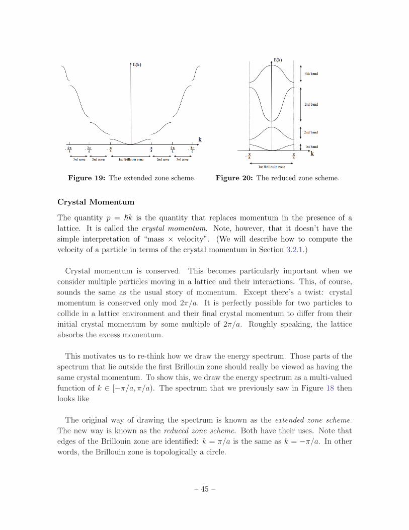
Figure 19: The extended zone scheme. Figure 20: The reduced zone scheme.

Crystal Momentum

The quantity p = ~k is the quantity that replaces momentum in the presence of a

lattice. It is called the crystal momentum. Note, however, that it doesn’t have the

simple interpretation of “mass × velocity”. (We will describe how to compute the

velocity of a particle in terms of the crystal momentum in Section 3.2.1.)

Crystal momentum is conserved. This becomes particularly important when we

consider multiple particles moving in a lattice and their interactions. This, of course,

sounds the same as the usual story of momentum. Except there’s a twist: crystal

momentum is conserved only mod 2π/a. It is perfectly possible for two particles to

collide in a lattice environment and their final crystal momentum to differ from their

initial crystal momentum by some multiple of 2π/a. Roughly speaking, the lattice

absorbs the excess momentum.

This motivates us to re-think how we draw the energy spectrum. Those parts of the

spectrum that lie outside the first Brillouin zone should really be viewed as having the

same crystal momentum. To show this, we draw the energy spectrum as a multi-valued

function of k ∈ [−π/a, π/a). The spectrum that we previously saw in Figure 18 then

looks like

The original way of drawing the spectrum is known as the extended zone scheme.

The new way is known as the reduced zone scheme. Both have their uses. Note that

edges of the Brillouin zone are identified: k = π/a is the same as k = −π/a. In other

words, the Brillouin zone is topologically a circle.

– 45 –

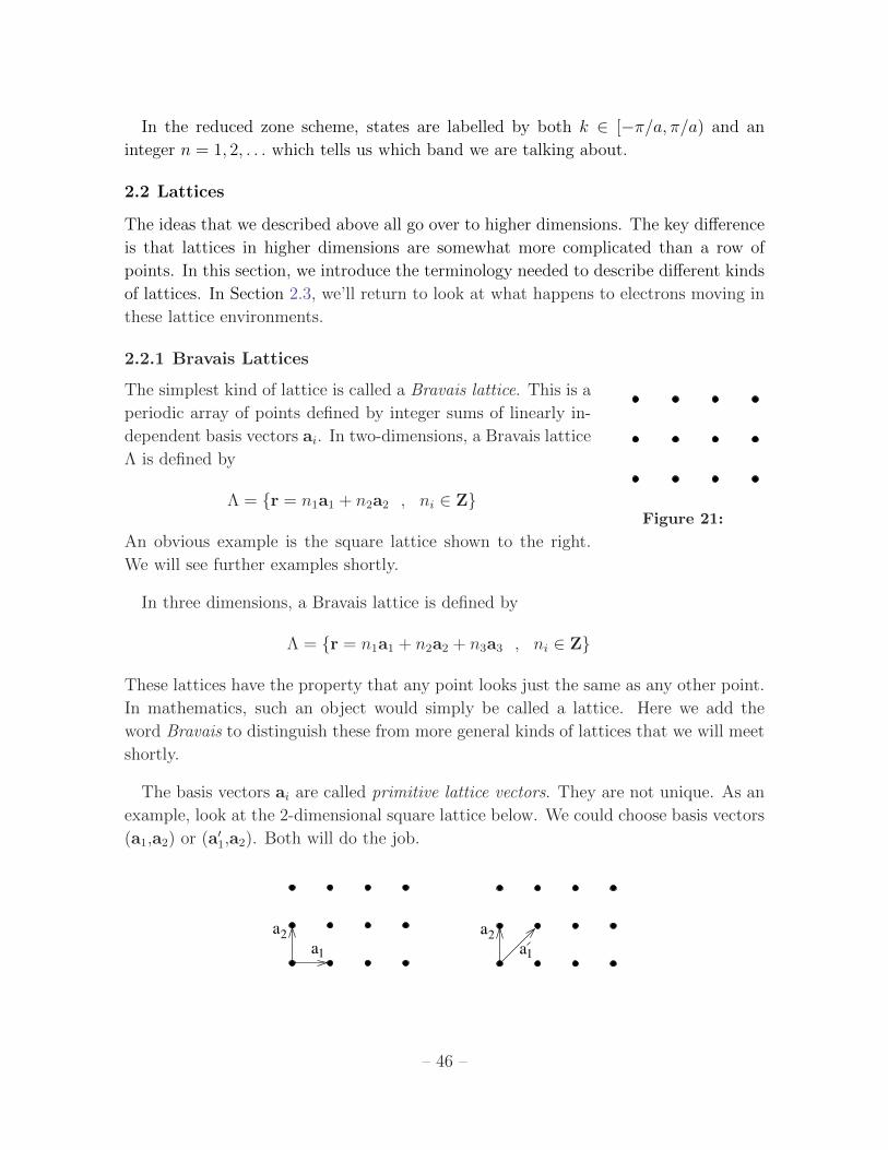
In the reduced zone scheme, states are labelled by both k ∈ [−π/a, π/a) and an

integer n = 1, 2, . . . which tells us which band we are talking about.

2.2 Lattices

The ideas that we described above all go over to higher dimensions. The key difference

is that lattices in higher dimensions are somewhat more complicated than a row of

points. In this section, we introduce the terminology needed to describe different kinds

of lattices. In Section 2.3, we’ll return to look at what happens to electrons moving in

these lattice environments.

2.2.1 Bravais Lattices

The simplest kind of lattice is called a Bravais lattice. This is a

Figure 21:

periodic array of points defined by integer sums of linearly in-

dependent basis vectors ai. In two-dimensions, a Bravais lattice

Λ is defined by

Λ = r = n1a1 + n2a2 , ni ∈ Z

An obvious example is the square lattice shown to the right.

We will see further examples shortly.

In three dimensions, a Bravais lattice is defined by

Λ = r = n1a1 + n2a2 + n3a3 , ni ∈ Z

These lattices have the property that any point looks just the same as any other point.

In mathematics, such an object would simply be called a lattice. Here we add the

word Bravais to distinguish these from more general kinds of lattices that we will meet

shortly.

The basis vectors ai are called primitive lattice vectors. They are not unique. As an

example, look at the 2-dimensional square lattice below. We could choose basis vectors

(a1,a2) or (a′1,a2). Both will do the job.

a2

a1

a2

a1

– 46 –

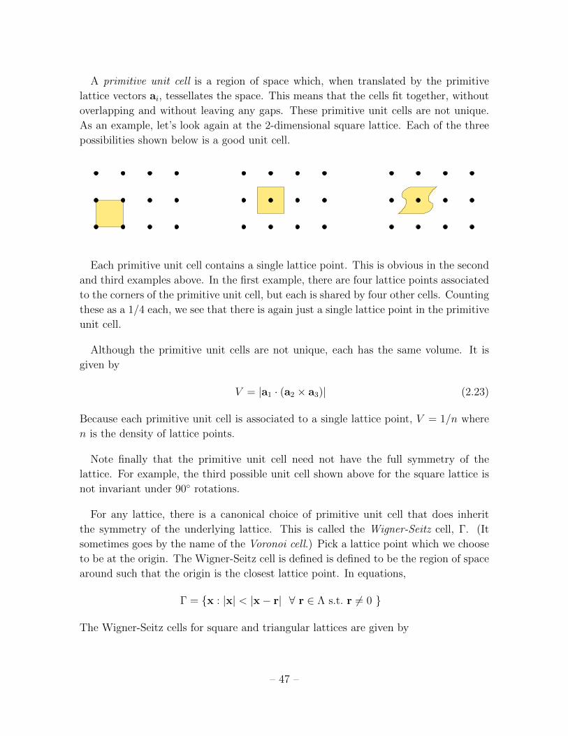
A primitive unit cell is a region of space which, when translated by the primitive

lattice vectors ai, tessellates the space. This means that the cells fit together, without

overlapping and without leaving any gaps. These primitive unit cells are not unique.

As an example, let’s look again at the 2-dimensional square lattice. Each of the three

possibilities shown below is a good unit cell.

Each primitive unit cell contains a single lattice point. This is obvious in the second

and third examples above. In the first example, there are four lattice points associated

to the corners of the primitive unit cell, but each is shared by four other cells. Counting

these as a 1/4 each, we see that there is again just a single lattice point in the primitive

unit cell.

Although the primitive unit cells are not unique, each has the same volume. It is

given by

V = |a1 · (a2 × a3)| (2.23)

Because each primitive unit cell is associated to a single lattice point, V = 1/n where

n is the density of lattice points.

Note finally that the primitive unit cell need not have the full symmetry of the

lattice. For example, the third possible unit cell shown above for the square lattice is

not invariant under 90 rotations.

For any lattice, there is a canonical choice of primitive unit cell that does inherit

the symmetry of the underlying lattice. This is called the Wigner-Seitz cell, Γ. (It

sometimes goes by the name of the Voronoi cell.) Pick a lattice point which we choose

to be at the origin. The Wigner-Seitz cell is defined is defined to be the region of space

around such that the origin is the closest lattice point. In equations,

Γ = x : |x| < |x− r| ∀ r ∈ Λ s.t. r 6= 0

The Wigner-Seitz cells for square and triangular lattices are given by

– 47 –

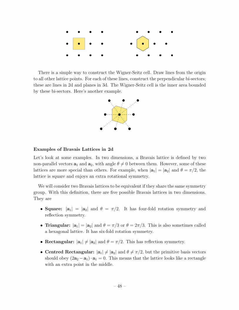
There is a simple way to construct the Wigner-Seitz cell. Draw lines from the origin

to all other lattice points. For each of these lines, construct the perpendicular bi-sectors;

these are lines in 2d and planes in 3d. The Wigner-Seitz cell is the inner area bounded

by these bi-sectors. Here’s another example.

Examples of Bravais Lattices in 2d

Let’s look at some examples. In two dimensions, a Bravais lattice is defined by two

non-parallel vectors a1 and a2, with angle θ 6= 0 between them. However, some of these

lattices are more special than others. For example, when |a1| = |a2| and θ = π/2, the

lattice is square and enjoys an extra rotational symmetry.

We will consider two Bravais lattices to be equivalent if they share the same symmetry

group. With this definition, there are five possible Bravais lattices in two dimensions.

They are

• Square: |a1| = |a2| and θ = π/2. It has four-fold rotation symmetry and

reflection symmetry.

• Triangular: |a1| = |a2| and θ = π/3 or θ = 2π/3. This is also sometimes called

a hexagonal lattice. It has six-fold rotation symmetry.

• Rectangular: |a1| 6= |a2| and θ = π/2. This has reflection symmetry.

• Centred Rectangular: |a1| 6= |a2| and θ 6= π/2, but the primitive basis vectors

should obey (2a2−a1) ·a1 = 0. This means that the lattice looks like a rectangle

with an extra point in the middle.

– 48 –

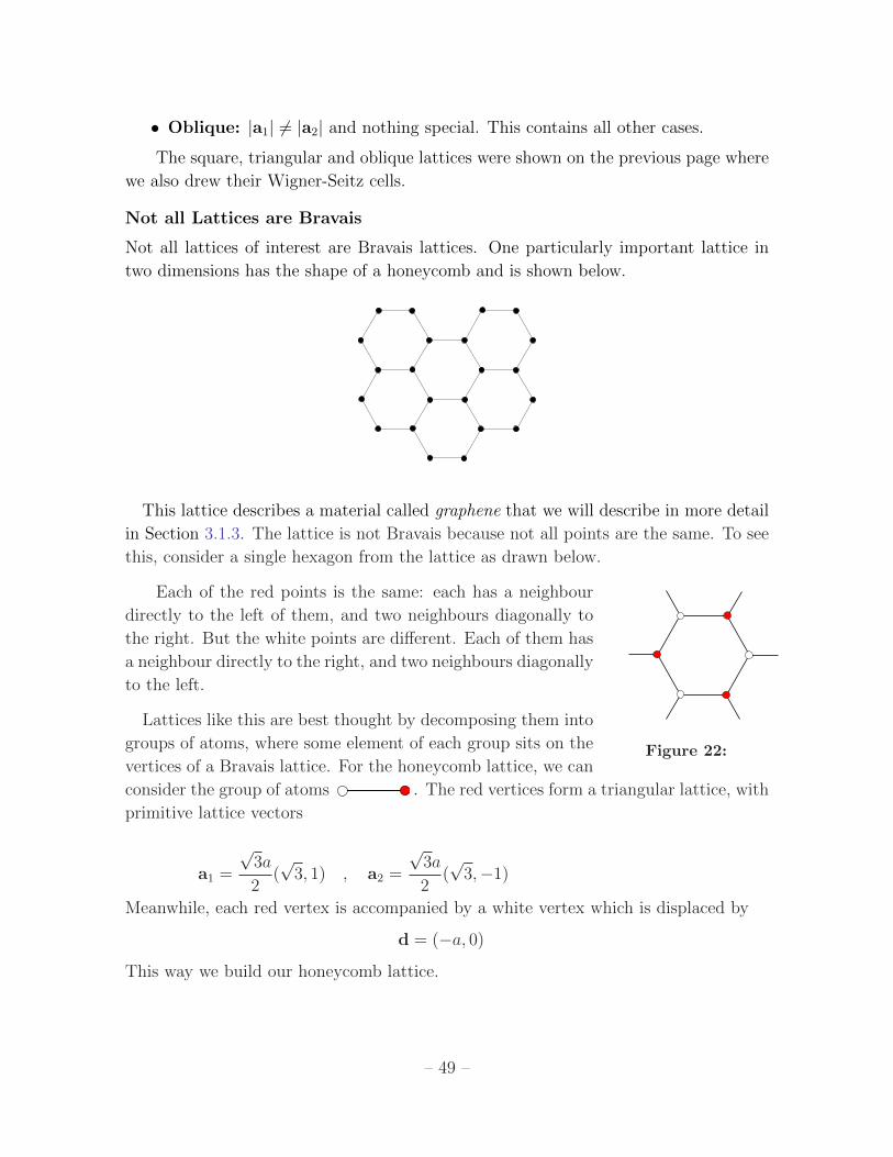
• Oblique: |a1| 6= |a2| and nothing special. This contains all other cases.

The square, triangular and oblique lattices were shown on the previous page where

we also drew their Wigner-Seitz cells.

Not all Lattices are Bravais

Not all lattices of interest are Bravais lattices. One particularly important lattice in

two dimensions has the shape of a honeycomb and is shown below.

This lattice describes a material called graphene that we will describe in more detail

in Section 3.1.3. The lattice is not Bravais because not all points are the same. To see

this, consider a single hexagon from the lattice as drawn below.

Each of the red points is the same: each has a neighbour

Figure 22:

directly to the left of them, and two neighbours diagonally to

the right. But the white points are different. Each of them has

a neighbour directly to the right, and two neighbours diagonally

to the left.

Lattices like this are best thought by decomposing them into

groups of atoms, where some element of each group sits on the

vertices of a Bravais lattice. For the honeycomb lattice, we can

consider the group of atoms . The red vertices form a triangular lattice, with

primitive lattice vectors

a1 =

√3a

2(√

3, 1) , a2 =

√3a

2(√

3,−1)

Meanwhile, each red vertex is accompanied by a white vertex which is displaced by

d = (−a, 0)

This way we build our honeycomb lattice.

– 49 –

This kind of construction generalises. We can describe any

a2

a1

Figure 23:

lattice as a repeating group of atoms, where each group sits on an

underlying Bravais lattice Λ. Each atom in the group is displaced

from the vertex of the Bravais lattice by a vector di. Each group of

atoms, labelled by their positions di is called the basis. For example,

for the honeycomb lattice we chose the basis d1 = 0 for red atoms

and d2 = d for white atoms, since the red atoms sat at the positions

of the underlying triangular lattice. In general there’s no require-

ment that any atom sits on the vertex of the underlying Bravais lattice. The whole

lattice is then described by the union of the Bravais lattice and the basis, ∪iΛ + di.

Examples of Bravais Lattices in 3d

It turns out that there are 14 different Bravais lattices in three dimensions. Fortunately

we won’t need all of them. In fact, we will describe only the three that arise most

frequently in Nature. These are:

• Cubic: This is the simplest lattice. The primitive lattice vectors are aligned with

the Euclidean axes

a1 = ax , a2 = ay , a3 = az

And the primitive cell has volume V = a3. The Wigner-Seitz cell is also a cube,

centered around one of the lattice points.

• Body Centered Cubic (BCC): This is a cubic lattice, with an extra point

placed at the centre of each cube. We could take the primitive lattice vectors to

be

a1 = ax , a2 = ay , a3 =a

2(x + y + z)

However, a more symmetric choice is

a1 =a

2(−x + y + z) , a2 =

a

2(x− y + z) , a3 =

a

2(x + y − z)

The primitive unit cell has volume V = a3/2.

The BCC lattice can also be thought of as a cubic lattice, with a basis of two

atoms with d1 = 0 and d2 = a2(x + y + z). However, this doesn’t affect the fact

that the BCC lattice is itself Bravais.

– 50 –

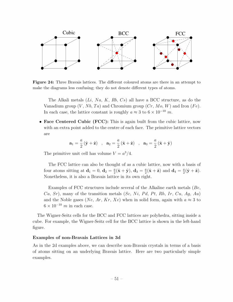
Cubic BCC FCC

Figure 24: Three Bravais lattices. The different coloured atoms are there in an attempt to

make the diagrams less confusing; they do not denote different types of atoms.

The Alkali metals (Li, Na, K, Rb, Cs) all have a BCC structure, as do the

Vanadium group (V , Nb, Ta) and Chromium group (Cr, Mo, W ) and Iron (Fe).

In each case, the lattice constant is roughly a ≈ 3 to 6× 10−10 m.

• Face Centered Cubic (FCC): This is again built from the cubic lattice, now

with an extra point added to the centre of each face. The primitive lattice vectors

are

a1 =a

2(y + z) , a2 =

a

2(x + z) , a3 =

a

2(x + y)

The primitive unit cell has volume V = a3/4.

The FCC lattice can also be thought of as a cubic lattice, now with a basis of

four atoms sitting at d1 = 0, d2 = a2(x + y), d3 = a

2(x + z) and d4 = a

2(y + z).

Nonetheless, it is also a Bravais lattice in its own right.

Examples of FCC structures include several of the Alkaline earth metals (Be,

Ca, Sr), many of the transition metals (Sc, Ni, Pd, Pt, Rh, Ir, Cu, Ag, Au)

and the Noble gases (Ne, Ar, Kr, Xe) when in solid form, again with a ≈ 3 to

6× 10−10 m in each case.

The Wigner-Seitz cells for the BCC and FCC lattices are polyhedra, sitting inside a

cube. For example, the Wigner-Seitz cell for the BCC lattice is shown in the left-hand

figure.

Examples of non-Bravais Lattices in 3d

As in the 2d examples above, we can describe non-Bravais crystals in terms of a basis

of atoms sitting on an underlying Bravais lattice. Here are two particularly simple

examples.

– 51 –

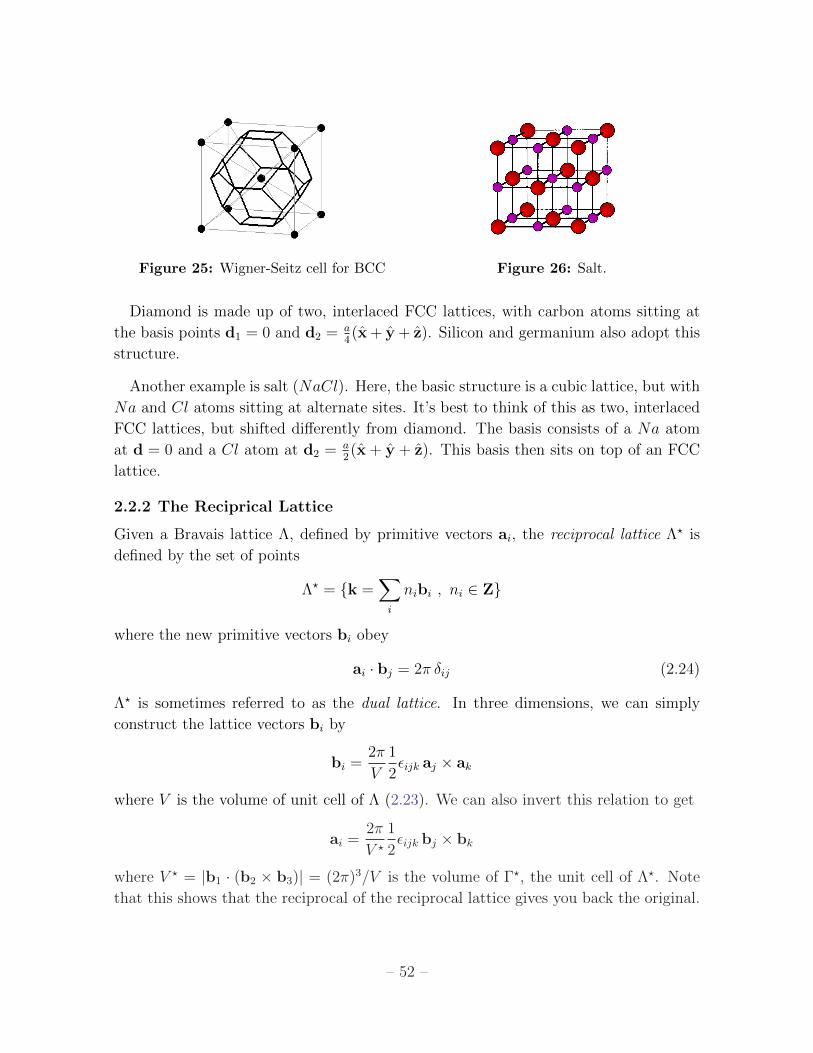
Figure 25: Wigner-Seitz cell for BCC Figure 26: Salt.

Diamond is made up of two, interlaced FCC lattices, with carbon atoms sitting at

the basis points d1 = 0 and d2 = a4(x + y + z). Silicon and germanium also adopt this

structure.

Another example is salt (NaCl). Here, the basic structure is a cubic lattice, but with

Na and Cl atoms sitting at alternate sites. It’s best to think of this as two, interlaced

FCC lattices, but shifted differently from diamond. The basis consists of a Na atom

at d = 0 and a Cl atom at d2 = a2(x + y + z). This basis then sits on top of an FCC

lattice.

2.2.2 The Reciprical Lattice

Given a Bravais lattice Λ, defined by primitive vectors ai, the reciprocal lattice Λ? is

defined by the set of points

Λ? = k =∑i

nibi , ni ∈ Z

where the new primitive vectors bi obey

ai · bj = 2π δij (2.24)

Λ? is sometimes referred to as the dual lattice. In three dimensions, we can simply

construct the lattice vectors bi by

bi =2π

V

1

2εijk aj × ak

where V is the volume of unit cell of Λ (2.23). We can also invert this relation to get

ai =2π

V ?

1

2εijk bj × bk

where V ? = |b1 · (b2 × b3)| = (2π)3/V is the volume of Γ?, the unit cell of Λ?. Note

that this shows that the reciprocal of the reciprocal lattice gives you back the original.

– 52 –

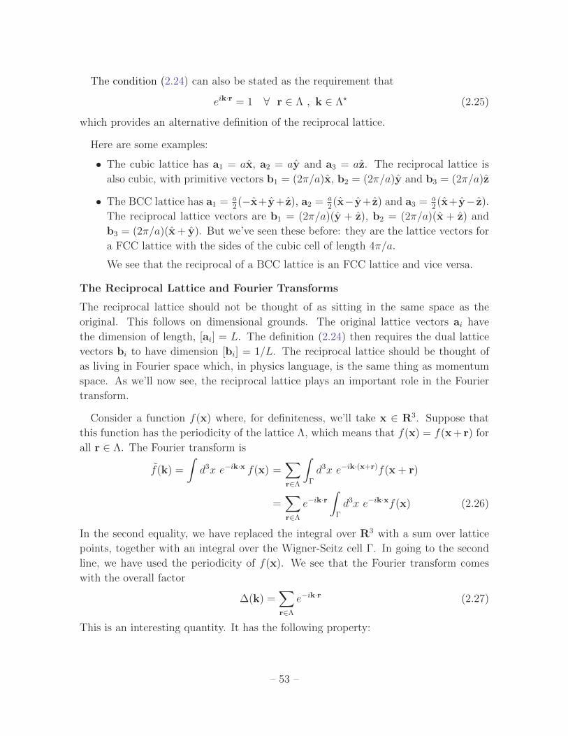
The condition (2.24) can also be stated as the requirement that

eik·r = 1 ∀ r ∈ Λ , k ∈ Λ? (2.25)

which provides an alternative definition of the reciprocal lattice.

Here are some examples:

• The cubic lattice has a1 = ax, a2 = ay and a3 = az. The reciprocal lattice is

also cubic, with primitive vectors b1 = (2π/a)x, b2 = (2π/a)y and b3 = (2π/a)z

• The BCC lattice has a1 = a2(−x+ y+ z), a2 = a

2(x− y+ z) and a3 = a

2(x+ y− z).

The reciprocal lattice vectors are b1 = (2π/a)(y + z), b2 = (2π/a)(x + z) and

b3 = (2π/a)(x + y). But we’ve seen these before: they are the lattice vectors for

a FCC lattice with the sides of the cubic cell of length 4π/a.

We see that the reciprocal of a BCC lattice is an FCC lattice and vice versa.

The Reciprocal Lattice and Fourier Transforms

The reciprocal lattice should not be thought of as sitting in the same space as the

original. This follows on dimensional grounds. The original lattice vectors ai have

the dimension of length, [ai] = L. The definition (2.24) then requires the dual lattice

vectors bi to have dimension [bi] = 1/L. The reciprocal lattice should be thought of

as living in Fourier space which, in physics language, is the same thing as momentum

space. As we’ll now see, the reciprocal lattice plays an important role in the Fourier

transform.

Consider a function f(x) where, for definiteness, we’ll take x ∈ R3. Suppose that

this function has the periodicity of the lattice Λ, which means that f(x) = f(x + r) for

all r ∈ Λ. The Fourier transform is

f(k) =

∫d3x e−ik·x f(x) =

∑r∈Λ

∫Γ

d3x e−ik·(x+r)f(x + r)

=∑r∈Λ

e−ik·r∫

Γ

d3x e−ik·xf(x) (2.26)

In the second equality, we have replaced the integral over R3 with a sum over lattice

points, together with an integral over the Wigner-Seitz cell Γ. In going to the second

line, we have used the periodicity of f(x). We see that the Fourier transform comes

with the overall factor

∆(k) =∑r∈Λ

e−ik·r (2.27)

This is an interesting quantity. It has the following property:

– 53 –

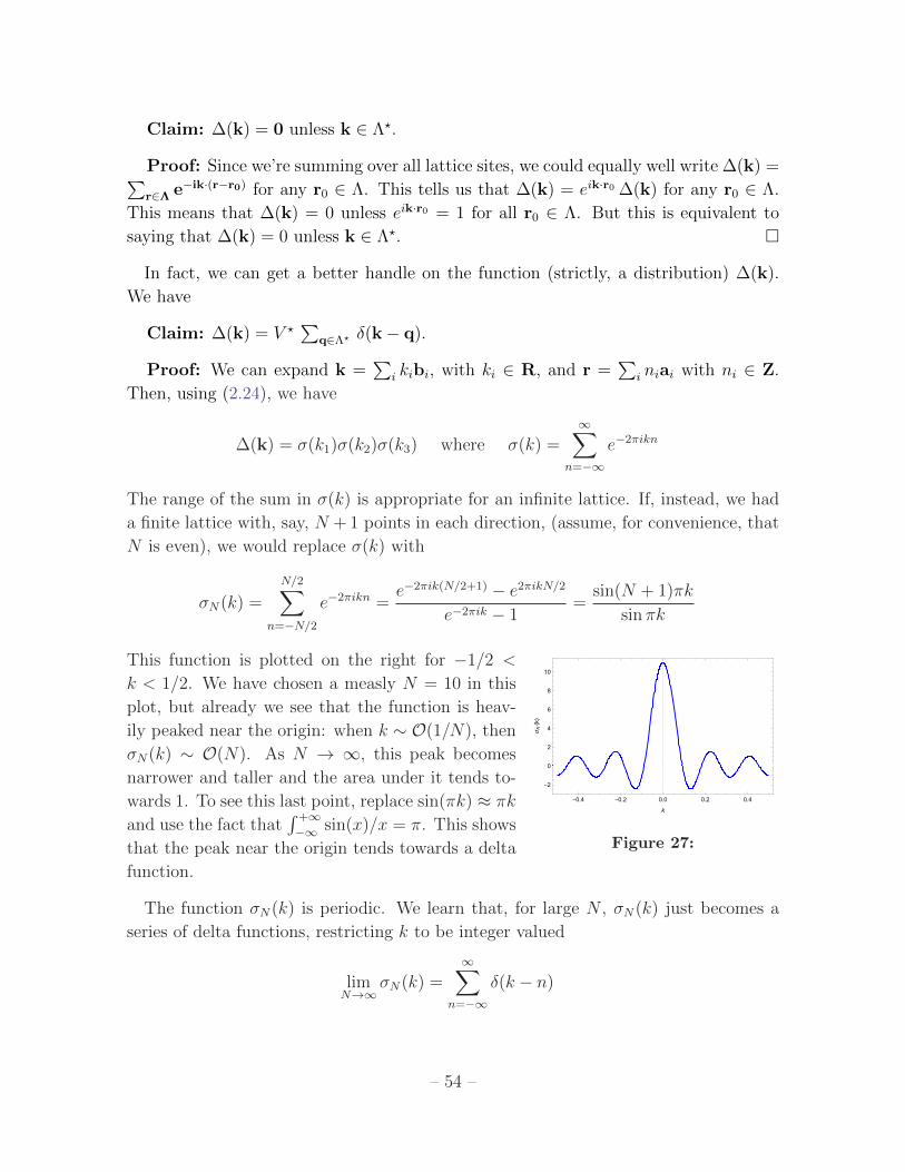
Claim: ∆(k) = 0 unless k ∈ Λ?.

Proof: Since we’re summing over all lattice sites, we could equally well write ∆(k) =∑r∈Λ e−ik·(r−r0) for any r0 ∈ Λ. This tells us that ∆(k) = eik·r0 ∆(k) for any r0 ∈ Λ.

This means that ∆(k) = 0 unless eik·r0 = 1 for all r0 ∈ Λ. But this is equivalent to

saying that ∆(k) = 0 unless k ∈ Λ?.

In fact, we can get a better handle on the function (strictly, a distribution) ∆(k).

We have

Claim: ∆(k) = V ?∑

q∈Λ? δ(k− q).

Proof: We can expand k =∑

i kibi, with ki ∈ R, and r =∑

i niai with ni ∈ Z.

Then, using (2.24), we have

∆(k) = σ(k1)σ(k2)σ(k3) where σ(k) =∞∑

n=−∞

e−2πikn

The range of the sum in σ(k) is appropriate for an infinite lattice. If, instead, we had

a finite lattice with, say, N + 1 points in each direction, (assume, for convenience, that

N is even), we would replace σ(k) with

σN(k) =

N/2∑n=−N/2

e−2πikn =e−2πik(N/2+1) − e2πikN/2

e−2πik − 1=

sin(N + 1)πk

sinπk

This function is plotted on the right for −1/2 <

-0.4 -0.2 0.0 0.2 0.4

-2

0

2

4

6

8

10

k

σN(k)

Figure 27:

k < 1/2. We have chosen a measly N = 10 in this

plot, but already we see that the function is heav-

ily peaked near the origin: when k ∼ O(1/N), then

σN(k) ∼ O(N). As N → ∞, this peak becomes

narrower and taller and the area under it tends to-

wards 1. To see this last point, replace sin(πk) ≈ πk

and use the fact that∫ +∞−∞ sin(x)/x = π. This shows

that the peak near the origin tends towards a delta

function.

The function σN(k) is periodic. We learn that, for large N , σN(k) just becomes a

series of delta functions, restricting k to be integer valued

limN→∞

σN(k) =∞∑

n=−∞

δ(k − n)

– 54 –

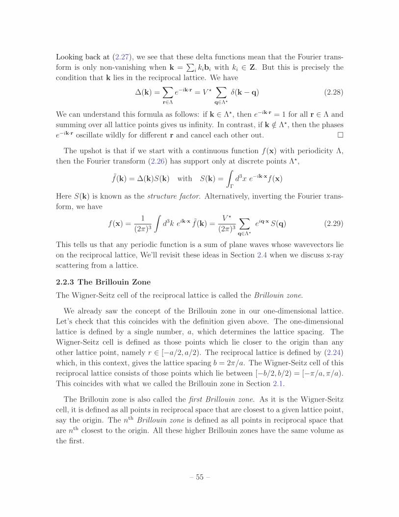
Looking back at (2.27), we see that these delta functions mean that the Fourier trans-

form is only non-vanishing when k =∑

i kibi with ki ∈ Z. But this is precisely the

condition that k lies in the reciprocal lattice. We have

∆(k) =∑r∈Λ

e−ik·r = V ?∑q∈Λ?

δ(k− q) (2.28)

We can understand this formula as follows: if k ∈ Λ?, then e−ik·r = 1 for all r ∈ Λ and

summing over all lattice points gives us infinity. In contrast, if k /∈ Λ?, then the phases

e−ik·r oscillate wildly for different r and cancel each other out.

The upshot is that if we start with a continuous function f(x) with periodicity Λ,

then the Fourier transform (2.26) has support only at discrete points Λ?,

f(k) = ∆(k)S(k) with S(k) =

∫Γ

d3x e−ik·xf(x)

Here S(k) is known as the structure factor. Alternatively, inverting the Fourier trans-

form, we have

f(x) =1

(2π)3

∫d3k eik·x f(k) =

V ?

(2π)3

∑q∈Λ?

eiq·x S(q) (2.29)

This tells us that any periodic function is a sum of plane waves whose wavevectors lie

on the reciprocal lattice, We’ll revisit these ideas in Section 2.4 when we discuss x-ray

scattering from a lattice.

2.2.3 The Brillouin Zone

The Wigner-Seitz cell of the reciprocal lattice is called the Brillouin zone.

We already saw the concept of the Brillouin zone in our one-dimensional lattice.

Let’s check that this coincides with the definition given above. The one-dimensional

lattice is defined by a single number, a, which determines the lattice spacing. The

Wigner-Seitz cell is defined as those points which lie closer to the origin than any

other lattice point, namely r ∈ [−a/2, a/2). The reciprocal lattice is defined by (2.24)

which, in this context, gives the lattice spacing b = 2π/a. The Wigner-Seitz cell of this

reciprocal lattice consists of those points which lie between [−b/2, b/2) = [−π/a, π/a).

This coincides with what we called the Brillouin zone in Section 2.1.

The Brillouin zone is also called the first Brillouin zone. As it is the Wigner-Seitz

cell, it is defined as all points in reciprocal space that are closest to a given lattice point,

say the origin. The nth Brillouin zone is defined as all points in reciprocal space that

are nth closest to the origin. All these higher Brillouin zones have the same volume as

the first.

– 55 –

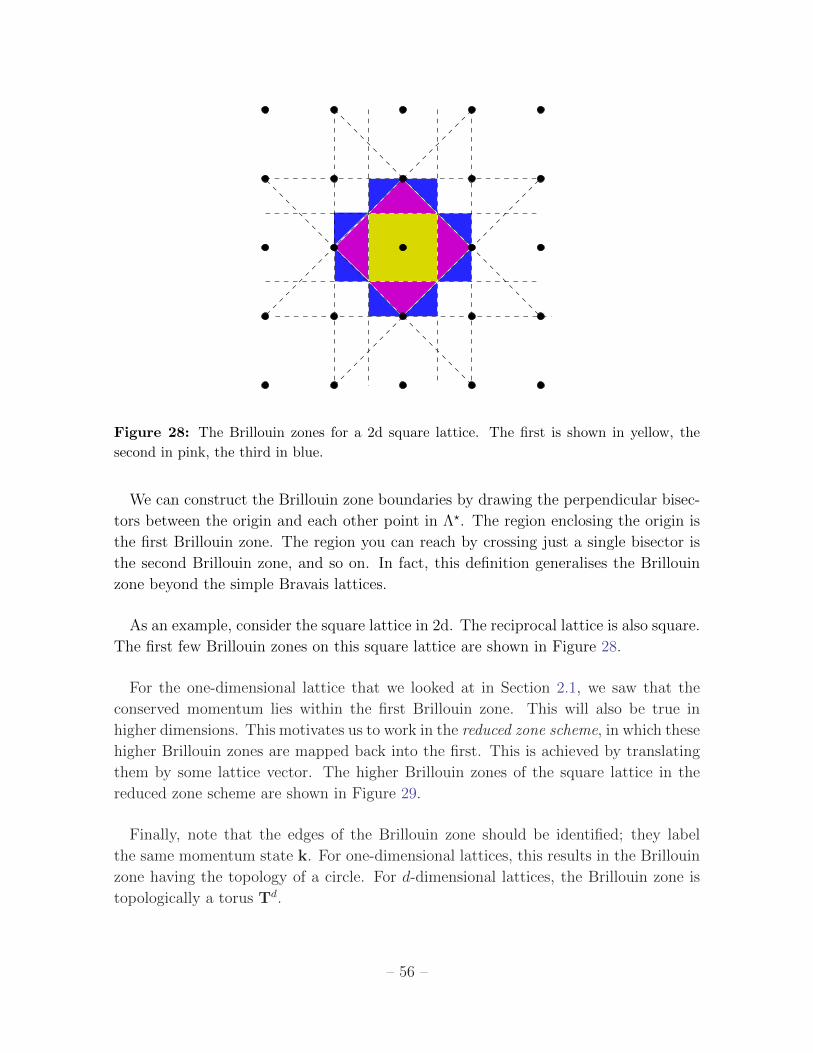
Figure 28: The Brillouin zones for a 2d square lattice. The first is shown in yellow, the

second in pink, the third in blue.

We can construct the Brillouin zone boundaries by drawing the perpendicular bisec-

tors between the origin and each other point in Λ?. The region enclosing the origin is

the first Brillouin zone. The region you can reach by crossing just a single bisector is

the second Brillouin zone, and so on. In fact, this definition generalises the Brillouin

zone beyond the simple Bravais lattices.

As an example, consider the square lattice in 2d. The reciprocal lattice is also square.

The first few Brillouin zones on this square lattice are shown in Figure 28.

For the one-dimensional lattice that we looked at in Section 2.1, we saw that the

conserved momentum lies within the first Brillouin zone. This will also be true in

higher dimensions. This motivates us to work in the reduced zone scheme, in which these

higher Brillouin zones are mapped back into the first. This is achieved by translating

them by some lattice vector. The higher Brillouin zones of the square lattice in the

reduced zone scheme are shown in Figure 29.

Finally, note that the edges of the Brillouin zone should be identified; they label

the same momentum state k. For one-dimensional lattices, this results in the Brillouin

zone having the topology of a circle. For d-dimensional lattices, the Brillouin zone is

topologically a torus Td.

– 56 –

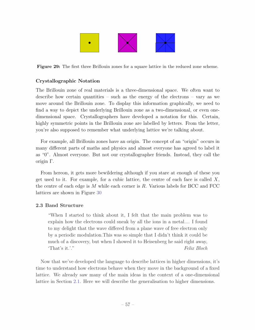
Figure 29: The first three Brillouin zones for a square lattice in the reduced zone scheme.

Crystallographic Notation

The Brillouin zone of real materials is a three-dimensional space. We often want to

describe how certain quantities – such as the energy of the electrons – vary as we

move around the Brillouin zone. To display this information graphically, we need to

find a way to depict the underlying Brillouin zone as a two-dimensional, or even one-

dimensional space. Crystallographers have developed a notation for this. Certain,

highly symmetric points in the Brillouin zone are labelled by letters. From the letter,

you’re also supposed to remember what underlying lattice we’re talking about.

For example, all Brillouin zones have an origin. The concept of an “origin” occurs in

many different parts of maths and physics and almost everyone has agreed to label it

as “0”. Almost everyone. But not our crystallographer friends. Instead, they call the

origin Γ.

From hereon, it gets more bewildering although if you stare at enough of these you

get used to it. For example, for a cubic lattice, the centre of each face is called X,

the centre of each edge is M while each corner is R. Various labels for BCC and FCC

lattices are shown in Figure 30

2.3 Band Structure

“When I started to think about it, I felt that the main problem was to

explain how the electrons could sneak by all the ions in a metal.... I found

to my delight that the wave differed from a plane wave of free electron only

by a periodic modulation.This was so simple that I didn’t think it could be

much of a discovery, but when I showed it to Heisenberg he said right away,

‘That’s it.’.” Felix Bloch

Now that we’ve developed the language to describe lattices in higher dimensions, it’s

time to understand how electrons behave when they move in the background of a fixed

lattice. We already saw many of the main ideas in the context of a one-dimensional

lattice in Section 2.1. Here we will describe the generalisation to higher dimensions.

– 57 –

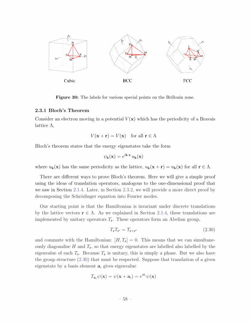
Figure 30: The labels for various special points on the Brillouin zone.

2.3.1 Bloch’s Theorem

Consider an electron moving in a potential V (x) which has the periodicity of a Bravais

lattice Λ,

V (x + r) = V (x) for all r ∈ Λ

Bloch’s theorem states that the energy eigenstates take the form

ψk(x) = eik·x uk(x)

where uk(x) has the same periodicity as the lattice, uk(x + r) = uk(x) for all r ∈ Λ.

There are different ways to prove Bloch’s theorem. Here we will give a simple proof

using the ideas of translation operators, analogous to the one-dimensional proof that

we saw in Section 2.1.4. Later, in Section 2.3.2, we will provide a more direct proof by

decomposing the Schrodinger equation into Fourier modes.

Our starting point is that the Hamiltonian is invariant under discrete translations

by the lattice vectors r ∈ Λ. As we explained in Section 2.1.4, these translations are

implemented by unitary operators Tr. These operators form an Abelian group,

TrTr′ = Tr+r′ (2.30)

and commute with the Hamiltonian: [H,Tr] = 0. This means that we can simultane-

ously diagonalise H and Tr, so that energy eigenstates are labelled also labelled by the

eigenvalue of each Tr. Because Tr is unitary, this is simply a phase. But we also have

the group structure (2.30) that must be respected. Suppose that translation of a given

eigenstate by a basis element ai gives eigenvalue

Taiψ(x) = ψ(x + ai) = eiθiψ(x)

– 58 –

Then translation by a general lattice vector r =∑

i niai must give

Trψ(x) = ψ(x + r) = ei∑

i niθiψ(x) = eik·rψ(x)

where the vector k is defined by k · ai = θi. In other words, we can label eigenstates of

Tr by a vector k. They obey

Trψk(x) = ψk(x + r) = eik·rψk(x)

Now we simply need to look at the function uk(x) = e−ik·xψk(x). The statement

of Bloch’s theorem is that uk(x) has the periodicity of Λ which is indeed true, since

uk(x + r) = e−ik·xe−ik·rψk(x + r) = e−ik·xψk(x) = uk(x).

Crystal Momentum

The energy eigenstates are labelled by the wavevector k, called the crystal momentum.

There is an ambiguity in the definition of this crystal momentum. This is not the same

as the true momentum. The energy eigenstates do not have a well defined momentum

because they are not eigenstates of the momentum operator p = −i~∇ unless uk(x) is

constant. Nonetheless, we will see as we go along that the crystal momentum plays a

role similar to the true momentum. For this reason, we will often refer to k simply as

“momentum”.

There is an ambiguity in the definition of the crystal momentum. Consider a state

with a crystal momentum k′ = k + q, with q ∈ Λ? a reciprocal lattice vector. Then

ψk′(x) = eik·xeiq·xuk(x) = eik·xuk(x)

where uk(x) = eiq·xuk(x) also has the periodicity of Λ by virtue of the definition of the

reciprocal lattice (2.25).

As in the one-dimensional example, we have different options. We could choose to

label states by k which lie in the first Brillouin zone. In this case, there will typically be

many states with the same k and different energies. This is the reduced zone scheme. In

this case, the energy eigenstates are labelled by two indices, ψk,n, where k is the crystal

momentum and n is referred to as the band index. (We will see examples shortly.)

Alternatively, we can label states by taking any k ∈ Rd where d is the dimension of

the problem. This is the extended zone scheme. In this case that states labelled by k

which differ by Λ? have the same crystal momenta.

– 59 –

2.3.2 Nearly Free Electrons in Three Dimensions

Consider an electron moving in R3 in the presence of a weak potential V (x). We’ll

assume that this potential has the periodicity of a Bravais lattice Λ, so

V (x) = V (x + r) for all r ∈ Λ

We treat this potential as a perturbation on the free electron. This means that we start

with plane wave states |k〉 with wavefunctions

〈x|k〉 ∼ eik·x

with energy E0(k) = ~k2/2m. We want to see how these states and their energy levels

are affected by the presence of the potential. The discussion will follow closely the one-

dimensional case that we saw in Section 2.1.2 and we only highlight the differences.

When performing perturbation theory, we’re going to have to consider the potential

V (x) sandwiched between plane-wave states,

〈k|V (x)|k′〉 =1

Volume

∫d3x ei(k

′−k)·x V (x)

However, we’ve already seen in (2.29) that the Fourier transform of a periodic function

can be written as a sum over wavevectors that lie in the reciprocal lattice Λ?,

V (x) =∑q∈Λ?

eiq·x Vq

(Note: here Vq is the Fourier component of the potential and should not be confused

with the volumes of unit cells which were denoted as V and V ? in Section 2.2.) This

means that 〈k|V (x)|k′〉 is non-vanishing only when the two momenta differ by

k− k′ = q q ∈ Λ?

This has a simple physical interpretation: a plane wave state |k〉 can scatter into

another plane wave state |k′〉 only if they differ by a reciprocal lattice vector. In other

words, only momenta q, with q ∈ Λ?, can be absorbed by the lattice.

Another Perspective on Bloch’s Theorem

The fact that that a plane wave state |k〉 can only scatter into states |k− q〉, with q ∈Λ?, provides a simple viewpoint on Bloch’s theorem, one that reconciles the quantum

state with the naive picture of the particle bouncing off lattice sites like a ball in a

pinball machine. Suppose that the particle starts in some state |k〉. After scattering,

– 60 –

we might expect it to be some superposition of all the possible scattering states |k− q〉.In other words,

ψk(x) =∑q∈Λ?

ei(k−q)·x ck−q

for some coefficients ck−q. We can write this as

ψk(x) = eik·x∑q∈Λ?

e−iq·x ck−q = eik·x uk(x)

where, by construction, uk(x + r) = uk(x) for all r ∈ Λ. But this is precisely the form

guaranteed by Bloch’s theorem.

Although the discussion here holds at first order in perturbation theory, it is not

hard to extend this argument to give an alternative proof of Bloch’s theorem, which

essentially comes down to analysing the different Fourier modes of the Schrodinger

equation.

Band Structure

Let’s now look at what becomes of the energy levels after we include the perturbation.

We will see that, as in the 1d example, they form bands. The resulting eigenstates

ψk,n(x) and their associated energy levels En(k) are referred to as the band structure

of the system.

Low Momentum: Far from the edge of the Brillouin zone, the states |k〉 can only

scatter into states |k + q〉 with greatly different energy. In this case, we can work with

non-degenerate perturbation theory to compute the corrections to the energy levels.

On the Boundary of the Brillouin zone: Things get more interesting when we have

to use degenerate perturbation theory. This occurs whenever the state |k〉 has the same

energy as another state |k + q〉 with q ∈ Λ?,

E0(k) = E0(k + q) ⇒ k2 = (k + q)2 ⇒ 2k · q + q2 = 0

This condition is satisfied whenever we can write

k = −1

2q + k⊥

where q · k⊥ = 0. This is the condition that we sit on the perpendicular bisector of

the origin and the lattice point −q ∈ Λ?. But, as we explained in Section 2.2.3, these

bisectors form the boundaries of the Brillouin zones. We learn something important:

momentum states are degenerate only when they lie on the boundary of a Brillouin

zone. This agrees with what we found in our one-dimensional example in Section 2.1.2.

– 61 –

π/a

π/a

−π/a−π/a k

ky

x

Figure 31: Energy contours for nearly-free electrons in the first Brillouin zone.

We know from experience what the effect of the perturbation V (x) will be: it will lift

the degeneracy. This means that a gap opens at the boundary of the Brillouin zone. For

example, the energy of states just inside the first Brillouin zone will be pushed down,

while the energy of those states just outside the first Brillouin zone will be pushed up.

Note that the size of this gap will vary as we move around the boundary..

There is one further subtlety that we should mention. At a generic point on the

boundary of the Brillouin zone, the degeneracy will usually be two-fold. However, at

special points — such as edges, or corners — it is often higher. In this case, we must

work with all degenerate states when computing the gap.

All of this is well illustrated with an example. However, it’s illustrated even better if

you do the example yourself! The problem of nearly free electrons in a two-dimensional

square lattice is on the problem sheet. The resulting energy contours are shown in

Figure 31.

Plotting Band Structures in Three Dimensions

For three-dimensional lattice, we run into the problem of depicting the bands. For this,

we need the crystallographer’s notation we described previously. The spectrum of free

particles (i.e. with no lattice) is plotted in the Brillouin zone of BCC and FCC lattices

in Figure 321.

We can then compare this to the band structure of real materials. The dispersion

relation for silicon is also shown in Figure 32. This has a diamond lattice structure,

which is plotted as FCC. Note that you can clearly see the energy gap of around 1.1 eV

between the bands.1Images plotted by Jan-Rens Reitsma, from Wikimedia commons.

– 62 –

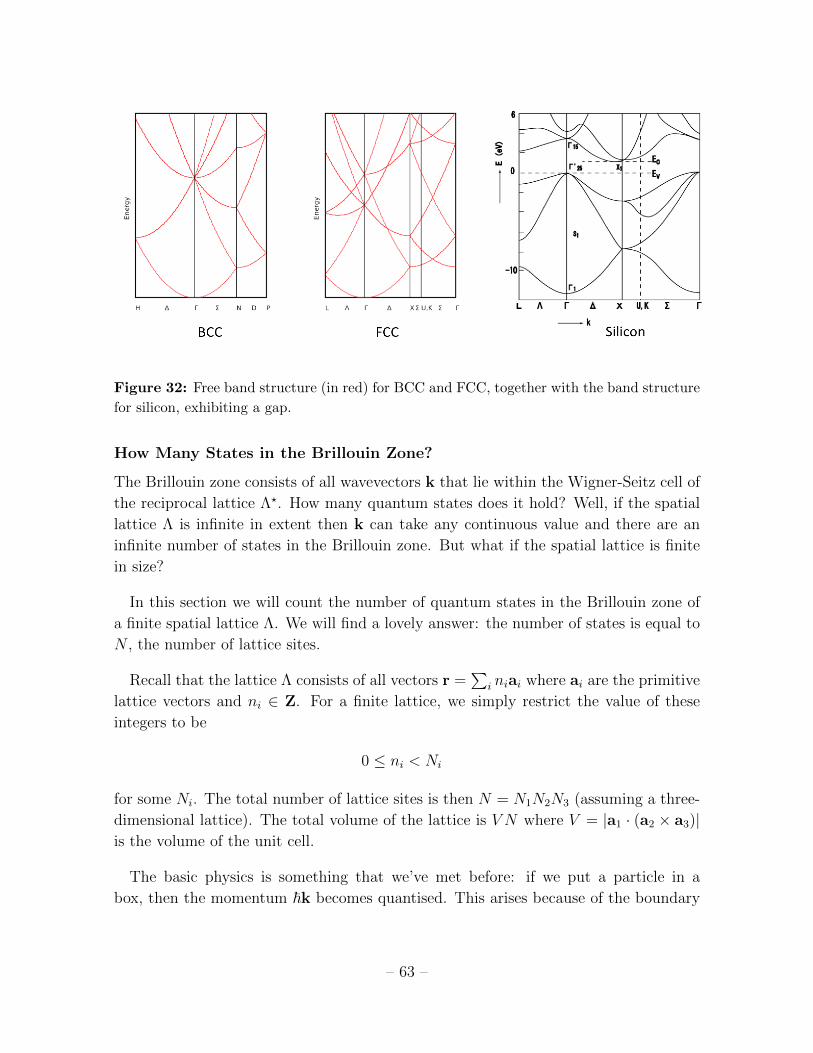
Figure 32: Free band structure (in red) for BCC and FCC, together with the band structure

for silicon, exhibiting a gap.

How Many States in the Brillouin Zone?

The Brillouin zone consists of all wavevectors k that lie within the Wigner-Seitz cell of

the reciprocal lattice Λ?. How many quantum states does it hold? Well, if the spatial

lattice Λ is infinite in extent then k can take any continuous value and there are an

infinite number of states in the Brillouin zone. But what if the spatial lattice is finite

in size?

In this section we will count the number of quantum states in the Brillouin zone of

a finite spatial lattice Λ. We will find a lovely answer: the number of states is equal to

N , the number of lattice sites.

Recall that the lattice Λ consists of all vectors r =∑

i niai where ai are the primitive

lattice vectors and ni ∈ Z. For a finite lattice, we simply restrict the value of these

integers to be

0 ≤ ni < Ni

for some Ni. The total number of lattice sites is then N = N1N2N3 (assuming a three-

dimensional lattice). The total volume of the lattice is V N where V = |a1 · (a2 × a3)|is the volume of the unit cell.

The basic physics is something that we’ve met before: if we put a particle in a

box, then the momentum ~k becomes quantised. This arises because of the boundary

– 63 –

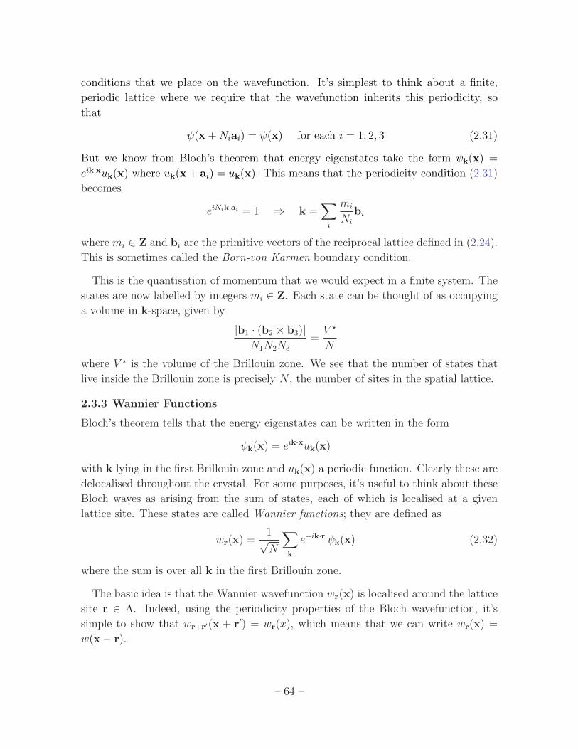
conditions that we place on the wavefunction. It’s simplest to think about a finite,

periodic lattice where we require that the wavefunction inherits this periodicity, so

that

ψ(x +Niai) = ψ(x) for each i = 1, 2, 3 (2.31)

But we know from Bloch’s theorem that energy eigenstates take the form ψk(x) =

eik·xuk(x) where uk(x + ai) = uk(x). This means that the periodicity condition (2.31)

becomes

eiNik·ai = 1 ⇒ k =∑i

mi

Ni

bi

where mi ∈ Z and bi are the primitive vectors of the reciprocal lattice defined in (2.24).

This is sometimes called the Born-von Karmen boundary condition.

This is the quantisation of momentum that we would expect in a finite system. The

states are now labelled by integers mi ∈ Z. Each state can be thought of as occupying

a volume in k-space, given by

|b1 · (b2 × b3)|N1N2N3

=V ?

N

where V ? is the volume of the Brillouin zone. We see that the number of states that

live inside the Brillouin zone is precisely N , the number of sites in the spatial lattice.

2.3.3 Wannier Functions

Bloch’s theorem tells that the energy eigenstates can be written in the form

ψk(x) = eik·xuk(x)

with k lying in the first Brillouin zone and uk(x) a periodic function. Clearly these are

delocalised throughout the crystal. For some purposes, it’s useful to think about these

Bloch waves as arising from the sum of states, each of which is localised at a given

lattice site. These states are called Wannier functions; they are defined as

wr(x) =1√N

∑k

e−ik·r ψk(x) (2.32)

where the sum is over all k in the first Brillouin zone.

The basic idea is that the Wannier wavefunction wr(x) is localised around the lattice

site r ∈ Λ. Indeed, using the periodicity properties of the Bloch wavefunction, it’s

simple to show that wr+r′(x + r′) = wr(x), which means that we can write wr(x) =

w(x− r).

– 64 –

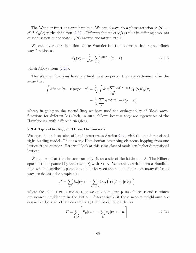
The Wannier functions aren’t unique. We can always do a phase rotation ψk(x) →eiχ(k)ψk(k) in the definition (2.32). Different choices of χ(k) result in differing amounts

of localisation of the state wr(x) around the lattice site r.

We can invert the definition of the Wannier function to write the original Bloch

wavefunction as

ψk(x) =1√N

∑r∈Λ

eik·rw(x− r) (2.33)

which follows from (2.28).

The Wannier functions have one final, nice property: they are orthonormal in the

sense that ∫d3x w?(x− r′)w(x− r) =

1

N

∫d3x

∑k,k′

eik′·r′−ik·rψ?k′(x)ψk(x)

=1

N

∑k

eik·(r′−r) = δ(r− r′)

where, in going to the second line, we have used the orthogonality of Bloch wave-

functions for different k (which, in turn, follows because they are eigenstates of the

Hamiltonian with different energies).

2.3.4 Tight-Binding in Three Dimensions

We started our discussion of band structure in Section 2.1.1 with the one-dimensional

tight binding model. This is a toy Hamiltonian describing electrons hopping from one

lattice site to another. Here we’ll look at this same class of models in higher dimensional

lattices.

We assume that the electron can only sit on a site of the lattice r ∈ Λ. The Hilbert

space is then spanned by the states |r〉 with r ∈ Λ. We want to write down a Hamilto-

nian which describes a particle hopping between these sites. There are many different

ways to do this; the simplest is

H =∑r∈Λ

E0|r〉〈r| −∑<rr′>

tr′−r

(|r〉〈r′|+ |r′〉〈r|

)where the label < rr′ > means that we only sum over pairs of sites r and r′ which

are nearest neighbours in the lattice. Alternatively, if these nearest neighbours are

connected by a set of lattice vectors a, then we can write this as

H =∑r∈Λ

[E0|r〉〈r| −

∑a

ta |r〉〈r + a|

](2.34)

– 65 –

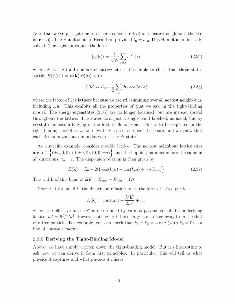
Note that we’ve just got one term here, since if |r + a〉 is a nearest neighbour, then so

is |r− a〉. The Hamiltonian is Hermitian provided ta = t−a This Hamiltonian is easily

solved. The eigenstates take the form

|ψ(k)〉 =1√N

∑r∈Λ

eik·r|r〉 (2.35)

where N is the total number of lattice sites. It’s simple to check that these states

satisfy H|ψ(k)〉 = E(k)|ψ(k)〉 with

E(k) = E0 −1

2

∑a

2ta cos(k · a) (2.36)

where the factor of 1/2 is there because we are still summing over all nearest neighbours,

including ±a. This exhibits all the properties of that we saw in the tight-binding

model. The energy eigenstates (2.35) are no longer localised, but are instead spread

throughout the lattice. The states form just a single band labelled, as usual, but by

crystal momentum k lying in the first Brillouin zone. This is to be expected in the

tight-binding model as we start with N states, one per lattice site, and we know that

each Brillouin zone accommodates precisely N states.

As a specific example, consider a cubic lattice. The nearest neighbour lattice sites

are a ∈

(±a, 0, 0), (0,±a, 0), (0, 0,±a)

and the hopping parameters are the same in

all directions: ta = t. The dispersion relation is then given by

E(k) = E0 − 2t(

cos(kxa) + cos(kya) + cos(kza))

(2.37)

The width of this band is ∆E = Emax − Emin = 12t.

Note that for small k, the dispersion relation takes the form of a free particle

E(k) = constant +~2k2

2m?+ . . .

where the effective mass m? is determined by various parameters of the underlying

lattice, m? = ~2/2ta2. However, at higher k the energy is distorted away from the that

of a free particle. For example, you can check that kx ± ky = ∓π/a (with kz = 0) is a

line of constant energy.

2.3.5 Deriving the Tight-Binding Model

Above, we have simply written down the tight-binding model. But it’s interesting to

ask how we can derive it from first principles. In particular, this will tell us what

physics it captures and what physics it misses.

– 66 –

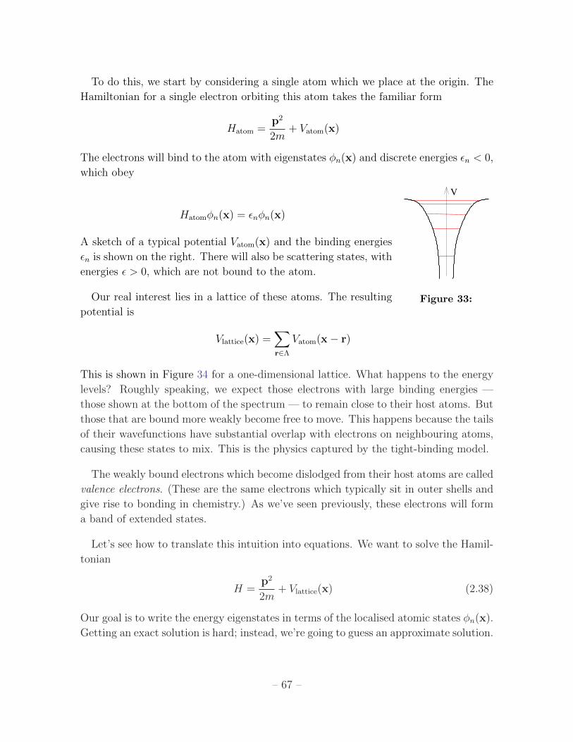
To do this, we start by considering a single atom which we place at the origin. The

Hamiltonian for a single electron orbiting this atom takes the familiar form

Hatom =p2

2m+ Vatom(x)

The electrons will bind to the atom with eigenstates φn(x) and discrete energies εn < 0,

which obey

V

Figure 33:

Hatomφn(x) = εnφn(x)

A sketch of a typical potential Vatom(x) and the binding energies

εn is shown on the right. There will also be scattering states, with

energies ε > 0, which are not bound to the atom.

Our real interest lies in a lattice of these atoms. The resulting

potential is

Vlattice(x) =∑r∈Λ

Vatom(x− r)

This is shown in Figure 34 for a one-dimensional lattice. What happens to the energy

levels? Roughly speaking, we expect those electrons with large binding energies —

those shown at the bottom of the spectrum — to remain close to their host atoms. But

those that are bound more weakly become free to move. This happens because the tails

of their wavefunctions have substantial overlap with electrons on neighbouring atoms,

causing these states to mix. This is the physics captured by the tight-binding model.

The weakly bound electrons which become dislodged from their host atoms are called

valence electrons. (These are the same electrons which typically sit in outer shells and

give rise to bonding in chemistry.) As we’ve seen previously, these electrons will form

a band of extended states.

Let’s see how to translate this intuition into equations. We want to solve the Hamil-

tonian

H =p2

2m+ Vlattice(x) (2.38)

Our goal is to write the energy eigenstates in terms of the localised atomic states φn(x).

Getting an exact solution is hard; instead, we’re going to guess an approximate solution.

– 67 –

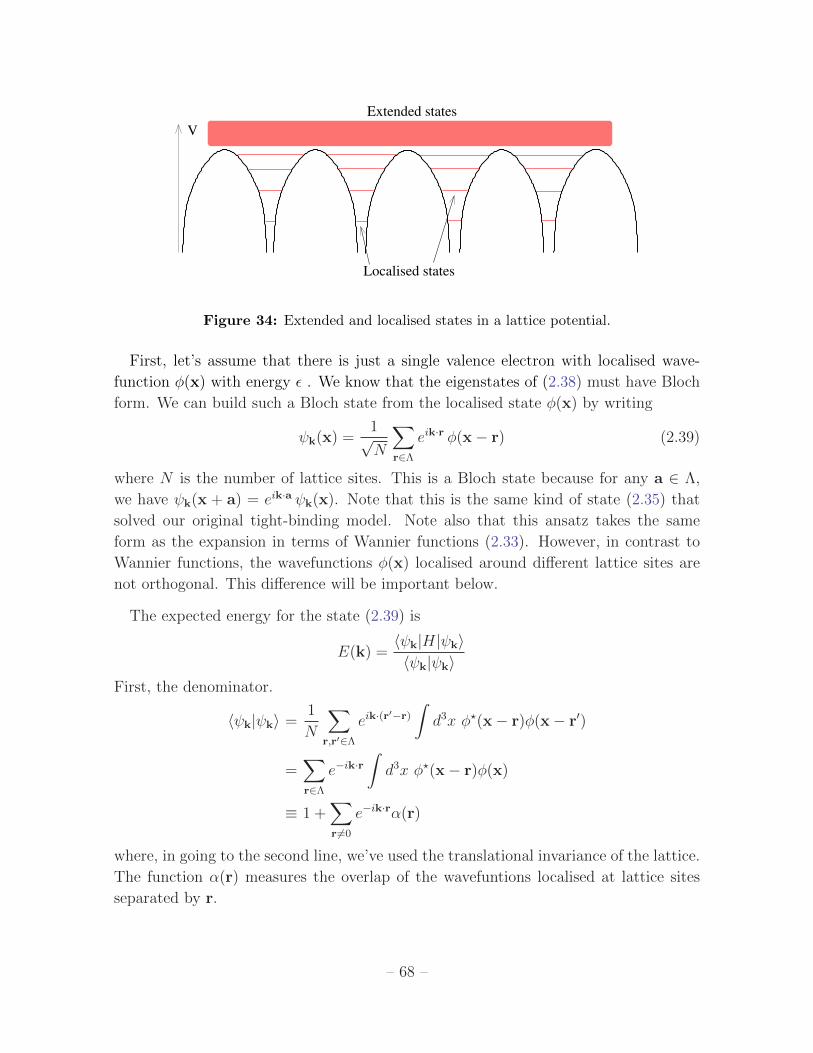
V

Extended states

Localised states

Figure 34: Extended and localised states in a lattice potential.

First, let’s assume that there is just a single valence electron with localised wave-

function φ(x) with energy ε . We know that the eigenstates of (2.38) must have Bloch

form. We can build such a Bloch state from the localised state φ(x) by writing

ψk(x) =1√N

∑r∈Λ

eik·r φ(x− r) (2.39)

where N is the number of lattice sites. This is a Bloch state because for any a ∈ Λ,

we have ψk(x + a) = eik·a ψk(x). Note that this is the same kind of state (2.35) that

solved our original tight-binding model. Note also that this ansatz takes the same

form as the expansion in terms of Wannier functions (2.33). However, in contrast to

Wannier functions, the wavefunctions φ(x) localised around different lattice sites are

not orthogonal. This difference will be important below.

The expected energy for the state (2.39) is

E(k) =〈ψk|H|ψk〉〈ψk|ψk〉

First, the denominator.

〈ψk|ψk〉 =1

N

∑r,r′∈Λ

eik·(r′−r)

∫d3x φ?(x− r)φ(x− r′)

=∑r∈Λ

e−ik·r∫d3x φ?(x− r)φ(x)

≡ 1 +∑r6=0

e−ik·rα(r)

where, in going to the second line, we’ve used the translational invariance of the lattice.

The function α(r) measures the overlap of the wavefuntions localised at lattice sites

separated by r.

– 68 –

Next the numerator. To compute this, we write H = Hatom + ∆V (x) where

∆V (x) = Vlattice(x)− Vatom(x) =∑

r∈Λ,r6=0

Vatom(x− r)

We then have

〈ψk|H|ψk〉 =1

N

∑r,r′∈Λ

eik·(r′−r)

∫d3x φ?(x− r)(Hatom + ∆V )φ(x− r′)

=∑r∈Λ

e−ik·r∫d3x φ?(x− r)(Hatom + ∆V )φ(x)

≡ ε〈ψk|ψk〉+ ∆ε+∑r6=0

e−ik·rγ(r)

Here ∆ε is the shift in the energy of the bound state φ(x) due to the potential ∆V ,

∆ε =

∫d3x φ?(x)∆V (x)φ(x)

Meanwhile, the last term arises from the overlap of localised atoms on different sites

γ(r) =

∫d3x φ?(x− r) ∆V (x)φ(x)

The upshot of this is an expression for the expected energy of the Bloch wave (2.39)

E(k) = ε+∆ε+

∑r6=0 e

−ik·r γ(r)

1 +∑

r6=0 e−ik·r α(r)

Under the assumption that α(r) 1, we can expand out the denominator (1 + x)−1 ≈1− x, and write

E(k) = ε+ ∆ε+∑r6=0

e−ik·r(γ(r)− α(r) ∆ε

)(2.40)

This still looks rather complicated. However, the expression simplifies because the

overlap functions α(r) and γ(r) both drop off quickly with separation. Very often, it’s

sufficient to take these to be non-zero only when r are the nearest neighbour lattice

sites. Sometimes we need to go to next-to-nearest neighbours.

An Example: s-Orbitals

Let’s assume that α(r) and γ(r) are important only for r connecting nearest neighbour

lattice sites; all others will be taken to vanish. We’ll further take the valence electron

– 69 –

to sit in the s-orbital. This has two consequences: first, the localised wavefunction is

rotationally invariant, so that φ(r) = φ(r). Second, the wavefunction can be taken to

be real, so φ?(x) = φ(x). With these restrictions, we have

α(r) =

∫d3xφ(x− r)φ(x) = α(−r)

We want a similar expression for γ(r). For this, we need to make one further assump-

tion: we want the crystal to have inversion symmetry. This means that V (x) = V (−x)

or, more pertinently for us, ∆V (x) = ∆V (−x). We can then write

γ(r) =

∫d3x φ(x− r)∆V (x)φ(x)

=

∫d3x′ φ(−x′ − r)∆V (−x′)φ(−x′)

=

∫d3x′φ(|x′ + r|)∆V (x′)φ(|x′|)

= γ(−r)

where we have defined x′ = −x in the second line and used both the inversion symmetry

and rotational invariance of the s-orbital in the third. Now we can write the energy

(2.40) in a slightly nicer form. We need to remember that the vectors r span a lattice

which ensures that if r is a nearest neighbour site then −r is too. We then have

E(k) = ε+ ∆ε+∑

a

cos(k · a)(γ(a)−∆ε α(a)

)(2.41)

where a are the nearest neighbour lattice sites. We recognise this as the dispersion

relation that we found in our original tight-binding model (2.36), with E0 = ε+∆ε and

ta = γ(a)−∆ε α(a).

So far we’ve shown that the state (2.39) has the same energy as eigenstates of the

tight-binding Hamiltonian. But we haven’t yet understood when the state (2.39) is a

good approximation to the true eigenstate of the Hamiltonian (2.38).

We can intuit the answer to this question by looking in more detail at (2.41). We

see that the localised eigenstates φ(x), each of which had energy ε, have spread into a

band with energies E(k). For this calculation to be valid, it’s important that this band

doesn’t mix with other states. This means that the energies E(k) shouldn’t be too

low, so that it has overlap with the energies of more deeply bound states. Nor should

E(k) be too high, so that it overlaps with the energies of the scattering states which

will give rise to higher bands. If the various lattice parameters are chosen so that it

– 70 –

sits between these two values, our ansatz (2.39) will be a good approximation to the

true wavefunction. Another way of saying this is that if we focus on states in the first

band, we can approximate the Hamiltonian (2.38) describing a lattice of atoms by the

tight-binding Hamiltonian (2.34).

A Linear Combination of Atomic Orbitals

What should we do if the band of interest does overlap with bands from more deeply

bound states? The answer is that we should go back to our original ansatz (2.39) and

replace it with something more general, namely

ψk(x) =1√N

∑r∈Λ

eik·r∑n

cnφn(x− r) (2.42)

where this time we sum over all localised states of interest, φn(x) with energies εn.

These are now weighted with coefficients cn which we will determine shortly. This kind

of ansatz is known as a linear combination of atomic orbitals. Among people who play

these kind of games, it is common enough to have its own acronym (LCAO obviously).

The wavefunction (2.42) should be viewed as a variational ansatz for the eigenstates,

where we get to vary the parameters cn. The expected energy is again

E(k) =〈ψk|H|ψk〉〈ψk|ψk〉

where, repeating the calculations that we just saw, we have

〈ψk|ψk〉 =∑r∈Λ

∑n,n′

c?n′cn e−ik·r

∫d3x φ?n′(x− r)φn(x)

≡∑r∈Λ

∑n,n′

c?n′cn e−ik·rαn,n′(r) (2.43)

and

〈ψk|H|ψk〉 =∑r∈Λ

∑n,n′

c?n′cn e−ik·r

∫d3x φ?n′(x− r)(Hatom + ∆V )φn(x)

≡∑r∈Λ

∑n,n′

c?n′cn e−ik·r

(εnαn,n′(r) + γn,n′(r)

)(2.44)

Note that we’ve used slightly different notation from before. We haven’t isolated the

piece αn,n′(r = 0) = δn,n′ , nor the analogous ∆ε piece corresponding to γn,n′(r = 0).

Instead, we continue to sum over all lattice points r ∈ Λ, including the origin.

– 71 –

The variational principle says that we should minimise the expected energy over all

cn. This means we should solve

∂E(k)

∂c?n′=

1

〈ψk|ψk〉∂

∂c?n′〈ψk|H|ψk〉 −

〈ψk|H|ψk〉〈ψk|ψk〉2

∂

∂c?n′〈ψk|ψk〉 = 0

⇒ ∂

∂c?n′〈ψk|H|ψk〉 − E(k)

∂

∂c?n′〈ψk|ψk〉 = 0

Using our expressions (2.43) and (2.44), we can write the resulting expression as the

matrix equation ∑n

Mn,n′(k)cn = 0 (2.45)

where Mn,n′(k) is the Hermitian matrix

Mn,n′(k) =∑r∈Λ

e−ik·r(γn,n′(r)− (E(k)− εn)αn,n′(r)

)The requirement (2.45) that Mn,n′(k) has a zero eigenvalue can be equivalently written

as

det Mn,n′(k) = 0

Let’s think about how to view this equation. The matrix Mn,n′(k) is a function of

the various parameters which encode the underlying lattice dynamics as well as E(k).

But what we want to figure out is the dispersion relation E(k). We should view the

condition det Mn,n′(k) = 0 as an equation for E(k).

Suppose that we include p localised states at each site, so Mn,n′(k) is a p× p matrix.

Then det Mn,n′(k) = 0 is a polynomial in E(k) of degree p. This polynomial will have

p roots; these are the energies En(k) of p bands. In each case, the corresponding null

eigenvector is cn which tells us how the atomic orbitals mix in the Bloch state (2.42).

2.4 Scattering Off a Lattice

Finally, we come to an important question: how do we know that solids are made of

lattices? The answer, of course, is scattering. Firing a beam of particles — whether

neutrons, electrons or photons in the X-ray spectrum — at the solid reveals a char-

acteristic diffraction pattern. Our goal here is to understand this within the general

context of scattering theory.

In what follows, we will assume a knowledge of the basics of scattering theory. Full

details can be found in the lectures on Topics in Quantum Mechanics.

– 72 –

Our starting point is the standard asymptotic expression describing a wave scattering

off a central potential, localised around the origin,

ψ(r) ∼ eik·r + f(k; k′)eikr

r(2.46)

Here we’re using the notation, introduced in earlier sections, of the scattered momentum

k′ = kr

The idea here is that if you sit far away in the direction r, you will effectively see a wave

with momentum k′. We therefore write f(k,k′) to mean the same thing as f(k; θ, φ).

Suppose now that the wave scatters off a potential which is localised at some other

position, r = R. Then the equation (2.46) becomes

ψ(r) ∼ eik·(r−R) + f(k,k′)eik|r−R|

|r−R|

For r →∞, we can expand

|r−R| =√r2 +R2 − 2r ·R ≈ r

√1− 2r ·R/r2 ≈ r − r ·R

We then have

ψ(r) ∼ e−ik·R[eik·r + f(k,k′)e−i(k

′−k)·R eikr

r

](2.47)

The overall factor is unimportant, since our interest lies in the phase shift between

the incident wave and the scattered wave. We see that we get an effective scattering

amplitude

fR(k; r) = f(k,k′) eiq·R

where we have defined the transferred momentum

q = k− k′

Now let’s turn to a lattice of points Λ. Ignoring multiple scatterings, the amplitude is

simply the sum of the amplitudes from each lattice point

fΛ(k,k′) = f(k,k′)∑R∈Λ

eiq·R (2.48)

– 73 –

However, we already discussed the sum ∆(q) =∑

R∈Λ eiq·R in Section 2.2.2. The sum

has the nice property that it vanishes unless q lies in the reciprocal lattice Λ?. This

is simple to see: since we have an infinite lattice it must be true that, for any vector

R0 ∈ Λ,

∆(q) ≡∑R∈Λ

eiq·R =∑R∈Λ

eiq·(R−R0) = e−iq·R0∆(q)

This means that either e−iq·R0 = 1 or ∆(q) = 0. The former result is equivalent to the

statement that q ∈ Λ?. More generally,∑R∈Λ

eiq·R ≡ ∆(q) = V ?∑

Q∈Λ?

δ(q−Q) (2.49)

where V ? is the volume of the unit cell of Λ?. We see that ∆(q) is very strongly

(formally, infinitely) peaked on the reciprocal lattice.

The upshot of this discussion is a lovely result: there is scattering from a lattice if

and only if

k− k′ ∈ Λ? (2.50)

This is known as the Laue condition. If the scattered momentum does not satisfy

this condition, then the interference between all the different scattering sites results

in a vanishing wave. Only when the Laue condition is obeyed is this interference

constructive.

Alternatively, the Laue condition can be viewed as momentum conservation, with

the intuition — garnered from Section 2 — that the lattice can only absorb momentum

in Λ?.

Solutions to the Laue condition are not generic. If you take a lattice with a fixed

orientation and fire a beam with fixed k, chances are that there are no solutions to

(2.50). To see this, consider the reciprocal lattice as shown in the left-hand panel of

the figure. From the tip of k draw a sphere of radius k. This is sometimes known as

the Ewald sphere and its surface gives the possible transferred momenta q = k − k′.

There is scattering only if this surface passes through a point on the reciprocal lattice.

To get scattering, we must therefore either find a wave to vary the incoming momen-

tum k, or find a way to vary the orientation of the lattice. But when this is achieved,

the outgoing photons k′ = kr sit only at very specific positions. In this way, we get to

literally take a photograph of the reciprocal lattice! The resulting diffraction pattern

for salt (NaCl) which has a cubic lattice structure is shown in the right-hand panel.

The four-fold symmetry of the reciprocal lattice is clearly visible.

– 74 –

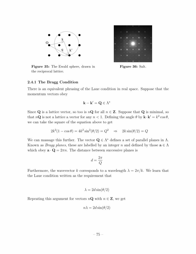
k

k’q

O

Figure 35: The Ewald sphere, drawn in

the reciprocal lattice.

Figure 36: Salt.

2.4.1 The Bragg Condition

There is an equivalent phrasing of the Laue condition in real space. Suppose that the

momentum vectors obey

k− k′ = Q ∈ Λ?

Since Q is a lattice vector, so too is nQ for all n ∈ Z. Suppose that Q is minimal, so

that nQ is not a lattice a vector for any n < 1. Defining the angle θ by k ·k′ = k2 cos θ,

we can take the square of the equation above to get

2k2(1− cos θ) = 4k2 sin2(θ/2) = Q2 ⇒ 2k sin(θ/2) = Q

We can massage this further. The vector Q ∈ Λ? defines a set of parallel planes in Λ.

Known as Bragg planes, these are labelled by an integer n and defined by those a ∈ Λ

which obey a ·Q = 2πn. The distance between successive planes is

d =2π

Q

Furthermore, the wavevector k corresponds to a wavelength λ = 2π/k. We learn that

the Laue condition written as the requirement that

λ = 2d sin(θ/2)

Repeating this argument for vectors nQ with n ∈ Z, we get

nλ = 2d sin(θ/2)

– 75 –

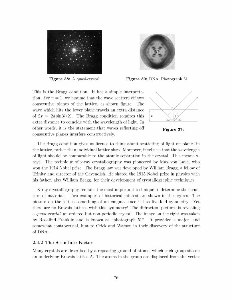
Figure 38: A quasi-crystal. Figure 39: DNA, Photograph 51.

This is the Bragg condition. It has a simple interpreta-

d x

θ/2 θ/2

Figure 37:

tion. For n = 1, we assume that the wave scatters off two

consecutive planes of the lattice, as shown figure. The

wave which hits the lower plane travels an extra distance

of 2x = 2d sin(θ/2). The Bragg condition requires this

extra distance to coincide with the wavelength of light. In

other words, it is the statement that waves reflecting off

consecutive planes interfere constructively.

The Bragg condition gives us licence to think about scattering of light off planes in

the lattice, rather than individual lattice sites. Moreover, it tells us that the wavelength

of light should be comparable to the atomic separation in the crystal. This means x-

rays. The technique of x-ray crystallography was pioneered by Max von Laue, who

won the 1914 Nobel prize. The Bragg law was developed by William Bragg, a fellow of

Trinity and director of the Cavendish. He shared the 1915 Nobel prize in physics with

his father, also William Bragg, for their development of crystallographic techniques.

X-ray crystallography remains the most important technique to determine the struc-

ture of materials. Two examples of historical interest are shown in the figures. The

picture on the left is something of an enigma since it has five-fold symmetry. Yet

there are no Bravais lattices with this symmetry! The diffraction pictures is revealing

a quasi-crystal, an ordered but non-periodic crystal. The image on the right was taken

by Rosalind Franklin and is known as “photograph 51”. It provided a major, and

somewhat controversial, hint to Crick and Watson in their discovery of the structure

of DNA.

2.4.2 The Structure Factor

Many crystals are described by a repeating ground of atoms, which each group sits on

an underlying Bravais lattice Λ. The atoms in the group are displaced from the vertex

– 76 –

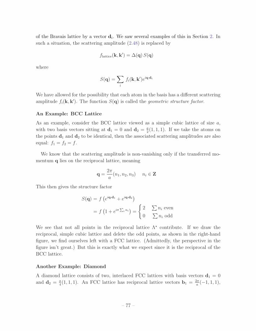
of the Bravais lattice by a vector di. We saw several examples of this in Section 2. In

such a situation, the scattering amplitude (2.48) is replaced by

flattice(k,k′) = ∆(q)S(q)

where

S(q) =∑i

fi(k,k′)eiq·di

We have allowed for the possibility that each atom in the basis has a different scattering

amplitude fi(k,k′). The function S(q) is called the geometric structure factor.

An Example: BCC Lattice

As an example, consider the BCC lattice viewed as a simple cubic lattice of size a,

with two basis vectors sitting at d1 = 0 and d2 = a2(1, 1, 1). If we take the atoms on

the points d1 and d2 to be identical, then the associated scattering amplitudes are also

equal: f1 = f2 = f .

We know that the scattering amplitude is non-vanishing only if the transferred mo-

mentum q lies on the reciprocal lattice, meaning

q =2π

a(n1, n2, n3) ni ∈ Z

This then gives the structure factor

S(q) = f(eiq·d1 + eiq·d2

)= f

(1 + eiπ

∑i ni)

=

2

∑ni even

0∑ni odd

We see that not all points in the reciprocal lattice Λ? contribute. If we draw the

reciprocal, simple cubic lattice and delete the odd points, as shown in the right-hand

figure, we find ourselves left with a FCC lattice. (Admittedly, the perspective in the

figure isn’t great.) But this is exactly what we expect since it is the reciprocal of the

BCC lattice.

Another Example: Diamond

A diamond lattice consists of two, interlaced FCC lattices with basis vectors d1 = 0

and d2 = a4(1, 1, 1). An FCC lattice has reciprocal lattice vectors b1 = 2π

a(−1, 1, 1),

– 77 –

Figure 40: A BCC lattice as cubic lattice

+ basis.

Figure 41: The reciprocal as a cubic lat-

tice minus a basis.

b2 = 2πa

(1,−1, 1) and b3 = 2πa

(1, 1,−1). For q =∑

i nibi, the structure factor is

S(q) = f(1 + ei(π/2)

∑i ni)

=

2

∑ni = 0 mod 4

1 + i∑ni = 1 mod 4

0∑ni = 2 mod 4

1− i∑ni = 3 mod 4

2.4.3 The Debye-Waller Factor

So far, we’ve treated the lattice as a fixed, unmoving object. But we know from our

discussion in Section 4 that this is not realistic. The underlying atoms can move. We

would like to know what effect this has on the scattering off a lattice.

Let’s return to our result (2.48) for the scattering amplitude off a Bravais lattice Λ,

fΛ(k,k′) = f(k,k′)∑n

eiq·Rn

where f(k,k′) is the amplitude for scattering from each site, q = k− k′, and Rn ∈ Λ.

Since the atoms can move, the position Rn are no longer fixed. We should replace

Rn → Rn + un(t)

where, as in Section 4, un describes the deviation of the lattice from equilibrium. In

general, this deviation could arise from either thermal effects or quantum effects. In

keeping with the theme of these lectures, we will restrict to the latter. But this is

conceptually interesting: it means that the scattering amplitude includes the factor

∆(q) =∑n

eiq·Rn eiq·un

which is now a quantum operator. This is telling us something important. When a

particle – whether photon or neutron – scatters off the lattice, it can now excite a

phonon mode. The scattering amplitude is a quantum operator because it includes all

possible end-states of the lattice.

– 78 –

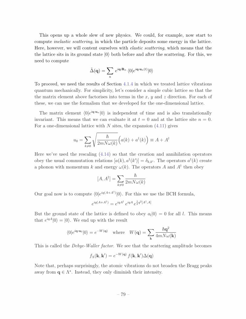
This opens up a whole slew of new physics. We could, for example, now start to

compute inelastic scattering, in which the particle deposits some energy in the lattice.

Here, however, we will content ourselves with elastic scattering, which means that the

the lattice sits in its ground state |0〉 both before and after the scattering. For this, we

need to compute

∆(q) =∑n

eiq·Rn 〈0|eiq·un(t)|0〉

To proceed, we need the results of Section 4.1.4 in which we treated lattice vibrations

quantum mechanically. For simplicity, let’s consider a simple cubic lattice so that the

the matrix element above factorises into terms in the x, y and z direction. For each of

these, we can use the formalism that we developed for the one-dimensional lattice.

The matrix element 〈0|eiq·un|0〉 is independent of time and is also translationally

invariant. This means that we can evaluate it at t = 0 and at the lattice site n = 0.

For a one-dimensional lattice with N sites, the expansion (4.11) gives

u0 =∑k 6=0

√~

2mNω(k)

(a(k) + a†(k)

)≡ A+ A†

Here we’ve used the rescaling (4.14) so that the creation and annihilation operators

obey the usual commutation relations [a(k), a†(k′)] = δk,k′ . The operators a†(k) create

a phonon with momentum k and energy ω(k). The operators A and A† then obey

[A,A†] =∑k 6=0

~2mNω(k)

Our goal now is to compute 〈0|eiq(A+A†)|0〉. For this we use the BCH formula,

eiq(A+A†) = eiqA†eiqA e

12q2[A†,A]

But the ground state of the lattice is defined to obey al|0〉 = 0 for all l. This means

that eiqA|0〉 = |0〉. We end up with the result

〈0|eiq·u0 |0〉 = e−W (q) where W (q) =∑

k

~q2

4mNω(k)

This is called the Debye-Waller factor. We see that the scattering amplitude becomes

fΛ(k,k′) = e−W (q) f(k,k′)∆(q)

Note that, perhaps surprisingly, the atomic vibrations do not broaden the Bragg peaks

away from q ∈ Λ?. Instead, they only diminish their intensity.

– 79 –

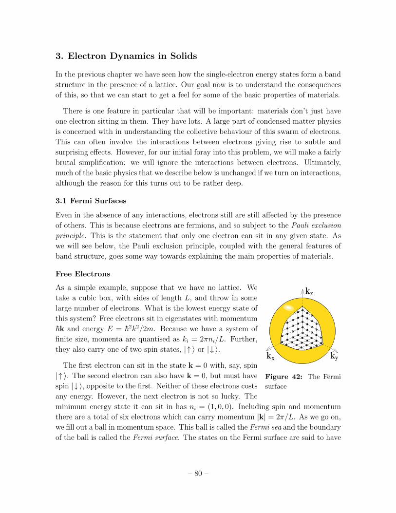
3. Electron Dynamics in Solids

In the previous chapter we have seen how the single-electron energy states form a band

structure in the presence of a lattice. Our goal now is to understand the consequences

of this, so that we can start to get a feel for some of the basic properties of materials.

There is one feature in particular that will be important: materials don’t just have

one electron sitting in them. They have lots. A large part of condensed matter physics

is concerned with in understanding the collective behaviour of this swarm of electrons.

This can often involve the interactions between electrons giving rise to subtle and

surprising effects. However, for our initial foray into this problem, we will make a fairly

brutal simplification: we will ignore the interactions between electrons. Ultimately,

much of the basic physics that we describe below is unchanged if we turn on interactions,

although the reason for this turns out to be rather deep.

3.1 Fermi Surfaces

Even in the absence of any interactions, electrons still are still affected by the presence

of others. This is because electrons are fermions, and so subject to the Pauli exclusion

principle. This is the statement that only one electron can sit in any given state. As

we will see below, the Pauli exclusion principle, coupled with the general features of

band structure, goes some way towards explaining the main properties of materials.

Free Electrons

As a simple example, suppose that we have no lattice. We kz

kk yx

Figure 42: The Fermi

surface

take a cubic box, with sides of length L, and throw in some

large number of electrons. What is the lowest energy state of

this system? Free electrons sit in eigenstates with momentum

~k and energy E = ~2k2/2m. Because we have a system of

finite size, momenta are quantised as ki = 2πni/L. Further,

they also carry one of two spin states, |↑ 〉 or |↓ 〉.

The first electron can sit in the state k = 0 with, say, spin

|↑ 〉. The second electron can also have k = 0, but must have

spin |↓ 〉, opposite to the first. Neither of these electrons costs

any energy. However, the next electron is not so lucky. The

minimum energy state it can sit in has ni = (1, 0, 0). Including spin and momentum

there are a total of six electrons which can carry momentum |k| = 2π/L. As we go on,

we fill out a ball in momentum space. This ball is called the Fermi sea and the boundary

of the ball is called the Fermi surface. The states on the Fermi surface are said to have

– 80 –

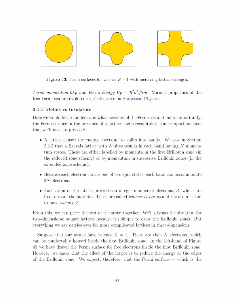
Figure 43: Fermi surfaces for valence Z = 1 with increasing lattice strength.

Fermi momentum ~kF and Fermi energy EF = ~2k2F/2m. Various properties of the

free Fermi sea are explored in the lectures on Statistical Physics.

3.1.1 Metals vs Insulators

Here we would like to understand what becomes of the Fermi sea and, more importantly,

the Fermi surface in the presence of a lattice. Let’s recapitulate some important facts

that we’ll need to proceed:

• A lattice causes the energy spectrum to splits into bands. We saw in Section

2.3.2 that a Bravais lattice with N sites results in each band having N momen-

tum states. These are either labelled by momenta in the first Brillouin zone (in

the reduced zone scheme) or by momentum in successive Brillouin zones (in the

extended zone scheme).

• Because each electron carries one of two spin states, each band can accommodate

2N electrons.

• Each atom of the lattice provides an integer number of electrons, Z, which are

free to roam the material. These are called valence electrons and the atom is said

to have valence Z.

From this, we can piece the rest of the story together. We’ll discuss the situation for

two-dimensional square lattices because it’s simple to draw the Brillouin zones. But

everything we say carries over for more complicated lattices in three-dimensions.

Suppose that our atoms have valence Z = 1. There are then N electrons, which

can be comfortably housed inside the first Brillouin zone. In the left-hand of Figure

43 we have drawn the Fermi surface for free electrons inside the first Brillouin zone.

However, we know that the effect of the lattice is to reduce the energy at the edges

of the Brillouin zone. We expect, therefore, that the Fermi surface — which is the

– 81 –

Figure 44: Lithium. Figure 45: Copper.

equipotential EF — will be distorted as shown in the middle figure, with states closer

to the edge of the Brillouin zone filled preferentially. Note that the area inside the

Fermi surface remains the same.

If the effects of the lattice get very strong, it may be that the Fermi surface touches

the edge of the Brillouin zone as shown in the right-hand drawing in Figure 43. Because

the Brillouin zone is a torus, if the Fermi surface is to be smooth then it must hit the

edge of the Brillouin zone at right-angles.

This same physics can be seen in real Fermi surfaces. Lithium has valence Z = 1.

It forms a BCC lattice, and so the Brillouin zone is FCC. Its Fermi surface is shown

above, plotted within its Brillouin zone2. Copper also has valency Z = 1, with a FCC

lattice and hence BCC Brillouin zone. Here the effects of the lattice are somewhat

stronger, and the Fermi surface touches the Brillouin zone.

In all of these cases, there are unoccupied states with arbitrarily small energy above

EF . (Strictly speaking, this statement holds only in the limit L → ∞ of an infinitely

large lattice.) This means that if we perturb the system in any way, the electrons will

easily be able to respond. Note, however, that only those electrons close to the Fermi

surface can respond; those that lie deep within the Fermi sea are locked there by the

Pauli exclusion principle and require much larger amounts of energy if they wish to

escape.

This is an important point, so I’ll say it again. In most situations, only those electrons

which lie on the Fermi surface can actually do anything. This is why Fermi surfaces

play such a crucial role in our understanding of materials.

2This, and other pictures of Fermi surfaces, are taken from http://www.phys.ufl.edu/fermisurface/.

– 82 –

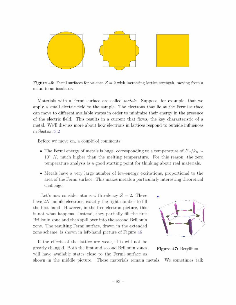
Figure 46: Fermi surfaces for valence Z = 2 with increasing lattice strength, moving from a

metal to an insulator.

Materials with a Fermi surface are called metals. Suppose, for example, that we

apply a small electric field to the sample. The electrons that lie at the Fermi surface

can move to different available states in order to minimize their energy in the presence

of the electric field. This results in a current that flows, the key characteristic of a

metal. We’ll discuss more about how electrons in lattices respond to outside influences

in Section 3.2

Before we move on, a couple of comments:

• The Fermi energy of metals is huge, corresponding to a temperature of EF/kB ∼104 K, much higher than the melting temperature. For this reason, the zero

temperature analysis is a good starting point for thinking about real materials.

• Metals have a very large number of low-energy excitations, proportional to the

area of the Fermi surface. This makes metals a particularly interesting theoretical

challenge.

Let’s now consider atoms with valency Z = 2. These

Figure 47: Beryllium

have 2N mobile electrons, exactly the right number to fill

the first band. However, in the free electron picture, this

is not what happens. Instead, they partially fill the first

Brillouin zone and then spill over into the second Brillouin

zone. The resulting Fermi surface, drawn in the extended

zone scheme, is shown in left-hand picture of Figure 46

If the effects of the lattice are weak, this will not be

greatly changed. Both the first and second Brillouin zones

will have available states close to the Fermi surface as

shown in the middle picture. These materials remain metals. We sometimes talk

– 83 –

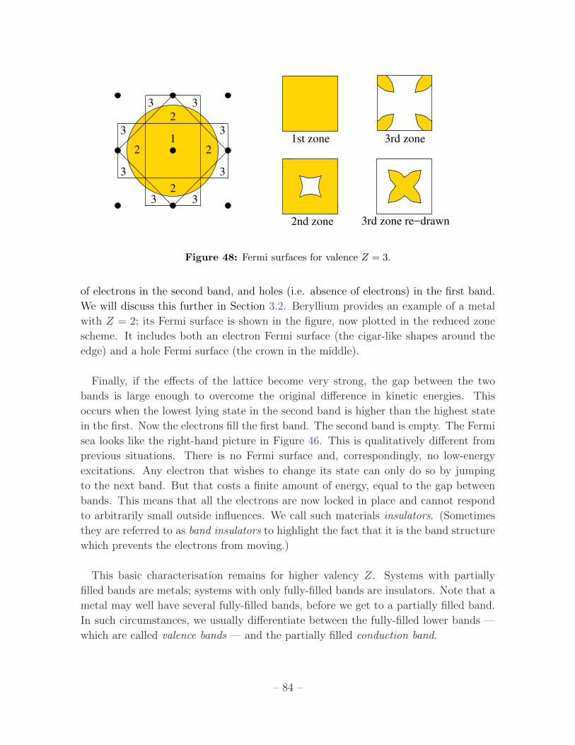
1

2 2

2

2

3 3

3

3

33

3

31st zone

2nd zone

3rd zone

3rd zone re−drawn

Figure 48: Fermi surfaces for valence Z = 3.

of electrons in the second band, and holes (i.e. absence of electrons) in the first band.

We will discuss this further in Section 3.2. Beryllium provides an example of a metal

with Z = 2; its Fermi surface is shown in the figure, now plotted in the reduced zone

scheme. It includes both an electron Fermi surface (the cigar-like shapes around the

edge) and a hole Fermi surface (the crown in the middle).

Finally, if the effects of the lattice become very strong, the gap between the two

bands is large enough to overcome the original difference in kinetic energies. This

occurs when the lowest lying state in the second band is higher than the highest state

in the first. Now the electrons fill the first band. The second band is empty. The Fermi

sea looks like the right-hand picture in Figure 46. This is qualitatively different from

previous situations. There is no Fermi surface and, correspondingly, no low-energy

excitations. Any electron that wishes to change its state can only do so by jumping

to the next band. But that costs a finite amount of energy, equal to the gap between

bands. This means that all the electrons are now locked in place and cannot respond

to arbitrarily small outside influences. We call such materials insulators. (Sometimes

they are referred to as band insulators to highlight the fact that it is the band structure

which prevents the electrons from moving.)

This basic characterisation remains for higher valency Z. Systems with partially

filled bands are metals; systems with only fully-filled bands are insulators. Note that a

metal may well have several fully-filled bands, before we get to a partially filled band.

In such circumstances, we usually differentiate between the fully-filled lower bands —

which are called valence bands — and the partially filled conduction band.

– 84 –

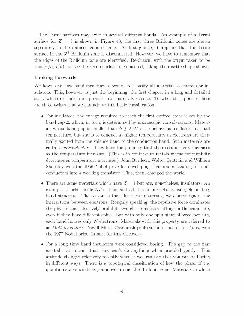
The Fermi surfaces may exist in several different bands. An example of a Fermi

surface for Z = 3 is shown in Figure 48, the first three Brillouin zones are shown

separately in the reduced zone scheme. At first glance, it appears that the Fermi

surface in the 3rd Brillouin zone is disconnected. However, we have to remember that

the edges of the Brillouin zone are identified. Re-drawn, with the origin taken to be

k = (π/a, π/a), we see the Fermi surface is connected, taking the rosette shape shown.

Looking Forwards

We have seen how band structure allows us to classify all materials as metals or in-

sulators. This, however, is just the beginning, the first chapter in a long and detailed

story which extends from physics into materials science. To whet the appetite, here

are three twists that we can add to this basic classification.

• For insulators, the energy required to reach the first excited state is set by the

band gap ∆ which, in turn, is determined by microscopic considerations. Materi-

als whose band gap is smaller than ∆ . 2 eV or so behave as insulators at small

temperature, but starts to conduct at higher temperatures as electrons are ther-

mally excited from the valence band to the conduction band. Such materials are

called semiconductors. They have the property that their conductivity increases

as the temperature increases. (This is in contrast to metals whose conductivity

decreases as temperature increases.) John Bardeen, Walter Brattain and William

Shockley won the 1956 Nobel prize for developing their understanding of semi-

conductors into a working transistor. This, then, changed the world.

• There are some materials which have Z = 1 but are, nonetheless, insulators. An

example is nickel oxide NiO. This contradicts our predictions using elementary

band structure. The reason is that, for these materials, we cannot ignore the

interactions between electrons. Roughly speaking, the repulsive force dominates

the physics and effectively prohibits two electrons from sitting on the same site,

even if they have different spins. But with only one spin state allowed per site,

each band houses only N electrons. Materials with this property are referred to

as Mott insulators. Nevill Mott, Cavendish professor and master of Caius, won

the 1977 Nobel prize, in part for this discovery.

• For a long time band insulators were considered boring. The gap to the first

excited state means that they can’t do anything when prodded gently. This

attitude changed relatively recently when it was realised that you can be boring

in different ways. There is a topological classification of how the phase of the

quantum states winds as you move around the Brillouin zone. Materials in which

– 85 –

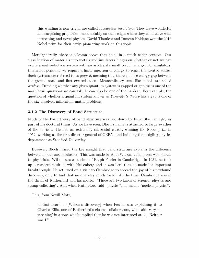
this winding is non-trivial are called topological insulators. They have wonderful

and surprising properties, most notably on their edges where they come alive with

interesting and novel physics. David Thouless and Duncan Haldane won the 2016

Nobel prize for their early, pioneering work on this topic.

More generally, there is a lesson above that holds in a much wider context. Our

classification of materials into metals and insulators hinges on whether or not we can

excite a multi-electron system with an arbitrarily small cost in energy. For insulators,

this is not possible: we require a finite injection of energy to reach the excited states.

Such systems are referred to as gapped, meaning that there is finite energy gap between

the ground state and first excited state. Meanwhile, systems like metals are called

gapless. Deciding whether any given quantum system is gapped or gapless is one of the

most basic questions we can ask. It can also be one of the hardest. For example, the

question of whether a quantum system known as Yang-Mills theory has a gap is one of

the six unsolved milllenium maths problems.

3.1.2 The Discovery of Band Structure

Much of the basic theory of band structure was laid down by Felix Bloch in 1928 as

part of his doctoral thesis. As we have seen, Bloch’s name is attached to large swathes

of the subject. He had an extremely successful career, winning the Nobel prize in

1952, working as the first director-general of CERN, and building the fledgling physics

department at Stanford University.

However, Bloch missed the key insight that band structure explains the difference

between metals and insulators. This was made by Alan Wilson, a name less well known

to physicists. Wilson was a student of Ralph Fowler in Cambridge. In 1931, he took

up a research position with Heisenberg and it was here that he made his important

breakthrough. He returned on a visit to Cambridge to spread the joy of his newfound

discovery, only to find that no one very much cared. At the time, Cambridge was in

the thrall of Rutherford and his motto: “There are two kinds of science, physics and

stamp collecting”. And when Rutherford said “physics”, he meant “nuclear physics”.

This, from Nevill Mott,

“I first heard of [Wilson’s discovery] when Fowler was explaining it to

Charles Ellis, one of Rutherford’s closest collaborators, who said ‘very in-

teresting’ in a tone which implied that he was not interested at all. Neither

was I.”

– 86 –

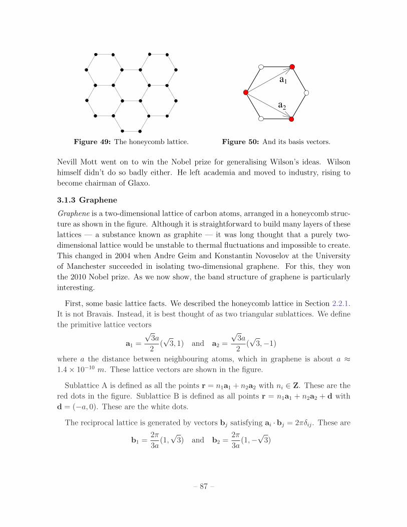
a2

a1

Figure 49: The honeycomb lattice. Figure 50: And its basis vectors.

Nevill Mott went on to win the Nobel prize for generalising Wilson’s ideas. Wilson

himself didn’t do so badly either. He left academia and moved to industry, rising to

become chairman of Glaxo.

3.1.3 Graphene

Graphene is a two-dimensional lattice of carbon atoms, arranged in a honeycomb struc-

ture as shown in the figure. Although it is straightforward to build many layers of these

lattices — a substance known as graphite — it was long thought that a purely two-

dimensional lattice would be unstable to thermal fluctuations and impossible to create.

This changed in 2004 when Andre Geim and Konstantin Novoselov at the University

of Manchester succeeded in isolating two-dimensional graphene. For this, they won

the 2010 Nobel prize. As we now show, the band structure of graphene is particularly

interesting.

First, some basic lattice facts. We described the honeycomb lattice in Section 2.2.1.

It is not Bravais. Instead, it is best thought of as two triangular sublattices. We define

the primitive lattice vectors

a1 =

√3a

2(√

3, 1) and a2 =

√3a

2(√

3,−1)

where a the distance between neighbouring atoms, which in graphene is about a ≈1.4× 10−10 m. These lattice vectors are shown in the figure.

Sublattice A is defined as all the points r = n1a1 + n2a2 with ni ∈ Z. These are the

red dots in the figure. Sublattice B is defined as all points r = n1a1 + n2a2 + d with

d = (−a, 0). These are the white dots.

The reciprocal lattice is generated by vectors bj satisfying ai ·bj = 2πδij. These are

b1 =2π

3a(1,√

3) and b2 =2π

3a(1,−

√3)

– 87 –

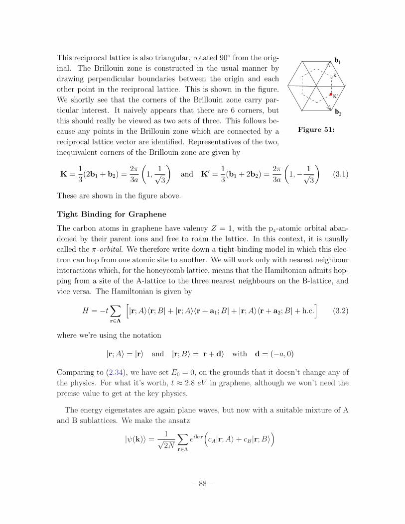
This reciprocal lattice is also triangular, rotated 90 from the orig-

b2

b1

K

K’

Figure 51:

inal. The Brillouin zone is constructed in the usual manner by

drawing perpendicular boundaries between the origin and each

other point in the reciprocal lattice. This is shown in the figure.

We shortly see that the corners of the Brillouin zone carry par-

ticular interest. It naively appears that there are 6 corners, but

this should really be viewed as two sets of three. This follows be-

cause any points in the Brillouin zone which are connected by a

reciprocal lattice vector are identified. Representatives of the two,

inequivalent corners of the Brillouin zone are given by

K =1

3(2b1 + b2) =

2π

3a

(1,

1√3

)and K′ =

1

3(b1 + 2b2) =

2π

3a

(1,− 1√

3

)(3.1)

These are shown in the figure above.

Tight Binding for Graphene

The carbon atoms in graphene have valency Z = 1, with the pz-atomic orbital aban-

doned by their parent ions and free to roam the lattice. In this context, it is usually

called the π-orbital. We therefore write down a tight-binding model in which this elec-

tron can hop from one atomic site to another. We will work only with nearest neighbour

interactions which, for the honeycomb lattice, means that the Hamiltonian admits hop-

ping from a site of the A-lattice to the three nearest neighbours on the B-lattice, and

vice versa. The Hamiltonian is given by

H = −t∑r∈Λ

[|r;A〉〈r;B|+ |r;A〉〈r + a1;B|+ |r;A〉〈r + a2;B|+ h.c.

](3.2)

where we’re using the notation

|r;A〉 = |r〉 and |r;B〉 = |r + d〉 with d = (−a, 0)

Comparing to (2.34), we have set E0 = 0, on the grounds that it doesn’t change any of

the physics. For what it’s worth, t ≈ 2.8 eV in graphene, although we won’t need the

precise value to get at the key physics.

The energy eigenstates are again plane waves, but now with a suitable mixture of A

and B sublattices. We make the ansatz

|ψ(k)〉 =1√2N

∑r∈Λ

eik·r(cA|r;A〉+ cB|r;B〉

)

– 88 –

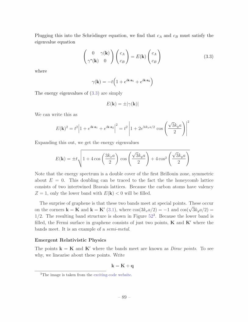
Plugging this into the Schrodinger equation, we find that cA and cB must satisfy the

eigenvalue equation (0 γ(k)

γ?(k) 0

)(cA

cB

)= E(k)

(cA

cB

)(3.3)

where

γ(k) = −t(

1 + eik·a1 + eik·a2

)The energy eigenvalues of (3.3) are simply

E(k) = ±|γ(k)|

We can write this as

E(k)2 = t2∣∣∣1 + eik·a1 + eik·a2

∣∣∣2 = t2

∣∣∣∣∣1 + 2e3ikxa/2 cos

(√3kya

2

)∣∣∣∣∣2

Expanding this out, we get the energy eigenvalues

E(k) = ±t

√√√√1 + 4 cos

(3kxa

2

)cos

(√3kya

2

)+ 4 cos2

(√3kya

2

)

Note that the energy spectrum is a double cover of the first Brillouin zone, symmetric

about E = 0. This doubling can be traced to the fact the the honeycomb lattice

consists of two intertwined Bravais lattices. Because the carbon atoms have valency

Z = 1, only the lower band with E(k) < 0 will be filled.

The surprise of graphene is that these two bands meet at special points. These occur

on the corners k = K and k = K′ (3.1), where cos(3kxa/2) = −1 and cos(√

3kya/2) =

1/2. The resulting band structure is shown in Figure 523. Because the lower band is

filled, the Fermi surface in graphene consists of just two points, K and K′ where the

bands meet. It is an example of a semi-metal.

Emergent Relativistic Physics

The points k = K and K′ where the bands meet are known as Dirac points. To see

why, we linearise about these points. Write

k = K + q

3The image is taken from the exciting-code website.

– 89 –

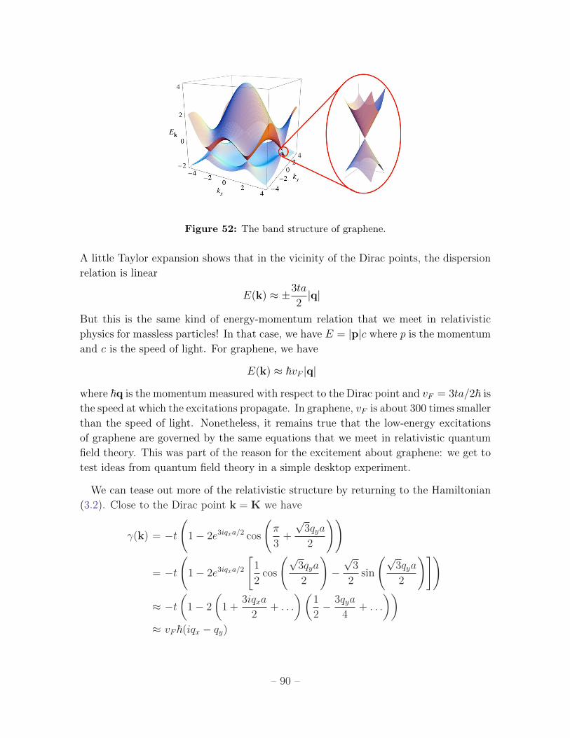
Figure 52: The band structure of graphene.

A little Taylor expansion shows that in the vicinity of the Dirac points, the dispersion

relation is linear

E(k) ≈ ±3ta

2|q|

But this is the same kind of energy-momentum relation that we meet in relativistic

physics for massless particles! In that case, we have E = |p|c where p is the momentum

and c is the speed of light. For graphene, we have

E(k) ≈ ~vF |q|

where ~q is the momentum measured with respect to the Dirac point and vF = 3ta/2~ is

the speed at which the excitations propagate. In graphene, vF is about 300 times smaller

than the speed of light. Nonetheless, it remains true that the low-energy excitations

of graphene are governed by the same equations that we meet in relativistic quantum

field theory. This was part of the reason for the excitement about graphene: we get to

test ideas from quantum field theory in a simple desktop experiment.

We can tease out more of the relativistic structure by returning to the Hamiltonian

(3.2). Close to the Dirac point k = K we have

γ(k) = −t

(1− 2e3iqxa/2 cos

(π

3+

√3qya

2

))

= −t

(1− 2e3iqxa/2

[1

2cos

(√3qya

2

)−√

3

2sin

(√3qya

2

)])

≈ −t(

1− 2

(1 +

3iqxa

2+ . . .

)(1

2− 3qya

4+ . . .

))≈ vF~(iqx − qy)

– 90 –

This means that the Hamiltonian in the vicinity of the Dirac point k = K takes the

form

H = vF~

(0 iqx − qy

−iqx − qy 0

)= −vF~(qxσ

y + qyσx) (3.4)

where σx and σy are the Pauli matrices. But this is the Dirac equation for a massless

particle moving in two-dimensions, sometimes referred to as the Pauli equation. (Note:

our original choice of orientation of the honeycomb lattice has resulted in a slightly

annoying expression for the Hamiltonian. Had we rotated by 90 to begin with, we

would be left with the nicer H = ~vF q · σ where σ = (σx, σy).)

There’s something of an irony here. In the original Dirac equation, the 2× 2 matrix

structure comes about because the electron carries spin. But that’s not the origin of the

matrix structure in (3.4). Indeed, we’ve not mentioned spin anywhere in our discussion.

Instead, in graphene the emergent “spin” degree of freedom arises from the existence

of the two A and B sublattices.

We get a very similar equation in the vicinity of the other Dirac point. Expanding

k = K′ + q′, we get the resulting Hamiltonian

H = −vF~(qxσy − qyσx)

The difference in minus sign is sometimes said to be a different handedness or helicity.

You will learn more about this in the context of high energy physics in the lectures on

Quantum Field Theory.

As we mentioned above, we have not yet included the spin of the electron. This is

trivial: the discussion above is simply repeated twice, once for spin | ↑ 〉 and once for

spin | ↓ 〉. The upshot is that the low-energy excitations of graphene are described by

four massless Dirac fermions. One pair comes from the spin degeneracy of the electrons;

the other from the existence of two Dirac points K and K′, sometimes referred to as

the valley degeneracy.

3.2 Dynamics of Bloch Electrons

In this section, we look more closely at how electrons moving in a lattice environment

react to external forces. We call these electrons Bloch electrons. We start by describing

how some familiar quantities are redefined for Bloch electrons.

– 91 –

For simplicity, consider an insulator and throw in one further electron. This solitary

electron sits all alone in an otherwise unoccupied band. The possible states available

to it have energy E(k) where k lies in the first Brillouin zone. (The energy should also

have a further discrete index which labels the particular band the electron is sitting in,

but we’ll suppress this in what follows). Despite its environment, we can still assign

some standard properties to this electron.

3.2.1 Velocity

The average velocity v of the electron is

v =1

~∂E

∂k(3.5)

First note that this is simply the group velocity of a wavepacket (a concept that we’ve

met previously in the lectures on Electromagnetism). However, the “average velocity”

means something specific in quantum mechanics, and to prove (3.5) we should directly

compute v = 1m〈ψ| − i~∇|ψ〉.

Bloch’s theorem ensures that the electron eigenstates take the form

ψk(x) = eik·x uk(x)

with k in the Brillouin zone. As with the energy, we’ve suppressed the discrete band

index on the wavefunction. The full wavefunction satisfies Hψk(x) = E(k)ψk(x), so

that uk(x) obeys

Hkuk(x) = E(k)uk(x) with Hk =~2

2m(−i∇+ k)2 + V (x) (3.6)

We’ll use a slick trick. Consider the Hamiltonian Hk+q which we expand as

Hk+q = Hk +∂Hk

∂k· q +

1

2

∂2Hk

∂ki∂kjqiqj (3.7)

For small q, we view this as a perturbation of Hk. From our results of first order

perturbation theory, we know that the shift of the energy eigenvalues is

∆E = 〈uk|∂Hk

∂k· q|uk〉

But we also know the exact result: it is simply E(k + q). Expanding this to first order

in q, we have the result

〈uk|∂Hk

∂k|uk〉 =

∂E

∂k

– 92 –

But this is exactly what we need. Using the expression (3.6) for Hk, the left-hand side

is

~2

m〈uk|(−i∇+ k)|uk〉 =

~m〈ψk| − i~∇|ψk〉 = ~v

This gives our desired result (3.5).

It is perhaps surprising that eigenstates in a crystal have a fixed, average velocity.

One might naively expect that the particle would collide with the crystal, bouncing

all over the place with a corresponding vanishing average velocity. Yet the beauty of

Bloch’s theorem is that this is not what happens. The electrons can quite happily glide

through the crystal structure.

A Filled Band Carries Neither Current nor Heat

Before we go on, we can use the above result to prove a simple result: a completely

filled band does not contribute to the current. This is true whether the filled band is

part of an insulator, or part of a metal. (In the latter case, there will also be a partially

filled band which will contribute to the current.)

The current carried by each electron is j = −ev where −e is the electron charge.

From (3.5), the total current of a filled band is then

j = −2e

~

∫BZ

d3k

(2π)3

∂E

∂k(3.8)

where the overall factor of 2 counts the spin degeneracy. This integral vanishes. This

follows because E(k) is a periodic function over the Brillouin zone and the total deriva-

tive of any periodic function always integrates to zero.

Alternatively, if the crystal has an inversion symmetry then there is a more di-

rect proof. The energy satisfies E(k) = E(−k), which means that ∂E(k)/∂k =

−∂E(−k)/∂k and the contributions to the integral cancel between the two halves of

the Brillouin zone.

The same argument shows that a filled band cannot transport energy in the form of

heat. The heat current is defined as

jE = 2

∫BZ

d3k

(2π)3Ev =

1

~

∫BZ

d3k

(2π)3

∂(E2)

∂k

which again vanishes when integrated over a filled band. This means that the electrons

trapped in insulators can conduct neither electricity nor heat. Note, however, that

while there is nothing else charged that can conduct electricity, there are other degrees

of freedom – in particular, phonons – which can conduct heat.

– 93 –

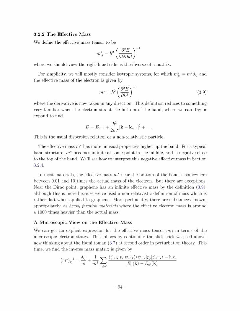
3.2.2 The Effective Mass

We define the effective mass tensor to be

m?ij = ~2

(∂2E

∂ki∂kj

)−1

where we should view the right-hand side as the inverse of a matrix.

For simplicity, we will mostly consider isotropic systems, for which m?ij = m?δij and

the effective mass of the electron is given by

m? = ~2

(∂2E

∂k2

)−1

(3.9)

where the derivative is now taken in any direction. This definition reduces to something

very familiar when the electron sits at the bottom of the band, where we can Taylor

expand to find

E = Emin +~2

2m?|k− kmin|2 + . . .

This is the usual dispersion relation or a non-relativistic particle.

The effective mass m? has more unusual properties higher up the band. For a typical

band structure, m? becomes infinite at some point in the middle, and is negative close

to the top of the band. We’ll see how to interpret this negative effective mass in Section

3.2.4.

In most materials, the effective mass m? near the bottom of the band is somewhere

between 0.01 and 10 times the actual mass of the electron. But there are exceptions.

Near the Dirac point, graphene has an infinite effective mass by the definition (3.9),

although this is more because we’ve used a non-relativistic definition of mass which is

rather daft when applied to graphene. More pertinently, there are substances known,

appropriately, as heavy fermion materials where the effective electron mass is around

a 1000 times heavier than the actual mass.

A Microscopic View on the Effective Mass

We can get an explicit expression for the effective mass tensor mij in terms of the

microscopic electron states. This follows by continuing the slick trick we used above,

now thinking about the Hamiltonian (3.7) at second order in perturbation theory. This

time, we find the inverse mass matrix is given by

(m?)−1ij =

δijm

+1

m2

∑n 6=n′

〈ψn,k|pi|ψn′,k〉〈ψn,k|pj|ψn′,k〉 − h.c.

En(k)− En′(k)

– 94 –

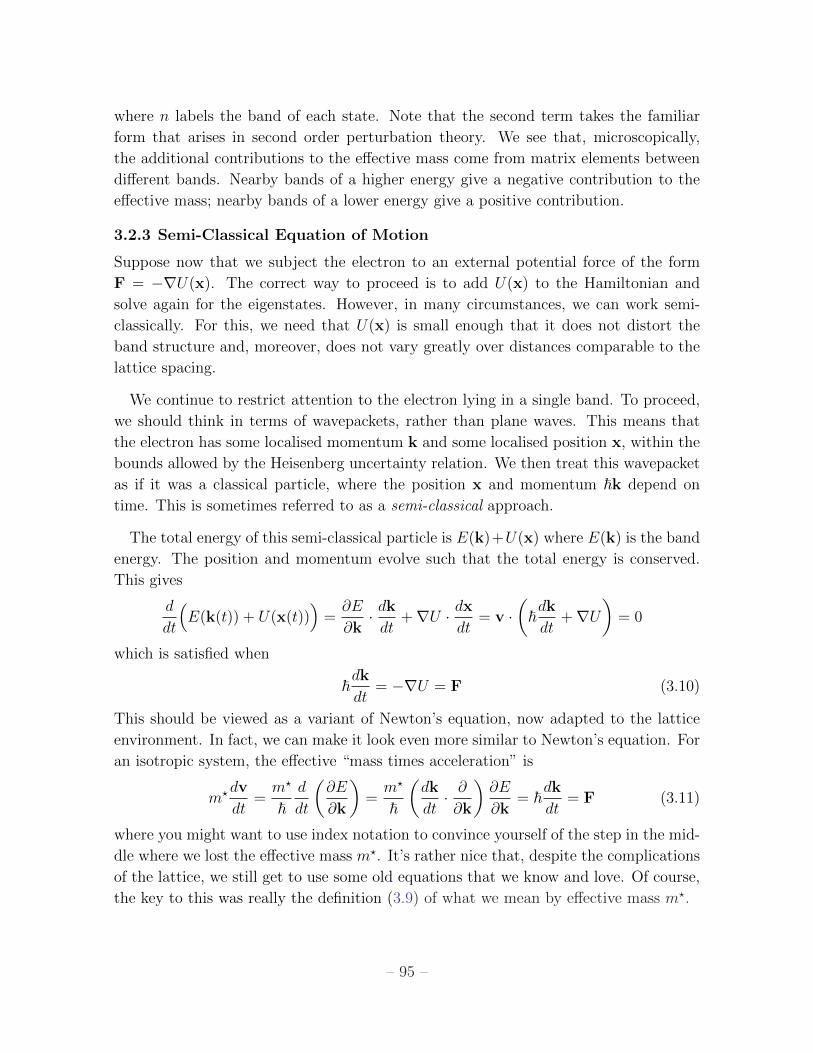
where n labels the band of each state. Note that the second term takes the familiar

form that arises in second order perturbation theory. We see that, microscopically,

the additional contributions to the effective mass come from matrix elements between

different bands. Nearby bands of a higher energy give a negative contribution to the

effective mass; nearby bands of a lower energy give a positive contribution.

3.2.3 Semi-Classical Equation of Motion

Suppose now that we subject the electron to an external potential force of the form

F = −∇U(x). The correct way to proceed is to add U(x) to the Hamiltonian and

solve again for the eigenstates. However, in many circumstances, we can work semi-

classically. For this, we need that U(x) is small enough that it does not distort the

band structure and, moreover, does not vary greatly over distances comparable to the

lattice spacing.

We continue to restrict attention to the electron lying in a single band. To proceed,

we should think in terms of wavepackets, rather than plane waves. This means that

the electron has some localised momentum k and some localised position x, within the

bounds allowed by the Heisenberg uncertainty relation. We then treat this wavepacket

as if it was a classical particle, where the position x and momentum ~k depend on

time. This is sometimes referred to as a semi-classical approach.

The total energy of this semi-classical particle is E(k)+U(x) where E(k) is the band

energy. The position and momentum evolve such that the total energy is conserved.

This gives

d

dt

(E(k(t)) + U(x(t))

)=∂E

∂k· dkdt

+∇U · dxdt

= v ·(~dk

dt+∇U

)= 0

which is satisfied when

~dk

dt= −∇U = F (3.10)

This should be viewed as a variant of Newton’s equation, now adapted to the lattice

environment. In fact, we can make it look even more similar to Newton’s equation. For

an isotropic system, the effective “mass times acceleration” is

m?dv

dt=m?

~d

dt

(∂E

∂k

)=m?

~

(dk

dt· ∂∂k

)∂E

∂k= ~

dk

dt= F (3.11)

where you might want to use index notation to convince yourself of the step in the mid-

dle where we lost the effective mass m?. It’s rather nice that, despite the complications

of the lattice, we still get to use some old equations that we know and love. Of course,

the key to this was really the definition (3.9) of what we mean by effective mass m?.

– 95 –

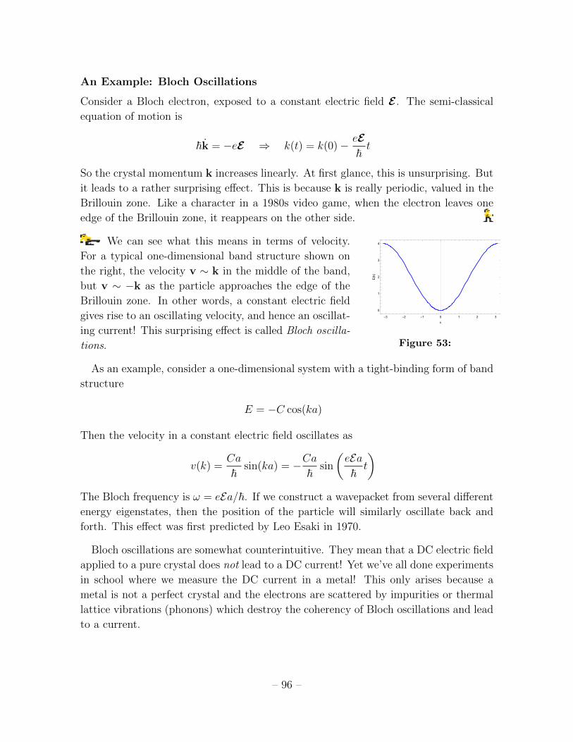
An Example: Bloch Oscillations

Consider a Bloch electron, exposed to a constant electric field E . The semi-classical

equation of motion is

~k = −eE ⇒ k(t) = k(0)− eE~t

So the crystal momentum k increases linearly. At first glance, this is unsurprising. But

it leads to a rather surprising effect. This is because k is really periodic, valued in the

Brillouin zone. Like a character in a 1980s video game, when the electron leaves one

edge of the Brillouin zone, it reappears on the other side.

We can see what this means in terms of velocity.

-3 -2 -1 0 1 2 3

0

1

2

3

4

k

E(k)

Figure 53:

For a typical one-dimensional band structure shown on

the right, the velocity v ∼ k in the middle of the band,

but v ∼ −k as the particle approaches the edge of the

Brillouin zone. In other words, a constant electric field

gives rise to an oscillating velocity, and hence an oscillat-

ing current! This surprising effect is called Bloch oscilla-

tions.

As an example, consider a one-dimensional system with a tight-binding form of band

structure

E = −C cos(ka)

Then the velocity in a constant electric field oscillates as

v(k) =Ca

~sin(ka) = −Ca

~sin

(eEa~t

)The Bloch frequency is ω = eEa/~. If we construct a wavepacket from several different

energy eigenstates, then the position of the particle will similarly oscillate back and

forth. This effect was first predicted by Leo Esaki in 1970.

Bloch oscillations are somewhat counterintuitive. They mean that a DC electric field

applied to a pure crystal does not lead to a DC current! Yet we’ve all done experiments

in school where we measure the DC current in a metal! This only arises because a

metal is not a perfect crystal and the electrons are scattered by impurities or thermal

lattice vibrations (phonons) which destroy the coherency of Bloch oscillations and lead

to a current.

– 96 –

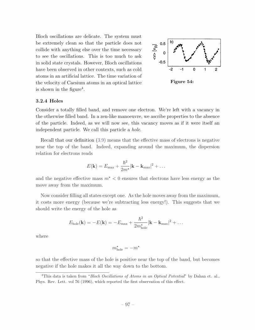
Bloch oscillations are delicate. The system must

Figure 54:

be extremely clean so that the particle does not

collide with anything else over the time necessary

to see the oscillations. This is too much to ask

in solid state crystals. However, Bloch oscillations

have been observed in other contexts, such as cold

atoms in an artificial lattice. The time variation of

the velocity of Caesium atoms in an optical lattice

is shown in the figure4.

3.2.4 Holes

Consider a totally filled band, and remove one electron. We’re left with a vacancy in

the otherwise filled band. In a zen-like manoeuvre, we ascribe properties to the absence

of the particle. Indeed, as we will now see, this vacancy moves as if it were itself an

independent particle. We call this particle a hole.

Recall that our definition (3.9) means that the effective mass of electrons is negative

near the top of the band. Indeed, expanding around the maximum, the dispersion

relation for electrons reads

E(k) = Emax +~2

2m?|k− kmax|2 + . . .

and the negative effective mass m? < 0 ensures that electrons have less energy as the

move away from the maximum.

Now consider filling all states except one. As the hole moves away from the maximum,

it costs more energy (because we’re subtracting less energy!). This suggests that we

should write the energy of the hole as

Ehole(k) = −E(k) = −Emax +~2

2m?hole

|k− kmax|2 + . . .

where

m?hole = −m?

so that the effective mass of the hole is positive near the top of the band, but becomes

negative if the hole makes it all the way down to the bottom.

4This data is taken from “Bloch Oscillations of Atoms in an Optical Potential” by Dahan et. al.,

Phys. Rev. Lett. vol 76 (1996), which reported the first observation of this effect.

– 97 –

The hole has other properties. Suppose that we take away an electron with momen-

tum k. Then the resulting hole can be thought of as having momentum −k. This

suggests that we define

khole = −k (3.12)

However, the velocity of the hole is the same as that of the missing electron

vhole =1

~∂Ehole

∂khole

=1

~∂E

∂k= v

This too is intuitive, since the hole is moving in the same direction as the electron that

we took away.

The definitions above mean that the hole obeys the Newtonian force law with

m?hole

dvhole

dt= −F = Fhole (3.13)

At first sight, this is surprising: the hole experiences an opposite force to the electron.

But there’s a very simple interpretation. The force that we typically wish to apply to

our system is an electric field E which, for an electron, gives rise to

F = −eE

The minus sign in (3.13) is simply telling us that the hole should be thought of as

carrying charge +e, the opposite of the electron,

Fhole = +eE

We can also reach this same conclusion by computing the current. We saw in (3.8)

that a fully filled band carries no current. This means that the current carried by a

partially filled band is

j = −2e

∫filled

d3k

(2π)3v(k) = +2e

∫unfilled

d3k

(2π)3v(k)

The filled states are electrons carrying charge −e; the unfilled states are holes, carrying

charge +e.

Finally, it’s worth mentioning that the idea of holes in band structure provides a fairly

decent analogy for anti-matter in high-energy physics. There too the electron has a

positively charged cousin, now called the positron. In both cases, the two particles can

come together and annihilate. In solids, this releases a few eV of energy, given by the

gap between bands. In high-energy physics, this releases a million times more energy,

given by the rest mass of the electron.

– 98 –

3.2.5 Drude Model Again

The essence of Bloch’s theorem is that electrons can travel through perfect crystals

unimpeded. And yet, in the real world, this does not happen. Even the best metals have

a resistance, in which any current degrades and ultimately relaxes to zero. This happens

because metals are not perfect crystals, and the electrons collide with impurities and

vacancies, as well as thermally vibrations called phonons.

We can model these effects in our semi-classical description by working with the

electron equation of motion called the Drude model

m?v = −eE − m?

τv (3.14)

Here E is the applied electric field and τ is the scattering time, which should be thought

of as the average time between collisions.

We have already met the Drude model in the lectures on Electromagnetism when

we tried to describe the conductivity in metals classically. We have now included the

quantum effects of lattices and the Fermi surface yet, rather remarkably, the equation

remains essentially unchanged. The only difference is that the effective mass m? will

depend on k, and hence on v, if the electron is not close to the minimum of the band.

In equilibrium, the velocity of the electron is

v = − eτm?

E (3.15)

The proportionality constant is called the mobility, µ = |eτ/m?|. The total current

density j = −env where n is the density of charge carriers. The equation (3.15) then

becomes j = σE where σ is the conductivity,

σ =e2τn

m?(3.16)

We also define the resistivity ρ = 1/σ. This is the same result that we found in our

earlier classical analysis, except the mass m is replaced by the effective mass m?.

There is, however, one crucial difference that the existence of the Fermi surface has

introduced. When bands are mostly unfilled, it is best to think of the charge carriers

in terms of negatively charged electrons, with positive effective mass m?. But when

bands are mostly filled, it is best to think of the charge carriers in terms of positively

charged holes, also with positive mass m?hole. In this case, we should replace the Drude

model (3.14) with the equivalent version for holes,

m?holev = +eE − m?

hole

τv (3.17)

– 99 –

This means that certain materials can appear to have positive charge carriers, even

though the only things actually moving are electrons. The different sign in the charge

carrier doesn’t show up in the conductivity (3.16), which depends on e2. To see it, we

need to throw in an extra ingredient.

Hall Resistivity

The standard technique to measure the charge of a material is to apply a magnetic

field B. Classically, particles of opposite charges will bend in a opposite directions,

perpendicular to B. In a material, this results in the classical Hall effect.

We will discuss the motion of Bloch electrons in a magnetic field in much more

detail in Section 3.3. (And we will discuss the Hall effect in much much more detail

in other lectures.) Here, we simply want to show how this effect reveals the difference

between electrons and holes. For electrons, we adapt the Drude model (3.14) by adding

a Lorentz force,

m?v = −e(E + v ×B)− m?

τv

We once again look for equilibrium solutions with v = 0. Writing j = −nev, we now

must solve the vector equation

1

nej×B +

m?

ne2τj = E

The solution to this is

E = ρj

where the resistivity ρ is now a 3× 3 matrix. If we take B = (0, 0, B), then we have

ρ =

ρxx ρxy 0

−ρxy ρxx 0

0 0 ρxx

where the diagonal, longitudinal resistivity is ρxx = 1/σ where σ is given in (3.16). The

novelty is the off-diagonal, Hall resistivity

ρxy =B

neWe often define the Hall coefficient RH as

RH =ρxyB

=1

neThis, as promised, depends on the charge e. This means that if we were to repeat the

above analysis for holes (3.17) rather than electrons, we would find a Hall coefficient

which differs by a minus sign.

– 100 –

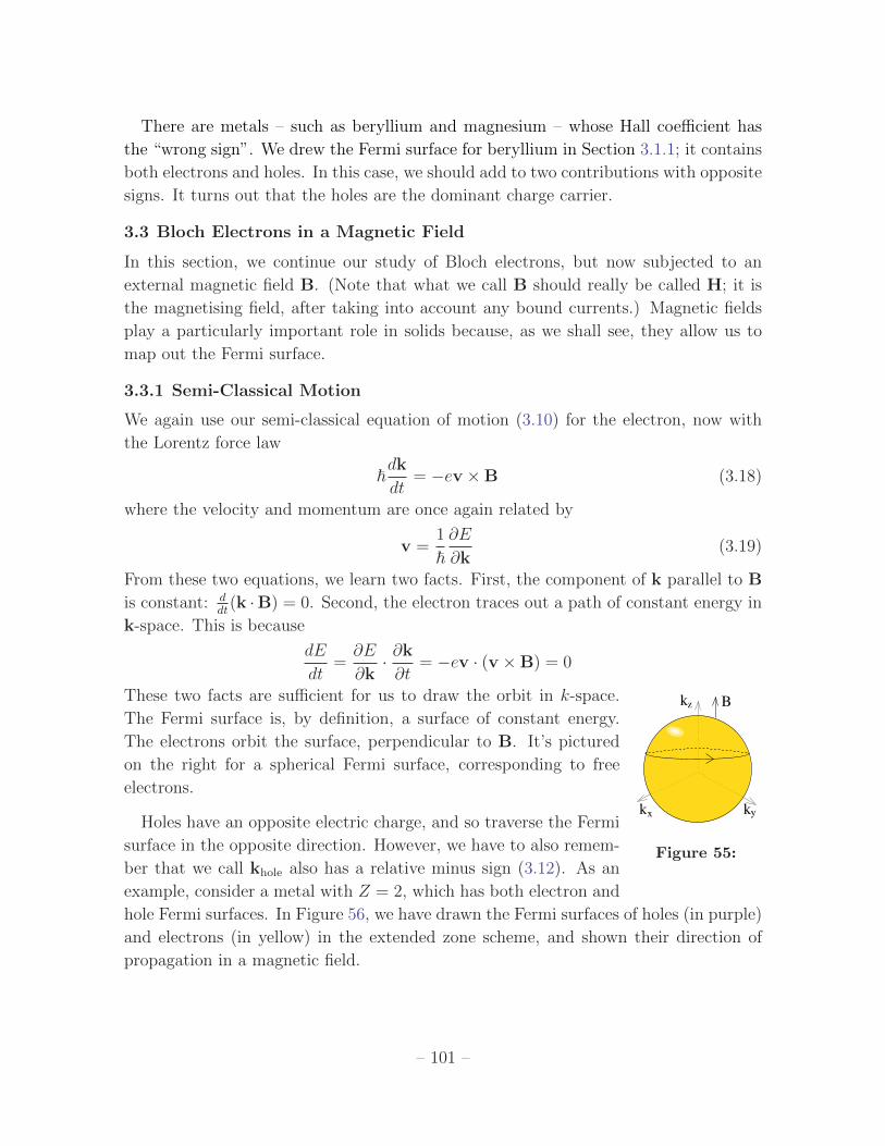
There are metals – such as beryllium and magnesium – whose Hall coefficient has

the “wrong sign”. We drew the Fermi surface for beryllium in Section 3.1.1; it contains

both electrons and holes. In this case, we should add to two contributions with opposite

signs. It turns out that the holes are the dominant charge carrier.

3.3 Bloch Electrons in a Magnetic Field

In this section, we continue our study of Bloch electrons, but now subjected to an

external magnetic field B. (Note that what we call B should really be called H; it is

the magnetising field, after taking into account any bound currents.) Magnetic fields

play a particularly important role in solids because, as we shall see, they allow us to

map out the Fermi surface.

3.3.1 Semi-Classical Motion

We again use our semi-classical equation of motion (3.10) for the electron, now with

the Lorentz force law

~dk

dt= −ev ×B (3.18)

where the velocity and momentum are once again related by

v =1

~∂E

∂k(3.19)

From these two equations, we learn two facts. First, the component of k parallel to B

is constant: ddt

(k ·B) = 0. Second, the electron traces out a path of constant energy in

k-space. This is because

dE

dt=∂E

∂k· ∂k

∂t= −ev · (v ×B) = 0

These two facts are sufficient for us to draw the orbit in k-space.

kk yx

kz B

Figure 55:

The Fermi surface is, by definition, a surface of constant energy.

The electrons orbit the surface, perpendicular to B. It’s pictured

on the right for a spherical Fermi surface, corresponding to free

electrons.

Holes have an opposite electric charge, and so traverse the Fermi

surface in the opposite direction. However, we have to also remem-

ber that we call khole also has a relative minus sign (3.12). As an

example, consider a metal with Z = 2, which has both electron and

hole Fermi surfaces. In Figure 56, we have drawn the Fermi surfaces of holes (in purple)

and electrons (in yellow) in the extended zone scheme, and shown their direction of

propagation in a magnetic field.

– 101 –

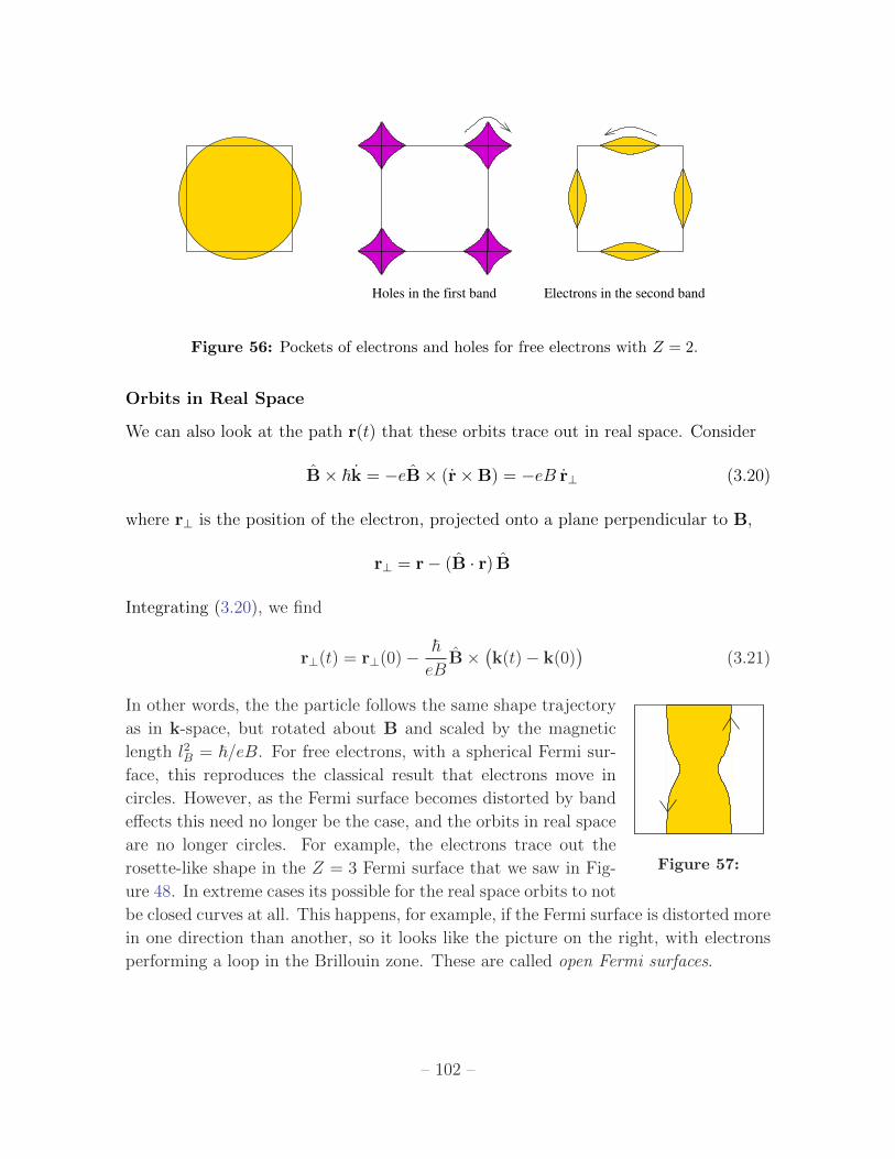
Holes in the first band Electrons in the second band

Figure 56: Pockets of electrons and holes for free electrons with Z = 2.

Orbits in Real Space

We can also look at the path r(t) that these orbits trace out in real space. Consider

B× ~k = −eB× (r×B) = −eB r⊥ (3.20)

where r⊥ is the position of the electron, projected onto a plane perpendicular to B,

r⊥ = r− (B · r) B

Integrating (3.20), we find

r⊥(t) = r⊥(0)− ~eB

B×(k(t)− k(0)

)(3.21)

In other words, the the particle follows the same shape trajectory

Figure 57:

as in k-space, but rotated about B and scaled by the magnetic

length l2B = ~/eB. For free electrons, with a spherical Fermi sur-

face, this reproduces the classical result that electrons move in

circles. However, as the Fermi surface becomes distorted by band

effects this need no longer be the case, and the orbits in real space

are no longer circles. For example, the electrons trace out the

rosette-like shape in the Z = 3 Fermi surface that we saw in Fig-

ure 48. In extreme cases its possible for the real space orbits to not

be closed curves at all. This happens, for example, if the Fermi surface is distorted more

in one direction than another, so it looks like the picture on the right, with electrons

performing a loop in the Brillouin zone. These are called open Fermi surfaces.

– 102 –

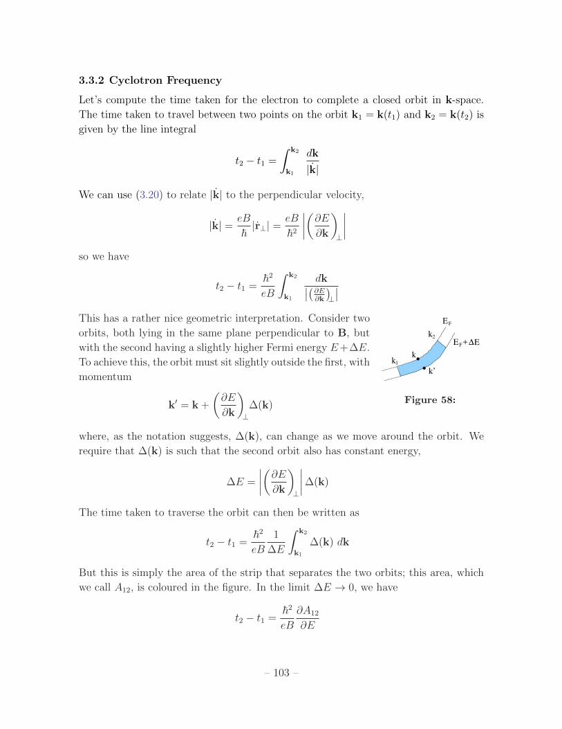
3.3.2 Cyclotron Frequency

Let’s compute the time taken for the electron to complete a closed orbit in k-space.

The time taken to travel between two points on the orbit k1 = k(t1) and k2 = k(t2) is

given by the line integral

t2 − t1 =

∫ k2

k1

dk

|k|

We can use (3.20) to relate |k| to the perpendicular velocity,

|k| = eB

~|r⊥| =

eB

~2

∣∣∣∣(∂E∂k

)⊥

∣∣∣∣so we have

t2 − t1 =~2

eB

∫ k2

k1

dk∣∣(∂E∂k

)⊥

∣∣This has a rather nice geometric interpretation. Consider two

F ∆EE +

EF

k1

k

k’

k2

Figure 58:

orbits, both lying in the same plane perpendicular to B, but

with the second having a slightly higher Fermi energy E+∆E.

To achieve this, the orbit must sit slightly outside the first, with

momentum

k′ = k +

(∂E

∂k

)⊥

∆(k)

where, as the notation suggests, ∆(k), can change as we move around the orbit. We

require that ∆(k) is such that the second orbit also has constant energy,

∆E =

∣∣∣∣(∂E∂k

)⊥

∣∣∣∣∆(k)

The time taken to traverse the orbit can then be written as

t2 − t1 =~2

eB

1

∆E

∫ k2

k1

∆(k) dk

But this is simply the area of the strip that separates the two orbits; this area, which

we call A12, is coloured in the figure. In the limit ∆E → 0, we have

t2 − t1 =~2

eB

∂A12

∂E

– 103 –

We can now apply this formula to compute the time taken to complete a closed orbit.

Let A(E) denote the area enclosed by the orbit. (Note that this will depend not only

on E but also on the component of the momentum k ·B parallel to the magnetic field.)

The time taken to complete an orbit is

T =~2

eB

∂A(E)

∂EThe cyclotron frequency is defined as

ωc =2π

T(3.22)

One can check that the cyclotron frequency agrees with the usual result, ωB = eB/m

for free electrons.

The fact that the cyclotron frequency ωc depends on some property of the Fermi

surface – namely ∂A/∂E – is important because the cyclotron frequency is something

that can be measured in experiments, since the electrons sit at resonance to absorb

microwaves tuned to the same frequency. This gives us our first hint as to how we

might measure properties of the Fermi surface.

3.3.3 Onsager-Bohr-Sommerfeld Quantisation

The combination of magnetic fields and Fermi surfaces gives rise to a host of further

physics but to see this we will have to work a little harder.

The heart of the problem is that, in classical physics, the Lorentz force does no

work. In the Hamiltonian formalism, this translates into the statement that the energy

does not depend on B when written in terms of the canonical momenta. Whenever

the energetics of a system depend on the magnetic field, there must be some quantum

mechanics going on underneath. In the present case, this means that we need to go

slightly beyond the simple semi-classical description that we’ve met above, to find some

of the discreteness that quantum mechanics introduces into the problem.

(As an aside: this problem is embodied in the Bohr-van-Leeuwen theorem, which

states that there can be no classical magnetism. We describe how quantum mechan-

ics can circumvent this in the discussion of Landau diamagnetism in the lectures on

Statistical Physics.)

To proceed, we would ideally like to quantise electrons in the presence of both a lattice

and a magnetic field. This is hard. We’ve learned how to quantise in the presence of

a magnetic field in Section 1 and in the presence of lattice in Section 2, but including

both turns out to be a much more difficult problem. Nonetheless, as we now show,

there’s a way to cobble together an approximation solution.

– 104 –

This cobbled-together quantisation was first proposed by Onsager, but follows an

earlier pre-quantum quantisation of Bohr and Sommerfield which suggests that, in any

system, an approximation to the quantisation of energy levels can be found by setting

1

2π

∮p · dr = ~(n+ γ) (3.23)

with n ∈ Z and γ an arbitrary constant. This Bohr-Sommerfeld quantisation does not,

in general, agree with the exact result from solving the Schrodinger equation. However,

it tends to capture the correct physics for large n, where the system goes over to its

semi-classical description.

In the present context, we apply Bohr-Sommerfeld quantisation to our semi-classical

model (3.18) and (3.19). We have

1

2π

∮p · dr =

~2π

∮k · dr =

~2

2πeB

∮k · (dk× B)

where, in the last equality, we have used our result (3.20). But this integral simply

captures the cross-sectional area of the orbit in k-space. This is the area A(E) that

we met above. We learn that the Bohr-Sommerfeld quantisation condition (3.23) leads

to a quantisation of the cross-sectional areas of the Fermi surface in the presence of a

magnetic field,

An =2πeB

~(n+ γ) (3.24)

This quantisation of area is actually a variant of the Landau level quantisation that we

met in Section 1.2. There are different ways of seeing this. First, note that, for fixed

kz, we can write the cyclotron frequency (3.22) as the difference between consecutive

energy levels

ωc =2πeB

~2

En+1 − EnAn+1 − An

=En+1 − En

~

Rearranging, this gives

En = ~ωc(n+ constant)

which coincides with our Landau level spectrum (1.14), except that the old cyclotron

frequency ωB = eB/m has been replaced by ωc.

– 105 –

Alternatively, we could look at the quantisation of area in real space, rather than in

k-space. We saw in (3.21), that the orbit in real space has the same shape as that in

k-space, but is scaled by a factor of l2B = ~/eB. This means that the flux through any

such orbit is given by

Φn =

(~eB

)2

BAn = (n+ γ)Φ0 (3.25)

where Φ0 = 2π~/e is the so-called quantum of flux. But this ties in nicely with our

discussion in Section 1.2 of Landau levels in the absence of a lattice, where we saw that

the degeneracy of states in each level is (1.17)

Β

Figure 59:

N =Φ

Φ0

which should clearly be an integer.

The quantisation (3.24) due to a background magnetic field

results in a re-arrangement of the Fermi surface, which now sit

in Landau tubes whose areas are quantised. A typical example

is shown on the right.

3.3.4 Quantum Oscillations

The formation of Landau tubes gives rise to a number of fairly striking experimental

signatures.

Consider a Fermi surface with energy EF and a second surface slightly inside with

energy EF − dE. The region between these contains the accessible states if we probe

the system with a small amount of energy dE. Now consider a Landau tube of cross-

sectional area An, intersecting our Fermi surface. Typically, the Landau tube will

intersect the Fermi surface only in some small region, as shown in left-hand picture

of Figure 60. This means that the number of states that can contribute to physical

processes will be fairly small. In the language that we introduced in the Statistical

Physics lectures, the density of states g(EF )dE within this Landau tube will be small.

However, something special happens if the area An happens to coincide with an

extremal area of the Fermi surface. Because the Fermi surface curves much more

slowly at such points, the density of states g(EF )dE is greatly enhanced at this point.

This is shown in the right-hand picture of Figure 60. In fact, one can show that the

density of states actually diverges at this point as g(E) ∼ (E − E?)−1/2.

– 106 –

Β Β

Figure 60: Landau tubes intersecting the Fermi surface: when the area of the tube coincides

with an extremal cross-section of the Fermi surface, there is a large enhancement in the

available states.

We learn that when the area quantisation takes special values, there are many more

electrons that can contribute to any physical process. However, the area quantisation

condition (3.24) changes with the magnetic field. This means that as we increase the

magnetic field, the areas of Landau tubes will increase and will, occasionally, overlap

with an extremal area in the Fermi surface. Indeed, if we denote the extremal cross-

sectional area of the Fermi surface as Aext, we must get an enhancement in the density

of available states whenever

An =2πeB

~(n+ γ) = Aext

for some n. We don’t know what γ is, but this doesn’t matter: the density of states

should occur over and over again, at intervals given by

∆

(1

B

)=

2πe

~1

Aext

Such oscillations are seen in a wide variety of physical measurements and go by the

collective name of quantum oscillations.

The first, and most prominent example of quantum oscillation is the de Haas-van

Alphen effect, in which the magnetisation M = −∂F/∂B varies with magnetic field.

The experimental data for gold is shown in the Figure5 61. Note that there are two

oscillation frequencies visible in the data. The Fermi surface of gold is shown on the

5The data is taken from I.M.Templeton, Proceedings of the Royal Society A, vol 292 (1965). Note

the old school graph paper.

– 107 –

Figure 61: dHvA oscillations for gold. The horizontal axis is B, plotted in kG.

right. For the oscillations above, the magnetic field is parallel to the neck of the Fermi

surface, as shown in the figure. The two frequencies then arise because there are two

extremal cross-sections – the neck and the belly. As the direction of the magnetic field

is changed, different extremal cross-sections become relevant. In this way, we can map

out the entire Fermi surface.

The magnetisation is not the only quantity to exhibit os-

Figure 62: Gold

cillations. In fact, the large enhancement in the density of states

affects nearly all observables. For example, oscillations in the

conductivity are known as the Shubikov-de Haas effect.

The experimental technique for measuring Fermi surfaces was

pioneered by Brian Pippard, Cavendish professor and the first

president of Clare Hall. Today, the techniques of quantum oscil-

lations play an important role in attempts to better understand

some of the more mysterious materials, such as unconventional

superconductors.

– 108 –

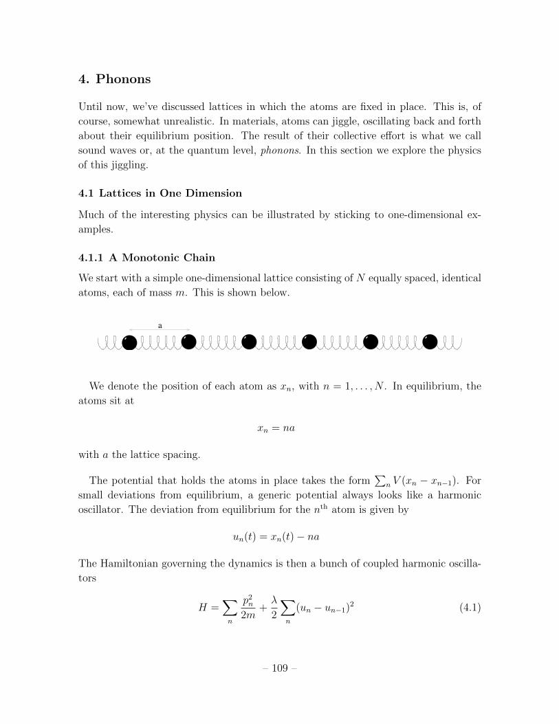
4. Phonons

Until now, we’ve discussed lattices in which the atoms are fixed in place. This is, of

course, somewhat unrealistic. In materials, atoms can jiggle, oscillating back and forth

about their equilibrium position. The result of their collective effort is what we call

sound waves or, at the quantum level, phonons. In this section we explore the physics

of this jiggling.

4.1 Lattices in One Dimension

Much of the interesting physics can be illustrated by sticking to one-dimensional ex-

amples.

4.1.1 A Monotonic Chain

We start with a simple one-dimensional lattice consisting of N equally spaced, identical

atoms, each of mass m. This is shown below.

a

We denote the position of each atom as xn, with n = 1, . . . , N . In equilibrium, the

atoms sit at

xn = na

with a the lattice spacing.

The potential that holds the atoms in place takes the form∑

n V (xn − xn−1). For

small deviations from equilibrium, a generic potential always looks like a harmonic

oscillator. The deviation from equilibrium for the nth atom is given by

un(t) = xn(t)− na

The Hamiltonian governing the dynamics is then a bunch of coupled harmonic oscilla-

tors

H =∑n

p2n

2m+λ

2

∑n

(un − un−1)2 (4.1)

– 109 –

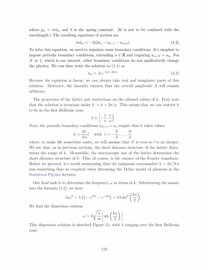
where pn = mun and λ is the spring constant. (It is not to be confused with the

wavelength.) The resulting equations of motion are

mun = −λ(2un − un−1 − un+1) (4.2)

To solve this equation, we need to stipulate some boundary conditions. It’s simplest to

impose periodic boundary conditions, extending n ∈ Z and requiring un+N = un. For

N 1, which is our interest, other boundary conditions do not qualitatively change

the physics. We can then write the solution to (4.2) as

un = Ae−iωt−ikna (4.3)

Because the equation is linear, we can always take real and imaginary parts of this

solution. Moreover, the linearity ensures that the overall amplitude A will remain

arbitrary.

The properties of the lattice put restrictions on the allowed values of k. First note

that the solution is invariant under k → k + 2π/a. This means that we can restrict k

to lie in the first Brillouin zone,

k ∈[−πa,π

a

)Next, the periodic boundary conditions uN+1 = u1 require that k takes values

k =2π

Nal with l = −N

2, . . . ,

N

2where, to make life somewhat easier, we will assume that N is even so l is an integer.

We see that, as in previous sections, the short distance structure of the lattice deter-

mines the range of k. Meanwhile, the macroscopic size of the lattice determines the

short distance structure of k. This, of course, is the essence of the Fourier transform.

Before we proceed, it’s worth mentioning that the minimum wavenumber k = 2π/Na

was something that we required when discussing the Debye model of phonons in the

Statistical Physics lectures.

Our final task is to determine the frequency ω in terms of k. Substituting the ansatz

into the formula (4.2), we have

mω2 = λ(2− eika − e−ika

)= 4λ sin2

(ka

2

)We find the dispersion relation

ω = 2

√λ

m

∣∣∣∣ sin(ka2) ∣∣∣∣

This dispersion relation is sketched Figure 63, with k ranging over the first Brillouin

zone.

– 110 –

π/a−π/a

ω (k)

k

Figure 63: Phonon dispersion relation for a monatomic chain.

Many aspects of the above discussion are familiar from the discussion of electrons in

the tight-binding model. In both cases, we end up with a dispersion relation over the

Brillouin zone. But there are some important differences. In particular, at small values

of k, the dispersion relation for phonons is linear

ω ≈√λ

mak

This is in contrast to the electron propagation where we get the dispersion relation for

a non-relativistic, massive particle (2.6). Instead, the dispersion relation for phonons is

more reminiscent of the massless, relativistic dispersion relation for light. For phonons,

the ripples travel with speed

cs =

√λ

ma (4.4)

This is the speed of sound in the material.

4.1.2 A Diatomic Chain

Consider now a linear chain of atoms, consisting of alternating atoms of different types.

a mass m mass M

The atoms on even sites have mass m; those on odd sites have mass M . For simplicity,

we’ll take the restoring forces between these atoms to be the same. The equations of

motion are

mu2n = −λ(2u2n − u2n−1 − u2n+1)

Mu2n+1 = −λ(2u2n+1 − u2n − u2n+2)

– 111 –

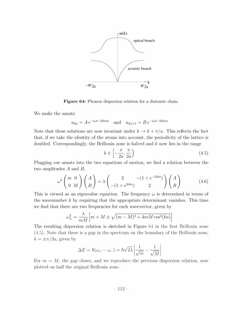
optical branch

acoustic branch

ω(k)

k−π/ π/2a2a

Figure 64: Phonon dispersion relation for a diatomic chain.

We make the ansatz

u2n = Ae−iωt−2ikna and u2n+1 = B e−iωt−2ikna

Note that these solutions are now invariant under k → k + π/a. This reflects the fact

that, if we take the identity of the atoms into account, the periodicity of the lattice is

doubled. Correspondingly, the Brillouin zone is halved and k now lies in the range

k ∈[− π

2a,π

2a

)(4.5)

Plugging our ansatz into the two equations of motion, we find a relation between the

two amplitudes A and B,

ω2

(m 0

0 M

)(A

B

)= λ

(2 −(1 + e−2ika)

−(1 + e2ika) 2

)(A

B

)(4.6)

This is viewed as an eigenvalue equation. The frequency ω is determined in terms of

the wavenumber k by requiring that the appropriate determinant vanishes. This time

we find that there are two frequencies for each wavevector, given by

ω2± =

λ

mM

[m+M ±

√(m−M)2 + 4mM cos2(ka)

]The resulting dispersion relation is sketched in Figure 64 in the first Brillouin zone

(4.5). Note that there is a gap in the spectrum on the boundary of the Brillouin zone,

k = ±π/2a, given by

∆E = ~(ω+ − ω−) = ~√

2λ

∣∣∣∣ 1√m− 1√

M

∣∣∣∣For m = M , the gap closes, and we reproduce the previous dispersion relation, now

plotted on half the original Brillouin zone.

– 112 –

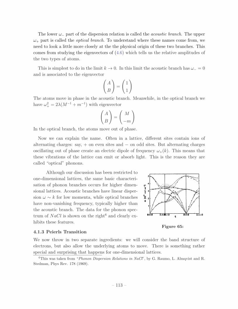
The lower ω− part of the dispersion relation is called the acoustic branch. The upper

ω+ part is called the optical branch. To understand where these names come from, we

need to look a little more closely at the the physical origin of these two branches. This

comes from studying the eigenvectors of (4.6) which tells us the relative amplitudes of

the two types of atoms.

This is simplest to do in the limit k → 0. In this limit the acoustic branch has ω− = 0

and is associated to the eigenvector(A

B

)=

(1

1

)The atoms move in phase in the acoustic branch. Meanwhile, in the optical branch we

have ω2+ = 2λ(M−1 +m−1) with eigenvector(

A

B

)=

(M

−m

)In the optical branch, the atoms move out of phase.

Now we can explain the name. Often in a lattice, different sites contain ions of

alternating charges: say, + on even sites and − on odd sites. But alternating charges

oscillating out of phase create an electric dipole of frequency ω+(k). This means that

these vibrations of the lattice can emit or absorb light. This is the reason they are

called “optical” phonons.

Although our discussion has been restricted to

Figure 65:

one-dimensional lattices, the same basic characteri-

sation of phonon branches occurs for higher dimen-

sional lattices. Acoustic branches have linear disper-

sion ω ∼ k for low momenta, while optical branches

have non-vanishing frequency, typically higher than

the acoustic branch. The data for the phonon spec-

trum of NaCl is shown on the right6 and clearly ex-

hibits these features.

4.1.3 Peierls Transition

We now throw in two separate ingredients: we will consider the band structure of

electrons, but also allow the underlying atoms to move. There is something rather

special and surprising that happens for one-dimensional lattices.6This was taken from “Phonon Dispersion Relations in NaCl”, by G. Raumo, L. Almqvist and R.

Stedman, Phys Rev. 178 (1969).

– 113 –

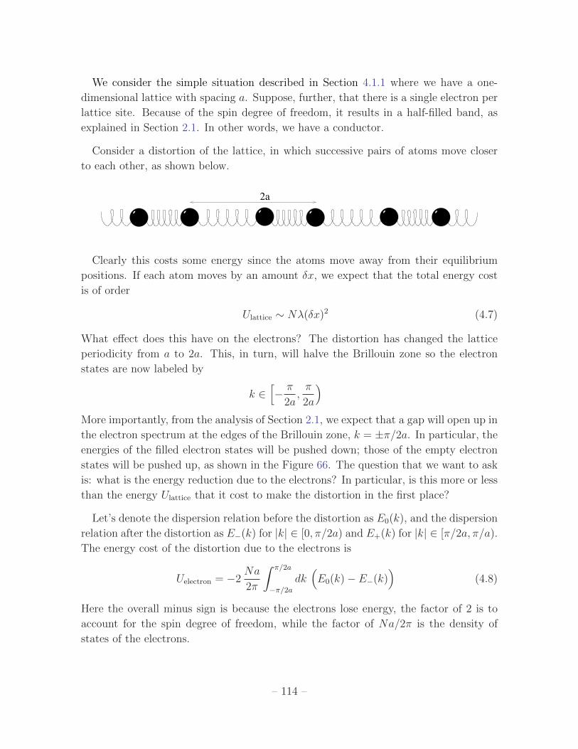
We consider the simple situation described in Section 4.1.1 where we have a one-

dimensional lattice with spacing a. Suppose, further, that there is a single electron per

lattice site. Because of the spin degree of freedom, it results in a half-filled band, as

explained in Section 2.1. In other words, we have a conductor.

Consider a distortion of the lattice, in which successive pairs of atoms move closer

to each other, as shown below.

2a

Clearly this costs some energy since the atoms move away from their equilibrium

positions. If each atom moves by an amount δx, we expect that the total energy cost

is of order

Ulattice ∼ Nλ(δx)2 (4.7)

What effect does this have on the electrons? The distortion has changed the lattice

periodicity from a to 2a. This, in turn, will halve the Brillouin zone so the electron

states are now labeled by

k ∈[− π

2a,π

2a

)More importantly, from the analysis of Section 2.1, we expect that a gap will open up in

the electron spectrum at the edges of the Brillouin zone, k = ±π/2a. In particular, the

energies of the filled electron states will be pushed down; those of the empty electron

states will be pushed up, as shown in the Figure 66. The question that we want to ask

is: what is the energy reduction due to the electrons? In particular, is this more or less

than the energy Ulattice that it cost to make the distortion in the first place?

Let’s denote the dispersion relation before the distortion as E0(k), and the dispersion

relation after the distortion as E−(k) for |k| ∈ [0, π/2a) and E+(k) for |k| ∈ [π/2a, π/a).

The energy cost of the distortion due to the electrons is

Uelectron = −2Na

2π

∫ π/2a

−π/2adk(E0(k)− E−(k)

)(4.8)

Here the overall minus sign is because the electrons lose energy, the factor of 2 is to

account for the spin degree of freedom, while the factor of Na/2π is the density of

states of the electrons.

– 114 –

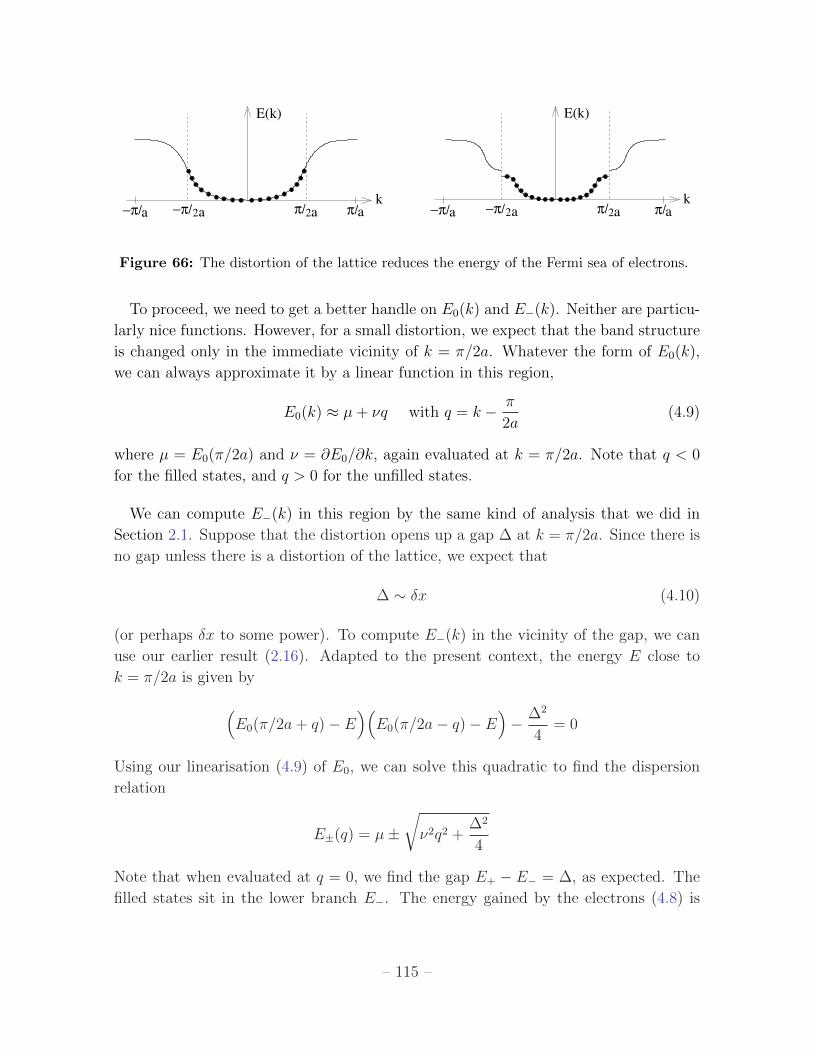
π/a−π/a −π/2a π/2aπ/2a π/a−π/a

E(k)

k−π/2a

E(k)

k

Figure 66: The distortion of the lattice reduces the energy of the Fermi sea of electrons.

To proceed, we need to get a better handle on E0(k) and E−(k). Neither are particu-

larly nice functions. However, for a small distortion, we expect that the band structure

is changed only in the immediate vicinity of k = π/2a. Whatever the form of E0(k),

we can always approximate it by a linear function in this region,

E0(k) ≈ µ+ νq with q = k − π

2a(4.9)

where µ = E0(π/2a) and ν = ∂E0/∂k, again evaluated at k = π/2a. Note that q < 0

for the filled states, and q > 0 for the unfilled states.

We can compute E−(k) in this region by the same kind of analysis that we did in

Section 2.1. Suppose that the distortion opens up a gap ∆ at k = π/2a. Since there is

no gap unless there is a distortion of the lattice, we expect that

∆ ∼ δx (4.10)

(or perhaps δx to some power). To compute E−(k) in the vicinity of the gap, we can

use our earlier result (2.16). Adapted to the present context, the energy E close to

k = π/2a is given by(E0(π/2a+ q)− E

)(E0(π/2a− q)− E

)− ∆2

4= 0

Using our linearisation (4.9) of E0, we can solve this quadratic to find the dispersion

relation

E±(q) = µ±√ν2q2 +

∆2

4

Note that when evaluated at q = 0, we find the gap E+ − E− = ∆, as expected. The

filled states sit in the lower branch E−. The energy gained by the electrons (4.8) is

– 115 –

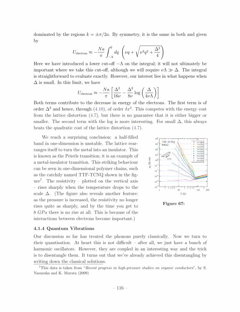
dominated by the regions k = ±π/2a. By symmetry, it is the same in both and given

by

Uelectron ≈ −Na

π

∫ 0

−Λ

dq

(νq +

√ν2q2 +

∆2

4

)Here we have introduced a lower cut-off −Λ on the integral; it will not ultimately be

important where we take this cut-off, although we will require νΛ ∆. The integral

is straightforward to evaluate exactly. However, our interest lies in what happens when

∆ is small. In this limit, we have

Uelectron ≈ −Na

π

[∆2

16ν− ∆2

8νlog

(∆

4νΛ

)]Both terms contribute to the decrease in energy of the electrons. The first term is of

order ∆2 and hence, through (4.10), of order δx2. This competes with the energy cost

from the lattice distortion (4.7), but there is no guarantee that it is either bigger or

smaller. The second term with the log is more interesting. For small ∆, this always

beats the quadratic cost of the lattice distortion (4.7).

We reach a surprising conclusion: a half-filled

Figure 67:

band in one-dimension is unstable. The lattice rear-

ranges itself to turn the metal into an insulator. This

is known as the Peierls transition; it is an example of

a metal-insulator transition. This striking behaviour

can be seen in one-dimensional polymer chains, such

as the catchily named TTF-TCNQ shown in the fig-

ure7. The resistivity – plotted on the vertical axis

– rises sharply when the temperature drops to the

scale ∆. (The figure also reveals another feature:

as the pressure is increased, the resistivity no longer

rises quite as sharply, and by the time you get to

8 GPa there is no rise at all. This is because of the

interactions between electrons become important.)

4.1.4 Quantum Vibrations

Our discussion so far has treated the phonons purely classically. Now we turn to

their quantisation. At heart this is not difficult – after all, we just have a bunch of

harmonic oscillators. However, they are coupled in an interesting way and the trick

is to disentangle them. It turns out that we’ve already achieved this disentangling by

writing down the classical solutions.7This data is taken from “Recent progress in high-pressure studies on organic conductors”, by S.

Yasuzuka and K. Murata (2009)

– 116 –

We have a classical solution (4.3) for each kl = 2πl/Na with l = −N/2, . . . , N/2.

We will call the corresponding frequency ωl = 2√λ/m| sin(kla/2)|. We can introduce a

different amplitude for each l. The most general classical solution then takes the form

un(t) = X0(t) +∑l 6=0

[αl e

−i(ωlt−klna) + α†l ei(ωlt−klna)

](4.11)

This requires some explanation. First, we sum over all modes l = −N/2, . . . ,+N/2with the exception of l = 0. This has been singled out and written as X0(t). It is

the centre of mass, reflecting the fact that the entire lattice can move as one. The

amplitudes for each l 6= 0 mode are denoted αl. Finally, we have taken the real part

of the solution because, ultimately, un(t) should be real. Note that we’ve denoted the

complex conjugation by α†l rather than α?l in anticipation of the quantisation that we

will turn to shortly.

The momentum pn(t) = mun is given by

pn(t) = P0(t) +∑l 6=0

[−imωlαl e−i(ωlt−klna) + imωlα

†l e

i(ωlt−klna)]

Now we turn to the quantum theory. We promote un and pn to operators acting on a

Hilbert space. We should think of un(t) and pn(t) as operators in the Heisenberg rep-

resentation; we can get the corresponding operators in the Schrodinger representation

simply by setting t = 0.

Since un and pn are operators, the amplitudes αl and α†l must also be operators if

we want these equations to continue to make sense. We can invert the equations above

by setting t = 0 and looking at

N∑n=1

un e−iklna =

∑n

∑l′

[αl′ e

−i(kl−kl′ )na + α†l′ e−i(kl+kl′ )na

]= N(αl + α†−l)

Similarly,

N∑n=1

pn eiklna =

∑n

∑l′

[−imωl′αl′ e−i(kl−kl′ )na + imωl′α

†l′ e−i(kl+kl′ )na

]= −iNmωl(αl − α†−l)

where we’ve used the fact that ωl = ω−l. We can invert these equations to find

αl =1

2mωlN

∑n

e−iklna(mωlun + ipn

)α†l =

1

2mωlN

∑n

eiklna(mωlun − ipn

)(4.12)

– 117 –

Similarly, we can write the centre of mass coordinates — which are also now operators

— as

X0 =1

N

∑n

un and P0 =1

N

∑n

pn (4.13)

At this point, we’re ready to turn to the commutation relations. The position and

momentum of each atom satisfy

[un, pn′ ] = i~δn,n′

A short calculation using the expressions above reveals that X0 and P0 obey the rela-

tions

[X0, P0] =i~N

Meanwhile, the amplitudes obey the commutation relations

[αl, α†l′ ] =

~2mωlN

δl,l′ and [αl, αl′ ] = [α†l , α†l′ ] = 0

This is something that we’ve seen before: they are simply the creation and annihilation

operators of a simple harmonic oscillator. We rescale

αl =

√~

2mωlNal (4.14)

then our new operators al obey

[al, a†l′ ] = δl,l′ and [al, al′ ] = [a†l , a

†l′ ] = 0

Phonons

We now turn to the Hamiltonian (4.1). Substituting in our expressions (4.12) and

(4.13), and after a bit of tedious algebra, we find the Hamiltonian

H =P 2

0

2M+∑l 6=0

(a†lal +

1

2

)~ωl

Here M = Nm is the mass of the entire lattice. Since this is a macroscopically large

object, we set P0 = 0 and focus on the Hilbert space arising from the creation operators

a†l . After our manipulations, these are simply N , decoupled harmonic oscillators.

– 118 –

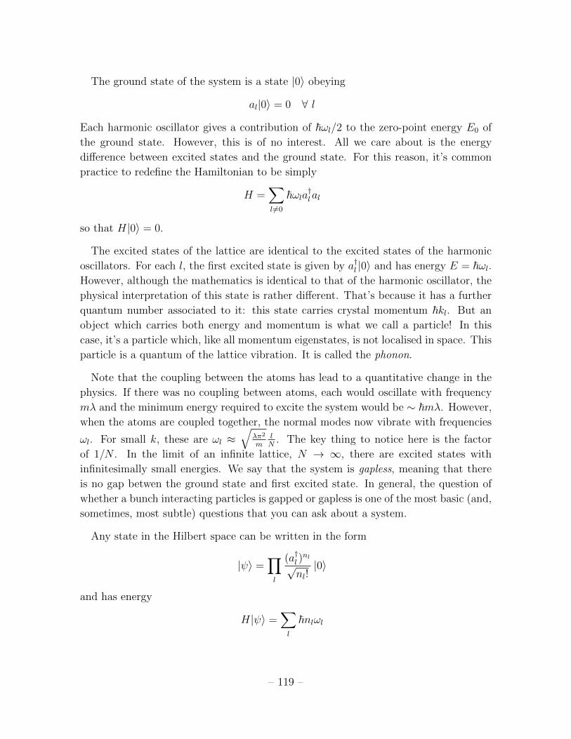
The ground state of the system is a state |0〉 obeying

al|0〉 = 0 ∀ l

Each harmonic oscillator gives a contribution of ~ωl/2 to the zero-point energy E0 of

the ground state. However, this is of no interest. All we care about is the energy

difference between excited states and the ground state. For this reason, it’s common

practice to redefine the Hamiltonian to be simply

H =∑l 6=0

~ωla†lal

so that H|0〉 = 0.

The excited states of the lattice are identical to the excited states of the harmonic

oscillators. For each l, the first excited state is given by a†l |0〉 and has energy E = ~ωl.However, although the mathematics is identical to that of the harmonic oscillator, the

physical interpretation of this state is rather different. That’s because it has a further

quantum number associated to it: this state carries crystal momentum ~kl. But an

object which carries both energy and momentum is what we call a particle! In this

case, it’s a particle which, like all momentum eigenstates, is not localised in space. This

particle is a quantum of the lattice vibration. It is called the phonon.

Note that the coupling between the atoms has lead to a quantitative change in the

physics. If there was no coupling between atoms, each would oscillate with frequency

mλ and the minimum energy required to excite the system would be ∼ ~mλ. However,

when the atoms are coupled together, the normal modes now vibrate with frequencies

ωl. For small k, these are ωl ≈√

λπ2

mlN

. The key thing to notice here is the factor

of 1/N . In the limit of an infinite lattice, N → ∞, there are excited states with

infinitesimally small energies. We say that the system is gapless, meaning that there

is no gap betwen the ground state and first excited state. In general, the question of

whether a bunch interacting particles is gapped or gapless is one of the most basic (and,

sometimes, most subtle) questions that you can ask about a system.

Any state in the Hilbert space can be written in the form

|ψ〉 =∏l

(a†l )nl

√nl!|0〉

and has energy

H|ψ〉 =∑l

~nlωl

– 119 –

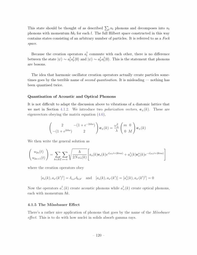
This state should be thought of as described∑

l nl phonons and decomposes into nlphonons with momentum ~kl for each l. The full Hilbert space constructed in this way

contains states consisting of an arbitrary number of particles. It is referred to as a Fock

space.

Because the creation operators a†l commute with each other, there is no difference

between the state |ψ〉 ∼ a†la†l′ |0〉 and |ψ〉 ∼ a†l′a

†l |0〉. This is the statement that phonons

are bosons.

The idea that harmonic oscillator creation operators actually create particles some-

times goes by the terrible name of second quantisation. It is misleading — nothing has

been quantised twice.

Quantisation of Acoustic and Optical Phonons

It is not difficult to adapt the discussion above to vibrations of a diatomic lattice that

we met in Section 4.1.2. We introduce two polarization vectors, e±(k). These are

eigenvectors obeying the matrix equation (4.6),(2 −(1 + e−2ika)

−(1 + e2ika) 2

)e±(k) =

ω2±

λ

(m 0

0 M

)e±(k)

We then write the general solution as(u2n(t)

u2n+1(t)

)=∑k∈BZ

∑s=±

√~

2Nωs(k)

[as(k)es(k)ei(ωst+2kna) + a†s(k)e?s(k)e−i(ωst+2kna)

]

where the creation operators obey

[as(k), as′(k′)†] = δs,s′δk,k′ and [as(k), as′(k

′)] = [a†s(k), as′(k′)†] = 0

Now the operators a†−(k) create acoustic phonons while a†+(k) create optical phonons,

each with momentum ~k.

4.1.5 The Mossbauer Effect

There’s a rather nice application of phonons that goes by the name of the Mossbauer

effect. This is to do with how nuclei in solids absorb gamma rays.

– 120 –

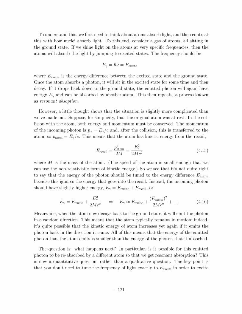
To understand this, we first need to think about atoms absorb light, and then contrast

this with how nuclei absorb light. To this end, consider a gas of atoms, all sitting in

the ground state. If we shine light on the atoms at very specific frequencies, then the

atoms will absorb the light by jumping to excited states. The frequency should be

Eγ = ~ν = Eexcite

where Eexcite is the energy difference between the excited state and the ground state.

Once the atom absorbs a photon, it will sit in the excited state for some time and then

decay. If it drops back down to the ground state, the emitted photon will again have

energy Eγ and can be absorbed by another atom. This then repeats, a process known

as resonant absoption.

However, a little thought shows that the situation is slightly more complicated than

we’ve made out. Suppose, for simplicity, that the original atom was at rest. In the col-

lision with the atom, both energy and momentum must be conserved. The momentum

of the incoming photon is pγ = Eγ/c and, after the collision, this is transferred to the

atom, so patom = Eγ/c. This means that the atom has kinetic energy from the recoil,

Erecoil =p2

atom

2M=

E2γ

2Mc2(4.15)

where M is the mass of the atom. (The speed of the atom is small enough that we

can use the non-relativistic form of kinetic energy.) So we see that it’s not quite right

to say that the energy of the photon should be tuned to the energy difference Eexcite

because this ignores the energy that goes into the recoil. Instead, the incoming photon

should have slightly higher energy, Eγ = Eexcite + Erecoil, or

Eγ = Eexcite +E2γ

2Mc2⇒ Eγ ≈ Eexcite +

(Eexcite)2

2Mc2+ . . . (4.16)

Meanwhile, when the atom now decays back to the ground state, it will emit the photon

in a random direction. This means that the atom typically remains in motion; indeed,

it’s quite possible that the kinetic energy of atom increases yet again if it emits the

photon back in the direction it came. All of this means that the energy of the emitted

photon that the atom emits is smaller than the energy of the photon that it absorbed.

The question is: what happens next? In particular, is it possible for this emitted

photon to be re-absorbed by a different atom so that we get resonant absorption? This

is now a quantitative question, rather than a qualitative question. The key point is

that you don’t need to tune the frequency of light exactly to Eexcite in order to excite

– 121 –

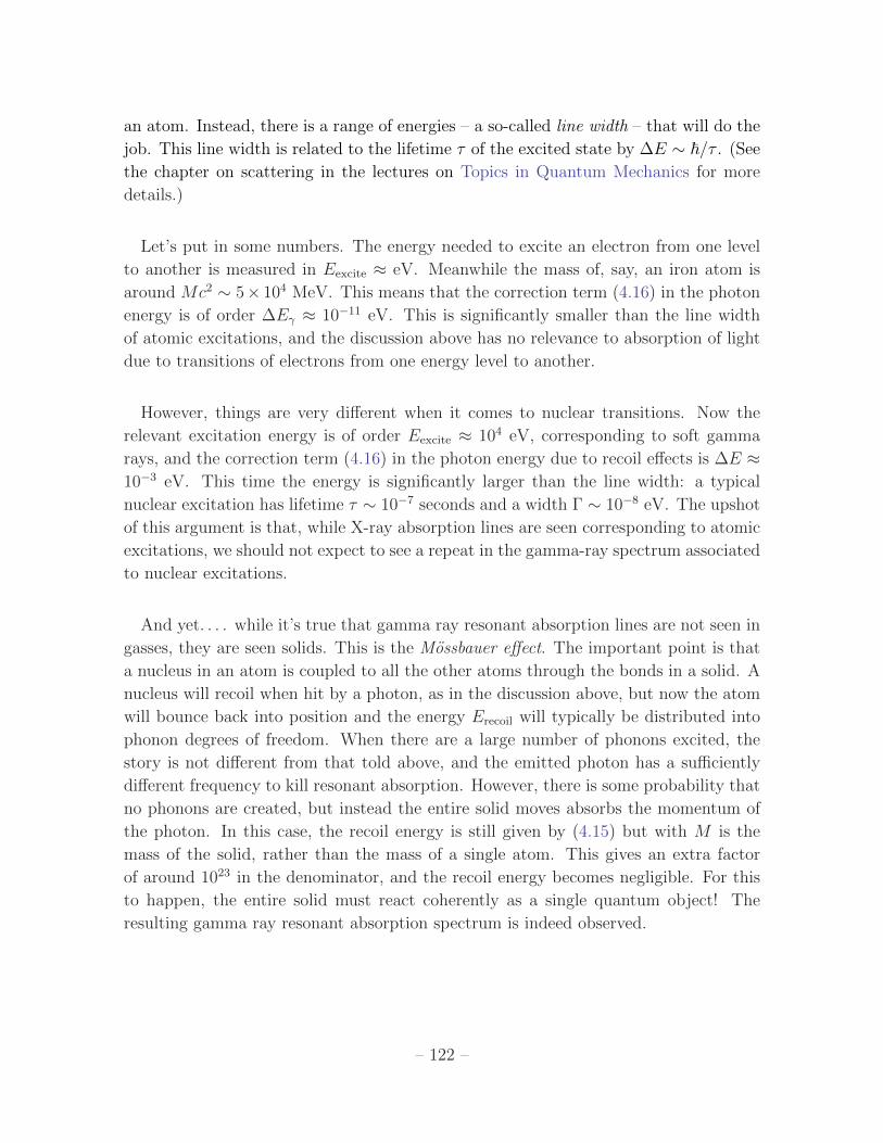
an atom. Instead, there is a range of energies – a so-called line width – that will do the

job. This line width is related to the lifetime τ of the excited state by ∆E ∼ ~/τ . (See

the chapter on scattering in the lectures on Topics in Quantum Mechanics for more

details.)

Let’s put in some numbers. The energy needed to excite an electron from one level

to another is measured in Eexcite ≈ eV. Meanwhile the mass of, say, an iron atom is

around Mc2 ∼ 5× 104 MeV. This means that the correction term (4.16) in the photon

energy is of order ∆Eγ ≈ 10−11 eV. This is significantly smaller than the line width

of atomic excitations, and the discussion above has no relevance to absorption of light

due to transitions of electrons from one energy level to another.

However, things are very different when it comes to nuclear transitions. Now the

relevant excitation energy is of order Eexcite ≈ 104 eV, corresponding to soft gamma

rays, and the correction term (4.16) in the photon energy due to recoil effects is ∆E ≈10−3 eV. This time the energy is significantly larger than the line width: a typical

nuclear excitation has lifetime τ ∼ 10−7 seconds and a width Γ ∼ 10−8 eV. The upshot

of this argument is that, while X-ray absorption lines are seen corresponding to atomic

excitations, we should not expect to see a repeat in the gamma-ray spectrum associated

to nuclear excitations.

And yet. . . . while it’s true that gamma ray resonant absorption lines are not seen in

gasses, they are seen solids. This is the Mossbauer effect. The important point is that

a nucleus in an atom is coupled to all the other atoms through the bonds in a solid. A

nucleus will recoil when hit by a photon, as in the discussion above, but now the atom

will bounce back into position and the energy Erecoil will typically be distributed into

phonon degrees of freedom. When there are a large number of phonons excited, the

story is not different from that told above, and the emitted photon has a sufficiently

different frequency to kill resonant absorption. However, there is some probability that

no phonons are created, but instead the entire solid moves absorbs the momentum of

the photon. In this case, the recoil energy is still given by (4.15) but with M is the

mass of the solid, rather than the mass of a single atom. This gives an extra factor

of around 1023 in the denominator, and the recoil energy becomes negligible. For this

to happen, the entire solid must react coherently as a single quantum object! The

resulting gamma ray resonant absorption spectrum is indeed observed.

– 122 –

4.2 From Atoms to Fields

If we look at a solid at suitably macroscopic distances, we don’t notice the underlying

atomic structure. Nonetheless, it’s still straightforward to detect sound waves. This

suggests that we should be able to formulate a continuum description of the solid that

is ignorant of the underlying atomic make-up.

With this in mind, we define the displacement field for a one-dimensional lattice.

This is a function u(x, t). It is initially defined only at the lattice points

u(x = na) = un

However, we then extend this field to all x ∈ R, with the proviso that our theory will

cease to make sense if u(x) varies appreciably on scales smaller than a.

The equation governing the atomic displacements is (4.2)

mun = −λ(2un − un−1 − un+1)

In the continuum limit, this difference equation becomes the wave equation

ρ∂2u

∂t2= −λ′ ∂

2u

∂x2(4.17)

where ρ = m/a is the density of our one-dimensional solid, and λ′ = λa. These are

the macroscopic parameters. Note, in particular, that the speed of sound (4.4) can be

written purely in terms of these macroscopic parameters, c2s = λ′/ρ.

The equation of motion (4.17) can be derived from the action

S =

∫dtdx

[ρ

2

(∂u

∂t

)2

− λ′

2

(∂u

∂x

)2]

This is the field theory for the phonons of a one-dimensional solid.

4.2.1 Phonons in Three Dimensions

For three-dimensional solids, there are three displacement fields, ui(x), one for each

direction in which the lattice can deform. In general, the resulting action can depend

on various quantities ∂ui/∂xj. However, if the underlying lattice is such that the long-

wavelength dynamics is rotationally invariant, then the action can only be a function

of the symmetric combination

uij =1

2

(∂ui∂xj

+∂uj∂xi

)

– 123 –

If we want an equation of motion linear in the displacement, then the most general

action is a function of uijuij or u2kk. (The term ukk is a total derivative and does not

affect the equation of motion). We have

S =

∫dtd3x

1

2

[ρ

(∂ui∂t

)2

− 2µuijuij − λuiiujj

](4.18)

The coefficients µ and λ are called Lame coeffcients; they characterise the underlying

solid.

This action gives rise to the equations of motion

ρ∂2ui∂t2

= (µ+ λ)∂2uj∂xi∂xj

+ µ∂2ui∂xj∂xj

(4.19)

We can look for solutions of the form

ui(x, t) = εi ei(k·x+ωt)

where εi determines the polarisation of the wave. Plugging this ansatz into the equation

of motion gives us the relation

ρω2εi = µk2εi + (µ+ λ)(ε · k)ki

The frequency of the wave depends on the polarisation. There are two different options.

Longitudinal waves have k ∼ ε. These have dispersion

ω2 =2µ+ λ

ρk2 (4.20)

Meanwhile, transverse waves have ε · k = 0 and dispersion

ω2 =µ

ρk2 (4.21)

Note that both of these dispersion relations are linear. The continuum approximation

only captures the low-k limit of the full lattice system and does not see the bending

of the dispersion relation close to the edge of the Brillouin zone. This is because it is

valid only at long wavelengths, ka 1.

The general solution to (4.19) is then

ui(x, t) =∑s

∫d3k

(2π)3

1

2ρωs(k)εsi

(as(k) ei(k·x−ωst) + a†s(k) e−i(k·x−ωst)

)(4.22)

where the s sum is over the three polarisation vectors, two transverse and one longi-

tudinal. The frequencies ωs(k) correspond to either (4.20) or (4.21) depending on the

choice of s.

– 124 –

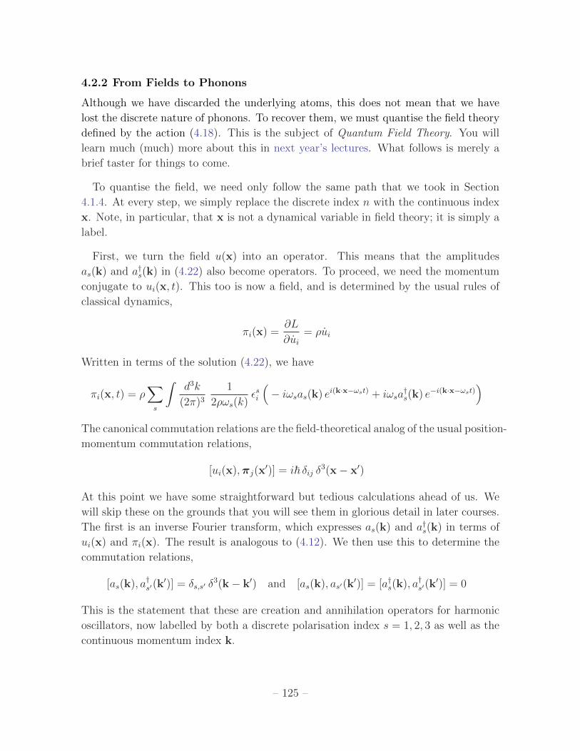
4.2.2 From Fields to Phonons

Although we have discarded the underlying atoms, this does not mean that we have

lost the discrete nature of phonons. To recover them, we must quantise the field theory

defined by the action (4.18). This is the subject of Quantum Field Theory. You will

learn much (much) more about this in next year’s lectures. What follows is merely a

brief taster for things to come.

To quantise the field, we need only follow the same path that we took in Section

4.1.4. At every step, we simply replace the discrete index n with the continuous index

x. Note, in particular, that x is not a dynamical variable in field theory; it is simply a

label.

First, we turn the field u(x) into an operator. This means that the amplitudes

as(k) and a†s(k) in (4.22) also become operators. To proceed, we need the momentum

conjugate to ui(x, t). This too is now a field, and is determined by the usual rules of

classical dynamics,

πi(x) =∂L

∂ui= ρui

Written in terms of the solution (4.22), we have

πi(x, t) = ρ∑s

∫d3k

(2π)3

1

2ρωs(k)εsi

(− iωsas(k) ei(k·x−ωst) + iωsa

†s(k) e−i(k·x−ωst)

)The canonical commutation relations are the field-theoretical analog of the usual position-

momentum commutation relations,

[ui(x),πj(x′)] = i~ δij δ3(x− x′)

At this point we have some straightforward but tedious calculations ahead of us. We

will skip these on the grounds that you will see them in glorious detail in later courses.

The first is an inverse Fourier transform, which expresses as(k) and a†s(k) in terms of

ui(x) and πi(x). The result is analogous to (4.12). We then use this to determine the

commutation relations,

[as(k), a†s′(k′)] = δs,s′ δ

3(k− k′) and [as(k), as′(k′)] = [a†s(k), a†s′(k

′)] = 0

This is the statement that these are creation and annihilation operators for harmonic

oscillators, now labelled by both a discrete polarisation index s = 1, 2, 3 as well as the

continuous momentum index k.

– 125 –

The next fairly tedious calculation is the Hamiltonian. This too follows from standard

rules of classical dynamics, together with a bunch of Fourier transforms. When the dust

settles, we find that, up to an irrelevant overall constant,

H =∑s

∫d3k

(2π)3~ωs(k)a†s(k)as(k)

This is simply the Hamiltonian for an infinite number of harmonic oscillators.

The interpretation is the same as we saw in Section 4.1.4. We define the ground

state of the field theory to obey as(k)|0〉 = 0 for all s and for all k. The Fourier modes

of the field a†s(k) are then to be viewed as creating and destroying phonons which

carry momentum ~k, polarisation εs and energy ~ωs(k). In this way, we see particles

emerging from an underlying field.

Lessons for the Future

This has been a very quick pass through some basic quantum field theory, applied to

the vibrations of the lattice. Buried within the mathematics of this section are two,

key physical ideas. The first is that a coarse grained description of atomic vibrations

can be described in terms of a continuous field. The second is that quantisation of the

field results in particles that, in the present context, we call phonons.

There is a very important lesson to take from the second of these ideas, a lesson

which extends well beyond the study of solids. All of the fundamental particles that

we know of in Nature – whether electrons, quarks, photons, or anything else — arise

from the quantisation of an underlying field. This is entirely analogous to the way that

phonons arose in the discussion above.

Is there also a lesson to take away from the first idea above? Could it be that the

fundamental fields of Nature themselves arise from coarse-graining something smaller?

The honest answer is that we don’t know. However, perhaps surprisingly, all signs point

towards this not being the case. First, and most importantly, there is no experimental

evidence that the fundamental fields in our Universe have a discrete underpinning. But

at the theoretical level, there are some deep mathematical reasons — to do with chiral

fermions and topology — which suggest that it is not possible to find a discrete system

from which the known laws of physics emerge. It would appear that our Universe

does not have something akin to the atomic lattice which underlies the phonon field.

Understanding these issues remains a vibrant topic of research, both in condensed

matter physics and in high energy physics.

– 126 –