Statistical Diagnosis for Intermittent Statistical Diagnosis for Intermittent Scan Chain Hold-Time FaultScan Chain Hold-Time Fault

Laboratory for Reliable Computing (LaRC)

Electrical Engineering Department

National Tsing Hua University

Yu Huang, Wu-Tung Cheng, S. M. Reddy,

Cheng-Ju Hsieh, Yu-Ting Hung

ITC 2003

2

ReferencesReferences [1] A Technique for Fault Diagnosis of Defects in Scan

ChainsRuifeng Guo, Srikanth Venkataraman ITC 2001

[2] Efficient Diagnosis for Multiple Intermittent Scan Chain Hold-Time Faults

Yu Huang, Wu-Tung Cheng, Cheng-Ju Hsieh ATS 2003

3

OutlineOutline Introduction

Fault Model

Hold-time faults

Upper bound and lower bound calculation

Statistical diagnosis algorithm

Experimental results

Conclusion

4

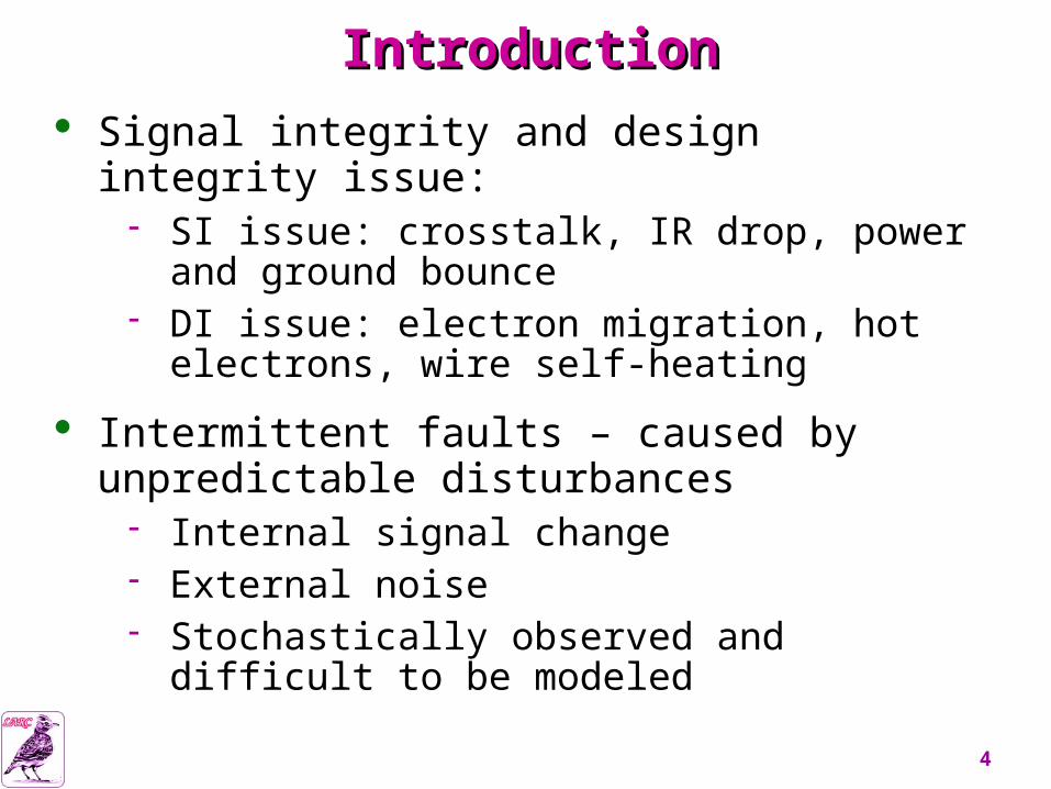
IntroductionIntroduction

Signal integrity and design integrity issue: SI issue: crosstalk, IR drop, power and ground

bounce DI issue: electron migration, hot electrons, wire

self-heating

Intermittent faults – caused by unpredictable disturbances

Internal signal change External noise Stochastically observed and difficult to be

modeled

5

IntroductionIntroduction Scan designs are susceptible to hold-time

violations

Wire delay is difficult to calculate accurately Inserted delay element for fixing hold time?

When the hold time margin is small, it may cause the hold-time error

Statistical diagnosis Permanent fault is a special type of intermittent

fault

6

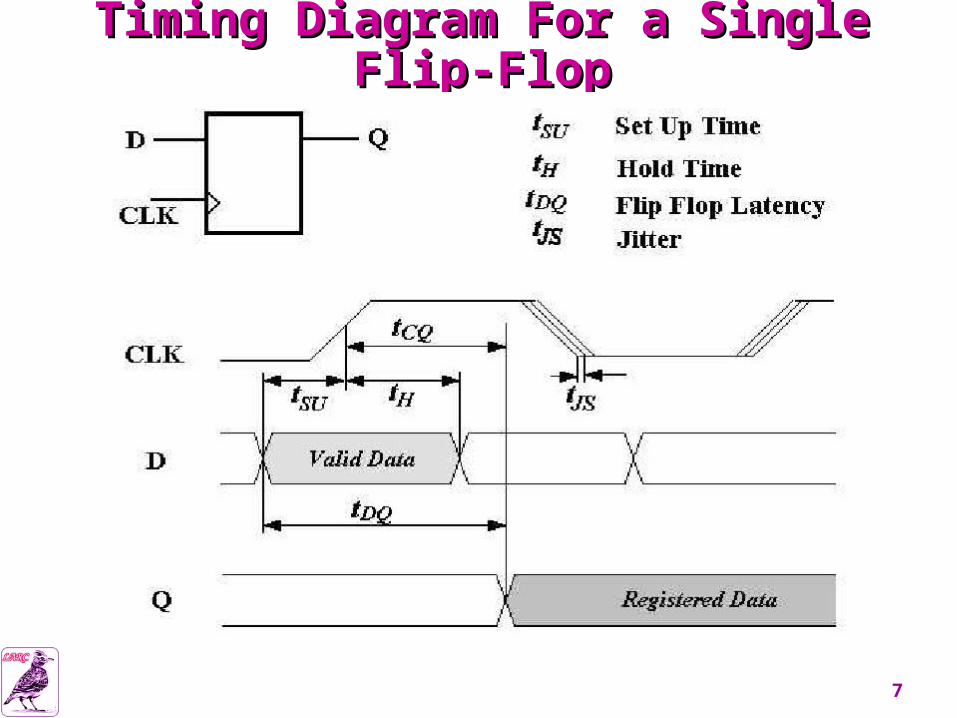
Fault model of Transition FaultsFault model of Transition Faults Slow-to-rise:

001100110011 → 00100010001X

Slow-to-fall:

001100110011 → 011101110111

Fast-to-rise:

001100110011 → X01110111011

Fast-to-fall:

001100110011 → 000100010001

7

Timing Diagram For a Single Flip-FlopTiming Diagram For a Single Flip-Flop

8

Timing Diagram For a Scan ChainTiming Diagram For a Scan Chain

td

9

Hold-Time Fault TypeHold-Time Fault Type Type-I: captures incorrect data iff a “0 → 1”

transition at the input of a faulty cell

Type-II: captures incorrect data iff a “1 → 0” transition at the input of a faulty cell

Type-III: Hold-time fault happens whenever there is a transition at the input of a faulty cell

10

Fault With Probably TriggeredFault With Probably Triggered Ex. Type-I hold time fault

110011001100 → 111011101110 or

110011101110

The fault is only triggered with a probability Prob.

The diagnosis of the faulty site may not point to the exact faulty scan cell

11

Assumption of Statistical Diagnosis AlgorithmAssumption of Statistical Diagnosis Algorithm

Use flush patterns to identify the faulty chains and fault types

Other types of scan chain faults can be diagnosed by this method with simple modification

The hold-time fault can only happen during the scan chain loading/unloading. The capture is fault-free

12

Upper Bound CalculationUpper Bound Calculation

1001011000110001

X10XXXXXXX10XXXX

Shift in

Capture

Shift out X11XXXXXXX10XXXX

X11XXXXXXX11XXXX

13

Set Constraint EffectivelySet Constraint Effectively Step 1: reduce the faulty masks of the candidate

set Based on flushing pattern responses Ex. The candidate set includes scan cells

(14,11,8,3) on the chain

Step 2: reduced the set by identifying scan cells impossibly to be corrupted Sub-Step 1: set “X” to scan cell s which is

impossibly to be corrupted EX. Load 100101100011X001 to the faulty scan

chain and perform logic simulation

14

Set Constraint EffectivelySet Constraint Effectively Sub-Step 2: All scan cells and POs that captured

“X”s are grouped into a set, say Gs ,all scan cells or POs in Gs should be observed to have failures for this pattern by tester (per pattern based total match condition)

Sub-Step 3: If more than one scan cells has corrupted values, it might produce fault masking. Observed correctly by the tester Multiple fan-in from faulty chains At least two of these fan-in from faulty chains have

sensitive transitions

15

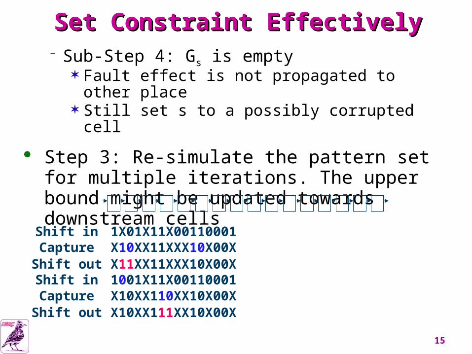
Set Constraint EffectivelySet Constraint Effectively Sub-Step 4: Gs is empty

Fault effect is not propagated to other place Still set s to a possibly corrupted cell

Step 3: Re-simulate the pattern set for multiple iterations. The upper bound might be updated towards downstream cells

1X01X11X00110001X10XX11XXX10X00X

Shift inCaptureShift out X11XX11XXX10X00X

1001X11X00110001X10XX110XX10X00X

Shift inCaptureShift out X10XX111XX10X00X

16

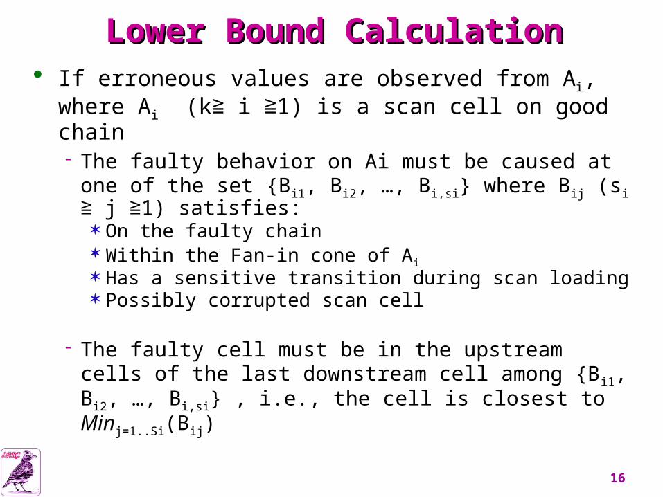
Lower Bound CalculationLower Bound Calculation If erroneous values are observed from Ai, where

Ai (k i 1) is a scan cell on good chain≧ ≧ The faulty behavior on Ai must be caused at one of

the set {Bi1, Bi2, …, Bi,si} where Bij (si j 1) ≧ ≧satisfies: On the faulty chain Within the Fan-in cone of Ai Has a sensitive transition during scan loading Possibly corrupted scan cell

The faulty cell must be in the upstream cells of the last downstream cell among {Bi1, Bi2, …, Bi,si} , i.e., the cell is closest to Minj=1..Si(Bij)

17

Lower Bound CalculationLower Bound Calculation

Lower_Bound ≧ Maxi=1..k(Minj=1..Si(Bij))

18

Calculate Lower Bound Calculate Lower Bound For Multiple Faulty ChainFor Multiple Faulty Chain

Step 1: If Minij upper bound≧ for the faulty chain j, use “—” to replaceMinij

Step 2: If Ai has only one item that is not “—”, chain j must be responsible for the observed fault at A i. If the lower bound is less than Minij, update the lower bound to Minij

Step 3: Apply more patterns to add more columns to the dependency table and repeat step1~2 until no more update for a specified no. of patterns

A1 A2 …… Ak

Lower Bound

Faulty Chain 1 Min11 Min21 …… Mink1 0

Faulty Chain 2 Min12 Min22 …… Mink2 0

…… …… …… …… …… 0

Faulty Chain n Min1n Min2n …… Minkn 0

19

Statistical DiagnosisStatistical Diagnosis Ranking: Calculate the probability of each candidate

faulty scan cell

Bayes theorem:

[X1, X2, …, Xn] is a partition of a set of all possible n outcomes of an event X

∵ P(xk) = 1/Length(j)

n

kkk

kkk

XYPXP

XYPXPYXP

1

)|()(

)|()()|(

n

kk

kk

XYP

XYPYXP

1

)|(

)|()|(

20

AssumptionAssumption UPj and LOj are the upper bound and lower

bound for the fault site on one scan chain j: If k is out of range [UPj , LOj ], P(Y|Xk)=0

Scan_in Scan_out

UPj LOj

0X10XX100

21

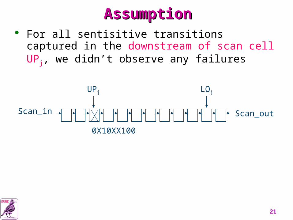
AssumptionAssumption For all sentisitive transitions captured in the

downstream of scan cell UPj, we didn’t observe any failures

Scan_in Scan_out

UPj LOj

0X10XX100

22

AssumptionAssumption When any sensitive transition loaded into [UPj ,

LOj ], we deterministically know whether this transition is possibly or impossibly to be corrupted

23

An Example for Statistical DiagnosisAn Example for Statistical Diagnosis

P1(Y|Xk) = (1-Prob)u if k U_Section[u] = 0 otherwise

P2(Y|Xk) = Prob *(1-Prob)l if k L_Section[l] = 0 otherwise

Prob = fault observed / total sensitive transition

P(Y|Xk) = P1(Y|Xk) * P2(Y|Xk)

24

Information of The Test CasesInformation of The Test Cases

Designs# of

simulated gates

# of PIs

# of POs

# of scan

chains

Lengths of the longest scan chain

# of faulty chains

Real faulty sites

F1 147000 95 86 8 725 2

Faulty Chain I: (301, 407)

Faulty chain II: (57)

F2 325996 64 51 10 897 1 10

M1 2679502 354 343 64 3184 —

25

Experimental ResultsExperimental Results

Designs # of applied scan patterns Upper bound Lower bound

The cells with the highest probability

F1 3

Faulty Chain I: 301

Faulty Chain I: 177

(299, 300, 301)

Faulty Chain II: 57

Faulty Chain II: 0 (57)

F2 16 13 8 (10, 11, 12, 13)

Diagnosis resolution = (# of candidate faulty cell with highest probability)-1

26

Experimental ResultsExperimental ResultsInjected faulty site # of patterns for diagnosis Probability of triggering fault Diagnosis resolution

Site 1

1060% 1880% 13

100% 11

2060% 780% 4

100% 4

3060% 780% 4

100% 4

Site 2

1060% 22

80% 17

100% 17

2060% 880% 5

100% 4

3060% 780% 3

100% 1

Site 3

1060% 1580% 15

100% 12

2060% 680% 6

100% 4

3060% 280% 1

100% 1

27

ConclusionConclusion Proposed a method to calculate an upper/lower

bound on the candidate faulty cells

The root causes of intermittent scan chain hold time faults are very difficult to model

Diagnosis of this problem is helpful to reduce cost of silicon debug and improve yield

This method is efficient and effective for large industrial design s with multiple faulty scan chains