STATISTICAL DESIGN AND ANALYSIS OF DAIRY NUTRITION ...
14
Kansas State University Libraries Kansas State University Libraries New Prairie Press New Prairie Press Conference on Applied Statistics in Agriculture 1989 - 1st Annual Conference Proceedings STATISTICAL DESIGN AND ANALYSIS OF DAIRY NUTRITION STATISTICAL DESIGN AND ANALYSIS OF DAIRY NUTRITION EXPERIMENTS TO IMPROVE DETECTION OF MILK RESPONSE EXPERIMENTS TO IMPROVE DETECTION OF MILK RESPONSE DIFFERENCES DIFFERENCES Stephen R. Lowry Follow this and additional works at: https://newprairiepress.org/agstatconference Part of the Agriculture Commons, and the Applied Statistics Commons This work is licensed under a Creative Commons Attribution-Noncommercial-No Derivative Works 4.0 License. Recommended Citation Recommended Citation Lowry, Stephen R. (1989). "STATISTICAL DESIGN AND ANALYSIS OF DAIRY NUTRITION EXPERIMENTS TO IMPROVE DETECTION OF MILK RESPONSE DIFFERENCES," Conference on Applied Statistics in Agriculture. https://doi.org/10.4148/2475-7772.1452 This is brought to you for free and open access by the Conferences at New Prairie Press. It has been accepted for inclusion in Conference on Applied Statistics in Agriculture by an authorized administrator of New Prairie Press. For more information, please contact [email protected].
Transcript of STATISTICAL DESIGN AND ANALYSIS OF DAIRY NUTRITION ...

Kansas State University Libraries Kansas State University Libraries
New Prairie Press New Prairie Press
Conference on Applied Statistics in Agriculture 1989 - 1st Annual Conference Proceedings
STATISTICAL DESIGN AND ANALYSIS OF DAIRY NUTRITION STATISTICAL DESIGN AND ANALYSIS OF DAIRY NUTRITION
EXPERIMENTS TO IMPROVE DETECTION OF MILK RESPONSE EXPERIMENTS TO IMPROVE DETECTION OF MILK RESPONSE
DIFFERENCES DIFFERENCES
Stephen R. Lowry
Follow this and additional works at: https://newprairiepress.org/agstatconference
Part of the Agriculture Commons, and the Applied Statistics Commons
This work is licensed under a Creative Commons Attribution-Noncommercial-No Derivative Works 4.0 License.
Recommended Citation Recommended Citation Lowry, Stephen R. (1989). "STATISTICAL DESIGN AND ANALYSIS OF DAIRY NUTRITION EXPERIMENTS TO IMPROVE DETECTION OF MILK RESPONSE DIFFERENCES," Conference on Applied Statistics in Agriculture. https://doi.org/10.4148/2475-7772.1452
This is brought to you for free and open access by the Conferences at New Prairie Press. It has been accepted for inclusion in Conference on Applied Statistics in Agriculture by an authorized administrator of New Prairie Press. For more information, please contact [email protected].

STATISTICAL DESIGN AND ANALYSIS OF DAIRY NUTRITION EXPERIMENTS TO IMPROVE DETECTION OF MILK RESPONSE DIFFERENCES
Stephen R. Lowry University of Kentucky
ABSTRACT
The objective of many dairy nutrition experiments is to determine the effect of certain dietary treatments on milk production and quality responses. However, milk responses are quite variable and cows (experimental units) are expensive and have substantial maintenance costs. This manuscript reviews principles for planning to obtain good data relevant to the hypothesis, experimental design to control inherent variation, and interpreted analyses to facilitate understanding of dairy relationships. Emphasis is placed :on assurance that milk response differences due to dietary treatments will have a high probability of being detected as significant. Guidelines addressing these principles along with suggested computer programs are presented. Results of two dairy nutrition experiments are included to illustrate use of the presented guidelines to maxlmlZe detection of real differences in milk response due to dietary treatments.
Key Words: Experimental Design, Dairy
1. INTRODUCTION
Most dairy nutrition experiments measure the effects of certain treatments (usually dietary) on milk production and quality. Those effects refer to response changes or differences due to treatments which have been measured empirically and then analyzed and interpreted using statistical procedures. An investigation should be planned to address specific questions or problems. The associated experiment, employing the scientific method, should be designed and executed so that analysis of the resulting data adequately addresses those questions and problems in hypothesis form.
Most dairy responses exhibit coefficients of variation from 8 to 25%. Gill (7) provides an excellent discussion complete with easily used graphs to quickly determine numbers of cows per treatment necessary to detect certain size differences with 50% or 80% prediction or examples. One notes that 10 cows per treatment are required to have a 50% chance of detecting a difference of 4.25 kilograms of daily milk yield (assuming average daily milk of 21 kg) with a coefficient of variance of 22.5% when a completely randomized experimental design is used. Gill also illustrates that modest reductions in cows required per treatment occur when a covariate of milk yield during first month of lactation or cows are blocked into milk yield groups. Substantial reductions in required number of cows occur when the crossover design is used. High purchase costs and maintenance costs during lactation make this level of precision difficult to attain. Thus, this manuscript reviews and documents experimental procedures whereby treatment differences in milk response have a high probability of being detected analytically with available animals and current time and labor constraints.
59
Conference on Applied Statistics in AgricultureKansas State University
New Prairie Presshttps://newprairiepress.org/agstatconference/1989/proceedings/7

60
2. iJiATERIALS Acl\jD METHODS
Experimental Procedures
Three major experimental components will improve the experimenter's ability to achieve the desired power for detecting treatment differences with a minimum of critical resources:
(1) careful planning; (2) selecting or developing appropriate experimental designs; (3) collecting, analyzing and interpreting research results.
Planning the Experiment
Planning should include a documented set of experimental procedures from initial stage to publishing the results (12). lL'1 exper~Tflent must be planned with cows and treatments so that the subsequent results address a specific relationship, expressed as a hypothesis (5, 10, 12, 22). The treatment effects may be explained further with regression or response surface analyses, orthogonal polynomials, planned contrast comparisons, or multiple mean comparisons. Draper, and Smith (4), Mead and Pike (14) and Snedecor and Cochran (21) provide excellent discussion and examples. Carmer and Walker (1) state that choice of significance level should be determined based on an assessment of the risks of both wrongly rejecting and wrongly accepting the null hypothesis. They suggest using weighted average risk. l~ experimental design should be chosen which removes extraneous variation and provides an appropriate test for the hypothesis (2, 5, 10, 21, 22). The availability and selection of experimental units must also be addressed. Sufficient resources and labor also must be available. Statistical consulting and research computing support may be needed to comprete appropriate analyses of the results especially with realistic but unwieldy problems such as the carryover of a treatment effect from one period to subsequent periods in a crossover design and repeated administration of a treatment which may i.ncrease or decrease milk response. Publication of interpreted results and conclusions is necessary to document an extended understanding of research relationships.
Experimental Design
General Experimental Techniques. The magnitude and causes of variability in milk responses must be recognized. Since more variable data require more animals and expense to attain equal precision, Federer (5) suggests refining experimental techniques to maximize power and quality of the data collection while minimizing cost. To apply this principle to milk response, plan and design the experiment to address, control or remove any known problem or source of variation, thereby reducing the experimental error (unexplained variation) and improving the probability of detecting real treatment differences. The error variance estimate also may be improved by carefully conducting the experiment, precisely measuring responses and arriving at a model which adequately represents the data (3, 8, 23).
Specific Desions for ~ Nutrition Experiments. Experimental design refers to this process of manipulating cow's condition and presentation of
Conference on Applied Statistics in AgricultureKansas State University
New Prairie Presshttps://newprairiepress.org/agstatconference/1989/proceedings/7

diets to cows in order to mlnlmlZe experimental error. A proper experiment should be replicated and randomized (6). Statistically, the estimate of experimental error, appropriate for testing for treatment differences, refers to variation of replicated experimental units. Biologically, replication allows the experimenter to study response consistency over all known sources of variation. A design for milk response data should classify individuals into similar subclasses and randomly allocate treatments to individuals within subclasses in order to obtain accurate estimates of treatment means and variances and nullify effects of uncontrolled variables. Lucas (14) has prepared a more comprehensive approach to design of good dairy experiments.
Applications of Widely Used Experimental Designs. Randomized complete block experiments will be sufficiently precise if the required number of animals is used (2). This design is appropriate for many current dairy nutrition full lactation experiments where treatments require longer terms for expression. When animals are limited, use of a covariate (continuous variable highly correlated with milk response but not affected by treatment) such as early short segment milk yields from 11 to 14 days may reduce required animal numbers by as much as 50% (11). If precision is still not sufficient, the experimenter may need to combine experiments over lactations and/or locations. McIntosh (16) provides an excellent summary of determining appropriate F ratios for combined experiments.
In trials where treatments are applied during the declining phase of cow lactation, when treatments express response in a period of a few weeks and when carryover of treatment effect is no more than one period, switchback designs and changeover (or crossover) designs are appropriate (3). The switchback design (11) controls variation by forcing each cow to be her own control thus achieving maximum precision with minimum resources. Each cow receives one treatment in period 1, a second treatment in period 2, and is switched back to the first treatment in period 3. The changeover design with two or more treatments (8, 9, 18) controls variation while examining treatment differences because each animal receives a random or balanced systematic sequence of all treatments in successive periods. Further, when treatment effects may carry over, the crossover design must be a balanced so residual effects can be separated from the direct treatment effects. Then, the statistical analysis separates the residuals from the direct treatment effects and compares direct treatment effects (3, 9). These designs generally lead to improved precision because variation within an~"als is less than between animals. The more general but related design, the latin square, removes two extraneous sources of variation from experimental error. While these two sources were cow and period for the previous designs, they may be herds, locations, years, managers, or other specific known sources of variation for the latin square. The only assumption required by the latin square in addition to those required by the randomized complete block is that no interaction may occur among rows, columns, and treatments and that number of treatments, rows, and columns are equal.
The randomized complete block, the latin square, and the changeover design without residual effects are easily analyzed using SAS programs. Heretofore, few dairy researchers have used switchbacks and changeovers with residual effects because analyses necessitated laborious hand calculations.
61
diets to cows in order to mlnlmlZe experimental error. A proper experiment should be replicated and randomized (6). Statistically, the estimate of experimental error, appropriate for testing for treatment differences, refers to variation of replicated experimental units. Biologically, replication allows the experimenter to study response consistency over all known sources of variation. A design for milk response data should classify individuals into similar subclasses and randomly allocate treatments to individuals within subclasses in order to obtain accurate estimates of treatment means and variances and nullify effects of uncontrolled variables. Lucas (14) has prepared a more comprehensive approach to design of good dairy experiments.
Applications of Widely Used Experimental Designs. Randomized complete block experiments will be sufficiently precise if the required number of animals is used (2). This design is appropriate for many current dairy nutrition full lactation experiments where treatments require longer terms for expression. When animals are limited, use of a covariate (continuous variable highly correlated with milk response but not affected by treatment) such as early short segment milk yields from 11 to 14 days may reduce required animal numbers by as much as 50% (11). If precision is still not sufficient, the experimenter may need to combine experiments over lactations and/or locations. McIntosh (16) provides an excellent summary of determining appropriate F ratios for combined experiments.
In trials where treatments are applied during the declining phase of cow lactation, when treatments express response in a period of a few weeks and when carryover of treatment effect is no more than one period, switchback designs and changeover (or crossover) designs are appropriate (3). The switchback design (11) controls variation by forcing each cow to be her own control thus achieving maximum precision with minimum resources. Each cow receives one treatment in period 1, a second treatment in period 2, and is switched back to the first treatment in period 3. The changeover design with two or more treatments (8, 9, 18) controls variation while examining treatment differences because each animal receives a random or balanced systematic sequence of all treatments in successive periods. Further, when treatment effects may carry over, the crossover design must be a balanced so residual effects can be separated from the direct treatment effects. Then, the statistical analysis separates the residuals from the direct treatment effects and compares direct treatment effects (3, 9). These designs generally lead to improved precision because variation within an~"als is less than between animals. The more general but related design, the latin square, removes two extraneous sources of variation from experimental error. While these two sources were cow and period for the previous designs, they may be herds, locations, years, managers, or other specific known sources of variation for the latin square. The only assumption required by the latin square in addition to those required by the randomized complete block is that no interaction may occur among rows, columns, and treatments and that number of treatments, rows, and columns are equal.
The randomized complete block, the latin square, and the changeover design without residual effects are easily analyzed using SAS programs. Heretofore, few dairy researchers have used switchbacks and changeovers with residual effects because analyses necessitated laborious hand calculations.
61 Conference on Applied Statistics in Agriculture
Kansas State University
New Prairie Presshttps://newprairiepress.org/agstatconference/1989/proceedings/7
62
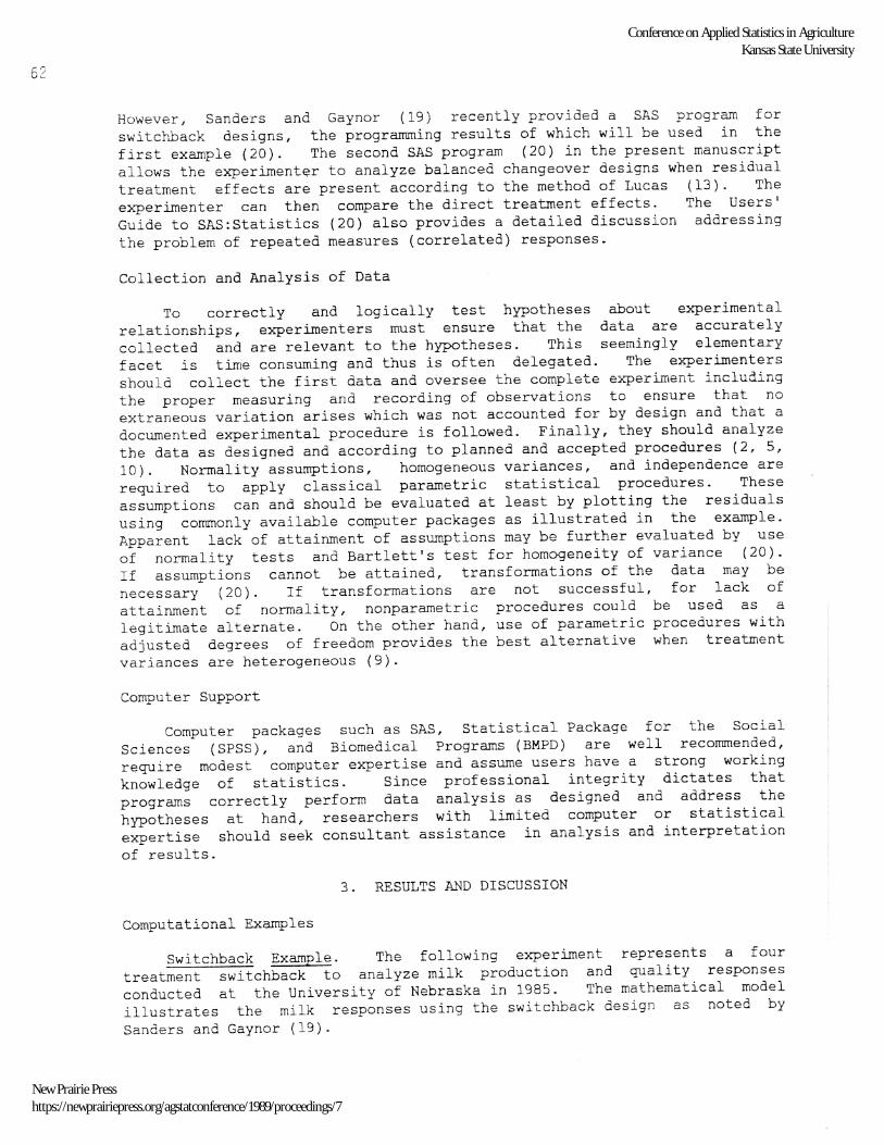
However, Sanders and Gaynor (19) recently provided a SAS program for switcr~ack designs, the programming results of which will be used in the first example (20). The second SAS program (20) in the present manuscript allows the experimenter to analyze balanced changeover designs when residual treatment effects are present according to the method of Lucas (l3). The experimenter can then compare the direct treatment effects. The Users' Guide to SAS:Statistics (20) also provides a detailed discussion addressing the problem of repeated measures (correlated) responses.
Collection and Analysis of Data
To correctly and logically test hypotheses about experimental relationships, experimenters must ensure that the data are accurately collected and are relevant to the hypotheses. This seemingly elementary facet is time consuming and thus is often delegated. The experimenters should collect the first data and oversee the complete experiment including the proper measuring and recording of observations to ensure that no extraneous variation arises which was not accounted for by design and that a documented experimental procedure is followed. Finally, they should analyze the data as designed and according to planned and accepted procedures (2, 5, 10). Normality assumptions, homogeneous variances, and independence are required to apply classical parametric statistical procedures. These assumptions can and should be evaluated at least by plotting the residuals using commonly available computer packages as illustrated in the example. Apparent lack of attair~ent of assumptions may be further evaluated by use of normality tests and Bartlett's test for homogeneity of variance (20). If assumptions cannot be attained, transformations of the data may be necessary (20). If transformations are not successful, for lack of attainment of normality, nonparametric procedures could be used as a legitimate alternate. On the other hand, use of parametric procedures with adjusted degrees of freedom provides the best alternative when treatment variances are heterogeneous (9).
Computer Support
computer packages such as SAS, Statistical Package for the Social Sciences (SPSS), and Biomedical Programs (BMPD) are well recommended, require modest computer expertise and assume users have a strong working knowledge of statistics. Since professional integrity dictates that programs correctly perform data analysis as designed and address the hypotheses at hand, researchers with limited computer or statistical expertise should seek consultant assistance in analysis and interpretation of results.
3. RESULTS AND DISCUSSION
Computational Examples
Switchback Example. The following experiment represents a four treatment switchback to analyze milk production and quality responses conducted at the University of Nebraska in 1985. The mathematical model illustrates the milk responses using the switchback design as noted by Sanders and Gaynor (19).
62
However, Sanders and Gaynor (19) recently provided a SAS program for switcr~ack designs, the programming results of which will be used in the first example (20). The second SAS program (20) in the present manuscript allows the experimenter to analyze balanced changeover designs when residual treatment effects are present according to the method of Lucas (l3). The experimenter can then compare the direct treatment effects. The Users' Guide to SAS:Statistics (20) also provides a detailed discussion addressing the problem of repeated measures (correlated) responses.
Collection and Analysis of Data
To correctly and logically test hypotheses about experimental relationships, experimenters must ensure that the data are accurately collected and are relevant to the hypotheses. This seemingly elementary facet is time consuming and thus is often delegated. The experimenters should collect the first data and oversee the complete experiment including the proper measuring and recording of observations to ensure that no extraneous variation arises which was not accounted for by design and that a documented experimental procedure is followed. Finally, they should analyze the data as designed and according to planned and accepted procedures (2, 5, 10). Normality assumptions, homogeneous variances, and independence are required to apply classical parametric statistical procedures. These assumptions can and should be evaluated at least by plotting the residuals using commonly available computer packages as illustrated in the example. Apparent lack of attair~ent of assumptions may be further evaluated by use of normality tests and Bartlett's test for homogeneity of variance (20). If assumptions cannot be attained, transformations of the data may be necessary (20). If transformations are not successful, for lack of attainment of normality, nonparametric procedures could be used as a legitimate alternate. On the other hand, use of parametric procedures with adjusted degrees of freedom provides the best alternative when treatment variances are heterogeneous (9).
Computer Support
computer packages such as SAS, Statistical Package for the Social Sciences (SPSS), and Biomedical Programs (BMPD) are well recommended, require modest computer expertise and assume users have a strong working knowledge of statistics. Since professional integrity dictates that programs correctly perform data analysis as designed and address the hypotheses at hand, researchers with limited computer or statistical expertise should seek consultant assistance in analysis and interpretation of results.
3. RESULTS AND DISCUSSION
Computational Examples
Switchback Example. The following experiment represents a four treatment switchback to analyze milk production and quality responses conducted at the University of Nebraska in 1985. The mathematical model illustrates the milk responses using the switchback design as noted by Sanders and Gaynor (19).
Conference on Applied Statistics in AgricultureKansas State University
New Prairie Presshttps://newprairiepress.org/agstatconference/1989/proceedings/7

Yijk = u + cowi + biPj + Period j + Trtk + Eijk (1)
Yijk observed milk response of the i th cow in the j th period receiving the k th treatment,
u = overall mean
cow i = random effect of the i th individual cow
bi = regression coefficient of the response variable on period for the i th cow.
Pj = j th period (fixed continuous variable)
Period j = effect of the j th period (class variable which estimates the envirolli~ental effect throughout the study).
Trtk = fixed effect of the k th treatment
Eijk random error associated with ijk th observation [estimated from pooling of higher order interactions involving period, treatment and cow, which is consistent with error term components described by Lucas (13)J. Eijk is assumed to be normally distributed with zero expected mean and variance 0 2 Lucas (13) prepared this design based on the assumption that milk responses were linear after the peak of lactation. However, b Pj allows each cow to have a different persistency and different slope.
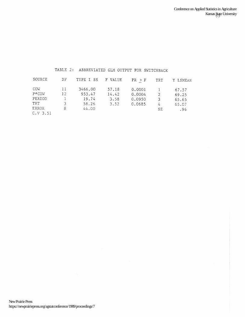
Table 1 contains a SAS program to analyze the results of this experiment. The statements produce the analysis of variance, treatment means, standard errors and plots of residuals from which to evaluate attainment of assumptions. The variables COW, p*COW, and PERIOD in the SAS program remove the same sources of variation from the cow-period means which are removed by calculating D = Yl -2 Y2 + Y3 (Yi = milk response in period i) for each cow in the original theoretically derived Lucas analysis (13). The equivalence is also justified by Sanders and Gaynor (19). The Fstatistic associated with the sequential (Type I) sums of squares is equivalent to that from using Lucas's original procedures (13). Table 2 displays an abbreviated PROC GLM listing. Sanders and Gaynor (19) developed a SAS mapping of the Lucas (13) analysis of the switchback design.
All procedures suggested herein were employed in this experiment. The experiment was carefully planned to address milk production response as affected by 4 treatments. Due to tight research budgets and because treatments were expected to express themselves within one month, the switchback eA~erimental design was successfully employed to obtain desired precision. Cows were randomly selected from a homogenous pool. The investigators closely monitored the experiment. Careful experimentation was successful in that the coefficient of variation was 3.51%. Thus, the experiment had high probability of detecting a real difference if one existed. The resulting F test was nonsignificant causing the experimenters to state that there was insufficient evidence to conclude the treatments were different at ~ = .05. These results duplicate the analysis of this experiment using Lucas's (13) original computational formulas.
Yijk = u + cowi + biPj + Period j + Trtk + Eijk (1)
Yijk observed milk response of the i th cow in the j th period receiving the k th treatment,
u = overall mean
cow i = random effect of the i th individual cow
bi = regression coefficient of the response variable on period for the i th cow.
Pj = j th period (fixed continuous variable)
Period j = effect of the j th period (class variable which estimates the envirolli~ental effect throughout the study).
Trtk = fixed effect of the k th treatment
Eijk random error associated with ijk th observation [estimated from pooling of higher order interactions involving period, treatment and cow, which is consistent with error term components described by Lucas (13)J. Eijk is assumed to be normally distributed with zero expected mean and variance 0 2 Lucas (13) prepared this design based on the assumption that milk responses were linear after the peak of lactation. However, b Pj allows each cow to have a different persistency and different slope.
Table 1 contains a SAS program to analyze the results of this experiment. The statements produce the analysis of variance, treatment means, standard errors and plots of residuals from which to evaluate attainment of assumptions. The variables COW, p*COW, and PERIOD in the SAS program remove the same sources of variation from the cow-period means which are removed by calculating D = Yl -2 Y2 + Y3 (Yi = milk response in period i) for each cow in the original theoretically derived Lucas analysis (13). The equivalence is also justified by Sanders and Gaynor (19). The Fstatistic associated with the sequential (Type I) sums of squares is equivalent to that from using Lucas's original procedures (13). Table 2 displays an abbreviated PROC GLM listing. Sanders and Gaynor (19) developed a SAS mapping of the Lucas (13) analysis of the switchback design.
All procedures suggested herein were employed in this experiment. The experiment was carefully planned to address milk production response as affected by 4 treatments. Due to tight research budgets and because treatments were expected to express themselves within one month, the switchback eA~erimental design was successfully employed to obtain desired precision. Cows were randomly selected from a homogenous pool. The investigators closely monitored the experiment. Careful experimentation was successful in that the coefficient of variation was 3.51%. Thus, the experiment had high probability of detecting a real difference if one existed. The resulting F test was nonsignificant causing the experimenters to state that there was insufficient evidence to conclude the treatments were different at ~ = .05. These results duplicate the analysis of this experiment using Lucas's (13) original computational formulas.
Conference on Applied Statistics in AgricultureKansas State University
New Prairie Presshttps://newprairiepress.org/agstatconference/1989/proceedings/7
64
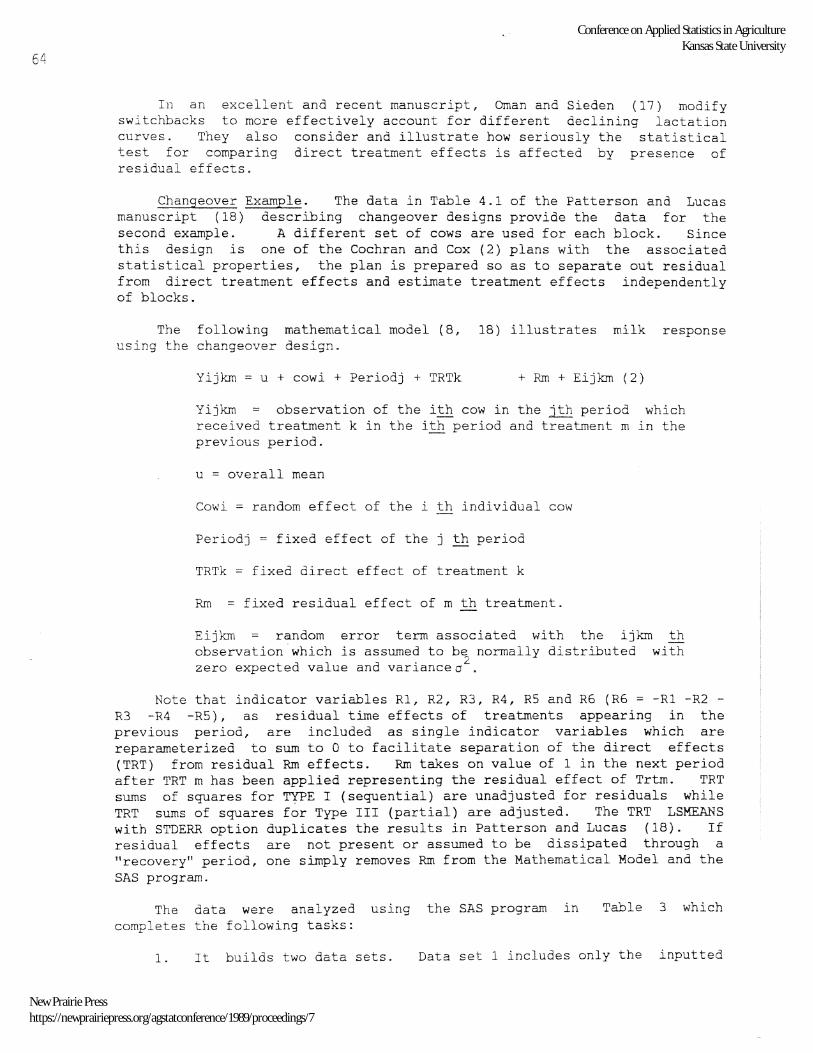
In an excellent and recent manuscript, Oman and Sieden (17) modify switchbacks to more effectively account for different declining lactation curves. They also consider and illustrate how seriously the statistical test for comparing direct treatment effects is affected by presence of residual effects.
Changeover Example. The data in Table 4.1 of the Patterson and Lucas manuscript (18) describing changeover designs provide the data for the second example. A different set of cows are used for each block. Since this design is one of the Cochran and Cox (2) plans with the associated statistical properties, the plan is prepared so as to separate out residual from direct treatment effects and estimate treatment effects independently of blocks.
The following mathematical model (S, IS) illustrates milk response using the changeover design.
Yijkm = u + cowi + Periodj + TRTk + Rm + Eijkm (2)
Yijkm observation of the ith cow in the jth period which received treatment k in the ith period and treatment m in the previous period.
u = overall mean
Cowi = random effect of the i th individual cow
Periodj = fixed effect of the j th period
TRTk = fixed direct effect of treatment k
Rm fixed residual effect of m th treatment.
Eijkm random error term associated with the ijkm th observation which is assumed to be normally distributed with zero expected value and variance 0 2 .
Note that indicator variables Rl, R2, R3, R4, R5 and R6 (R6 = -Rl -R2 -R3 -R4 -R5), as residual time effects of treatments appearing in the previous period, are included as single indicator variables which are reparameterized to sum to 0 to facilitate separation of the direct effects (TRT) from residual Rm effects. Rm takes on value of 1 in the next period after TRT m has been applied representing the residual effect of Trtm. TRT sums of squares for TYPE I (sequential) are unadjusted for residuals while TRT sums of squares for Type III (partial) are adjusted. The TRT LSMEANS with STDERR option duplicates the results in Patterson and Lucas (IS). If residual effects are not present or assumed to be dissipated through a "recovery" period, one simply removes Rm from the Mathematical Model and the SAS program.
The data were analyzed using the SAS program in completes the following tasks:
Table 3 which
1. It builds two data sets. Data set 1 includes only the inputted
64
In an excellent and recent manuscript, Oman and Sieden (17) modify switchbacks to more effectively account for different declining lactation curves. They also consider and illustrate how seriously the statistical test for comparing direct treatment effects is affected by presence of residual effects.
Changeover Example. The data in Table 4.1 of the Patterson and Lucas manuscript (18) describing changeover designs provide the data for the second example. A different set of cows are used for each block. Since this design is one of the Cochran and Cox (2) plans with the associated statistical properties, the plan is prepared so as to separate out residual from direct treatment effects and estimate treatment effects independently of blocks.
The following mathematical model (S, IS) illustrates milk response using the changeover design.
Yijkm = u + cowi + Periodj + TRTk + Rm + Eijkm (2)
Yijkm observation of the ith cow in the jth period which received treatment k in the ith period and treatment m in the previous period.
u = overall mean
Cowi = random effect of the i th individual cow
Periodj = fixed effect of the j th period
TRTk = fixed direct effect of treatment k
Rm fixed residual effect of m th treatment.
Eijkm random error term associated with the ijkm th observation which is assumed to be normally distributed with zero expected value and variance 0 2 .
Note that indicator variables Rl, R2, R3, R4, R5 and R6 (R6 = -Rl -R2 -R3 -R4 -R5), as residual time effects of treatments appearing in the previous period, are included as single indicator variables which are reparameterized to sum to 0 to facilitate separation of the direct effects (TRT) from residual Rm effects. Rm takes on value of 1 in the next period after TRT m has been applied representing the residual effect of Trtm. TRT sums of squares for TYPE I (sequential) are unadjusted for residuals while TRT sums of squares for Type III (partial) are adjusted. The TRT LSMEANS with STDERR option duplicates the results in Patterson and Lucas (IS). If residual effects are not present or assumed to be dissipated through a "recovery" period, one simply removes Rm from the Mathematical Model and the SAS program.
The data were analyzed using the SAS program in completes the following tasks:
Table 3 which
1. It builds two data sets. Data set 1 includes only the inputted
Conference on Applied Statistics in AgricultureKansas State University
New Prairie Presshttps://newprairiepress.org/agstatconference/1989/proceedings/7

data. Data set 2 includes only cow, period, clock and a created residual treatment code.
2. Period, cow, block, treatment and milk response are defined and formatted in an input statement.
3. Assignment statements are used for number of periods and nurober of treatments and are named LASTPER and LASTTRT, respectively_ Thus, the program could be easily altered for different number of periods and treatments.
4. A value of 0 is given for TRTRES as residual treatment for period 1 since no residual effect is present.
5. When period is greater than 1 but less than the last period, TRTRES in the next period is given the TRT val~e for the current period using an indicator function.
6. The raw data are then read in.
7. The two data sets are sorted and merged to build a complete data set including original data and created TRTRES.
8. An array is built for creating single columns of residual treatment effects for each treatment. The residuals were created from an indicator function using a SAS function which takes a value of 1 when the statement within parenthesis is true and 0 otherwise. Then, the model as stated by Gill and Magee (8) was placed in SAS augmented by single columns of the residual treatment effects so the direct treatment effects adjusted for the residual effects could be estimated, which are equivalent to those computed by Patterson and Lucas (18).
The appropriate F test for comparing adjusted treatments means is derived from the TYPE III (partial) SQ~S of squares because these direct treatment effects are adjusted for residual treatment effects. Note that the sum of the sums of squares for Rl - R5 for Type I sum of squares is 3.8843 which is equivalent to the computed value in Patterson and Lucas (18). Table 4 displays an abbreviated ANOVA and PROL GLM listing.
The experLmenter is cautioned to address cyclic variation in feed intake data (if included as a response) that can cause upward bias in error mean squares in row-column designs. stroup et a1. (24) suggest corrective measures for this problem.
In subse~Jent experiments, one should attempt to determine any measureab1e continuous characteristics of cows and experimental conditions, the variation of which could be removed from the estimate of experimental error using ~ovariance analysis or blocking. Further, the experimenter should make notes of any difficulties in current experiments which could be addressed in the planning and design stage of new investigations.
65
data. Data set 2 includes only cow, period, clock and a created residual treatment code.
2. Period, cow, block, treatment and milk response are defined and formatted in an input statement.
3. Assignment statements are used for number of periods and nurober of treatments and are named LASTPER and LASTTRT, respectively_ Thus, the program could be easily altered for different number of periods and treatments.
4. A value of 0 is given for TRTRES as residual treatment for period 1 since no residual effect is present.
5. When period is greater than 1 but less than the last period, TRTRES in the next period is given the TRT val~e for the current period using an indicator function.
6. The raw data are then read in.
7. The two data sets are sorted and merged to build a complete data set including original data and created TRTRES.
8. An array is built for creating single columns of residual treatment effects for each treatment. The residuals were created from an indicator function using a SAS function which takes a value of 1 when the statement within parenthesis is true and 0 otherwise. Then, the model as stated by Gill and Magee (8) was placed in SAS augmented by single columns of the residual treatment effects so the direct treatment effects adjusted for the residual effects could be estimated, which are equivalent to those computed by Patterson and Lucas (18).
The appropriate F test for comparing adjusted treatments means is derived from the TYPE III (partial) SQ~S of squares because these direct treatment effects are adjusted for residual treatment effects. Note that the sum of the sums of squares for Rl - R5 for Type I sum of squares is 3.8843 which is equivalent to the computed value in Patterson and Lucas (18). Table 4 displays an abbreviated ANOVA and PROL GLM listing.
The experLmenter is cautioned to address cyclic variation in feed intake data (if included as a response) that can cause upward bias in error mean squares in row-column designs. stroup et a1. (24) suggest corrective measures for this problem.
In subse~Jent experiments, one should attempt to determine any measureab1e continuous characteristics of cows and experimental conditions, the variation of which could be removed from the estimate of experimental error using ~ovariance analysis or blocking. Further, the experimenter should make notes of any difficulties in current experiments which could be addressed in the planning and design stage of new investigations.
65 Conference on Applied Statistics in Agriculture
Kansas State University
New Prairie Presshttps://newprairiepress.org/agstatconference/1989/proceedings/7

66
4. SUMMARY
This manuscript reviews and documents experimental procedures whereby treatment differences in highly variable milk responses have a high probability 9f being ,detected analytically. More sophisticated experimental designs are suggested: and illustrated which maximize power and data quality while minimizing cost. Two examples are employed to illustrate discussed principles.
SAS is Mention of endorsement
ACKNOWLEDGMENTS
the registered trademark of SAS Institute, the name of a proprietary product is not
of the product as superior to others which
Inc., Cary, N. C. to be considered an may also be suitable.
Appreciation is expressed to F. G. Owen and A. O. Edionwe the first example data. Appreciation is also expressed to P. for providing ideas and assistance with SAS programs.
for providing L. Cornelius
1.
2.
Carmer, S. G. and W. statistician's viewpoint.
REFERENCES
M. Walker. 1988. J. Prod. Agric. 1:27.
Significance from a
Cochran, Edition.
W. G. and G. M. Cox. 1957. Experimental designs. Second John Wiley and Sons, New York, NY.
3. Damon, R. A. and Harvey, W. R. 1987. regression. Harper and Row, New York, NY.
Experimental design, anova,
4. D~aper, N. R. and H. Smith. 1966. Applied regression analysis. John Wiley and Sons, New York, NY.
5. Federer, W. T. 1955. Experimental design theory and application. MacMillan, New York, NY.
6. Fisher, R. A. 1949. The design of experiments. Fifth Edition. Oliver and Boyd, London.
7. Gill, J. L. 1969. Sample size for experiments on milk yield. J. Dairy Sci. 52: 984.
8. Gill, J. L. and W. T. Magee. 1976. Balanced two-period changeover designs for several treatments. J. Anim. Sci. 42:775.
9. Gill, J. L. 1978. Design and analysis of experiments in the animal and medical sciences. Vol. 2, Iowa State University Press, Ames, IA.
10. Hicks, C. R. 1973. Fundamental concepts in the design of experiments. Second Edition. Holt, Rinehart and Winston, Chicago, IL.
11. Lowry, S. R. and F. G. Owen. 1981. Potential of milk yield in short segments of early lactation as covariates in feeding experiments. J. Dairy Sci. 3:533.
Conference on Applied Statistics in AgricultureKansas State University
New Prairie Presshttps://newprairiepress.org/agstatconference/1989/proceedings/7

12. Lowry, S. R. 1979. Statistical planning and designing of experiments to detect differences in sensory evaluation of beef loin steaks. J. Food Sci. 44:488.
13. Lucas, H. L. 1956. Switchback trials for more than two treatments. J.
14.
Dairy Sci. 39:146.
Lucas, H. experiments.
L. 1960. Critical features of good dairy feeding J. Dairy Sci. 43:193.
15. Mead, R. and D. J. Pike. 1975. A review of response surface methodology from a biometric viewpoint. Biometrics. 31:803.
16. Hclntosh, 11. S. 1983. Analysis of combined experiments. Agronomy J. 75:153.
17. Oman, S. D. and D. Seiden. 1988. 75:81.
Switchback designs. Biometrika.
18. Patterson, Bull. No. Agric.
H. D. and H. L. Lucas. 1962. Changeover designs. Technical 147. North Carolina Agric. Exp. sta. and U. S. Department
19. Sanders, W. L. and P. J. Gaynor. 1987. Analysis of switchback data using Statistical Analysis System Inc. software. J. Dairy Sci. 70:2186.
20. SAS Institute, Inc. 1985. SAS User's Guide: statistics. Version 5. Cary, N.C.
21. Snedecor, G. W. and W. G. Cochran. 1980. Statistical methods. Seventh Edition. Iowa State University Press, Ames, IA.
22. Steel, R. G. D. and J. H. Torrie. 1980. Principles and procedures in statistics. Second Edition. McGraw-Hill, New York, NY.
23. Stock, R. A., T. J. Klopfenstein, D. R. Brink, S. R. Lowry, D. Rock, and S. Abrams. 1983. Impact of weighing procedures and variation in protein degradation rate in measured performance on growing lambs and cattle. J. Anim. Sci. 57:1276.
24. Stroup, W. W., M. K. Nielsen, and J. A. Gosey. 1987. in cattle feed intake data: characterization and experimental design. J. ~~irn. Sci. 64:1638.
Cyclic variation implications for
67
Conference on Applied Statistics in AgricultureKansas State University
New Prairie Presshttps://newprairiepress.org/agstatconference/1989/proceedings/7

68
TABLE 1: PROGRAMMING STATEMENTS TO ANALYZE A CROSSOVER EXPERIMENT;
DATA DSl(DROP:TRTRES) DS2(KEEP:COW PER BLK TRTRES); ~COMMENT DS1 INCLUDES ONLY INPUTTED DATA; *COMMENT DS2 INCLUDES CLASSIFICATION VARIABLES AND CREATED RESIDUAL CODE; INPUT PER 1 COW 3 BLK 5 TRT 7 FCM 26-30; *COMMENT FORMAT FOR INPUT VARIABLES IS INCLUDED HERE; LASTPER:4;LASTTRT:6;OUTPUT DSl; ~COMMENT DESIGNATION OF NUMBER OF TREATMENTS AND PERIODS; IF PER:l THEN DO; TRTRES:O; OUTPUT DS2; END; *COMMENT DEFINE INITIAL VALUE FOR RESIDUAL TRT; IF PER LT LASTPER THEN DO; PER:PER +1; TRTRES:TRT; OUTPUT DS2; END; *COMMENT TRTRES IN THE NEXT PERIOD IS GIVEN TRT VALUE IN CURRENT PERIOD; *COMMENT INPUT DATA HERE;
138.7 137.4
CARDS; 1111100000 2 1 1 4 I 1 0 0 0 0 311210001 411510100 121210000
o 134.3
2 2 1 1 I 0 1 0 0 3 2 1 5 I 1 0 0 0 421410000 131510000 2 3 1 2 I 0 000
o 131.3 o 148.9 o 146.9 o 142.0 1 139.6 o 134.6 1 132.3 o 128.5
127.1 135.2 133.5 128.4 125.1 132.9 133.1 127.5 125.1 130.4 129.5 126.7 123.1 130.8 129.3 126.4 123.2 125.7 126.1 123.4 118.7 125.4 126.0 123.9 119.9 121. 8 123.9 121. 7 117.6 121. 4 122.0 119.4 116.6 122.8 121. 0 118.6
3 3 1 4 I 0 100 4311100010 1 4 1 4 I 0 0 0 0 0 2 4 1 5 I 0 0 0 1 0 3 4 1 1 I 0 0 0 0 1 4 4 1 2 I 1 0 0 0 0 1 124 I 0 0 0 0 0 2121100010 31261 1 0 0 0 0 4 1 2 3 1-1 -1 -1 -1 -1 122 6 I 0 0 0 0 0 2 2 2 1-1 -1 -1 -1 -1 3 2 2 3 I 0 0 0 1 0 4221100100 1 3 2 3 I 0 0 0 0 0 23261 0 0 1 0 0 3 3 2 1 1-1 -1 -1 -1 -1 4 324 I 1 0 0 0 0 1 421 I 0 0 0 0 0 2 4 2 3 I 1 0 0 0 0 3 4 2 4 I 0 0 1 0 0 4426100010 1135100000 2 1 3 ~ I 0 0 b 0 1 3 1 3 2 1-1 -1 -1 -1 -1 4133101000 1232100000 2 2 3 5 I 0 1 0 0 0 3233100001 4 2 3 6 I 0 0 1 0 0 1336100000 2 3 3 3 1-1 -1 -1 -1 -1 3335100100 4332100001 1433100000 2432100100 3436101000
4 3 5 1-1 -1 -1 -1 -1 PROC SORT DATA:DS2; BY PROC PRINT;
116 .1 BLK COW PER;
PROC SORT DATA:DSl; BY BLK COW PER; PROC PRINT; DATA DS3; MERGE DSI DS2; BY BLK COW PER; *COMMENT DATA ARE SORTED AND MERGED TO CREATE ONE COMPLETE DATA SET; ARRAY R(I) RI-R5; DO 1:1 TO 5; R:(TRTRES:I) - (TRTRES:LASTTRT);END; *CO~MENT SINGLE COLUMNS OF RESIDUAL TREATMENT EFFECTS ARE CREATED; *COMMENT THE COLUt1NS OF CREATED RESIDUAL EFFECTS ARE PLACED BETWEEN I SYMBOLS AS THEY WOULD APPEAR IN THE DATA SET IF READ IN;
Conference on Applied Statistics in AgricultureKansas State University
New Prairie Presshttps://newprairiepress.org/agstatconference/1989/proceedings/7
69
TABLE 2: ABBREVIATED GL~ OUTPUT FOR SWITCHBACK
SOURCE DF TYPE I S8 F VALUE PR > F TRT Y L8MEAN -
COW 11 3466.00 57.18 0.0001 1 67.57 P*COW 12 953.47 14.42 0.0004 2 69.25 PERIOD 1 19.74 3.58 0.0950 3 65.65 TRT 3 58.26 3.52 0.0685 /, 65.07 "" ERROR 8 44.00 SE .96 C.V 3.51
69
TABLE 2: ABBREVIATED GL~ OUTPUT FOR SWITCHBACK
SOURCE DF TYPE I S8 F VALUE PR > F TRT Y L8MEAN -
COW 11 3466.00 57.18 0.0001 1 67.57 P*COW 12 953.47 14.42 0.0004 2 69.25 PERIOD 1 19.74 3.58 0.0950 3 65.65 TRT 3 58.26 3.52 0.0685 /, 65.07 "" ERROR 8 44.00 SE .96 C.V 3.51
Conference on Applied Statistics in AgricultureKansas State University
New Prairie Presshttps://newprairiepress.org/agstatconference/1989/proceedings/7

70
TABLE 3: PROGRAMMING STATEMENTS TO ANALYZE A SWITHCHBACK
DATA SWTCHBCK; INPUT TRT PERIOD COW Y; P=PERIOD; * COMMENT- INPUT DATA HERE; CARDS; 1 1 3336 70.8 2 2 3336 65.5 1 3 3336 60.1 1 1 3300 96.2 4 2 3300 85.1 1 3 3300 82.3 1 1 636 74.7 3 2 636 72.3 1 3 636 65.8 2 1 3415 75.5 4 2 3415 68.5 2 3 3415 66.3 2 1 3259 69.1 3 2 3259 62.6 2 3 3259 57.7 2 1 603 76.7 1 2 603 70.5 2 3 603 69.0 3 1 3497 78.4 1 2 3497 7l. 9 3 3 3497 62.0 3 1 3175 58.5 2 2 3175 63.8 3 3 3175 50.4 3 1 617 64.4 4 2 617 66.1 3 3 617 60.4 4 1 3476 77.7 3 2 3476 79.1 4 3 3476 73.3 4 1 3428 61. 9 1 2 3428 53.3 4 3 3428 36.5 4 1 632 60.1 2 2 632 56.5 4 3 632 44.9 PROC PRINT; PROC GLM; CLASSES COW TRT PERIOD MODEL Y =COW p*COW PERIOD TRT; LSMEANS TRT/S P; ESTIMATE 'TRT 1 - TRT 2' TRT 1 -1 0 0; ESTIMATE 'TRT 1 - TRT 3' TRT 1 0 -1 0; ESTIMATE 'TRT 1 - TRT 4' TRT 1 0 0 -1; ESTIMATE 'TRT 2 - TRT 3' TRT 0 1 -1 0; ESTIMATE 'TRT 2 - TRT 4' TRT 0 1 0 -1; ESTIMATE 'TRT 3 - TRT 4' TRT 0 0 1 -1; OUTPUT OUT=NEW PREDICTED=PREDY RESIDUAL=RESIDY; PROC PLOT; PLOT PREDY*RESIDY;
EXPERIMENT;
*COMMENT- THE LAST TWO LINES REPRESENT A PLOT OF THE RESIDUALS. THE PLOTS SHOULD BE IN AN ELLIPTICAL FORM WITH VERTICAL AND HORIZONTAL AXES. ANY DEVIATION INDICATES THAT ASSUMPTIONS MAY NOT BE ATTAINED; *COMMENT- SAS PROGRAMMING STATEMENTS TO ANALYZE SWITCHBACK DATA;
Conference on Applied Statistics in AgricultureKansas State University
New Prairie Presshttps://newprairiepress.org/agstatconference/1989/proceedings/7

71
TABLE 4: ABBREVIATED GLM OUTPUT FOR CHANGEOVER
SOURCE DF TYPE I SS SOURCE TYPE III SS
PER 3 388.30 PER 388.30 BLK 2 1607.01 BLK 838.68 PER*BLK 6 19.74 PER*BLK 19.48 cow (BLK) 9 628.71 COW (BLK) 611. 20 TRT (Unadjusted) 5 2.50 TRT (Adjusted) 3.14 R1 1 0.27 R1 1.02 R2 1 0.18 R2 0.08 R3 1 0.31 R3 0.00 R4 1 3.12 R4 2.90 R5 1 0.00 R5 0.00 Error 17 9.32
FCM STDERR F Value PR > F TRT LSMEAN LSMEAN
TRT (Unadjusted) .91 .4964 1 27.7629 0.287 TRT (Adj usted) 1.15 .3750 2 27.5431 0.287 C.V 2.66 3 28.1015 0.287
4 28.0954 0.287 5 27.8669 0.287 6 27.3552 0.287
Conference on Applied Statistics in AgricultureKansas State University
New Prairie Presshttps://newprairiepress.org/agstatconference/1989/proceedings/7