C OORDINATING SERVICES FOR ACCESSING AND PROCESSING DATA IN DYNAMIC ENVIRONMENTS .
date post
20-Dec-2015Category
view
218download
3
Statistical, Computational, and Informatics Tools for Biomarker
Analysis
Methodology Development at the
Data Management and Coordinating Center
of the
Early Detection Research Network
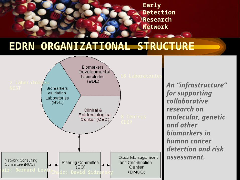
18 Laboratories
8 CentersCDCP
2 LaboratoriesNIST
Chair: David SidranskyChair: Bernard Levin
EDRN ORGANIZATIONAL STRUCTURE
An “infrastructure” for supporting collaborative research on molecular, genetic and other biomarkers in human cancer detection and risk assessment.
EarlyDetectionResearch Network
• Specimens with matching controls and epidemiological data• Infrastructure to provide preneoplastic tissues: - Prostate
- Lung- Ovarian- Colon- Breast
BIOREPOSITORY
EarlyDetectionResearch Network
INFRASTRUCTURE
EarlyDetectionResearch Network
INFRASTRUCTURE
• Capability in high-throughput molecular and biochemical assays
• Ability to respond to evolving technologies for EDRN needs
• Extensive experience and scale-up ability in proteomics and molecular assays
• Outstanding infrastructure for handling multiple assays and validation requests
LABORATORY CAPACITY
EarlyDetectionResearch Network
INFRASTRUCTURE
• Outstanding track record in biomarker research
• Statistical and data mining technology
• Statistical and predictive models for multiple biomarkers
• Novel statistical methods to interpret high-throughput data
DATA STORAGE AND MINING
EarlyDetectionResearch Network
INFRASTRUCTURE
•Improving informatics and information flow
Network web sites public web sitesecure web site
• Early Detection Research Network Exchange (ERNE)
• Standardizing of Data Reporting: CDEs Developed
DATA EXCHANGE AND SHARING
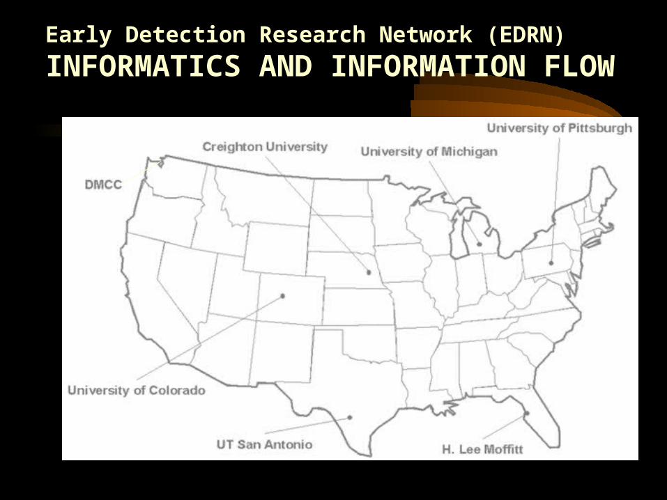
Early Detection Research Network (EDRN)
INFORMATICS AND INFORMATION FLOW
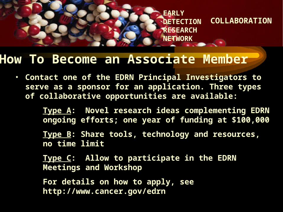
• Contact one of the EDRN Principal Investigators to serve as a sponsor for an application. Three types of collaborative opportunities are available:
Type A: Novel research ideas complementing EDRN ongoing efforts; one year of funding at $100,000
Type B: Share tools, technology and resources, no time limit
Type C: Allow to participate in the EDRN Meetings and Workshop
For details on how to apply, see http://www.cancer.gov/edrn
How To Become an Associate Member
EARLYDETECTIONRESEARCHNETWORK
COLLABORATION
DMCC Statisticians
• Margaret Pepe, Lead of Methodology Group
• Ziding Feng, Principal Investigator
• Yinsheng Qu
• Mary Lou Thompson
• Mark Thornquist
• Yutaka Yasui

Biomarker Lab Collaborators at Eastern Virginia Medical School
• Bao-Ling Adam
• John Semmes
• George Wright

Focus of Presentation
• Design:Phase Structure for Biomarker Research
• Analysis:Statistical Methods for Biomarker Discovery from High-Dimensional Data Sets
Design: Phase Structure for Biomarker Research
Three phase structure for therapeutic trials well-established
Structure promotes coherent, thorough, efficient development
Similar structure needs to be developed for biomarker research
Biomarker Development
• Categorize process into 5 phases
• Define objectives for each phase
• Define ideal study designs, evaluation and criteria for proceeding further
• Standardize the process to promote efficiency and rigor

Figure 2. Phases of Biomarker Development
Preclinical Exploratory
PHASE 1 Promising directions identified
Clinical Assay and Validation
PHASE 2 Clinical assay detects established disease
Retrospective Longitudinal PHASE 3
Biomarker detects preclinical disease and a “screen positive” rule defined
Prospective Screening
PHASE 4 Extent and characteristics of disease detected by the test and the false referral rate are identified
Cancer Control PHASE 5
Impact of screening on reducing burden of disease on population is quantified
The Details of Study Design
• Specific Aims
• Subject/Specimen Selection
• Outcome measures
• Evaluation of Results
• Sample Size Calculations
• Limitations / Pitfalls

Specific Aims
Phase 1• Identify leads for
potentially useful biomarkers
• Prioritize these leads
Phase 2• Determine the
sensitivity and specificity or ROC curve for the clinical biomarker assay in discriminating clinical cancer from controls
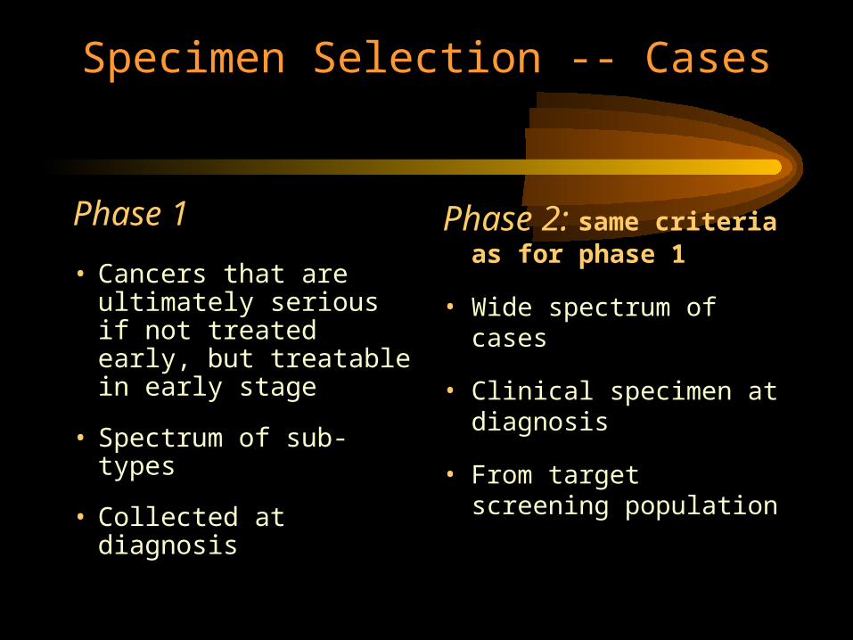
Specimen Selection -- Cases
Phase 1
• Cancers that are ultimately serious if not treated early, but treatable in early stage
• Spectrum of sub-types
• Collected at diagnosis
Phase 2: same criteria as for phase 1
• Wide spectrum of cases
• Clinical specimen at diagnosis
• From target screening population
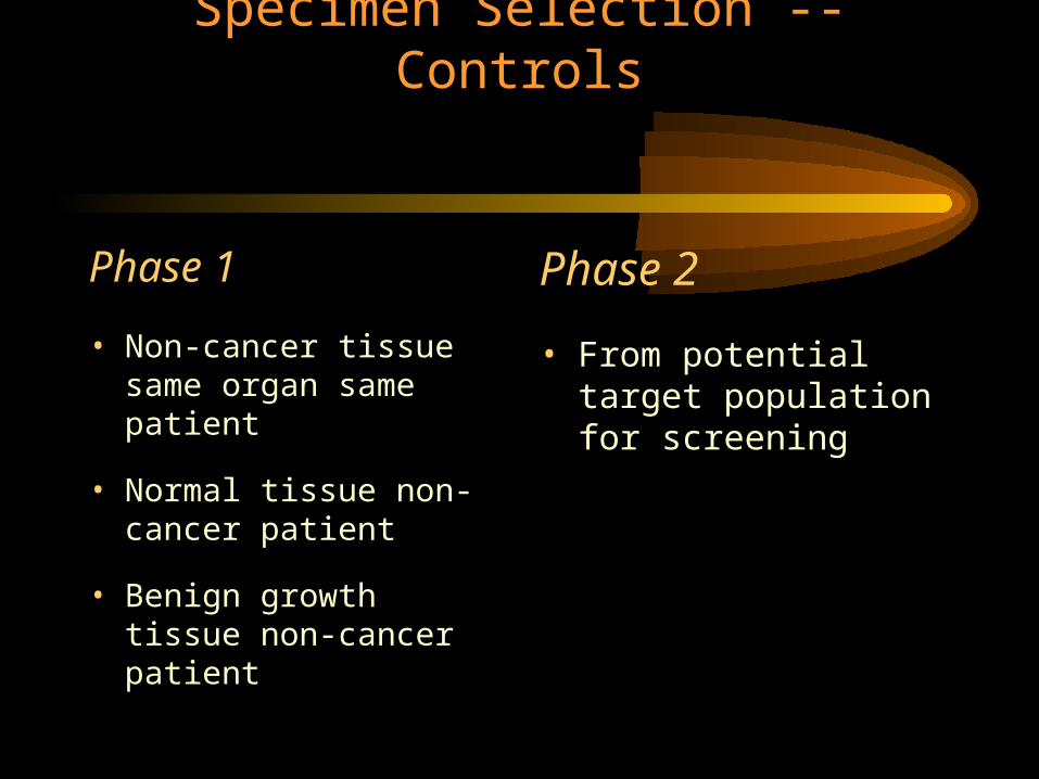
Specimen Selection -- Controls
Phase 1
• Non-cancer tissue same organ same patient
• Normal tissue non-cancer patient
• Benign growth tissue non-cancer patient
Phase 2
• From potential target population for screening

Outcome Measures
Phase 1
• True positive and False positive rates (binary result)
• True positive rate at threshold yielding acceptable false positive rate
• ROC curve
Phase 2
• Results of clinical biomarker assay

Evaluation of Results
Phase 1
• Algorithms select and prioritize markers that best distinguish tumor from non-tumor tissue
• Initial exploratory studies need confirmation with new validation specimens
Phase 2
• ROC curves
• ROC regression to determine if characteristics of cases and/or characteristics of controls effect biomarker’s discriminatory capacity

Sample Size
Phase 1
• Should be large enough so that very promising biomarkers are likely to be selected for phase 2 development
Phase 2
• Based on a confidence intervals for the TPR or FPR, or confidence intervals for the ROC curve at selected critical points
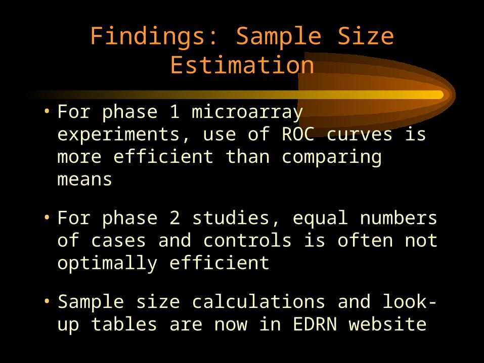
Findings: Sample Size Estimation
• For phase 1 microarray experiments, use of ROC curves is more efficient than comparing means
• For phase 2 studies, equal numbers of cases and controls is often not optimally efficient
• Sample size calculations and look-up tables are now in EDRN website
1. Pepe et al. Phases of biomarker development for early detection of cancer. Journal of the National Cancer Institute 93(14):1054–61, 2001.
2. Pepe et al. “Elements of Study Design for Biomarker Development” In Tumor Markers, Diamandis, Fritsche, Lilja, Chan, and Schwartz , eds. AAAC Press, Washington, DC. 2002.
3. Pepe. “Statistical Evaluation of Diagnostic Tests & Biomarkers” Oxford U. Press, 2003.
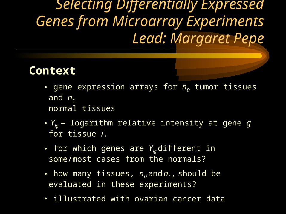
Selecting Differentially Expressed Genes from Microarray Experiments
Lead: Margaret Pepe
Context• gene expression arrays for nD tumor tissues and nC
normal tissues
• Yig = logarithm relative intensity at gene g for tissue i.
• for which genes are Yig different in some/most cases from the normals?
• how many tissues, nD and nC, should be evaluated in these experiments?
• illustrated with ovarian cancer data
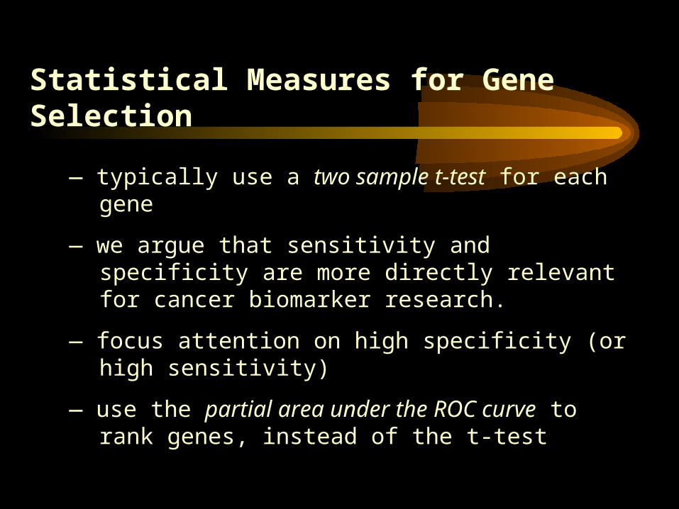
Statistical Measures for Gene Selection
— typically use a two sample t-test for each gene
— we argue that sensitivity and specificity are more directly relevant for cancer biomarker research.
— focus attention on high specificity (or high sensitivity)
— use the partial area under the ROC curve to rank genes, instead of the t-test

Example
Gene Rank (among 100 genes)
gene #5 gene #97
t-test 10 4
partial AUC 3 31
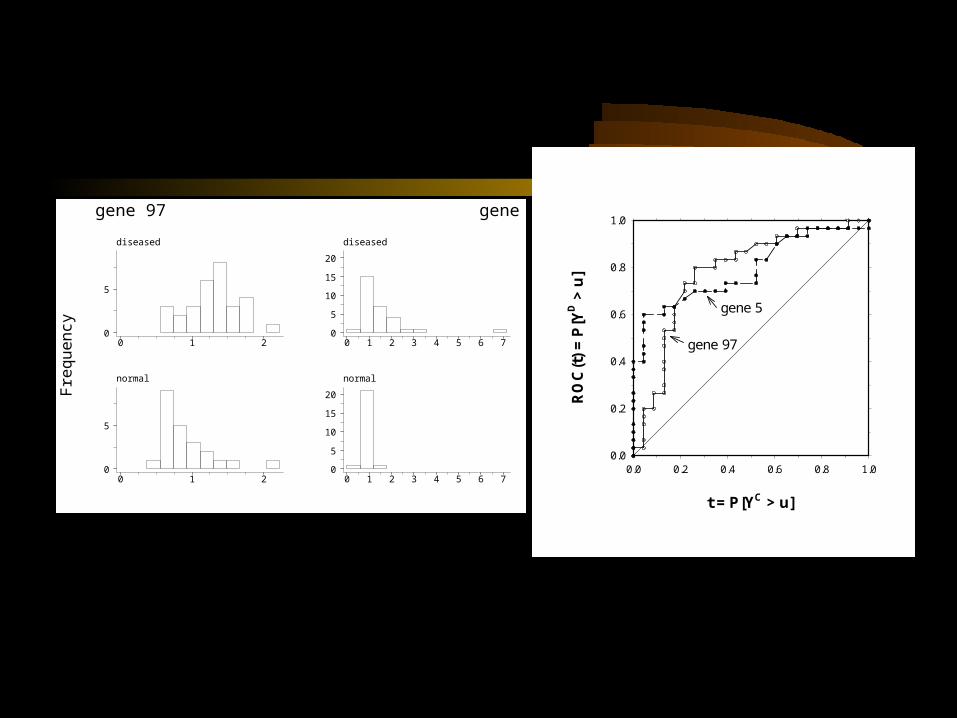
t = P[YC > u]
0.0 0.2 0.4 0.6 0.8 1.0
RO
C(t
) =
P[Y
D >
u]
0.0
0.2
0.4
0.6
0.8
1.0
gene 5
gene 97
F
requ
ency
diseased
0 1 2
0
5
diseased
0 1 2 3 4 5 6 7
0
5
10
15
20
normal
0 1 2
0
5
normal
0 1 2 3 4 5 6 7
0
5
10
15
20
gene 97 gene 5
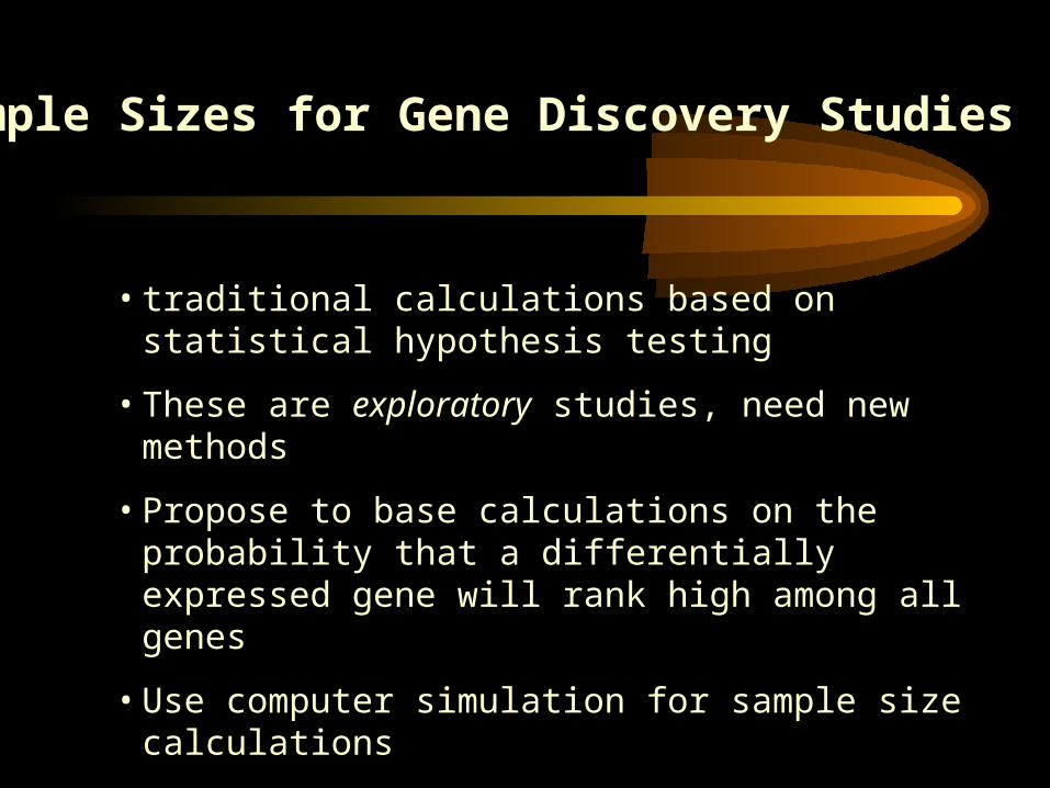
• traditional calculations based on statistical hypothesis testing
• These are exploratory studies, need new methods
• Propose to base calculations on the probability that a differentially expressed gene will rank high among all genes
• Use computer simulation for sample size calculations
Sample Sizes for Gene Discovery Studies
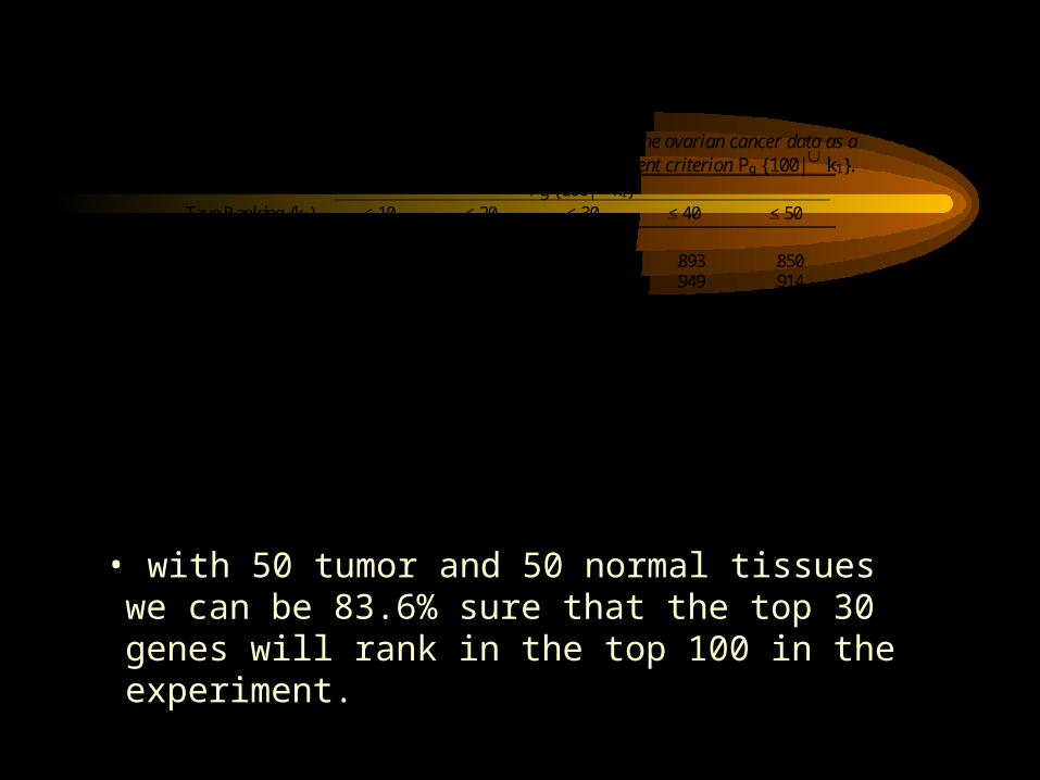
Table 3 Study power Pg {100| k1} as a function of sample size using the ovarian cancer data as a simulation model. Also shown is the power for the more stringent criterion Pg {100| k1}.
Pg {100| k1} True Ranking (k1) < 10 < 20 < 30 < 40 < 50
(nD, nc) (15, 15) .997 .982 .934 .893 .850 (25, 25) 1.000 .996 .973 .949 .914 (50, 50) 1.000 1.000 .994 .987 .968 (100, 100) 1.000 1.000 .999 .998 .990 Pg {100| k1}. (15, 15) .960 .654 .120 .016 .000 (25, 25) 1.000 .928 .486 .202 .024 (50, 50) 1.000 1.000 .836 .638 .206 (100, 100) 1.000 1.000 .984 .928 .608
• with 50 tumor and 50 normal tissues we can be 83.6% sure that the top 30 genes will rank in the top 100 in the experiment.
• Pepe et al. Selecting differentially expressed genes from microarray experiments. Biometrics (in press)
Summary
• The method we developed for selecting genes and calculating sample sizes are more appropriate for the purpose of diagnosis and early detection
Analysis:Statistical Methods for Biomarker Discovery from
High-Dimensional Data Sets
• Method development motivated by SELDI data from John Semmes/George Wright at Eastern Virginia Medical School
• Data consist of protein intensities at tens of thousands of mass/charge points on each of 297 individuals
• Developed three approaches to biomarker discovery: wavelets, boosting decision tree, and automated peak identification

The EVMS prostate cancer biomarker project
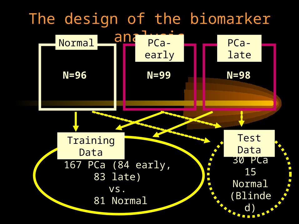
• Prostate cancer patients: N=99 early-stageN=98 late-stage
• Normal controls N=96
• Serum samples for proteomic analysis by Surface Enhanced Laser Desorption/Ionization (SELDI)
• Goal: To discover protein signals that distinguish cancers from normals
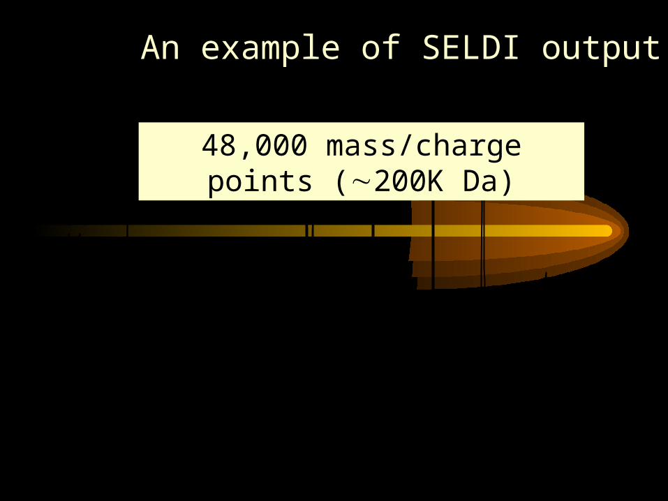
An example of SELDI output
Mass/Charge
Inte
nsity
2000 3000 4000 5000 6000 7000 8000
02
46
8
48,000 mass/charge points (200K Da)
Normal
The design of the biomarker analysisPCa-
earlyPCa-late
N=96
N=99
N=98
Training Data
167 PCa (84 early, 83 late)vs.
81 Normal
Test Data
30 PCa15
Normal(Blinded)

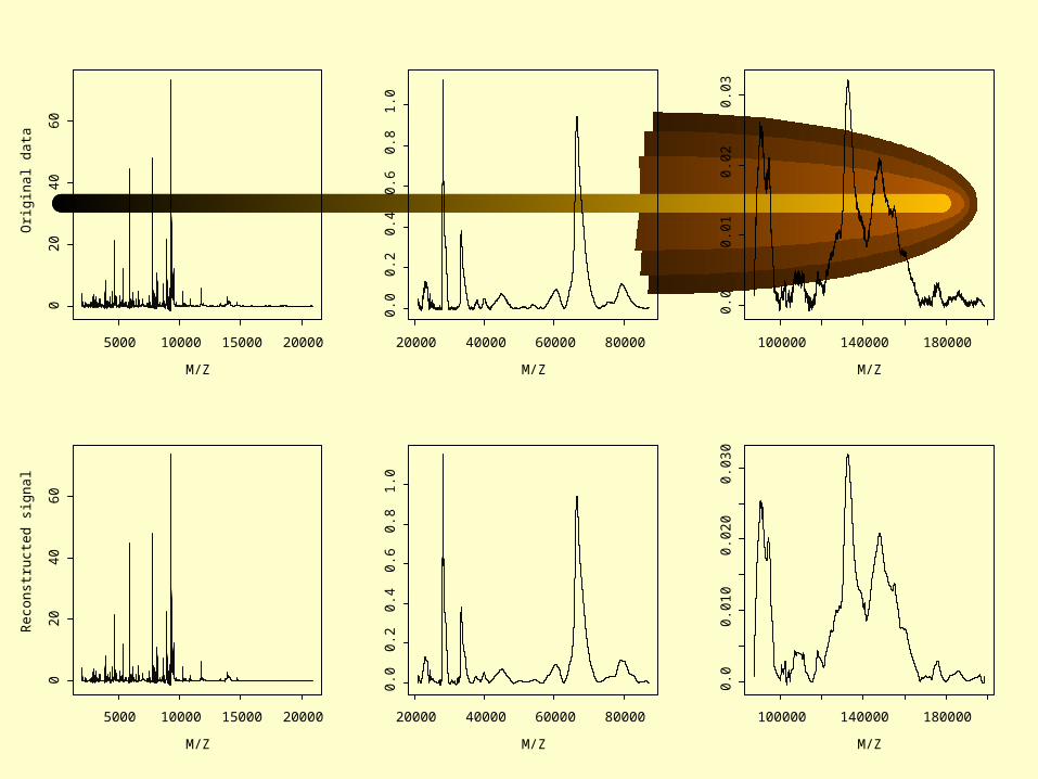
Wavelet AnalysisLead: Yinsheng Qu
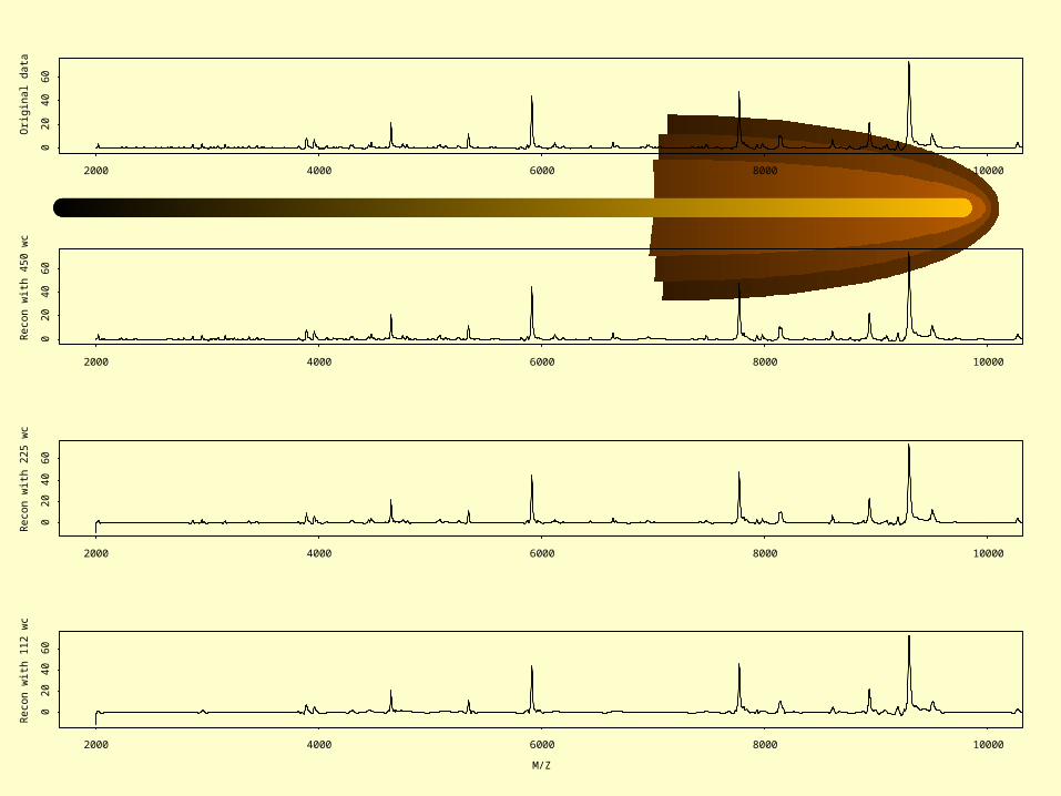
Steps in the wavelet analysis:• Represent original data plot with a set of
wavelets (dimension reduction)• Determine those wavelets that distinguish
between subgroups (information criterion)• Define discriminating functions based on
the distinguishing wavelets (Fisher discrimination)
M/Z
Ori
gin
al d
ata
5000 10000 15000 20000
02
04
06
0
M/Z
20000 40000 60000 80000
0.0
0.2
0.4
0.6
0.8
1.0
M/Z
100000 140000 180000
0.0
0.0
10
.02
0.0
3M/Z
Re
con
stru
cte
d s
ign
al
5000 10000 15000 20000
02
04
06
0
M/Z
20000 40000 60000 80000
0.0
0.2
0.4
0.6
0.8
1.0
M/Z
100000 140000 1800000
.00
.01
00
.02
00
.03
0
Orig
ina
l da
ta
2000 4000 6000 8000 10000
02
04
06
0
Re
con
with
45
0 w
c
2000 4000 6000 8000 10000
02
04
06
0
Re
con
with
22
5 w
c
2000 4000 6000 8000 10000
02
04
06
0
M/Z
Re
con
with
11
2 w
c
2000 4000 6000 8000 10000
02
04
06
0

Three Group Classification:Normal, Cancer, BPH
12,352 mass spectrum data points, reduced to3,420 Haar wavelet coefficients, of which17 coefficients distinguish between the three cases.2 classification functions generated.
Truth:Predicted: Normal Cancer BPHNormal 14 0 0Cancer 1 27 7BPH 0 3 8
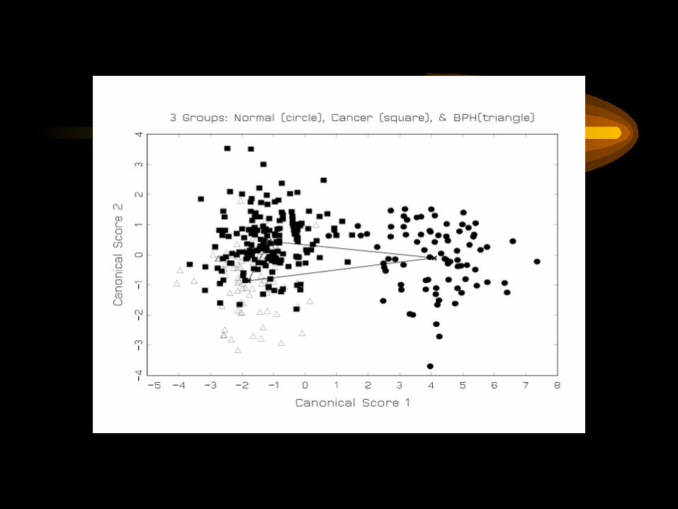
Qu Y et al. Data reduction using discrete wavelet transform in discriminant analysis with very high dimension. Biometrics, in press.
Boosted Decision Tree Method. Lead: Yinsheng Qu/Yutaka Yasui
• This method combines multiple weak learners into a very accurate classifier
• It can be used in cancer detection
• It can also be used in identification of tumor markers
• Using this method we can separate controls, BPH, and PCA without error in test set

Outline of boosting decision tree
• The combined classifier is a committee with the decision stumps, the base classifiers, as its members. It makes decisions by majority vote.
• The base classifiers are constructed on weighted examples: the examples misclassified will increase their weights on next round.
• The 2nd stump’s specialty is to correct the 1st stump’s mistakes, and the 3rd stump’s specialty is to correct the 2nd stump’s mistakes, and so on.
• The combined classifier with dozens and even hundreds of decision stumps will be accurate.
• Boosting technique is resistant to over fitting.

Classifier 2: A boosted decision stump classifier with 21 peaks (potential markers)
Training set Testing set
normal bph cancer normal bph cancer
normal 82 0 0 14 0 1
bph 0 74 3 0 15 0
cancer 7 0 160 0 1 29
sensitivity 95.81% 96.67%
specificity 98.11% 96.67%
# of peaks 21 in 21 base classifiers
minimal margin -0.2555
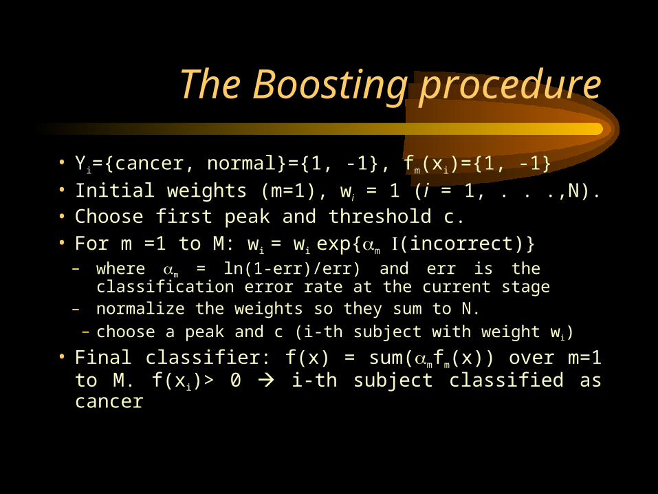
The Boosting procedure
• Yi={cancer, normal}={1, -1}, fm(xi)={1, -1}• Initial weights (m=1), wi = 1 (i = 1, . . .,N). • Choose first peak and threshold c.• For m =1 to M: wi = wi exp{m (incorrect)}
– where m = ln(1-err)/err) and err is the classification error rate at the current stage
– normalize the weights so they sum to N.– choose a peak and c (i-th subject with weight wi)
• Final classifier: f(x) = sum(mfm(x)) over m=1 to M. f(xi)> 0 i-th subject classified as cancer
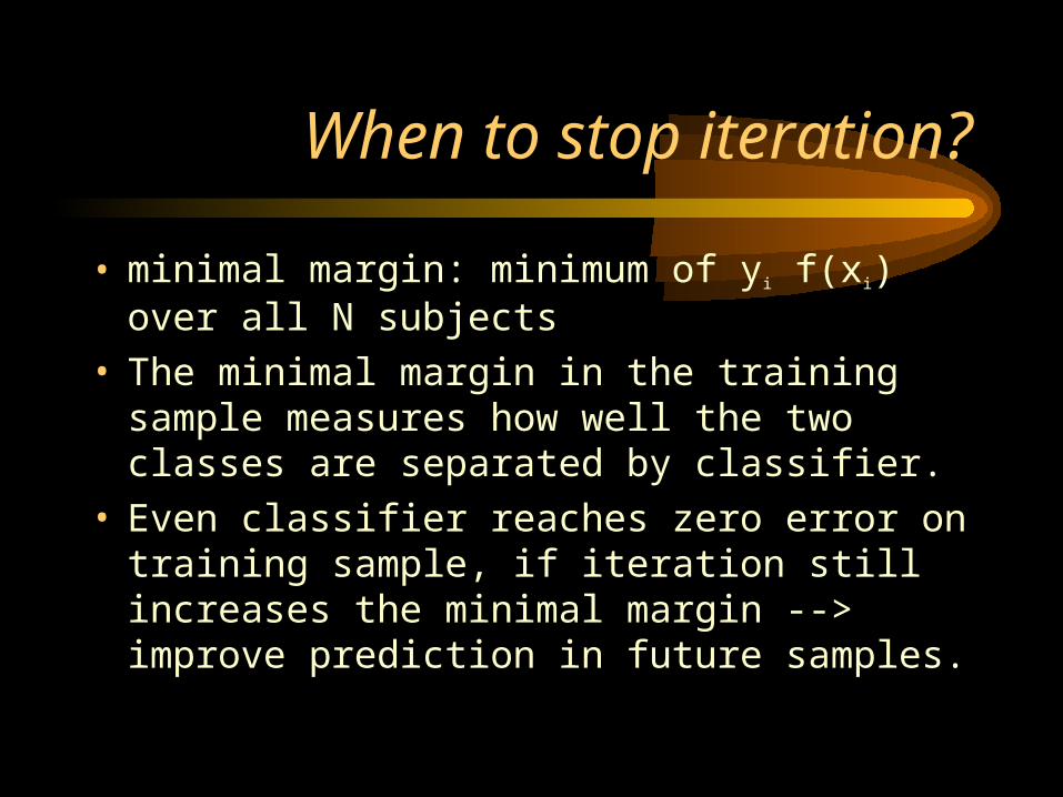
When to stop iteration?
• minimal margin: minimum of yi f(xi) over all N subjects
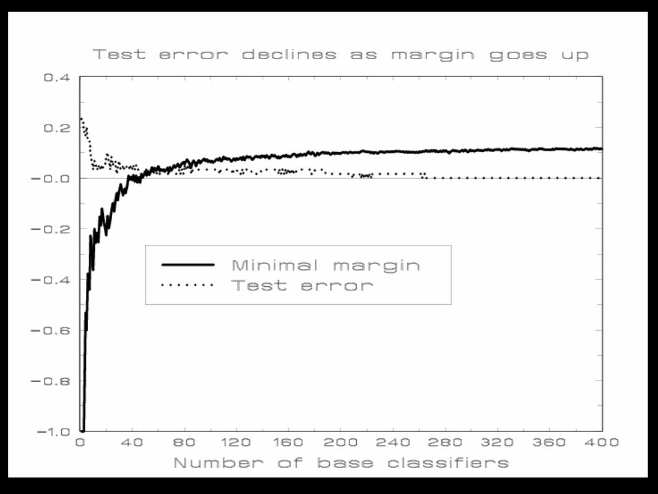
• The minimal margin in the training sample measures how well the two classes are separated by classifier.
• Even classifier reaches zero error on training sample, if iteration still increases the minimal margin --> improve prediction in future samples.
• Qu et al. 2002. Boosted Decision Tree Analysis of SELDI Mass Spectral Serum Profiles Discriminates Prostate Cancer from Non-Cancer Patients. Clinical Chemistry. In press.
• Adam et al. 2002. Serum Protein Fingerprinting Coupled with a Pattern Matching Algorithm that Distinguishes Prostate Cancer from Benign Prostate Hyperplasia and Healthy Men. Cancer Research. 62:3609-3614.
Summary
• Wavelets approach: Does not require peak identification (black-box classification)
• Boosting decision tree: Requires peak identification first. Useful for both classification and protein mass identification
Final Summary
• The methods developed in the past two years are mainly for Phase 1&2 studies, reflecting the current needs of EDRN.
• EDRN DMCC statisticians are working on key design and analysis issues in early detection research.
• More work remains to be done (e.g., In classification, consider the mislabeling of Prostate cancer by BPH; exam gene by environmental interactions).