Stated-preference study to examine the economic value...
113
1 Stated-preference study to examine the economic value of benefits of avoiding selected adverse human health outcomes due to exposure to chemicals in the European Union Service contract for the European Chemicals Agency No. ECHA/2011/123 Part I: sensitization & dose toxicity Charles University in Prague (Environment Center) VU University Amsterdam (Faculty of Earth and Life Sciences) August 2014 (revised November 2014)
Transcript of Stated-preference study to examine the economic value...

1
Stated-preference study to examine the economic
value of benefits of avoiding selected adverse human health outcomes due to exposure to
chemicals in the European Union
Service contract for the European Chemicals Agency No. ECHA/2011/123
Part I: sensitization & dose toxicity
Charles University in Prague (Environment Center)
VU University Amsterdam (Faculty of Earth and Life Sciences)
August 2014 (revised November 2014)

Stated-preference study to examine the economic value of benefits of avoiding selected adverse human health outcomes due to exposure to chemicals in the European Union – Part 1
2

Stated-preference study to examine the economic value of benefits of avoiding selected adverse human health outcomes due to exposure to chemicals in the European Union – Part 1
3
Table of Contents
0. Executive summary ......................................................................................................................... 9
1. Introduction ................................................................................................................................... 13
Skin and respiratory health effects of sensitizers .................................................................. 13 1.1.
Dose toxicity to kidneys ........................................................................................................ 14 1.2.
2. Review of valuation studies........................................................................................................... 15
Skin sensitization ................................................................................................................... 15 2.1.
Respiratory sensitization ....................................................................................................... 16 2.2.
Dose toxicity .......................................................................................................................... 18 2.3.
Health outcomes chosen for survey ....................................................................................... 19 2.4.
3. Methods ......................................................................................................................................... 21
Contingent valuation ............................................................................................................. 21 3.1.
3.1.1. Choice CVM elicitation format .........................................................................................21
3.1.2. Elicitation method chosen for the study .............................................................................24
Econometric modelling of WTP ............................................................................................ 24 3.2.
3.2.1. Non-parametric modelling of interval WTP data ..............................................................24
3.2.2. Parametric modelling .........................................................................................................25
3.2.3. Testing of model validity ...................................................................................................26
3.2.4. Joint estimation of WTP for avoiding outcomes with varying attributes ..........................26
Standard gamble with chaining ............................................................................................. 27 3.3.
4. Questionnaire and survey .............................................................................................................. 29
Questionnaire structure .......................................................................................................... 29 4.1.
4.1.1. Current health state, illness introduction and rating ..........................................................29
4.1.2. Contingent valuation ..........................................................................................................30
4.1.3. Standard gamble ................................................................................................................31
4.1.4. Socio-economic characteristics and debriefing..................................................................32
Survey design ........................................................................................................................ 32 4.2.
4.2.1. Pre-survey and pilot ...........................................................................................................32
4.2.2. Sampling strategy ..............................................................................................................33
5. Data description ............................................................................................................................. 34
Data clearing and identification of potential speeders ........................................................... 34 5.1.
Non-response analysis ........................................................................................................... 35 5.2.
Quota variables ...................................................................................................................... 37 5.3.
Country samples descriptive statistics and health state assessments ..................................... 38 5.4.

Stated-preference study to examine the economic value of benefits of avoiding selected adverse human health outcomes due to exposure to chemicals in the European Union – Part 1
4
5.4.1. Health conditions of respondents and their relatives .........................................................41
5.4.2. Respondents’ health state self-assessment .........................................................................41
5.4.3. Health care systems and the coverage ...............................................................................43
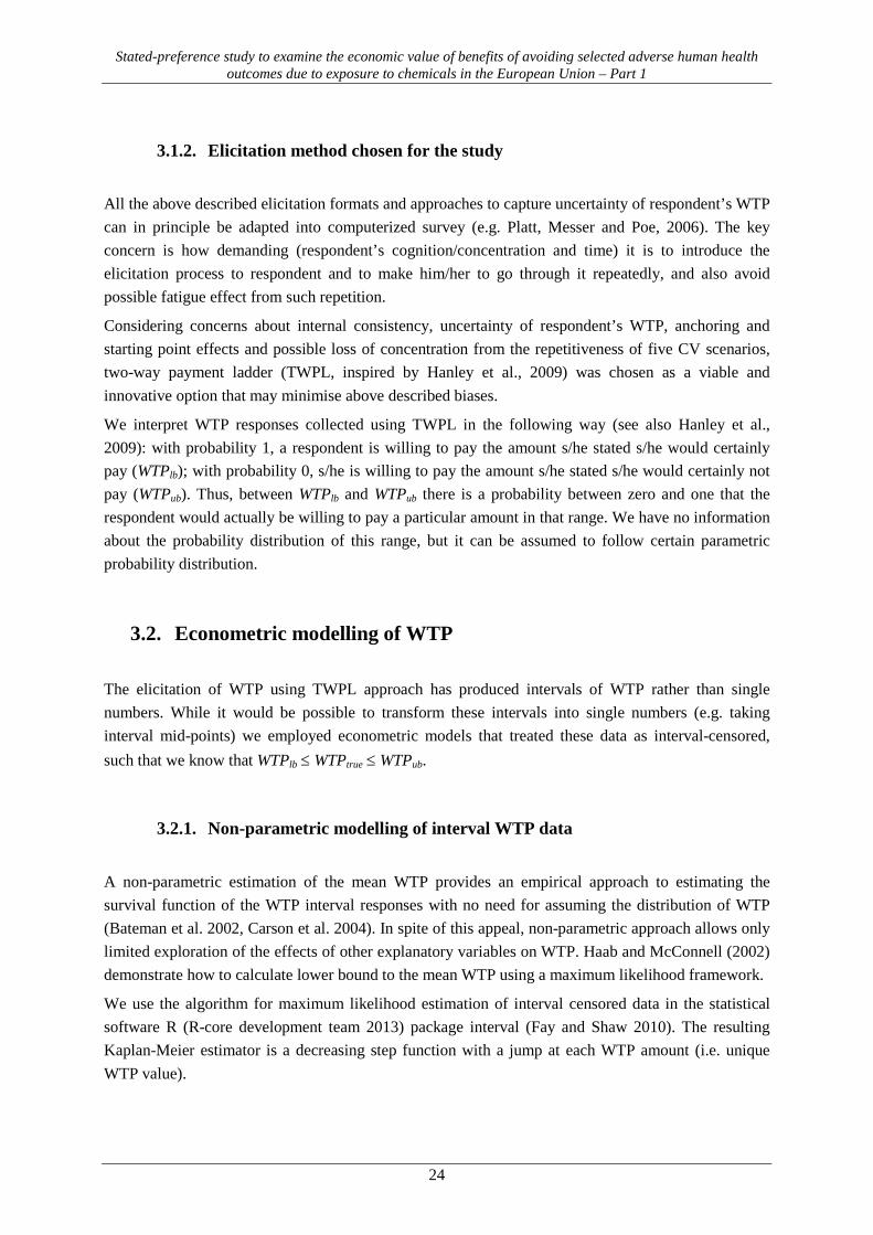
5.4.4. Perception of health risks of chemicals in consumer products ..........................................44
Research design and its distribution ...................................................................................... 47 5.5.
Debriefing - content validity of the CVM and comprehensibility ......................................... 47 5.6.
6. WTP estimates ............................................................................................................................... 51
Identification of true and protest zeros .................................................................................. 51 6.1.
Identification of outliers ........................................................................................................ 55 6.2.
Non-parametric WTP estimates ............................................................................................ 56 6.3.
Parametric WTP estimates .................................................................................................... 60 6.4.
6.4.1. Validity test ........................................................................................................................62
6.4.2. Joint estimation of WTP for avoiding illnesses A through A3 ..........................................69
6.4.3. Income elasticity of WTP ..................................................................................................71
Standard gamble with chaining ............................................................................................. 72 6.5.
7. Health rating and QALY ............................................................................................................... 78
8. Benefit transfer .............................................................................................................................. 81
PPP-adjusted unit value transfer ............................................................................................ 81 8.1.
Sensitivity analysis ................................................................................................................ 82 8.2.
9. Discussion ..................................................................................................................................... 84
Comparison with other studies/estimates .............................................................................. 84 9.1.
Scope sensitivity .................................................................................................................... 85 9.2.
9.2.1. Diminishing marginal value of skin sensitization episode .................................................88
Speeders................................................................................................................................. 90 9.3.
10. Conclusions ............................................................................................................................... 91
11. References ................................................................................................................................. 95
12. Appendices .............................................................................................................................. 101

Stated-preference study to examine the economic value of benefits of avoiding selected adverse human health outcomes due to exposure to chemicals in the European Union – Part 1
5
List of tables
Table 1 – EU-wide WTP values for health outcomes ............................................................................. 9 Table 2 – Overview of illness A(x) variants appearing in contingent valuation ................................... 30 Table 3 – Overview of health outcomes appearing in standard gamble ................................................ 31 Table 4 - Sample sizes and return rates for CAWI ................................................................................ 34 Table 5 – Share of potential speeders in answering the online questionnaire (for respondents in the main wave only) .................................................................................................................................... 34 Table 6 – non-response tests ................................................................................................................. 35 Table 7 – Quota variables - descriptive sample and population statistics ............................................. 37 Table 8 – Age by country ...................................................................................................................... 37 Table 9 – Education by country – highest level achieved ..................................................................... 38 Table 10 - Total monthly household income by country ....................................................................... 38 Table 11 - Descriptive sample and population statistics ....................................................................... 39 Table 12 – Marital status (sample) ........................................................................................................ 39 Table 13 – Number of children in respondent’s household (18 years or below) .................................. 39 Table 14 – Economic status ................................................................................................................... 40 Table 15 - Total monthly personal income by country ......................................................................... 40 Table 16 – Respondent’s diagnoses ...................................................................................................... 41 Table 17 - Diagnoses of respondent’s household members, relatives, close friends ............................ 41 Table 18 – Assessment of health states – mean values from Visual Analogue Scales ......................... 43 Table 19 – Type of health insurance by country ................................................................................... 43 Table 20 – Coverage of respondent’s health care: the prescribed drugs needed ................................... 44 Table 21 – Coverage of respondent’s health care: in-patient health care in hospital or clinic .............. 44 Table 22 – Share of “I don’t use/not relevant” answer.......................................................................... 45 Table 23 – Frequency of variants of the factorial design ...................................................................... 47 Table 24 – Agreement with the statement: “I can easily imagine such a payment decision.” ............ 47 Table 25 – Most difficult illnesses to value ........................................................................................... 48 Table 26 – Reasons for difficulty to value the illnesses ........................................................................ 48 Table 27 – Share of respondents who do not consider paying for avoiding illness (i.e. zero WTP) ..... 51 Table 28 – Share of protesting respondents (i.e. protest zero WTP) ..................................................... 52 Table 29 - Most important reasons for refusal of paying to avoid Illness A (acute mild dermatitis) .... 53 Table 30 - Most important reasons for refusal of paying to avoid Illness A1 (mild dermatitis – 1 year; 2 or 4 times) ........................................................................................................................................... 53 Table 31 - Most important reasons for refusal of paying to avoid Illness A2 (mild dermatitis – 2, 5, 10 years) ..................................................................................................................................................... 53 Table 32 - Most important reasons for refusal of paying to avoid Illness A3 (mild dermatitis) ........... 54 Table 33 - Most important reasons for refusal of paying to avoid Illness C (acute kidney injury) ....... 54 Table 34 – Respondents excluded as outliers ........................................................................................ 56 Table 35 - WTP for avoiding illnesses (truncation strategy I, non-parametric estimates, in “generic” euro/case) .............................................................................................................................................. 58 Table 36 - WTP for avoiding illnesses (truncation strategy II, non-parametric estimates, in euro/case) ............................................................................................................................................................... 59 Table 37 - Definition and descriptive statistics of explanatory variables .............................................. 62

Stated-preference study to examine the economic value of benefits of avoiding selected adverse human health outcomes due to exposure to chemicals in the European Union – Part 1
6
Table 38 - Parametric model of zero WTP (part 1 model) and positive WTP (part 2 model) for avoiding illness A (acute dermatitis) ..................................................................................................... 64 Table 39 - Parametric model of zero WTP (part 1 model) and positive WTP (part 2 model) for avoiding illness A1 (dermatitis: 2x or 4x) ............................................................................................. 65 Table 40 - Parametric model of zero WTP (part 1 model) and positive WTP (part 2 model) for avoiding illness A2 (dermatitis: once a year over 2, 5, or 10 years) ..................................................... 66 Table 41 - Parametric model of zero WTP (part 1 model) and positive WTP (part 2 model) for avoiding illness A3 (dermatitis: 2x or 4x a year over 2, 5, or 10 years)................................................ 67 Table 42 - Parametric model of zero WTP (part 1 model) and positive WTP (part 2 model) for avoiding illness C (acute kidney injury) ................................................................................................ 68 Table 43 – Regression models for joint estimation of WTP for avoiding illnesses A through A3 ....... 69 Table 44 – Estimated WTP income elasticities ..................................................................................... 71 Table 45 - Accepted chances of new treatment failure in 1st standard gamble (means of intervals’ mid-points) .................................................................................................................................................... 73 Table 46 – Accepted chances of new treatment failure in 2nd and 3rd standard gamble (means of intervals’ mid-points) ............................................................................................................................ 74 Table 47 - Implicit WTP for avoiding health endpoints (in EUR per case, PPP-corrected) ................. 77 Table 48 – health assessments of current health vs. illnesses A through D .......................................... 79 Table 49 – annual QALY losses ............................................................................................................ 79 Table 50 – Mean EU28-wide WTP values (in EUR, population weighted mean) ................................ 81 Table 51 – Mean EU28-wide WTP values for sensitivity analysis (in EUR, no population weighting) ............................................................................................................................................................... 82 Table 52 - Error rates of benefit transfer ............................................................................................... 82 Table 53 – Number of respondents with the same WTP for avoiding illness A and another illness .... 85 Table 54 - Effect of excluding insensitive respondents on WTP .......................................................... 86 Table 55 - Number of respondents who have stated the same WTP for avoiding all the illnesses ....... 86 Table 56 – Internal scope tests (Wilcoxon two-sample tests) ............................................................... 87 Table 57 - External scope tests (Wilcoxon two-sample/trend tests)...................................................... 87 Table 58 – Internal proportional scope test ........................................................................................... 88 Table 59 – Mean EU-wide WTP values for health outcomes (WTP per case, in EUR2012) .................. 93
List of figures
Figure 1 - Illness A (acute sensitisation) ............................................................................................... 19 Figure 2 - Illness B (chronic sensitisation) ............................................................................................ 19 Figure 3 - Illness C (acute kidney injury) .............................................................................................. 20 Figure 4 - Illness C (chronic kidney disease) ........................................................................................ 20 Figure 5 – Standard gamble experiment ................................................................................................ 27 Figure 6 – Two-way payment ladder ..................................................................................................... 30 Figure 7 – Tree of risks used in standard gambles ................................................................................ 31 Figure 8 – number of respondents answering subsequent parts of the questionnaire (those who did not complete the questionnaire) ................................................................................................................... 36 Figure 9 – Mean assessment of health states (VAS) ............................................................................. 42 Figure 10 – Mean assessment of health states (VAS) for individual countries ..................................... 42

Stated-preference study to examine the economic value of benefits of avoiding selected adverse human health outcomes due to exposure to chemicals in the European Union – Part 1
7
Figure 11 – Worries about the potential risk to health that may arise from the chemicals present in the following products ................................................................................................................................. 45 Figure 12 – Health risks believed to arise from chemicals in household products (%) ........................ 46 Figure 13 – Importance of characteristics of the illness ........................................................................ 49 Figure 14 – Consideration when stating WTP ...................................................................................... 49 Figure 15 – Nonparametric estimates of mean and median WTP for avoidance of individual illnesses ............................................................................................................................................................... 57 Figure 16 - Nonparametric estimates of mean and median WTP (truncation strategy II, pooled) ........ 59 Figure 17 – Parametric estimates of mean and median WTP for avoidance of individual illnesses ..... 60 Figure 18 - Parametric estimates of mean WTP (truncation strategy II, pooled) .................................. 62 Figure 19 – Changes in WTP relative to duration of sensitization episodes ......................................... 70 Figure 20 – Changes in WTP relative to frequency of sensitization episodes ...................................... 71 Figure 21 – Kaplan-Meier non-parametric estimators of distribution of minimum new treatment success in each standard gamble ........................................................................................................... 72 Figure 22 – Kaplan-Meier non-parametric estimators of distribution of minimum new treatment success in SG-1 sub-variants ................................................................................................................. 73 Figure 23 – Mean accepted chance of new treatment success .............................................................. 75 Figure 24 – ratio of implied WTP for a single sensitization episode in illness profiles A1, A2 and A3 vs WTP for illness A ............................................................................................................................. 89
List of abbreviations
CVM – contingent valuation method
DCU – dichotomous choice uncertainty
ESRD – end-stage renal disease
GSCE – General Certificate of Secondary Education
HICP – harmonised index of consumer prices
ICD – International classification of illnesses
MBU – multiple bounded uncertainty
NUTS – Nomenclature of Units for Territorial Statistics
PPP – purchasing parity power
QALY – Quality-adjusted life year
SG – standard gamble
SVHC – substances of very high concerns
TTO – time trade-off
TWPL – two-way payment ladder
VAS – visual analogue scale
WTP – willingness-to-pay

Stated-preference study to examine the economic value of benefits of avoiding selected adverse human health outcomes due to exposure to chemicals in the European Union – Part 1
8

Stated-preference study to examine the economic value of benefits of avoiding selected adverse human health outcomes due to exposure to chemicals in the European Union – Part 1
9
0. Executive summary
The primary objective of this stated-preference study was two-fold: (1) to estimate willingness to pay to avoid selected adverse human health outcomes due to exposure to chemicals in the European Union, and (2) to derive representative EU-wide benefit estimates reference values that ECHA and other bodies can use when carrying out socio-economic analyses or health impact assessment in connection with REACH Regulation. This report focuses on skin sensitization and dose toxicity that were dealt with in the first survey conducted within the study.
Based on a literature review and in close cooperation with ECHA, the following health outcomes related to skin sensitization and dose toxicity were selected for the valuation survey: mild acute dermatitis (including the effect of repeated episodes), severe chronic dermatitis, acute kidney injury and chronic kidney disease. Respective willingness-to-pay values were elicited from an adult population sample in four EU Member States: the Czech Republic, the United Kingdom, the Netherlands and Italy using a combination of contingent valuation method (CVM) and standard gamble with chaining approach. Two-way payment ladder was applied for elicitation of WTP discrete intervals.
The data collected were cleaned for speeders, protesters and outliers (with alternative truncation strategies for identification of outliers). Based on (purchasing power adjusted-) unit value transfer from a model of WTP from interval data, the following EU-wide benefit values were derived from non-parametric estimates based on two truncation strategies for the respective health outcomes.
Table 1 – EU-wide WTP values for health outcomes
health outcome WTP per case (EUR2012)
truncation strategy I truncation strategy II
acute mild dermatitis 227 222
episodes of acute mild dermatitis (4 over one year) 329 295
episodes of acute mild dermatitis (1/yr. over 5 years) 352 292
episodes of acute mild dermatitis (4/yr. over 10 years) 615 473
chronic dermatitis 1,055 908
acute kidney injury 532 473
chronic kidney disease 2,761 2,375
The main findings from the valuation study can be summarized as follows:
i) About 3.6% of the respondents completed the questionnaire below 48% of the median time for completion and were labelled potential ‘speeders’. Subsequent analysis shows that these respondents were insensitive to the severity of health states presented, i.e. expressed statistically indifferent willingness to pay for acute mild dermatitis and acute kidney injury.
ii) The share of respondents who did not express a positive willingness to pay was between 13% and 16% of the sample. Of those who did not express a positive willingness to pay, between 58% and 76% are classified as protest zeros, i.e. they state zero WTP because they protest at

Stated-preference study to examine the economic value of benefits of avoiding selected adverse human health outcomes due to exposure to chemicals in the European Union – Part 1
10
one or more aspects of the CV scenario. Protesters and speeders were excluded from the sample before calculating mean and median WTP.
iii) The highest share of protesters is consistently found in the Netherlands – between 9% for mild dermatitis and 15% for acute kidney injury – and the lowest in the Czech Republic – between 7% and 9%.
iv) The highest share of respondents not willing to pay anything is consistently found in the Netherlands (around one fifth of the sample) and the lowest in the Czech Republic over all the endpoints.
v) There are considerable differences in WTP between countries. Willingness to pay is consistently higher in Italy than in the remaining countries across all illnesses and all types of models.
vi) Parametric models yield WTP estimates that are not systematically higher than non-parametric estimates across all illnesses. Non-parametric estimates are slightly lower than the parametric estimate for avoiding milder health outcomes. In the case of 6 variants of repeated mild dermatitis (Illness A3) parametric WTP estimates are higher than non-parametric estimates in 4 variants (based on a truncation strategy I).
vii) The influence of alternative strategies to identify and exclude likely implausible WTP values (outliers) on measures of central tendency is mixed – while mean WTP values decreased between 2-30% (non-parametric) or up to 14% (parametric estimates), median WTP values remained almost unchanged.
viii) We found a consistently declining marginal value of additional skin sensitization episode in illnesses with repeated sensitization episodes to corroborate the assumption of economic theory.
ix) The coefficient of interaction term in the joint estimation of WTP for avoiding repeated mild dermatitis is negative, suggesting that WTP for more frequent and longer lasting episodes is not a simple sum of WTP for individual episodes.
x) The elicited WTP values for variants of the acute dermatitis profile seem inadequately sensitive to the quantity of episodes avoided offered in the hypothetical market (scope effect). Scope insensitivity was rejected in 20 out of 32 internal scope tests and all external scope tests. We find that the marginal value of an additional skin sensitisation episode consistently declines with increasing number of episodes in illness profile (cf. Figure 24). The estimated models of WTP are internally valid – in particular, income is found to be a significant and positive predictor of WTP as suggested by economic theory.
xi) The estimated WTP values for avoiding acute dermatitis are relatively high compared to valuation of other milder morbidity symptoms, but generally meaningful compared e.g. to the value of a symptom day Ready et al. study (2004) (EUR2012 70). Also, a sharply diminishing value of additional sensitisation episode seems to be consistent with several previous studies. The WTP for avoiding acute kidney injury is about twice the WTP for avoiding acute dermatitis, perhaps reflecting more duration than severity. The non-parametric estimate is relatively close to the value of hospital admission in Ready et al. study (2004) (EUR2012 615).
xii) The WTP estimates for the two chronic health outcomes – chronic dermatitis and chronic kidney disease – should be treated with caution. The results tend to indicate that people have preferences for avoiding these illnesses, and are willing to pay more for avoiding more severe illnesses, but these preferences are not very detailed. Hence we observe that implicit WTP for

Stated-preference study to examine the economic value of benefits of avoiding selected adverse human health outcomes due to exposure to chemicals in the European Union – Part 1
11
avoiding chronic kidney disease is only three times the WTP for avoiding acute kidney injury that is presented as an episode lasting only one month. Perhaps the most intuitive explanations would be that respondents either heavily discount their future well-being (what may be – at least in part – compatible with economic theory) or find it difficult to cope with such a hypothetical decision and resort to simplifying heuristics.
xiii) The income elasticities of WTP (calculated as gross impact of income) are at the lower end of the range of estimates found in the literature, between 0.25 for avoiding acute mild dermatitis to 0.35 for avoiding acute kidney injury (using pooled data), but generally increasing with disease severity.
xiv) For the least severe illness – acute mild dermatitis – the income elasticity of WTP is not significantly different from zero for the Dutch respondents and it is also very low for acute kidney injury in the same country sample.
xv) Aside from WTP, loss of health utility was estimated by means of Visual Analogue Scales for four health outcomes – acute mild and chronic severe dermatitis, and acute and chronic disease failure. The derived QALY losses correspond to 0.008, 0.38, 0.028 and 0.558, respectively, and these estimates are broadly comparable with the ranges identified for comparable health outcomes in the literature review.

Stated-preference study to examine the economic value of benefits of avoiding selected adverse human health outcomes due to exposure to chemicals in the European Union – Part 1
12

Stated-preference study to examine the economic value of benefits of avoiding selected adverse human health outcomes due to exposure to chemicals in the European Union – Part 1
13
1. Introduction
A growing concern of European society about the perceived hazards of chemicals to human health and environment has been echoed in the adoption of EC Regulation 1907/2006 (REACH) that substantially reorganized chemicals safety regulation in the EU. The primary goals of REACH is to: (1) compile physicochemical, toxicological, and eco-toxicological data for relevant substances, (2) establish safe usage parameters by means of chemical safety assessments, (3) allow for regulatory evaluation to determine potential hazards, (4) prevent the use of substances of very high concerns (SVHC) without approval by ECHA, and (5) restrict the use of chemicals for which no safe usage parameters can be established. 1
This study aims to provide economic value of benefits that can be used for evaluation of authorisation applications and restriction proposals under the REACH Regulation. This is particularly relevant for analyses of socioeconomic impacts of using SVHC and suitable alternatives that may be a part of authorization application, and analysis of socioeconomic impacts of proposed restriction of substances deemed to hazardous to be used safely as prescribed by Annex XVI.
Skin and respiratory health effects of sensitizers 1.1.
The widespread use of sensitizing substances that also include high volume production substances may pose a substantial societal burden as it is capable of causing allergic reactions in large number of subjects in both working and general population (Burg & Jongeneel, 2011). The health effects of sensitizers range from relative mild to very severe symptoms. Atopic dermatitis, allergic and irritant contact dermatitis, chloracne, hyperkeratosis, coughing, asthma and chronic obstructive pulmonary disease are the examples of these health effects due to exposures to wide range of sensitizers, including antiseptics, aromatic amines, cement, dyes, formaldehyde, artificial, fertilizers, cutting oils, fragrances, glues, lanoline, latex, metals, pesticides, potassium dichromate, preservatives (Prüss-Ustün, Vickers, Haefliger, & Bertollini, 2011). Cosmetics, toys, detergents, clothing and textile and scented products are deemed to pose highest impact/risk for consumers from sensitizing substances such as metals (nickel, cobalt, potassium dichromate), fragrances, (hair) dyes, preservatives and resin/solvents (Burg & Jongeneel, 2011).
The severity of the health effects of sensitizers may differ significantly in the affected population, ranging from situations where subjects sometimes do not even notice any symptoms to situations where medical treatment is necessary. At first, sensitisation effects may be hardly noticeable or even recognized as an allergic effect, since the symptoms often do not occur immediately. A danger lies in such a lack of awareness in that the effects can progress to more severe effects if the exposure is prolonged or repeated once the subject has become sensitive to the allergen in question. Although health effects may subside once exposure has ceased, the allergy remains and cannot be cured; possibly leading to health effects upon every next contact.
The effects of sensitizers go beyond health effects alone. The health effects of sensitizers may lead to socio-economic effects as well. Respiratory and/or skin allergens may hamper persons in their daily 1 For a detailed overview of EU REACH regulation see e.g. Williams et al. (2009).

Stated-preference study to examine the economic value of benefits of avoiding selected adverse human health outcomes due to exposure to chemicals in the European Union – Part 1
14
activities, cause inconveniences, and may also lead to absenteeism of work and change in jobs, because of the recurring effects. Unlike the worker situation, consumers can take actions to avoid contact with an agent provided that the agent is known. However, certain agents, like pollen, are difficult to avoid. Treatment related costs can become very high as the health effects are incurable and treatment is only palliative (symptom based). Costs to society, including implications for workers and consumers, were calculated to be around €29 billion in Europe in 1997 (Diel, Fischer, Kamsteeg, Schubert, & Weber, 2006).
Causal relationships between a chemical agent in sensitizing substances and the clinical effects are difficult to establish since the toxicological mechanisms of sensitization are complex and identification of sensitizing substances can be troublesome (Burg & Jongeneel, 2011).
Dose toxicity to kidneys 1.2.
The kidneys vital function rests in maintaining human health by biotransformation of toxicants and their elimination through excretion of metabolic waste. Damage to the kidneys can affect most organ systems in the body, primarily due to failure of blood filtering and fluid retention. The kidneys can be seriously affected by a number of primary diseases such as hypertension and diabetes, and as evidenced through occupational exposure, poisoning and exposure to heavy metals such as lead, cadmium, and mercury, as well as certain organic solvents (tetrachloromethane, trichloroethylene a toluene), paints, PAHs and further chemicals as analgesics, lithium or cyclosporine has also been shown to be nephrotoxic. For several contaminants, kidney disease is either the critical health effect or one of several prevalent health effects resulting from inhalation, oral, or dermal exposure (US EPA, 2000). EPA´s analysis has identified nine contaminants of concern for hazardous waste management identified to be the critical effect for kidney disease. These include: cadmium, pentachlorophenol, methylene chloride, toluene, pyrene, fluoranthene, ethylbenzene, nitrobenzene, and pentachlorobenzene.
One of the most common manifestations of nephrotoxic damage is acute kidney injury, a sudden loss of the ability of kidneys to remove waste and concentrate urine. Abrupt decline of glomerular filtration rate is mostly a consequence of tubular obstruction or damage and/or increased renal vascular resistance.
Progressive deterioration of renal function may occur with long-term exposure to a variety of chemicals leading to chronic disease, although the underlying mechanisms are not precisely known. Chronic kidney disease is a slow loss of kidney function over time. Final stage of chronic kidney disease is called end-stage renal disease. US incidence is about 2 in 1,000.
US EPA (op. cit.) identify that kidney disease is a debilitating condition that causes numerous adverse physical and emotional conditions of varying severity. People suffering from the disease experience increased morbidity, including mobility effects, muscle cramps, hypertension, or infections. Kidney disease can therefore have a range of lifestyle impacts, including diet changes, daily schedule disruption, and sleep disturbance. It may also cause an increase in emotional stress, resulting in depression, anxiety, pain, loss of energy, and changes in their social relationships. Permanent renal damage may result, requiring chronic dialysis treatment or kidney transplantation.

Stated-preference study to examine the economic value of benefits of avoiding selected adverse human health outcomes due to exposure to chemicals in the European Union – Part 1
15
2. Review of valuation studies
Skin sensitization 2.1.
The literature review did not found any study directly focusing on WTP for avoiding skin sensitisation from chemicals. A few studies exist that address various skin conditions (atopic dermatitis, atopic eczema, psoriasis, melasma, port wine stains, actinic keratosis and alopecia) that may provide some insight on attributes and characteristics that have significant influence on WTP and perception of treatment. These studies, originating mostly from Europe and health economics domain, tend to value less onerous treatments and along with WTP elicit also change in health utility using quality of life instruments.
Lundberg et al. (1999) found that WTP for cure is correlated with Dermatology Life Quality Index (DLQI) and disease activity but not with general quality of life index SF-36. The authors suggest that one possible explanation is that WTP measured only the effect of skin diseases on quality of life than the general measures of quality of life (alternative explanation is a measurement error). Interestingly, the authors note that 3 measures of health state utility – standard gamble, SF-36 and WTP – yielded systematically different results.
Monzini et al. (2006) investigated WTP for different characteristics of atopic dermatitis treatment among dermatitis patients and found that respondents’ WTP for avoiding side effects is second only to duration of therapeutic response. In a related study Monzini, De Portu et al. (2006) elicited parents’ WTP for their children atopic dermatitis treatment and this time the avoidance of side effects was valued higher than duration of therapeutic response.
Willis et al. (2012) studied WTP for shorter treatment and local skin responses of actinic keratosis patients and found that 50-63% of respondents were willing to pay extra $475-518 per course for new gel with shorter treatment and local skin responses.
Schmitt et al. (2008) assessed health state utilities of controlled and uncontrolled psoriasis and atopic eczema among patients and general population. Information on health states included characteristic clinical pictures and a short text explaining aetiology, signs, symptoms and quality of life impact (i.e. body surface area coverage, course of disease, effectiveness of treatment, quality of life and occupational impacts). A higher WTP was found for all disease states in patients with more impact of own condition on quality of life (measured by DLQI). They observed weak correlation between time trade-off, visual analogue scale and WTP responses.
Schiffner et al. (2002) studied quality of life and satisfaction among patients with port wine stains using quality of life indices SF-36 and Chronic Skin Disease Questionnaire (CSQD)2, time trade-off (TTO) and WTP. They found apparent correlations between WTP, TTO and treatment success (i.e. patients with higher satisfaction with clinical outcome were willing to pay less for the imaginary therapy).
Schiffner et al. (2003) studied WTP and TTO for changes in quality of life in psoriasis patients (pre- and post-treatment). They found a slight decrease in WTP during treatment (but no further changes in 2 CSQD uses 4 scales for evaluating different psychological impairments - anxiety/avoidance, itching-scratching-circle, helplessness, and anxious depressive moods.

Stated-preference study to examine the economic value of benefits of avoiding selected adverse human health outcomes due to exposure to chemicals in the European Union – Part 1
16
a third follow-up survey), and conclude that changes in WTP, time trade-off and Psoriasis Disability Index (PDI) were correlated and sensitive to changes during treatment.
Hart-Hansen et al. (2003) elicited WTP for psoriasis treatment among Danish Psoriasis Association members. They found the highest WTP for avoiding two named side effects (irritated skin and thin skin) followed by visual effect of the treatment. The authors also note that WTP for effective treatment is more than fourfold as high as the treatment cost.
Leeyaphan et al. (2011) study on melasma patients’ quality of life in Thailand found that WTP is weakly (but significantly) correlated with the Dermatology Life Quality Index (DLQI), and that embarrassment has the highest score in DLQI (i.e. most positive questions in DLQI were associated with psychosocial aspects).
To summarize, various measures of health state utility and elicitation mechanism used in the reviewed studies on skin conditions tend to yield systematically different results, but convincingly show that disutility from skin diseases is considerable. Avoidance of side-effects such as irritating or thin skin is highly valued. Respondent’s willingness-to-pay is sensitive to changes during treatment.
Respiratory sensitization 2.2.
Two widely reported valuation studies of chronic bronchitis have been conducted in the USA (Krupnick & Cropper, 1992; Viscusi, Magat, & Huber, 1991). Both studies were using more or less the same questionnaire and their original aim was to investigate differences between risk-risk and risk-money trade-offs rather than providing monetary estimates. Currently, a central value of USD 399 000 per case of chronic bronchitis is used in cost benefit analyses conducted by US EPA based on distribution of WTP in Viscusi et al. study, distribution of severity relatively to the one used in Viscusi et al. study and elasticity of WTP with respect to severity from Krupnick and Cropper.3
A stated preference valuation study of social costs of chronic bronchitis in Switzerland by Priez and Jeanrenaud (1999) derived substantially lower estimate of CHF 38,500 (based on mean WTP), what translates to 21,286 EUR2010 if purchasing parity power based exchange rate is used and 31,124 EUR2010 when applying market exchange rate. The authors explained the considerable differences from previous studies by the scope of benefits (i.e. focus on intangible costs only) and severity of effects (including health implications) valued as well as differences in socio-economic characteristics of population surveyed and survey design.
A CV study on chronic bronchitis (along with cold and mortality) was conducted by Hammitt and Zhou (2006) in in three locations in China. The study used double-bounded dichotomous choice followed by open-ended question asking for maximum WTP, and a risk-risk trade-off asking for maximum mortality risk acceptance to cure a case of chronic bronchitis also using double-bounded approach. A relatively less severe form of chronic bronchitis was used, described by two symptoms – “coughing (with phlegm) and wheezing regularly,” and “living with an uncomfortable shortness of breath for the rest of one’s life.” The estimated mean value per statistical case of chronic bronchitis was between USD 1,570 and 3,430 using various parametric models, and between USD 960 and 1,950 using non-parametric model. Interestingly, estimated maximum mortality risk that respondents 3 The details can be found in EPA (2011).

Stated-preference study to examine the economic value of benefits of avoiding selected adverse human health outcomes due to exposure to chemicals in the European Union – Part 1
17
accepted in a chronic bronchitis treatment was much lower than in other studies, between 0.3% and 5% only, though as authors suggests the description of chronic bronchitis severity likely plays a role here.
A few stated-preference studies were conducted to elicit WTP to avoid asthma symptoms. In a recent study Brandt et al. (2012) estimated a mean WTP for avoiding single day with symptoms at USD 9.75 to 11.39 (EUR2010 7.7 to 9) and at USD 20.4 to 23.82 (EUR2010 16.1 to 18.8) for avoiding a day with bad symptoms. A previous study by Rowe and Chestnut (1984) gives an estimated WTP for avoiding a single day of bad asthma symptoms of USD 22 (EUR2010 17.4), what is well in line with Brandt et al. study, while another study by O’Conor and Blomquist (1997) reports a WTP of USD 67-89 (EUR2010 53-70) per bad symptom day avoided and USD 36-47 (EUR2010 28.5-37) per day of symptom day avoided. In US EPA benefit-cost analyses an asthma exacerbations are valued at USD 50 per incidence (1990 income level), based on the mean of average WTP estimates for the four severity definitions of a “bad asthma day,” described in the abovementioned Rowe and Chestnut study.
Kim et al. (2011) estimated financial burden of asthma in Korea, including intangible costs measured as WTP to improve quality of life up to a “normal” level. Mean WTP was estimated at USD 151.9 per month, and the total quantified intangible costs were almost the same as the sum of quantified direct and indirect costs.
Blumenschein and Johannesson (1998) explored relationship between asthma impact on quality of life and willingness to pay in asthmatic patients. They found mean health utility between 0.68 and 0.91 (depending on quality of life instrument used); mean WTP was between USD 200 and USD 350 per month for asthma cure. In a similar fashion Zillich et al. (2002) explored relationship between WTP, quality of life and disease severity measures in patients with asthma. They found that WTP is significantly related to both objective and subjective disease severity measures – mean monthly WTP for cure for objective disease severity was USD 90, USD 131 and USD 331 for mild, moderate and severe asthma, and for subjective disease severity it was USD 48, USD 166 and USD 241 for mild, moderate and severe asthma, respectively.
Recently, stated-preference study on willingness-to-pay (WTP) for avoiding chronic respiratory endpoints was conducted in the Czech Republic, UK, Norway, Greece, Germany and France as a part of EC FP6 project HEIMTSA (Máca et al., 2011). Contingent valuation method (CVM) with multiple-bounded dichotomous choice and subsequent open-ended WTP question was used to elicit valuation of 3 different severities of chronic obstructive pulmonary disease (COPD) and discomfort associated with asthma medication. The study has recommended EU27-wide values for cost-benefit and health impact analyses – EUR 38,254 for a case of chronic bronchitis, EUR 58,362 for mild COPD, EUR 65,841 for severe COPD and EUR 62 for asthma (attack) discomfort. We extend this study with data from a follow-up survey among respondents from the Czech Republic, Slovakia and UK and re-estimate WTP for avoiding asthma discomfort. We also analyse WTP for avoiding one-day episode of respiratory sensitisation that was also elicited in the said follow-up survey. The results are presented in detail in Annex I.

Stated-preference study to examine the economic value of benefits of avoiding selected adverse human health outcomes due to exposure to chemicals in the European Union – Part 1
18
Dose toxicity 2.3.
Two studies were identified that attempted to measure WTP for health outcomes associated with kidney disease. Herold (2010) estimates the WTP for a kidney by End Stage Renal Disease (ESRD) patients. Using a self-administered internet-based survey with a rather rudimentary instrument, 107 patients in the U.S. stated their WTP for a kidney to be used in a transplant. Zero WTP was stated by 21.5 % of the respondents. The remaining 78.5% of the participants were willing to pay something for a kidney, with responses of how much participants were willing to pay ranging from <USD 2,000 to >USD50,000. There were significant correlations between gender, health status, household income, preferred source of a kidney and willingness to pay. No estimates of mean WTP were presented, but mean WTP can be estimated at USD 9,977 for a kidney.4 As some of the zero WTP responses might be protest zeros this mean estimate can be viewed as a lower estimate. This is equivalent to EUR 13,372 in 2011 prices, using the market exchange rate (MER).
The second study identified, Kjær et al. (2012), examined Greenlanders’ preferences for establishing nephrology (i.e. treatment for renal failure) facilities in Greenland, and to estimate the associated change in welfare. Preferences were elicited using a choice experiment on a resulting sample of 206 individuals of the general population. The mean individual WTP for establishing treatment facilities in Greenland was estimated at Danish Kroner (DKK) 469 annually (equivalent to EUR 63 using the MER and 48 EUR using a Purchase Power Parity (PPP) – adjusted exchange rate for 20115. The welfare estimate from the CE, at DKK 18.74 million, (EUR 2.51 million or EUR 1.92 million), exceeds the estimated annual costs of establishing treatment facilities for patients with chronic kidney disease.
In contrast to these studies, the vast majority of the economic literature is concerned with cost-effectiveness analysis (CEA) of the alternative treatments for renal replacement therapy, including hemodialysis, peritoneal dialysis, and kidney transplantation. Winkelmayer et. al. (2002) provide a survey of this literature and suggest, based on the Cost-of-Illness (COI) approach, a value of USD55,000 per Life Year added by the treatment, which was centre hemodialysis. This is equivalent to EUR55,050 in 2011 prices, using the MER, and EUR49,390 using a PPP; and can be viewed as society´s implicit WTP for an additional life-year. If decision-makers had full information about the impacts in terms of life years added when they decided on the investments in these treatments, this estimate would be a lower boundary on the Value of a Life Year (VOLY).
Note that this estimate of the Value of a Life Year (VOLY) is close to the EUR 40,000 (2005-prices) estimated from a 9-country European Contingent Valuation survey of VOLY (Desaigues et al., 2011). An alternative estimate to the Winkelmayer’s et. al. (2002) is provided by Buxton and West (1975). On the basis of the present value of the wages earned by the surviving patients they estimated the implicit social benefits of maintaining a patient on centre hemodialysis (CHD) in 1975 to be GBP 4,720 (EUR 16,420 MER and EUR 16,820 PPP in 2011 prices) and for home hemodialysis (HHD) to be GBP 2,600 (EUR 9,045 MER and EUR 9,265 PPP).
4 If we account for the people stating zero WTP and use the midpoints from the monetary intervals (and conservatively USD 50.000 for the 10 respondents that stated WTP of this amount and above) for those with positive WTP. 5 For Purchase Power Parity (PPP) –adjusted exchange rates; see http://stats.oecd.org/Index.aspx?datasetcode=SNA_TABLE4

Stated-preference study to examine the economic value of benefits of avoiding selected adverse human health outcomes due to exposure to chemicals in the European Union – Part 1
19
Health outcomes chosen for survey 2.4.
Based on the literature review a conclusion was drawn that there is a lack of comparable values of skin sensitization and dose toxicity health effects. In close cooperation with medical experts and ECHA several profiles of contact dermatitis and acute and chronic kidney disease were drafted and pretested for the stated preference valuation study. These were allergic contact dermatitis (ICD 10: L23) – mild acute and chronic and irritant contact dermatitis (ICD 10: L24) – chronic and severe.
Allergic dermatitis (ICD 10: L23) is an allergic inflammatory defence reaction of the body that seeks to eliminate the irritant and to minimize harmful effects. Irritant contact dermatitis (ICD 10: L24) is a long-term skin irritation usually from low-toxic compounds contact on immune compromised skin. Acute kidney injury (previously acute kidney injury) (ICD 10: N17) is a sudden loss of the ability of kidneys to remove waste and concentrate urine. Progressive deterioration of renal function may occur and lead to chronic kidney disease. Chronic kidney disease (ICD 10: N18) is a slow loss of kidney function over time.6
The descriptions of these health outcomes used in the survey (in English version) along with pictograms symbolically characterizing these outcomes are shown below.
Figure 1 - Illness A (acute sensitisation) Symptoms of illness • itchy, burning skin
• red rashes, small blisters • blisters burst open, forming scabs and scales
Area • less than 10% of your body How long? • 2 weeks How often? • once Treatment • applying skin creams frequently throughout the
day • treatment with antihistamines and local
corticosteroids Quality of life impact • skin soreness from scratching
• sleep disturbance • medical side effects such as drowsiness
Figure 2 - Illness B (chronic sensitisation) Symptoms of illness • permanently:
• itchy, burning skin • red rashes, small blisters • massive swelling, skin lesions, scabs and scales
during flare-up Area • permanently: less than 10% of your body
• more than 10% of your body during flare-up How long? • for the rest of your life
• flare-up lasting about 2 weeks How often? • flare-up twice a year for the rest of your life Treatment • permanently: daily application of skin creams
and local corticosteroids • one-week hospitalisation during flare-up with
oral or injectable corticosteroids and
6 Final stage of chronic kidney disease is called end-stage renal disease.
Stated-preference study to examine the economic value of benefits of avoiding selected adverse human health outcomes due to exposure to chemicals in the European Union – Part 1
20
phototherapy Quality of life impact • permanently:
• skin soreness from scratching • sleep disturbance • medical side effects such as drowsiness • inability to work in certain types of occupation • during flare-ups: • unpleasant and unsightly appearance • limits to leisure activities
Figure 3 - Illness C (acute kidney injury) Symptoms of illness less urination (leading to swelling) or excessive
urination reduced appetite nausea, vomiting shortness of breath, bad breath weight increase or loss itching and dry skin fatigue, sleep disturbance
How long? 4 weeks: 2 weeks in hospital and 2 weeks recovery at home
How often? once Treatment two-week hospitalisation (dialysis) to improve
kidney function symptoms disappear after successful treatment
Quality of life impact permanent dietary changes required no occupational impacts after 4 weeks of treatment
Figure 4 - Illness C (chronic kidney disease) Symptoms of illness your kidneys stop working properly How long? for the rest of your life Treatment dialysis in hospital 3 times a week for 4-5 hours each
time Quality of life impact dialysis limits ability to work and carry out everyday
activities your state of mind may be influenced by the illness, e.g. you may feel depressed or frustrated

Stated-preference study to examine the economic value of benefits of avoiding selected adverse human health outcomes due to exposure to chemicals in the European Union – Part 1
21
3. Methods
Contingent valuation 3.1.
The contingent valuation method (CVM) was chosen for estimation of WTP for avoiding health outcomes in focus. The use of this method is a standard approach in the non-market valuation field and extensive previous experience shows its advantages and drawbacks (Alberini & Kahn, 2006; Bateman, Carson, Day, & Hanemann, 2004; Carson, 2012; Haab, Interis, Petrolia, & Whitehead, 2013). The CVM method is particularly useful when the survey is designed with no-context allowing for overcoming various differences in influencing factors, including divergent health care standards and many other.
3.1.1. Choice CVM elicitation format
CVM elicitation format used so far in environmental economics and health benefit valuation studies may be divided into several categories according to whether the bid(s) is offered, and if so how the bid is displayed, to how many bids the respondent has to answer and whether certainty of the answer is surveyed. Mitchell and Carson (1989) categorized elicitation methods along two dimensions, i.e. whether the actual WTP or discrete indicator thereof is obtained and whether a single or iterated series of question is asked. Consequently, we may distinguish open-ended (direct) questions, payment cards, single or multiple bounded dichotomous choices, bidding games, interval checklists, payment scales and ladders, or open-ended intervals.7 The choice of elicitation method is non-trivial, since it has to make sure that the survey is incentive compatible (i.e. giving minimum stimuli for strategic behaviour), but still statistically efficient, respondent’s task in responding CV question is relatively simple, and (preferably) the certainty of her/his response is known. We shortly discuss traditional elicitation formats with respect to possible biases and approaches to uncertainty elicitation.
The influential NOAA Blue Ribbon panel report on contingent valuation (Arrow et al., 1993) considered open-ended (OE) questions present respondents with extremely difficult task. Dichotomous choice (DC) question has been used as a single-bound, double-bound, or multiple-bound (MBDC).8 The single-bounded form was recommended by the NOAA panel report as the preferred form of CV elicitation: “If a double-bounded dichotomous choice or some other question form is used in order to obtain more information per respondent, experiments should be developed to investigate biases that may be introduced” (Arrow et al., 1993). The validity of follow-up question was probed by e.g. Cameron and Quiggin (1994) or Alberini et al. (1997), and one-and-one-half-bound dichotomous choice was proposed as a means to reduce potential for response bias on the follow-up bid in MBDC (Cooper, Hanemann, & Signorello, 2002).
7 In some studies the respondent can choose between several options, e.g. in Voltaire et al. (2013) study s/he could choose between stating exact amount or an interval. 8 We make no distinction between bidding game and multiple-bounded dichotomous choice here. The key distinction – that final response in the bidding game is conceptualized as equal to respondent’s WTP, while in MBDC the responses are seen as providing lower and upper bounds on the WTP (see Carson & Hanemann, 2005, p. 873) – is now rather obsolete.

Stated-preference study to examine the economic value of benefits of avoiding selected adverse human health outcomes due to exposure to chemicals in the European Union – Part 1
22
Welsh and Poe (1998) compared values obtained from multiple-bounded model using dichotomous choice, payment card (PC) and open-ended (OE) elicitation formats. Their results indicate that inferences consistent with OE, PC and DC elicitation techniques fall within the range of multiple-bounded dichotomous choice estimates.
Whitehead (2002) explored the issue of starting point bias and incentive incompatibility in iterative valuation questions. He found that single-bound probit model leads to larger WTP estimates than interval data model and double-, triple-, and multiple-bounded models without controls for shift and anchoring what indicates that respondents do not use the same decision rule when answering the first and follow-up valuation questions. After controlling for these effects, WTP estimates from double-, triple-, and multiple-bounded models are similar to single-bounded model estimates. He summarizes that the results suggest that the potential gain from using multiple-bounded questions is the increased efficiency when starting point bids are not chosen to cover the distribution of WTP, but shift and anchor effects should be controlled for.
Bateman et al. (2001) found bound and path effects in multiple-bounded dichotomous choice, including declining measures of WTP across the bounds, and lower than expected welfare estimates along the bid-increasing path, while higher than expected along the bid-decreasing path. They conclude that multiple-bounded dichotomous choice responses in their study are internally inconsistent and suggest to use innovative elicitation methodologies such as one-and-one-half-bound approach (Cooper et al., 2002) or three-pile-sorting payment-card approach used by Carthy et al. (1999). In a similar fashion, DeShazo (2002) decomposed iterative question format to ascending and descending sequences to find that anomalies occur only in ascending sequences.
Roach et al. (2002) explored two experimental effects in multiple-bounded questions. Their results indicate that multiple-bounded questions are not susceptible to centring effect, but that truncating bids at either tail influences welfare estimates. Skewing the bid design in multiple-bounded design to very high bids affects welfare estimates significantly but is not significantly greater than that obtained from single-bounded question. With respect to bid design they suggest that optimal design recommendation for single-bounded questions may also apply. They also note that a priori information on the distribution of WTP values is important in reducing bid-design effects on welfare estimates.
Vossler et al. (2004) compared WTP responses to three different bid arrays with identical minimum, maximum and number of bids to find no statistical difference across survey samples. They conclude that evidence suggests that design effect should not be assumed until otherwise demonstrated and that multiple-bounded dichotomous choice is a viable contingent valuation elicitation mechanism.
At present, three approaches are widely used for preference uncertainty elicitation in CVM: (i) dichotomous choice uncertainty (DCU), (ii) multiple bounded uncertainty (MBU), and (iii) two-way payment ladder (TWPL). In the DCU approach, the dichotomous choice WTP question (Yes/No) is followed up by either a (numerical) certainty scale or a percentage certainty scale.
In the MBU approach, a combination of a payment card (PC) and the polychotomous choice question, the individual faces k bids and is asked to indicate whether he would pay by marking one of multiple responses associated with each bid amount: “definitely yes”, “probably yes”, “not sure”, “probably no” or “definitely no”. The drawback of DCU and MBU is that they implicitly assume that all interviewees interpret certainty scales in the same way. Moreover, the literature is not unanimous in the appropriate

Stated-preference study to examine the economic value of benefits of avoiding selected adverse human health outcomes due to exposure to chemicals in the European Union – Part 1
23
interpretation of the verbal certainty scale by respondents; uniform interpretation was originally assumed, but inverse relation appears to be a more reasonable (e.g. Hanley et al., 2009).
In the TWPL approach, the respondent is presented with a series of values and asked to tick amounts he would definitely pay, cross off amounts he would definitely not pay, and leave blank amounts for which he cannot say either “definitely yes” or “ definitely no”.
Both MBU and TWPL are sometimes deemed as burdensome and cognitively challenging, because they require respondents to both understand the logic of the contingent market and think about the level of uncertainty related to their choice to pay or not each proposed amount. Existing literature however does not provide clear indication about superiority or inferiority of any of these approaches. It rather suggests that alternative conceptions of individual’s preferences build-up such discovered preference hypothesis (Plott, 1996) or coherent arbitrariness hypothesis (Ariely, Loewenstein, & Prelec, 2003) may better explain “traditionally” identified biases (anchoring, inconsistencies between single- and double-bounded dichotomous choice etc.).9
Alberini et al. (2003) explored polychotomous choice format, i.e. contingent valuation with multiple bids and uncertainty response. They found bid design effect due to multiple bids and increase in welfare estimates when explicitly modelling uncertain responses. Using the same dataset, Vossler and Poe (2005) found that assumption of correlation between responses is appropriate for modelling of MBDC responses.
Platt, Messer and Poe (2006) tested reliability of three instruments – MBDC, payment card, and dichotomous choice payment card (similar to that used by Bateman et al., 2005). The results suggest that DC-PC and MBDC provide statistically similar estimates of WTP while WTP distribution from PC format is significantly different. The authors conclude that a simple DC-PC format may be preferred to MBDC as being less cognitive taxing on respondents.
Flachaire and Hollard (2007) explore DCU format of WTP using “coherent arbitrariness” principle devised by Ariely et al. (2003). Using this approach they provide alternative interpretation of starting point bias and tendency of uncertain respondents to answer yes based on Exxon Valdez data.
Broberg and Brännlund (2008) analyse multiple bounded format with uncertainty levels incorporated into the WTP question originally introduced by Welch and Poe (1998). Using expansion approach to modelling of uncertainty data, i.e. without discarding the most reliable information about respondent’s WTP – the “definitely” responses, they show that such approach is more intuitive, yields more precise estimates of mean and median and is less sensitive to distributional assumption.
Håkansson (2008) introduces open-ended valuation question where respondents state their WTP in the form of interval rather than a point estimate, what allows to capture potential uncertainty. The results suggest that upper and lower boundaries provide a kind of confidence interval for WTP.
Hanley et al. (2009) used TWPL (originally developed by Bateman et al., 2005) to capture value uncertainty representation. They find strong evidence that respondents provide range of acceptable values rather than a single estimate (what supports presumption underlying coherent arbitrariness), and that experience is one aspect which influences the size of the uncertainty gap (what supports the learned/discovered preferences hypothesis).
9 see e.g. Bateman et al. (2008) who tested three conceptions of individual’s preferences - a-priori well-formed, learned (discovered) through repetition and experience, and coherent but influenced by initial anchor (coherent arbitrariness).
Stated-preference study to examine the economic value of benefits of avoiding selected adverse human health outcomes due to exposure to chemicals in the European Union – Part 1
24
3.1.2. Elicitation method chosen for the study
All the above described elicitation formats and approaches to capture uncertainty of respondent’s WTP can in principle be adapted into computerized survey (e.g. Platt, Messer and Poe, 2006). The key concern is how demanding (respondent’s cognition/concentration and time) it is to introduce the elicitation process to respondent and to make him/her to go through it repeatedly, and also avoid possible fatigue effect from such repetition.
Considering concerns about internal consistency, uncertainty of respondent’s WTP, anchoring and starting point effects and possible loss of concentration from the repetitiveness of five CV scenarios, two-way payment ladder (TWPL, inspired by Hanley et al., 2009) was chosen as a viable and innovative option that may minimise above described biases.
We interpret WTP responses collected using TWPL in the following way (see also Hanley et al., 2009): with probability 1, a respondent is willing to pay the amount s/he stated s/he would certainly pay (WTPlb); with probability 0, s/he is willing to pay the amount s/he stated s/he would certainly not pay (WTPub). Thus, between WTPlb and WTPub there is a probability between zero and one that the respondent would actually be willing to pay a particular amount in that range. We have no information about the probability distribution of this range, but it can be assumed to follow certain parametric probability distribution.
Econometric modelling of WTP 3.2.
The elicitation of WTP using TWPL approach has produced intervals of WTP rather than single numbers. While it would be possible to transform these intervals into single numbers (e.g. taking interval mid-points) we employed econometric models that treated these data as interval-censored, such that we know that WTPlb ≤ WTPtrue ≤ WTPub.
3.2.1. Non-parametric modelling of interval WTP data
A non-parametric estimation of the mean WTP provides an empirical approach to estimating the survival function of the WTP interval responses with no need for assuming the distribution of WTP (Bateman et al. 2002, Carson et al. 2004). In spite of this appeal, non-parametric approach allows only limited exploration of the effects of other explanatory variables on WTP. Haab and McConnell (2002) demonstrate how to calculate lower bound to the mean WTP using a maximum likelihood framework.
We use the algorithm for maximum likelihood estimation of interval censored data in the statistical software R (R-core development team 2013) package interval (Fay and Shaw 2010). The resulting Kaplan-Meier estimator is a decreasing step function with a jump at each WTP amount (i.e. unique WTP value).

Stated-preference study to examine the economic value of benefits of avoiding selected adverse human health outcomes due to exposure to chemicals in the European Union – Part 1
25
In order to calculate the non-parametric estimator of interval-censored data, we arrange the sequence of all WTP responses as ordered statistics of M finite boundaries, i.e.
0 = B1 < B2 < B3 < … < BM = ∝
The distribution function F of the observed y is dependent on the M parameters, i.e.
0 < 𝐹(B1) < 𝐹(B2) < 𝐹(B3) < … < 𝐹(BM) < 1
A probability associated with each (mutually exclusive) interval determined by Bm is
p1 = F(B1), p2 = F(B2) − F(B1), … , pm = F(BM) − F(BM−1)
assuming that B1 < B2.
To allow for overlapping intervals between individual observations, we define a dummy variable α to represent the innermost (Turnbull) intervals, i.e.
αij = 𝟏 { Blower < Bm} ∙ 𝟏 � Bhigher ≥ Bm� , m = 1, … , M
The log of likelihood function depending on M parameters defined by p1, … , pm probabilities can be written as
log L = � log�� 𝛼𝑖𝑖𝑝𝑖
𝑚+1
𝑖=1
�𝑛
𝑖=1
The lower bound mean WTP is estimated as proposed by Carson et al. (2004):
𝑊𝑊𝑊𝐿 = � 𝐵(𝑚−1) 𝑝𝑚
𝑀+1
𝑚=1
3.2.2. Parametric modelling
One of the frequently encountered obstacles in parametric modelling of WTP and influencing explanatory variables is how to treat respondents who stated that they will not consider paying anything for the treatment, i.e. expressing “true” zero WTP. To account for this non-participation in the contingent market, we use the two-part model as formulated in Cameron and Trivedi (2005, p. 545 et seq.).10 Let d be a binary indicator of participation in the contingent market (d=1 for participants) and assume that non-participants’ WTP equals zero, while participants’ WTP is a positive number (or, in our case, an interval). Then, for non-participants we observe only Pr[d=0], for participants the conditional density of WTP given WTP>0 is f(WTP|d=1). The two part model is then given as
𝑓(𝑊𝑊𝑊|𝑥) = � 𝑊𝑃[𝑑 = 0|𝑥] 𝑖𝑓 𝑊𝑊𝑊 = 0𝑊𝑃[𝑑 = 1|𝑥] 𝑓 (𝑊𝑊𝑊|𝑑 = 1, 𝑥) 𝑖𝑓 𝑊𝑊𝑊 > 0
Since the participation decision is a binary choice, it is conventionally modelled with a probit or logit model using all observations. The second part, i.e. when crossing the threshold for participation, leads to the estimation of the parameters of the density f (WTP|d = 1, x) using only observations with WTP > 10 The two part model is a generalisation of a hurdle good selection model originally devised by Cragg (1971).

Stated-preference study to examine the economic value of benefits of avoiding selected adverse human health outcomes due to exposure to chemicals in the European Union – Part 1
26
0. To obtain positive WTP values for the participants, the density f (y|d = 1, x) should be the one for a positive-valued random variable, such as the log-normal. The model is estimated using maximum likelihood estimation, usually with the same covariates featuring in both parts of the modelling exercise, unless there is an obvious exclusion restriction. Statistical software R (R-core development team 2013) with package survival (Thereneau, 2014) was used for the models’ estimation.
3.2.3. Testing of model validity
We investigate WTP responses by regression analysis in an attempt to identify influential explanatory variables. In this respect, the economic theory suggests that income should have a positive effect on WTP and other individual, demographic and societal factors have been shown to be associated with WTP (Mitchell and Carson, 1989). We use a regression model with a simplified form of:
WTP = α + xiβ + ε
where (WTP) is a matrix of dependant variable (WTPlb, WTPub), x is a n x 1 vector of individual characteristics, α is a unknown constant, β is a n x 1 vector of unknown parameters, and ε is the error term vector.
We estimate two models – full and simple – for each of five health endpoints differing in number of explanatory variables (survey countries in simple model and additional variables in full model). We apply a two-part model described above.
3.2.4. Joint estimation of WTP for avoiding outcomes with varying attributes
One of the research goals addressed in this study was to narrow the distinction between acute and chronic effects of lower severity and to try to explore what is the effect of repeated episodes of particular health outcome on the willingness to pay. In this respect several of contingent valuation situations (building on acute dermatitis profile described in Figure 1) were defined using same attributes (symptoms, treatment, outcome etc.) with varying levels (i.e. length and frequency of outcome episodes). As a consequence several WTPs were elicited from each respondent for a subset of available variants. This effectively resembles a panel data and can be estimated as a linear model with panel-level random effects, i.e.
𝑦 = 𝛽𝑥𝑖 + ν𝑖 + 𝜀𝑖
for i=1,…,n respondents. The random effects ν𝑖 are i.i.d. and normally distributed and 𝜀𝑖 are i.i.d.
and normally distributed independently of ν𝑖 . The dependent variable y consists of pairs, (WTPlb, WTPub).11
11 xtintereg command in STATA (StataCorp, 2009) allows for estimation of such model.

Stated-preference study to examine the economic value of benefits of avoiding selected adverse human health outcomes due to exposure to chemicals in the European Union – Part 1
27
Standard gamble with chaining 3.3.
In the original standard gamble design (Gafni, 1994) respondent’s utility is elicited from choices between suffering a health condition that is worse than full health and a medical treatment that, if successful, will return people to full heath but – if it fails – it will lead to more severe outcome. In our questionnaire, respondents were successively presented with three decision-making situations to choose from. Each of these decision situations had a conventional treatment with a certain outcome as one alternative, and a new treatment with a varying degree of chance of success as a second alternative. The respondent had to select (up to five times in each decision situation) his/her preferred treatment, until a sufficiently narrow interval around his/her point of indifference between the two treatments was obtained.
The design of the chained standard gamble exercise, to a large extent, was drawn from a previous study by Carthy et al. (1999) and from the VERHI Children study (Bateman et al. 2009, Ščasný and Škopková, 2009) and HEIMTSA study (Máca et al., 2011). Unlike the WTP section, there is no reference to costs in this section and the exercise solely consists of a decision-making situation in which the respondent is asked to choose between a medical procedure with a certain outcome and a treatment with varying degrees of chances of success. The aim here is to determine the respondent’s point of indifference between the different treatment outcomes. The estimation of the respondent’s point of indifference enables the derivation of WTP for illnesses that weren’t valued in a contingent valuation scenario.
The chaining method combines (chains) standard gamble with contingent valuation in the following way. In contingent valuation the respondent is indifferent between the combination [A,Y], i.e. suffering from A and having income Y, and a combination [full health, Y-WTP], i.e. not suffering from illness A but decrease in income by the amount equal to the stated WTP. In terms of the indirect utility function:
v (Y,A,P) = v (Y-WTP(A), full health, P)
where P is a vector of prices for goods and services.
The standard gamble situation is illustrated in the following figure: event A describes the less severe illness that the respondent stated as having before expressing his/her willingness to pay for not having it. The respondent should identify that the probability of the treatment (1-p) is with success, i.e. leading to full health. Implicitly, the probability of (p) is the chance the treatment fails and ends in event B, i.e. the more severe illness.
Figure 5 – Standard gamble experiment
CONVENTIONAL TREATMENT
NEW TREATMENT
EVENT A
(with certainty)
(1-pB)% chance of
full health
pB% chance of
EVENT B

Stated-preference study to examine the economic value of benefits of avoiding selected adverse human health outcomes due to exposure to chemicals in the European Union – Part 1
28
The point of indifference occurs when the respondent is indifferent between the combination of [pB*B, (1-pB)*full health], that is, having B with chance of occurrence pB and ending up with full health with the chance of (1-pB), and enduring the less severe illness A with certainty. In terms of utility:
U(A)=U(pB*B, (1-pB)*full health)
v(Y,A,P) = v(Y,[pB*B, (1-pB)*full health], P)
If one is willing to pay X to avoid event A, s/he should also be willing to pay X to avoid the alternative treatment, just because s/he is indifferent between these two outcomes. It gives:
WTP(A) = WTP(pB*B) + WTP([1-pB]*full health)
If full health is status quo, then one would not be willing to pay anything to have full health, and the previous equation relaxes to:
WTP(A) = WTP(pB*B)
Alternatively, we can also presuppose that at the point of indifference between the two treatments, the respondent is indifferent between sustaining event A or event B with chance of pB if the alternative for both events is full health. Formally,
U(A)=U(pB*B)
In both cases we arrive at
WTP(A) = pB *WTP(B)

Stated-preference study to examine the economic value of benefits of avoiding selected adverse human health outcomes due to exposure to chemicals in the European Union – Part 1
29
4. Questionnaire and survey
Questionnaire structure 4.1.
The final questionnaire and contingent valuation scenario were constructed based on extensive testing of previous variants. We opted for translations to national languages from English as close as possible. If possible the wording of socio-demographic and attitudinal questions was taken from questionnaire applied in comparative panel studies such as ISSP12, ESS13 or EVS14 and where several national versions of questions are available.
The questionnaire structure follows a common ordering (e.g. Bateman et al., 2004) and was composed of 6 parts:
• current health state • illnesses introduction and rating • contingent valuation • standard gamble • socio-economic characteristics • debriefing
4.1.1. Current health state, illness introduction and rating
In the first part respondents were asked about their health related to the skin sensitization and renal illnesses in a form of previous diagnoses they and their relatives were given.
In the subsequent part we have opted for a health utility metric to evaluate respondents’ perception of their current health status and perceived severity of presented illnesses. This was done using visual analogue scale (VAS) one of the most frequently used techniques used for elicitation of health utility (Brazier, Deverill, & Green, 1999).
In this section, respondents were presented descriptions of four diseases (labelled Illness A through D), and then asked to assess them according to severity. The assessment exercise was meant to make respondents consider all the health states before proceeding to the valuation of some of them. We changed illness names to generic labels such as Illness A, Illness B, Illness C and Illness D to avoid the need to explain medical terms to lay people and also to minimize possible differences in the comprehension of the medical terminology among the countries.
Each of the illnesses introduced in the initial part of the questionnaire was presented as a table with description of symptoms, extent, frequency and duration, treatment and impact on quality of life (cf. Figure 1 – Figure 4 above). A pictogram was then introduced to simplify references to illnesses throughout the questionnaire.
12 International Social Survey Programme (www.issp.org) 13 European Social Survey (www.europeansocialsurvey.org) 14 European Values Study (www.europeanvaluesstudy.eu)

Stated-preference study to examine the economic value of benefits of avoiding selected adverse human health outcomes due to exposure to chemicals in the European Union – Part 1
30
4.1.2. Contingent valuation
Contingent valuation section comprised five contingent situations; four eliciting WTP for avoiding skin sensitisation health outcomes and the last one eliciting WTP for avoiding acute kidney injury. The four contingent situations eliciting WTP for avoiding skin sensitisation were introduced in 36 variants and included always: Illness A - acute dermatitis (single episode), Illness A1- acute dermatitis occurring 2x or 4x per year, Illness A2 - acute dermatitis occurring once a year during the following 2, 5 or 10 years and Illness A3 - chronic dermatitis occurring 2x or 4x per year during the following 2, 5 or 10 years.
Table 2 – Overview of illness A(x) variants appearing in contingent valuation
illness A(x) sub-variant frequency (per year) duration (years)
A 1 1
A1 2 or 4 1
A2 1 2, 5 or 10
A3 2 or 4 2, 5 or 10
Figure 6 – Two-way payment ladder In order to capture uncertainty in WTP answers we have chosen a modification of two-way payment ladder (TWPL) as the preferred elicitation format. The modification took advantage of the visual analogue scale design that was already introduced in the questionnaire along with illness descriptions. The ladder (called ‘scale’ in the questionnaire) was shown to the respondent and s/he was asked to scroll over the ladder and first click on the highest amount she would certainly pay (the particular amount was displayed in a green box) and then scroll again and click on the lowest amount s/he would not definitely pay (the particular amount was displayed in a red box).
If the response to the WTP question was “0”, respondents were asked the reasons for their zero WTP. This was done in order to distinguish “protest zeros” from “true zeros”. “Protest zeros” state a zero WTP to protest some aspect of the CV scenario, e.g. saying that National Health Service or insurance should pay for the treatment. The identification of “protest zeros” were done to correct for underestimation the real WTP if counting these cases as true zeros. Thus, protest zeros are excluded from the sample and only the true zeros and those with positive values are used when calculating WTP descriptive statistics.

Stated-preference study to examine the economic value of benefits of avoiding selected adverse human health outcomes due to exposure to chemicals in the European Union – Part 1
31
4.1.3. Standard gamble
The respondent was presented with three standard gamble scenarios in total. The first standard gamble scenario has 6 variants according to the frequency and length of illness A3, the second and the third scenario had only one variant with chronic sensitization and renal illness treatments (see Table 3).
Table 3 – Overview of health outcomes appearing in standard gamble
Conventional illness treatment results in:
New illness treatment -
failure results in: success results in:
SG 1 Illness A3 Illness B full health
SG 2 Illness C Illness D full health
SG 3 Illness B Illness D full health
All the three standard gamble scenarios started with a 50% chance of success of the novel treatment. If the novel treatment was chosen by the respondent, the chance of success was lowered to 10% for the next decision. If the respondent chose the conventional treatment then the chance of success was increased to 90%. In each standard gamble scenario respondents faced three to five decisions as illustrated in the decision tree below.
Figure 7 – Tree of risks used in standard gambles
Note: A denotes conventional treatment, B is novel treatment; first number in the box is a chance of novel treatment failure, second number is the chance of success (the total is always 100%).

Stated-preference study to examine the economic value of benefits of avoiding selected adverse human health outcomes due to exposure to chemicals in the European Union – Part 1
32
The decision tree is asymmetrically designed to reflect the fact that many respondents tend to be risk-averse and prefer very small chances of failure, as observed in the pilot.
4.1.4. Socio-economic characteristics and debriefing
In the last two sections, socio-demographic characteristics of the respondent and her/his household were collected (including age, income, employment status etc.) as well as information about the respondent's perception of health risk of chemicals in household products, attitudes to conventional vs. alternative medicine and health care systems and the coverage. Finally, a question on the comprehension of the questionnaire was posed and a box for general and specific comments on the questionnaire was provided.
Survey design 4.2.
4.2.1. Pre-survey and pilot
The preparation of the questionnaire for ECHA I survey – Skin sensitization & dose toxicity – commenced in 2012 and the first draft was collated at the beginning of 2013. During the spring of 2013, 1-to-1 interviews with paper questionnaires were undertaken and based on the reports from the 1-to-1 interviews and comments of team members the questionnaire was modified. A fully electronic web version of the questionnaire was programmed in spring-summer 2013 and testing and revisions continued. A pilot survey was conducted between 1st and 6th August 2013.
Due to the complexity of the instruments, we did not use any pre-programmed solution and decided to build our own instruments in-house. All three instruments were based on PHP framework Nette 1.9 and database system MySQL, both being widely used web technologies. The Nette framework is particularly useful in creation and validation of form elements as well as in setting up basic security layers.
The core of the application allows for translation of the instruments into multiple languages with a possibility to backtrack changes of the strings, it allows for a branched design of the questionnaire and for splitting the respondents into multiple samples and, furthermore, it allows the respondents to pause and continue later on, be it couple days later or from another computer. The system is also capable of real-time monitoring of pre-set socio demographic quotas to ensure an efficient data collection.
To allow for deeper analysis of the respondent’s behaviour or for the identification of intentional speeders, every action of the respondents such as a page load and submitting of answers, including unsuccessful submitting of some answers (e.g. when not all required fields were filled in), is logged and can be revisited later.
The front end of the application had to full fill the following criteria: width constrained to less than 1200px, usability on PCs as well as on tablets and cross-browser compatibility. As the instruments were designed to include interactive elements such as visual scales, the instruments use jQuery JavaScript library along with jqPlot plugin.

Stated-preference study to examine the economic value of benefits of avoiding selected adverse human health outcomes due to exposure to chemicals in the European Union – Part 1
33
The data were automatically transferred to a central server and stored in a single database. Pilot was conducted on a sample of 63 respondents in the Czech Republic. Based on the pilot results indicating that certain values on the two-way payment ladder was chosen obviously more often than other values – these were upper values on the payment ladder – the slope on monetary amount was changed to speed it up in higher values range (see Figure 6). Due to this change and further minor changes of the survey instrument and the sufficient size of the main wave samples the pilot data were excluded from the final data analysis.
4.2.2. Sampling strategy
To allow estimation of EU-wide values for selected health outcomes the quotas based on the shares in the study population in four study countries were set. Respondents interviewed in the ECHA I survey on skin sensitization and dose toxicity were sampled from general adult population (adults between 18 and 65).
Quotas were set in a collaboration of CUNI and IPSOS. Quotas were: region, age, education, gender and household income. For the main wave data collections quotas on sex for NUTS1, age, education, and region for NUTS2 in the United Kingdom (37) categories, Italy (20 categories) and the Netherlands (12 categories) and for NUTS3 in the Czech Republic (14 categories) were used.
Within NUTS 2 / 3 interconnected quotas region and age and region and education were applied. A problem with education categories was found in the United Kingdom. Only 3 educational categories were used because no national data (e.g. from National Statistical Office) are available; i.e. we relied on Eurostat data.
During the main wave data collection it was realized that it is very difficult to fulfil the quotas especially the interlocked ones within NUTS 2 / 3 and the revision of quotas was made. In the last batch of data collection there were no interlocked quotas applied and education categories were divided only into two categories – tertiary and other (based on IPSOS’s own omnibus data).
Within interlocked quotas there are high variances between set up and achieved quotas due to very low sample sizes in this quotas. Therefore only one or two missing respondents from a certain education category interlocked with region (especially UK, where IPSOS worked with 37 regions) creates a very high variance (e.g. 50 % and higher). Nevertheless in total sample quotas were maintained and the high variances within interlocked quotas do not influence the representativeness of the total sample. For a detailed overview of the quotas see Annex II).
The respondents were recruited from existing electronic panels in four countries maintained by IPSOS and rewarded for completing the questionnaire. The electronic questionnaire was sent to respondents as a web link and was answered online. Data collection of the main wave took place between 23rd October 2013 and 9th February 2014. First, IPSOS collected a sample of 2975 cases in four countries between 23rd October 2013 and 9th December 2014. Since this data set significantly deviated from the quota prescription, an additional data collection was run between January 13th and February 4th 2014. The final data were received from IPSOS on February 12th. The final sample size in individual countries ranges between 700 (in the Netherlands) and 1024 (in Italy) respondents.

Stated-preference study to examine the economic value of benefits of avoiding selected adverse human health outcomes due to exposure to chemicals in the European Union – Part 1
34
5. Data description
Data clearing and identification of potential speeders 5.1.
The final data set includes 3634 complete cases in four countries (see Table 4). The raw data have been cleared: incomplete cases were removed. The actual average length of questionnaire for all countries and method was 32 minutes. Those who completed the interviews in significantly shorter time than the others were identified and labelled as potential ‘speeders’ and moved to a separate data file.
For the identification of speeders, we followed the recommendation of SSI (Survey Sampling International, 2013) to define as speeders those who complete the survey in 48% of the median time. We combined a requirement on minimum total time with a requirement on minimum time for answering key parts of the questionnaire, which are: 1) visual analogue scale for illness A; 2) CV question for the illness A; and 3) the first standard gamble. The identification of speeders was conducted separately for the country sub-samples, since there are significant differences in total interview time among countries. Respondents who filled in the questionnaire below 48% of median total time with respect to the country and also all substantial parts below 48% of median of partial time were identified as potential speeders (see Table 5).
For the speeders identification, we employed the median time from the main wave collected up to January 7th. The reason was that respondents in the follow-up data collection (between January 16th and February 3rd) were allowed to interrupt the interviews, which lead to excessive mean and median total time in the follow-up. Such a change in the data collection mode was motivated by significant difficulties of IPSOS to fill up the required quotas.
Table 4 - Sample sizes and return rates for CAWI
main wave pilot response rates* (%) – main wave
response rates (%) – follow-up
Czech Republic 904 63 58.6% 76.7%
United Kingdom 1006 - 10.2% 14.0%
Netherlands 700 - 14.1% 6.3%
Italy 1024 - 20.5% 24.5%
Total 3634 -
* Response rate indicate a ratio of those who were invited to the survey and those who complete the questionnaire.
Table 5 – Share of potential speeders in answering the online questionnaire (for respondents in the main wave only)
Valid cases Potential speeders Per cent (%) Czech Republic 904 22 2.4 United Kingdom 1006 24 2.3 Netherlands 700 40 5.4 Italy 1024 49 4.6
Total 3634 135 3.6

Stated-preference study to examine the economic value of benefits of avoiding selected adverse human health outcomes due to exposure to chemicals in the European Union – Part 1
35
Non-response analysis 5.2. In the survey we encountered a large variance in response rates among the 4 countries – from 58.6% in the Czech Republic to mere 10.2% in the UK. In order to gain more insight in a possibility of self-selection we investigate the differences between the respondents that completed the questionnaire and those who did not. Unfortunately, the socioeconomic data on “non-respondents” in UK, Italy and Netherlands are available to IPSOS only for those panellists who clicked on the link to the survey provided to them by email (unlike in the Czech Republic where we have both for those panellists who were recruited and did not started the survey and those who have started the survey but have not completed it). Consequently, we report the non-response analysis separately for the Czech Republic and the remaining three countries. It should be stressed in this respect that the respondents were recruited from internet panel using predefined population quotas as a key means to avoid self-selection.
We analyse the differences between non-respondents and respondents based on 4 socioeconomic variables – gender, age, education (4 categories) and household income.15 We use two-sample Mann-Whitney U test and t-test16 to analyse for equality between respondents’ and non-respondents’ groups in individual countries. We also investigate the difference between the two subgroups of non-respondents (did not started the survey vs. started but did not completed) in the Czech sample. The following table shows the test statistics.
Table 6 – non-response tests
completed dropped 2-group Mann-Whitney U Test Welch Two Sample t-test
n mean n mean W p-value
t p-value
IT AGE
1024
42.3
6037
39.9 3486169 5.59E-11 *** 5.67 1.72E-08 ***
GENDER 0.5 0.44 3256683 0.001435 ** 3.17 0.001533 **
HINC 1769 2468 1674999 0.00E+00 *** -18.20 0.00E+00 ***
EDU - - 2270188 0.00E+00 *** -
NL AGE
700
42.6
3146
50.8 751600.5 0.00E+00 *** -14.07 0.00E+00 ***
GENDER 0.5 0.47 1141696 0.07726 1.76 0.078
HINC 2007 2674 662425 6.84E-16 *** -12.80 0.00E+00 ***
EDU - - 966988 4.026E-08 *** -
EN GENDER
0.51
0.28 5343430 0.00E+00 *** 13.79 0.00E+00 ***
AGE 1006 41.7 8657 43.2 104914 0.002878 ** -3.30 0.000991 ***
HINC
2156
2999 2841132 0.00E+00 *** -15.69 0.00E+00 ***
EDU
-
- 4320196 8.927E-11 *** -
15 The income intervals were defined differently in our survey, in the online panel databases they were recruited from as well as among the panels from individual countries. We therefore calculated midpoints of respective intervals and compared these. 16 t-test was not used for education that is defined as an ordinary variable.

Stated-preference study to examine the economic value of benefits of avoiding selected adverse human health outcomes due to exposure to chemicals in the European Union – Part 1
36
completed dropped 2-group Mann-Whitney U Test Welch Two Sample t-test
n mean n mean W p-value
t p-value
CZ* AGE
904
40.6
634
41.4 277018.5 0.2653
-1.17 0.2442
GENDER 0.48 0.46 294334 0.2949 1.05 0.2948
HINC 1631 1743 262810 0.00634 ** -2.64 0.008485 **
EDU - - 339791 3.86E-11 *** -
CZ** AGE
475
41.7
159
40.7 39390 0.4156
0.80 0.4217
GENDER 0.44 0.5 35774.5 0.2493 -1.15 0.252
HINC 1769.3 1663.2 40132.5 0.2099 1.37 0.1727
EDU - - 28587.5 9.65E-07 ***
* not started vs. started but dropped; ** started but dropped vs. completed
The tests reveal that there are differences between respondents’ and non-respondents’ samples. The differences among Italian and UK respondents and non-respondents were statistically significant for all the four variables controlled for. Those who dropped the questionnaire were on average younger, more often were females, had higher household income and education. In Netherlands we identified statistically significant differences in (non-)respondents’ age (on average those who dropped were older) and his/her household income (dropped those with higher income) but not for age.
The differences in the Czech sub-sample between those who have not started vs. those who have started but then dropped the survey are significant only with respect to education level (higher at those who started and dropped). The education level is also significantly different between those who completed the survey and non-respondents in the Czech subsample (i.e. those who did not started vs. started and dropped the survey), in this case also household income is significantly different (higher at non-respondents).
In order to learn more about the incomplete questionnaires, we analysed in what part of the questionnaire respondents had dropped most often. To this end we used raw data collected until 13 December 2013, i.e. without the additional wave collected in January 2014. In this time frame 12,344 unique respondents clicked on the link provided to them by IPSOS and were redirected to the first screen of the survey. Out of this number 6,125 answered the first question and 3,571 of them completed the entire survey. The remaining 2,554 respondents are those who started but did not complete the survey. The following scheme illustrates when these respondents dropped the survey.
Figure 8 – number of respondents answering subsequent parts of the questionnaire (those who did not complete the questionnaire)
2554 responded to the first question
1837 rated illness A on
visual analogue scale
1490 reconsidered
all visual analogue
scales
1090 started the first
contingent valuation
604 completed
all the contingent valuations
237 started the first standard gamble
180 responded to the first
socioeconomic question

Stated-preference study to examine the economic value of benefits of avoiding selected adverse human health outcomes due to exposure to chemicals in the European Union – Part 1
37
We see a largest drop in absolute numbers in the very beginning (717 respondents, i.e. -28%), but in relative terms the largest drop follows after completion of all the contingent valuations (367 respondents, i.e. -61%) and during contingent valuation exercises (486 respondents, i.e. -45%).
Quota variables 5.3.
The data (excluding speeders) were subsequently verified to match the quota prescription. (The requested quotas are displayed in Appendix II). The quotas were: age (5 categories), gender, education (4 categories), region (NUTS 3 in the Czech Republic and NUTS 2 in the remaining countries) and household income (deciles). No quota differences over 5% were encountered in the variables of gender, age, and region. Underrepresentation of the higher education category was found in the Netherlands sample.
The quota prescription for education was further reduced to two categories (lower – higher), since substantial difficulties in recruitment of individuals according to four educational categories occurred during the data collection. The following table summarizes the quota variables in individual countries, with regard to sample and population statistics.
Table 7 – Quota variables - descriptive sample and population statistics
Czech United Kingdom Netherlands Italy female – sample 51.5% 49.4% 49.7% 50.2% female – population 51.2% 51.5% 50.9% 51.5% age (mean) – sample 40.1 41.2 42.6 42.3 age (mean) – population 40.0 42.5 38.5 39.4 tertiary education - sample 15.7% 36.9% 22.3% 12.1% tertiary education - population 17.0% 34.7% 28.6% 13.8% 9th income decile 7.2% 6.8% 4.7% 5.6% 10th income decile 4.6% 6.4% 3.6% 3.1% Source: Eurostat (population data for latest available year, i.e. gender – 2013, age – 2012, education attainment – 2012.
Descriptive statistics of the quota variables in the sample are reported in more detail in the following section.
Table 8 – Age by country
Czech United Kingdom Netherlands Italy pooled
18-24 13.8% 14.6% 12.9% 10.6% 13.0% 25-34 22.5% 19.7% 18.4% 19.0% 20.0% 35-44 22.6% 21.5% 22.7% 25.7% 23.2% 45-54 19.9% 22.6% 23.3% 23.7% 22.4% 55-65 21.2% 21.7% 22.7% 20.9% 21.5%
Total 904 1006 700 1024 3634

Stated-preference study to examine the economic value of benefits of avoiding selected adverse human health outcomes due to exposure to chemicals in the European Union – Part 1
38
Table 9 – Education by country – highest level achieved
Czech United Kingdom Netherlands Italy pooled
Incomplete – primary completed 9.0% .7% 1.7% .7% 2.9% Lower (no GCSE) 30.3% 6.3% 13.7% 22.2% 18.2% Secondary (with GCSE) - post-secondary 45.0% 56.2% 62.3% 65.0% 57.1% Tertiary – Post-graduate 15.7% 36.9% 22.3% 12.1% 21.8%
Total 904 1006 700 1024 3634
There are significant differences in the representation of individual educational categories between the country samples as well as deviation from the originally prescribed quotas. The lowest education category is represented by 9% in the Czech Republic and almost unrepresented in UK and Italian sample.
Table 10 - Total monthly household income by country
Czech United Kingdom Netherlands Italy pooled
1st decile 5.3% 12.4% 12.9% 16.1% 11.8% 2nd decile 9.2% 10.4% 14.9% 17.2% 12.9% 3rd decile 9.2% 11.6% 10.0% 15.1% 11.7% 4th decile 9.4% 9.2% 12.1% 11.1% 10.4% 5th decile 16.7% 8.4% 11.4% 10.8% 11.8% 6th decile 14.8% 13.0% 10.0% 8.8% 11.7% 7th decile 14.6% 11.4% 11.4% 5.1% 10.4% 8th decile 9.0% 9.6% 8.0% 6.1% 8.1% 9th decile 7.2% 6.8% 4.7% 5.6% 6.1% 10th decile 4.6% 6.4% 3.6% 3.1% 4.5% Prefer not to disclose .0% .5% .9% .5% .4% Don’t know .0% .1% .1% .5% .2% Total 904 1006 700 1024 3634
The 9th and the 10th deciles of household income are underrepresented in all country samples (see Table 10). In the Czech Republic and Italy, the 1st and the 7th decile, respectively, are also significantly underrepresented. On the contrary, the 1st and the 2nd deciles in Italy, 2nd in the Netherlands and 5th in the Czech Republic are overrepresented.
Country samples descriptive statistics and health state assessments 5.4.
Table 7 together with Table 11 present a set of descriptive and population statistics of the country samples and corresponding population characteristics. This comparison provides a first indication of whether the survey results can be considered as representative of the populations of the countries (Bateman et al. 2002).

Stated-preference study to examine the economic value of benefits of avoiding selected adverse human health outcomes due to exposure to chemicals in the European Union – Part 1
39
Table 11 - Descriptive sample and population statistics Czech United Kingdom Netherlands Italy married - sample 49.7% 45.7% 45.1% 55.3% married - population 42% 43.8%* 40.2% 49% household size – sample 2.9 2.7 2.6 3.2 household size – population 2.4 2.3 2.2 2.4 Source: Eurostat (population data for the latest available year, i.e. marital status – 2012, * UK-2008, household size – 2012)
The comparison of the sample and the population data shows the following differences: The number of household members in the sample exceeds the population statistic in all countries (by 0.4 to 0.6 members). At the same time the number of sample married persons is higher than population statistics in all country samples. More detailed statistics on marital status are listed in Table 12.
Table 12 – Marital status (sample)
Czech United Kingdom Netherlands Italy pooled
Married 49.7% 45.7% 45.1% 55.3% 49.3%
Registered partnership 1.4% 4.1% 9.4% 3.7% 4.3%
Widowed 1.9% 2.0% 1.3% .9% 1.5%
Divorced 13.6% 7.5% 7.4% 4.2% 8.1%
Separated .2% 1.2% .3% 3.5% 1.4% Never married and never registered partnership 33.2% 39.6% 36.4% 32.4% 35.4%
With respect to respondents’ marital status, respondents are most often married (ranging from 45.1% in the Netherlands to 55.3% in Italy). The lowest share of never married and never registered partners among all countries is in the Italian sample (32.4%) and the highest share is present in the UK sample. Compared to other countries, Czech sample is characterised by the highest share of divorced persons.
Table 13 – Number of children in respondent’s household (18 years or below)
Czech United Kingdom Netherlands Italy pooled
None 58.9% 63.1% 58.4% 56.3% 59.1% 1 21.9% 18.1% 17.0% 24.5% 20.8% 2 16.4% 12.9% 20.4% 16.6% 16.2% 3 and more 2.8% 6.0% 4.2% 2.6% 3.8%
The number of children in the household is comparable in all countries with the exception of the United Kingdom, where the number of households with no children below 18 and number of households with three or more children under 18 is noticeably higher than in the remaining countries.

Stated-preference study to examine the economic value of benefits of avoiding selected adverse human health outcomes due to exposure to chemicals in the European Union – Part 1
40
Table 14 – Economic status
Czech United Kingdom Netherlands Italy pooled
30 hours a week or more 52.1% 46.2% 40.3% 40.0% 44.8% less than 30 hours a week 9.5% 16.6% 24.0% 12.2% 15.0% self employed 8.6% 8.0% 4.9% 11.8% 8.6% military service 0.2% 0.2% 0.1% 1.0% 0.4% retired 9.6% 7.8% 4.7% 8.6% 7.9% housewife 1.5% 7.2% 10.0% 15.4% 8.6% maternity leave 6.0% 0.8% 0.0% 0.5% 1.8% student 9.7% 7.9% 11.0% 8.0% 9.0% unemployed 7.5% 7.3% 9.3% 15.4% 10.0% disabled 7.2% 4.7% 6.4% 1.1% 4.6% other 0.6% 2.9% 5.3% 2.0% 2.5% Note: The columns do not sum to 100% as multiple answers were allowed.
The country samples differ significantly in the shares of individual employment categories. Most respondents declared gainful employment of 30 hours or more a week. The number ranges between 40% in Italy and 52.1% in the Czech Republic. The number of part time employed respondents varies significantly among countries, ranging between 9.5% (the Czech Republic) and 24% (the Netherlands. The number of unemployed persons is significantly higher in the Italian sample (15.4%) than in the other countries. The share of disabled persons is highest in the Czech sample (7.2%) and the lowest in the Italian sample (1.1%). Being a housewife is most common in Italy sample (15.4%), but forms only 1.5% in the Czech Republic.
Table 15 - Total monthly personal income by country Czech United Kingdom Netherlands Italy pooled 1st quantile 18.3% 16.4% 10.8% 19.0% 16.7% 2nd quantile 10.1% 15.9% 6.9% 11.6% 11.5% 3rd quantile 10.4% 12.0% 6.5% 19.9% 13.0% 4th quantile 10.4% 12.0% 11.9% 18.0% 13.4% 5th quantile 10.5% 7.0% 10.8% 11.9% 10.1% 6th quantile 12.4% 6.3% 12.3% 4.9% 8.5% 7th quantile 12.6% 9.3% 8.7% 4.0% 8.4% 8th quantile 8.7% 7.7% 11.2% 3.3% 7.2% 9th quantile 3.3% 4.5% 10.7% 1.6% 4.4% 10th quantile .5% 2.0% 2.0% 1.1% 1.4% 11th quantile .7% 2.1% 2.2% .9% 1.4% 12th quantile 2.1% 4.1% 5.1% 2.9% 3.4% Prefer not to disclose .1% .4% .7% .4% .4% Don’t know .1% .2% .3% .2%
Total 820 839 553 964 3176
Similarly to the household income distribution which was used as quota variable, also personal income distribution exhibits underrepresentation of the highest categories in the sample. This issue is most apparent in the Italian sample. Further descriptive statistics are in Appendix III.

Stated-preference study to examine the economic value of benefits of avoiding selected adverse human health outcomes due to exposure to chemicals in the European Union – Part 1
41
5.4.1. Health conditions of respondents and their relatives
In the initial part of the questionnaire, the respondents were asked if they had been given any of diagnoses dealt with in the survey. The following table displays the frequency of the diagnoses given in individual country samples.
Table 16 – Respondent’s diagnoses Has a doctor ever given you a diagnosis of one or more of the following illnesses?
Czech United Kingdom Netherlands Italy pooled
Eczema 26.9% 21.5% 22.9% 19.0% 22.4% Allergy 42.1% 28.2% 36.3% 46.5% 38.4% Acute kidney disease 9.8% 1.5% 1.3% 6.0% 4.8% Chronic kidney disease 3.1% 1.2% 0.9% 3.4% 2.2%
In all countries, the respondents have been diagnosed most often with allergy (between 28.2% in the UK and 46.5% in Italy). Between 19% of Italian and 26.9% of Czech respondents have been given a diagnosis of eczema. Acute kidney disease has been diagnosed to 9.8% and 6% respectively of respondents in the Czech Republic and Italy. Lastly, chronic kidney disease has been the least commonly diagnosed in the sample, for less than 1% of respondents in the Netherlands, and up to 3.4% in Italy. To summarise, there are significant differences in the frequency of diagnoses among the countries.
Table 17 - Diagnoses of respondent’s household members, relatives, close friends Do any of your household members, relatives or close friends suffer from any of the following illnesses?
Czech United Kingdom Netherlands Italy pooled
Eczema 39.2% 34.0% 33.7% 20.4% 31.4% Allergy 63.8% 37.4% 49.0% 57.8% 52.0% Acute kidney disease 9.5% 3.1% 2.6% 10.2% 6.6% Chronic kidney disease 11.3% 3.2% 4.0% 10.9% 7.5%
The number of positive answers to the question whether any of respondent’s household members, relatives or close friends suffer from any of the examined illnesses exceeds the number of positive answers to the previous question; however, the structure of the answers remains very similar. In all surveyed countries, the most common diagnosed illnesses are allergy and eczema, and Czech and Italian samples exhibit the highest share of diagnosed illnesses in the sample.
5.4.2. Respondents’ health state self-assessment
The next part of the questionnaire included a subjective assessment of respondents’ own overall health state using the visual analogue scale (VAS). VAS ranges between 0 and 100, where 100 indicate the best health the respondent can imagine. The respondents were allowed to correct their initial answers after all illnesses have been rated. The following graph displays means of the original values stated by

Stated-preference study to examine the economic value of benefits of avoiding selected adverse human health outcomes due to exposure to chemicals in the European Union – Part 1
42
respondents and the values corrected by the respondents after familiarization with all illnesses, for pooled data.
Figure 9 – Mean assessment of health states (VAS)
Note: 100 = the best health one can imagine
A = acute dermatitis B = chronic dermatitis – severe C = acute kidney injury D = chronic kidney disease
The corrected values of respondent’s actual health and in case of four illnesses do not differ largely from the originally stated values (the difference is statistically significant only for respondent’s actual health and illness A). The following figure displays health state valuation structured by individual countries.
Figure 10 – Mean assessment of health states (VAS) for individual countries
Note: 100 = the best health one can imagine
A = acute dermatitis B = chronic dermatitis – severe C = acute kidney injury D = chronic kidney disease

Stated-preference study to examine the economic value of benefits of avoiding selected adverse human health outcomes due to exposure to chemicals in the European Union – Part 1
43
The results from the analysis of variance (ANOVA) indicate statistically significant differences (sig. of F-test 0.000) among country samples for all health state values. However, the differences are not consistent across all health states. Italians value their health today significantly higher than respondents from the other three countries. Respondents in the Netherlands significantly differ from respondents in the UK and Italy in valuation of all illnesses. For more details on mean values see Table 18.
Table 18 – Assessment of health states – mean values from Visual Analogue Scales Czech United Kingdom Netherlands Italy pooled Your health today 74.0% 74.6% 75.8% 77.9% 75.6 Illness A – acute dermatitis - mild 62.5% 57.0% 61.4% 57.0% 59.2 Illness B – acute dermatitis - severe 47.2% 40.0% 45.2% 41.2% 43.2 Illness C – acute kidney injury 50.2% 42.1% 53.6% 40.6% 45.9 Illness D – chronic kidney disease 31.2% 22.1% 33.2% 25.0% 27.3
Total 904 1006 700 1024 3634 Note: 0 = worst health status you can imagine, 100 = best health status you can imagine
5.4.3. Health care systems and the coverage
A series of questions then surveyed conditions related to health insurance systems and the extent of coverage of health services in the insurance system of individual countries (see Table 19, Table 20 and Table 21).
Table 19 – Type of health insurance by country
Czech United Kingdom Netherlands Italy pooled
No health insurance 2.7% 41.3% .1% 25.4% 19.3%
National/public health insurance (incl. coverage by public welfare) 89.6% 38.0% 21.6% 51.3% 51.4%
Private insurance 7.4% 46.7% 4.1% 12.2% Employer/union based insurance 4.3% 4.0% 3.9% 3.1%
National/public health insurance and private/complementary insurance 1.5% 19.4% 1.9% 4.7%
Public/national and employer/union based insurance 1.4% .7% 2.0% 1.1%
Employer/union based and private/complementary insurance .8% 2.6% .7% .9%
Employer/union based. private / complementary and national/public health insurance .6% .7% .8% .5%
I don’t know 5.2% 4.7% 3.1% 9.8% 5.9% Other 2.5% .2% 1.0% .3% 1.0%
There are substantial differences in the system of health care and health care financing among the countries. Public health insurance strictly prevails over other forms of insurance in the Czech Republic. National Health System exists also in the other three countries; however, the share of

Stated-preference study to examine the economic value of benefits of avoiding selected adverse human health outcomes due to exposure to chemicals in the European Union – Part 1
44
respondents insured in this way is much lower there. In Italy, public health insurance covers 51.3% of the sample, while in the UK, the answer “no health insurance” prevails (41.3%). Private insurance, complementary private insurance, and a combination of public and private insurance are the most common insurance forms in the Netherlands. Interestingly, a considerable share of the UK respondents chose “no health insurance” option even though everyone in the UK has access to public health provision. A possible explanation is a rather complicated menu of answers – originally formulated in ISSP Health questionnaire 2011 - that was applied so that the data were comparable across countries.
Table 20 – Coverage of respondent’s health care: the prescribed drugs needed
Czech United Kingdom Netherlands Italy pooled
Fully or almost fully covers 23.6% 42.5% 41.6% 26.8% 32.5% Does not fully cover 51.3% 14.6% 40.3% 44.1% 39.4% Does not cover 12.0% 22.8% 3.6% 19.6% 14.2%
Don’t know 13.1% 20.1% 14.4% 9.4% 13.9%
There are significant differences in the share of answers on health care coverage between countries. One fifth of the respondents in the United Kingdom and Italy stated that the prescribed drugs are not covered by the national health care or health insurance they have, whereas in the pooled data, this answer forms only about 14% of the total sample. The highest share of the answers that the prescribed drugs are fully or almost fully covered is in the UK and the Netherlands.
Table 21 – Coverage of respondent’s health care: in-patient health care in hospital or clinic
Czech United Kingdom Netherlands Italy pooled
Fully or almost fully covers 28.0% 64.3% 68.1% 51.6% 51.0% Does not fully cover 31.9% 9.0% 11.4% 19.2% 19.1% Does not cover 18.0% 8.6% .4% 13.7% 10.8%
Don’t know 22.2% 18.1% 20.0% 15.4% 19.1%
In-patient health care in hospital or clinic in all countries is most often reported as covered fully or almost fully. Interestingly, almost one fifth of the Czech sample asserts that it is not covered. Again, the differences between countries are evident.
5.4.4. Perception of health risks of chemicals in consumer products
At the end of the questionnaire, the respondents were asked how they perceive the potential health risks of chemicals that may be present in various consumer products. The answers were measured using 7-point Likert scale, where 1 indicates „not worried at all” and 7 means “very worried”. The answer “I don’t use/not relevant” was allowed.
There are significant differences in the share of “not-relevant” answer between countries. For all products, the respondents in the Netherlands have selected this option significantly more often than those in the other countries. For more details, see Table 22.

Stated-preference study to examine the economic value of benefits of avoiding selected adverse human health outcomes due to exposure to chemicals in the European Union – Part 1
45
Table 22 – Share of “I don’t use/not relevant” answer Czech United Kingdom Netherlands Italy pooled Hair dyes 32.1% 31.0% 40.9% 20.0% 30.1% Fabric in clothing 2.5% 2.5% 7.9% 4.0% 4.0% Sunscreens 12.7% 7.7% 17.3% 7.3% 10.1% Household cleaning products 1.1% 1.2% 6.3% 2.5% 3.2%
The valid answers to the question to which extent the respondents are worried about potential health risk are displayed in the box-plots below. The differences among the countries are substantial. The Italians are most worried about the potential risk to their health that may arise from the chemicals present in all categories of products. Household cleaning products are associated with the highest risk to respondent’s health from all the mentioned products in all country samples. Contrarily, hair dyes are perceived to be the least risky. Among all countries, respondents in the UK are least often worried about the consumer products health risks.
Figure 11 – Worries about the potential risk to health that may arise from the chemicals present in the following products To what extent are you worried about the potential risk to your health that may arise from the chemicals present in any of the following products you may use?
CZ UK NL IT
country
1
2
3
4
5
6
7
Hai
r dye
s
CZ UK NL IT
country
1
2
3
4
5
6
7
Fabr
ic in
clo
thin
g
Stated-preference study to examine the economic value of benefits of avoiding selected adverse human health outcomes due to exposure to chemicals in the European Union – Part 1
46
Note: 1=not worried at all – 7=very worried;
The band in the middle of the box denotes median, the bottom and top of the box are the first and third quartiles. The ends of the whiskers represent minimum and maximum of all the data.
The respondents were subsequently asked what health risks they think may arise from use of these products. Skin irritation and allergy have been selected most often. There are also differences among the countries: while Italians named most of the potential risks, the respondents in the Netherlands sample named the least health risks and also most often used “don’t know” answer. See Figure 12 for further details.
Figure 12 – Health risks believed to arise from chemicals in household products (%) To what extent are you worried about the potential risk to your health that may arise from the chemicals present in any of the following products you may use?
CZ UK NL IT
country
1
2
3
4
5
6
7Su
nscr
eens
CZ UK NL IT
country
1
2
3
4
5
6
7
Hou
seho
ld c
lean
ing
prod
ucts

Stated-preference study to examine the economic value of benefits of avoiding selected adverse human health outcomes due to exposure to chemicals in the European Union – Part 1
47
Research design and its distribution 5.5.
One contingent valuation situation per each of illnesses A1, A2 and A3 were assigned to each respondent. As there were several variants of each of these illnesses (cf. Table 2) we employed the full factorial design that has dimensions of (1*2)*(1*3)*(2*3), i.e. 36 choice sets in total. The share of individual variants of factorial design is displayed in the following table (Table 23). Variant 2 is the least represented with 87 observations. Variants 3, 13 and 12 are most represented with 111, 112 and 113 observations, respectively.
Table 23 – Frequency of variants of the factorial design
variant freq. variant freq. variant freq. variant freq. 1 107 10 102 19 107 28 100 2 87 11 100 20 98 29 107 3 111 12 113 21 104 30 98 4 109 13 112 22 99 31 95 5 104 14 102 23 102 32 108 6 98 15 98 24 105 33 102 7 95 16 93 25 99 34 94 8 93 17 95 26 92 35 104 9 110 18 97 27 96 36 98
The individual variants of the factorial design are equally distributed within the national samples. The exceptions are variant 5 and 7 that are underrepresented in Italy and the Netherlands. (Adjusted residuals for the respective categories are -2.06 and -1.92.)
Debriefing - content validity of the CVM and comprehensibility 5.6.
In the debriefing part a series of questions were asked to check whether the CV study asked questions that were clear, meaningful and understandable by the respondents so that valid estimates of WTP were obtained (see e.g. Bateman et al., 2003: 305, Mitchell and Carson 1989:192).
There are minor differences in how easily the respondents could imagine such a payment decision between countries. The Italian stated they tend to agree that they can easily imagine such a payment decision significantly more often. However, the number of those who agreed that they can easily imagine the decision ranges between 47.2% in the UK and 57.1% in Italy.
Table 24 – Agreement with the statement: “I can easily imagine such a payment decision.”
Czech United Kingdom Netherlands Italy pooled Strongly agree 13.9% 13.2% 12.9% 13.1% 13.3% Tend to agree 37.6% 34.0% 38.3% 44.0% 38.6% Undecided 23.7% 33.0% 27.1% 31.3% 29.1% Tend to disagree 20.0% 12.8% 16.3% 6.5% 13.5% Strongly disagree 4.8% 7.0% 5.4% 5.0% 5.6%
Total 904 1006 700 1024 3634

Stated-preference study to examine the economic value of benefits of avoiding selected adverse human health outcomes due to exposure to chemicals in the European Union – Part 1
48
Table 25 – Most difficult illnesses to value Czech United Kingdom Netherlands Italy pooled Illness A 2.1% 5.5% 3.6% 3.1% 3.6% Illness A1 3.5% 6.7% 7.0% 4.7% 5.4% Illness A2 2.0% 3.4% 4.1% 2.8% 3.0% Illness A3 6.6% 7.6% 8.9% 8.2% 7.8% Illness C 20.6% 24.4% 24.7% 23.8% 23.3% All the illnesses were equally difficult to value. 55.2% 38.5% 36.1% 43.8% 43.7% All the illnesses were equally easy to value. 4.3% 7.4% 8.6% 6.9% 6.7%
Don't know. 5.6% 6.8% 7.0% 6.5% 6.5% Total 904 1006 700 1024 3634
The results indicate that the difficulty with the valuation of illnesses grows with their severity across all countries. The exception is illness A1 (acute dermatitis 2x or 4x during the following year) that was considered least difficult to value. However, the answer that all the illnesses were equally difficult to value was selected by a vast majority of respondents in all countries.
Table 26 – Reasons for difficulty to value the illnesses
Czech United Kingdom
Netherlands Italy pooled
I have no idea how much I spend on my health 9.8% 10.7% 3.8% 9.4% 8.7%
I have no idea of the prices of medicines and treatments 29.8% 30.8% 28.1% 32.6% 30.5%
I find it difficult to imagine the pain and discomfort of the illness to be valued 51.4% 39.4% 52.1% 39.5% 44.6%
I don’t understand the payments 1.0% 1.3% 2.7% 4.1% 2.3% I think that these illnesses look the same 1.0% 2.5% 5.0% 4.3% 3.3% I think that the payments suggested are not realistic 1.3% 4.8% .6% 7.8% 4.0% Other 5.7% 10.5% 7.7% 2.3% 6.6% Total 315 477 438 338 1568
We further asked why it was difficult to value respective illnesses. The answer „I find it difficult to imagine the pain and discomfort of the illness to be valued” was selected most often in all countries; the largest share among answer was 52.1% in the Netherlands. This answer was followed by the statement „I have no idea of the prices of medicines and treatments“, stated in one third of cases and „I have no idea how much I spend on my health“. Czech and Dutch respondents answer similarly and UK again similarly as Italians. The respondents in the Netherlands stated least often that they have no idea of the prices of the medicines and treatments and how much they pay compare to the respondents in other countries, which seems to correspond to a higher share of private insurance and information on health expenditure in the Netherlands. Italians think more often that the suggested payments are not realistic.

Stated-preference study to examine the economic value of benefits of avoiding selected adverse human health outcomes due to exposure to chemicals in the European Union – Part 1
49
Figure 13 – Importance of characteristics of the illness How much was your willingness to pay for the treatment of illness A2 driven by the following characteristics of the illness and other circumstances
Note: Totally unimportant (1) - Very important (5)
Key considerations that respondents were thinking of when expressing their WTP were investigated. Most of these were considered very or quite important by a majority of respondents, even though some country differences appeared, e.g. area affected by the illnesses (A – A3) was more important for Czechs and less important for the respondents in the Netherlands.
Figure 14 – Consideration when stating WTP „How much was your WTP to prevent illness driven by the following economic circumstances?”
Note: Totally unimportant (1) - Very important (5)
Stated-preference study to examine the economic value of benefits of avoiding selected adverse human health outcomes due to exposure to chemicals in the European Union – Part 1
50
Respondent’s current income and the cost of everyday life were considered most often by respondents when stating WTP to prevent the illnesses. “Other things the respondent would use the money for” was selected least often, especially by Czech respondents. Lost income while the respondent would be sick was selected most often by Czech and Italian respondents.

Stated-preference study to examine the economic value of benefits of avoiding selected adverse human health outcomes due to exposure to chemicals in the European Union – Part 1
51
6. WTP estimates
As a first step before estimating willingness to pay we conducted several consistency checks to identify protesting or inconsistent respondents and outliers. Inconsistent, protesting and outlying values are a common feature in most of CV elicitation formats, including two-way payment ladder because it is virtually unrestricted at the upper end range of possible WTP. As the criteria for defining an observation as inconsistent and/or an outlier are judgemental (cf. Mitchell & Carson, 1989: 268) several different strategies to treatment of possible inconsistent respondents and outliers have been used (Desvousges, Johnson, & Dunford, 1992):
• include all responses, • reject protest zero responses based on answers to probe questions, • reject positive bids that are greater than some specified percentage of income, • trim some specified percentage of bids off both ends of the distribution, or • reject outliers identified using statistical criteria.
Using follow-up probe questions to identify protest zero responses is relatively common. If the answer indicates that the respondents indeed have some positive value but they reject the valuation mechanism, the responses are considered a protest. Outliers are typically understood as low income respondents who gave WTP amounts representing an implausibly large percentage of their income but opposite situation (i.e. high income respondent reporting very low WTP) is also conceivable.
Identification of true and protest zeros 6.1.
Respondents’ main reason for ticking the box “I won’t pay anything” was investigated in the subsequent question. Reasons most frequently given by respondents who were not willing to pay anything to avoid the illness in the pilot were offered along with an option for expressing another reason. The following table summarizes the share of those respondents who were not willing to pay anything in the main wave. There is consistently the highest share of respondents not willing to pay anything in the Netherlands (around one fifth of the sample) and the lowest in the Czech Republic over all the endpoints.
Table 27 – Share of respondents who do not consider paying for avoiding illness (i.e. zero WTP) Czech English Italian Dutch pooled Illness A 12.3% 16.7% 13.7% 22.7% 15.9% N 112 168 140 161 581 Illness A1 10.8% 13.5% 14.2% 21.7% 14.6% N 84 131 126 131 472 Illness A2 9.3% 13.0% 12.3% 18.6% 13.0% N 98 136 145 153 532 Illness A3 9.8% 13.3% 14.6% 20.4% 14.2% N 89 134 149 144 516 Illness C 10.7% 13.4% 14.5% 22.3% 14.7% N 97 135 148 156 536

Stated-preference study to examine the economic value of benefits of avoiding selected adverse human health outcomes due to exposure to chemicals in the European Union – Part 1
52
The share of protesting respondents (i.e. “protest zeros”) is given in the next table. Identification of protest answers for individual illnesses is described in next paragraphs. Again, there is consistently the highest share of protesters in the Netherlands and the lowest in the Czech Republic across all the endpoints.
Table 28 – Share of protesting respondents (i.e. protest zero WTP) Czech English Italian Dutch pooled Illness A 7.7% 9.6% 8.6% 11.1% 9.2% N 70 97 88 78 333 Illness A1 7.6% 9.8% 9.3% 12.3% 9.6% N 62 87 78 66 293 Illness A2 6.9% 8.6% 7.6% 9.4% 8.1% N 69 99 95 86 349 Illness A3 7.4% 10.1% 10.5% 11.4% 9.8% N 67 102 108 80 357 Illness C 9.0% 10.2% 11.2% 15.0% 11.1% N 81 103 115 105 404
Altogether the respondents were offered to select one of seven reasons for stated zero willingness to pay, followed by an open-ended question. From these reasons, we consider the following as protest zero answers: (i) I don’t think this treatment is effective; (ii) The national health service / health insurance system should pay this treatment; (iii) I don’t believe the information I have been given; and (iv) My chances of contracting this illness is minimal.
The following answers were considered valid zeros: (i) I can’t afford to pay for this treatment; (ii) The illness is not severe enough to pay to avoid it; and (iii) My health expenses are already too high.
Illness A (Acute mild dermatitis)
The frequency of “opt-out” reasons in case of illness A (acute dermatitis) is summarized in Table 29. The most frequent reason was one of the protest answers, i.e. “The national health service / health insurance system should pay this treatment”. The true zero answer “The illness is not severe enough to pay to avoid it” was selected by about one fifth of the respondents stating zero WTP in all countries. There is significantly higher share of the answers related to health expenses, i.e. “I can’t afford to pay for this treatment” and “My health expenses are already too high” in the Netherlands consistently across all the illnesses. The reason: respondent’s health expenses are already too high, was selected least often in the UK for all illnesses. The pattern of distribution of the reasons for zero WTP in individual countries is similar over all illnesses.

Stated-preference study to examine the economic value of benefits of avoiding selected adverse human health outcomes due to exposure to chemicals in the European Union – Part 1
53
Table 29 - Most important reasons for refusal of paying to avoid Illness A (acute mild dermatitis) Why wouldn’t you consider paying anything?
Czech United Kingdom Netherlands Italy pooled
I don’t think this treatment is effective 2.7% 4.2% 3.1% 5.0% 3.8%
The national health service / health insurance system should pay this treatment 49.1% 42.9% 34.2% 40.7% 41.1%
I can’t afford to pay for this treatment 10.7% 13.7% 16.8% 13.6% 13.9% The illness is not severe enough to pay to avoid it 19.6% 26.8% 23.0% 20.0% 22.7% I don’t believe the information I have been given .9% 2.4% 4.3% 1.9% My health expenses are already too high 7.1% 1.8% 11.8% 3.6% 6.0% My chances of contracting this illness is minimal 6.3% 4.8% 6.8% 8.6% 6.5% Another reason 3.6% 3.6% 4.3% 4.3% 4.0% Total number of refusal 112 168 161 140 581
Illness A1 (mild dermatitis – 1 year; 2 or 4 times)
Table 33 summarizes the frequency of “opt-out” reasons in the case of illness A1 (dermatitis - 1 year; 2 or 4 times). Similarly as in the illness A, the most frequent reason was “The national health service / health insurance system should pay this treatment” among all of them, followed by “I can’t afford to pay for this treatment” and “The illness is not severe enough to pay to avoid it”. Again, the answer that the National Health Service or health insurance system should pay this treatment was selected least often in the Netherlands. Illnesses A2 and A3 have a similar distribution of answers.
Table 30 - Most important reasons for refusal of paying to avoid Illness A1 (mild dermatitis – 1 year; 2 or 4 times) Why wouldn’t you consider paying anything?
Czech United Kingdom Netherlands Italy pooled
I don’t think this treatment is effective 2.4% 3.8% .8% 6.3% 3.4%
The national health service / health insurance system should pay this treatment 54.8% 51.9% 36.6% 38.1% 44.5%
I can’t afford to pay for this treatment 13.1% 17.6% 21.4% 20.6% 18.6% The illness is not severe enough to pay to avoid it 7.1% 13.0% 12.2% 14.3% 12.1% I don’t believe the information I have been given 3.6% 1.5% 2.3% 4.0% 2.8% My health expenses are already too high 6.0% 3.1% 16.0% 3.2% 7.2% My chances of contracting this illness is minimal 8.3% 5.3% 7.6% 9.5% 7.6% Another reason 4.8% 3.8% 3.1% 4.0% 3.8% Total number of refusal 84 131 131 126 472
Illness A2 (Dermatitis – 2, 5, 10 years)
Table 31 - Most important reasons for refusal of paying to avoid Illness A2 (mild dermatitis – 2, 5, 10 years) Why wouldn’t you consider paying anything? (Most important reason)
Czech United Kingdom Netherlands Italy pooled
I don’t think this treatment is effective 3.1% 2.9% .7% 4.8% 2.8%
The national health service / health insurance system should pay this treatment 53.1% 55.1% 41.2% 45.5% 48.1%
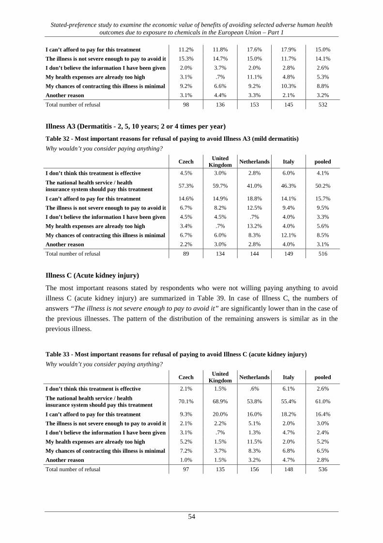
Stated-preference study to examine the economic value of benefits of avoiding selected adverse human health outcomes due to exposure to chemicals in the European Union – Part 1
54
I can’t afford to pay for this treatment 11.2% 11.8% 17.6% 17.9% 15.0% The illness is not severe enough to pay to avoid it 15.3% 14.7% 15.0% 11.7% 14.1% I don’t believe the information I have been given 2.0% 3.7% 2.0% 2.8% 2.6% My health expenses are already too high 3.1% .7% 11.1% 4.8% 5.3% My chances of contracting this illness is minimal 9.2% 6.6% 9.2% 10.3% 8.8% Another reason 3.1% 4.4% 3.3% 2.1% 3.2% Total number of refusal 98 136 153 145 532
Illness A3 (Dermatitis - 2, 5, 10 years; 2 or 4 times per year)
Table 32 - Most important reasons for refusal of paying to avoid Illness A3 (mild dermatitis) Why wouldn’t you consider paying anything?
Czech United Kingdom Netherlands Italy pooled
I don’t think this treatment is effective 4.5% 3.0% 2.8% 6.0% 4.1%
The national health service / health insurance system should pay this treatment 57.3% 59.7% 41.0% 46.3% 50.2%
I can’t afford to pay for this treatment 14.6% 14.9% 18.8% 14.1% 15.7% The illness is not severe enough to pay to avoid it 6.7% 8.2% 12.5% 9.4% 9.5% I don’t believe the information I have been given 4.5% 4.5% .7% 4.0% 3.3% My health expenses are already too high 3.4% .7% 13.2% 4.0% 5.6% My chances of contracting this illness is minimal 6.7% 6.0% 8.3% 12.1% 8.5% Another reason 2.2% 3.0% 2.8% 4.0% 3.1% Total number of refusal 89 134 144 149 516
Illness C (Acute kidney injury)
The most important reasons stated by respondents who were not willing paying anything to avoid illness C (acute kidney injury) are summarized in Table 39. In case of Illness C, the numbers of answers “The illness is not severe enough to pay to avoid it” are significantly lower than in the case of the previous illnesses. The pattern of the distribution of the remaining answers is similar as in the previous illness.
Table 33 - Most important reasons for refusal of paying to avoid Illness C (acute kidney injury) Why wouldn’t you consider paying anything?
Czech United Kingdom Netherlands Italy pooled
I don’t think this treatment is effective 2.1% 1.5% .6% 6.1% 2.6%
The national health service / health insurance system should pay this treatment 70.1% 68.9% 53.8% 55.4% 61.0%
I can’t afford to pay for this treatment 9.3% 20.0% 16.0% 18.2% 16.4% The illness is not severe enough to pay to avoid it 2.1% 2.2% 5.1% 2.0% 3.0% I don’t believe the information I have been given 3.1% .7% 1.3% 4.7% 2.4% My health expenses are already too high 5.2% 1.5% 11.5% 2.0% 5.2% My chances of contracting this illness is minimal 7.2% 3.7% 8.3% 6.8% 6.5% Another reason 1.0% 1.5% 3.2% 4.7% 2.8% Total number of refusal 97 135 156 148 536

Stated-preference study to examine the economic value of benefits of avoiding selected adverse human health outcomes due to exposure to chemicals in the European Union – Part 1
55
True zeros were included into the WTP estimation, while protesters were excluded. Removal of protest responses is done routinely in contingent valuation samples because it is assumed that they are not indicative of respondents’ ‘true’ values.17
Identification of outliers 6.2.
Although some of large amounts stated by respondents may accurately represent actual WTP, other large amounts clearly overstate actual WTP. One frequently used test of reasonableness is to compare the WTP amount with the respondent’s income, but the screen percentage is essentially arbitrary. An alternative favoured for some time was built upon the theory of robust statistics in using trimmed distributions (Mitchell & Carson, 1989, p. 226). A serious drawback of this and similar approaches is that model estimates may be affected by which observations are trimmed from the distribution, as well as the problems associated with trimming asymmetric distributions, including choice of α.18
Smith and Desvousges (1986) use a statistical criterion for identifying observations that exert an undue influence on a regression equation for WTP.19 Their diagnostic is based on estimates of parameter for income using linear-in-parameters model. Those observations then are removed as potential outliers. Even this approach is arbitrary in that it sets a threshold on change in estimated income parameter exerted by outlying observation.
Bearing in mind the potential influence of outlying observations on estimated measures of central tendency on the one hand and arbitrariness brought in by choice of threshold of respective truncation procedure on the other hand, we provide WTP estimates based on two truncation strategies in the remainder of this report:
• the first one (denoted “truncation strategy I”) reports in full the estimates using the dataset censored for (1) observations that are not internally consistent, i.e. respondents stated higher WTP for avoiding illness A than for illness C and at the same time ranked illness C as worse than illness A on visual analogue scales and (2) WTPlower bound amounts in excess of respondent’s income (the thresholds were set at 1, 2 and 3 times monthly income for illness A, illnesses A1&A2, and illnesses A3&C, respectively). The respective numbers of excluded respondents are given in the following table.
• the second truncation strategy (denoted “truncation strategy II”) is based on the regression diagnostics approach as used by Smith and Desvousges (op. cit.); given our substantially
17 Such censoring of protest responses has stirred a definitional controversy – one view is that the definition of protest responses and the rules for censoring them are dependent on whether the practitioner conceives of the contingent valuation survey as a market or as a referendum. The other view is that protest responses and their meaning may vary according to the type of good being valued, the elicitation format, and the interaction between these elements and external factors. See e.g. Jorgensen et al. (1999). 18 Levy et al. (1995) suggests that α-Windsizored mean in positive part of two-part model might be preferable to the α-trimmed mean when used on asymmetric distributions because it is less vulnerable to the bias which is due to the asymmetry in the underlying distribution i.e. reflecting the fact that the positive values of their sample are more symmetrically distributed than the overall sample). 19 This method was originally devised by Belsley, Kuh, and Welsch (1980). In essence, it measures the change in estimated coefficient (of income) as a result of deleting a single observation from the dataset. These n-1 coefficients are normalized by the estimated parameter from the full sample and ranked by the absolute magnitude of the percentage change (i.e. from full sample parameter).

Stated-preference study to examine the economic value of benefits of avoiding selected adverse human health outcomes due to exposure to chemicals in the European Union – Part 1
56
larger samples we use a 0.5 per cent change (in absolute terms) in the estimated parameter for income as the threshold for identifying influential observations that are excluded from the WTP estimation. what translates to elimination of 3 to 5% of total sample. We report WTP estimates based on the dataset truncated by this approach only for pooled data.
Table 34 – Respondents excluded as outliers
truncation strategy I
truncation strategy II internally inconsistent income threshold
illness A 124 59 151 illness A1 128 36 112 illness A2 128 51 124 illness A3 128 37 77 illness C 194 60 161
Apart from protesters and outliers we also excluded 38, 41, 34, 37, and 35 respondents from interval regressions on WTP for a avoiding illnesses A, A1, A2, A3 and C because their lower bound WTP exceeded upper bound WTP.20
Non-parametric WTP estimates 6.3. a) truncation strategy I
Estimated mean and median WTP values from non-parametric models are reported in the following table for pooled data and individual countries. WTP values for avoiding illnesses A1, A2 and A3 are further differentiated by frequency and years of duration and displayed in the following graphs. All estimates were converted to EUR2012 by use of harmonized indices of consumer prices (HICP) and purchasing power parity (PPP) exchange rate.
Survivor curves were estimated separately by respondents’ countries. In common with prevailing evidence from stated preference studies median values are lower than mean because the WTP distribution is right-skewed and influence of this skewness is reduced with the latter measure. The mean and median WTP values are almost always the highest in the Italian sample over all illnesses; mean values are the lowest in the Dutch sample. Czech and UK samples are very similar in mean values for illnesses A, A1 and A2, but UK sample values the rest of illnesses higher.
The mean and median WTP values display only modest differences between illnesses A1, A2 and A3 according to their frequency and duration, although by no means not proportionally. We devote more attention to this in discussion section.
20 When inspecting the dataset we found that majority of these respondents used iPhone or iPad for filling in the questionnaire. Unfortunately, the programme code was not optimized for this option and did not record the data from two-way payment ladder properly.

Stated-preference study to examine the economic value of benefits of avoiding selected adverse human health outcomes due to exposure to chemicals in the European Union – Part 1
57
Figure 15 – Nonparametric estimates of mean and median WTP for avoidance of individual illnesses
Illnesses A and C
Illness A1 (frequency of symptoms 2x or 4x per year)
Illness A2 (occurrence of symptoms once a year over 2, 5 or 10 years)
Illness A3 (occurrence of symptoms 2x or 4x per year over 2, 5 or 10 years)
0
100
200
300
400
500
600
700
illness A illness C
mean WTP (EUR)
cz
en
it
nl
pooled
0
100
200
300
400
500
600
700
illness A illness C
median WTP (EUR)
cz
en
it
nl
pooled
0
100
200
300
400
500
600
700
2x/yr. 4x/yr.
mean WTP (EUR)
cz
en
it
nl
pooled
0
100
200
300
400
500
600
700
2x/yr. 4x/yr.
median WTP (EUR)
cz
en
it
nl
pooled
0
100
200
300
400
500
600
700
2yrs 5yrs 10yrs
mean WTP (EUR)
cz
en
it
nl
pooled
0
100
200
300
400
500
600
700
2yrs 5yrs 10yrs
median WTP (EUR)
cz
en
it
nl
pooled
0
100
200
300
400
500
600
700
2x/yr. 4x/yr. 2x/yr. 4x/yr. 2x/yr. 4x/yr.
2yrs 5yrs 10yrs
mean WTP (EUR)
cz
en
it
nl
pooled
0
100
200
300
400
500
600
700
2x/yr. 4x/yr. 2x/yr. 4x/yr. 2x/yr. 4x/yr.
2yrs 5yrs 10yrs
median WTP (EUR)
cz
en
it
nl
pooled

Stated-preference study to examine the economic value of benefits of avoiding selected adverse human health outcomes due to exposure to chemicals in the European Union – Part 1
58
Table 35 - WTP for avoiding illnesses (truncation strategy I, non-parametric estimates, in “generic” euro/case)
illness A illness A1 illness A2 illness A3 illness C
frequency 2 4 2 4 length 2 5 10 2 5 10 2 5 10
Czech N 797 391 416 275 257 267 146 130 125 156 142 133 819 mean 203.2 253.1 285.6 266.1 306.0 314.5 241.7 374.6 432.2 283.1 326.3 533.5 395.9 median 132 204 204 156 252 240 156 252 348 180 240 396 312
UK N 862 431 439 297 300 263 146 141 155 137 158 149 888 mean 202.9 255.9 307.6 310.7 334.3 312.7 261.9 379.4 549.7 282.2 355.2 530.9 554.6 median 106 159 170 148 201 212 212 212 318 180 276 276 339
Italian N 866 440 439 301 273 286 158 149 161 136 142 148 889 mean 259.3 334.8 361.2 316.6 399.7 350.6 300.2 462.8 389.9 399.2 430.0 683.3 623.4 median 216 245 255 245 265 255 255 314 255 245 294 392 363
Dutch N 570 286 301 198 192 179 111 99 99 103 89 106 584 mean 190.6 245.5 279.6 253.2 264.6 269.3 208.6 189.3 293.9 274.5 307.2 507.9 375.4 median 135 189 180 135 198 180 162 144 171 198 216 315 225
pooled N 3095 1548 1595 1071 1022 995 561 519 540 532 531 536 3180 mean 220.9 278.8 319.6 298.3 341.7 328.6 261.5 377.7 432.1 322.5 369.9 593.5 511.1 median 148 212 225 189 245 252 196 265 276 212 265 315 315

Stated-preference study to examine the economic value of benefits of avoiding selected adverse human health outcomes due to exposure to chemicals in the European Union – Part 1
59
b) truncation strategy II
Non-parametric pooled mean and median WTP values estimated from dataset treated by truncation strategy II are reported in Table 36.
Table 36 - WTP for avoiding illnesses (truncation strategy II, non-parametric estimates, in euro/case)
frequency (per year) length (yrs.) N mean median
illness A 3087 216.0 156
illness A1 2 1555 269.5 212 4 1598 286.4 225
illness A2 2 1047 269.7 189
5 991 283.5 245
10 973 319.0 252
illness A3
2 2 550 239.6 192 5 501 317.3 270
10 535 364.6 276
4 2 519 277.6 212 5 524 354.0 265
10 524 456.6 315
illness C 3068 453.9 314
In short, estimated mean WTP values from truncation strategy II dataset are lower compared to those from truncation strategy I. In contrast, median WTP values remain almost unchanged. Effectively, this suggests that a relatively small group of outliers have a substantial impact on central tendency measures in this right-skewed distribution.21 We illustrate this effect in parametric estimates section in more detail.
Figure 16 - Nonparametric estimates of mean and median WTP (truncation strategy II, pooled)
Note: legend for x-axis – the first line refers to frequency of illness episodes (over a year), the second line refers to length of illness (years)
21 Note however that regression diagnostics trimmed observations from all over the distribution (in contrast to censoring by income).
0
100
200
300
400
500
600
700
(1x/yr) 2x/yr. 4x/yr. (1x/yr) 2x/yr. 4x/yr. (1x/yr) 2x/yr. 4x/yr. (1x/yr) 2x/yr. 4x/yr.
(1yr) 2yrs 5yrs 10yrs
mean WTP (EUR)
illness A illness A1 illness A2 illness A3 illness C
0
100
200
300
400
500
600
700
(1x/yr) 2x/yr. 4x/yr. (1x/yr) 2x/yr. 4x/yr. (1x/yr) 2x/yr. 4x/yr. (1x/yr) 2x/yr. 4x/yr.
(1yr) 2yrs 5yrs 10yrs
median WTP (EUR)
illness A illness A1 illness A2 illness A3 illness C

Stated-preference study to examine the economic value of benefits of avoiding selected adverse human health outcomes due to exposure to chemicals in the European Union – Part 1
60
Parametric WTP estimates 6.4.
We estimate WTP parametrically using the WTP intervals between this amount and the amount that respondent reported as the amount he would most likely not pay (cf. Section 4.1.2). We tested several model specifications to find that lognormal distribution fits our data in slightly better than Weibull with truncation strategy I dataset, while Weibull distribution fits better the data in 2 out of 6 models of WTP on truncation strategy II dataset.
a) truncation strategy I
The following graphs display mean values for individual illnesses, including estimates for illnesses A1-A3 according to their frequency and duration; detailed tables (also for lower bound WTP estimates based on WTPlb) are reported in the Appendix.
Figure 17 – Parametric estimates of mean and median WTP for avoidance of individual illnesses
Illnesses A and C
Illness A1 (frequency of symptoms 2x or 4x per year)
0
100
200
300
400
500
600
700
illness A illness C
mean WTP (EUR)
cz
en
it
nl
pooled
0
100
200
300
400
500
600
700
illness A illness C
median WTP (EUR)
cz
en
it
nl
pooled
0
100
200
300
400
500
600
700
2x/yr. 4x/yr.
mean WTP (EUR)
cz
en
it
nl
pooled
0
100
200
300
400
500
600
700
2x/yr. 4x/yr.
median WTP (EUR)
cz
en
it
nl
pooled

Stated-preference study to examine the economic value of benefits of avoiding selected adverse human health outcomes due to exposure to chemicals in the European Union – Part 1
61
Illness A2 (occurrence of symptoms once a year over 2, 5 or 10 years)
Illness A3 (occurrence of symptoms 2x or 4x per year over 2, 5 or 10 years)
A careful inspection of estimated mean WTP values reveals a paradoxical situation – WTP for avoiding illness A2 lasting once a year over 2 years that is valued higher than illness A3 lasting twice a year over 2 years in pooled data as well as in the Czech, Italian and Dutch subsamples (in Dutch subsample also illness A1 (2x over a year) is valued higher than illness A3 lasting twice a year over 2 years) – what seems to violate the scope test. In fact only 1/18 of the total sample answered to this particular combination and in this particular subsample, illness A3 lasting twice a year over 2 years is valued more than illness A2 lasting once a year over 2 years in pooled data and individual countries’ subsamples (i.e. WTP for avoiding illness A3 is EUR 290 while WTP for avoiding illness A2 is EUR 276 based on pooled data). We explore and test scope sensitivity in detail in Section 9.2.
b) truncation strategy II
The following figure shows parametric estimates of WTP from both lognormal and Weibull models using truncation strategy II dataset. The WTP estimates from both models are very close and the estimates from Weibull models are consistently lower compared to those from lognormal in a range between 0.1% and 12.5%. We observe that avoiding illness A2 lasting once a year over 2 years that is valued higher than illness A3 lasting twice a year over 2 years and that in general the sensitivity to scope is relatively low.
0
100
200
300
400
500
600
700
2yrs 5yrs 10yrs
mean WTP (EUR)
cz
en
it
nl
pooled
0
100
200
300
400
500
600
700
2yrs 5yrs 10yrs
median WTP (EUR)
cz
en
it
nl
pooled
0
100
200
300
400
500
600
700
2x/yr. 4x/yr. 2x/yr. 4x/yr. 2x/yr. 4x/yr.
2yrs 5yrs 10yrs
mean WTP (EUR)
cz
en
it
nl
pooled
0
100
200
300
400
500
600
700
2x/yr. 4x/yr. 2x/yr. 4x/yr. 2x/yr. 4x/yr.
2yrs 5yrs 10yrs
median WTP (EUR)
cz
en
it
nl
pooled

Stated-preference study to examine the economic value of benefits of avoiding selected adverse human health outcomes due to exposure to chemicals in the European Union – Part 1
62
Figure 18 - Parametric estimates of mean WTP (truncation strategy II, pooled)
Note: legend for x-axis – the first line refers to frequency of illness episodes (over a year), the second line refers to length of illness (years)
6.4.1. Validity test
We report two models (both based on a truncation strategy I dataset) – simple and full (survey countries in simple model and additional variables in full model) – for each of five health endpoints differing in number of explanatory variables. We apply a two-part model consisting of a probit model for non-zero WTP in the contingent valuation and interval regression with log-normal density for positive (random) WTP values. Statistical significance of variables in the models is reported using the standard 0.1%, 1% and 5% significance levels.
The tables below summarize the explanatory variables used in the regression models for WTP to avoid each of the health endpoints valued. Income (the income variable used was the country specific decile of household income) is a positive and significant variable in both parts of all the models.
Table 37 - Definition and descriptive statistics of explanatory variables
Description Min Max Mean Std. dev. Czech Republic 1 if respondent is from the Czech Republic 0 1 0.25 0.43 United Kingdom 1 if respondent is from the UK 0 1 0.28 0.45 Italy 1 if respondent is from Italy 0 1 0.19 0.39 Netherlands 1 if respondent is from the Netherlands 0 1 0.28 0.45 Frequency of symptoms - A1 Frequency of symptoms in Illness A1 (2 or 4) 2 4 3.01 1.00 Length of the illness - A2 Length of the illness A2 (2, 5, 10) 2 10 5.62 3.30 Frequency of symptoms - A3 Frequency of symptoms in illness A3 (2 or 4) 2 4 2.99 1.00 Length of the illness - A3 Length of the illness A3 (2, 5, 10) 2 10 5.69 3.31 Household income Household income (income deciles) 1 10 4.84 2.65 Age Age of the respondent 17 66 41.77 13.23 Lower_secondary 1 if respondent attained lower secondary education 0 1 0.18 0.39 Upper_secondary 1 if respondent attained upper secondary education 0 1 0.57 0.50 Tertiary 1 if respondent attained tertiary education 0 1 0.22 0.41 Gender (female) 1 if respondent is female 0 1 0.50 0.50 CurrHealth Current health state (VAS 0-100) 0 100 60.73 19.90 HealthImpact Perceived health impact (change in VAS rating) 0 90 17.53 19.66 Employ 1 if respondent is employed 30 hours or more 0 1 0.45 0.50
0
100
200
300
400
500
600
700
(1x/yr) 2x/yr. 4x/yr. (1x/yr) 2x/yr. 4x/yr. (1x/yr) 2x/yr. 4x/yr. (1x/yr) 2x/yr. 4x/yr.
(1yr) 2yrs 5yrs 10yrs
mean WTP (EUR), lognormalillness A illness A1 illness A2 illness A3 illness C
0
100
200
300
400
500
600
700
(1x/yr) 2x/yr. 4x/yr. (1x/yr) 2x/yr. 4x/yr. (1x/yr) 2x/yr. 4x/yr. (1x/yr) 2x/yr. 4x/yr.
(1yr) 2yrs 5yrs 10yrs
mean WTP (EUR), Weibullillness A illness A1 illness A2 illness A3 illness C

Stated-preference study to examine the economic value of benefits of avoiding selected adverse human health outcomes due to exposure to chemicals in the European Union – Part 1
63
Description Min Max Mean Std. dev.
Married 1 if respondent is married or in registered partnership 0 1 0.54 0.50
Child Number of children in the household 1 6 1.66 0.92
The results in both parts of the model and for each endpoint show that respondent’s country variables (with Czech sample taken as status-quo) have significant effects. Respondents from the Netherlands have a lower probability to express non-zero WTP in the contingent valuation and also tendency to express lower WTP. The effect of the country on the participation is not significant for UK and Italy, but Italian respondents tend to state higher WTP for all endpoints. The effect of the UK variable on stated WTP is negative for all endpoints and statistically significant for illnesses A and A1 (acute dermatitis with a single occurrence or with 2 or 4 episodes over one year). Age seems to be a negative but statistically insignificant predictor of expressing non-zero WTP but a positive and statistically significant predictor of stated (positive) WTP across all endpoints.
Higher education (upper secondary and tertiary) is a positive and statistically significant predictor for expressing non-zero WTP in the contingent valuation for all health endpoints with the exception of illness A2 (dermatitis lasting 2, 5 or 10 years). Higher education is also a positive predictor of stated (positive) WTP - the upper secondary education is however statistically significant only for Illness A3 (dermatitis episodes 2x or 4x per year over 2, 5 or 10 years) and C (acute kidney injury); the tertiary education is significant only for Illness A3 and C. Gender (female) has a negative effect on the participation in the contingent valuation, but not statistically significant. Female respondent also tend to state lower WTP but the difference is statistically significant only for illness A. Subjective evaluation of own health (on a VAS scale) is significant predictor of expressing non-zero WTP for all the endpoints. In contrast, subjective rating of perceived health impact of either illness A22 or illness C is a significant predictor of stated (positive) WTP for all the endpoints.
A three other socio-demographic predictors were tested the model: employment 30 hours a week or more (a binary variable), marital status and number of children below 18 years in the household. None of these variables has a statistically significant effect on the participation in the contingent valuation or stated WTP.
Finally, the effect of two attributes of skin sensitisation (acute dermatitis) endpoints was investigated, i.e. frequency of the symptoms (per year) and how many years the symptoms occur. Both the frequency and length have a positive and statistically significant effect on stated WTP to avoid the respective illness, but not on the probability of non-zero WTP. The size of these coefficients are however very small, meaning that the marginal change in number of sensitization episodes (irrespective whether in a year or over several years) brings only modest increase in total WTP. We explore the effect of frequency and length further in a joint model of WTP for avoidance of illnesses A through A3 in Section 6.4.2.
22 Note that health rating using VAS was elicited for health states A and C. Since illnesses A1, A2 and A3 are using the profile of illness A, we use health rating of illness A as an explanatory variable in regressions on WTP for avoiding these three related health states.

Stated-preference study to examine the economic value of benefits of avoiding selected adverse human health outcomes due to exposure to chemicals in the European Union – Part 1
64
Table 38 - Parametric model of zero WTP (part 1 model) and positive WTP (part 2 model) for avoiding illness A (acute dermatitis) full model simple model full model simple model
part 1 model (probit) Coef. Std.Err. Coef. Std.Err. Constant 0.881 ** 0.290 1.630 *** 0.074 United Kingdom -0.376 *** 0.108 -0.235 * 0.097 Italy -0.071 0.110 -0.067 0.101 Netherlands -0.628 *** 0.107 -0.566 *** 0.099 Household income 0.048 ** 0.015 Age -0.003 0.003 Lower_secondary 0.185 0.200 Upper_secondary 0.459 * 0.196 Tertiary 0.622 ** 0.211 Gender (female) -0.134 . 0.072 CurrHealth 0.005 * 0.002 HealthImpact 0.002 0.002 Employ 0.086 0.076 Married -0.062 0.085 Child -0.021 0.038
part 2 model (lognormal – positive, lower bound WTP) (lognormal – positive, interval WTP data) Coef. Std.Err. Coef. Std.Err. Coef. Std.Err. Coef. Std.Err. Constant 3.619 *** 0.194 4.438 *** 0.041 4.303 *** 0.186 4.981 *** 0.039 United Kingdom -0.142 * 0.059 -0.107 . 0.057 -0.183 ** 0.057 -0.149 ** 0.054 Italy 0.320 *** 0.058 0.327 *** 0.057 0.286 *** 0.056 0.285 *** 0.054 Netherlands 0.065 0.066 0.068 0.065 -0.001 0.062 -0.010 0.061 Household income 0.056 *** 0.009 0.057 *** 0.008 Age 0.012 *** 0.002 0.009 *** 0.002 Lower_secondary 0.109 0.141 0.130 0.134 Upper_secondary 0.221 0.137 0.191 0.130 Tertiary 0.130 0.142 0.147 0.135 Gender (female) -0.190 *** 0.043 -0.119 ** 0.041 CurrHealth -0.001 0.001 -0.002 0.001 HealthImpact 0.005 *** 0.001 0.005 *** 0.001 Employ 0.021 0.044 0.013 0.042 Married 0.002 0.051 0.029 0.049 Child 0.002 0.023 -0.012 0.022 s.d. 1.087 *** 0.014 1.120 *** 0.015 -0.028 0.015 0.002 0.014 Log-Likelihood: -17910 -18032 - 4780.3 -4890.6
Signif. codes: ***0.001, **0.01, * 0.05.

Stated-preference study to examine the economic value of benefits of avoiding selected adverse human health outcomes due to exposure to chemicals in the European Union – Part 1
65
Table 39 - Parametric model of zero WTP (part 1 model) and positive WTP (part 2 model) for avoiding illness A1 (dermatitis: 2x or 4x) full model simple model full model simple model
part 1 model (probit) Coef. Std.Err. Coef. Std.Err. Constant 1.107 ** 0.352 1.846 *** 0.144 United Kingdom -0.446 *** 0.130 -0.267 * 0.116 Italy -0.330 ** 0.127 -0.293 * 0.115 Netherlands -0.789 *** 0.126 -0.677 *** 0.114 Frequency of symptoms - A1 0.037 0.039 0.026 0.037 Household income 0.042 * 0.017 Age -0.005 0.003 Lower_secondary -0.046 0.239 Upper_secondary 0.269 0.236 Tertiary 0.524 * 0.255 Gender (female) -0.104 0.081 CurrHealth 0.010 *** 0.002 HealthImpact 0.001 0.002 Employ 0.032 0.086 Married 0.004 0.095 Child -0.062 0.041
part 2 model (lognormal – positive, lower bound WTP) (lognormal – positive, interval WTP data) Coef. Std.Err. Coef. Std.Err. Coef. Std.Err. Coef. Std.Err. Constant 3.620 *** 0.187 4.660 *** 0.071 4.231 *** 0.179 5.129 *** 0.067 United Kingdom -0.140 * 0.056 -0.085 0.054 -0.159 ** 0.053 -0.118 * 0.051 Italy 0.276 *** 0.055 0.264 *** 0.054 0.260 *** 0.052 0.239 *** 0.051 Netherlands 0.035 0.061 0.040 0.061 -0.015 0.058 -0.026 0.057 Frequency of symptoms - A1 0.049 * 0.019 0.050 * 0.020 0.045 * 0.018 0.046 * 0.019 Household income 0.065 *** 0.008 0.062 *** 0.008 Age 0.012 *** 0.002 0.010 *** 0.002 Lower_secondary 0.071 0.128 0.067 0.123 Upper_secondary 0.214 . 0.124 0.161 0.119 Tertiary 0.206 0.129 0.173 0.123 Gender (female) -0.108 ** 0.040 -0.050 0.038 CurrHealth 0.001 0.001 0.000 0.001 HealthImpact 0.003 ** 0.001 0.003 ** 0.001 Employ 0.037 0.041 0.035 0.039 Married -0.045 0.048 -0.039 0.045 Child -0.006 0.022 -0.011 0.021 s.d. 1.051 *** 0.014 1.083 *** 0.014 -0.053 0.014 -0.026 0.014 Log-Likelihood: -19689 -19821 -5485.3 -5563

Stated-preference study to examine the economic value of benefits of avoiding selected adverse human health outcomes due to exposure to chemicals in the European Union – Part 1
66
Table 40 - Parametric model of zero WTP (part 1 model) and positive WTP (part 2 model) for avoiding illness A2 (dermatitis: once a year over 2, 5, or 10 years) full model simple model full model simple model
part 1 model (probit) Coef. Std. Err. Coef. Std. Err. Constant 0.763 * 0.328 1.744 *** 0.104 United Kingdom -0.179 0.126 -0.047 0.113 Italy -0.228 . 0.119 -0.209 . 0.108 Netherlands -0.656 *** 0.119 -0.579 *** 0.108 Length of the illness - A2 0.011 0.012 0.010 0.011 Household income 0.053 ** 0.017 Age -0.002 0.003 Lower_secondary 0.072 0.226 Upper_secondary 0.306 0.222 Tertiary 0.555 * 0.241 Gender (female) -0.048 0.081 CurrHealth 0.009 *** 0.002 HealthImpact 0.001 0.002 Employ 0.035 0.085 Married -0.055 0.095 Child -0.049 0.041
part 2 model (lognormal – positive, lower bound WTP) (lognormal – positive, interval WTP data) Coef. Std. Err. Coef. Std. Err. Coef. Std. Err. Coef. Std. Err. Constant 3.720 *** 0.192 4.683 *** 0.054 4.260 *** 0.181 5.177 *** 0.051 United Kingdom -0.086 0.058 -0.048 0.056 -0.118 * 0.055 -0.085 0.053 Italy 0.260 *** 0.058 0.252 *** 0.056 0.218 *** 0.055 0.201 *** 0.053 Netherlands 0.012 0.065 0.009 0.064 -0.068 0.061 -0.082 0.060 Length of the illness - A2 0.030 *** 0.006 0.031 *** 0.006 0.025 *** 0.006 0.026 *** 0.006 Household income 0.066 *** 0.009 0.065 *** 0.008 Age 0.012 *** 0.002 0.011 *** 0.002 Lower_secondary 0.016 0.136 0.051 0.129 Upper_secondary 0.144 0.132 0.124 0.124 Tertiary 0.078 0.137 0.109 0.129 Gender (female) -0.108 * 0.042 -0.052 0.040 CurrHealth 0.000 0.001 0.000 0.001 HealthImpact 0.004 *** 0.001 0.004 *** 0.001 Employ 0.041 0.043 0.047 0.041 Married -0.042 0.051 -0.021 0.048 Child -0.007 0.023 -0.017 0.022 s.d. 1.092 *** 0.014 1.125 *** 0.015 -0.012 0.014 0.019 0.014 Log-Likelihood: -19533 -19658 -5580 -5663

Stated-preference study to examine the economic value of benefits of avoiding selected adverse human health outcomes due to exposure to chemicals in the European Union – Part 1
67
Table 41 - Parametric model of zero WTP (part 1 model) and positive WTP (part 2 model) for avoiding illness A3 (dermatitis: 2x or 4x a year over 2, 5, or 10 years) full model simple model full model simple model
part 1 model (probit) Coef. Std. Err. Coef. Std. Err. Constant 0.607 . 0.365 1.816 *** 0.160 United Kingdom -0.313 * 0.141 -0.106 0.122 Italy -0.326 * 0.134 -0.238 * 0.117 Netherlands -0.850 *** 0.132 -0.678 *** 0.115 Frequency of symptoms - A3 0.040 0.041 0.035 0.039 Length of the illness - A3 0.004 0.012 0.001 0.012 Household income 0.071 *** 0.019 Age -0.004 0.004 Lower_secondary 0.147 0.232 Upper_secondary 0.451 * 0.229 Tertiary 0.805 ** 0.256 Gender (female) -0.062 0.087 CurrHealth 0.012 *** 0.003 HealthImpact 0.000 0.002 Employ -0.044 0.092 Married 0.106 0.100 Child -0.111 ** 0.043
part 2 model (lognormal – positive, lower bound WTP) (lognormal – positive, interval WTP data) Coef. Std. Err. Coef. Std. Err. Coef. Std. Err. Coef. Std. Err. Constant 3.487 *** 0.208 4.482 *** 0.084 4.060 *** 0.195 4.971 *** 0.079 United Kingdom -0.031 0.060 0.026 0.057 -0.081 0.056 -0.032 0.054 Italy 0.268 *** 0.059 0.249 *** 0.057 0.225 *** 0.056 0.203 *** 0.054 Netherlands -0.034 0.066 -0.022 0.065 -0.111 0.062 -0.109 0.061 Frequency of symptoms - A3 0.069 *** 0.021 0.074 *** 0.021 0.062 ** 0.019 0.067 *** 0.020 Length of the illness - A3 0.047 *** 0.006 0.048 *** 0.006 0.044 *** 0.006 0.046 *** 0.006 Household income 0.070 *** 0.009 0.066 *** 0.008 Age 0.011 *** 0.002 0.009 *** 0.002 Lower_secondary 0.032 0.140 0.075 0.132 Upper_secondary 0.169 0.136 0.159 0.127 Tertiary 0.189 0.141 0.199 0.132 Gender (female) -0.060 0.043 -0.037 0.041 CurrHealth 0.001 0.001 0.001 0.001 HealthImpact 0.003 * 0.001 0.003 ** 0.001 Employ -0.001 0.044 -0.001 0.042 Married -0.037 0.052 -0.017 0.049 Child -0.016 0.024 -0.022 0.022 s.d. 1.125 *** 0.015 1.153 *** 0.015 0.014 0.014 0.038 ** 0.014 Log-Likelihood: -20126 -20252 -5839 -5907.5

Stated-preference study to examine the economic value of benefits of avoiding selected adverse human health outcomes due to exposure to chemicals in the European Union – Part 1
68
Table 42 - Parametric model of zero WTP (part 1 model) and positive WTP (part 2 model) for avoiding illness C (acute kidney injury) full model simple model full model simple model
part 1 model (probit) Coef. Std. Error Coef. Std. Error Constant 1.130 ** 0.358 2.052 *** 0.102 United Kingdom -0.487 ** 0.153 -0.246 . 0.130 Italy -0.310 * 0.151 -0.259 * 0.130 Netherlands -0.822 *** 0.148 -0.684 *** 0.127 Household income 0.086 *** 0.021 Age -0.009 * 0.004 Lower_secondary 0.118 0.243 Upper_secondary 0.446 . 0.241 Tertiary 0.811 ** 0.274 Gender (female) 0.021 0.094 CurrHealth 0.009 ** 0.003 HealthImpact 0.002 0.002 Employ 0.046 0.101 Married -0.049 0.110 Child -0.055 0.048
part 2 model (lognormal – positive, lower bound WTP) (lognormal – positive, interval WTP data) Coef. Std. Err. Coef. Std. Err. Coef. Std. Error Coef. Std. Error Constant 3.968 *** 0.178 5.166 *** 0.038 4.415 *** 0.167 5.583 *** 0.036 United Kingdom 0.214 *** 0.056 0.312 *** 0.053 0.180 *** 0.052 0.265 *** 0.050 Italy 0.385 *** 0.056 0.404 *** 0.054 0.346 *** 0.052 0.352 *** 0.050 Netherlands 0.068 0.061 0.080 0.061 0.030 0.057 0.027 0.057 Household income 0.071 *** 0.008 0.073 *** 0.008 Age 0.012 *** 0.002 0.010 *** 0.002 Lower_secondary 0.175 0.129 0.209 0.121 Upper_secondary 0.342 ** 0.124 0.322 ** 0.117 Tertiary 0.392 ** 0.129 0.396 ** 0.122 Gender (female) -0.070 . 0.040 -0.057 0.038 CurrHealth 0.000 0.001 0.000 0.001 HealthImpact 0.004 *** 0.001 0.004 *** 0.001 Employ 0.014 0.041 0.014 0.038 Married -0.064 0.048 -0.054 0.045 Child -0.009 0.022 -0.012 0.021 s.d. 1.035 *** 0.013 1.071 *** 0.014 -0.070 0.014 -0.032 * 0.014 Log-Likelihood: -20654 -20812 -5854 -5960.6

Stated-preference study to examine the economic value of benefits of avoiding selected adverse human health outcomes due to exposure to chemicals in the European Union – Part 1
69
6.4.2. Joint estimation of WTP for avoiding illnesses A through A3
The model of WTP for avoidance of illnesses A through A3 (where illness A is a situation when illness occurs once in the next year only) is hence as follows:
𝑊𝑊𝑊 = 𝛼 + 𝛽1𝑙𝑙𝑙𝑙𝑙ℎ + 𝛽2𝑓𝑃𝑙𝑓𝑓𝑙𝑙𝑓𝑦 + 𝛽3(𝑙𝑙𝑙𝑙𝑙ℎ × 𝑓𝑃𝑙𝑓𝑓𝑙𝑙𝑓𝑦)
We report two models outcomes, model 1 with dummies for alternating illness lengths and frequencies (and interactions), and model 2 where length, frequency and their interaction are taken as continuous variables.
Table 43 – Regression models for joint estimation of WTP for avoiding illnesses A through A3
model 1 model 2 Coef. Std. Error Coef. Std. Error constant 3.9880 *** 0.1607 3.8857 *** 0.1612 length of illness 0.0600 *** 0.0027
2y 0.2167 *** 0.0185 5y 0.3854 *** 0.0185 10y 0.4513 *** 0.0187
frequency of illness 0.1193 *** 0.0054 2x/yr 0.2320 *** 0.0159 4x/yr 0.3693 *** 0.0157
frequency∗length -0.0083 *** 0.0012 2_2 -0.1833 *** 0.0319 2_4 -0.1810 *** 0.0324 5_2 -0.1607 *** 0.0329 5_4 -0.1997 *** 0.0321 10_2 -0.1537 *** 0.0325 10_4 -0.2065 *** 0.0322
United Kingdom -0.1456 ** 0.0507 -0.1434 ** 0.0508 Italy 0.1981 *** 0.0502 0.1990 *** 0.0502 Netherlands -0.0826 0.0559 -0.0804 0.0560 Household income 0.0666 *** 0.0071 0.0670 *** 0.0071 Lower_secondary 0.1695 0.1198 0.1696 0.1199 Upper_secondary 0.2423 * 0.1158 0.2438 * 0.1159 Tertiary 0.2542 * 0.1200 0.2550 * 0.1202 Age 0.0091 *** 0.0014 0.0091 *** 0.0014 Gender (female) -0.0865 * 0.0357 -0.0863 * 0.0358 CurrHealth 0.0003 0.0012 0.0003 0.0012 HealthImpact 0.0044 *** 0.0010 0.0044 *** 0.0010 σν 0.8992 *** 0.0129 0.9000 *** 0.0129 σε 0.3769 *** 0.0028 0.3827 *** 0.0029 ρ 0.8506 0.0042 0.8469 0.0042 Log-likelihood -15194.2 -15299.8 Notes: σν is the panel-level and σε is the overall variance component.
The results from model 1 are consistent with our expectations – the coefficients of length and frequency are significant and positive and increase with increase in length or frequency. The coefficient of interaction term is negative meaning that if both length and frequency increase there is

Stated-preference study to examine the economic value of benefits of avoiding selected adverse human health outcomes due to exposure to chemicals in the European Union – Part 1
70
an implicit “discount” for such combination, i.e. suggesting that WTP for more frequent and longer lasting episodes of allergic dermatitis is not a simple sum of WTPs for individual episodes. Other statistically significant variables are household income (higher income has positive effect on WTP), higher education (positive), age (positive), gender (negative for females) and subjective evaluation of decrement in health-related quality of life by suffering from acute mild dermatitis (positive effect, i.e. the worse the decrement is perceived the higher is WTP).
Model 2 confirms these findings – the length and frequency coefficients are positive and the coefficient of their interaction is negative (and substantially smaller). This model is particularly useful for illustrating how the slopes of length and frequency variables interact. Setting episodes frequency as a moderator variable at predefined levels (1x, 2x and 4x/year) we compute the slope for WTP on length. This gives the amount of change in WTP with one unit change in length while holding frequency constant at predefined values (average marginal effects); the values are 0.051, 0.043 and 0.027 for 1, 2 and 4 years, respectively. We compute intercepts for each of these slopes (with length set to zero) and plot the slopes in the following graph. The bottom line is the slope when frequency equals 1, in the middle is the slope when frequency equals 2 and the upper line represent the slope when frequency equals 4. Length of illness (in years) is shown on x axis and logarithm of median WTP on axis y.
Figure 19 – Changes in WTP relative to duration of sensitization episodes
Setting illness length as a moderator variable at predefined levels (1, 2, 5 and 10 years) we compute the slope for WTP on frequency. This gives the amount of change in WTP with one unit change in frequency while holding length constant at predefined values (average marginal effects); the values are 0.111, 0.103, 0.078 and 0.036 for 1, 2, 5 and 10 years, respectively. We compute intercepts for each of these slopes (with frequency set to 1) and plot the slopes in the following graph. The bottom line is the slope when length equals 1, the second is the slope when length equals 2, the third is the slope for length equal to 5 and the upper line represent the slope when length equals 10. Frequency of illness (per year) is shown on x axis and logarithm of median WTP is shown on y axis.

Stated-preference study to examine the economic value of benefits of avoiding selected adverse human health outcomes due to exposure to chemicals in the European Union – Part 1
71
Figure 20 – Changes in WTP relative to frequency of sensitization episodes
6.4.3. Income elasticity of WTP The income elasticity of WTP was estimated using simple double-log (i.e. logarithms of WTP and income) models. We employed two variants – in the first one we estimated the gross impact of income (i.e. income as the only explanatory variable), and controlling also for the significant individual characteristics observed in the WTP validity tests – age, education and sex (and frequency and duration of illness for illnesses A1, A2 and A3) in the second variant. A stylized model used to estimate income-elasticity of WTP is as follows:
𝑙𝑙𝑙(𝑊𝑊𝑊) = 𝛼 + 𝛽 × 𝑙𝑙𝑙(𝑖𝑙𝑓𝑙𝑖𝑙) + 𝛿 × 𝑥𝑖 + 𝜀
where β corresponds to the income-elasticity of WTP, δ is a k x 1 vector of unknown parameters, x is the 1 x k vector of individual characteristics, and ε is the error term. In the second variant we estimated gross impact of income so that income was the only explanatory variable in the model.
The sub-sample used for estimation did not include protesters and true-zero respondents.23 We used WTP as interval and midpoint of household income interval for model estimations – these were run for pooled as well as for individual countries for illnesses A, A1, A2, A3 and C. Both WTP and household income were PPP-corrected. As Table 44 shows, the results were similar using both variants of the model.
Table 44 – Estimated WTP income elasticities
CZ EN IT NL pooled gross impact of income
A 0.31 *** 0.37 *** 0.20 *** 0.11 n.s. 0.25 *** A1 0.34 *** 0.34 *** 0.26 *** 0.13 n.s. 0.27 *** A2 0.38 *** 0.34 *** 0.30 *** 0.16 * 0.29 ***
23 We have excluded true-zero respondents simply because logarithm of zero is not tractable in the above formula.

Stated-preference study to examine the economic value of benefits of avoiding selected adverse human health outcomes due to exposure to chemicals in the European Union – Part 1
72
A3 0.32 *** 0.36 *** 0.28 *** 0.19 * 0.29 *** C 0.37 *** 0.35 *** 0.38 *** 0.19 ** 0.35 ***
partial impact of income A 0.30 *** 0.35 *** 0.10 n.s. 0.10 n.s. 0.24 ***
A1 0.31 *** 0.31 *** 0.18 ** 0.12 n.s. 0.25 *** A2 0.38 *** 0.32 *** 0.21 *** 0.16 * 0.28 *** A3 0.29 *** 0.31 *** 0.20 ** 0.14 n.s. 0.27 *** C 0.34 *** 0.31 *** 0.29 *** 0.17 * 0.30 ***
Signif. codes: ***0.001, **0.01, * 0.05
The relatively low elasticities could potentially be due to the fact that WTP amounts for theses illnesses make up a small proportion of income for most income categories and countries. Thus it may not be surprising that for the less severe illnesses the income elasticity is not significantly different from zero in the Dutch sample (and in Italian sample for partial impact). Interestingly, we observe similar elasticities in the Czech and UK samples, but the patterns are not quite consistent.
Standard gamble with chaining 6.5. In each of the three standard gambles we elicited intervals between the highest accepted and the next (i.e. not accepted) chance of new treatment failure. The following graph shows cumulative distribution functions (using Kaplan-Meier non-parametric estimator) of minimum treatment success preferred by respondents in the three standard gambles. It shows what proportion of respondents (on y axis) accepted at least the chance of success (indicated as percentage on x axis). The minimum treatment success had to be higher than 50% for more than 60% of respondents in all the three gambles. Interestingly, the distribution functions for the first and third standard gambles are very close and the asymptotic Wilcoxon test does not exclude equality (Z=0.466, p-value=0.641), while the statistical distribution of the second standard gamble responses is different (χ2=122.4, p-value<0.001).
Figure 21 – Kaplan-Meier non-parametric estimators of distribution of minimum new treatment success in each standard gamble
0.00
0.25
0.50
0.75
1.00
0 25 50 75 100min. treatment succes
cdf
SG no.
SG1
SG2
SG3

Stated-preference study to examine the economic value of benefits of avoiding selected adverse human health outcomes due to exposure to chemicals in the European Union – Part 1
73
The following table shows the midpoints from intervals between the highest accepted chance of new treatment failure and the next (i.e. not accepted) chance of new treatment failure for the first standard gamble.
Table 45 - Accepted chances of new treatment failure in 1st standard gamble (means of intervals’ mid-points)
Illness A3 variants accepted chance of new treatment failure (i.e. illness B)
frequency (times/yr.) length (yrs.) pooled 2 2 36.8% 2 5 38.7% 2 10 40.3% 4 2 36.6% 4 5 38.5% 4 10 40.1%
The accepted chances of treatment failure differ between illness A3 variants (and seem to differ by length more than by frequency), also asymptotic Wilcoxon k-sample test excludes (although by a narrow margin) the equality of statistical distributions of accepted risk intervals by illness A3 variant (χ2=11.75, p-value=0.038).
Figure 22 – Kaplan-Meier non-parametric estimators of distribution of minimum new treatment success in SG-1 sub-variants
Note: l – length (2, 5 or 10 years) and f - frequency (2x or 4x per year) of illness A3 episodes
The next table shows the midpoints of intervals between highest accepted chance of new treatment failure and the next (i.e. not accepted) chance of new treatment failure for the second and the third standard gambles. We use these midpoints as point of indifference between the two treatments presented, i.e. the product of this indifference midpoint and WTP for avoiding new treatment failure equals to WTP for avoiding conventional treatment outcome.
0.00
0.25
0.50
0.75
1.00
0 25 50 75 100min. treatment success
cdf
SG1 variant
l10f2
l10f4
l2f2
l2f4
l5f2
l5f4

Stated-preference study to examine the economic value of benefits of avoiding selected adverse human health outcomes due to exposure to chemicals in the European Union – Part 1
74
Table 46 – Accepted chances of new treatment failure in 2nd and 3rd standard gamble (means of intervals’ mid-points)
outcome of
conventional treatment
outcome of new treatment
failure Czech English Italian Dutch pooled
SG2 illness C illness D 38.5% 29.9% 31.2% 29.7% 32.4%
SG3 illness B illness D 44.5% 35.3% 35.2% 38.8% 38.2%
The distribution of lowest accepted risk of novel treatment success for all standard gambles (incl. variants in SG1) is shown in the following figure. Whilst it is not surprising that a part of respondents turns out to be very risk averse (corresponding to a peak at 100% treatment success), we also observe a number of respondents with exactly the opposite behaviour, accepting more than 99% risk of treatment failure.24
24 These extremes have been observed also in HEIMTSA valuation study and their plausibility was probed in a focus group interview conducted between pilot and main wave. Indeed, some of the focus group participants inclined to either of these extremes providing meaningful reasons, i.e. arguing that ‘any chance of a cure is worth trying’ or that the health state if treatment fails is so debilitating that the change of failure must be minimal.

Stated-preference study to examine the economic value of benefits of avoiding selected adverse human health outcomes due to exposure to chemicals in the European Union – Part 1
75
Figure 23 – Mean accepted chance of new treatment success
Notes: f – frequency (2x or 4x per year), l – length (for over 2, 5 or 10 years)
Following the approach taken by Bateman et al. (2009) we use mean WTP values from contingent valuation and mean accepted risk trade-offs from standard gambles to derive stepwise WTP for avoiding Illness B (chronic severe dermatitis), and Illness D (chronic kidney disease). The chaining is applied to mean WTP values from non-parametric estimates.
SG 1 [f=2; l=2]
mean accepted chance of
Freq
uenc
y
0 20 40 60 80 100
030
60SG 1 [f=2; l=5]
mean accepted chance o
Freq
uenc
y
0 20 40 60 80 100
040
80
SG 1 [f=2; l=10]
mean accepted chance of
Freq
uenc
y
0 20 40 60 80 100
030
60
SG 1 [f=4; l=2]
mean accepted chance o
Freq
uenc
y0 20 40 60 80 100
030
60
SG 1 [f=4; l=5]
mean accepted chance of
Freq
uenc
y
0 20 40 60 80 100
030
60
SG 1 [f=4; l=10]
mean accepted chance o
Freq
uenc
y
0 20 40 60 80 100
040
80
SG 2
mean accepted chance of n
Freq
uenc
y
0 20 40 60 80 100
010
030
0
SG 3
mean accepted chance of n
Freq
uenc
y
0 20 40 60 80 100
010
030
0
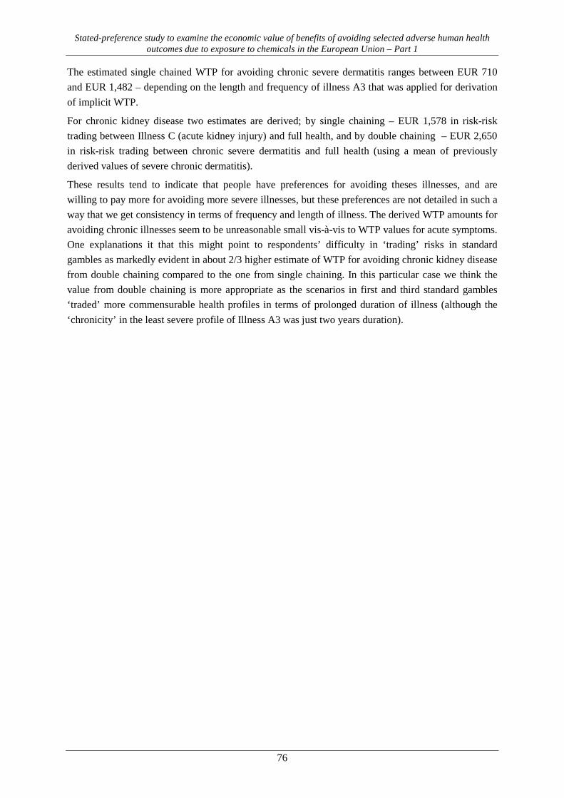
Stated-preference study to examine the economic value of benefits of avoiding selected adverse human health outcomes due to exposure to chemicals in the European Union – Part 1
76
The estimated single chained WTP for avoiding chronic severe dermatitis ranges between EUR 710 and EUR 1,482 – depending on the length and frequency of illness A3 that was applied for derivation of implicit WTP.
For chronic kidney disease two estimates are derived; by single chaining – EUR 1,578 in risk-risk trading between Illness C (acute kidney injury) and full health, and by double chaining – EUR 2,650 in risk-risk trading between chronic severe dermatitis and full health (using a mean of previously derived values of severe chronic dermatitis).
These results tend to indicate that people have preferences for avoiding theses illnesses, and are willing to pay more for avoiding more severe illnesses, but these preferences are not detailed in such a way that we get consistency in terms of frequency and length of illness. The derived WTP amounts for avoiding chronic illnesses seem to be unreasonable small vis-à-vis to WTP values for acute symptoms. One explanations it that this might point to respondents’ difficulty in ‘trading’ risks in standard gambles as markedly evident in about 2/3 higher estimate of WTP for avoiding chronic kidney disease from double chaining compared to the one from single chaining. In this particular case we think the value from double chaining is more appropriate as the scenarios in first and third standard gambles ‘traded’ more commensurable health profiles in terms of prolonged duration of illness (although the ‘chronicity’ in the least severe profile of Illness A3 was just two years duration).

Stated-preference study to examine the economic value of benefits of avoiding selected adverse human health outcomes due to exposure to chemicals in the European Union – Part 1
77
Table 47 - Implicit WTP for avoiding health endpoints (in EUR per case, PPP-corrected)
Conventional treatment Novel treatment Point of
indifference
WTP for avoiding outcome of
conventional treatment
Implicit WTP from standard gambles
freq.
(times/yr.) length (yrs.)
N success failure B: Chronic derm. - severe D: Chronic kidney disease
non-parametric WTP
A3: mild dermatitis
2 2 616 full health B: Chronic derm. - severe 36.8% 261 710
2 5 599 full health B: Chronic derm. - severe 38.7% 377 975
2 10 616 full health B: Chronic derm. - severe 40.3% 432 1071
4 2 594 full health B: Chronic derm. - severe 36.6% 322 881
4 5 601 full health B: Chronic derm. - severe 38.5% 370 960
4 10 608 full health B: Chronic derm. - severe 40.1% 594 1482
C: Acute kidney injury 3634 full health D: chronic kidney disease 32.4% 511 1578 B: Chronic dermatitis - severe
3634 full health D: chronic kidney disease 38.8% 2650
parametric WTP
A3: mild dermatitis
2 2 511 full health B: Chronic derm. - severe 36.8% 304 827
2 5 463 full health B: Chronic derm. - severe 38.7% 352 911
2 10 465 full health B: Chronic derm. - severe 40.3% 441 1093
4 2 492 full health B: Chronic derm. - severe 36.6% 348 952
4 5 500 full health B: Chronic derm. - severe 38.5% 396 1028
4 10 462 full health B: Chronic derm. - severe 40.1% 505 1260
C: Acute kidney injury 2926 full health D: chronic kidney disease 31.5% 492 1519 B: Chronic dermatitis - severe
2926 full health D: chronic kidney disease 38.0% 2646

Stated-preference study to examine the economic value of benefits of avoiding selected adverse human health outcomes due to exposure to chemicals in the European Union – Part 1
78
7. Health rating and QALY
In this chapter we report our findings from health rating and derive QALY weight and QALY losses for illnesses A, B, C and D. Foremost, we see that the option to revise health rankings after all the ratings were done has led a lot of respondents to adjust their ratings. Consequently, the differences between original and revised ratings are statistically significant in current health ratings, and also in ratings of illness A in Italian and Dutch sub-samples, while revisions of ratings of remaining health outcomes are not statistically significant (at the conventional 0.05 level).
As the tables reported in chapter 5.4.2 above suggest, respondents’ health state ratings are significantly different among country samples. Also, respondents who were diagnosed with eczema, allergy, acute kidney injury or chronic kidney disease report significantly lower rating of their current health state, but do not report statistically different ratings of any of the four health outcomes. A similar pattern also emerges when a family member of close friend is diagnosed eczema, allergy, acute of chronic kidney disease, i.e. respondents report significantly lower rating of their current health state, but there’s no difference in ratings of the four health outcomes.
Further, the current health ranking is negatively associated with respondents’ age and positively associated with household income. Interestingly the association with age is statistically significant also in ranking of illness A (p<0.001) and illness D (p<0.05), and association with household income is significant in ranking of all illnesses but illness D. We also find that males tend to rate illness D significantly higher than females (p<0.001).
To allow for comparison between WTP and VAS ratings we have taken the following approach. The CV scenario suggested that the respondent’s general health in the coming year would be exactly the same as in the previous with exeception of an episode of illness A. Hence we elicited WTP for change in utility with respect to health currently experienced. In contrast, rating of HRQoL using a standardised VAS was made against ‘full health’ (or precisely the best health respondent can imagine). In order to make these two commensurable in terms of underlying utility change we assume that VAS-based rating of respondent’s actual health state as approximation of a ‘baseline’ in CV exercise and take account only of a relative change between VAS rating of acual health state and VAS rating of illness A. The expected health utility loss related to morbidity is calculated as follows:
∆𝑄𝑄𝑄𝑄𝑖𝑖 = �𝐻𝑖 − 𝑆𝑖𝑖�𝑑𝑑𝑦𝑑𝑖𝑦𝑙𝑑𝑃
where Hi is the percieved current health state (of a respondent i), Sij are respodnent’s i’s perceived health levels for the four different health states, i.e. j={illnesses A, B, C, D}, and daysj is the number of days during a year that the illness is experienced, i.e. illness A lasts for 14 days (2 weeks), illness C lasts for 28 days (4 weeks), illness B and illness D lasts throughout the whole year. Ideally, in case of illness D on should also account for a mortality risk change as chronic kidney disease is perceived to shorten life expectancy25.
25 Note, however, that some authors did not find any statistical relation between QALY and change in QALYs related to the mortality risks when both morbidity and mortality risks were presented (e.g. Andersson et al., 2011).

Stated-preference study to examine the economic value of benefits of avoiding selected adverse human health outcomes due to exposure to chemicals in the European Union – Part 1
79
However, we run into a difficulty as 9.5% of respondents stated higher rating for illness A than for their current health state (and further 6.5% of respondents stated exactly the same ratings for both situations) and these ratings are observed also for the three other health outcomes in VAS exercise as shown in Table 48.
Table 48 – health assessments of current health vs. illnesses A through D
VAScurrent_health < VASillness[..] VAScurrent_health = VASillness[..] VAScurrent_health > VASillness[..]
illness A 9.5% 6.5% 84%
illness B 5.9% 2.9% 91.2%
illness C 7.3% 3.2% 89.5%
illness D 5.1% 1.9% 93%
This seems to suggest that these respondents consider their current health worse than a health state in that they suffer from illness A (or one of the other illnesses) in addition to their current health state. Noteworthy, the share of respondents rating current health worse than the one with one of the illnesses declines with chronicity/severity. To stay on the safe side we compute health utility losses for three different groups of respondents – only those with higher rating of current health than that of with one of the illnesses, those with higher or equal rating of current health and respective illness, and regardless to the relation of ratings. Table 49 shows the estimated mean annual QALY losses.
Table 49 – annual QALY losses
all respondents VAScurrent_health ≥ VASillness[..] VAScurrent_health > VASillness[..]
illness A 0.00667 (0.00795) 0.00820 (0.00641) 0.00883 (0.00622)
illness B 0.3476 (0.2415) 0.3810 (0.2037) 0.3929 (0.1952)
illness C 0.0250 (0.0200) 0.0282 (0.0166) 0.0292 (0.0160)
illness D 0.5177 (0.2827) 0.5576 (0.2239) 0.5692 (0.2111) Note: standard deviations in parenthesis
We are not aware of any study reporting change in health-state utility corresponding to the one described under illness A. A crude comparison can be made to Andersson et al. (2011) who found (also using VAS) a decrement of health-state utility (i.e. ∆QALY) of 0.0044 for a salmonella case (without mortality risk) lasting in most cases between 2-7 days.
A literature review by Harry Aiking for ECHA project suggested QALY weight of 0.90 for both allergic and irritant contact dermatitis based on review by Tarride et al. (2010). Median health-state utilities for atopic eczema in Schmitt et al. (2008) were 0.84 and 0.36 for controlled and uncontrolled variants using VAS, while Lundberg et al. (1999) estimated mean health state utilities for atopic eczema at 0.73 using VAS. This corresponds to decrements of health-state utility for atopic eczema, i.e. a chronic condition broadly comparable to illness B profile, of 0.16 (controlled) and 0.64 (uncontrolled) in Schmitt’s study or 0.27 in Lundberg’s study.26
26 Note however that these ratings are most likely not adjusted for current health rating so the comparison to results reported in Table 48 may not be accurate.

Stated-preference study to examine the economic value of benefits of avoiding selected adverse human health outcomes due to exposure to chemicals in the European Union – Part 1
80
Ahlström et al. (2005) estimated quality of life among patients requiring acute renal replacement therapy, finding median VAS score of 69.5. This corresponds to decrement of health-state utility of 0.305.27
Aiking’s review reports QALY weights for chronic kidney disease between 0.49-0.80 from Morimoto et al. (2002), i.e. decrement of health utility between 0.20-0.51.
In health economics, there is ongoing research focus on estimating a WTP-based (social) value of a QALY. Even though many health experts remain opposed to such monetary valuation, the combination of health utility measures and WTP estimates attracts considerable attention for several years. Recalculating WTP per QALY for the four health outcomes that the QALY loss was elicited for gives a range from EUR 4,016 per QALY (chronic severe dermatitis), EUR 4,656 per QALY (chronic kidney disease), EUR 17,500 (acute kidney injury) to EUR 25,028 (acute dermatitis). Such a spread of WTP per QALY values given the varying size of health gain in terms of quality of life and duration is not uncommon in existing studies (see e.g. Baker et al. 2010 and Bobinac et al. 2012).
27 Again, this rating is not adjusted for current health rating.

Stated-preference study to examine the economic value of benefits of avoiding selected adverse human health outcomes due to exposure to chemicals in the European Union – Part 1
81
8. Benefit transfer The ultimate goal of this study is to derive EU-wide values for the prioritized health outcomes. This is done using so-called benefit transfer with the following inputs:
• mean WTP values for each health end-point derived from the aggregate pooled data (PPP-
adjusted); • country-specific mean WTP values – to be used for validation of the country-specific values
derived from the transfer exercise based on the pooled data; • income elasticity of WTP for each health end-point; • income data for EU28 retrieved from Eurostat.28 Household incomes reported by survey
respondents were equivalised according to the OECD-modified scale.29
PPP-adjusted unit value transfer 8.1. Applying the income elasticity of WTP estimated from pooled data (gross impact of income), country-specific mean WTP values were derived for each EU Member State for each valued health outcome. Next, for each health end-point, a EU28-wide WTP value was derived by calculating the population-weighted mean WTP from the 28 individual country-specific values. The following table reports EU28-wide WTP values for respective health outcomes.
Table 50 – Mean EU28-wide WTP values (in EUR, population weighted mean) non-parametric parametric
illness A 227 232
illness A1 (2x/yr.) 289 302
illness A1 (4x/yr.) 329 333
illness A2 (1x/yr. for 2 yrs.) 308 310
illness A2 (1x/yr. for 5 yrs.) 352 337
illness A2 (1x/yr. for 10 yrs.) 339 385
illness A3 (2x/yr. for 2 yrs.) 271 315
illness A3 (2x/yr. for 5 yrs.) 391 365
illness A3 (2x/yr. for 10 yrs.) 447 457
illness A3 (4x/yr. for 2 yrs.) 334 360
illness A3 (4x/yr. for 5 yrs.) 383 410
illness A3 (4x/yr. for 10 yrs.) 615 523
illness B 1055 1054
illness C 532 513
illness D 2761 2757
28 http://appsso.eurostat.ec.europa.eu/nui/show.do?dataset=ilc_di04&lang=en 29 cf. http://epp.eurostat.ec.europa.eu/statistics_explained/index.php/Glossary:Equivalised_income

Stated-preference study to examine the economic value of benefits of avoiding selected adverse human health outcomes due to exposure to chemicals in the European Union – Part 1
82
Sensitivity analysis 8.2.
For sensitivity analysis we have also calculated the mean WTP from the 28 individual country-specific values, without population weighting. The differences between population-weighted and unweighted WTP estimates are relatively small, between 2.7% and 4.1%. The unweighted estimates are reported in Table 51.
Table 51 – Mean EU28-wide WTP values for sensitivity analysis (in EUR, no population weighting)
non-parametric parametric
illness A 221 226
illness A1 (2x/yr.) 279 292
illness A1 (4x/yr.) 320 322
illness A2 (1x/yr. for 2 yrs.) 298 301
illness A2 (1x/yr. for 5 yrs.) 342 326
illness A2 (1x/yr. for 10 yrs.) 328 373
illness A3 (2x/yr. for 2 yrs.) 262 304
illness A3 (2x/yr. for 5 yrs.) 378 353
illness A3 (2x/yr. for 10 yrs.) 432 442
illness A3 (4x/yr. for 2 yrs.) 323 348
illness A3 (4x/yr. for 5 yrs.) 370 397
illness A3 (4x/yr. for 10 yrs.) 594 505
illness B 1015 1014
illness C 512 493
illness D 2655 2651
As a next step in sensitivity analysis we calculate error rates of benefit transfer. Estimating these error rates allows us to test the validity of benefit transfer. Transfer errors are estimated from the formula:
ETR = (WTPtransferred – WTPobserved)/WTPobserved
The transfer error rates for parametric and non-parametric WTP estimates for avoiding Illness A (acute dermatitis) and Illness C (acute kidney injury) are reported in Table 52.
Table 52 - Error rates of benefit transfer
non-parametric parametric
illness A illness C illness A illness C
CZ 0.040 0.265 -0.011 0.164
UK 0.166 -0.051 0.400 -0.018
IT -0.194 -0.228 -0.282 -0.162
NL 0.270 0.590 0.282 0.453

Stated-preference study to examine the economic value of benefits of avoiding selected adverse human health outcomes due to exposure to chemicals in the European Union – Part 1
83
Results from the two approaches give us a better understanding of the range of the transfer errors. Overall, we observe lowest error rates of benefit transfer for the Czech Rep., between 2.3% and 42.7%, the highest error rates are observed for the Netherlands, between 17% and 88.5%. Transferred values are invariably lower than elicited WTPs for Italians, and higher for Dutch and Brits. For Czechs the transferred value for Illness A (parametric estimate) is higher than elicited WTP, but lower for all the three other estimates. Overall, non-parametric WTP Illness A estimates have the lowest transfer error rates, while non-parametric WTP Illness C estimates have the highest transfer error rates.

Stated-preference study to examine the economic value of benefits of avoiding selected adverse human health outcomes due to exposure to chemicals in the European Union – Part 1
84
9. Discussion
This section discusses study results in several ways. First, the results are compared with previous studies and estimates then the results are tested for scope sensitivity.
Comparison with other studies/estimates 9.1.
Acute dermatitis
As no estimate of WTP for avoiding contact allergy was found at the time of writing of this report, the direct comparison is difficult. We therefore think the only option is to resort to broader comparison with valuation of air pollution related acute health impacts conventionally used in benefit assessments. That such comparison is not uncommon can be illustrated on a benefit assessment study by Serup-Hansen et al. (2004) who transferred values for welfare loss due to contact allergy from presumed comparative outcomes such as “symptom day”30 from a 5-country contingent valuation study of respiratory illnesses (Ready et al., 2004) valued at about EUR 70.31 While this assumption is crude an illustrative comparison shows that our estimate of WTP for avoiding an episode of acute dermatitis (lasting 2 weeks) is valued more than the “3-bed-day” episode (EUR 196) but less than “emergency room visit” endpoint32 (EUR 318) from the said Ready et al. study.
Chronic dermatitis
Schmitt et al. (2008) assessed willingness to pay (WTP) for controlled and uncontrolled atopic eczema health state by asking the following open-ended question: ‘Imagine suffering from the described health state for the rest of your life. How many Euros would you be willing to pay from your own money for a treatment that completely controls all disease symptoms without causing any adverse reactions?’ They estimated median monthly WTP for an effective treatment about €50 for controlled atopic eczema and €150 for uncontrolled atopic eczema in general population. They also find that correlation between WTP and utilities obtained by VAS ranged between -0.14 and -0.29.
Lundberg et al. (1999) elicited WTP for atopic eczema cure using single-bounded dichotomous choice and subsequent bidding game and the mean WTPs were SEK 1083 (SBDC) and SEK 960 (bidding game), what roughly corresponds to 8% of their average personal income. The study finds low correlations between WTP and health-state utilities; also WTP was more strongly related to the disease-specific measures of health-related quality of life, whereas the reverse was true for the health-state utilities.
These WTP estimates are somewhat difficult to compare to our results mostly because they focus on rather different diagnosis and in consequence also employ different payment horizon.
30 A “symptom day” was defined as "one day with mildly, red watering, itchy eyes and runny nose not restricting your daily work nor other activities”. 31 The values are converted to EUR2012 price level using PPP-adjusted exchange rate. 32 This endpoint was defined as 4 hours in casualty department followed by 5 days at home in bed.

Stated-preference study to examine the economic value of benefits of avoiding selected adverse human health outcomes due to exposure to chemicals in the European Union – Part 1
85
Renal failure
The estimated WTP for avoiding chronic kidney disease in this study is lower than the WTP for a kidney in transplant, valued at USD 9,977 (EUR 8,370) by Herold (2010) but it is rather difficult to compare these estimates for several reasons. First Herold’s study was conducted among end-stage renal disease (ESRD) patients while this study surveyed general population. Second, the sample size of Herold’s study was relatively small (n=107). Third, there are substantial differences in healthcare provision in the US and EU that may affect people’s perceptions and decision-forming.
The second study identified in the literature review elicited WTP for renal failure treatment (or in fact treatment opportunity, finding that annual WTP in general population for such a treatment facility is about EUR 48 per year and respondent. It is, however, not possible to relate this estimate to WTP for avoiding renal failure itself. Thus, this estimate cannot be compared to WTP estimates from this study.
Scope sensitivity 9.2.
Insensitivity to scope, i.e. WTP stated independently to the scope of the benefit valued, is an issue dealt with extensively in the CVM literature, including the NOAA blue ribbon panel that concluded it to be ‘perhaps the most important internal argument against the reliability of CV approach’ (Arrow et al., 1993).
We start with identification of respondents who have stated the same WTP intervals in the first CV question (Illness A) and in one of the subsequent CV scenarios. We report the number of such respondents both with and without valid zero WTPs in the following table.
Table 53 – Number of respondents with the same WTP for avoiding illness A and another illness
Illness A
length (yrs.) / frequency (per year) n (incl. zero WTP) n (excl. zero WTP)
Illness A1 2x 215 155 4x 131 93
Illness A2 2yrs 87 87 5yrs 71 71 10yrs 54 54
Illness A3
2yrs 2x 46 27 5yrs 2x 37 22 10yrs 2x 36 19 2yrs 4x 34 20 5yrs 4x 39 28 10yrs 4x 45 31
Illness C 139 79
The share of respondents stating the same WTP in the first CV question and (at least) one subsequent CV question is 3-11% of the respective (sub)sample (or 3-9% if zero WTPs are excluded). The proportion of identical WTP intervals decreases with increasing severity of the other identically valued illness, i.e. while about 11% of respondents valued avoiding Illness A the same as avoiding Illness A1 twice next year, only 4.5% of respondents valued the same avoiding Illness A as avoiding Illness C,

Stated-preference study to examine the economic value of benefits of avoiding selected adverse human health outcomes due to exposure to chemicals in the European Union – Part 1
86
but this relation is not proportional (especially for illness A3 variants). The impact of exclusion of these respondents on estimated WTP values is reported in Table 54
Table 54 - Effect of excluding insensitive respondents on WTP
length (yrs.) / frequency (per year) n effect on WTP [illness] effect on WTP (A) Illness A1
2x 357 1.7%
0.3% 4x 1.5%
Illness A2 2y
316 1.9%
1.6% 5y 2.2% 10y 2.6%
Illness A3
2x/yr.,2yrs.
237
0.4%
-0.4% 2x/yr.,5yrs. 0.7%
2x/yr.,10yrs. 1.1% 4x/yr.,2yrs. 2.7% 4x/yr.,5yrs. 3.0%
4x/yr.,10yrs. 3.4% Illness C 139 0.9% -0.8%
Finally, in total 66 respondents stated the same WTP interval to all CV questions, out of these 50 respondents stated (valid) zero WTPs. The following table summarizes these respondents by survey countries, but no clear pattern is observed here. We also checked the frequency of values to discern any potential bias (e.g. tendency to click on the highest amount on the payment ladder) but no value was observed more than twice.
Table 55 - Number of respondents who have stated the same WTP for avoiding all the illnesses
CZ UK IT NL pooled incl. zero WTP 13 15 12 26 66 excl. zero WTP 6 6 2 2 16
Scope tests
The sensitivity to scope can be tested internally (within-subject) or externally (between-subject) and our survey design allows to test for both of them. For internal scope testing we use subsamples by variants of illnesses A1, A2 and A3 and tested all the variants of illnesses A, A1 and A2 (Table 56 columns) against more frequent and/or more lengthy variants of illnesses A1, A2 and A3 (Table 56 rows). The scope sensitivity was tested using series of Wilcoxon two-sample tests.33 Out of 32 tests, we could not reject the null hypothesis of equal distributions in 12 cases (at 0.05 level of statistical significance) highlighted in red.
33 We opted for non-parametric tests of WTP distribution rather than commonly used t-test because the WTP distributions are not normal and also zero WTP is present.

Stated-preference study to examine the economic value of benefits of avoiding selected adverse human health outcomes due to exposure to chemicals in the European Union – Part 1
87
Table 56 – Internal scope tests (Wilcoxon two-sample tests)
A A1 (2x/yr.) A1 (4x/yr.) A2 (2 yrs.) A2 (5 yrs.) A2 (10 yrs.)
Z score n Z score n Z score n Z score n Z score n Z score n
A1 (2x/yr.) 4.77 *** 1571 A1 (4x/yr.) 8.44 *** 1593 A2 (2 yrs.) 3.62 *** 1095 A2 (5 yrs.) 5.78 *** 1063 A2 (10 yrs.) 7.03 *** 1057 A3 (2x/yr., 2 yrs.) 3.82 *** 544 0.10 283 0.69 198 A3 (2x/yr., 5 yrs.) 5.63 *** 506 2.06 * 258 1.71 169 0.775 174 A3 (2x/yr., 10 yrs.) 5.80 *** 533 2.93 ** 262 1.99 * 193 0.966 166 0.705 185
A3 (4x/yr., 2 yrs.) 5.53 *** 521 1.58 255 0.53 268 1.75 181 A3 (4x/yr., 5 yrs.) 6.64 *** 521 2.85 ** 264 2.39 * 265 2.32 * 170 1.654 183 A3 (4x/yr., 10 yrs.) 7.66 *** 528 3.82 *** 251 2.55 * 281 2.85 ** 186 2.054 * 181 1.541 166
Notes: Alternative hypothesis is that the two distributions (denoted by column and row names) are not equal. Significance codes: *** 0.001, ** 0.01, * 0.05
These tests seem to reveal that respondents are sensitive to scope if the change in illness attributes is sufficiently large, but insensitive to marginal changes in illness profiles when the change is relatively small, e.g. change from illness occurrence once a year over the next 5 years (illness A2) to twice a year over the next 5 years (illness A3).
A few alternative explanations can be proposed from the literature. For example, this may be caused by a fatigue effect, i.e. that the respondent becomes weary in subsequent CV scenarios. Unfortunately, our setup was fixed (i.e. the CVs sequence was always A-A1-A2-A3), and thus we could not test the effect of sequencing (but this was a choice explicitly made as the number of treatments/methodological tests had to be limited). Anyway this explanation does not seem valid here as the respondents facing larger differences in illness frequency and/or length were sensitive to scope in A2-A3 sequences which differed the most (i.e. illness A2 lasting for 2 years vs. illness A3 lasting 10 years.
In the external scope testing we compare sub-variants of illnesses’ A1, A2 and A3 profiles that were presented to different subsamples of respondents (i.e. between subject differences in WTP). Table 57 reports non-parametric Wilcoxon two-sample (for A1 sub-variants) and trend tests indicating that all four tests pass the external scope test.
Table 57 - External scope tests (Wilcoxon two-sample/trend tests)
A1 (2x/yr.) A2 (2 yrs.) A3 (2x/yr., 2 yrs.) A3 (4x/yr., 2 yrs.)
A1 (4x/yr.) -2.4224 * A2 (5 or 10 yrs.) -4.3617 *** A3 (2x/yr., 5 or 10 yrs.) -4.4316 *** A3 (4x/yr., 5 or 10 yrs.) -5.6783 *** Notes: Alternative hypothesis is that the distributions (denoted by column and row names) are not equal. The scope test for illness A1 is two-sample test, the remaining tests are trend tests of three distributions (illness length of 2, 5, 10 years) Significance codes: *** 0.001, ** 0.01, * 0.05

Stated-preference study to examine the economic value of benefits of avoiding selected adverse human health outcomes due to exposure to chemicals in the European Union – Part 1
88
To further elaborate on scope proportionality we conduct an internal proportional scope sensitivity test inspired by Gyrd-Hansen et al. (2012). This test makes use of health state assessments using visual analogue scale and compares the ratio between (net) QALY loss and mean WTP. This comparison is, however, limited to illnesses A and C because both VAS and CV – were applied only for these two illnesses. Table 58 shows, using mean WTP (non-parametric estimates) and mean QALY loss,34 that the ratio from health utility rating is 3.4 and from CV method is 2.3, i.e. about 1/3 lower.
Table 58 – Internal proportional scope test
WTPillA 221
WTPillC 511
ΔQALYillA 0.0082
ΔQALYillC 0.0282
QALYlossillC / QALYlossillA 3.4
WTPillC / WTPillA 2.3
As a last step, we test for anchoring and adjustment bias (again inspired by Gyrd-Hansen et al.). In this case we compare distributions of WTP for avoiding illness C by illness A1 profiles (i.e. 2 or 4 years). Lack of adjustment would require that the two distributions of WTP for avoiding illness C are equal (note however that WTP for avoiding illness A1 was not the first CV elicitation in the survey). We use Wilcoxon two-sample test again to find that the null hypothesis of equality cannot be rejected (Z score= -0.543, p= 0.587).
In summary, scope insensitivity can be rejected in 20 out of 32 internal scope tests while all external scope tests reject scope insensitivity. We also observe roughly internal proportional scope sensitivity between QALY losses and mean WTPs for illnesses A and C. Last but not least, no adjustment bias was found in the last CV question (Illness C).
9.2.1. Diminishing marginal value of skin sensitization episode
In this section we focus on a closely related issue of diminishing marginal value of an illness episode that we observe in valuation of skin sensitization episode(s). Such a phenomenon was observed in several previous studies, including Baker et al. (2010), Navrud (2001), Dickie et al. (1987) and Tolley et al. (1986). All these studies have found that WTP per ill health episode avoided is lower when a respondent values avoidance of several episodes of an illness together, suggesting that the marginal value of avoiding an ill health episode decreases as the number of episodes avoided increases.
Baker et al. (2010) explored WTP sensitivity to duration related to stomach sickness and head pain. They found the 12-month to 3-month ratio of means 2.305:1 for stomach condition and 2,174:1 for head pain, i.e. both significantly different from 4:1 ratio of duration. The ratios of medians are closer, 3.33:1 and 4:1 for stomach and head states, respectively. The authors note that there is some sensitivity but as if there is either some discounting of the longer duration or some effect of budget constraints (or some combination of both). 34 These are the QALY losses reported in the middle column of Table 48.

Stated-preference study to examine the economic value of benefits of avoiding selected adverse human health outcomes due to exposure to chemicals in the European Union – Part 1
89
Navrud (2001) found a declining marginal value of a symptom day as the number of additional symptom days increase from 1 to 14 – the average WTP per symptom day in subsample presented with 14 additional symptom days is 18-32% of the value of a marginal symptom day found in subsample presented with a single additional symptom day. Hence they estimated WTP for avoiding 1 day with headache about EUR 21 and 14 days with headache about EUR 92 and 1 day with shortness of breath about EUR 32 and 14 days with shortness of breath about EUR 98.
Tolley et al. (1986) found that when respondents were asked about their WTP to avoid one and thirty additional symptom days, the WTP for the latter was only 7.0-9.6 times larger than the WTP for one additional day.
Dickie et al. (1987) found that respondents confronted with their previously stated WTP to avoid one day’s experience with bothersome symptom multiplied by reported frequency of occurrence made substantial downward revision of their original bids, e.g. one day of headache originally valued on average at $178 was revised to $1.19 and one day of cough originally valued on average at $355 was revised to $1.24.
In a similar vein our results also show a declining value of an additional sensitization episode. Depending on the number of sensitization episodes in illnesses A1, A2 and A3 profiles the value of a single sensitization episode (mean value of a single episode derived simply as the WTP amount for illness A1, A2 or A3 divided by number of sensitization episodes) is between 6% and 65% of the WTP for avoiding illness A (or between 5% and 61% if truncation strategy II dataset is used).
Interestingly, the ratio between value of a single sensitization episode in illnesses A1, A2 and A3 and WTP for avoiding illness A (illustrated in Figure 24) declines almost perfectly with a power function y = 1.0733x-0.814 (R2=0.997), where x is the number of sensitization episodes in respective illness profile and y is a percentage of WTP for avoiding illness A.
Figure 24 – ratio of implied WTP for a single sensitization episode in illness profiles A1, A2 and A3 vs WTP for illness A
# of skin sensitization episodes
mar
gina
l WTP
per
epi
sode
20
40
60
80
100
10 20 30 40
illness
illness A
illness A1
illness A2
illness A3

Stated-preference study to examine the economic value of benefits of avoiding selected adverse human health outcomes due to exposure to chemicals in the European Union – Part 1
90
Speeders 9.3.
The strategy for identification of potential speeders was based solely on time needed to complete the survey. In order to verify whether these speeders answered differently from the rest of the respondents we tested the differences in elicited WTP values for illnesses A and C.35
The speeders’ mean WTP estimates are 285 and 288 euros for avoiding illnesses A and C respectively (nonparametric estimates) and in both cases these estimates were statistically different from non-speeders’ WTPs for avoiding these two illnesses (Z = -3.836, p<0.001 and Z = 3.4962, p = 0.0005 for illness A and C respectively).
This presupposition of difference from non-speeders is confirmed by the test of potential speeders’ WTPs one to each other. Since the non-parametric Wilcoxon test fails to reject equality (Z = -0.7304, p = 0.465), it suggests that potential speeders fail to account properly for illness severity. This is indeed not surprising given the very short time they have spent on respective part of the questionnaire. Consequently, we deem it reasonable that these respondents were not included in the survey sample as the validity of their responses cannot be warranted.
35 We did not test the differences for illnesses A1, A2 and A3 because of numerous subvariants of these illnesses and only 135 potential speeders identified.

Stated-preference study to examine the economic value of benefits of avoiding selected adverse human health outcomes due to exposure to chemicals in the European Union – Part 1
91
10. Conclusions
The primary objective of this stated-preference study was to estimate willingness to pay to avoid selected adverse human health outcomes due to exposure to chemicals in the European Union, and to derive representative EU-wide benefit estimates reference values that ECHA and other bodies can use when carrying out economic analyses (cost-benefit analysis) and/or health impact assessment in connection with REACH Regulation. This report focuses on skin sensitization and dose toxicity that were dealt with in the first survey conducted in the study.
Based on a literature review, and in close cooperation with ECHA, the following health outcomes related to skin sensitization and dose toxicity were selected for study: i) mild acute dermatitis ii) repeated mild dermatitis, iii) severe chronic dermatitis, iv) acute kidney injury, and v) chronic kidney disease. Respective willingness-to-pay (WTP) values were elicited from a sample of adult population in four EU Member States: the Czech Republic, the United Kingdom, the Netherlands and Italy using a combination of the contingent valuation method and the standard gamble with chaining approach. A two-way payment ladder was applied for elicitation of WTP.
The estimated mean values of WTP of avoiding skin sensitization and dose toxicity health risks for the pooled sample of 4 countries are:
i) a case of mild acute dermatitis – EUR 221 (non-parametric estimates) and EUR 226 (parametric estimates) using truncation strategy I and EUR 214 or 215 (parametric or non-parametric estimate, respectively) using truncation strategy II;
ii) repeated episodes of mild dermatitis - between EUR 261 and EUR 594 depending on the frequency and years of duration (non-parametric estimates) and EUR 292 and EUR 505 (parametric estimates), using truncation strategy II mean WTP is between EUR 240 and EUR 457 (non-parametric) and EUR 276 and EUR 443 (parametric estimates) depending again on frequency and duration;
iii) chronic severe dermatitis – between EUR 710 and EUR 1,482 depending on the variant of risk-risk trade-off applied for chaining (non-parametric estimates) on truncation strategy I and between EUR 666 and 1,137 using truncation strategy II (non-parametric estimates);
iv) a case of acute kidney injury – EUR 511 (non-parametric estimate) and EUR 492 (parametric estimate) using truncation strategy I or EUR 454 (non-parametric) and EUR 458 (parametric) when estimated from truncation strategy II dataset;
v) chronic kidney disease – EUR 1,578 by single chaining in risk-risk trade-off between acute kidney injury (illness C) and full health; and EUR 2,650 by using simple mean of previously derived values of severe chronic dermatitis (illness B) in risk-risk trade-off between illness B and full health (non-parametric estimates on truncation strategy I), an estimation based on truncation strategy II and non-parametric estimates yields a value of EUR 2,280 from double chaining via illness B.
The estimated WTP values for avoiding acute dermatitis are relatively high compared to valuation of other mild morbidity symptoms but generally meaningful compared e.g. to value of a symptom day (EUR 70). Also a sharply diminishing value of additional sensitisation episode seems to be consistent with several previous studies. The WTP for avoiding acute kidney injury is about twice the WTP for avoiding acute dermatitis, perhaps reflecting more duration than severity. The non-parametric estimate

Stated-preference study to examine the economic value of benefits of avoiding selected adverse human health outcomes due to exposure to chemicals in the European Union – Part 1
92
(EUR 551) is close to value of hospital admission in Ready et al. study (EUR 615) even though the latter episode is only 8 days long (3 days in hospital and 5 days home in bed).
The WTP estimates for the two chronic health outcomes – chronic dermatitis and chronic kidney disease – should be treated with caution. These results tend to indicate that people have preferences for avoiding these illnesses, and are willing to pay more for avoiding more severe illnesses, but these preferences are not detailed in such a way that we get consistency in terms of length of illness. Perhaps surprisingly the distribution functions for the first and third standard gambles are not significantly different (but there are statistically differences in sub-variants of the first standard gamble, i.e. the similarity may be coincidental). The derived WTP amounts for avoiding chronic illnesses seem to be unreasonable small vis-à-vis to directly elicited WTP values for acute symptoms. One explanation is that this might point to respondents’ difficulty in ‘trading’ risks in standard gambles as markedly evident in over 2/3 higher estimate of WTP for avoiding chronic kidney disease from double chaining compared to the WTP derived from single chaining.
We acknowledge that chronic dermatitis profile in illness B is very complex (effectively mixing illness A as a baseline with episodes of exacerbations) and it may be difficult for the respondents to deal with such scenario. On the other hand we see the most counterintuitive result in the second standard gamble where the illness profiles are quite accessible but the risk-risk trade-off is such that implicit WTP for avoiding chronic kidney disease is only three times the WTP for avoiding acute kidney injury that is presented as an episode lasting only one month. Perhaps the most intuitive explanations would argue that respondents either heavily discount their future well-being (what may be – at least to some extent – consistent with neoclassical economic theory) or find it difficult to cope with such a hypothetical decision and resort to simplifying heuristics if they deem presented health profiles incommensurable.
In addition, loss of health utility was estimated by means of Visual Analogue Scales for four health outcomes – acute mild and chronic severe dermatitis and acute and chronic kidney disease. The derived QALY losses correspond to 0.008, 0.38, 0.028 and 0.558 respectively and these estimates seem broadly comparable to the ranges identified for comparable health outcomes in literature review.
Other findings from this study include:
1) The share of respondents who did not express a positive willingness to pay was between 13% and 16% of the sample.
2) Of those who did not express a positive willingness to pay, between 58% and 76% are classified as protest zeros, i.e. they state zero WTP because they protest on one or more aspects of the CV scenario. We have excluded these protest zero answers from the sample before calculating mean and median WTP.
3) There is relatively low number of valid zeros in country samples as well as the pooled data (below 5% on average).
4) In one strategy threshold on income and control of consistency between health state ranking and WTP were used, in the other one regression diagnostic approach was used. The influence on measures of central tendency in mixed – while mean WTP values decreased between 9-35% (non-parametric) or 15-23% (parametric estimates), median WTP values remained almost unchanged.
5) There is consistently the highest share of respondents not willing to pay anything in the Netherlands (around one fifth of the sample) and the lowest in the Czech Republic over all the endpoints.

Stated-preference study to examine the economic value of benefits of avoiding selected adverse human health outcomes due to exposure to chemicals in the European Union – Part 1
93
6) There is consistently the highest share of protesters in the Netherlands – between 9% for mild dermatitis and 15% for acute kidney injury – and the lowest in the Czech Republic – between 7% and 9%.
7) There are considerable differences in WTP between countries. Willingness to pay is consistently higher in Italy than the remaining countries across all illnesses and all types of models.
8) There are some differences between the parametric and non-parametric estimates, though not systematically over all illnesses. For example, non-parametric estimates are lower than parametric estimates for avoiding acute dermatitis (illness A). Parametric estimate of WTP to avoid acute kidney injury is lower than non-parametric WTP estimate. In the case of 6 variants of illness A3 – repeated episodes of mild dermatitis – parametric WTP estimates are higher than non-parametric estimates in half of the cases.
9) The coefficient of interaction term in the joint estimation of WTP for avoiding repeated mild dermatitis is negative suggesting that WTP for more frequent and longer lasting episodes is not a simple sum of WTP for individual episodes.
10) The income elasticities of WTP for pooled data are relatively low ranging between 0.25 for avoiding illness A to 0.35 for avoiding illness C (gross impact of income) but generally increasing with disease severity.
11) For the least severe illness – acute mild dermatitis – the income elasticity of WTP is not significantly different from zero for the Dutch respondents and it is also very low for acute kidney injury in the same country sample.
The EU-wide values for the respective health outcomes derived using unit value benefit transfer of WTP (adjusted for purchasing power) are shown in the following table.
Table 59 – Mean EU-wide WTP values for health outcomes (WTP per case, in EUR2012)
health outcome truncation strategy I truncation strategy I
parametric non-parametric parametric non-
parametric
illness A – acute mild dermatitis 232 227 236 222
illness A1 – 4 episodes of acute mild dermatitis over one year 333 329 310 295
illness A2 – 1 episode a year of acute mild dermatitis over 5 years 337 352 315 292
illness A3 – 4 episodes a year of acute mild dermatitis over 10 years 523 615 459 473
illness B – chronic severe dermatitis 1054 1055 944 908
illness C – acute kidney injury 513 532 477 473
illness D – chronic kidney disease 2757 2761 2469 2375
The table shows both non-parametric and parametric mean WTP values and the question is on what set of values to base our recommendation on WTP to be used in future benefit assessments of authorisation and/or restriction of chemicals. We suggest using benefit values derived from non-parametric estimates for the following reasons:

Stated-preference study to examine the economic value of benefits of avoiding selected adverse human health outcomes due to exposure to chemicals in the European Union – Part 1
94
1) there is no a priori reason why our empirical data should conform to any theoretical distribution and such an approximation brings an additional level of uncertainty;
2) our empirical data are characterized by skewed empirical distribution (heavy right tail is a common feature of contingent valuation studies) making it often difficult to find a fitting theoretical distribution;
3) our samples were composed using quota sampling aiming to be representative of general population so one of the major deficiencies of non-parametric approaches – that their estimates are unconditional on important socioeconomics and demographics characteristics of the respondents – may not be as important here. This seems to be also confirmed by relatively low power of other socioeconomic and demographic explanatory variables (not used as the sampling quotas) in parametric regressions, and
4) finally, non-parametric estimates are lower bound WTP estimates but the differences between non-parametric and parametric WTP estimates are not very large.
There is a related issue of whether mean or median is a proper measure in this particular context. As commonly observed in CV surveys, the mean WTP tends to be considerably higher than the median. Some authors therefore prefer using the median because it is less sensitive to high outliers that are not considered representative or realistic. Desaigues et al. (2011) note that the median is in effect a voting system where the WTP of each individual is counted only as being above or below a reference value, i.e. the median. By contrast, the mean takes the strength of the vote into account: an individual A whose WTP is twice that of an individual B carries twice as much weight in the determination of the result. Determining an EU-wide WTP is in principle a matter of degree, not a simple yes/no, and thus it seems more appropriate to take the strength of each vote into account.

Stated-preference study to examine the economic value of benefits of avoiding selected adverse human health outcomes due to exposure to chemicals in the European Union – Part 1
95
11. References
Ahlström, A., Tallgren, M., Peltonen, S., Räsänen, P., & Pettilä, V. (2005). Survival and quality of life of patients requiring acute renal replacement therapy. Intensive Care Medicine, 31(9), 1222–8. doi:10.1007/s00134-005-2681-6
Alberini, A., & Kahn, J. R. (Eds.) (2006). Handbook on contingent valuation. Cheltenham: Edward Elgar.
Alberini, A., Boyle, K., & Welsh, M. (2003). Analysis of contingent valuation data with multiple bids and response options allowing respondents to express uncertainty. Journal of Environmental Economics and Management, 45(1), 40–62. doi:10.1016/S0095-0696(02)00010-4
Alberini, A., Kanninen, B., & Carson, R. (1997). Modeling response incentive effects in dichotomous choice contingent valuation data. Land Economics, 73(August), 309–325.
Andersson, H., Sundström, K., & Hammitt, J. K. (2011). Willingness to pay and QALYs: What can we learn about valuing foodborne risk? (No. 11-272) (pp. 1–33). Toulouse. Available from http://neeo.univ-tlse1.fr/3014/1/11.21.355.pdf
Ariely, D., Loewenstein, G., & Prelec, D. (2003). “Coherent Arbitrariness”: Stable Demand Curves Without Stable Preferences. The Quarterly Journal of Economics, 118(1), 73–106. doi:10.1162/00335530360535153
Arrow, K., Solow, R., Portney, P. R., Leamer, E. E., Radner, R., & Schuman, H. (1993). Report of the NOAA panel on contingent valuation. Washington, DC. Available from http://www.darrp.noaa.gov/economics/pdf/cvblue.pdf
Baker, R., Bateman, I., Donaldson, C., Jones-Lee, M., Lancsar, E., Loomes, G., … Wildman, J. (2010). Weighting and valuing quality-adjusted life-years using stated preference methods: preliminary results from the Social Value of a QALY Project. Health Technology Assessment, 14(27), 1–162. doi:10.3310/hta14270
Bateman, I. (2001). Bound and path effects in double and triple bounded dichotomous choice contingent valuation. Resource and Energy Economics, 23(3), 191–213. doi:10.1016/S0928-7655(00)00044-0
Bateman, I. J., Burgess, D., Hutchinson, W. G., & Matthews, D. I. (2008). Learning design contingent valuation (LDCV): NOAA guidelines, preference learning and coherent arbitrariness. Journal of Environmental Economics and Management, 55(2), 127–141. doi:10.1016/j.jeem.2007.08.003
Bateman, I. J., Carson, R. T., Day, B., & Hanemann, W. M. (2004). Economic Valuation with Stated Preference Techniques: A Manual. Cheltenham: Edward Elgar Publishing.
Bateman, I. J., Cooper, P., Georgiou, S., Navrud, S., Poe, G. L., Ready, R. C., … Vossler, C. a. (2005). Economic valuation of policies for managing acidity in remote mountain lakes: Examining validity through scope sensitivity testing. Aquatic Sciences, 67(3), 274–291. doi:10.1007/s00027-004-0744-3
Belsley, D. A., Kuh, E., & Welsch, R. E. (1980). Regression Diagnostics: Identifying Influential Data and Sources of Collinearity. New York: John Wiley & Sons.
Blumenschein, K., & Johannesson, M. (1998). Relationship between quality of life instruments, health state utilities, and willingness to pay in patients with asthma. Annals of Allergy, Asthma & Immunology, 80(2), 189–94. doi:10.1016/S1081-1206(10)62954-7

Stated-preference study to examine the economic value of benefits of avoiding selected adverse human health outcomes due to exposure to chemicals in the European Union – Part 1
96
Bobinac, A., van Exel, N. J. A, Rutten, F. F. H., & Brouwer, W. B. F. (2012). GET MORE, PAY MORE? An elaborate test of construct validity of willingness to pay per QALY estimates obtained through contingent valuation. Journal of Health Economics, 31(1), 158–68. doi:10.1016/j.jhealeco.2011.09.004
Brandt, S., Vásquez Lavín, F., & Hanemann, M. (2012). Contingent valuation scenarios for chronic illnesses: the case of childhood asthma. Value in Health : The Journal of the International Society for Pharmacoeconomics and Outcomes Research, 15(8), 1077–83. doi:10.1016/j.jval.2012.07.006
Brazier, J., Deverill, M., & Green, C. (1999). A review of the use of health status measures in economic evaluation. Health Technology Assessment, 3(9).
Broberg, T., & Brännlund, R. (2008). An alternative interpretation of multiple bounded WTP data—Certainty dependent payment card intervals. Resource and Energy Economics, 30(4), 555–567. doi:10.1016/j.reseneeco.2008.09.001
Burg, W. ter, & Jongeneel, W. P. (2011). Priority setting and Risk Management Option under REACH for sensitizers. Bilthoven.
Buxton, M. J., & West, R. R. (1975). Cost benefit analysis of long term haemodialysis for chronic kidney disease. British Medical Journal, 2, 376–379.
Cameron, A. C., & Trivedi, P. K. (2005). Microeconometrics: Methods and Applications. Analysis. Cambridge University Press. doi:10.1016/S0304-4076(00)00050-6
Cameron, T. A., & Quiggin, J. (1994). Estimation Using Contingent Valuation Data from a “Dichotomous Choice with Follow-Up” Questionnaire. Journal of Environmental Economics and Management, 27(3), 218–234. doi:10.1006/jeem.1994.1035
Carson, R. T. (2012). Contingent Valuation: A Practical Alternative when Prices Aren’t Available. Journal of Economic Perspectives, 26(4), 27–42. doi:10.1257/jep.26.4.27
Carson, R. T., & Hanemann, W. M. (2005). Contingent Valuation. In K.-G. Mäler & J. R. Vincent (Eds.), Handbook of Environmental Economics, Volume 2 (Vol. 2). Elsevier B.V. doi:10.1016/S1574-0099(05)02017-6
Carson, R. T., Conaway, M. B., Hanemann, W. M., Krosnick, J. A., Mitchell, R. C., & Presser, S. (2004). Valuing oil spill prevention: a case study of California’s central coast. Dordrecht; New York: Kluwer Academic Publishers.
Carthy, T., Chilton, S. M., Covey, J., Hopkins, L., Jones-lee, M. W., Pidgeon, N., & Spencer, A. (1999). The contingent valuation of safety and the safety of contingent valuation: Part 2-The CV/SG “chained” approach. Journal of Risk and Uncertainty, 17(3), 187–213.
Cooper, J. C., Hanemann, M., & Signorello, G. (2002). One-and-one-half-bound dichotomous choice contingent valuation. Review of Economics and Statistics, 84(4), 742–750.
Desaigues, B., Ami, D., Bartczak, A., Braun-Kohlová, M., Chilton, S., Czajkowski, M., … Urban, J. (2011). Economic valuation of air pollution mortality: A 9-country contingent valuation survey of value of a life year (VOLY). Ecological Indicators, 11(3), 902–910. doi:10.1016/j.ecolind.2010.12.006
DeShazo, J. (2002). Designing Transactions without Framing Effects in Iterative Question Formats. Journal of Environmental Economics and Management, 43(3), 360–385. doi:10.1006/jeem.2000.1185

Stated-preference study to examine the economic value of benefits of avoiding selected adverse human health outcomes due to exposure to chemicals in the European Union – Part 1
97
Desvousges, W., Johnson, F., & Dunford, R. (1992). Measuring nonuse damages using contingent valuation: an experimental evaluation of accuracy. Available from https://rti.org/pubs/bk-0001-1009_web.pdf
Dickie, M., Gerking, S., Brookshire, D., Coursey, D., Schulze, W., Coulson, A., & Tashkin, D. (1987). Reconciling Averting Behavior and Contingent Valuation Benefit Estimates of Reducing Symptoms of Ozone Exposure. Washington, DC. Available from http://yosemite.epa.gov/ee/epa/eerm.nsf/vwAN/EE-0285G.pdf/$file/EE-0285G.pdf
Diel, F., Fischer, M., Kamsteeg, J., Schubert, H., & Weber, K.-M. (2006). List of REACH Allergens. Umwelt & Gesundheit, (2), 47–53.
Flachaire, E., & Hollard, G. (2007). Starting point bias and respondent uncertainty in dichotomous choice contingent valuation surveys. Resource and Energy Economics, 29(3), 183–194. doi:10.1016/j.reseneeco.2007.05.003
Gafni, A. (1994). The standard gamble method: what is being measured and how it is interpreted. Health Services Research, 29(2), 207–24.
Gyrd-Hansen, D., Kjaer, T., & Nielsen, J. S. (2012). Scope insensitivity in contingent valuation studies of health care services: should we ask twice? Health Economics, 21(2), 101–12. doi:10.1002/hec.1690
Haab, T. C., & McConnell, K. E. (2002). Valuing Environmental and Natural Resources. Measurement. Cheltenham: Edward Elgar.
Haab, T. C., Interis, M. G., Petrolia, D. R., & Whitehead, J. C. (2013). From Hopeless to Curious? Thoughts on Hausman’s “Dubious to Hopeless” Critique of Contingent Valuation. Applied Economic Perspectives and Policy, 35(4), 593–612. doi:10.1093/aepp/ppt029
Håkansson, C. (2008). A new valuation question: analysis of and insights from interval open-ended data in contingent valuation. Environmental and Resource Economics, 39(2), 175–188. doi:10.1007/s10640-007-9102-y
Hammitt, J. K. J., & Zhou, Y. (2006). The economic value of air-pollution-related health risks in China: a contingent valuation study. Environmental and Resource Economics, 33(3), 399–423. doi:10.1007/s10640-005-3606-0
Hanley, N., Kriström, B., & Shogren, J. (2009). Coherent arbitrariness: on value uncertainty for environmental goods. Land Economics, 85(1), 41–50.
Hart-Hansen, K., Kjaer, T., & Noerregaard, J. (2003). The willingness-to-pay for psoriasis treatment in Denmark. Value in Health, 6(6), 787–788. doi:10.1016/S1098-3015(10)62005-0
Herold, D. K. (2010). Patient willingness to pay for a kidney for transplantation. American Journal of Transplantation : Official Journal of the American Society of Transplantation and the American Society of Transplant Surgeons, 10(6), 1394–400. doi:10.1111/j.1600-6143.2010.03113.x
Jorgensen, B., & Syme, G. (1999). Protest responses in contingent valuation. Environmental and Resource Economics, 14(1), 131–150.
Kim, C.-Y., Park, H.-W., Ko, S.-K., Chang, S.-I., Moon, H.-B., Kim, Y.-Y., & Cho, S.-H. (2011). The financial burden of asthma: a nationwide comprehensive survey conducted in the republic of Korea. Allergy, Asthma & Immunology Research, 3(1), 34–8. doi:10.4168/aair.2011.3.1.34
Kjær, T., Bech, M., Kronborg, C., & Mørkbak, M. R. (2012). Public preferences for establishing nephrology facilities in Greenland: estimating willingness-to-pay using a discrete choice

Stated-preference study to examine the economic value of benefits of avoiding selected adverse human health outcomes due to exposure to chemicals in the European Union – Part 1
98
experiment. European Journal of Health Economics, 14(5), 739–48. doi:10.1007/s10198-012-0418-3
Krupnick, A. J. A. J., & Cropper, M. L. M. L. (1992). The effect of information on health risk valuations. Journal of Risk and Uncertainty, 5(1), 29–48. doi:10.1007/BF00208785
Leeyaphan, C., Wanitphakdeedecha, R., Manuskiatti, W., & Kulthanan, K. (2011). Measuring melasma patients’ quality of life using willingness to pay and time trade-off methods in Thai population. BMC Dermatology, 11(1), 16. doi:10.1186/1471-5945-11-16
Lundberg, L., Johannesson, M., Silverdahl, M., Hermansson, C., & Lindberg, M. (1999). Quality of life, health-state utilities and willingness to pay in patients with psoriasis and atopic eczema. The British Journal of Dermatology, 141(6), 1067–75.
Lundberg, L., Johannesson, M., Silverdahl, M., Hermansson, C., & Lindberg, M. (1999). Quality of life, health-state utilities and willingness to pay in patients with psoriasis and atopic eczema. The British Journal of Dermatology, 141(6), 1067–75.
Máca, V., Ščasný, M., Hunt, A., Anneboina, L., Navrud, S., Payre, C., & Stockel, M. E. (2011). Presentation of unit values for health end-points: country-specific and pooled, HEIMTSA FP6 project Deliverable D 4.1.3. Prague. Available from http://www.heimtsa.eu/language/en-GB/Results/Deliverables.aspx
Mitchell, R., & Carson, R. (1989). Using surveys to value public goods : the contingent valuation method. Washington D.C.: Resources for the Future.
Monzini, M., De Portu, S., Baranzoni, N., Scalone, L., Giannetti, A., & Mantovani, L. (2006). Patients’ Willingness To Pay for Different Characteristics of the Atopic Dermatitis Treatment. Value in Health, 9(6), A191. doi:10.1016/S1098-3015(10)63167-1
Monzini, M., De Portu, S., Scalone, L., Colonna, C., Gelmetti, C., & Mantovani, L. (2006). Care Givers’ Willingness To Pay for Different Characteristics of the Atopic Dermatitis Treatment. Value in Health, 9(6), A269–A270. doi:10.1016/S1098-3015(10)63413-4
Morimoto, T., & Fukui, T. (2002). Utilities Measured by Rating Scale, Time Trade-off, and Standard Gamble: Review and Reference for Health Care Professionals. Journal of Epidemiology, 12(2), 160–178. doi:10.2188/jea.12.160
Morimoto, T., & Fukui, T. (2002). Utilities Measured by Rating Scale, Time Trade-off, and Standard Gamble: Review and Reference for Health Care Professionals. Journal of Epidemiology, 12(2), 160–178. doi:10.2188/jea.12.160
Navrud, S. (2001). Valuing health impacts from air pollution in Europe. Environmental and Resource Economics, 20(4), 305–329.
O’Conor, R. M., & Blomquist, G. C. (1997). Measurement of consumer-patient preferences using a hybrid contingent valuation method. Journal of Health Economics, 16(6), 667–83.
Platt, L. E., Messer, K. D., & Poe, G. L. (2006). Certainty and Hypothetical Bias in Contingent Valuation Elicitation Methods. A.E.M. Research Bulletin (Cornell University), (2), 126–150.
Plott, C. R. (1996). Rational individual behaviour in markets and social choice processes: the discovered preference hypothesis. In K. Arrow, E. Colombatto, M. Perleman, & C. Schmidt (Eds.), Rational Foundations of Economic Behaviour (pp. 225–250). Basingstoke: Macmillan.
Priez, F., & Jeanrenaud, C. (1999). Human costs of chronic bronchitis in Switzerland. Swiss Journal of Economics and Statistics (SJES), 135(III), 287–301.
Stated-preference study to examine the economic value of benefits of avoiding selected adverse human health outcomes due to exposure to chemicals in the European Union – Part 1
99
Prüss-Ustün, A., Vickers, C., Haefliger, P., & Bertollini, R. (2011). Knowns and unknowns on burden of disease due to chemicals: a systematic review. Environmental Health : A Global Access Science Source, 10(1), 9. doi:10.1186/1476-069X-10-9
Ready, R., Navrud, S., Day, B., Dubourg, R., Machado, F., Mourato, S., … Rodriquez, M. X. V. (2004). Benefit transfer in Europe: How reliable are transfers between countries? Environmental and Resource Economics, 29(1), 67–82. doi:10.1023/B:EARE.0000035441.37039.8a
Roach, B., Boyle, K., & Welsh, M. (2002). Testing bid design effects in multiple-bounded, contingent-valuation questions. Land Economics, 78(1), 121–131.
Rowe, R. D., & Chestnut, L. G. (1984). Valuing changes in morbidity: WTP versus COI measure. Boulder. Available from http://yosemite.epa.gov/ee/epa/eerm.nsf/vwAN/EE-0262.pdf/$file/EE-0262.pdf
Serup-Hansen, N., Gudum, A., & Munk Sorensen, M. (2004). Valuation of chemical related health impacts. Copenhagen: Miljoeministeriet, 929(929). Available from http://www2.mst.dk/udgiv/publications/2004/87-7614-295-7/pdf/87-7614-296-5.pdf
Schiffner, R., Brunnberg, S., Hohenleutner, U., Stolz, W., & Landthaler, M. (2002). Willingness to pay and time trade-off : useful utility indicators for the assessment of quality of life and patient satisfaction in patients with port wine stains. British Journal of Dermatology, 146(3), 440–447.
Schiffner, R., Schiffner-Rohe, J., Gerstenhauer, M., Hofstädter, F., Landthaler, M., & Stolz, W. (2003). Willingness to pay and time trade-�off: sensitive to changes of quality of life in psoriasis patients? British Journal of Dermatology, (148), 1153–1160.
Schmitt, J., Meurer, M., Klon, M., & Frick, K. D. (2008). Assessment of health state utilities of controlled and uncontrolled psoriasis and atopic eczema: a population-based study. The British Journal of Dermatology, 158(2), 351–9. doi:10.1111/j.1365-2133.2007.08354.x
Schmitt, J., Meurer, M., Klon, M., & Frick, K. D. (2008). Assessment of health state utilities of controlled and uncontrolled psoriasis and atopic eczema: a population-based study. The British Journal of Dermatology, 158(2), 351–9. doi:10.1111/j.1365-2133.2007.08354.x
Smith, V. K., & Desvousges, W. H. (1986). Measuring Water Quality Benefits. Kluwer Academic Publishers.
Tarride, J.-E., Burke, N., Bischof, M., Hopkins, R. B., Goeree, L., Campbell, K., … Goeree, R. (2010). A review of health utilities across conditions common in paediatric and adult populations. Health and Quality of Life Outcomes, 8, 12. doi:10.1186/1477-7525-8-12
Tarride, J.-E., Burke, N., Bischof, M., Hopkins, R. B., Goeree, L., Campbell, K., … Goeree, R. (2010). A review of health utilities across conditions common in paediatric and adult populations. Health and Quality of Life Outcomes, 8, 12. doi:10.1186/1477-7525-8-12
Tolley, G. S., Babcock, L., Berger, M., Bilotti, A., Blomquist, G., Brien, M. (1986). Valuation of reductions in human health symptoms and risks. US Environmental Protection Agency. January, available from http://yosemite.epa.gov/ee/epa/eerm.nsf/vwAN/EE-0092C.pdf/$file/EE-0092C.pdf
US EPA. (2000). Handbook for Non-Cancer Health Effects Valuation. Washington: U.S. EPA.
Viscusi, W. K., Magat, W. A., & Huber, J. (1991). Pricing environmental health risks: survey assessments of risk-risk and risk-dollar trade-offs for chronic bronchitis. Journal of Environmental Economics and Management, 21(1), 32–51. doi:10.1016/0095-0696(91)90003-2
Stated-preference study to examine the economic value of benefits of avoiding selected adverse human health outcomes due to exposure to chemicals in the European Union – Part 1
100
Voltaire, L., Pirrone, C., & Bailly, D. (2013). Dealing with preference uncertainty in contingent willingness to pay for a nature protection program: A new approach. Ecological Economics, 88, 76–85. doi:10.1016/j.ecolecon.2013.01.009
Vossler, C. a., & Poe, G. L. (2005). Analysis of contingent valuation data with multiple bids and response options allowing respondents to express uncertainty: a comment. Journal of Environmental Economics and Management, 49(1), 197–200. doi:10.1016/j.jeem.2004.05.001
Vossler, C. A., Poe, G. L., Welsh, P., & Ethier, R. G. (2004). Bid Design Effects in Multiple Bounded Discrete Choice Contingent Valuation. Environmental and Resource Economics, 29(4), 401–418. doi:10.1007/s10640-004-9457-2
Welsh, M. P., & Poe, G. L. (1998). Elicitation Effects in Contingent Valuation: Comparisons to a Multiple Bounded Discrete Choice Approach. Journal of Environmental Economics and Management, 36(2), 170–185. doi:10.1006/jeem.1998.1043
Whitehead, J. (2002). Incentive incompatibility and starting-point bias in iterative valuation questions. Land Economics, 78(2), 285–297. Available from http://171.66.125.237/content/78/2/285.short
Williams, E. S., Panko, J., & Paustenbach, D. J. (2009). The European Union’s REACH regulation: a review of its history and requirements. Critical Reviews in Toxicology, 39(7), 553–75. doi:10.1080/10408440903036056
Willis, M., Erntoft, S., Persson, S., Norlin, J., & Persson, U. (2012). Actinic Keratosis Patients are Willing to Pay for Shorter Treatment and Local Skin Response Duration and Ingenol Mebutate Gel is Likely to Increase Patient Likelihood of Successful Completion of Topical Treatment. Value in Health, 15(4), A254. doi:10.1016/j.jval.2012.03.1369
Winkelmayer, W. C., Weinstein, M. C., Mittleman, M. A., Glynn, R. J., & Pliskin, J. S. (2002). Health Economic Evaluations: The Special Case of End-Stage Renal Disease Treatment. Medical Decision Making, 22(5), 417–430. doi:10.1177/027298902236927
Zillich, A. J., Blumenschein, K., Johannesson, M., & Freeman, P. (2002). Assessment of the Relationship Between Measures of Disease Severity, Quality of Life, and Willingness to Pay in Asthma. PharmacoEconomics, 20(4), 257–265. doi:10.2165/00019053-200220040-00004

Stated-preference study to examine the economic value of benefits of avoiding selected adverse human health outcomes due to exposure to chemicals in the European Union – Part 1
101
12. Appendices
Quota prescription Czech Republic
Education Quota
Data N % Diff.
lower 85.0% 762 84.3% -0.7% tertiary 15.0% 142 15.7% 0.7% Total 904 100
Gender Quota
Data N % Diff.
male 49.0% 438 48.5% -0.5% female 51.0% 466 51.5% 0.5% Total 904 100
Age - category Quota
Data N % Diff.
18-24 y.o. 13.4% 125 13.8% 0.5% 25-34 y.o. 22.3% 203 22.5% 0.1% 35-44 y.o. 22.8% 204 22.6% -0.3% 45-54 y.o. 19.7% 180 19.9% 0.3% 55-65 y.o. 21.8% 192 21.2% -0.6% Total 904 100
Region (NUTS 3) Quota
Data N % Diff.
Praha 12.1% 112 12.4% 0.3% Středočeský 11.7% 101 11.2% -0.6% Jihočeský 6.1% 52 5.8% -0.3% Plzeňský 5.5% 43 4.8% -0.7% Karlovarský 2.9% 27 3.0% 0.1% Ústecký 7.9% 75 8.3% 0.4% Liberecký 4.1% 42 4.6% 0.5% Královehradecký 5.3% 49 5.4% 0.2% Pardubický 4.9% 43 4.8% -0.1% Vysočina 4.9% 44 4.9% 0.0% Jihomoravský 11.0% 98 10.8% -0.2% Olomoucký 6.1% 55 6.1% 0.0% Zlínský 5.6% 47 5.2% -0.4% Moravskoslezský 11.9% 116 12.8% 1.0% Total 904 100

Stated-preference study to examine the economic value of benefits of avoiding selected adverse human health outcomes due to exposure to chemicals in the European Union – Part 1
102
United Kingdom
Education Quota
Data
N % Diff.
lower 63.0% 635 63.1% 0.1
tertiary 37.0% 371 36.9% -0.1
Total 1006 100
Gender Quota
Data
N % Diff.
male 50.3% 509 50.6% 0.3
female 49.7% 497 49.4% -0.3
Total 1006 100
Age - category Quota
Data
N % Diff.
18-24 y.o. 14.6% 147 14.6% 0.0
25-34 y.o. 19.9% 198 19.7% -0.2
35-44 y.o. 21.7% 216 21.5% -0.3
45-54 y.o. 22.4% 227 22.6% 0.2
55-65 y.o. 21.3% 218 21.7% 0.4
1006 100
Region (NUTS 2) Quota
Data
N % Diff.
Bedfordshire and Hertfordshire 2.7% 25 2.5% -0.2
Berkshire. Buckinghamshire and Oxfordshire 3.6% 38 3.8% 0.2
Cheshire 1.4% 18 1.8% 0.4
Cornwall and Isles of Scilly 0.8% 7 0.7% -0.1
Cumbria 0.9% 9 0.9% 0.0
Derbyshire and Nottinghamshire 3.3% 36 3.6% 0.3
Devon 1.9% 23 2.3% 0.4
Dorset and Somerset 2.0% 23 2.3% 0.3
East Anglia 3.9% 40 4.0% 0.1
East Wales 1.7% 16 1.6% -0.1

Stated-preference study to examine the economic value of benefits of avoiding selected adverse human health outcomes due to exposure to chemicals in the European Union – Part 1
103
East Yorkshire and Northern Lincolnshire 1.4% 13 1.3% -0.1
Eastern Scotland 3.3% 29 2.9% -0.4
Essex 2.7% 25 2.5% -0.2
Gloucestershire. Wiltshire and Bristol 3.7% 37 3.7% 0.0
Greater Manchester 4.3% 47 4.7% 0.4
Hampshire and Isle of Wight 3.0% 35 3.5% 0.5
Herefordshire. Worcestershire and Warwickshire 2.0% 9 0.9% -1.1
Highlands and Islands 0.7% 8 0.8% 0.1
Inner London 5.1% 57 5.7% 0.5
Kent 2.7% 29 2.9% 0.2
Lancashire 2.3% 21 2.1% -0.2
Leicestershire. Rutland and Northamptonshire 2.7% 30 3.0% 0.3
Lincolnshire 1.1% 10 1.0% -0.1
Merseyside 2.4% 26 2.6% 0.2
North Eastern Scotland 0.7% 12 1.2% 0.5
North Yorkshire 1.3% 17 1.7% 0.4
Northern Ireland (UK) 2.9% 22 2.2% -0.7
Northumberland and Tyne and Wear 2.3% 23 2.3% 0.0
Outer London 7.9% 71 7.1% -0.8
Shropshire and Staffordshire 2.4% 15 1.5% -0.9
South Western Scotland 3.7% 30 3.0% -0.7
South Yorkshire 2.1% 26 2.6% 0.4
Surrey. East and West Sussex 4.3% 46 4.6% 0.3
Tees Valley and Durham 1.9% 21 2.1% 0.2
West Midlands 4.3% 41 4.1% -0.2
West Wales and The Valleys 3.0% 31 3.1% 0.1
West Yorkshire 3.6% 40 4.0% 0.4
1006 100
Netherlands
Education Quota
Data
N % Diff.
lower 75.0% 544 77.7% 2.7%
tertiary 25.0% 156 22.3% -2.7%
Total 700 100

Stated-preference study to examine the economic value of benefits of avoiding selected adverse human health outcomes due to exposure to chemicals in the European Union – Part 1
104
Gender Quota
Data
N % Diff.
male 50.3% 352 50.3% 0.0%
female 49.7% 348 49.7% 0.0%
Total 700 100
Age - category Quota
Data
N % Diff.
18-24 y.o. 13.5% 90 12.9% -0.6%
25-34 y.o. 18.2% 129 18.4% 0.2%
35-44 y.o. 22.5% 159 22.7% 0.3%
45-54 y.o. 23.5% 163 23.3% -0.2%
55-65 y.o. 22.5% 159 22.7% 0.3%
700 100
Region (NUTS 2) Quota
Data
N % Diff.
Drenthe 2.9% 19 2.7% -0.1%
Flevoland 2.4% 17 2.4% 0.0%
Friesland 3.9% 26 3.7% -0.1%
Gelderland 12.0% 85 12.1% 0.1%
Groningen 3.4% 24 3.4% 0.0%
Limburg 6.7% 47 6.7% 0.0%
Noord-Brabant 14.7% 103 14.7% 0.0%
Noord-Holland 16.1% 113 16.1% 0.0%
Overijssel 6.9% 48 6.9% 0.0%
Utrecht 7.4% 52 7.4% 0.0%
Zeeland 2.3% 16 2.3% 0.0%
Zuid-Holland 21.3% 150 21.4% 0.1%
700 100

Stated-preference study to examine the economic value of benefits of avoiding selected adverse human health outcomes due to exposure to chemicals in the European Union – Part 1
105
Italy
Education Quota
Data
N % Diff.
lower 88.0% 900 87.9% -0.1%
tertiary 12.0% 124 12.1% 0.1%
Total 1024 100
Gender Quota
Data
N % Diff.
male 49.8% 510 49.8% 0.0%
female 50.2% 514 50.2% 0.0%
Total 1024 100
Age - category Quota
Data
N % Diff.
18-24 y.o. 11.3% 109 10.6% -0.6%
25-34 y.o. 19.9% 195 19.0% -0.8%
35-44 y.o. 25.1% 263 25.7% 0.6%
45-54 y.o. 22.7% 243 23.7% 1.0%
55-65 y.o. 21.0% 214 20.9% -0.1%
1024 100
Region (NUTS 2) Quota
Data
N % Diff.
Abruzzo 2.3% 24 2.3% 0.1%
Basilicata 1.0% 6 0.6% -0.4%
Calabria 3.3% 36 3.5% 0.2%
Campania 9.6% 96 9.4% -0.2%
Emilia-Romagna 7.3% 78 7.6% 0.3%
Friuli-Venezia Giulia 2.0% 21 2.1% 0.1%
Lazio 9.6% 98 9.6% 0.0%
Liguria 2.7% 28 2.7% 0.0%
Lombardia 16.4% 166 16.2% -0.2%
Marche 2.6% 28 2.7% 0.2%

Stated-preference study to examine the economic value of benefits of avoiding selected adverse human health outcomes due to exposure to chemicals in the European Union – Part 1
106
Molise 0.6% 6 0.6% 0.0%
Piemonte 7.3% 78 7.6% 0.3%
Puglia 6.7% 59 5.8% -1.0%
Sardegna 2.7% 30 2.9% 0.2%
Sicilia 8.3% 78 7.6% -0.7%
Toscana 6.1% 65 6.3% 0.2%
Trentino Alto Adige 1.7% 22 2.1% 0.4%
Umbria 1.4% 14 1.4% -0.1%
Valle d´Aosta/Vallée d´Aoste 0.3% 2 0.2% -0.1%
Veneto 8.1% 89 8.7% 0.5%
1024 100
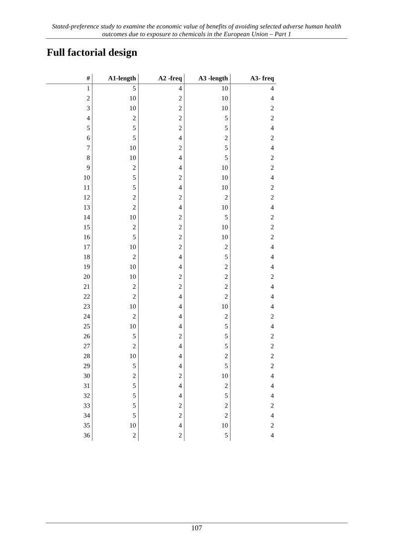
Stated-preference study to examine the economic value of benefits of avoiding selected adverse human health outcomes due to exposure to chemicals in the European Union – Part 1
107
Full factorial design
# A1-length A2 -freq A3 -length A3- freq 1 5 4 10 4 2 10 2 10 4 3 10 2 10 2 4 2 2 5 2 5 5 2 5 4 6 5 4 2 2 7 10 2 5 4 8 10 4 5 2 9 2 4 10 2
10 5 2 10 4 11 5 4 10 2 12 2 2 2 2 13 2 4 10 4 14 10 2 5 2 15 2 2 10 2 16 5 2 10 2 17 10 2 2 4 18 2 4 5 4 19 10 4 2 4 20 10 2 2 2 21 2 2 2 4 22 2 4 2 4 23 10 4 10 4 24 2 4 2 2 25 10 4 5 4 26 5 2 5 2 27 2 4 5 2 28 10 4 2 2 29 5 4 5 2 30 2 2 10 4 31 5 4 2 4 32 5 4 5 4 33 5 2 2 2 34 5 2 2 4 35 10 4 10 2 36 2 2 5 4

Stated-preference study to examine the economic value of benefits of avoiding selected adverse human health outcomes due to exposure to chemicals in the European Union – Part 1
108
Descriptive statistics (variables not included in the model)
Table III.1 – Perception of respondent’s present income by country
Czech United
Kingdom Netherlands Italy pooled
Living comfortably on present income 10.0% 22.0% 25.1% 6.7% 15.3%
Coping on present income 46.3% 43.4% 46.5% 42.9% 44.6%
Finding it difficult on present income 28.8% 24.8% 19.2% 31.3% 26.5%
Finding it very difficult on present income
14.9% 9.9% 9.2% 19.2% 13.6%
Total 900 984 684 991 3559
Subjective perception of respondent’s present income and how easy s/he can cope on it was investigated using four distinct categories, and the results show that there are substantial differences in the subjective perception of present income among countries. The share of people who manage to cope on or live comfortably on their present income is more than a half of the sample in all countries except Italy, where the more negative subjective perception of the personal income seems to be consistent with underrepresentation of higher personal income categories (quantiles). On the contrary, the largest share of these two categories is in the Netherlands (25.1% and 46.5%, respectively).
Table III.2 – Size of the municipality
Czech United
Kingdom Netherlands Italy pooled
up to 199 inhabitants 2.0% 3.9% 0.7% 1.8% 2.2%
200 to 499 inhabitants 5.1% 3.5% 0.6% 0.6% 2.5%
500 to 999 inhabitants 8.2% 3.4% 0.4% 2.1% 3.6%
1 000 to 1 999 inhabitants 6.1% 6.2% 2.9% 4.2% 5.0%
2 000 to 4 999 inhabitants 10.8% 8.3% 5.6% 10.1% 8.9%
5 000 to 9 999 inhabitants 7.9% 8.3% 7.3% 13.4% 9.4%
10 000 to 19 999 inhabitants 9.5% 12.2% 14.6% 14.4% 12.6%
20 000 to 49 999 inhabitants 13.3% 13.3% 19.6% 18.0% 15.8%
50 000 to 99 999 inhabitants 10.7% 11.3% 19.3% 9.9% 12.3%
100 000 to 999 999 inhabitants 13.4% 16.8% 26.6% 14.9% 17.3%
1 milion or more inhabitants 13.1% 12.9% 2.6% 10.8% 10.4%
Total 904 1006 700 1024 3634
In all countries, most of the respondents in the sample live in the category of municipalities from 100,000 to 999,999 inhabitants. Very different are the sample shares of low size municipalities among countries: while the share of residents of small municipalities up to 999 inhabitants is very low in the Netherlands and Italy, this type of residency is more common in the Czech Republic and United Kingdom. Around 28% of the pooled sample lives in large cities over 100,000 inhabitants.

Stated-preference study to examine the economic value of benefits of avoiding selected adverse human health outcomes due to exposure to chemicals in the European Union – Part 1
109
The largest municipality category is covered by more than 10% of the country samples, except for the Netherlands. Two largest Netherland cities, Amsterdam and Rotterdam, had according to latest available EUROSTAT statistics 790,110 and 616,260 inhabitants in 2012, respectively (EUROSTAT, 201436), and the largest size category of municipality should not be therefore covered within the sample at all. However, Amsterodam exceeds the limit of the last category when perceived as greater city of Amsterdam (1,021,754 inhabitants), and Rotterdam almost reaches the limit as a greater city (977,584 inhabitants, ibid.) and some respondents residing in these municipalities may have therefore stated their residencies in the largest category “1 million or more inhabitants”.
Table III.3 – Donation of money to a charity or non-profit organization in the past 12 months Czech United Kingdom Netherlands Italy pooled
Yes 44.4% 72.1% 54.7% 45.3% 54.3%
To have an idea how much money are respondents used to voluntarily donate, we included a direct question on donation of money to a charity or non-profit organization in the past 12 months. There are significant differences among countries. Whereas 72.1% of respondents in the UK sample answered positively, it was only about 45% in the Czech and the Italian sample.
Table III.4 – Coverage of respondent’s health care: dental health care
Czech United
Kingdom Netherlands Italy pooled
Fully or almost fully covers 24.5% 20.6% 19.9% 6.3% 17.9%
Does not fully cover 49.9% 26.6% 51.5% 17.8% 37.2%
Does not cover 14.4% 38.6% 22.0% 66.8% 34.7%
Don’t know 11.1% 14.2% 6.6% 9.2% 10.2%
The situation concerning the coverage of dental health care by the health insurance is completely different. Much often it is reported as not covered at all or not fully covered; the former category being the most frequent in the UK and Italy. The differences among countries are also apparent.
36 EUROSTAT (2014): Population on 1 January by age groups and sex - cities and greater cities. On-line. URL:<
http://ec.europa.eu/eurostat/product?code=urb_cpop1>. Accessed on 27th February 2014.

Stated-preference study to examine the economic value of benefits of avoiding selected adverse human health outcomes due to exposure to chemicals in the European Union – Part 1
110
WTP estimates WTP for avoiding individual illnesses (truncation strategy I, parametric estimates, lognormal, euro per case)
illness country frequency length mean WTP median WTP S.E. illness country frequency length mean WTP median
WTP S.E.
A pooled (1x/yr) (1yr) 226.2 145.0 3.05 A3 pooled 2x/yr. 2yrs 303.8 182.8 6.60
A cz (1x/yr) (1yr) 228.2 141.0 5.64 A3 pooled 2x/yr. 5yrs 352.4 210.7 6.08
A en (1x/yr) (1yr) 190.5 118.7 4.74 A3 pooled 2x/yr. 10yrs 441.5 260.6 10.45
A it (1x/yr) (1yr) 301.2 187.1 7.21 A3 pooled 4x/yr. 2yrs 347.6 205.6 7.52
A nl (1x/yr) (1yr) 204.0 126.5 6.86 A3 pooled 4x/yr. 5yrs 396.4 239.9 6.87
C pooled (1x/yr) (1yr) 492.2 312.2 5.94 A3 pooled 4x/yr. 10yrs 505.0 303.6 11.73
C cz (1x/yr) (1yr) 416.5 271.3 9.59 A3 cz 2x/yr. 2yrs 300.5 176.5 8.75
C en (1x/yr) (1yr) 534.1 346.2 11.98 A3 en 2x/yr. 2yrs 288.7 171.6 8.33
C it (1x/yr) (1yr) 582.2 365.6 13.32 A3 it 2x/yr. 2yrs 360.5 221.5 10.51
C nl (1x/yr) (1yr) 399.2 265.7 12.05 A3 nl 2x/yr. 2yrs 246.2 150.0 8.92
A1 pooled 2x/yr. (1yr) 292.0 186.0 5.11 A3 cz 2x/yr. 5yrs 345.2 201.9 9.12
A1 pooled 4x/yr. (1yr) 321.5 204.9 5.49 A3 en 2x/yr. 5yrs 331.6 203.1 8.53
A1 cz 2x/yr. (1yr) 289.2 180.4 7.61 A3 it 2x/yr. 5yrs 414.1 253.9 10.74
A1 en 2x/yr. (1yr) 250.9 161.5 6.57 A3 nl 2x/yr. 5yrs 282.8 168.1 9.50
A1 it 2x/yr. (1yr) 357.5 229.1 9.34 A3 cz 2x/yr. 10yrs 434.9 255.3 13.51
A1 nl 2x/yr. (1yr) 257.9 164.0 8.65 A3 en 2x/yr. 10yrs 417.8 258.9 12.53
A1 cz 4x/yr. (1yr) 318.4 204.3 8.23 A3 it 2x/yr. 10yrs 521.8 304.7 15.77
A1 en 4x/yr. (1yr) 276.9 175.4 7.15 A3 nl 2x/yr. 10yrs 356.5 198.0 13.50
A1 it 4x/yr. (1yr) 394.6 250.2 10.25 A3 cz 4x/yr. 2yrs 344.9 202.4 9.84
A1 nl 4x/yr. (1yr) 286.1 182.8 9.38 A3 en 4x/yr. 2yrs 331.6 195.3 9.52
A2 pooled (1x/yr) 2yrs 301.0 183.8 5.52 A3 it 4x/yr. 2yrs 414.7 242.1 12.25
A2 pooled (1x/yr) 5yrs 326.4 201.4 4.09 A3 nl 4x/yr. 2yrs 285.3 175.9 10.22
A2 pooled (1x/yr) 10yrs 373.5 228.7 7.65 A3 cz 4x/yr. 5yrs 396.1 239.6 10.18
A2 cz (1x/yr) 2yrs 303.1 178.1 8.22 A3 en 4x/yr. 5yrs 380.9 225.7 9.70
A2 en (1x/yr) 2yrs 277.3 169.1 7.24 A3 it 4x/yr. 5yrs 476.4 285.0 12.52
A2 it (1x/yr) 2yrs 362.3 221.8 9.77 A3 nl 4x/yr. 5yrs 327.8 194.4 10.85
A2 nl (1x/yr) 2yrs 256.1 156.2 8.76 A3 cz 4x/yr. 10yrs 499.1 307.5 15.09
A2 cz (1x/yr) 5yrs 328.0 203.2 7.74 A3 en 4x/yr. 10yrs 479.9 281.3 14.18
A2 en (1x/yr) 5yrs 300.1 181.7 6.80 A3 it 4x/yr. 10yrs 600.3 359.3 18.18
A2 it (1x/yr) 5yrs 392.5 238.3 9.15 A3 nl 4x/yr. 10yrs 413.1 253.4 15.35
A2 nl (1x/yr) 5yrs 278.2 177.2 8.65
A2 cz (1x/yr) 10yrs 374.0 227.0 10.53
A2 en (1x/yr) 10yrs 342.3 211.4 9.50
A2 it (1x/yr) 10yrs 448.3 273.6 12.62
A2 nl (1x/yr) 10yrs 319.2 184.7 11.31 Note: standard errors were estimated using the delta method.

Stated-preference study to examine the economic value of benefits of avoiding selected adverse human health outcomes due to exposure to chemicals in the European Union – Part 1
111
WTP for avoiding individual illnesses (truncation strategy II, pooled, euro per case)
illness frequency length non-parametric parametric - lognormal parametric - Weibull
mean WTP median WTP mean WTP median WTP S.E. mean WTP median WTP S.E. illness A 216.0 156 230.2 147.5 2.97 214.0 167.6 4.32 illness A1 2 269.5 212 279.1 185.1 4.84 273.3 208.6 7.48 4 286.4 225 301.2 201.5 5.12 285.5 218.0 7.57 illness A2 2 269.7 189 280.1 180.4 5.19 269.0 207.7 7.74 5 283.5 245 306.0 194.9 3.87 286.0 220.8 5.74 10 319.0 252 349.3 223.9 7.31 316.6 244.4 10.10 illness A3 2 2 239.6 192 275.6 176.4 6.01 249.4 186.6 8.60 4 2 277.6 212 318.9 199.9 6.93 289.6 216.7 10.01 2 5 317.3 270 311.5 200.3 5.45 293.9 219.9 8.20 4 5 354.0 265 360.7 232.7 6.28 341.5 255.5 9.49 2 10 364.6 276 382.0 240.6 9.21 386.3 289.0 14.92 4 10 456.6 315 442.6 282.2 10.53 449.3 336.2 17.03 illness C 453.9 314 458.4 302.3 5.50 450.9 331.0 9.04
Notes: Estimates from parametric models were selected based on AIC and Weibull models performed better for illnesses A and A2 while lognormal models performed better for illnesses A1, A3 and C. Standard errors were estimated using the delta method.

Stated-preference study to examine the economic value of benefits of avoiding selected adverse human health outcomes due to exposure to chemicals in the European Union – Part 1
112
Lower bound WTP for avoiding individual illnesses (truncation strategy I, parametric, lognormal, euro per case)
illness country frequency length non-zero probability
mean WTP
median WTP illness country frequency length non-zero
probability mean WTP
median WTP
A pooled (1x/yr) (1yr) 0.08 173.3 91.2 A3 pooled 2x/yr. 2yrs 0.05 237.5 121.4
A cz (1x/yr) (1yr) 0.05 158.3 84.6 A3 pooled 2x/yr. 5yrs 0.04 272.9 139.6
A en (1x/yr) (1yr) 0.08 142.3 76.0 A3 pooled 2x/yr. 10yrs 0.05 275.3 140.8
A it (1x/yr) (1yr) 0.06 219.6 117.3 A3 pooled 4x/yr. 2yrs 0.05 316.3 161.8
A nl (1x/yr) (1yr) 0.14 169.6 90.6 A3 pooled 4x/yr. 5yrs 0.05 352.1 180.1
C pooled (1x/yr) (1yr) 0.04 390.9 217.2 A3 pooled 4x/yr. 10yrs 0.05 404.6 206.9
C cz (1x/yr) (1yr) 0.02 310.9 175.1 A3 cz 2x/yr. 2yrs 0.03 219.2 112.8
C en (1x/yr) (1yr) 0.04 424.8 239.3 A3 en 2x/yr. 2yrs 0.04 224.9 115.7
C it (1x/yr) (1yr) 0.04 465.7 262.4 A3 it 2x/yr. 2yrs 0.05 281.1 144.6
C nl (1x/yr) (1yr) 0.09 336.9 189.8 A3 nl 2x/yr. 2yrs 0.11 214.5 110.4
A1 pooled 2x/yr. (1yr) 0.06 224.7 123.9 A3 cz 2x/yr. 5yrs 0.03 253.5 130.4
A1 pooled 4x/yr. (1yr) 0.05 247.6 136.5 A3 en 2x/yr. 5yrs 0.04 260.1 133.8
A1 cz 2x/yr. (1yr) 0.03 209.8 116.7 A3 it 2x/yr. 5yrs 0.05 325.1 167.3
A1 en 2x/yr. (1yr) 0.05 192.7 107.2 A3 nl 2x/yr. 5yrs 0.11 248.0 127.6
A1 it 2x/yr. (1yr) 0.05 273.2 152.0 A3 cz 2x/yr. 10yrs 0.03 323.0 166.2
A1 nl 2x/yr. (1yr) 0.11 218.4 121.5 A3 en 2x/yr. 10yrs 0.04 331.4 170.5
A1 cz 4x/yr. (1yr) 0.03 231.8 129.0 A3 it 2x/yr. 10yrs 0.05 414.2 213.1
A1 en 4x/yr. (1yr) 0.05 212.9 118.5 A3 nl 2x/yr. 10yrs 0.11 316.0 162.6
A1 it 4x/yr. (1yr) 0.05 302.0 168.0 A3 cz 4x/yr. 2yrs 0.03 253.9 130.6
A1 nl 4x/yr. (1yr) 0.10 241.4 134.3 A3 en 4x/yr. 2yrs 0.03 260.6 134.1
A2 pooled (1x/yr) 2yrs 0.06 231.2 121.8 A3 it 4x/yr. 2yrs 0.04 325.6 167.5
A2 pooled (1x/yr) 5yrs 0.06 253.8 133.7 A3 nl 4x/yr. 2yrs 0.10 248.5 127.8
A2 pooled (1x/yr) 10yrs 0.05 296.5 156.2 A3 cz 4x/yr. 5yrs 0.03 293.6 151.1
A2 cz (1x/yr) 2yrs 0.04 216.6 115.0 A3 en 4x/yr. 5yrs 0.03 301.3 155.0
A2 en (1x/yr) 2yrs 0.04 206.4 109.6 A3 it 4x/yr. 5yrs 0.04 376.6 193.8
A2 it (1x/yr) 2yrs 0.06 278.8 148.0 A3 nl 4x/yr. 5yrs 0.10 287.3 147.8
A2 nl (1x/yr) 2yrs 0.12 218.6 116.0 A3 cz 4x/yr. 10yrs 0.02 374.1 192.5
A2 cz (1x/yr) 5yrs 0.04 237.6 126.1 A3 en 4x/yr. 10yrs 0.03 383.9 197.5
A2 en (1x/yr) 5yrs 0.04 226.4 120.2 A3 it 4x/yr. 10yrs 0.04 479.8 246.9
A2 it (1x/yr) 5yrs 0.06 305.8 162.3 A3 nl 4x/yr. 10yrs 0.10 366.1 188.4
A2 nl (1x/yr) 5yrs 0.11 239.8 127.3
A2 cz (1x/yr) 10yrs 0.03 277.2 147.2
A2 en (1x/yr) 10yrs 0.04 264.2 140.3
A2 it (1x/yr) 10yrs 0.05 356.8 189.4
A2 nl (1x/yr) 10yrs 0.10 279.7 148.5

Stated-preference study to examine the economic value of benefits of avoiding selected adverse human health outcomes due to exposure to chemicals in the European Union – Part 1
113
Lower bound WTP for avoiding individual illnesses (truncation strategy II, parametric, lognormal, euro per case)
illness frequency length non-zero probability mean WTP median WTP illness A 0.08 170.3 92.1 illness A1 2 0.05 215.5 123.6 4 0.05 232.0 133.0 illness A2 2 0.06 213.1 117.5 5 0.06 235.8 130.0 10 0.05 279.1 153.9 illness A3 2 2 0.05 214.9 117.4 2 5 0.05 245.3 134.0 2 10 0.06 305.7 167.0 4 2 0.04 248.8 136.0 4 5 0.04 284.0 155.2 4 10 0.05 354.0 193.4 illness C 0.04 362.0 209.1