Appendix 5e: Understanding Customer Values …...This work package used stated preference methods to...

Appendix 5e: Understanding Customer

Values_ Stated Preference Report

1

PR19 Understanding Customer Values: Work Package 1 – First Round Stated Preference

Prepared for Yorkshire Water

Acknowledgements

AECOM and DJS Research would like to thank Professor Michael Ward (Monash University) for providing peer

review of the work undertaken for this work package.

Quality information

Document name Prepared for Prepared by Date Approved by

Work Package 1

Draft Report Yorkshire Water

Ali Sims

(DJS Research)

Matt Prince

(DJS Research)

Rachel Waddington

(DJS Research)

01/11/17 Chris White

(AECOM)

AECOM Infrastructure & Environment UK Limited (AECOM) has prepared this Report for the sole use of Yorkshire Water (“Client”) in accordance with the terms and conditions of appointment. No other warranty, expressed or implied, is made as to the professional advice included in this Report or any other services provided by AECOM. This Report may not be relied upon by any other party without the prior and express written agreement of AECOM. Where any conclusions and recommendations contained in this Report are based upon information provided by others, it has been assumed that all relevant information has been provided by those parties and that such information is accurate. Any such information obtained by AECOM has not been independently verified by AECOM, unless otherwise stated in the Report.

2

Contents

Contents ........................................................................................................................................................................... 2

Work Package 1 – First Round Summary ...................................................................................................................... 0

Aims .................................................................................................................................................................................. 0

Method .............................................................................................................................................................................. 0

Results .............................................................................................................................................................................. 2

Implications ...................................................................................................................................................................... 5

Appendix 1: PR19 Understanding Customer Values - Approach, Methodology & Results Aecom & DJS Report

0

DJS Research Ltd. 2017

Work Package 1 – First Round

Context

The aim of this project is to undertake primary research to ascertain the values that Yorkshire Water (YWS)

customers place on changes in service measures such as interruptions to supply or drinking water failures.

These values will then be used to populate the Decision Making Framework (DMF) in order to inform the

investment planning process and support the wider Outcome Delivery Incentives (ODI) work stream.

In light of Ofwat’s recommendations for improving the approach to understanding customer’s values in

PR19, the project includes six work packages (see Figure 1) which draw on a range of data to allow

methodological triangulation; whereby data of different types are used to cumulatively refine and validate

research outputs.

Figure 1. Overview of the six work packages

Aims

The aim of this work package is to try to estimate the values YWS’ customers and business consumers

place on changes in service measures using a stated preference survey. Values are derived for the

attributes included in the survey with the view that these will be compared to costs to help determine

potential areas for investment at PR19. The specific questions which this work package aims to answer are

as follows:

• What is the willingness-to-pay (WTP) amongst YWS customers for changes in service

measures?

• How does WTP differ across socio-economic group, age, lifestage, vulnerable customers, low

income customers, location in the region, and those who have experienced a service measure

failure?

• How do use and non-use values compare for environment related service measures (i.e.

bathing water quality, river water quality, pollution incidents, and land conservation)?

Method

This work package involved undertaking two surveys with YWS customers; both of which were quantitative

surveys conducted via a combination of Computer Aided Personal Interviewing (CAPI) and online panel. A

total of 1,020 household and 542 business surveys are included in the analysis for this work package. The

make-up of household surveys was based on a pre-agreed sample structure in order to provide a

1


representative sample of bill paying household customers in the YWS region by age, socio-economic group,

gender, region, and metered status. Business interview quotas were based on region, sector, and the

number of employees in the business.

This work package used stated preference methods to undertake quantitative customer research. Stated

preference methods attempt to directly elicit customer preferences for service priorities and improvements

by asking choice or direct valuation questions through survey questionnaires and interviews. A choice

experiment (CE) approach of stated preference was adopted in this work package.

The stated preference survey design implemented in this work package was composed of the specification

of four fundamental components:

• Water quality, water supply, sewerage services, the environment and their levels for the CE

questions

• The experimental design for the CE exercise

• The strategy for sampling and implementing the survey

In addition, the inclusion of attitudinal questions acting as covariates for the modelling (used to estimate

the contribution of use and non-use values to customer’s WTP) aimed to reduce issues of double counting

of values within the DMF.

To assist in customer understanding of the concepts being presented to them a visually engaging set of

show cards and choice cards were developed. Examples of the design are shown in Figures 1 and 2 below.

Figure 1: Show card example

Figure 2: Choice card example

2


Customer understanding of the show cards and choice cards was tested in the cognitive phase, and customer understanding of the concepts was high.

Results

Household

Table 1 below summarises the choice behaviour observed with the household customer samples across

the four service area blocks. For each choice experiment, household customers were shown four sets of

three choices, the status quo and two alternative options with different bill impacts associated with each.

The alternative options were chosen, at random, from 96 alternatives per service block area.

Table 1. Choice frequencies for household samples

Service area Status quo Alternative 1 Alternative 2

Water quality 66% 17% 17%

Supply of water 57% 21% 22%

Sewerage services 54% 23% 23%

Environment 51% 24% 25%

Table 2. Proportion of serial status quo choices and bill reduction option choices

Service area Always choose status

quo

Always choose bill

increases

Always choose bill

reductions


Supply of water 33% 13% 9%



Table 1 reveals a very high level of choice of the status quo option within each of the service area blocks

having a higher level of choice for the status quo option than alternatives combined. There is some level of

trading with the alternative hypothetical options noted, particularly in the environmental water service

option.

Table 2 meanwhile, shows around a third of respondents consistently choose the status quo when given

multiple choices.

The final WTP and willingness-to-accept (WTA) estimates for household customers, based on a non-linear

model, are summarised in

Table 3. In almost all of the areas considered, the level of WTA is greater than the level of WTP for the

greatest service decrease or increase.

3


Table 3. Household willingness-to-pay and willingness-to-accept estimates

Service

area Service level attribute

WTP / WTA

-1 +1 +2 +3

Water quality

Poor water pressure: number of properties below standard

pressure -£1.37 £0.48 £0.82 £1.05

Drinking water quality: proportion of samples of tap water

that will pass the DWI’s requirement for chemical &

biological content

-£1.11 £0.49 £1.66 £2.15

Taste, smell & colour of drinking water: total number of

water quality contacts -£1.49 £2.09 £3.74 £4.40

Supply of

water

Unexpected supply interruption of 3–6 hours: total

properties affected -£0.82 £0.20 £0.61 £0.77

Leakage -£1.09 £0.44 £0.72 £0.83

Water use restrictions e.g. hose pipe ban -£0.50 £0.26 £0.26 £0.29

Sewerage

services

Sewer flooding inside properties: number of incidents per

year -£1.13 £0.57 £1.19 £1.43

Sewer flooding outside properties: number of incidents per

year -£0.82 £0.28 £0.46 £0.64

Properties subjected to chronic (seasonal) unbearable

smells from sewers and treatment works: complaints to

YWS per year

-£0.21 £0.40 £0.60 £0.66

Environment

Number of bathing beaches meeting ‘Good’ or ‘Excellent’

standard -£0.91 £0.32 £0.48 £0.49

Length of rivers in Yorkshire improved (%) -£0.82 £0.83 £1.14 £1.35

Category 3 pollution incidents: number of minor incidents

that have a minimal impact on the quality of water in the

area

-£0.43 £0.33 £0.60 £0.82

Area of land conserved or improved by Yorkshire Water:

hectares -£0.56 £0.39 £0.53 £0.58

4


Business

Table 4 and

Table 5 summarise the choice behaviour observed with the business customer samples across the four

service area blocks. For each choice experiment business customers were shown four sets of three

choices, the status quo and two alternative options with different bill impacts associated with each. The

alternative options were chosen, at random, from 96 alternatives per service block area.

Table 4. Choice frequencies for business samples

Service area Status quo Alternative 1 Alternative 2


Supply of Water 49% 25% 26%



Table 5. Proportion of serial status quo choices and bill reduction option choices

Service area Always choose

status quo

Always choose bill

increases

Always choose bill

reductions





Table 4 reveals a very high level of choice of the status quo option with two service area blocks having a higher level of choice for the status quo option than the alternatives combined. Environmental services have the largest deviation from the status quo.

Table 5 shows about a third of business respondents consistently choose the status quo when given multiple choices. The remainder of respondents in

Table 5 select different options across the CE sets within the blocks.

The final WTP and WTA estimates for business customers, based on the non-linear model are summarised

in Table 6. In almost all of the areas considered, the level of WTA is greater than the level of WTP for the

greatest service decrease or increase.

5


Table 6. Business willingness-to-pay and willingness-to-accept estimates

Service

area Service level attribute

WTP / WTA

-1 +1 +2 +3

Water quality

Poor water pressure: number of properties below standard

pressure -0.20% 0.20% 0.27% 0.29%

Drinking water quality: proportion of samples of tap water

that will pass the DWI’s requirement for chemical &

biological content

-0.38% 0.26% 0.37% 0.40%

Taste, smell & colour of drinking water: total number of

water quality contacts -0.43% 0.57% 1.21% 1.41%

Supply of

water


properties affected -0.23% 0.11% 0.26% 0.28%

Leakage -0.37% 0.13% 0.24% 0.26%

Water use restrictions e.g. hose pipe ban -0.05% 0.08% 0.15% 0.21%

Sewerage

services


year -0.28% 0.12% 0.26% 0.34%

Sewer flooding outside properties: number of incidents per

year -0.12% 0.12% 0.20% 0.21%


smells from sewers and treatment works: complaints to

YWS per year

-0.08% 0.12% 0.25% 0.29%

Environment


standard -0.17% 0.13% 0.16% 0.21%

Length of rivers in Yorkshire improved (%) -0.35% 0.40% 0.73% 0.74%

Category 3 pollution incidents: number of minor incidents

that have a minimal impact on the quality of water in the

area

-0.23% 0.17% 0.33% 0.45%

Area of land conserved or improved by Yorkshire Water:

hectares -0.20% 0.20% 0.27% 0.11%

Implications

For both the household and business surveys, in terms of statistical validity, the models provide a good fit

to the data. The reliability of the analysis is supported by the validity assessments. There is a high tendency

to stay with the status quo, especially for Water Quality, amongst household and business customers. This

trend is more marked than in PR14 with approximately a third of customers sticking with the status quo

throughout the PR19 survey; perhaps indicating either a fear of change in uncertain economic times or a

satisfaction with the existing levels of service.

Across all attributes except for Taste, Colour, and Smell of Drinking Water, the Willingness to Accept

amongst household customers is greater than the Willingness to Pay. The picture is similar amongst

businesses for the Willingness to Pay greater for Taste, Colour and Smell of Drinking Water. For Sewer

Flooding outside properties and Length of Rivers in Yorkshire Improved there is no difference between

Willingness to Accept and Willingness to Pay.

6


Analysis of WTP estimates and data by sub-groups including demographics, socio-economic groups,

vulnerable definitions, and prior service experiences, shows the WTP ranking per service measure

remaining largely consistent across analysis groups, with Taste, Colour, and Smell of Drinking Water

consistently having the highest WTP estimate value, regardless of group. There are, however, a number

of significant WTP differences when service measure outcomes are compared (see Appendix 2: Results).

Levels of Willingness to Pay are lower than in previous years; with 42% of household customers falling into

the Financially Vulnerable category and high preferences for the status quo, this study is reflective of the

current economic climate and such constraints on WTP should be taken into account when investment

planning.

For PR19, further analysis has been conducted to express the Total Economic Value in terms of ‘use’ and

‘non-use’ values. Non-use WTP estimates are higher for the environmental service areas than the other

service areas. Conversely, the Use WTP estimates tend to be lower for the environmental service areas

compared to the other service areas.

When looking at vulnerable customer definitions it becomes apparent that WTP differences are largely

isolated to issues of water quality and supply of water, while sewerage services and environmental service

measures throw up fewer differences. For all of these differences, customers not classed as vulnerable

have higher WTP estimates than customers who might be considered vulnerable. The suggestion here is

that while WTP preferences might be broadly in line, the additional amount that customers in vulnerable

circumstances are willing to pay on top of the expected bill amount is lower than those not in vulnerable

circumstances. This applies whether they are financially vulnerable or whether their vulnerability is health-

related. This is likely to be because there is so much correlation between the two vulnerabilities with

financial circumstances thus driving WTP. Similarly, customers in lower SEG groups have lower WTP

estimate amounts across a number of service measures than higher SEG customers.

When looking at WTP differences by service experience, it is interesting to note that the type of experience

appears to dictate the extent to which significant differences occur. For example, when comparing

customers who have experienced low water pressure with those who haven’t, only one significant difference

occurs across the 13 service measures. However, by contrast, when looking at sewer flooding inside the

property on an experienced vs. not experienced basis, 11 significant differences occur. Customers

experiencing the following service failures have a higher WTP for this service measure, than those who

haven’t:

• Sewer flooding inside properties

• A leaking water supply pipe close to your property

• Restriction on how you can use water e.g. a hosepipe ban

0


1


Contents This document has been prepared by DJS Research Ltd (DJS), consisting of the

following project team:

Ali Sims – Research Director

Rachel Waddington – Statistician

Matt Prince – Research Manager

A table of contents is provided below:

Appendix 1 - method 2

Appendix 2 – results and findings – household 23

Appendix 2 – results and findings – business 77

2


Appendix 1 - approach Design and interviewing summary

Surveys were designed by DJS Research, Yorkshire Water and Aecom, with input

from London Economics and the Yorkshire Water Customer Forum Group. A detailed

outline of the conceptual approach to the survey design is provided in the Conceptual

summary (p.13) section.

Prior to conducting the main fieldwork, a pilot phase testing both the household and

business customer surveys was conducted in August 2017.

The pilot phase of the fieldwork consisted of 10 CAPI interviews and 50 online

interviews with household customers and 5 CAPI interviews with business customers.

The purpose of the pilot phase was to validate the survey structure and design, with

the aim of refining the approach and questions ahead of the main fieldwork period.

CAPI interviews in the pilot phase were conducted by experienced interviewers who

were accompanied by a member of the DJS Research team, who were present to

observe the interviews.

The findings of the pilot phase suggested the surveys were well understood by

customers (both household and business), but that some refinement of approach was

required to optimise the survey design and validity.

Main stage surveys

Across both surveys pictorial show cards and choice experiment grids were created

to aid respondent understanding of the concepts displayed (examples of the show

cards are shown from p.21). In addition, show cards were created to deliver

information to respondents about Yorkshire Water’s responsibilities. CAPI

respondents were provided with bound, laminated booklets of the show cards and

example grids, while online respondents were shown ‘dynamic’ on-screen images

which re-sized according to the device used.

Household survey

The technical aspects of the survey concept are discussed later in this report from

p.12 This section outlines the final survey design mechanics. The final household

survey consisted of six main question sections:

• Screening questions to establish respondent suitability for the survey:

o The respondent does not work in any conflict professions (Journalism,

advertising, market research, PR, the water industry or the Environment

Agency)

o The respondent has their water and sewerage services provided by

Yorkshire Water;

o And, has sole or joint responsibility for paying the water bill

3


• Attitudinal and experience questions to improve the stated preference

field and to provide use and non-use values.

• Choice experiment blocks to establish stated preference across four service

areas

o Respondents were provided with show cards for each of the service level

attributes (discussed and shown in detail from p.21), before being asked

to make their choices;

o Respondents were shown 3 choice cards per service area (12 choices in

total). Prior to making their choices, respondents were provided with an

example choice card and an explanation of the questions they would be

asked. Each respondent was provided with 3 options per choice – two

price changing options (stated in monetary value) and one ‘no change’

option.

• A whole package choice experiment where respondents were provided

with 2 choices – top level service provision for each service level attribute and

a randomly assigned additional bill value, and Yorkshire Water’s stated

performance for 2020 for each service level attribute – ‘no change’

• Choice experiment validation questions to establish the extent to which

the respondent had understood the concepts and questions they were faced

with, and to understand the rationale behind the respondent’s decision making

• Classification and demographic questions to provide the basis for sub-

group analysis

Business survey

The business survey followed the same approach in respect of the choice

experiment blocks, and the whole package choice experiment – although here

the stated change was expressed in terms of a percentage bill change as opposed to

the monetary changes shown for household customers.

Other elements of the survey were tailored accordingly for a business audience

• Screening questions to establish;

o that the respondent has responsibility for the water bill within the

business

o the business is supplied by Yorkshire Water (even if not billed by,

following commercial water reform in April 2017)

• Classification questions to establish the business sector and the business

size (in respect of employee numbers)

• Importance of water questions to establish the importance of water to the

day to day running and operation of the business

4


Interviewing

Interviews across both the household and business surveys were conducted using

the following approaches:

• Computer Aided Personal Interviewing (CAPI): surveys were conducted

in the customer’s home/business on a tablet device and were interviewer led.

Interviewers were provided with quotas, and sampling points by region were

designed to provide a robust representation of customers across Yorkshire.

• Online panel interviews: surveys were completed by the respondent online.

Quotas on participation were set to ensure a representative sample of

customers and respondents were sourced through panel providers.

The use of a CAPI approach, in conjunction with online panel, was used in order to

reach customers and communities that may be underrepresented online.

Interviews were conducted from 31st August to 9th October 2017.

Sample

Household

The following split of interviews across household quota groups was achieved:

Table 7: Household interviews

WP1 – Household

CAPI

WP1 – Household

online

WP1 – Household

total

Male 46 440 486

Female 68 461 529

Prefer not to say /

Transgender / Non-binary 0 5 5

18-34 16 151 167

35-44 11 149 160

45-54 26 180 206

55-64 22 183 205

65+ 39 243 282

North Yorkshire 23 144 167

East Yorkshire 10 107 117

South Yorkshire 34 230 264

West Yorkshire 47 425 472

5


ABC1 23 479 502

C2DE 91 427 518

Metered 41 511 552

Unmetered 73 395 468

Total 114 906 1020

Final sample splits on gender, region, SEG and metered status all fell within 5% of

original sample quota targets. The final numbers on age show a slight over-

representation of 55-64s, and a slight underrepresentation of under 35s – however,

given the overall profile of the sample make-up it was decided that no weighting of

data was necessary.

Business

Table 8: Business interviews

WP1 – Business

CAPI

WP1 Business

online

WP1 – Business

total

North Yorkshire 34 41 75

East Yorkshire 30 20 50

South Yorkshire 101 49 150

West Yorkshire 129 100 229

Micro (0-9 employees) 228 72 300

Small (10-49 employees) 65 40 105

Medium (50-249 employees) 3 60 63

Large (250+ employees) - 74 74

Industrial 68 85 153

Commercial 140 56 196

Public sector 57 42 99

Other (3rd sector, arts &

entertainment etc.) 31 63 94

6


Total 296 246 542

Region wasn’t recorded for all businesses, due to complications of multi-site

organisations, operating across multiple regions of Yorkshire and the rest of the UK.

In order to gain access to smaller businesses, that might not be well represented in

online panels, the focus of the CAPI interviews was on micro and small businesses.

Yorkshire Water online community

In addition to the main stage interviews, the online questionnaire was opened to

members of Yorkshire Water’s online community. Members were invited to take part

in the survey via a survey link. Overall, 175 interviews were completed via this

method. The results of these interviews are used for comparison with the willingness

to pay results of the total sample of the main stage surveys in Appendix 2 of this

report.

Conceptual summary

This section provides an overview of the concepts and theories that underlie the

stated preference methods. The section is written as a non-technical piece for a wide

audience, however, some technical complexity is both inevitable and useful.

Estimating customer willingness to pay and accept

Quantitative research as undertaken in this study involves designing a survey that

elicits the preferences of two separate samples representative of YW household and

business customers. During the survey, respondents are asked to trade off

maintained or improved quality of water and wastewater services against increases

in the water bill. This trade off results in what economic literature calls Willingness to

Pay (WTP). If individuals are willing to pay to avoid a decline (maintenance) and to

secure an improvement, the survey results in positive and significant WTP estimates.

Respondents are also asked to trade off the declining quality of water and waste

water services against a decline in the water bill – if maintenance and improvement

investment is not necessary, bills will not need to increase to pay for them. This

trade-off results in what economic literature calls Willingness to Accept Compensation

(WTA). If individuals are willing to accept bill declines as compensation to tolerate

service declines and to forgo service improvements, the survey results in positive

and significant WTA estimates.

The bill impacts that respondents are shown are based on the expected costs to

consumers associated with the investments necessary to improve the service.

Varying levels of bill impacts are presented to respondents. The advantage of using

water bills to express the trade-offs is that it is familiar to respondents and the actual

vehicle through which service changes will come about. It also allows for WTP and

WTA to be expressed in monetary terms. This allows for the benefits (or costs) of

service changes to the customers to be compared directly to the cost of providing

7


service changes (or avoided costs for service decline) to the company. In other

words, WTP and WTA are estimated to make Cost Benefit Analysis (CBA) possible.

The main purpose of this research is to estimate the Total Economic Value (TEV) for

each water service. Further analysis then aims to express this TEV in terms of ‘use’

and ‘non-use’ values. ‘Use value’ relates to how customers use water as a private

good and are therefore likely to be concerned about the quality and security of the

Supply of Water and wastewater management. Customers may also benefit from

services that affect the quality of the environment either because they directly use

the environment (e.g. for recreation) or because good environmental quality affects

their quality of life. This measure is called ‘indirect use value’. Finally, customers may

value YW’s services for the benefit of others (altruism value), for future generations

(bequest value) and, especially for environment-related services, for the benefit of

the environment (existence value). Together, these motivations are labelled as ‘non-

use values’.

All these use and non-use value components make up the Total Economic Value (TEV)

that valuation methods aim to estimate. There are two primary methods for

estimating customers’ WTP and WTA: revealed preference and stated preference.

This research uses stated preference methods. Stated preference studies are a

survey based approach that can be undertaken in two ways. Contingent valuation

(CV) directly asks respondents for their WTP or WTA for a change in the provision of

a good or service, while choice experiments (CE) ask respondents to state their most

preferred option from a range of choices and consequently infers their WTP or WTA

from these choices. In the context of this study, the choices are made between

individual services (or attributes) in different combinations with a price tag (water

bill amount) associated with each choice. This study uses a choice experiment

methodology due to the complex nature and number of water Service Measures and

varying levels that are investigated. Revealed preference has been used in Work

Package 3.

Stated preference choice experiments - summary

Choice modelling is underpinned by consumer demand theory, particularly the theory

of consumer behaviour following Lancaster (1966) and Rosen (1974). Consumer

demand theory assumes that the utility that customers receive from their water and

sewerage services derives from the characteristics of this good (e.g. the provision

they receive, the quality and safety of their water supply, and the disposal of waste

water).

CEs are used by economists to reveal individuals’ preferences and their willingness

to pay for particular attributes of goods and services. In a choice experiment,

individuals participating in a questionnaire survey are typically shown a choice card

depicting two or three alternative packages of service options. They are then asked

to identify the alternative that they prefer. Each alternative is based on a number of

service attributes (with associated bill impacts) that vary across the alternatives.

8


Information on Willingness to Pay and preferences across different service measures

are determined by observing the trade-offs that people make across repeated choices

based on different choice cards. The attributes of interest in this study are the service

measures that Yorkshire Water and its customers consider important, plus bill impact.

The varying levels involve potential increases or decreases to the current standard

of service provision for each service measure and the associated change to water

bills. Five levels were used in the experiment – two increases in standards for a

service measure and two decreases, in addition to the status quo where all service

measures remain at 2020 levels. The current situation was included because

consumers usually make choices in relation to what they currently have; rather than

making choices just between hypothetical alternatives. It is usual practice in choice

experiments to include the status quo, if the status quo is an option that the

consumer could choose.

In the CEs conducted in this survey, various combinations of service measure are

traded-off against each other and against changes to customers’ water bills. The first

four CEs (CE1-CE4) are each based on a ‘block’ of service measures (i.e. CE1 is based

on Water Quality; CE2 is based on Supply of Water; CE3 is based on Sewerage

Services; and CE4 is based on Environmental Factors. This is followed by a full-

package CE where the respondent is shown all 13 water services at the highest level

of improvements alongside the status quo with associated bill impact shown at

various levels. Each of CE1 to CE4 consisted of three separate choice exercises each

based around a set of three alternative combinations of attributes based on various

levels of service measure and a bill change. In each case respondents were asked to

choose their most preferred combination of service measure levels from those

offered. Repeated choices by customers (three for each of CE1-CE4) reveal the trade-

offs they are willing to make between service measures, their levels and their water

bills. Each set of choices contained the status quo option.

The inclusion of the status quo was important for customers to make an informed

choice. If they think about moving away from the status quo, then they consider the

alternatives and decide whether or not they offer an improvement in utility. Thus, in

the context of this study, customers might be assumed to consider whether or not

they are satisfied with the current water quality, water supply sewerage and

environmental service standards provided by YW and, if not, then to consider what

service measures they wished to see changed and how much they were willing to pay

for service improvements (or how much financial compensation they require for a

lower level of service).

In a CE it is assumed that individuals know their own preferences and are able to

choose which alternative scenario offers them the highest utility (a nested approach).

Thus, if an individual is assumed to choose alternative j over alternative k, if the

utility derived from attribute bundle j is greater than the utility derived from attribute

bundle k; i.e. if Uij > Uik, where Uij is the total utility associated with alternative j

9


and Uik is the total utility associated with alternative k. The utility function for

respondent i related to alternative j is specified as:

Uij = Vij + εij

where Vij is the ‘measurable’ systematic utility function observed by the analyst

because it is linkable to the attribute levels of each alternative (e.g. linked to the

levels of service they are shown) and εij is a random component, which is known to

the individual, but remains unobserved to the analyst. This random component (εij)

arises either because of randomness in the preferences of the individual or the fact

that we do not have the complete set of information available to the individual.

Figure 1 presents the different types of econometric models that are used to analyse

the respondents’ choices. These increase in their level of complexity and explanatory

power from Conditional Logit (CL) to Generalized Mixed Logit (GMXL) models.

Figure 1: Types of econometric modelling used

Model Description

Conditional Logit (CL)

model

This model explains the likelihood of an option being chosen by a respondent, explained by the attributes of the Water Service alone and does not include the

characteristics of the respondent.

Multinomial logit (MNL) model

This model explains the likelihood of an option being chosen by a respondent by the attributes of the Water Service and the characteristics of the respondent.

Nested logit

(NL) model

This is an extension of the above MNL model. It treats decisions as a ‘hierarchical’

choice, for example choosing whether or not they reject the status quo and then choosing between alternative improvement options.

Error corrected (EC) model

This model relaxes the MNL assumptions on the error term in relation to how a decrease in the likelihood of choosing an option is correlated to the chance of selecting an alternative option.

RPL Mixed logit (MXL) models

These improve upon the MNL models, addressing their limitations via a set of alternative models:

• Random Parameter Logit (RPL) model: the MNL model assumes that respondents’ choices are influenced by the same variables in the same way. In other words, the coefficients of the variables are the same over all respondents (i.e. homogeneity in preferences). The Random Parameter

Logit(RPL) model allows for the assumption that different variables influence individual respondents in different ways. In other words, the coefficients vary between individuals (i.e. heterogeneous preferences).

Generalized

Mixed Logit(GMXL)

The generalized mixed logit model developed by Fiebig et al (2010) is an extension of

the Random Parameter Logit model which allows for heterogeneity in both preference and scale which often coexist but observations have revealed that their importance varies in different choice contexts.

Linear or Non-linear WTP and WTA estimates

Our study design includes both service improvements and deteriorations for all

attributes and associated bill increases and reductions, respectively. This means we

are able to estimate both WTP for service improvements and WTA (compensation) to

tolerate service level decreases.

10


It is unlikely that there will be perfect symmetry in WTA and WTP estimates – where

symmetry means WTP for a +1 service level increase equals WTA for a -1 level of

service decrease. Specifically, it is typically observed that a loss or deterioration of a

unit of service is valued more highly than an equivalent gain in service level

This discrepancy between WTA and WTP can be examined by considering both linear

and nonlinear functions. A linear function would be consistent with symmetry,

whereas piecewise linearity – specifically a spline at the threshold between

deteriorations and improvements would provide evidence of asymmetry.

Willingness to pay (WTP) vs. Willingness to Accept (WTA)

Figure 2: WTP vs. WTA

Each of the models described in Fig 1 are linear models, in the sense that the same

coefficient estimate applies over the whole range of service levels from Level -2 to

Level +2). When considering non-linear models, we use a utility specification where

different service levels may have utility effects each represented by specific dummy

variable coefficients. In such models separate coefficients are estimated for each

level of service (-1, 0, 1, 2 and 3).

Comparing the ‘fit’ for each model

There is no single criterion by which a model can be identified as the ‘correct’ or ‘best’

model. Models are assessed on a wide range of criteria including:

11


• Econometric assumptions: criteria such as any perceived difference

between the status quo and alternatives by customers; how error components

are accounted for in the model; or allowed to vary across customers; linear or

non-linear functional relationships; etc.;

• Goodness-of-fit of the model: across various goodness-of-fit criteria,

including log-likelihood; AIC; BIC; HQIC; McFadden pseudo 𝑅2, Adj𝑅2; etc.;

• Positive or negative coefficients: do the signs conform to a priori

expectations: that is, as service levels improve does utility increase, and

conversely as service levels fall does utility decrease?

• Statistical significance of the coefficients: are the coefficients statistically

significant?

A pseudo-𝑅2 is a measure of goodness of fit: the higher the pseudo-𝑅2 value, the

greater the ability of the model to explain the choice data. A pseudo-𝑅2 value of 0.12

is considered good for CL models employing cross-sectional data (Breffle and Rowe,

2002).

Checking the validation of the estimates

An important component of the analysis of stated preference data is to assess

validity. Evidence in support of the validity of the results can be found in a variety of

ways. There are generally two types of validity tests that researchers employ in

stated preference exercises: content validity and construct validity.

Content validity

Content validity refers to whether the survey questionnaire succeeded in achieving

meaningful and accurate measures of the respondents’ WTP (or WTA) for the water

service being valued. Content validity can be affected by the information provided to

respondents on the good or service, the structure of the choice experiment, and the

change to customers’ annual water bills. The WTP and WTA values provided in this

analysis will always be estimates but, we can use some data from other questions in

the survey to determine if problems with content validity are evident.

It is important to identify if there are any systematic biases in responses (i.e. a

respondent always choosing the same option in a CE) or evidence of protest

responses). Other assessments of content validity include examining responses to

questions that assessed the level of the respondents’ understanding of the choice

experiments. In addition, for CAPI (Computer Aided Personal Interview) surveys

interviewers report on respondents’ understanding and ability to pick between the

options presented in the CE exercise and provide additional feedback about how

individual respondents have engaged with the task.

Construct validity

12


In addition to content validity, stated preference studies are often subjected to tests

of construct validity, which examine whether or not the results are consistent with

external evidence and expectation. Construct validity is generally broken down into

two categories: convergent validity and theoretical validity.

Convergent validity

Convergent validity refers to the comparison of WTP (or WTA) results for the same

goods or services derived by different methods. Our study uses the CE method to

estimate WTP and no other directly comparable stated preference method.

Theoretical validity

Theoretical validity involves testing the study results against the expectations

established by economic theory. One common application is to examine WTP

responses based on socio-economic and demographic factors that should influence

customers’ values. If the results show that WTP (or WTA) is dependent on these

variables, this provides further evidence that the results conform to expectations and

are theoretically valid.

For example, we expect to see that customers who are identified as ‘financially

vulnerable’ will be have lower WTP compared to respondent who are not financially

vulnerable.

Choice experiment blocks

The choice experiment blocks and service level attributes to be tested within the

survey were created and refined over a period of weeks by Yorkshire Water, Aecom

and DJS Research. Four choice experiment blocks were tested: water quality; water

supply; sewerage services, and environment.

Bill impacts for household customers were expressed as an actual amount, and for

business customers as a percentage change in their annual bill. The bill impacts in

the experimental design were derived from actual expected service development

costs.

The number of service measures was too great to include in one single CE: customers

would be unable to trade-off all simultaneously. Hence the service measures were

divided into four blocks based on how they impacted on services. These four blocks

of service measures formed the basis of CE1 to CE4 respectively. An experimental

design was produced for each of these blocks.

Designs that are both orthogonal (when the services that are being valued are

uncorrelated) and balanced (when each level occurs equally often) are often used in

choice experiments. However, it is more important in this exercise to maximize the

amount of information obtained. Thus, the selected scenarios, need to be the

combination which produces the most information for the model, given certain prior

information.

13


A full factorial design is not necessary in this exercise. A fractional factorial design

was used, which allow for the main effect of each service measure to be estimated;

and in some cases, second order interactions, where such interactions exist between

individual service measures.

For the ‘Water Quality’ block which had three service measures (Poor Water Pressure,

Drinking Water Quality and Taste, Smell and Colour of Drinking Water), plus bill

impact, a full factorial would have resulted in 54= 625 profiles or different

combinations of service measure and bill effect. Water Supply and Sewerage Services

would also have 625 profiles in the full factorial design.

For the Environmental block which had four service measures, plus BILL, a full

factorial would have resulted in 3,125 profiles.

An efficient design was produced for each block. For the Water Quality, Water Supply

and Sewerage Services blocks the efficient design resulted in 80 choice cards, each

consisting of two hypothetical alternatives, plus the status quo.

The two hypothetical alternatives were presented to the respondent in random order

(as option 1 or option 2) to avoid any positioning bias. The status quo measure was

always presented as option 3. This allowed of a quicker digestion of the information

presented to respondents.

The same set of choice cards were used with both domestic and business customers

with the slight difference in the way that bill impacts were presented.

The theoretical expectations, a priori of the results, would be that Utility values

increase in line with an increase in level for each Water Service, that is, all things

being equal, customers prefer services to be improved. At the same time, we also

expect that Utility values will decrease as water bill increases.

Water quality

Three types of water quality issue were covered in the study. For each of the service

level attributes a visual show card was designed to aid respondents’ understanding

of each of the attributes. In addition, details of Yorkshire Water’s forecasted

performance (relative to the rest of the industry) at 2020, and the number(s) of

incidents this level of performance this would result in across the Yorkshire Water

network were shown, prior to respondents being asked to state their preference. The

show cards presented are shown overleaf.

14


Poor water pressure:

Drinking water quality:

Taste, smell & colour of drinking water:

15


Water supply

Three types of water supply issue were covered in the study. The show cards

presented are shown below.

Unexpected supply interruption of 3–6 hours

Leakage

16


Water use restrictions

Sewerage services

Three types of sewerage service issue were covered in the study. The show cards


Sewer flooding inside properties

17


Sewer flooding outside properties

Smell from sewers & treatment works

18


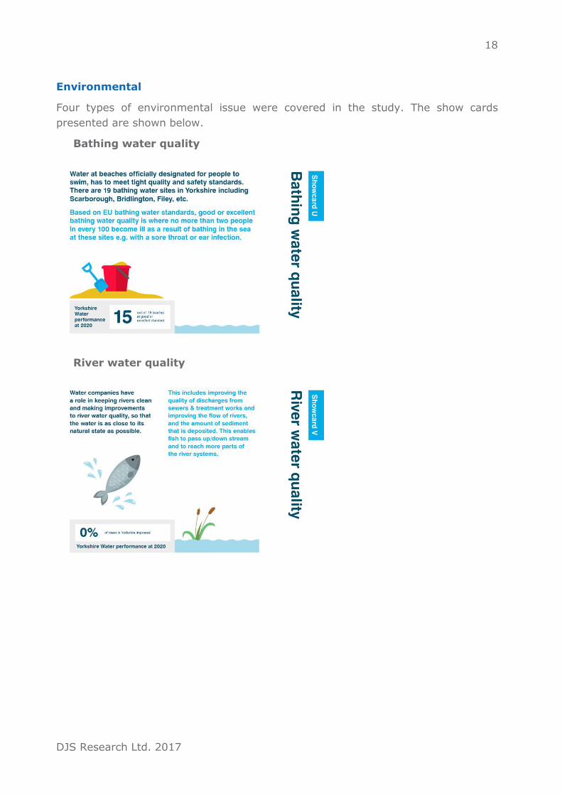
Environmental

Four types of environmental issue were covered in the study. The show cards


Bathing water quality

River water quality

19


Pollution incidents

Land conserved or improved by Yorkshire Water

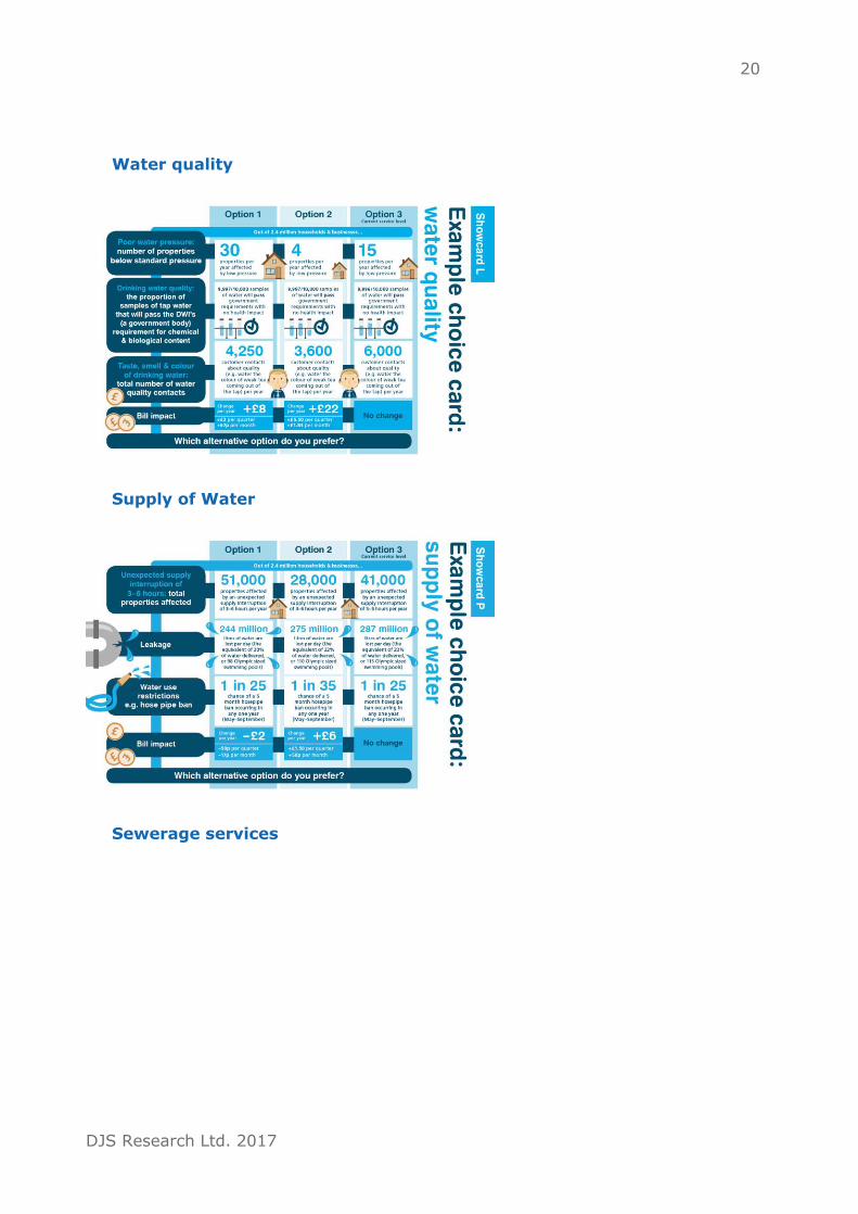
Choice experiment examples

Examples of the choice experiment grids presented to respondents to make their

stated preference choices against each of the service level areas, are shown below.

The only difference in the choice experiment examples shown to household and

business respondents was the option 1 and 2 values – where household customers

were shown a monetary value, business customers were shown a percentage change

figure.

20


Water quality

Supply of Water

Sewerage services

21


Environment

22


Whole package choice experiment

Respondents were also provided with a whole package choice experiment, with two

choices – either the top level of service per service level attribute, for a randomly

selected bill impact, or a no change option comprising of Yorkshire Water’s committed

service levels from 2020:

23


Appendix 2 – results and

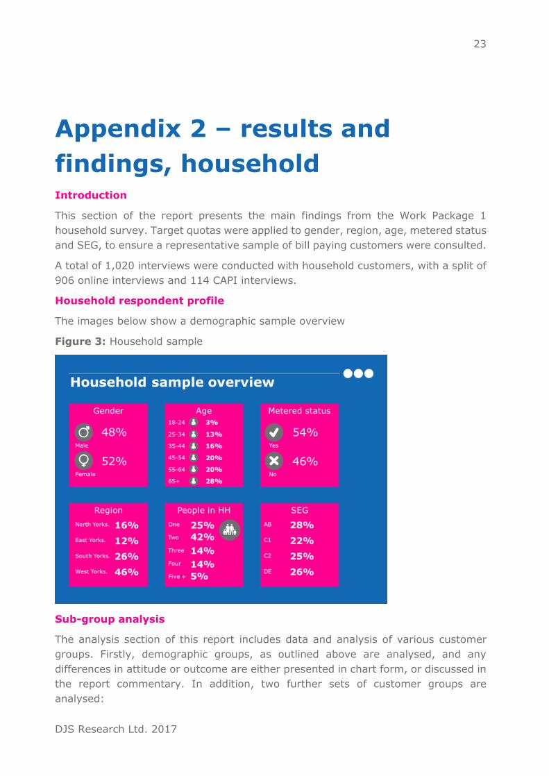
findings, household Introduction

This section of the report presents the main findings from the Work Package 1

household survey. Target quotas were applied to gender, region, age, metered status

and SEG, to ensure a representative sample of bill paying customers were consulted.

A total of 1,020 interviews were conducted with household customers, with a split of

906 online interviews and 114 CAPI interviews.

Household respondent profile

The images below show a demographic sample overview

Figure 3: Household sample

Sub-group analysis

The analysis section of this report includes data and analysis of various customer

groups. Firstly, demographic groups, as outlined above are analysed, and any

differences in attitude or outcome are either presented in chart form, or discussed in

the report commentary. In addition, two further sets of customer groups are

analysed:

24


• Customers in vulnerable circumstances vs. customers not in vulnerable

circumstances

• Customers who have had service experiences/outages in the past three years

vs. customers who haven’t experienced service experiences/outages in the

past three years

The next two sections discuss the make-up of the variables outlined above.

Customers in vulnerable circumstances

In order to identify customers who might find themselves in vulnerable circumstances

a number of questions were asked to respondents. Firstly, customers were asked to

rate the extent to which they agreed with three statements relating to the

affordability of water bills. Two statements dealt with concerns about paying water

bills (“I worry about not being able to afford my water bill” and, “I already can’t afford

my water bill”), and one statement concerned not thinking too much about water

bills (“I don’t really think about my water bill it’s just something I have to pay”)

Figure 4: Water bill affordability – household

Base: all household respondents, excluding don’t knows (as shown)

In the first iteration of the customers in vulnerable circumstances variable, customers

who strongly or slightly agreed with either of the top two sentiments were classed as

‘bill vulnerable’. However, as the analysis progressed, it became clear that the

definitions of vulnerability were too broad as to be useful, so a secondary analysis of

customers who agreed strongly with either of the top two sentiments was

undertaken.

25


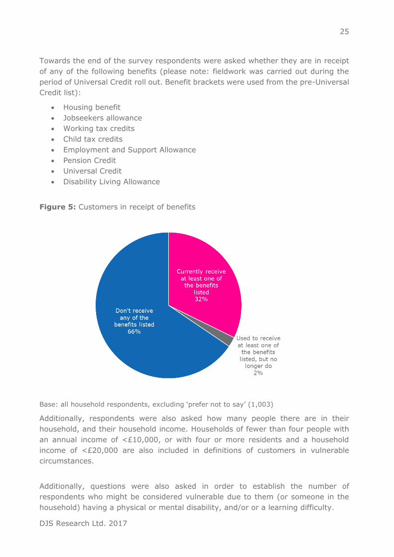
Towards the end of the survey respondents were asked whether they are in receipt

of any of the following benefits (please note: fieldwork was carried out during the

period of Universal Credit roll out. Benefit brackets were used from the pre-Universal

Credit list):

• Housing benefit

• Jobseekers allowance

• Working tax credits

• Child tax credits

• Employment and Support Allowance

• Pension Credit

• Universal Credit

• Disability Living Allowance

Figure 5: Customers in receipt of benefits

Base: all household respondents, excluding ‘prefer not to say’ (1,003)

Additionally, respondents were also asked how many people there are in their

household, and their household income. Households of fewer than four people with

an annual income of <£10,000, or with four or more residents and a household

income of <£20,000 are also included in definitions of customers in vulnerable

circumstances.

Additionally, questions were also asked in order to establish the number of

respondents who might be considered vulnerable due to them (or someone in the

household) having a physical or mental disability, and/or or a learning difficulty.

26


Figure 6: Households with someone registered disabled, or suffering from a severe

medical condition

Base: all household respondents, excluding ‘prefer not to say’ (1,014)

Of the 27% of customers who report someone in their household having a current or

historic disability or severe medical condition, 25.3% report the disability affecting

the way in which water is used/consumed (6.8% of the total).

A separate question asked of respondents in an effort to be able to classify

vulnerability was whether English is spoken as a first language, or not. Overall, only

21 (2%) interviews with respondents where English is not their 1st language were

recorded – meaning there isn’t a sufficient base of responses to include as a separate

(robust) definition of vulnerability due to language.

Based on the possible indicators of vulnerability discussed, four definitions have been

created, and are used for additional analysis later in the report:

• Possible vulnerability:

o respondents who agree, strongly or slightly, with either of the two bill

struggle statements, and/or;

o report being in receipt of benefits, and/or;

o report someone in the household having a disability and/or a learning

difficulty, and/or;

o live in a household of <4 people and have an annual household income

of <£10,000, or live in a household of 4+ people and have an annual

household income of <£20,000

27


This definition of potential vulnerability resulted in 54.8% of the sample being

flagged. Based on this large proportion, it was felt that a ‘stricter’ definition of

vulnerability was required in order to truly understand whether any differences in

attitude or WTP exist between customers in different circumstances. Therefore, a

second definition of vulnerability was created:

• Focussed vulnerability:

o respondents who agree strongly with either of the two bill struggle

statements, and or;

o respondents who receive help to pay their water bill, and/or;

o report someone in the household having a disability that impacts on the

way water is used/consumed

This more focussed definition resulted in 24.5% of the sample being flagged as

vulnerable.

In addition to these two definitions of vulnerability, 2 further definitions were created

and analysed in order to provide data comparability across Work Packages:

• Financially vulnerable:

o respondents who agree, strongly or slightly, with either of the two bill

struggle statements; and/or;

o Receive(d) help to pay a bill, and/or;

o Receive(d) benefits, and/or;

o live in a household of <4 people and have an annual household income

of <£10,000, or live in a household of 4+ people and have an annual

household income of <£20,000

• Health vulnerable:

o respondents aged 75+, and/or;

o respondents who report someone in the household having a disability

▪ Note: within the sample, there are no incidences of customers

age 75+ who don’t also report a disability

The financially vulnerable definition covers 41.7% of the sample, and the health

vulnerable definition covers 26.9% of the definition.

Service experiences

In order to include an additional layer of understanding to respondent reactions in

the stated preference exercises, respondents were asked whether they had ever

experienced any of the following water related service experiences whilst living in

Yorkshire. The chart overleaf shows the proportion of respondents reporting having

experienced each issue.

28


Figure 7: Service experiences - household

Base: all household respondents excluding don’t know per issue (as shown)

The 17% of respondents who said they had experienced smells from sewers or

sewage treatment works in the past three years were asked a follow up question

about where they experience the issue. Of those respondents, 46 (28%) said they’d

experienced the smells only at their property, and 26 (16%) said they’d experienced

smells caused by sewers/sewage treatment works both at their property and when

out. The remainder (56%) either couldn’t remember where they’d experienced the

smells, or had only experienced them when passing near a sewer/sewage treatment

works.

Overall, 209 (21%) have never experienced any of the incidents listed, and 369

(36%) have not experienced any of the incidents listed in the past 3 years. In the

past 12 months, 394 (39%) have experienced at least one of the incidents listed.

Attitudinal statements

The household surveys included a set of five attitudinal statements for use in

evaluating the impact of attitudes on water service values. The attitudinal statements

are controlled for as covariates within the modelling – used to estimate the

contribution of non-use values to a customer’s WTP.

This section outlines the overall response to these attitudinal statements at a total

level:

29


Figure 8: Attitudinal statements

Protecting Yorkshire’s land and water environments such as lakes, rivers, bathing

waters, woodlands, and grasslands is really important to me, because…

Base: all household respondents, excluding don’t know responses (as shown)

Due to high levels of agreement across all statements, further analysis using these

statements is based on a ‘strongly agree’ vs. the rest basis.

Analysis and results

This section of the report contains analysis of the household Willingness to Pay (WTP),

with a broad structure of the findings outlined as follows:

• Examination of the preference for the status quo

• Economic modelling results

• The final/preferred WTP table for each of the 4 CE blocks

• Results of the full-package CE

• Analysis of sub-group results

• Use and Non-Use values

• The validity of the outcomes

30


Preference for the status quo

The tables below summarise the choice behaviour observed within the household

customer samples across the four service area blocks:

Table 9: Choice frequencies for household samples

Status quo Alternative 1 Alternative 2





Table 10: Proportion of serial status quo choices and bill reduction option choices

Always choose

status quo

Always choose

bill increases

Always choose

bill reductions





Table 9 shows that the status quo is selected at least half of the time across the four

service areas - revealing a very high level of choice of the status quo option within

each of the service area blocks. There is some level of trading with the alternative

hypothetical options noted, particularly in the environmental service block.

Table 10, meanwhile, shows the percentage of respondents who always select the

status quo (or increases or decreases) – showing that around a third of respondents

consistently choose the status quo when given multiple choices. The remainder of

respondents in Table 10 select different options across the CE sets within the blocks.

Economic modelling results

Block 1 - Water Quality

31


After extensive analysis of the data, three models were considered to describe the

choice data obtained from the domestic customers. The first was a simple Conditional

Logit model, while the other two were the Random Parameter Logit model and the

Generalised Mixed Logit model.

For the Water Quality choice set based on CE1, the Random Parameter Logit model

performed best in terms of goodness-of-fit to the data with a Pseudo 𝑅2, = 0.20

(compared with 0.16 for the Generalised Mixed Logit model, and 0.17 for the

Conditional Logit model). In the Random Parameter Logit model, tastes were

assumed to be normally distributed with respect to the service measures (poor water

pressure, drinking water quality and taste, smell and colour of drinking water); but

the bill coefficient was assumed to be fixed, as was the status quo coefficient.

Table 11 below reports the results of all three models. The positive signs on the

coefficients of the Water Quality in the models conformed to prior expectations, i.e.

as the service level increases, so the probability of choice increases. All of the

coefficients were highly statistically significant at the 99% level. The coefficient for

the status quo choice is positive and statistically significant suggesting that the

presence of the status quo option was a significant factor in respondent choices (as

noted earlier, a high level of preference for the status quo option exists).

Table 11: Models of Water Quality choice data

Conditional Logit Random Parameter

Logit Generalised Mixed

Logit

Pseudo 𝑅2 0.17 Pseudo 𝑅2 0.20 Pseudo 𝑅2 0.16

Coefficient Prob.|z|>Z Coefficient Prob.|z|>Z Coefficient Prob.|z|>Z

Poor water pressure: number of properties below

standard pressure

0.19063 0.0000 0.13645 0.0000 0.177546 0.0000

Drinking water

quality: the proportion of samples of tap water that will pass the DWI’s (a

government body) requirement for chemical

0.16774 0.0000 0.185962 0.0000 0.196532 0.0000

32


& biological content

Taste, smell & colour of drinking water: total number of water

quality contacts

0.55537 0.0000 0.44492 0.0000 0.4866 0.0000

Bill impact -0.13444 0.0000 -0.11507 0.0418 -0.15422 0.0000

Status quo 0.60757 0.0000 0.752369 0.0000 0.58756 0.0000

The marginal WTP for a service level change in each service measure are presented

in Table 12. Based on the Conditional Logit model, domestic customers were prepared

to pay on average £0.66 more on their bill for each increase in drinking water quality

service level. Table 12 also reports the 95% confidence intervals associated with

marginal WTP for all three models.

The Random Parameter Logit model, which is linear, suggests that the average

domestic customer is willing to pay an additional £2.07 for a level increase in taste,

smell and colour of drinking water.

Table 12: WTP results for Water Quality choice data

Conditional Logit Random

Parameter Logit

Generalised Mixed

Logit

Marginal WTP

95% LL

95%UL Marginal

WTP

95% LL

95%UL Marginal

WTP

95% LL

95%UL

Poor water pressure

£0.75 £0.56 £0.93 £0.64 £0.48 £0.79 £0.74 £0.55 £0.92

Drinking water quality

£0.66 £0.47 £0.84 £0.87 £0.72 £1.02 £0.82 £0.60 £1.03

Taste, smell and colour of drinking

water

£2.17 £1.97 £2.37 £2.07 £1.74 £2.41 £2.02 £1.89 £2.14

All three of the models reported above assume a linear relationship between WTP

and the level of service they receive. However as previously suggested, WTP and

WTA tend not to be symmetrical. Such a non-linear utility function can be modelled

with a non-linear function; but an alternative is to model the non-linear relationship

through a piecewise regression model (i.e. fixed effects model). A non-linear utility

change model or fixed effects model is therefore used to assess whether a non-linear

relationship holds for service improvements and service reductions.

The non-linear utility change model, or fixed effects model, was estimated using each

of the three models used above. While the Generalised Mixed Logit and Random

33


Parameter Logit models provide a better fit with the data they do not provide

statistically significant coefficient values for a number of the service measure effects.

Given that the purpose of this exercise is to estimate customer WTP for improvements

in service measure levels it was decided to base the following discussion on the

Conditional Logit Model (table 13), where most coefficient values are significant and

capable of meaningful interpretation.

In this model most coefficients change monotonically: for example, drinking water

quality(L-1) < drinking water quality(L+1) < drinking water quality(L+2) < drinking

water quality(L+3).

Table 13: Non-Linear Conditional Logit model for water quality

Pseudo 𝑹𝟐 0.16

Observations = 9180

Coefficient Prob.|z|>Z Marginal WTP 95% LL 95%UL

Poor water pressure (L-2)

-0.62899 0.000 -£2.25 -£2.70 -£1.79


-0.38497 0.000 -£1.37 -£1.52 -£1.23

Poor water pressure (L+1)

0.13327 0.007 £0.48 £0.32 £0.63

Poor water

pressure (L+2) 0.22959 0.007 £0.82 £0.50 £1.14


0.29565 0.016 £1.05 £0.76 £1.81

Drinking water quality (L-2)

-0.52912 0.000 -£1.89 -£2.82 -£0.96


-0.31188 0.000 -£1.11 -£1.42 -£0.80

Drinking water quality (L+1)

0.13701 0.000 £0.49 £0.34 £0.64


0.4654 0.001 £1.66 £1.37 £1.95


0.5986 0.005 £2.15 £1.74 £2.75

Taste, smell and colour of drinking water (L-2)

-0.94947 0.000 -£3.39 -£4.05 -£2.74


-0.41606 0.000 -£1.49 -£1.78 -£1.19

Taste, smell and colour of drinking water (L+1)

0.58444 0.000 £2.09 £1.42 £2.75

34



1.04639 0.000 £3.74 £2.79 £4.68


1.2236 0.000 £4.40 £3.54 £5.27

Bill impact -0.09603 0.000

The results of the fixed effects model indicate that the average domestic customer

would be prepared to pay a +£1.66 increase on their water bill to increase drinking

water quality level from the status quo to level +2. The average customer would be

willing to accept a decrease in taste, smell and colour of drinking water to level -1

for a bill reduction of -£1.49 per year.

Overall, the fixed effect model for water quality indicates that there is diminishing

marginal utility for improvements in some service measure levels; and also,

asymmetry between WTP and WTA. This suggests the non-linear approach is superior

to the linear assumptions of the previous models.

Block 2 – Supply of Water

Again, the 3 models were applied to the data relating to CE2, Supply of Water.

For the Supply of Water choice set based on CE2, the Random Parameter Logit model

performed best in terms of goodness-of-fit to the data with a Pseudo 𝑅2, = 0.27


Conditional Logit Model). In the Random Parameter Logit Model, tastes were assumed

to be normally distributed with respect to the service measures (unexpected supply

interruption, leakage and water use restrictions); but the bill coefficient was assumed

to be fixed, as was the status quo coefficient.

Table 14 reports the results of all three models. The positive signs on the coefficients

of the Supply of Water in the models conformed to prior expectations, i.e. as the

service level increases, so the probability of choice increases. All of the coefficients

were statistically significant at the 5% level. The coefficient for the status quo choice

is positive and statistically significant suggesting that the presence of the status quo

option was a significant factor in respondent choices (as noted earlier, a high level of

preference for the status quo option exists).

Table 14: Models of Supply of Water choice data


Logit

Generalised Mixed

Logit



35



properties affected

0.42834 0.0000 0.39569 0.0000 0.456554 0.0000

Leakage 0.40739 0.0000 0.454667 0.0000 0.485652 0.0000

Water use restrictions e.g. hose pipe ban

0.14506 0.0000 0.17344 0.0338 0.123357 0.0000

Bill impact -0.26257 0.0000 -0.25292 0.02825 -0.26684 0.0000

Status quo 0.28764 0.0155 0.25963 0.0006 0.33237 0.00012

The marginal WTP for a service level change in each service measure is presented in

Table 15. Based on the Conditional Logit model, domestic customers were prepared

to pay on average +£0.81 more on their bill for each increase in unexpected supply

interruption service level. Table 15 also reports the 95% confidence intervals

associated with marginal WTP for all three models.

The Random Parameter Logit model suggests that the average domestic customer is

willing to pay an additional +£0.35 for a level increase in water use restrictions.

Table 15: WTP results for Supply of Water choice data


Logit

Generalised Mixed

Logit

Marginal WTP

95% LL

95%UL Marginal

WTP

95% LL

95%UL Marginal

WTP

95% LL

95%UL

Unexpected supply interruption

£0.81 £0.73 £0.90 £0.72 £0.64 £0.80 £0.80 £0.70 £0.90

Leakage £0.77 £0.69 £0.86 £0.83 £0.74 £0.91 £0.85 £0.78 £0.92


£0.31 £0.21 £0.40 £0.35 £0.20 £0.50 £0.24 £0.18 £0.29

All three of the models reported above imply that there is a linear relationship

between WTP and the level of service they receive. However, the alternative is to

model the non-linear relationship through a piecewise regression model (i.e. a fixed

effects model). A non-linear utility change model or fixed effects model is therefore

used to assess whether a non-linear relationship holds for service improvements and

service reductions.

36


The non-linear utility change model is again based on the Conditional Logit model

(see Table 16), where most coefficient values are significant and capable of

meaningful interpretation.

37


Table 16: Non-Linear Conditional Logit model for Supply of Water


Observations = 9180


Unexpected

supply interruption (L-2)

-0.79613 0.000 -£1.48 -£1.81 -£1.16

Unexpected supply

interruption (L-1)

-0.44171 0.000 -£0.82 -£1.12 -£0.53

Unexpected supply

interruption

(L+1)

0.1055 0.020 £0.20 £0.12 £0.27


(L+2)

0.32734 0.000 £0.61 £0.53 £0.69

Unexpected supply

interruption (L+3)

0.41326 0.000 £0.77 £0.65 £0.89

Leakage (L-2) -0.86924 0.000 -£1.62 -£1.99 -£1.25

Leakage (L-1) -0.5833 0.000 -£1.09 -£1.41 -£0.76

Leakage (L+1) 0.23618 0.063 £0.44 £0.21 £0.67

Leakage (L+2) 0.38712 0.056 £0.72 £0.12 £1.32

Leakage (L+3) 0.4452 0.065 £0.83 £0.24 £1.42

Water use restrictions (L-2)

-0.27771 0.002 -£0.52 -£0.85 -£0.19

Water use restrictions (L-1)

-0.26775 0.001 -£0.50 -£0.80 -£0.19

Water use

restrictions (L+1)

0.1389 0.009 £0.26 £0.15 £0.37

Water use

restrictions (L+2)

0.14071 0.035 £0.26 £0.18 £0.35


(L+3)

0.1536 0.042 £0.29 £0.20 £0.38

Bill impact -0.12805 0.000

38



would be prepared to pay a +£0.72 increase on their water bill to increase leakage

level from the status quo to level +2. The average customer would be willing to

accept a decrease in leakage to level -1 for a bill reduction of -£1.09 per year.

Overall, the fixed effect model for Supply of Water indicates that there is diminishing


asymmetry between WTP for improvements in service levels and WTA (compensation

or bill reductions) for a lower level of service. This suggests the non-linear approach

is superior to the linear assumptions of the previous models.

Block 3 – Sewerage Services

Again, the 3 models were applied to the data relating to CE3, sewerage services.

For the sewerage services choice set based on CE3, the Random Parameter Logit

model performed best in terms of goodness-of-fit to the data with a Pseudo 𝑅2, =

0.19 (compared with 0.17 for the Generalised Mixed Logit model, and 0.17for the

Conditional Logit model). In the RPL model, tastes were assumed to be normally

distributed with respect to the service measures s (sewer flooding inside properties,

sewer flooding outside properties and Properties subjected to chronic (seasonal)

unbearable smells from sewers & treatment works); but the bill coefficient was

assumed to be fixed, as was the status quo coefficient.


of the sewerage services in the models conformed to prior expectations, i.e. as the




option was a significant factor in respondent choice.

39


Table 17: Models of Sewerage Services choice data



Logit



Sewer flooding inside properties:

number of incidents

per year

0.47757 0.0000 0.53403 0.0062 0.512367 0.0000

Sewer

flooding outside properties: number of incidents per year

0.29141 0.0000 0.29457 0.0241 0.266534 0.0000

Properties subjected to chronic (seasonal)

unbearable smells from sewers &

treatment works: complaints

to Yorkshire Water per year

0.299857 0.0000 0.27929 0.0219 0.313222 0.0000

Bill impact -0.24351 0.0000 -0.28759 0.0003 -0.26598 0.0000

Status quo 0.28895 0.014 0.20028 0.06025 0.299896 0.009506



to pay on average +£0.92 more on their bill for each increase in sewer flooding inside

properties: number of incidents per year service level. Table 18 also reports the 95%

confidence intervals associated with marginal WTP for all three models.

The Random Parameter Logit model suggests that the average domestic customer is

willing to pay an additional +£0.52 for a level increase in properties subjected to

chronic (seasonal) unbearable smells from sewers & treatment works.

40


Table 18: WTP results for Sewerage Services choice data

Conditional

Logit Random Parameter


Logit

Marginal

WTP

95%

LL 95%UL

Marginal

WTP

95%

LL 95%UL

Marginal

WTP

95%

LL 95%UL

Sewer flooding inside properties:

number of incidents per year

£0.92 £0.83 £1.01 £0.99 £0.71 £1.28 £0.97 £0.89 £1.05

Sewer

flooding outside properties: number of incidents per year

£0.56 £0.48 £0.65 £0.55 £0.43 £0.66 £0.50 £4.39 -£3.38


smells from sewers & treatment

works: complaints


£0.58 £0.46 £0.69 £0.52 £0.46 £0.58 £0.59 £0.52 £0.66






service reductions.

The non-linear utility change model is again based on the Conditional Logit

Conditional Logit model (see Table 19), where most coefficient values are significant

and capable of meaningful interpretation.

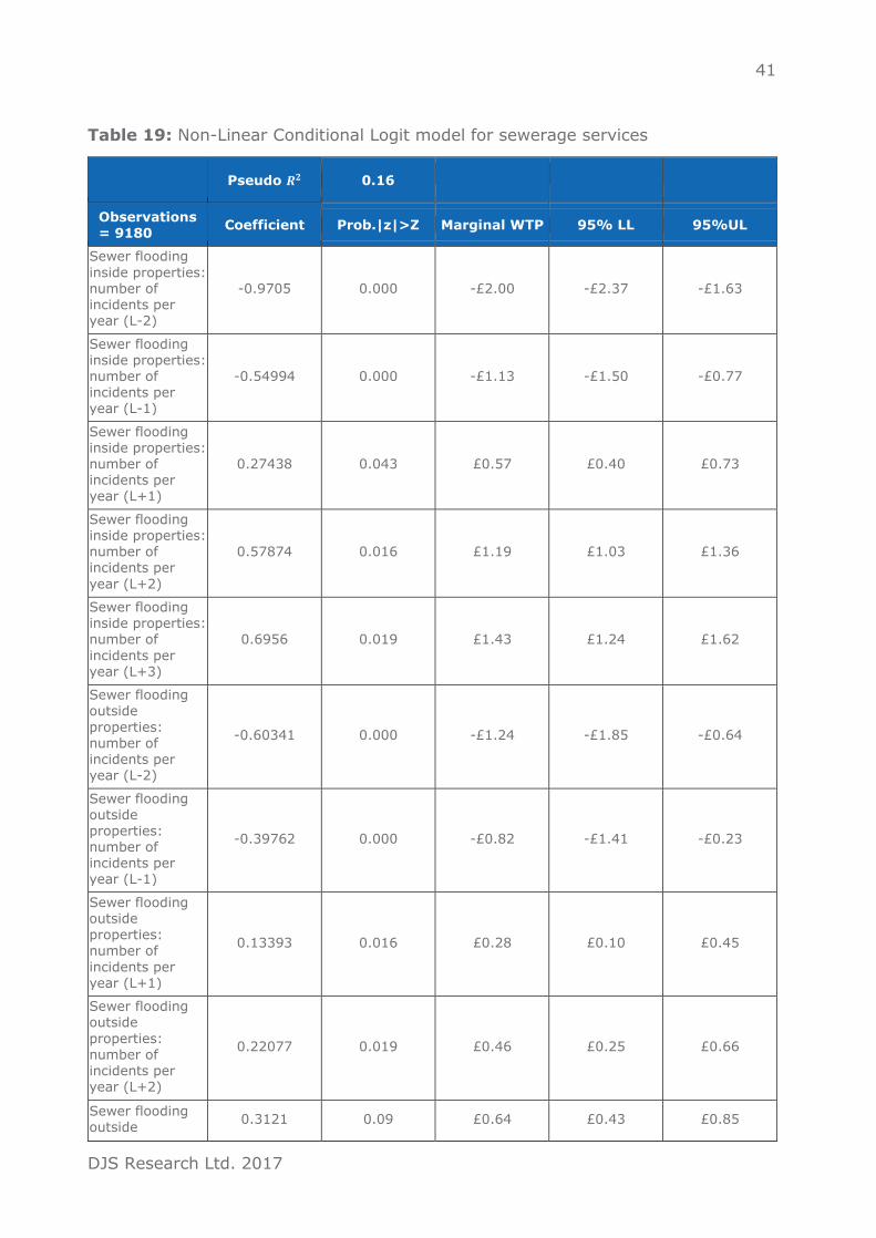
41


Table 19: Non-Linear Conditional Logit model for sewerage services


Observations = 9180


Sewer flooding

inside properties: number of incidents per year (L-2)

-0.9705 0.000 -£2.00 -£2.37 -£1.63

Sewer flooding inside properties: number of

incidents per year (L-1)

-0.54994 0.000 -£1.13 -£1.50 -£0.77

Sewer flooding inside properties: number of incidents per year (L+1)

0.27438 0.043 £0.57 £0.40 £0.73


year (L+2)

0.57874 0.016 £1.19 £1.03 £1.36


incidents per year (L+3)

0.6956 0.019 £1.43 £1.24 £1.62

Sewer flooding outside

properties: number of incidents per year (L-2)

-0.60341 0.000 -£1.24 -£1.85 -£0.64

Sewer flooding outside properties: number of incidents per year (L-1)

-0.39762 0.000 -£0.82 -£1.41 -£0.23


properties: number of

incidents per year (L+1)

0.13393 0.016 £0.28 £0.10 £0.45


properties: number of incidents per year (L+2)

0.22077 0.019 £0.46 £0.25 £0.66


0.3121 0.09 £0.64 £0.43 £0.85

42


properties: number of incidents per year (L+3)


smells from sewers & treatment works: complaints to Yorkshire Water per year (L-2)

-0.43751 0.000 -£0.90 -£1.29 -£0.51


smells from sewers & treatment works: complaints to Yorkshire Water per year (L-1)

-0.10082 0.028 -£0.21 -£0.40 -£0.01


unbearable

smells from sewers & treatment works: complaints to Yorkshire Water per year (L+1)

0.19354 0.022 £0.40 £0.27 £0.52


unbearable smells from sewers & treatment works: complaints to Yorkshire Water

per year (L+2)

0.29183 0.003 £0.60 £0.34 £0.86

Properties subjected to chronic

(seasonal) unbearable smells from sewers & treatment works: complaints to Yorkshire Water

per year (L+3)

0.3220 0.006 £0.66 £0.45 £0.87

43


Bill impact -0.1506 0.000


would be prepared to pay a +£1.19 increase on their water bill to increase sewer

flooding inside properties level from the status quo to level +2. The average customer

would be willing to accept a decrease in properties subject to chronic smells to level

-1 for a bill reduction of -£0.21 per year.

Overall, the fixed effect model for sewerage services indicates that there is

diminishing marginal utility for improvements in some service measure levels; and

also, asymmetry between WTP for improvements in service levels and WTA

(compensation or bill reductions) for a lower level of service. This suggests the non-

linear approach is superior to the linear assumptions of the previous models.

Block 4 – Environment

For the environment choice set based on CE4, the Conditional Logit model performed

best in terms of goodness-of-fit to the data with a Pseudo 𝑅2 = 0.25 (compared with

0.22 for the Generalised Mixed Logit model, and 0.19 for the Random Parameter

Logit model). In the Random Parameter Logit model, tastes were assumed to be

normally distributed with respect to the service measures s (number of bathing

beaches meeting ‘Good’ or ‘Excellent’ standard, length of rivers in Yorkshire

improved, category 3 pollution incident, and area of land conserved or improved by

Yorkshire Water); but the bill coefficient was assumed to be fixed, as was the status

quo coefficient.


of the environment in the models conformed to prior expectations, i.e. as the service

level increases, so the probability of choice increases. All of the coefficients were

statistically significant at the 5% level. The coefficient for the status quo choice is

positive and statistically significant suggesting that the presence of the status quo


44


Table 20: Models of Environment choice data



Logit



Number of bathing beaches meeting

‘Good’ or ‘Excellent’

standard

0.14935 0.0000 0.131222 0.0000 0.152236 0.0000

Length of

rivers in Yorkshire improved (%)

0.40956 0.0000 0.44395 0.0013 0.412356 0.0000

Category 3 pollution incident: a minor incident

that has a minimal impact on the

quality of water in the area

0.20553 0.0000 0.21825 0.0000 0.239562 0.0000

Area of land conserved or

improved by Yorkshire Water

0.20544 0.0000 0.20951 0.0365 0.198956 0.0000

Bill impact

-0.19872 0.0000 -0.30226 0.0018 -0.24224 0.0000

Status quo

0.13399 0.0000 0.1702 0.00512 0.165459 0.0000



to pay on average +£1.11 more on their bill for each increase in the length of rivers

in Yorkshire improved service level. Table 21 also reports the 95% confidence

intervals associated with marginal WTP for all three models.

45


Table 21: WTP results for environment choice data

Conditional

Logit Random Parameter


Logit

Marginal

WTP

95%

LL 95%UL

Marginal

WTP

95%

LL 95%UL

Marginal

WTP

95%

LL 95%UL


‘Good’ or ‘Excellent’ standard

£0.40 £0.29 £0.34 £0.26 £0.43 £0.40 £0.29 £0.51 £0.40

Length of


£1.11 £0.98 £1.16 £1.02 £1.31 £1.08 £0.98 £1.18 £1.08

Category 3 pollution incident: a minor incident that has a minimal

impact on the quality of water in the area

£0.56 £0.44 £0.57 £0.46 £0.68 £0.63 £0.49 £0.76 £0.63

Area of land conserved or improved by

Yorkshire Water

£0.56 £0.45 £0.55 £0.40 £0.70 £0.52 £0.44 £0.61 £0.52






service reductions.




46


Table 22: Non-Linear Conditional Logit model for environment


Observations = 9180


Number of

bathing beaches meeting ‘Good’ or ‘Excellent’ standard (L-2)

-0.62446 0.000 -£1.64 -£2.13 -£1.15

Number of bathing beaches meeting ‘Good’

or ‘Excellent’ standard (L-1)

-0.34585 0.001 -£0.91 -£1.35 -£0.47

Number of bathing beaches meeting ‘Good’ or ‘Excellent’ standard (L+1)

0.12209 0.009 £0.32 £0.20 £0.45


standard (L+2)

0.1816 0.030 £0.48 £0.26 £0.69


or ‘Excellent’ standard (L+3)

0.1865 0.029 £0.49 £0.25 £0.70

Length of rivers in Yorkshire

improved (%) (L-2)

-0.55843 0.000 -£1.47 -£2.08 -£0.86


improved (%) (L-1)

-0.3128 0.000 -£0.82 -£1.05 -£0.59


improved (%) (L+1)

0.31487 0.044 £0.83 £0.64 £1.01

Length of rivers

in Yorkshire

improved (%) (L+2)

0.4339 0.040 £1.14 £0.96 £1.32

Length of rivers

in Yorkshire improved (%) (L+3)

0.5132 0.026 £1.35 £1.17 £1.53

Category 3

pollution incident: a minor incident that has a minimal impact

-0.59701 0.000 -£1.57 -£1.99 -£1.15

47


on the quality of water in the area (L-2)

Category 3 pollution incident: a minor incident that has a minimal impact on the quality of

water in the area (L-1)

-0.16218 0.052 -£0.43 -£0.70 -£0.15

Category 3 pollution

incident: a minor incident that has

a minimal impact on the quality of water in the area (L+1)

0.12715 0.078 £0.33 £0.12 £0.55

Category 3 pollution incident: a minor incident that has a minimal impact

on the quality of water in the area (L+2)

0.22881 0.013 £0.60 £0.44 £0.77

Category 3 pollution incident: a minor incident that has

a minimal impact on the quality of water in the area

(L+3)

0.3123 0.023 £0.82 £0.64 £1.00


Yorkshire Water (L-2)

-0.54773 0.000 -£1.44 -£1.90 -£0.98


improved by Yorkshire Water (L-1)

-0.21405 0.000 -£0.56 -£0.85 -£0.28

Area of land

conserved or improved by Yorkshire Water (L+1)

0.14724 0.060 £0.39 £0.09 £0.68

Area of land conserved or improved by Yorkshire Water (L+2)

0.20249 0.026 £0.53 £0.38 £0.68


0.2220 0.033 £0.58 £0.42 £0.74

48


Yorkshire Water (L+3)

Bill impact -0.10394 0.000


would be prepared to pay a +£1.14 increase on their water bill to increase Length of

rivers in Yorkshire improved (%) level from the status quo to level +2. The average

customer would be willing to accept a decrease in area of land conserved or improved

by Yorkshire Water to level -1 for a bill reduction of -£0.56 per year.

Overall, the fixed effect model for environment indicates that there is diminishing





Willingness to Pay estimates

The final WTP and WTA based on the non-linear model estimates are summarised in

Table 23. In almost all of the service level areas considered, the level of WTA is

greater than the level of WTP for the greatest service decrease or increase.

49


Table 23: WTP and WTA estimates – all service levels

Service area

Service level attribute

Willingness to Pay

Reduction

in service

Improvement in service

-1 +1 +2 +3

Water quality


number of properties below standard pressure

-£1.37 £0.48 £0.82 £1.05

Drinking water quality:

the proportion of samples of tap water that will pass

the DWI’s (a government body) requirement for chemical & biological content

-£1.11 £0.49 £1.66 £2.15

Taste, smell & colour of drinking water: total number of water quality contacts

-£1.49 £2.09 £3.74 £4.40

Supply of Water

Unexpected supply interruption of 3–6 hours: total properties affected

-£0.82 £0.20 £0.61 £0.77

Leakage -£1.09 £0.44 £0.72 £0.83


-£0.50 £0.26 £0.26 £0.29

Sewerage

services


incidents per year

-£1.13 £0.57 £1.19 £1.43

Sewer flooding outside properties: number of incidents per year

-£0.82 £0.28 £0.46 £0.64

Properties subjected to chronic (seasonal) unbearable smells from sewers & treatment

works: complaints to Yorkshire Water per year

-£0.21 £0.40 £0.60 £0.66

Environment

Number of bathing beaches meeting ‘Good’ or

‘Excellent’ standard

-£0.91 £0.32 £0.48 £0.49

Length of rivers in Yorkshire improved (%)

-£0.82 £0.83 £1.14 £1.35

Category 3 pollution incident: a minor incident that has a minimal impact on the quality of water in the area

-£0.43 £0.33 £0.60 £0.82

Area of land conserved or improved by Yorkshire Water

-£0.56 £0.39 £0.53 £0.58

50


Table 24: WTP and WTA estimates – online community panel

Service area

Service level attribute

Willingness to Pay

Reduction

in service


-1 +1 +2 +3

Water quality


number of properties below standard pressure

-£1.37

(-£1.19)

£0.48

(£0.80)

£0.82

(£1.02)

£1.05

(£1.67)

Drinking water quality: the proportion of samples

of tap water that will pass the DWI’s (a government body) requirement for chemical & biological content

-£1.11

(-£0.96)

£0.49

(£0.67)

£1.66 (£1.22)

£2.15

(£2.70)

Taste, smell & colour of drinking water: total number of water quality contacts

-£1.49

(-£1.35)

£2.09

(£1.89)

£3.74

(£3.51)

£4.40

(£4.62)

Supply of water

Unexpected supply interruption of 3–6 hours: total properties affected

-£0.82

(-£0.50)

£0.20

(£0.48)

£0.61

(£0.91)

£0.77

(£1.03)

Leakage -£1.09

(-£0.80)

£0.44

(£0.39)

£0.72

(£0.86)

£0.83

(£1.12)

Water use restrictions e.g.

hose pipe ban

-£0.50

(-£0.27)

£0.26

(£0.32)

£0.26

(£0.39)

£0.29

(£0.48)

Sewerage services

Sewer flooding inside properties: number of incidents per year

-£1.13

(-£0.83)

£0.57

(£0.69)

£1.19

(£1.18)

£1.43

(£1.73)


properties: number of incidents per year

-£0.82

(-£0.68)

£0.28

(£0.32)

£0.46

(£0.66)

£0.64

(£0.87)

Properties subjected to chronic (seasonal) unbearable smells from sewers & treatment works: complaints to

Yorkshire Water per year

-£0.21

(-£0.31)

£0.40

(£0.45)

£0.60

(£0.63)

£0.68

(£0.81)

Environment Number of bathing beaches meeting ‘Good’ or ‘Excellent’ standard

-£0.91

(-£1.22)

£0.32

(£0.68)

£0.48

(£1.37)

£0.49

(£1.66)

51



-£0.82

(-£0.63)

£0.83

(£0.71)

£1.14

(£1.28)

£1.35

(£1.82)


-£0.43

(-£0.99)

£0.33

(£0.65)

£0.60

(£0.98)

£0.82

(£1.43)


-£0.56

(-£1.13)

£0.39

(£0.42)

£0.53

(£0.91)

£0.58

(£1.31)

In general, the values from the online community WTP analysis are well matched

between the online community sample and the main stage survey sample; although

some individual levels have some large differences (for example – over £1 between

the acceptance for a decline L-2 in water taste & smell); most levels show little

change and are directionally comparable. The online community sample is skewed

slightly towards older age groups, and there is a higher proportion of females in the

sample than in the nat. rep main stage sample.

Full package CE

In the final choice experiment, CE5, respondents were presented with the full

package of 13 service levels shown at highest levels of service (L+3) at a range of

bill impacts for the total package (£30, £50, £65, £80, £100, £120).

The level of acceptance declines at each increased water bill impact. In each case,

the status quo is preferred to the alternative scenario.

Table 25: CE5 choice by scenario at each bill impact

Alternative scenario (L+3) Status quo – no bill impact

£30 40.9% 59.1%

£50 34.8% 65.2%

£65 34.0% 66.0%

£80 32.5% 67.5%

£100 31.4% 68.6%

£120 27.0% 73.0%

52


Variation in estimated WTP by socio-economic, and demographic

characteristics

The choice models investigated provide the ability to estimate WTP for individual

attributes at the level of individual respondents. This allows us to investigate how

respondent WTP varies across the household samples according to a range of

characteristics.

We have explored the variation in household WTP against the following classifications

of factors:

• Age: Under 45 vs. 45+

• Gender: Male vs. Female

• Household size: Number of people in the household

• Metered status: Metered vs. Unmetered

• SEG: ABC1 vs. C2DE

• Region

• Vulnerability: Not vulnerable vs. Possible vulnerability

• Vulnerability: Not focussed vulnerability vs. Focussed vulnerability

• Vulnerability: Not financially vulnerable vs. Financially vulnerable

• Vulnerability: Not health vulnerable vs. Health vulnerable

• Method of interview: Online vs. CAPI

• Service experiences

The following tables show only significant differences. Measures that show no data

show no significant difference in WTP values between comparative groups.

53


Table 26: Variation in estimated WTP by age

Service area

Service level attribute <45 +45

Water quality

Poor water pressure £0.93 £0.60


Taste smell and colour of drinking water

£2.16 £3.40

Supply of water


Leakage £0.65 £1.00


Sewerage services



£0.37 £0.91

Smell from sewers and treatment works

£0.71 £0.50

Environment

Bathing water quality £0.32 £0.53

River water quality

Pollution incidents

Land conserved or


£0.45 £0.69

WTP estimates by age show that younger customers (under 45) place a significantly

higher value on reducing the number of properties affected by poor water pressure,

and combating smells from sewers and sewage treatment works than customers who

are aged 45 and over. Older customers meanwhile place a significantly higher WTP

value on the taste, smell and colour of drinking water, reducing the incidence of

leakage, sewer flooding outside properties, river water quality and land conserved or

improved by Yorkshire Water. Overall, older customers are willing to pay more,

across a wider variety of service measures than younger customers.

54


Table 27: Variation in estimated WTP by Gender

Service area

Service level attribute Female Male

Water quality

Poor water pressure



Supply of water


Leakage


Sewerage services




Environment


River water quality

Pollution incidents £0.61 £0.51

Land conserved or improved by Yorkshire

Water

The only gender difference in WTP concerns pollution incidents, where females have

a higher WTP value than their male counterparts. Otherwise, no significant

differences are observed.

55


Table 28: Variation in estimated WTP by number of people in the home

Service area

Service level attribute 1 2 3 4+

Water quality

Poor water pressure £0.58 £0.78 £0.67 £0.94

Drinking water quality £0.55 £0.68 £0.71 £0.72


Supply of water


Leakage £0.72 £0.83 £0.85 £0.65


Sewerage services

Sewer flooding inside properties £0.78 £1.05 £0.91 £0.85


Smell from sewers and treatment

works £0.49 £0.61 £0.66 £0.57

Environment


River water quality

Pollution incidents £0.98 £1.21 £1.08 £1.10


Significant differences by size of household are noted for 6 service measures. The

most marked WTP differences are between the one person households and multiple

occupancy homes with the one person households having a consistently lower WTP

estimate across the six significantly different service measures.

56


Table 29: Variation in estimated WTP by metered status

Service area

Service level attribute Metered Unmetered

Water quality

Poor water pressure



£2.43 £3.08

Supply of water


Leakage


Sewerage services


£0.80 £1.02


£0.65 £0.50


Environment


River water quality

Pollution incidents

Land conserved or


Significant differences in WTP estimates only occur across three of the 13 service

measures. Metered customers place a higher WTP value on sewer flooding outside

properties, while unmetered customers would be willing to pay more for the taste

smell and colour of drinking water (although WTP estimates across both groups are

high) and sewer flooding inside properties.

57


Table 30: Variation in estimated WTP by SEG

Service area

Service level attribute ABC1 C2DE

Water

quality

Poor water pressure

Drinking water quality £0.81 £0.59


Supply of water

Unexpected supply

interruption £0.97 £0.74

Leakage £0.87 £0.70


Sewerage services


£1.16 £0.81


£0.69 £0.49

Smell from sewers and

treatment works £0.66 £0.53

Environment


River water quality £1.29 £1.00

Pollution incidents

Land conserved or


£0.66 £0.50

Unsurprisingly, higher SEG customers display a higher WTP propensity than lower

SEG customers. In particular, higher SEG customers’ WTP estimates are higher

across all three sewerage service measures. Interestingly, there is no difference in

WTP for the highest valued service measure; taste, smell and colour of drinking water

– suggesting that customers across both categories are equally unlikely to want to

compromise on this service area.

58


59


Table 31: Variation in estimated WTP by Region

Service area

Service level attribute East

Yorks.

North Yorks.

South Yorks.

West

Yorks.

Water quality

Poor water pressure £0.75 £0.81 £0.67 £0.78



Supply of water

Unexpected supply interruption £0.67 £0.90 £0.75 £0.85

Leakage


Sewerage services

Sewer flooding inside properties £1.06 £0.95 £0.84 £0.92



Environment


River water quality £1.24 £1.08 £1.13 £1.07

Pollution incidents


Water

Customers in South Yorkshire show the lowest WTP levels for poor water pressure

and sewer flooding inside properties. Meanwhile, customers in East Yorkshire have

the lowest WTP estimate for unexpected supply interruptions, but the highest for

river water quality and for inside sewer flooding.

60


61


Table 32: Variation in estimated WTP by possible vulnerability

Service area

Service level attribute Not possible vulnerability Possible vulnerability

Water quality




£2.37 £2.10

Supply of water


Leakage


Sewerage services




Environment


River water quality

Pollution incidents


Water

When looking at the broadest of the four vulnerable customer definitions few

significant differences emerge – with no differences apparent across the supply of

water, sewerage services or environment blocks. Where differences do appear, in the

water quality measures, non-vulnerable customers (by this definition) display a

higher WTP to reduce the chances of poor water pressure, and being affected by

water quality issues relating to the taste, smell and colour of drinking water.

62


63


Table 33: Variation in estimated WTP by focussed vulnerability

Service area

Service level attribute Not focussed vulnerability

Focussed vulnerability

Water quality




£2.29 £2.03

Supply of water


Leakage £0.81 £0.70


Sewerage services




Environment


River water quality

Pollution incidents


Water

When a more focussed definition of vulnerability is applied, a wider set of differences

in WTP estimates emerges, although it is noticeable that there are no significant

differences across any of the seven sewerage services and environment service

measures. Where differences do exist, customers who aren’t included in the focussed

vulnerability definition are willing to pay more for improvements to poor water

pressure, drinking water quality, the taste smell and colour of drinking water and

leakage.

64


Table 34: Variation in estimated WTP by financial vulnerability

Service area

Service level attribute Not financially vulnerable Financially vulnerable

Water quality



Taste smell and colour of drinking water £2.39 £2.05

Supply of water


Leakage £0.86 £0.71


Sewerage services




Environment


River water quality

Pollution incidents


Water

When the parameters of possible vulnerability are changed to look specifically at

financial vulnerability, the outcomes are broadly in-line with the focussed

vulnerability definition. Where significant differences exist, WTP is higher for non-

financially vulnerable customers (by our definition) – but across the sewerage service

and environment blocks, no significant differences occur.

65


Table 35: Variation in estimated WTP by health vulnerability

Service area

Service level attribute Not health vulnerable Health vulnerable

Water quality




£2.34 £1.91

Supply of water

Unexpected supply

interruption

Leakage


Sewerage services




Environment


River water quality

Pollution incidents


Water

When customers who are classed as health vulnerable are compared to non-health

vulnerable customers, few significant differences occur. Non-health vulnerable

customers have a higher WTP value estimate for poor water pressure and taste, smell

and colour of drinking water, but otherwise no significant differences emerge.

Although the difference between taste, smell and colour of drinking water values

show a big difference (£0.43), it remains the highest WTP value measure across both

groups.

66


Table 36: Variation in estimated WTP by mode of interview

Service area

Service level attribute CAPI Online

Water quality




£1.03 £2.31

Supply of water


£0.40 £0.86

Leakage £0.43 £0.81

Water use restrictions £0.14 £0.33

Sewerage services


£0.36 £1.00


£0.22 £0.60


£0.30 £0.62

Environment



Pollution incidents


Water

£0.33 £0.59

Significant differences between the mode of contact show that those interviewed

using CAPI reported lower WTP estimates compared to the online sample in all but

two of the service measures. When considering these differences, we must

acknowledge that the CAPI interviews were conducted with the hard to reach or

vulnerable customers who were underrepresented in the online sample. People with

disabilities, older respondents or people in financial difficulties were over represented

in the CAPI interviews.

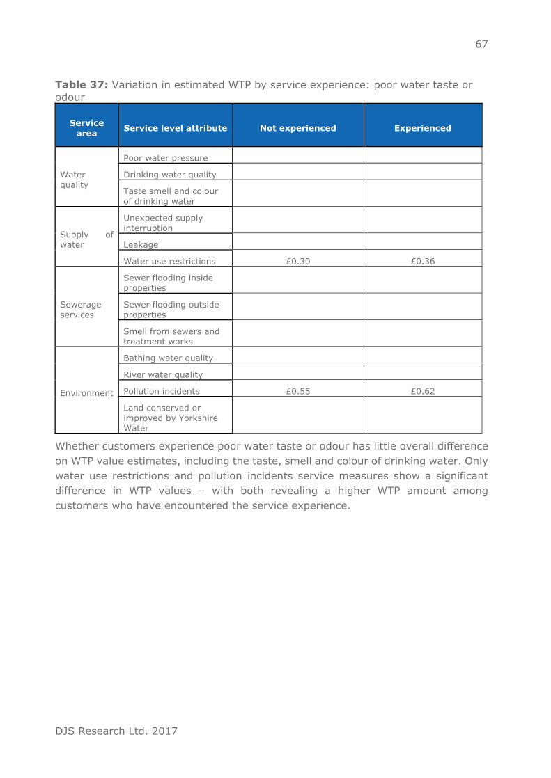
67


Table 37: Variation in estimated WTP by service experience: poor water taste or

odour

Service area

Service level attribute Not experienced Experienced

Water quality

Poor water pressure



Supply of water


Leakage


Sewerage services




Environment


River water quality


Land conserved or


Whether customers experience poor water taste or odour has little overall difference

on WTP value estimates, including the taste, smell and colour of drinking water. Only

water use restrictions and pollution incidents service measures show a significant

difference in WTP values – with both revealing a higher WTP amount among

customers who have encountered the service experience.

68


Table 38: Variation in estimated WTP by service experience: sewer flooding inside your property

Service

area Service level attribute Not experienced Experienced

Water quality



Taste smell and colour

of drinking water £2.14 £3.02

Supply of water


Leakage £0.76 £0.96


Sewerage services

Sewer flooding inside properties £0.90 £1.44


Smell from sewers and treatment works £0.58 £0.68

Environment




Land conserved or improved by Yorkshire Water £0.55 £0.90

When comparing customers who have experienced sewer flooding inside their

property with those who haven’t, significant differences across 11 of the 13 service

measures occur. In each of the 11 service areas with significant differences, those

who have experienced sewer flooding inside their property have a higher WTP value

than those who haven’t had the experience – suggesting that having a service

experience with potentially severe outcomes can result in higher levels of WTP for

services across a variety of measures.

69


Table 39: Variation in estimated WTP by service experience: Sewer flooding in your garden or close to your property

Service


Water quality





Supply of water

Unexpected supply interruption £0.80 £1.04

Leakage


Sewerage services




Environment





Although not as marked as the comparative outcomes for sewer flooding inside a

property, customers who have experienced sewer flooding outside also show a higher

WTP propensity – this time across 8 of the 13 service measures. Interestingly, the

WTP value for sewer flooding outside of properties across the two groups is not

significantly different, suggesting that in some scenarios the experience has an

impact on the individual’s wider attitude (or WTP) towards water service, but not on

the actual measure by which they were affected.

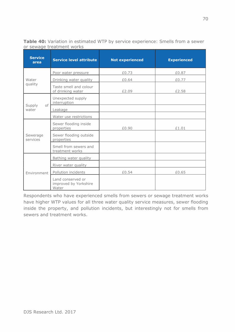
70


Table 40: Variation in estimated WTP by service experience: Smells from a sewer or sewage treatment works

Service


Water quality





Supply of water


Leakage


Sewerage services




Environment


River water quality



Respondents who have experienced smells from sewers or sewage treatment works

have higher WTP values for all three water quality service measures, sewer flooding

inside the property, and pollution incidents, but interestingly not for smells from

sewers and treatment works.

71


Table 41: Variation in estimated WTP by service experience: A leaking water

supply pipe on your property

Service area


Water

quality




Supply of water

Unexpected supply

interruption

Leakage


Sewerage services




treatment works

Environment


River water quality


Land conserved or

improved by Yorkshire Water £0.55 £0.71

Customers who have experienced a leaking supply pipe in the past have a higher

estimated WTP across all three water quality service measures than those who

haven’t experienced a leaking supply pipe in the past. As with some other

experiences, despite the issue in question having a significant impact on the WTP

estimates of a number of service measures, it doesn’t appear to have any impact on

the WTP value of the experience in question (Leakage); this could be because the

leak was on their own pipes and not those external to their properties.

72


Table 42: Variation in estimated WTP by service experience: A leaking water

supply pipe close to your property

Service area


Water

quality




Supply of water


Leakage £0.72 £0.97


Sewerage services




Environment





Experience of a leaking supply pipe close to the property has an interesting impact

on WTP estimates across the four environment service measures. In each case those

with prior experience of the external leaking supply pipe close to their property have

a higher WTP estimate than those who haven’t had the experience.

73


Table 43: Variation in estimated WTP by service experience: Low water pressure

Service


Water quality

Poor water pressure



Supply of water


Leakage


Sewerage

services



properties


treatment works

Environment


River water quality

Pollution incidents


Despite low water pressure being a service measure with a high proportion of

significant differences by sub-group analysis, when those who have and haven’t

experienced it in the past are compared, only one significant difference emerges –

the taste, smell and colour of drinking water, which is the service measure with the

highest level of WTP estimate overall. This suggests that although perceptions (and

there for WTP) are different across a number of groups, the actual impact of

experiencing it doesn’t unduly affect wider attitudes towards water supply and

service.

74


Table 44: Variation in estimated WTP by service experience: Restriction on how you can use water (e.g. a hosepipe ban)

Service area


Water quality




Supply of

water


Leakage


Sewerage

services



properties


Environment


River water quality

Pollution incidents


Experience of water use restrictions in the past has a significant impact on the WTP

estimates for this service measure as well as three water quality service measures,

sewer flooding inside properties, smells from sewers and sewage treatment works.

In each case the WTP estimate is higher for those that have had the experience than

those who haven’t.

75


Table 45: Variation in estimated WTP by service experience: An instruction to boil

your drinking water

Service area


Water quality




£2.10 £2.59

Supply of water


Leakage £0.75 £0.91


Sewerage services


£0.89 £1.08


£0.55 £0.64


Environment




Land conserved or


When customers who have experienced drinking water boil notices are compared

against those who haven’t had the experience, significant differences in WTP

estimates occur across 9 of the 13 service measures – including across all three water

quality service measures.

76


Use and non-use valuations

The WTP and WTA estimates provided in this report have been total economic

valuations, meaning they contain both the ‘use’ values (the value the respondent

places on the services they receive and use) and the ‘non-use’ values (the indirect

value that the respondent places on the water service for altruistic reasons). To

measure the amount of use and non-use value each respondent places on Water

Services, the survey questionnaire included a raft of attitudinal questions.

Respondents attitudes to protecting Yorkshire Water’s land and water environments

such as lakes, rivers, bathing waters, woodlands, and grasslands were evaluated via

a series of questions including ‘it is important to me because I like to visit for

recreational purpose’ (a ‘use’ value) and ‘it is important to me because I want future

generations to be able to enjoy them’ (a non-use value). A composite score based

on the combined responses to the ‘use’ statements was created as was a composite

score of ‘non-use’ statements.

To test the extent to which these use and non-use composite scores impact on WTP

estimate for each service level, the use and non-use variables were included as choice

invariant variables within the Conditional Logit model.

Table 46: Conditional Logit model use and non-use choice invariant variables coefficients

Non-use Use

Water quality

0.118 (p=0.023) 0.394 (p=0.000)

Supply of

Water 0.061(p=0.039) 0.551(p=0.020)

Sewerage services

0.070(p=0.036) 0.530(p=0.021)

Environment 0.170(p=0.000) 0.375(p=0.000)

77


Table 47: Conditional Logit model margin WTP divided into Use and non-use

Values

Per +1 level

increase based on Conditional

Logit model

Marginal WTP Use Non–use

Poor water pressure £0.75 £0.57 £0.17

Drinking water quality £0.66 £0.50 £0.15

Taste, smell and colour of drinking

water

£2.17 £1.67 £0.50


£0.81 £0.73 £0.08

Leakage £0.77 £0.70 £0.08

Water use restrictions £0.31 £0.27 £0.03


£0.92 £0.81 £0.11


£0.56 £0.50 £0.07

Properties subjected to chronic (seasonal) unbearable smells from sewers & treatment works: complaints to

Yorkshire Water per year

£0.58 £0.51 £0.07



£0.40 £0.28 £0.13

Length of rivers in Yorkshire improved

(%)

£1.11 £0.76 £0.35

Category 3 pollution incident: a minor incident that has a

minimal impact on the quality of water in the area

£0.56 £0.38 £0.17

Area of land conserved

or improved by Yorkshire Water

£0.56 £0.38 £0.17

78


‘Non-use’ WTP estimates are higher for the environment service areas than they are

for the other water and sewerage services. Conversely, ‘use’ estimates are higher for

the water and sewerage services.

Validity of survey results

We conclude our analysis of the household survey with evidence on our validity

checking.

After the choice experiment blocks, respondents were asked to select from a pre-

coded list, which two statements (a first choice and a second choice) came closest to

describing the rationale behind their choices. The chart below shows the overall

decision-making choices of the household sample.

Figure 9: decision-making rationale

I chose the options…

Base: all household respondents

79


Making choices based on realistic and easy to understand levels of service

To understand the extent to which respondents understood the choice experiments,

and the extent to which they felt the levels of service (and associated costs) realistic,

two questions were asked. Firstly, ‘did you feel able to make comparisons between

the choices I presented to you?’ and secondly, ‘In the choices did you find each of

the levels of service we described, realistic and easy to understand?’.

Figure 10: ability to make comparisons, and the ease of understanding service levels

For both questions, just over 9 in 10 said they were able to make comparisons, and

that the service levels were realistic and easy to understand.

The one in ten who said ‘no’ to each question were asked for the reason why. Answers

were similar for both and centred around customers finding the information too much

or too complicated:

“It was complicated to differentiate between all the choices and you just tend

to not want prices to rise”

“It was quite difficult to compare all the choices and decide the best option”

“There were so many comparisons and so much information it started to cloud

my mind”

80


“I couldn’t care less about the options and there was far too much information

about things, I don’t care about, homes affected by something or other”

Ease of understanding is significantly higher than the levels of understanding

reported in the PR14 exercise where 73.7% of respondents found the choice

experiment tasks understandable.

Construct validity

In order to assess the construct validity, we interrogate the results in terms of how

well they conform with our a priori expectations and uphold statistical theory.

The direction of signs of all of the coefficients observed in this study are consistent

with our expectations. For example, Utility increases as water service levels increase

and Utility decreases as bill impacts increase.

In terms of statistical validity, the models provide a good fit to the data. A pseudo-

𝑅2 value of 0.12 is considered good for Conditional Logit models employing cross-

sectional data (Breffle and Rowe, 2002), and many studies have reported lower

pseudo-𝑅2 values. All the models presented display good model fit.

In addition, the results also conform to economic theory in terms of variables

explaining choices.

81


Appendix 2 – results and

findings, business Introduction

This section of the report presents the main findings from the Work Package 1

business survey. Target quotas were applied to region, sector and the number of

employees to ensure a diverse sample of businesses were consulted.

A total of 542 interviews were conducted with business customers, with a split of 246

online interviews and 296 CAPI interviews.

Business respondent profile

The images below show a demographic sample overview of the businesses consulted

during fieldwork.

Figure 11: Business sample

Sub-group analysis

The analysis section of this report includes data and analysis of various business

customer groups. Firstly, sample groups as outlined above are analysed, and any

differences in attitude or outcome are either presented in chart form, or discussed in

the report commentary. In addition, a further set of business customers are

analysed:

• Water critical nature of the business

82


All respondents were asked how critical the Supply of Water is to their business being

able to operate. The chart below shows the breakdown of responses to this question:

Figure 12: criticalness of water supply to the business

Base: all business customers, excluding don’t know responses (as shown)

Service experiences

In order to include an additional layer of understanding to reactions in the stated

preference exercises, respondents were asked whether their business had ever

experienced any of the following service experiences in Yorkshire. The table below

shows the proportion of respondents reporting having experienced each issue.

Figure 13: Service experiences

Base: all business respondents excluding don’t know per issue (as shown)

83


Analysis and results

This section of the report contains analysis of the business Willingness to Pay (WTP),

with a broad structure of the findings outlined as follows:

• Examination of the preference for the status quo

• Results from each model

• The final/preferred WTP table for each of the 4 CE blocks

• Results of the full-package CE

• The validity of the outcomes

The tables below summarise the choice behaviour observed with the business customer sample.

Table 48: Choice frequencies for business samples

Status quo Alternative 1 Alternative 2





Table 49: Proportion of serial status quo choices and bill reduction option choices

Always choose

status quo

Always choose

bill increases

Always choose

bill reductions





Table 48 shows that the status quo is selected at least half of the time for Water

Quality and Sewerage services, and just under half of the time for Supply of Water

and Environment - revealing a very high level of choice of the status quo option with

two service area blocks. Environmental services have the largest deviation from the

status quo.

Table 49, meanwhile, shows the percentage of respondents who always select the

status quo (or increases or decreases) – showing that around a third of business

84


respondents consistently choose the status quo when given multiple choices. The

remainder of respondents select different options across the CE sets within the

blocks.

Block 1 - Water Quality

After extensive analysis of the data, three models were considered to describe the

choice data obtained from the business customers. The first was a simple Conditional

Logit model, while the other two were the Random Parameter Logit model and the

Generalised Mixed Logit.

For the water quality choice set based on CE1, the Generalised Mixed Logit model

performed best in terms of goodness-of-fit to the data with a Pseudo 𝑅2 = 0.16

(compared with 0.16 for the Random Parameter Logit model, and 0.14 for the


assumed to be normally distributed with respect to the service measures s (poor

water pressure, drinking water quality and taste, smell and colour of drinking water);

but the bill coefficient was assumed to be fixed, as was the status quo coefficient.


of the water quality in the models conformed to prior expectations, i.e. as the service


highly statistically significant at the 1% level. The coefficient for the status quo choice




85


Table 50: Models of Water Quality choice data



Logit



Poor water pressure: number of properties

below standard

pressure

0.15184 0.0000 0.1186 0.0000 0.178656 0.0000

Drinking

water quality: the proportion of samples of tap water that will pass the

DWI’s (a government body) requirement for chemical & biological

content

0.17285 0.0000 0.2283 0.0000 0.19979 0.0000

Taste, smell & colour of drinking

water: total number of water quality contacts

0.55123 0.0000 0.532213 0.0000 0.511231 0.0000

Bill impact -0.496582 0.0000 -0.31135 0.0000 -0.51123 0.0000

Status quo 0.50755 0.0000 0.58539 0.0000 0.586236 0.0000


in Table 51. Based on the Conditional Logit model, business customers were prepared

to pay on average 0.2% more on their bill for each increase in drinking water quality

service level. Table 51 also reports the 95% confidence intervals associated with

marginal WTP for all three models.

86


The RPL model, which is linear, suggests that the average business customer is willing

to pay an additional 0.72% for a single level increase in taste, smell and colour of

drinking water.

Table 51: WTP results for water quality choice data



Logit

Marginal

WTP

95%

LL 95%UL

Marginal

WTP

95%

LL 95%UL

Marginal

WTP

95%

LL 95%UL

Poor water pressure

0.18% 0.10% 0.25% 0.14% 0.10% 0.17% 0.20% 0.13% 0.28%


0.20% 0.13% 0.27% 0.26% 0.19% 0.34% 0.23% 0.16% 0.30%

Taste, smell and colour of drinking water

0.64% 0.56% 0.72% 0.61% 0.55% 0.67% 0.58% 0.53% 0.63%


between WTP and the level of service they receive. However as previously suggested,

utility increases at a decreasing rate as the service measure level improves. Such a

non-linear utility function can be modelled with a non-linear function; but an

alternative is to model the non-linear relationship through a piecewise regression

model (i.e. a fixed effects model). A non-linear utility change model or fixed effects

model is therefore used to assess whether a non-linear relationship holds for service

improvements and service reductions.

The non-linear utility change model, or fixed effects model, was estimated using each

of the three models used above. While the Generalised Mixed Logit and Random

Parameter Logit models provide a better fit with the data they do not provide

statistically significant coefficient values for a number of the service measure effects.

Given that the purpose of this exercise is to estimate customer WTP for improvements

in service measure levels it was decided to base the following discussion on the

Conditional Logit model (see Table 52), where most coefficient values are significant

and capable of meaningful interpretation.

In this model most coefficients change monotonically: for example, drinking water

quality(L-2) < drinking water quality(L-1) < drinking water quality(L+1) < drinking

water quality(L+2).

87


Table 52: Non-Linear Conditional Logit model for Water Quality


Observations = 9180



-0.51304 0.000 -0.52% -0.71% -0.33%


-0.19924 0.115 -0.20% -0.45% 0.05%

Poor water

pressure (L+1) 0.198653 0.000 0.20% 0.12% 0.28%

Poor water

pressure (L+2) 0.265986 0.000 0.27% 0.21% 0.32%


0.28465 0.000 0.29% 0.23% 0.35%


-0.68317 0.000 -0.69% -0.96% -0.42%

Drinking water

quality (L-1) -0.37391 0.006 -0.38% -0.61% -0.15%


0.25903 0.051 0.26% 0.16% 0.37%


0.3665 0.000 0.37% 0.28% 0.46%


0.3907 0.001 0.40% 0.29% 0.51%


-0.90374 0.001 -0.92% -1.07% -0.76%


-0.42005 0.000 -0.43% -0.52% -0.33%


0.56083 0.0009 0.57% 0.47% 0.67%


1.19731 0.0000 1.21% 0.96% 1.47%

Taste, smell and

colour of drinking

water (L+3)

1.3929 0.0000 1.41% 1.23% 1.59%

Bill impact -0.32155 0.0000

The results of the fixed effects model indicate that the average business customer

would be prepared to pay a +0.37% increase on their water bill to increase drinking

water quality level from the status quo to level +2. The average customer would be

willing to accept a decrease in taste, smell and colour of drinking water to level -1

for a bill reduction of -0.43% per year.

88


Overall, the fixed effect model for Water Quality indicates that there is diminishing





Block 2 – Supply of Water

Again, the 3 models were applied to the data relating to CE2, Supply of Water.

For the Supply of Water choice set based on CE2, the Random Parameter Logit model




assumed to be normally distributed with respect to the service measures s

(unexpected supply interruption, leakage and water use restrictions); but the bill

coefficient was assumed to be fixed, as was the status quo coefficient.


of the Supply of Water in the models conformed to prior expectations, i.e. as the






Table 53: Models of Supply of Water choice data


Logit

Generalised Mixed

Logit



Unexpected supply interruption of 3–6 hours: total properties

affected

0.42834 0.0000 0.39569 0.0000 0.456554 0.0000

Leakage 0.40739 0.0000 0.454667 0.0000 0.485652 0.0000


0.14506 0.0000 0.17344 0.0338 0.123357 0.0000

Bill impact -0.26257 0.0000 -0.25292 0.02825 -0.26684 0.0000

Status quo 0.28764 0.0155 0.25963 0.0006 0.33237 0.00012

89




to pay on average +0.24% more on their bill for each increase in the unexpected

service interruption level. Table 54 also reports the 95% confidence intervals

associated with marginal WTP for all three models.

Table 54: WTP results for Supply of Water choice data


Logit

Generalised Mixed

Logit

Marginal

WTP

95%

LL 95%UL

Marginal

WTP

95%

LL 95%UL

Marginal

WTP

95%

LL 95%UL

Unexpected

supply interruption of 3–6 hours: total properties affected

0.24% 0.21% 0.28% 0.21% 0.18% 0.24% 0.22% 0.20% 0.24%

Leakage 0.20% 0.17% 0.24% 0.25% 0.19% 0.30% 0.21% 0.18% 0.25%


0.08% 0.04% 0.11% 0.06% 0.04% 0.09% 0.09% 0.05% 0.12%


between WTP and the level of service they receive. However the alternative is to




service reductions.




90


Table 55: Non-Linear Conditional Logit model for Supply of Water


Observations = 9180


Unexpected

supply interruption of 3–6 hours: total properties affected (L-2)

-0.71762 0.000 -0.37% -0.49% -0.25%

Unexpected supply

interruption of 3–6 hours: total properties

affected (L-1)

-0.45257 0.000 -0.23% -0.35% -0.11%

Unexpected supply interruption of 3–

6 hours: total properties affected (L+1)

0.21534 0.040 0.11% 0.05% 0.17%

Unexpected

supply interruption of 3–6 hours: total properties affected (L+2)

0.49483 0.000 0.26% 0.17% 0.34%

Unexpected supply interruption of 3–6 hours: total properties affected (L+3)

0.5411 0.000 0.28% 0.18% 0.38%

Leakage (L-2) -0.81375 0.000 -0.42% -0.56% -0.28%

Leakage (L-1) -0.71435 0.000 -0.37% -0.49% -0.25%

Leakage (L+1) 0.25838 0.017 0.13% 0.06% 0.20%

Leakage (L+2) 0.4681 0.018 0.24% 0.19% 0.30%

Leakage (L+3) 0.4953 0.021 0.26% 0.20% 0.32%

Water use restrictions e.g. hose pipe ban (L-2)

-0.34481 0.002 -0.18% -0.29% -0.07%

Water use restrictions e.g. hose pipe ban (L-1)

-0.10585 0.018 -0.05% -0.10% -0.01%

91


Water use restrictions e.g. hose pipe ban (L+1)

0.16195 0.022 0.08% 0.05% 0.12%


0.2873 0.015 0.15% 0.09% 0.21%


0.4012 0.013 0.21% 0.14% 0.28%

Bill impact -0.36591 0.000


would be prepared to pay a +0.24% increase on their water bill to increase leakage

level from the status quo to level +2. The average customer would be willing to

accept a decrease in leakage to level -1 for a bill reduction of -0.37% per year.

Overall, the fixed effect model for Supply of Water indicates that there is diminishing





Block 3 – Sewerage Services

Again, the 3 models were applied to the data relating to CE3, sewerage services.

For the sewerage services choice set based on CE3, the Conditional Logit model


(compared with 0.21 for the Generalised Mixed Logit model, and 0.21 for the Random

Parameter Logit model). In the Random Parameter Logit model, tastes were assumed

to be normally distributed with respect to the service measures (sewer flooding inside

properties; number of incidents per year, sewer flooding outside properties; number

of incidents per year and properties subjected to chronic (seasonal) unbearable

smells from sewers & treatment works: complaints to Yorkshire Water per year); but

the bill coefficient was assumed to be fixed, as was the status quo coefficient.


of the sewerage services in the models conformed to prior expectations, i.e. as the





92


Table 56: Models of Sewerage Services choice data


Logit

Generalised Mixed

Logit



Sewer flooding

inside properties: number of incidents per year

0.44571 0.0000 0.39687 0.0000 0.468798 0.0000

Sewer flooding outside properties: number of

incidents per year

0.19914 0.0000 0.14827 0.0000 0.213569 0.0000

Properties subjected

to chronic (seasonal)

unbearable smells from sewers & treatment

works: complaints to Yorkshire Water per year

0.21424 0.0000 0.20819 0.0000 0.221312 0.0000

Bill impact -0.85406 0.0000 -0.72337 0.0000 -0.80002 0.0000

Status quo 0.23 0.0000 0.22044 0.0000 0.24569 0.0000



to pay on average +0.29% more on their bill for each increase in sewer flooding

inside properties; number of incidents per year service level. Table 57 also reports

the 95% confidence intervals associated with marginal WTP for all three models.

The Random Parameter Logit model suggests that the average business customer is

willing to pay an additional +£0.52 for a level increase in properties subjected to

93


chronic (seasonal) unbearable smells from sewers & treatment works: complaints to

Yorkshire Water per year.

Table 57: WTP results for sewerage services choice data



Logit

Marginal

WTP

95%

LL 95%UL

Marginal

WTP

95%

LL 95%UL

Marginal

WTP

95%

LL 95%UL

Sewer flooding

inside properties;

number of incidents per year

0.29% 0.27% 0.31% 0.30% 0.26% 0.33% 0.29% 0.25% 0.33%

Sewer

flooding outside properties; number of incidents per year

0.13% 0.10% 0.16% 0.11% 0.07% 0.15% 0.13% 0.11% 0.16%


unbearable smells from sewers & treatment works: complaints


0.14% 0.11% 0.17% 0.15% 0.12% 0.19% 0.14% 0.11% 0.16%






service reductions.




94


Table 58: Non-Linear Conditional Logit model for sewerage services


Observations

= 9180 Coefficient Prob.|z|>Z Marginal WTP 95% LL 95%UL

Sewer flooding

inside properties; number of


-0.79644 0.000 -0.45% -0.58% -0.32%

Sewer flooding

inside properties; number of incidents per year (L-1)

-0.50168 0.000 -0.28% -0.41% -0.15%

Sewer flooding inside properties; number of incidents per year (L+1)

0.21766 0.000 0.12% 0.07% 0.17%

Sewer flooding

inside properties; number of incidents per year (L+2)

0.46589 0.000 0.26% 0.18% 0.34%

Sewer flooding inside properties; number of incidents per year (L+3)

0.6012 0.000 0.34% 0.25% 0.43%

Sewer flooding outside properties; number of


-0.35074 0.005 -0.20% -0.33% -0.06%


properties; number of incidents per year (L-1)

-0.21781 0.059 -0.12% -0.25% 0.00%

Sewer flooding outside properties; number of incidents per year (L+1)

0.205264 0.000 0.12% 0.10% 0.13%

95


Sewer flooding outside properties; number of incidents per

year (L+2)

0.35074 0.000 0.20% 0.17% 0.23%

Sewer flooding outside properties;

number of incidents per year (L+3)

0.3798 0.000 0.21% 0.17% 0.25%

Properties

subjected to chronic

(seasonal) unbearable smells from sewers & treatment works:

complaints to Yorkshire Water per year (L-2)

-0.39677 0.003 -0.22% -0.34% -0.11%

Properties

subjected to chronic (seasonal) unbearable smells from sewers &

treatment works:

complaints to Yorkshire Water per year (L-1)

-0.15008 0.027 -0.08% -0.08% -0.09%

Properties subjected to chronic (seasonal) unbearable smells from sewers &

treatment works: complaints to Yorkshire Water per year (L+1)

0.20546 0.036 0.12% 0.07% 0.16%

Properties subjected to

chronic (seasonal) unbearable smells from

sewers & treatment works: complaints to Yorkshire Water per year (L+2)

0.44463 0.000 0.25% 0.12% 0.38%


0.5146 0.000 0.29% 0.20% 0.38%

96


unbearable smells from sewers & treatment works: complaints to

Yorkshire Water per year (L+3)

Bill impact -0.41017 0.000


would be prepared to pay a +0.26% increase on their water bill to increase sewer

flooding inside properties; number of incidents per year level from the status quo to

level +2. The average customer would be willing to accept a decrease in properties

subjected to chronic (seasonal) unbearable smells from sewers & treatment works to

level -1 for a bill reduction of -0.08% per year.

Overall, the fixed effect model for sewerage services indicates that there is

diminishing marginal utility for improvements in some service measure levels; and

also, asymmetry between WTP for improvements in service levels and WTA

(compensation or bill reductions) for a lower level of service. This suggests the non-

linear approach is superior to the linear assumptions of the previous models.

Block 4 – Environment

For the environment choice set based on CE4, the Conditional Logit model performed

best in terms of goodness-of-fit to the data with a Pseudo 𝑅2 = 0.21 (compared with

0.19 for the Generalised Mixed Logit model, and 0.20 for the Random Parameter

Logit model). In the Random Parameter Logit model, tastes were assumed to be

normally distributed with respect to the service measures s (number of bathing

beaches meeting ‘Good’ or ‘Excellent’ standard, length of rivers in Yorkshire improved

(%), category 3 pollution incident: a minor incident that has a minimal impact on the

quality of water in the area, and area of land conserved or improved by Yorkshire

Water); but the bill coefficient was assumed to be fixed, as was the status quo

coefficient.


of the environment in the models conformed to prior expectations, i.e. as the service


statistically significant at the 5% level. The coefficient for the status quo choice is

positive and statistically significant suggesting that the presence of the status quo


97


Table 59: Models of Environment choice data



Logit




‘Good’ or ‘Excellent’

standard

0.16619 0.0000 0.131222 0.0000 0.189756 0.0000

Length of


0.45885 0.0000 0.44395 0.0013 0.42316 0.0000

Category 3 pollution incident: a minor incident

that has a minimal impact on the

quality of water in the area

0.22186 0.0000 0.21825 0.0000 0.213569 0.0000



0.12092 0.0000 0.20951 0.0365 0.132695 0.0000

Bill impact

-0.17756 0.0000 -0.30226 0.0018 -0.18988 0.0000

Status quo

0.1787 0.0029 0.1702 0.00512 0.199898 0.0000


in Table 60 Based on the Conditional Logit model, business customers were prepared

to pay on average +0.39% more on their bill for each increase in length of rivers in

Yorkshire improved (%) service level. Table 60 also reports the 95% confidence

intervals associated with marginal WTP for all three models.

98


Table 60: WTP results for environment choice data



Logit

Marginal

WTP

95%

LL 95%UL

Marginal

WTP

95%

LL 95%UL

Marginal

WTP

95%

LL 95%UL



0.14% 0.09% 0.19% 0.15% 0.10% 0.20% 0.16% 0.10% 0.22%

Length of


0.39% 0.33% 0.44% 0.35% 0.29% 0.41% 0.36% 0.32% 0.40%

Category 3 pollution incident: a minor incident that has a minimal

impact on the quality of water in the area

0.19% 0.14% 0.24% 0.21% 0.14% 0.27% 0.18% 0.14% 0.22%


Yorkshire Water

0.10% 0.06% 0.15% 0.11% 0.07% 0.14% 0.11% 0.06% 0.16%






service reductions.




99


Table 61: Non-Linear Conditional Logit model for environment


Observations = 9180


Number of

bathing beaches meeting ‘Good’ or ‘Excellent’ standard (L-2) -0.4475 0.000 -0.36% -0.54% -0.19%


or ‘Excellent’ standard (L-1) -0.2112 0.000 -0.17% -0.32% -0.03%

Number of bathing beaches meeting ‘Good’ or ‘Excellent’ standard (L+1) 0.1632 0.022 0.13% 0.08% 0.19%


standard (L+2) 0.19526 0.000 0.16% 0.10% 0.22%


or ‘Excellent’ standard (L+3) 0.2612 0.000 0.21% 0.14% 0.28%


improved (%) (L-2) -0.88092 0.000 -0.72% -0.60% -0.83%


improved (%) (L-1) -0.42666 0.001 -0.35% -0.54% -0.15%


improved (%) (L+1) 0.49391 0.017 0.40% 0.27% 0.53%

Length of rivers

in Yorkshire

improved (%) (L+2) 0.89268 0.011 0.73% 0.57% 0.88%

Length of rivers

in Yorkshire improved (%) (L+3) 0.9031 0.000 0.74% 0.58% 0.90%

Category 3

pollution incident: a minor incident that has a minimal impact -0.50342 0.000 -0.41% -0.63% -0.19%

100


on the quality of water in the area (L-2)

Category 3 pollution incident: a minor incident that has a minimal impact on the quality of

water in the area (L-1) -0.2775 0.032 -0.23% -0.26% -0.19%

Category 3 pollution

incident: a minor incident that has

a minimal impact on the quality of water in the area (L+1) 0.2042 0.008 0.17% 0.11% 0.22%

Category 3 pollution incident: a minor incident that has a minimal impact

on the quality of water in the area (L+2) 0.4053 0.002 0.33% 0.22% 0.44%

Category 3 pollution incident: a minor incident that has

a minimal impact on the quality of water in the area

(L+3) 0.5542 0.000 0.45% 0.36% 0.54%


Yorkshire Water (L-2) -0.35701 0.003 -0.29% -0.48% -0.10%


improved by Yorkshire Water (L-1) -0.28461 0.002 -0.23% -0.29% -0.17%

Area of land

conserved or improved by Yorkshire Water (L+1) 0.0836 0.050 0.07% 0.00% 0.13%

Area of land conserved or improved by Yorkshire Water (L+2) 0.12791 0.030 0.10% 0.05% 0.15%

Area of land conserved or improved by 0.1295 0.045 0.11% 0.05% 0.17%

101


Yorkshire Water (L+3)

Bill impact -0.27049 0.000 -


would be prepared to pay a +0.73% increase on their water bill to increase length of

rivers in Yorkshire improved (%) level from the status quo to level +2. The average

customer would be willing to accept a decrease in area of land conserved or improved

by Yorkshire Water to level -1 for a bill reduction of 0.23% per year.

Overall, the fixed effect model for environment indicates that there is diminishing





102


Willingness to Pay estimates

The final WTP and WTA based on the non-linear model estimates for business

customers are summarised in table 62. In almost all of the service level areas

considered, the level of WTA is greater than the level of WTP for the greatest service

decrease or increase.

Table 62: WTP and WTA estimates – all levels Business Customers

Service

area

Service level

attribute

Willingness to Pay

Reduction in service


-1 +1 +2 +3

Water quality

Poor water pressure: number of properties below standard pressure

-0.20% 0.20% 0.27% 0.29%

Drinking water quality: the proportion of samples of tap water that will pass the DWI’s (a government body) requirement for

chemical & biological content

-0.38% 0.26% 0.37% 0.40%

Taste, smell & colour of drinking water: total

number of water quality contacts

-0.43% 0.57% 1.21% 1.41%

Supply of Water

Unexpected supply interruption of 3–6 hours:

total properties affected

-0.23% 0.11% 0.26% 0.28%

Leakage -0.37% 0.13% 0.24% 0.26%

Water use restrictions e.g.

hose pipe ban -0.05% 0.08% 0.15% 0.21%

Sewerage services


-0.28% 0.12% 0.26% 0.34%


-0.12% 0.12% 0.20% 0.21%

Properties subjected to

chronic (seasonal) unbearable smells from sewers & treatment works: complaints to Yorkshire Water per year

-0.08% 0.12% 0.25% 0.29%

Environment

Number of bathing beaches meeting ‘Good’ or ‘Excellent’ standard

-0.17% 0.13% 0.16% 0.21%


-0.35% 0.40% 0.73% 0.74%

103



-0.23% 0.17% 0.33% 0.45%


-0.23% 0.07% 0.10% 0.11%

Full package CE

In the final choice experiment, CE5, respondents were presented with the full

package of 13 service levels shown at highest levels of service (L+2) at a range of

bill impacts for the total package (7%, 12%, 16%, 20%, 25%, 30%).

The level of acceptance declines at each increased water bill impact. In each case,

the status quo is preferred to the alternative scenario.

Table 63: CE5 choice by scenario at each bill impact - Business

Alternative scenario (L+2) Status quo – no bill impact

7% 43.8% 56.3%

12% 33.0% 67.0%

16% 34.7% 65.3%

20% 27.6% 72.4%

25% 24.1% 75.9%

30% 24.2% 75.8%

Content validity

Following the series of choice experiments, respondents were asked to offer reasons

for the way they had made their selections. The most frequently mentioned reasons

for choice was ‘least cost to business’ which was mentioned by 53% of respondents.

This was closely followed by ‘offers the most improvements relative to cost’ with 46%

of respondents reporting this was a reason behind their choice.

15% of business respondents mentioned their choices were altruistic and would

benefit other customers. Only 24 respondents (4% of the sample) mentioned that

they felt the information presented to them was not clear enough to make their

choice.

104


Table 64: Motivations for choice in the CEs

Reasons for choice %

I chose the options that would cost the least to the business 53%

I chose the options which I thought offered the most improvements relative to cost

46%

I chose improvements that I thought would be most likely to benefit the environment

25%

I chose the options that affect or are most likely to affect my business directly

25%

I chose the options that I thought would benefit people and businesses I know

21%

I chose the options that I thought would benefit others the most 15%

The information provided was not clear enough for me to make a choice 4%

In addition, two further questions relating to how well they felt they could make

choices in the experiment and how realistic they found the scenarios presented to

them. The levels of ease of understanding amongst business customers is higher

than the levels reported in PR14 where 70.8% of business customers reported that

the choice experiment task was easy to understand.

Did you feel able to make comparisons between the choices I presented to you?

Reasons for choice %

Yes 91%

No 9%

In the choices, did you find each of the levels of service we described, realistic and

easy to understand?

Levels were realistic and easy to understand

%

Yes 90%

No 10%

105


The one in ten who said ‘no’ to each question were asked for the reason why. Answers

were similar for both and centred around business customers finding the information

too complicated or too little variation between the options:

“I didn’t feel there were much between the options to justify the increases”

“Of necessity in a survey like this, the level of detail is quite low

“It wasn’t very clear what the differences actually were.”

“Quite a few ... I had to really concentrate”

Construct validity

In order to assess the construct validity, we interrogate the results in terms of how

well they conform with our a priori expectations and uphold statistical theory.

The direction of signs of all of the coefficients observed in this study are consistent

with our expectations. For example, Utility increases as water service levels increase

and Utility decreases as bill impacts increase.

In terms of statistical validity, the models provide a good fit to the data. A pseudo-

𝑅2 value of 0.12 is considered good for Conditional Logit models employing cross-

sectional data (Breffle and Rowe, 2002), and many studies have reported lower

pseudo-𝑅2 values. All the models presented display good model fit.

106


Appendix 5e: Understanding Customer Values …...This work package used stated preference methods to...

Documents

Transcript of Appendix 5e: Understanding Customer Values …...This work package used stated preference methods to...