State and Local SpendingDo Tax and Expenditure Limits Work?

Benjamin Zycher

May 2013

A M E R I C A N E N T E R P R I S E I N S T I T U T E

Executive Summary

Since 1978, 30 states have enacted formal limitations on taxes, budgets, or outlays as

tools with which to strengthen fiscal discipline. These tax and expenditure limits (TELs)

vary substantially in terms of their details, definitions, and underlying structures, but the

empirical finding reported here is simple and powerful: TELs are not effective.

It is no secret that the fiscal pressures facing states and localities are likely to

intensify sharply in the near future. These pressures are reflected in the rising share of

federal finance (or revenue transfers) observed in state and local spending over time,

driven heavily by health care programs, Medicaid in particular. Future pension liabilities

also are a prominent source of the growing fiscal crisis that states and localities are

beginning to confront. These pressures will inevitably strengthen demands that the

federal government increase its transfers to lower levels of government.

The empirical analysis reported here applies data from 49 states (excluding

Alaska) over the period 1970–2010 to the empirical question of the effectiveness of

TELs, which across the states display a wide variety of features. The ineffectiveness of

TELs is unambiguous in terms of summary statistics, case-study examination of the

records of several individual states, and estimation of an econometric model. This model

was estimated for both state and local spending combined and state outlays considered

alone. The econometric model estimated here differs from those in the earlier literature,

most importantly in that the existence of a TEL in a given state is treated here as a

decision variable. The finding of ineffectiveness is broadly consistent with the findings

reported in the earlier peer-reviewed literature.

The almost-universal weakness of TELs is striking, but the empirical evidence by

itself does not explain these findings. In part, it is likely that the limits themselves are the

products of the same political pressures and election dynamics that yield fiscal outcomes.

Moreover, the competition among political interests that results in budget outcomes also

is likely to weaken or circumvent limits that otherwise would be effective. This raises a

larger overall question: what are the sources of government growth? Five hypotheses are

discussed in this study, the upshot of which is that TELs by themselves are unlikely to

affect the demand for or the cost of government spending.

2

The findings reported here should interest state (and local) officials seeking ways

to reduce or to neutralize powerful pressures for spending and revenue growth. They

should also interest federal policymakers subjected to state and local demands for

revenue transfers and others kinds of aid; a quid pro quo in the form of a tax or

expenditure limitation is very unlikely to reduce future pressures for additional federal

aid. Moreover, they should interest the broader policy community as state and local (and

federal) fiscal problems intensify, and with them the public discussion of alternative

policy responses, and the public, ultimately the source of all resources consumed or

allocated by government.

It is likely to be the case that such mechanical tools as TELs cannot substitute for

the hard work of long-term public education and persuasion about the central benefits of

limited government. In the long run under democratic institutions, popular will is likely

to impose sharp constraints on the behavior of government; this means that attitudes must

be changed through a process of debate and enlightenment.

3

1. Introduction

Despite the recent prominence of news reports about the budget problems looming large

for state and localities, efforts to find tools with which to achieve strengthened state and

local fiscal discipline are not new. Since 1978, 30 states have enacted formal limitations

on taxes, budgets, or expenditures as tools with which to constrain spending and taxation

pressures. The specific features of these limits vary broadly. Some are constitutional,

while others are statutory. Some have been imposed by legislatures, while others have

been adopted by popular vote. Some apply to taxes, some to spending, others to proposed

budgets, and still others to adopted budgets. Some apply to various measures of revenue,

anticipated revenue, or revenue growth. Some use population and inflation as

benchmarks, while others use personal income or some other “affordability” measure of

the size of the state economy. This study examines the record of these limitations (or their

absence) for 49 states over the period 1970–2010.

The central finding reported here is simple and powerful: such measures are not

effective. This finding should interest state (and local) officials seeking ways to reduce or

to neutralize powerful pressures for spending and revenue growth; a similar effort is very

unlikely to yield the anticipated outcome, and a renewed effort to persuade policymakers,

pundits, and the public of the longer-term benefits of smaller government may prove

more effective, even if more difficult, uncertain, and time consuming. The findings

should also interest federal policymakers subjected to state and local demands for

revenue transfers and others kinds of aid (or “bailouts,” to use a term more pejorative); a

quid pro quo in the form of a tax or expenditure limitation is very unlikely to reduce

future pressures for additional federal aid. The findings should also interest the broader

policy community, as state and local (and federal) fiscal problems intensify, and with

them the public discussion of alternative policy responses, and the public, ultimately the

source of all resources consumed or allocated by government.

The decades-long adoption of such limits by many states perhaps is unsurprising.

The short- and long-term fiscal pressures now afflicting state and local governments are

not news, and the underlying fiscal policies giving rise to them have been in place for

many years. Accordingly, the urgency of fiscal reform is receiving ever-greater

4

recognition in the public discussion.1 As I will summarize, even conservative projections

of future health care spending—for large subgroups of the general population and for

state and local employees and retirees—and of future pension obligations will yield

budget environments requiring difficult choices among these obligations, the preservation

of other government services, and levels of taxation.2

Note that in the context of policies yielding increased tax revenue, states and

localities face greater constraints than those confronting the federal government because

of jurisdictional competition for business and individual location choices; individuals and

businesses face far fewer constraints when making choices among localities and states

than among nations. This condition—greater “monopoly power” on the part of the federal

government—is likely to yield increased pressures for various kinds of revenue transfers

from the federal government to states and localities. Accordingly, even apart from the

role that the lower levels of government play in the administration of such programs as

Medicaid, it is no secret that the prospective fiscal difficulties confronting states and

localities increasingly will yield larger pressures on the federal government as well.

As just noted, one policy tool observed repeatedly at the state level has been the

imposition of various kinds of tax and expenditure limitations (TELs) as mechanisms

with which to impose fiscal discipline on public officials facing pressures for ever-greater

spending and tax revenues. Do these kinds of constraints work? That is, is there

convincing evidence that they actually yield improvements in the fiscal discipline that

surely will prove ever-more important as states and localities are confronted with the

fiscal realities I have noted?

Section 2 presents some summary data and a brief literature review on recent

trends and the outlook for state and local fiscal conditions. Section 3 describes TELs in

greater detail, summarizes their central features for the 30 states (excluding Alaska) that

have implemented during the period 1970–2010 some form of tax or expenditure

1 See, for example., Mary Williams Walsh and Michael Cooper, “Gloomy Forecast for States, Even If

Economy Rebounds,” New York Times, July 17, 2012, www.nytimes.com/2012/07/18/us/in-report-on-

states-finances-a-grim-long-term-forecast.html. See also Matthew Winkler and Mark Niquette, “U.S. States

Teetering on Brink of Fiscal Cliff, Ganeriwala Says,” Bloomberg, October 3, 2012,

www.bloomberg.com/news/2012-10-03/u-s-states-teetering-on-brink-of-fiscal-cliff-ganeriwala-says.html. 2 For a useful discussion of these tradeoffs, see Government Accountability Office, “State and Local

Governments: Fiscal Pressures Could Have Implications for Future Delivery of Intergovernmental

Programs,” July 2010, www.gao.gov/assets/310/308437.pdf.

5

limitation, and then summarizes the existing literature on the effects of TELs. Section 4

presents further econometric evidence on the effects of TELs using a new data set

comprising 49 states over the period 1970–2010. Section 5 offers a brief summary of the

literature on why government tends to grow, as a source of hypotheses about the

ineffectiveness of TELs; these hypotheses may yield insights on alternative approaches to

the problem of state and local spending. Finally, section 6 offers some conclusions and

policy implications of the findings.

2. Prospective Fiscal Pressures Confronting States and Localities

At a general level, the historical trends in aggregate real (adjusted for inflation) state and

local outlays per capita and as a proportion of gross domestic product (GDP) do not seem

to offer grounds for serious concern.3 Table 1 offers these summary data for 1970–2010,

for all states averaged. For the 41-year period, state and local outlays as a proportion of

GDP fell, roughly, through the mid-1980s, and then, again roughly, grew through the

mid-1990s, and then, crudely, fell through the first decade of this century. For the entire

period 1970–2011, real GDP per capita—a crude “income” measure of what is

affordable—increased at a compound annual rate a bit lower than 1.8 percent, while real

state and local outlays per capita increased at a rate a bit lower than 1.7 percent.

On a per capita basis, state and local outlays as a proportion of GDP fell from

16.8 percent to about 15.5 percent if we ignore the sharp increase in federal and state

transfers characterizing the 2009–10 period. These summary data are consistent with

most of the scholarly literature on the effect of rising incomes on the demand for state

3 This seeming absence of grounds for concern is separate from the question of the inherent value of state

and local government output (outlays) relative to the alternative output that would be obtained were (some

of) the resources returned to the private sector. That is, we ignore here the issue of whether state and local

spending costs more than it is worth (on the margin) to some nontrivial degree. We ignore here as well the

(marginal) excess burden that state and local tax systems impose upon the public sector; see Jonathan

Gruber, Public Finance and Public Policy (New York: Worth Publishers, 2005), 547, and William A.

Niskanen, “The Economic Burden of Taxation,” in The Legacy of Milton and Rose Friedman’s Free To

Choose: Economic Liberalism at the Turn of the 21st Century, ed. Mark Wynne, Harvey Rosenblum, and

Robert Formaini (Dallas, TX: Federal Reserve Bank of Dallas, 2004), 93–98. Instead, the fiscal outlook

issue as usually defined is whether states and localities can be expected to be able to pay their bills over a

given fiscal horizon without significant reductions in the provision of such public services as schooling and

public safety. See, for example, Government Accountability Office, “State and Local Governments’ Fiscal

Outlook: April 2012 Update,” April 2012, www.gao.gov/assets/590/589908.pdf.

6

and local government services, which reports empirically that a given percent increase in

incomes yields a smaller percent increase in state and local government spending.4

Table 1

Total State and Local Outlays Per Capita and as a Proportion of GDP, 1970–2010 ______________________________________________________________________________

Year Outlays per Capita GDP per Capita Outlays/GDP

(year 2011 dollars) (year 2011 dollars) (percent)

______________________________________________________________________________

1970 4,351 25,933 16.8

1971 4,597 26,440 17.4

1972 4,753 27,512 17.3

1973 4,799 28,817 16.7

1974 4,668 28,403 16.4

1975 4,872 28,054 17.4

1976 5,073 29,273 17.3

1977 5,047 30,313 16.7

1978 5,085 31,672 16.1

1979 5,131 32,298 15.9

1980 5,028 31,841 15.8

1981 5,047 32,322 15.6

1982 5,073 31,393 16.2

1983 5,046 32,517 15.5

1984 5,180 34,558 15.0

1985 5,411 35,670 15.2

1986 5,689 36,568 15.6

1987 5,857 37,395 15.7

1988 6,043 38,582 15.7

1989 6,277 39,588 15.9

1990 6,447 39,879 16.2

1991 6,720 39,250 17.1

1992 7,069 40,028 17.7

1993 7,208 40,632 17.7

1994 7,271 41,772 17.4

1995 7,487 42,308 17.7

1996 7,532 43,386 17.4

1997 7,755 44,787 17.3

1998 7,901 46,179 17.1

1999 8,046 47,870 16.8

2000 8,028 49,286 16.3

2001 8,384 49,311 17.0

2002 8,794 49,734 17.7

2003 8,666 50,559 17.1

4 For a useful summary discussion of the literature, see Dennis C. Mueller, Public Choice III (Cambridge,

UK: Cambridge University Press, 2003), 501–59. See also Thomas A. Husted and Lawrence W. Kenny,

“The Effect of the Expansion of the Voting Franchise on the Size of Government,” Journal of Political

Economy 105, no. 1 (February 1997): 54–82.

7

2004 8,546 51,830 16.5

2005 8,424 52,916 15.9

2006 8,365 53,813 15.5

2007 8,370 54,297 15.4

2008 8,341 53,617 15.6

2009 8,661 51,531 16.8

2010 8,526 52,371 16.3

______________________________________________________________________________

Sources: Bureau of Economic Analysis at www.bea.gov/iTable/index_nipa.cfm, tables 1.1.4, 3.3,

and 3.9.4; Bureau of Economic Analysis at

www.bea.gov/iTable/iTable.cfm?reqid=70&step=1&isuri=1&acrdn=1; US Census Bureau at

www.census.gov/compendia/statab/2012/tables/12s0002.pdf; US Census Bureau at

www.census.gov/popest/data/index.html; and author computations.

The data in table 1 obscure one important factor suggesting that growing concerns

about state and local fiscal pressures are not misplaced: the increasing share of federal

financing for state and local expenditure programs. Table 2 presents data for 1970–2011

on total state and local outlays, federal transfers (or grants in aid) to states and localities,

and the federal financing share.

Table 2

State and Local Outlays: Federal Financing Share (billions of year 2011 dollars) ______________________________________________________________________________

Year Current State & Local Outlays Federal Transfers Federal Share

(percent)

______________________________________________________________________________

1970 761.1 130.0 17.1

1971 808.0 145.9 18.1

1972 847.4 188.1 22.2

1973 874.3 191.8 21.9

1974 887.4 180.3 20.3

1975 936.9 204.0 21.8

1976 963.8 215.9 22.4

1977 987.0 226.4 22.9

1978 1,009.1 245.8 24.4

1979 1,018.2 228.5 22.4

1980 1,021.1 224.1 21.9

1981 1,022.7 204.4 20.0

1982 1,043.2 184.2 17.7

1983 1,075.4 181.7 16.9

1984 1,108.5 186.4 16.8

1985 1,166.7 189.3 16.2

1986 1,228.9 199.0 16.2

1987 1,262.1 183.0 14.5

8

1988 1,307.9 193.8 14.8

1989 1,364.4 201.0 14.7

1990 1,429.6 217.6 15.2

1991 1,506.7 249.4 16.5

1992 1,572.1 276.5 17.6

1993 1,609.6 296.9 18.4

1994 1,650.9 308.6 18.7

1995 1,686.5 316.1 18.7

1996 1,717.2 321.1 18.7

1997 1,752.7 327.1 18.7

1998 1,815.8 345.4 19.0

1999 1,880.5 365.4 19.4

2000 1,926.3 371.8 19.3

2001 2,027.2 402.7 19.9

2002 2,095.2 434.5 20.7

2003 2,105.1 463.5 22.0

2004 2,121.5 460.3 21.7

2005 2,113.6 447.9 21.2

2006 2,095.0 422.9 20.2

2007 2,132.5 425.0 19.9

2008 2,125.6 416.8 19.6

2009 2,203.2 512.3 23.3

2010 2,210.9 551.2 24.9

2011 2,166.3 497.8 23.0

______________________________________________________________________________

Sources: Bureau of Economic Analysis, www.bea.gov/iTable/index_nipa.cfm, tables 1.1.4 and

3.3; and author’s computations.

Crudely, the federal share of state and local fiscal finance increased through the

late 1970s, fell through both the recession of the early 1980s and the subsequent 1980s

growth period, increased through the recession of the early 1990s, and has continued to

increase more-or-less monotonically through periods of negative, slow, and strong

growth, with a substantial jump in the wake of the 2008 financial crisis and the

implementation of the American Recovery and Reinvestment Act of 2009.5 As outlays

authorized by that legislation decline over time, the federal share of state and local

spending may revert from the recent increase toward the pre-2009 level.

5 States and localities received $65.7 billion in ARRA funds in fiscal year 2011. See Government

Accountability Office, “State and Local Governments’ Fiscal Outlook,” 2. Other recent analyses report

higher federal financing shares, but that recent work refers only to spending by states rather than by states

and localities. For example, DeHaven reports an increase in the federal financing share from 25.7 percent in

2001 to 34.1 percent in 2011, based on data obtained from the National Association of State Budget

Officers. See Tad DeHaven, “State Dependency on the Federal Government,” Cato Institute, January 23,

2012, www.cato-at-liberty.org/state-dependency-on-the-federal-government/.

9

An increase in the reliance of states and localities on federal financing resources

is unlikely to yield greater pressures for spending discipline, first because the effect of

such transfers is to shift part of the economic cost of state and local spending onto federal

taxpayers writ large. From the viewpoint of voters in the given state, federal transfers

approximate a free lunch unless a complex bargaining process in Congress claws back

such geographically specific benefits in some indirect but not completely obscure, way.

From the viewpoint of state and local officials, federal transfers yield the political

benefits of spending without the political costs of state and local taxes.

Second, at a somewhat more subtle level, one likely effect of revenue transfers

from the federal government to states and localities is upward pressure on the overall

level of combined federal, state, and local taxation and spending, because to the extent

that individuals and businesses can escape higher taxes by moving among jurisdictions,

the federal government has more monopoly power than any given state or locality.6 In

other words, a system of revenue transfers allows the federal government, in effect, to

impose taxes on all states and localities higher than the latter governments could impose

if they were forced to compete for individuals and businesses making location decisions.7

In principle, states and localities could use federal transfers to cut their own taxes

and/or to expand other programs bestowing benefits upon a group of constituencies

differing from that driving congressional decision making. This kind of response is likely

to be proscribed or sharply limited by federal rules for the use of the federal funds, an

outcome easy to predict in that Congress is unlikely to be willing to accept the adverse

political effects of taxing while allowing the political benefits of state and local tax cuts

or service expansion to accrue to the benefit of state and local officials.

Moreover, “maintenance of effort” rules are likely to reduce the ease with which

the recipient governments can take advantage of the fungibility of dollars. Since federal

transfers must be financed with current or future taxation, the average state will respond

with an increase in the demand for state and local services driven by the positive

6 Just as it easier to move from one locality to another than among states, it is easier to move among states

than among nations as a response to differences in fiscal and other policies. For the classic discussion of

this form of jurisdictional competition, see Charles Tiebout, “A Pure Theory of Local Expenditures,”

Journal of Political Economy 64, no. 5 (October 1956): 416–24. 7 See Richard B. McKenzie and Robert J. Staaf, “Revenue Sharing and Monopoly Government,” Public

Choice 33, no. 3 (1978): 93–97.

10

“income” effect of the federal transfer, but that would be offset by the negative “income”

effect of the higher federal taxes, both current and prospective.8 The latter effect may be

weakened if the taxes are expected to be borne in the future, if current taxpayers do not

value (negatively) the adverse effects of future taxes on future taxpayers, and if various

institutional realities—an example is the weakening of the political parties—shorten the

time horizons of public officials.

The specifics of federal transfers to state and local governments are revealing.

Table 3 presents these data for 2011.

Table 3

Federal Transfers to State and Local Governments, 2011 (billions of dollars) ______________________________________________________________________________

Category Amount

______________________________________________________________________________

General public service 2.5

National defense 4.1

Public order and safety 7.1

Economic affairs 19.6

Housing and community services 22.7

Health 283.8

of which: Medicaid 259.2

Recreation and culture 0.5

Education 63.5

Income security 94.1

Total 497.8

______________________________________________________________________________

Source: Bureau of Economic Analysis,

www.bea.gov/National/nipaweb/nipawebLegacy/nipa_underlying/SelectTable.asp, table 3.24U.

Note: Averaged from seasonally adjusted quarterly data. Total may not sum due to rounding.

Fully 57 percent of federal transfers in 2011 were for health care financing

purposes, of which 91 percent were for Medicaid. A substantial body of analysis shows

that future health care costs—for both the general population of program beneficiaries

and state and local government employees and retirees—and pension obligations are the

source of the developing fiscal crisis facing state and local governments. Miron argues

8 This cursory discussion shunts aside the possible effects of fiscal illusion—that is, a failure of voters (or

the median voter) to perceive correctly the tax cost of federal transfers. See Mueller, Public Choice, 221–23

and 527–30. See also James M. Buchanan, Public Finance in Democratic Process: Fiscal Institutions and

Individual Choice (Chapel Hill: University of North Carolina Press, 1967), 126–43.

11

that “the key driver of increasing state and local expenditures is health-care costs”; that

“states have large implicit debts for unfunded pension liabilities, making their net debt

positions substantially worse than official debt statistics indicate”; and that “all states face

fiscal meltdown in the foreseeable future.”9

Miron and Sarvis report official estimates of state net debts as proportions of state

GDP, the same projections using a discount rate far more defensible analytically, and a

projection of the respective future years that each state’s debt reaches 90 percent of state

gross product.10

For the states taken as a group, the year is 2038. The range is from 2026

(Alabama, Kentucky, and Michigan) to 2094 (Alaska). Among the 50 states, 44 are

projected to reach that debt/GDP ratio before 2050. Rauh estimates the respective years

that state pension funds will exhaust their assets.11

Under a set of conservative (that is,

optimistic) assumptions—including investment returns of 8 percent—those projections

range from 2017 (Louisiana and Oklahoma) to 2042 (Utah).

The Government Accountability Office (GAO) concludes that for states and

localities, “closing the fiscal gap would require [the equivalent of] a 12.7 percent

reduction in state and local current expenditures,” that is, a reduction (downward shift) in

the spending path through 2060.12

Since this fiscal projection is for a period of almost 50

years, the specific numerical estimates should be viewed as a rough approximation

exercise even under the assumption “that the tax structure is unchanged in the future and

that the provision of real government services per capita remains relatively constant.”13

The more central point is that “rising health-related costs of state and local expenditures

on Medicaid and the cost of health care compensation for state and local government

9 Jeffrey Miron, The Fiscal Health of U.S. States, Mercatus Center Working Paper no. 11-33, August 2011,

3, http://mercatus.org/sites/default/files/publication/Fiscal_Health_of_the_US_States_Miron_WP1133.pdf. 10

Jeffrey Miron and Robert Sarvis, The Fiscal Health of the States, Mercatus On Policy Monograph no.

104, Mercatus Center, February 2012, table 1, http://mercatus.org/sites/default/files/F111533064.pdf. 11

See Joshua D. Rauh, “Are State Public Pensions Sustainable?” (paper presented at “Train Wreck: A

Conference on America’s Looming Fiscal Crisis,” Urban-Brookings Tax Policy Center and the USC-

Caltech Center for the Study of Law and Politics, January 15, 2010),

http://lawweb.usc.edu/assets/docs/contribute/RauhASPSSUSC20091231.pdf. For a nontechnical summary,

see Josh Rauh, “The Day of Reckoning for State Pension Plans,” Everything Finance (Kellogg Finance

Department), March 22, 2010, http://kelloggfinance.wordpress.com/2010/03/22/the-day-of-reckoning-for-

state-pension-plans/. 12

See Government Accountability Office, “State and Local Governments’ Fiscal Outlook,” 3. This GAO

report notes also that “closing the fiscal gap through revenue increases would require action on that side of

a similar magnitude.” See also Government Accountability Office, ”State and Local Governments: Fiscal

Pressures.” 13

Government Accountability Office, “State and Local Governments’ Fiscal Outlook,” 1.

12

employees and retirees” are the primary sources of the long-term fiscal gap in the GAO

analysis.14

With respect to state and local pension liabilities, estimates of the present value of

the unfunded portion—that part of pension obligations not covered by current assets—are

sensitive to the discount rate used to evaluate the relation between assets and liabilities.

In brief, estimates of the unfunded liability that use as a discount rate the expected (or

assumed) rate of return to the asset portfolio yield a much smaller liability present value

than estimates using a lower discount rate because that assumed rate of return usually is

relatively high.

The use of the higher discount rate is incorrect analytically because the future

pension payments are difficult to reduce from a legal standpoint; accordingly, future

pension obligations are relatively riskless. But the future return from the investment of

assets is much riskier, so the stream of future payment obligations should be discounted

at a substantially lower rate. The Congressional Budget Office estimated the present

value of the unfunded pension liability for states and localities using discount rates of 4,

5, 6, and 8 percent; the respective estimated unfunded liabilities for 2009 are $2.9 trillion,

$2.2 trillion, $1.6 trillion, and $0.7 trillion.15

Given a US population of 307 million in

2009, those unfunded liabilities, respectively, are roughly $9,445, $7,165, $5,210, and

$2,280 per capita.16

Novy-Marx and Rauh estimate the present value of state employee pension

liabilities as of June 2009 to have been $3.2–4.4 trillion, depending on the choice of

discount rate.17

The lower figure is based upon a discount rate that assumes pension

liabilities to have the same priority as state general obligation debt. If pensions have a

higher priority than general obligation debt, then a lower discount rate is appropriate—

14

Ibid., 2. 15

Congressional Budget Office, “The Underfunding of State and Local Pension Plans,” Economic and

Budget Issue Brief, May 2011, table 1,

www.cbo.gov/sites/default/files/cbofiles/ftpdocs/120xx/doc12084/05-04-pensions.pdf. 16

For population data, see US Census Bureau, “Statistical Abstract of the United States: 2012,” tables 1

and 2, www.census.gov/compendia/statab/2012/tables/12s0002.pdf. 17

Robert Novy-Marx and Joshua Rauh, “Public Pension Promises: How Big Are They and What Are They

Worth?” Journal of Finance 66, no. 4 (August 2011): 1211–49,

http://papers.ssrn.com/sol3/papers.cfm?abstract_id=1352608. See also Robert Novy-Marx and Joshua D.

Rauh, “The Liabilities and Risks of State-Sponsored Pension Plans,” Journal of Economic Perspectives 23,

no. 4 (Fall 2009): 191–210.

13

the pension obligations would be even less risky than the state debt—thus yielding the

higher figure.

Even under the standard accounting approach, the assets of the average state and

local pension covered only about 75 percent of liabilities as of 2011, a decline from 103

percent in 2000.18

Biggs presents a similar analysis, finding that the average coverage

ratio for all the states as a group was 77 percent in 2011, with the total unfunded liability

at about $885 billion.19

The range for the individual states is wide, from 53 percent

(Connecticut) to 100 percent (Wisconsin). Biggs then uses a fair-market-value analysis—

how much would the private sector demand to assume state and local pension

liabilities?—to show that the assets of the average state and local pension plan cover only

about 41 percent of liabilities and that the total unfunded liability is about $4.6 trillion. In

short: “[T]he true state of [state and local] public sector pension funding is far worse than

suggested by official plan disclosures.”20

These longer-term trends in state debt and state and local health care spending and

pension obligations portend a fiscal crisis and therefore greatly increased pressures to cut

budgets, increase taxes, substitute regulatory interventions in place of explicit budget

outlays, and demand subventions from the federal government, itself facing

unprecedented debt and spending problems. One obvious and already-prevalent response

at the state level is the implementation of TELs as tools with which to impose greater

fiscal discipline upon state and local governments. The next section describes them and

summarizes the existing literature on their effects.

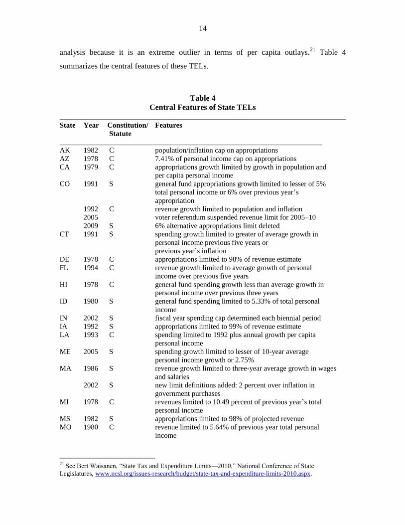
3. TELs in 30 States

Various forms of limits on revenues or spending have been imposed by 31 states. That

figure includes Alaska, which is shown in table 4 but excluded from the empirical

18

In present-value terms. See Alicia H. Munnell et. al., “The Funding of State and Local Pensions: 2011–

2015,” Center for Retirement Research at Boston College, monograph no. 24 (May 2012),

http://crr.bc.edu/wp-content/uploads/2012/05/slp_24.pdf. 19

Andrew G. Biggs, Public Sector Pensions: How Well Funded Are They, Really? State Budget Solutions,

July 2012, www.aei.org/files/2012/07/19/-biggs-state-budget-solutions-paper_125345809045.pdf. See also

Andrew G. Biggs, “An Options Pricing Method for Calculating the Market Price of Public Sector Pension

Liabilities,” Public Budgeting & Finance 31, no. 3 (Fall 2011): 94–118. 20

Biggs, Public Sector Pensions, 1.

14

analysis because it is an extreme outlier in terms of per capita outlays.21

Table 4

summarizes the central features of these TELs.

Table 4

Central Features of State TELs

________________________________________________________________________ State Year Constitution/ Features

Statute

________________________________________________________________________

AK 1982 C population/inflation cap on appropriations

AZ 1978 C 7.41% of personal income cap on appropriations

CA 1979 C appropriations growth limited by growth in population and

per capita personal income

CO 1991 S general fund appropriations growth limited to lesser of 5%

total personal income or 6% over previous year’s

appropriation

1992 C revenue growth limited to population and inflation

2005 voter referendum suspended revenue limit for 2005–10

2009 S 6% alternative appropriations limit deleted

CT 1991 S spending growth limited to greater of average growth in

personal income previous five years or

previous year’s inflation

DE 1978 C appropriations limited to 98% of revenue estimate

FL 1994 C revenue growth limited to average growth of personal

income over previous five years

HI 1978 C general fund spending growth less than average growth in

personal income over previous three years

ID 1980 S general fund spending limited to 5.33% of total personal

income

IN 2002 S fiscal year spending cap determined each biennial period

IA 1992 S appropriations limited to 99% of revenue estimate

LA 1993 C spending limited to 1992 plus annual growth per capita

personal income

ME 2005 S spending growth limited to lesser of 10-year average

personal income growth or 2.75%

MA 1986 S revenue growth limited to three-year average growth in wages

and salaries

2002 S new limit definitions added: 2 percent over inflation in

government purchases

MI 1978 C revenues limited to 10.49 percent of previous year’s total

personal income

MS 1982 S appropriations limited to 98% of projected revenue

MO 1980 C revenue limited to 5.64% of previous year total personal

income

21

See Bert Waisanen, “State Tax and Expenditure Limits—2010,” National Conference of State

Legislatures, www.ncsl.org/issues-research/budget/state-tax-and-expenditure-limits-2010.aspx.

15

1996 C voter approval required for tax increases the lesser of $77

million or 1% of state revenues

MT 1981 S spending limited to index of total personal income

2005 invalidated by state attorney general

NV 1979 S proposed spending limited to biennial population and

inflation growth

NJ 1990 S spending growth limited to growth in total personal income

NC 1991 S spending limited to 7% of total personal income

OH 2006 S spending limited to greater of 3.5% growth or inflation plus

population

OK 1985 C spending growth limited to 12% plus inflation

1985 C appropriations limited to 95% of certified revenue

OR 2000 C taxpayer refund of general fund revenues over 102% of

revenue estimate

2001 S appropriations growth limited to 8% of projected biennial

total personal income

RI 1992 C appropriations limited to 98% of projected revenue (97%

after July 1, 2012)

SC 1980 C spending growth limited to greater of average growth in

personal income or 9.5% total personal income in previous

year

TN 1978 C appropriations limited to growth total personal income

TX 1978 C biennial appropriations limited to growth total personal

income

UT 1989 S spending growth limited by population growth, inflation

WA 1993 S spending growth limited to inflation over previous three years

plus population growth

WI 2001 S spending growth on appropriations with some exceptions

limited to growth in total personal income

________________________________________________________________________

Sources: National Conference of State Legislatures, “State Tax and Expenditure Limits,” various

years, www.ncsl.org/home/search-results.aspx?zoom_query=spending%20limits; author

discussions with various state staffers; Michael J. New, “U.S. State Tax and Expenditure

Limitations: A Comparative Political Analysis,” State Politics and Policy Quarterly 10, no. 1

(Spring 2010): 25–50; Matthew Mitchell, “TEL It Like It Is: Do State Tax and Expenditure

Limits Actually Limit Spending?” Mercatus Center Working Paper No. 10-71, December 2010,

http://mercatus.org/sites/default/files/publication/TEL%20It%20Like%20It%20Is.Mitchell.12.6.1

0.pdf; and Sharon N. Kioko, “Structure of State-Level Tax and Expenditure Limits,” Public

Budgeting & Finance 31, no. 2 (Summer 2011): 43–78.

It is clear that the various state limits on spending or taxes or both display a wide

variety of definitions and adjustments, and implicit within these differences is a range of

opportunities to evade them.22

Accordingly, the various state efforts to impose fiscal

discipline through such tools offer a useful set of experiments with which to evaluate

their success. There exists a substantial literature on this topic, most of which omits

22

An example: a limit defined in terms of estimated (future) revenue would be easier to circumvent than a

similar one defined in terms of historical revenue, other things equal.

16

Alaska from empirical analyses because of its heavy dependence on severance taxes on

oil production. The existing empirical literature on the effects of TELs also largely treats

the adoption (or presence) of a TEL-type policy in a given state essentially as

predetermined (or exogenous)—that is, there has been little effort to examine the

question of why a state chooses to adopt a TEL.

Bails and Tieslau argue, somewhat unclearly, that TELs at the state and local

level are consistent with “the assumption that state and local governments are more

responsive to the needs of the citizenry.”23

They estimate an econometric model to

examine the effects of tax and expenditure limits and other fiscal policy constraints on the

growth in state and local spending, using a cross-section of 49 states observed at five-

year intervals from 1969 through 1994. They find that tax or expenditure limits have the

effect of creating a one-time reduction in state spending levels of about $78 per capita (in

2011 dollars).24

This is a reduction of about 2.5 percent.

New (2001) estimates an econometric model of the effect of TELs in which the

structure of a given TEL is affected by its political history: a fiscal constraint created by

the legislature can be predicted to prove less effective than one created by a citizen

initiative, in that the legislature is less likely to be interested in imposing effective

constraints upon itself.25

Of course, “citizen” initiatives might be promoted by groups

also interested in expanded spending—the public education lobby is a good example—

but New’s model, as with the rest of the existing literature, does not delve into the

endogenous nature of TELs, whether enacted by legislatures or by citizen initiatives.

New’s findings (in 2011 dollars) can be summarized as follows, based on a sample of

data from 49 states during 1972 through 1996:

A TEL enacted as a result of a citizen initiative reduces spending by about $27

per capita annually, or about 0.4 percent for the average state in 1996;

23

Dale Bails and Margie A. Tieslau, “The Impact of Fiscal Constitutions on State and Local Expenditures,”

Cato Journal 20, no. 2 (Fall 2000): 255–77, at 255. 24

In other words, spending is predicted to be lower by about $80 per person every year with a TEL than

without, other things equal. This is different from a given percentage reduction, which would yield a slower

growth rate in spending. 25

Michael J. New, “Limiting Government through Direct Democracy: The Case of State Tax and

Expenditure Limitations,” Cato Institute Policy Analysis No. 420, December 13, 2001,

www.cato.org/pubs/pas/pa420.pdf.

17

A TEL enacted by the legislature yields an increase in per capita spending by

about $23.50, or about 0.3 percent in 1996;

A “strong” TEL that limits spending growth to increases in inflation and

population reduces per capita spending by about $193, or about 2.8 percent in

1996;

A TEL not based on inflation and population but that mandates taxpayer refunds

of surplus revenues reduces per capita spending by about $67, or 1 percent in

1996; and

Other TELs have the effect of increasing per capita spending by about $24.50, or

about 0.4 percent in 1996.

Kousser, McCubbins, and Moule compare given states before and after

enactments of their respective TELs and against a control group of states without TELs,

during the period 1969–2000.26

They find that TELs are largely ineffective and can be

circumvented through the use of fees. The one exception is Colorado, for which they find

a reduction in per capita spending of about $430 (in 2011 dollars), or about 4.7 percent in

2000.27

The Colorado case is discussed in more detail in section 4.

In a more recent analysis, New (2010) confirms his earlier findings that TELs

enacted as a result of citizen initiatives are the most effective in terms of limiting total

spending, using data for 49 states from 1972 through 2000.28

That effect (in 2011 dollars)

is about $54 per capita, or about 0.7 percent in 2000 for the average state.29

For “strong”

26

Thad Kousser, Mathew D. McCubbins, and Ellen Moule, “For Whom the TEL Tolls: Can State Tax and

Expenditure Limits Effectively Reduce Spending?” State Politics and Policy Quarterly 8, no. 4 (Winter

2008): 331–61. 27

Total state and local spending in Colorado in 2000 was about $33.8 billion (in year 2011 dollars). For the

spending data, see “Comparison of State and Local Government Spending in the United States, Fiscal Year

2000,” www.usgovernmentspending.com/compare_state_spending_2000bF0a; US Census Bureau, “State

and Local Government Finances,” www.census.gov/govs/local/; and US Census Bureau, “Population

Estimates,” www.census.gov/popest/data/historical/2000s/vintage_2001/state.html. The population was

about 4.3 million, yielding total per capita spending of about $7,874. 28

New, “Limiting Government.” 29

For the average state, per capita outlays in 2000 were $7,482 in 2011 dollars. See Bureau of Economic

Analysis, “National Data,” www.bea.gov/iTable/index_nipa.cfm, tables 3.3 and 3.9.4; and US Census

Bureau, “Population Estimates.”

18

TELs limiting spending increases with a formula based on inflation and population

growth, the effect is over $150 per capita, or over 2 percent.30

Mitchell reports findings on the effects of TELs using data from 49 states for the

period 1977 through 2006.31

For state and local spending shares of total income, he finds

an overall downward effect of TELs defined in terms of inflation and population of about

0.6 percent relative to other states.32

Interestingly, Mitchell finds that TELs defined in

terms of income growth (rather than inflation and population) reduce state spending as a

share of income by about 0.4–0.8 percent in low-income states but that the effect of such

TELs in high-income states is an increase of about 0.2–0.6 percent.

In short, the existing literature finds that TELs have small effects at most. The

next section utilizes more recent data for a discussion of the respective state averages and

trends and for estimation of an econometric model of the effects of TELs.

4. Empirical Examination of the Effects of TELs

Table 5 presents a before/after comparison of per capita state and local spending and

spending growth rates for the 30 states (excluding Alaska) with some form of TEL in

effect during any part of the period 1970–2010. For each state, Table 5 presents the year

that the given TEL became effective, average per capita outlays before and during (and

after in a few cases in which the given TELs were discarded or weakened) the periods of

effectiveness, average growth rates in per capita outlays during and outside the periods of

effectiveness, the respective standard deviations, and whether or not the differences are

statistically significant.33

30

Note again that these reductions are downward shifts in the level of per capita spending, rather than a

reduction in the rate of spending growth. Accordingly, the percentage reductions are not compounded over

time. 31

Matthew Mitchell, “TEL It Like It Is: Do State Tax and Expenditure Limits Actually Limit Spending?”

Mercatus Center Working Paper No. 10-71, December 2010,

http://mercatus.org/sites/default/files/publication/TEL%20It%20Like%20It%20Is.Mitchell.12.6.10.pdf. 32

Ibid., 21. 33

Because the adoption of a TEL is endogenous—a choice variable—I use a two-tailed test for statistical

significance of the differences. It is possible, for example, that a given TEL might be adopted as a tool for

interest groups to achieve spending higher rather than lower. The significance levels are the standard 5

percent, that is, the confidence intervals are computed at a 95 percent level.

19

Table 5

Per Capita State and Local Outlays: Summary Data for 30 TEL States, 1970–2010 ______________________________________________________________________________

State TEL Avg. Outlays Std. Diff. Avg. Growth Std. Diff.

Years Before/After Dev. Stat. Before/After Dev. Stat. Sig?

Effective (2011 $) Sig? (%)

______________________________________________________________________________

AZ 1979+ 4,659/6,317 272 yes 2.3/1.1 3.3 no

CA 1980– 5,853/6,291 203 yes 0.7/1.7 3.5 no

1990 6,291/8,828 581 yes 1.7/1.4 3.9 no

CO 1994– 5,518/7,856 770 yes 2.4/0.6 3.6 no

2005 7,856/7,982 598 no 0.6/1.5 4.5 no

CT 1991+ 5,473/9,231 1,047 yes 2.8/0.8 3.8 no

DE 1979+ 5,628/8,089 267 yes 0.7/1.8 6.4 no

FL 1995+ 4,781/7,588 965 yes 2.8/0.6 3.9 no

HI 1979+ 7,098/8,216 305 yes 0.2/0.9 4.7 no

ID 1980+ 4,296/5,907 278 yes 1.3/1.4 3.9 no

IN 2002+ 4,935/7,490 1,286 marginal 2.5/–0.3 3.4 no

IA 1992+ 5,084/7,868 589 yes 1.9/1.8 3.1 no

LA 1993+ 5,077/7,960 744 yes 2.8/2.2 4.3 no

ME 2005+ 5,940/8,790 1,755 no 2.2/−1.0 3.1 no

MA 1986+ 5,356/8,462 270 yes 1.4/2.1 3.3 no

MI 1979+ 5,205/7,155 367 yes 2.6/1.1 3.0 no

MS 1983+ 3,943/6,344 248 yes 1.5/2.5 3.3 no

MO 1980+ 3,789/5,704 105 yes 0.7/2.1 3.9 no

1996+ 4,275/6,904 632 yes 1.8/1.6 3.6 no

MT 1981– 5,094/6,759 475 yes 2.0/1.5 5.2 no

2005 6,759/7,886 899 no 1.5/1.1 2.8 no

NV 1980+ 5,954/7,073 159 yes 0.7/0.5 3.7 no

NJ 1990+ 5,441/8,986 821 yes 3.2/1.4 3.4 no

NC 1991+ 4,004/7,032 549 yes 2.6/1.7 3.5 no

OH 2007+ 5,790/8,118 1,625 no 2.4/−0.7 2.4 no

OK 1986+ 4,200/6,181 283 yes 1.4/1.8 2.9 no

OR 2001+ 6,421/8,524 1,216 no 2.2/−0.3 3.4 no

RI 1992+ 5,508/8,500 934 yes 2.9/0.7 2.6 no

SC 1980+ 3,677/6,333 1,650 no 3.0/2.3 3.9 no

TN 1978+ 3,715/5,623 218 yes 2.5/1.7 3.3 no

TX 1978+ 3,724/5,981 236 yes 2.5/2.0 4.2 no

UT 1989+ 4,815/7,055 456 yes 1.3/1.5 4.0 no

WA 1996– 6,099/8,595 1,043 yes 2.1/0.5 4.8 no

2000 8,595/8,903 249 no 0.5/0.4 3.2 no

WI 2001+ 6,273/8,503 1,218 marginal 2.1/−0.3 2.6 no

______________________________________________________________________________

Sources: See US Census Bureau, “State and Local Government Finances,”

www.census.gov/govs/local/; and US Census Bureau, “Population Estimates,”

www.census.gov/popest/data/historical/2000s/vintage_2001/state.html; and author’s

computations.

20

In terms of a simple statistical test of the effect of TELs on average real per capita

outlays or the growth of real per capita outlays, the appropriate null hypothesis is that

those spending variables remain unchanged as a matter of statistical significance during

periods when the TELs are in effect relative to the periods when the TELs are not in

effect. In other words, the central question here is whether TELs can be shown to impose

some degree of enhanced fiscal discipline—that is, a reduction in outlays or the growth of

outlays. The effectiveness of TELs must be demonstrated as a matter of statistical (and

economic) significance; accordingly, the null hypothesis appropriately is that they do not

make a difference.

The summary data presented in table 5 do not distinguish among the differing

features of the TELs adopted by the respective states, nor do they control for the crucial

factors (variables) that drive spending outcomes as determined in political processes.34

Accordingly, these summary data are not conclusive; but they are highly suggestive. For

average per capita outlays, 23 of the 30 states show a statistically significant increase

during periods when their respective TELs were in effect. For three of the states

(Colorado, Montana, and Washington), the evidence is mixed, but in none of those three

did outlays decline during the periods when the TELs were effective. In two states

(Indiana and Wisconsin), the statistical significance of the increases in per capita outlays

is marginal, and in the remaining four states (Maine, Ohio, Oregon, and South Carolina),

the increases in per capita spending were not statistically significant.

In terms of the growth rates of per capita outlays, 20 of the 30 states display a

decline in that growth rate during the periods when the respective TELs were effective,

but none of those differences is statistically significant. Three of the states (California,

Colorado, and Missouri) show a mixed record, but, again, none of the changes in growth

rates is statistically significant. Seven of the states (Delaware, Hawaii, Idaho,

Massachusetts, Mississippi, Oklahoma, and Utah) displayed higher growth rates during

the TEL periods, but, yet again, the increases were not statistically significant.

Note that a majority of the states displayed a decline in their respective growth

rates for per capita outlays during the TEL periods, but even apart from the absence of

34

Because the comparisons in table 5 are between time periods rather than between states, some of those

variables implicitly are held constant, as some such factors are specific to particular states rather than

particular time periods.

21

statistical significance, the declining growth rates may be driven in substantial part by the

universal pattern of higher absolute levels of per capita spending as we move from the

earlier years to the later ones: any given amount of increased spending is a lower

percentage of a higher base amount.

Table 6 presents the respective averages and standard deviations for per capita

outlays and growth rates in per capita outlays for states with and without TELs, for the

period 1970–2010. Note that in our sample, the earliest TELs became effective in 1978

(in Tennessee and Texas). Again, Alaska is excluded from the sample.

Table 6

Average Per Capita Outlays and Outlay Growth, TEL and Non-TEL States ______________________________________________________________________________

Year TEL Avg. Non-TEL Std. Avg. TEL Std. Avg. Non-TEL Std. Avg. TEL Std.

States Outlays Dev. Outlays Dev. Growth Dev. Growth Dev.

(2011 $) (2011 $) (%) (%)

______________________________________________________________________________

1970 0 4,255 831 na na na na na na

1971 0 4,457 870 na na 4.8 3.3 na na

1972 0 4,556 911 na na 2.2 3.1 na na

1973 0 4,586 879 na na 0.8 2.5 na na

1974 0 4,449 833 na na −2.9 2.1 na na

1975 0 4,690 837 na na 5.6 3.3 na na

1976 0 4,915 880 na na 4.9 3.8 na na

1977 0 4,911 863 na na 0.0 2.8 na na

1978 2 4,991 830 4,130 61 0.9 3.2 3.5 0.7

1979 6 5,016 787 5,236 965 1.8 2.6 0.1 3.7

1980 11 4,955 766 4,820 942 −1.1 1.9 −3.2 2.5

1981 12 4,950 828 4,892 944 0.1 3.2 0.3 3.0

1982 12 5,006 991 4,829 1,023 0.8 4.6 −0.7 3.5

1983 13 5,032 999 4,724 998 0.1 2.6 −1.0 4.1

1984 13 5,173 1,066 4,847 980 2.7 2.4 2.5 3.4

1985 13 5,394 1,080 5,045 941 4.1 2.7 3.7 3.3

1986 15 5,628 1,124 5,342 911 4.3 2.5 5.8 2.1

1987 15 5,742 1,083 5,384 926 2.2 3.5 1.1 3.7

1988 15 5,865 1,047 5,572 1,002 2.3 3.3 3.9 4.2

1989 16 6,131 1,077 5,779 996 4.3 1.4 3.6 2.4

1990 17 6,278 1,077 6,046 1,088 3.1 1.4 2.5 2.4

1991 18 6,588 1,087 6,300 1,202 4.6 1.4 4.2 2.4

1992 20 6,919 1,145 6,736 1,314 5.5 1.5 5.3 2.3

1993 21 7,071 1,132 6,834 1,256 2.3 3.5 1.3 2.2

1994 22 7,115 1,137 7,008 1,212 0.9 3.9 2.4 3.7

1995 23 7,328 1,155 7,193 1,141 3.0 4.4 2.7 3.4

1996 24 7,350 1,111 7,284 1,028 1.0 2.1 0.4 2.5

1997 24 7,621 1,114 7,512 936 3.8 2.6 3.2 3.3

1998 24 7,797 1,119 7,655 900 2.4 2.9 1.6 2.5

22

1999 24 7,942 1,137 7,811 873 1.9 1.9 2.1 1.9

2000 24 7,987 1,112 7,673 918 0.6 2.6 −1.3 3.1

2001 25 8,257 1,159 8,056 906 3.9 1.6 4.3 2.4

2002 26 8,663 1,230 8,412 906 4.4 1.4 4.7 2.0

2003 26 8,650 1,262 8,272 892 −0.2 2.4 −1.8 2.6

2004 26 8,636 1,322 8,141 936 −0.2 2.2 −1.8 2.5

2005 27 8,468 1,475 8,054 942 −1.7 3.3 −1.2 3.0

2006 25 8,365 1,413 8,066 1,051 −0.6 2.1 −0.1 2.2

2007 26 8,355 1,582 7,993 931 −0.2 4.6 −0.7 4.3

2008 26 8,370 1,707 7,985 999 0.0 2.5 0.1 3.9

2009 26 8,756 1,532 8,298 1,027 5.0 3.9 3.9 2.5

2010 26 8,741 1,505 8,101 1,002 −0.1 3.6 −2.7 3.5

______________________________________________________________________________

Note: “na” means not applicable or not available.

Sources: See US Census Bureau, “State and Local Government Finances,”

www.census.gov//govs/estimate/; and US Census Bureau, “Population Estimates,”

www.census.gov/popest/data/historical/2000s/vintage_2001/state.html; and author’s

computations.

The data presented in table 6 can be summarized as follows. In the sample of 49

states over the 41-year period 1970–2010, the first TELs became effective in 1978 in

Tennessee and Texas. The number of states with TELs grew over time to 27 in 2005, then

fell to 25 in 2006, and increased to 26 thereafter. In terms of average per capita state and

local outlays for the period 1978–2010, states without TELs spent more than states with

them in every year except 1979, but the differences are not statistically significant in any

year.35

Indeed, with the appropriate null hypothesis—per capita outlays in TEL states do

not differ from those in non-TEL states—the differences between the states with and

without TELs are far less than one standard deviation, with the exception of 1978, when

only two states had TELs in place.36

Even if we apply the opposite null hypothesis—that

per capita outlays in TEL states are lower than those in non-TEL states—the difference is

statistically significant only in 1978, again when there were only two states with TELs. In

every year thereafter, the differences between the TEL and non-TEL states again are far

smaller than one standard deviation.

In terms of the comparative growth rate data reported in table 6, the interpretation

problem noted above remains: growth rates will tend to be lower in states with higher per

35

As above, I use a 5 percent significance level. See note 33. 36

This finding is not due to a small number of states without TELs: the lowest number was in 2005, when

there were 22 such states out of 49 (excluding Alaska).

23

capita outlays. Putting that aside, for the 33 years between 1978 and 2010, states without

TELs had higher growth rates in per capita outlays in 22 years, while the TEL states had

higher growth rates in 11. Again, the differences in growth rates are not statistically

significant in any year.

Consider figure 1, which shows a plot of per capita state and local outlays for

Colorado for the period 1970–2010, along with the same data for all non-TEL states in

each respective year. The Colorado case is interesting because its TEL—the Taxpayer

Bill of Rights, or TABOR—is cited in some of the literature as a relatively successful

constraint on the growth of government spending, at least for a temporary period.37

As a

practical matter, the Colorado TEL was in effect for the period 1994–2005, and indeed

real per capita outlays declined during 1994 through 1996 but then increased from 1997

through 2002.38

Outlays declined sharply during 2002 through about 2008 and then

increased thereafter, unquestionably as a result of the federal economic recovery

legislation passed in 2009.

Relative to the pattern exhibited by the non-TEL states, these data do not suggest

an obvious difference engendered by the Colorado TEL, except that Colorado outlays

seem to have declined more sharply than was the case for the non-TEL states after 2002

(when the Colorado TEL still was in effect), reverting to approximately flat per capita

outlays until the increase beginning in 2009, a pattern mirrored by the non-TEL states.

Colorado per capita outlays fell below the non-TEL states’ figures after 2002, but the

TEL itself—again, in effect during 1994–2005—does not appear to have had a clear

relative effect, at least as revealed by these aggregate data. The change in growth rates, as

shown in table 5, was not statistically significant, and the econometric findings for

Colorado, as shown in tables 8 and 11, do not show a statistically significant effect of its

TEL.

37

See, for example, Michael J. New and Stephen Slivinski, “Dispelling the Myths: The Truth about

TABOR and Referendum C,” Cato Institute Briefing Paper No. 95, October 24, 2005; and New, “Limiting

Government,” table 4. 38

For a history of the Colorado TABOR, see New, “Limiting Government.”

24

Figure 1

Sources: Statistical Abstracts of the United States 1951–1994

(www.census.gov/popest/data/historical/index.html), and later years (www.census.gov/govs/local/); data

from the Bureau of Economic Analysis (www.bea.gov/iTable/iTable.cfm?ReqID=9&step=1), various

tables; and author computations.

Figures 2 through 5 for Arizona, South Carolina, Washington, and Tennessee are

discussed below. Appendix A presents similar figures for each of the other 25 states

(excluding Alaska) that had TELs in effect for any part of the period 1970–2010, as

summarized in table 5.

The summary data presented in tables 5 and 6, figures 1 through 5, and in the

figures shown in appendix A suggest at most that state TELs do not offer a reliable tool

with which to impose spending discipline upon states and localities. But these data cannot

be viewed as conclusive because they do not control for factors that are important

determinants of state and local spending other than the presence or absence of a TEL.

Instead, an econometric approach that controls for other important factors is required.

The existing econometric literature summarized in section 3 is important, and as a crude

generalization reports that TELs have effects that are small or nonexistent. But that

literature suffers from two important problems.

First, much of the existing literature has treated the presence or absence of a TEL

in a given state as “exogenous”—that is, the models have not attempted to analyze the

issue of why TELs are adopted (or not adopted) in the first place. (Some of the literature,

0

2000

4000

6000

8000

10000

19

70

19

72

19

74

19

76

19

78

19

80

19

82

19

84

19

86

19

88

19

90

19

92

19

94

19

96

19

98

20

00

20

02

20

04

20

06

20

08

20

10

Year 2011 Dollars

Year (TEL Effective 1994-2005)

Colorado: Per Capita Outlays

CO Per Capita Outlays Non-TEL Per Capita Outlays

25

however, has attempted to estimate the effects of TELs with different characteristics.)

Accordingly, the existence or absence of a TEL simply has been included as a variable

helping to explain (or predict) state and local spending, and the econometric analyses

then have generated estimates of the marginal effect of the TELs in terms of outlays per

capita or other dependent variables. This implicit exogeneity assumption is problematic

because it ignores one important possibility: that states with relatively high outlays adopt

TELs as a tool with which to achieve stronger fiscal discipline; in this case the data

analysis might yield an erroneous conclusion that the TELs have the effect of increasing

spending.39

A simple example of this “endogeneity” problem is as follows: Consider a police

force that assigns heavier patrol duty in high-crime areas. In the absence of an equation

predicting those patrolling decisions, a simple econometric model explaining crime rates

as a function of the intensity of patrols (and other variables) is likely to predict that more

police patrols are a cause of crime, because the econometric model will encounter a

strong positive correlation between crime and police patrols, and the remaining variables

controlling for the other factors that drive crime rates are unlikely to control for the

decision making of the police departments.40

Because the adoption of a TEL is a policy

choice, an appropriate econometric analysis should treat the adoption of a TEL as

endogenous, and a multiequation econometric approach (two-stage least squares) should

be used.41

That is the estimation technique used here.

Second, the existing literature tends largely to employ the relevant data in various

ratios: spending per capita or per unit of personal income, population subgroups as a

percentage of total population, unemployment rates, and the like. With respect to the

39

See the data on outlays and the associated standard deviations in table 5. Another possibility is that

concentrated interest groups in favor of higher spending design specific TELs so that greater spending

results. 40

Another simple example would be an analysis of the effect of an insecticide on farmland infestations.

Because farmers are likely to use insecticides more intensively on acres with greater infestations, a simple

econometric model analyzing the effect of the insecticide on infestations is likely to find that the insecticide

is healthy for the insects. The behavior of the farmers must be included in the model. 41

An additional question is why a TEL in a given state has the particular characteristics that it does. See

table 4. That is a complex question shunted aside in the analysis here. As an aside, because in the

econometric estimates for each individual state (discussed later in this section) the error terms are likely to

be correlated, an increase in the efficiency of the estimates might be achieved through the use of the three-

stage least squares estimator. That minor complication is ignored here, in part because of the large number

of observations for each state and for the sample as a whole.

26

spending data in particular, these formulations assume implicitly that spending rises

proportionately (linear homogeneity) with population or personal income, a constraint

that is likely to be incorrect for some public spending programs characterized by a

nontrivial degree of “publicness.”42

That means, crudely, that the given program yields

benefits that accrue to the population generally, or at least not merely to a given

consumer. National defense is the usual example of such a public (or collective) good at

the federal level. At the state and local level, policing services are a good example; the

consumption of an apple is an example of a good characterized by zero publicness. In the

estimates reported in tables 7–11, the data analysis is conducted in levels (for example,

total outlays), with the levels of population, economic variables, and the like included as

explanatory variables.

The two-stage model reported here is estimated first with cross-sectional and time

series data for 49 states for the period 1970–2010.43

For a given state in a given year,

total state and local outlays (direct general expenditures44

) are assumed to be determined

by the following variables:

42

Suppose that outlays O are determined by some set of variables Z and population: O = f(Z,pop). That

equation is homogeneous of degree k in population if λkO = f(Z,λpop). If λ = 1/pop, then O/pop

k = f(Z,1) =

g(Z). Accordingly, the use of outlays per capita assumes that k = 1. 43

In accordance with standard practice, the results of the first-stage analysis—the prediction of the

adoption or nonadoption of a TEL by a given state—are not reported separately here because the statistical

consistency of the second-stage estimates of interest does not depend on the consistency of the first stage.

Only the statistical independence of the TEL variable is needed, and the use of the predicted TEL variable

produced in the first-stage estimation process satisfies that condition. See Harry H. Kelejian, “Two-Stage

Least Squares and Econometric Systems Linear in Parameters but Nonlinear in the Endogenous Variables,”

Journal of the American Statistical Association 66, no. 334 (June 1971): 373–74. The variables used in the

first-stage equation to predict the adoption or nonadoption of a TEL are as follows: the five-year compound

spending growth rate lagged one year, total outlays lagged one year, state gross product lagged one year,

the five-year compound growth rate in population, total population, the state poverty rate, a zero-one

(“dummy”) variable denoting whether the governor is a Republican, a dummy variable denoting whether

the upper legislative chamber is controlled by the Republicans, a dummy variable denoting whether the

lower legislative chamber is controlled by the Republicans (for Nebraska, the unicameral legislature is

treated as having two houses controlled by the same party as the governor), a dummy variable denoted

whether the given state’s TEL was enacted by popular vote, a dummy variable denoting whether the given

state’s TEL is constitutional as distinct from statutory, and a dummy variable denoting whether the given

state’s TEL is defined in terms of some measure of state income or output as distinct from such other

parameters as inflation and population growth. For purposes of the two-stage econometric analysis, the

three TEL characteristics variables are treated as predetermined. 44

The data on direct general expenditures are reported by the US Census Bureau, “State and Local

Government Finances,” and US Census Bureau, “Statistical Abstracts 1951–1994,”

www.census.gov/prod/www/abs/statab1951-1994.htm; and US Department of Commerce—Bureau of

Economic Analysis, “National Income and Product Accounts Tables,”

www.bea.gov/iTable/iTable.cfm?ReqID=9&step=1.

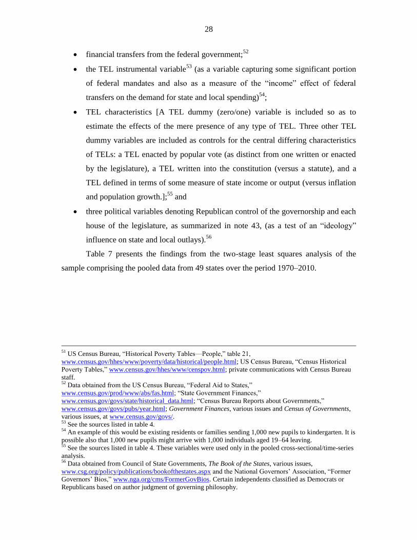
27

total state and local outlays lagged one year (because government budgeting is an

incremental process of decision making with respect to changes in outlays from

the previous year);

state gross product (as a proxy for the size of the tax base);45

total personal income (as one measure of the demand for public or publicly

provided services);46

total population (as another measure of demand conditions and also to control for

possible scale effects (either “publicness” or scale economies) in the provision of

public services);47

population aged 5–18 (as a proxy for the demand for K–12 education);48

population aged 65 and over (as a proxy for the demand for various other services

demanded disproportionately by retirees);49

total unemployment (as a proxy for unemployment insurance and other services

provided those looking for work, and also as a possible proxy variable for income

and sales tax revenues);50

population with incomes below the federal poverty level (as another proxy for

particular classes of programs financed by many states and localities);51

45

US Department of Commerce—Bureau of Economic Analysis, “GDP and Personal Income,”

www.bea.gov/iTable/iTable.cfm?ReqID=70&step=1&isuri=1&acrdn=1. 46

Ibid. 47

US Census Bureau, “Population Estimates—Pre-1980: State Tables,”

www.census.gov/popest/data/historical/pre-1980/state.html; “Intercensal Estimates of the Total Resident

Population of States: 1970 to 1980,” www.census.gov/popest/data/state/asrh/1980s/tables/st7080ts.txt;

“Intercensal Estimates of the Total Resident Population of States: 1980 to 1990,”

www.census.gov/popest/data/state/asrh/1980s/tables/st8090ts.txt; “State Population Estimates: Annual

Time Series, July 1, 1990 to July 1, 1999,” www.census.gov/popest/data/state/totals/1990s/tables/ST-99-

03.txt; “Population Estimates: Historical Data: 2000s,”

www.census.gov/popest/data/historical/2000s/index.html; and “State Totals: Vintage 2011,”

www.census.gov/popest/data/state/totals/2011/index.html. 48 Data obtained from the US Census Bureau, “Population Estimates: Historical Data,”

www.census.gov/popest/data/historical/index.html; “Population Estimates, Pre-1980: State Tables,”

www.census.gov/popest/data/historical/pre-1980/state.html; “State Population Estimates and Demographic

Components of Change: 1980 to 1990, by Single Year of Age and Sex,”

www.census.gov/popest/data/state/asrh/1980s/80s_st_age_sex.html; “Population Estimates for the US,

Regions, and States by Selected Age Groups and Sex: Annual Time Series, July 1, 1990, to July 1, 1999,”

www.census.gov/popest/data/state/asrh/1990s/tables/ST-99-09.txt; the respective state tables at

“Population Estimates—Historical Data: 2000s,” www.census.gov/popest/data/historical/2000s/index.html;

and private communications with Census Bureau staff. 49

Ibid. 50

US Bureau of Labor Statistics, “Civilian Labor Force,” www.bls.gov/lau/staadata.txt; and private

communications with BLS staff.

28

financial transfers from the federal government;52

the TEL instrumental variable53

(as a variable capturing some significant portion

of federal mandates and also as a measure of the “income” effect of federal

transfers on the demand for state and local spending)54

;

TEL characteristics [A TEL dummy (zero/one) variable is included so as to

estimate the effects of the mere presence of any type of TEL. Three other TEL

dummy variables are included as controls for the central differing characteristics

of TELs: a TEL enacted by popular vote (as distinct from one written or enacted

by the legislature), a TEL written into the constitution (versus a statute), and a

TEL defined in terms of some measure of state income or output (versus inflation

and population growth.];55

and

three political variables denoting Republican control of the governorship and each

house of the legislature, as summarized in note 43, (as a test of an “ideology”

influence on state and local outlays).56

Table 7 presents the findings from the two-stage least squares analysis of the

sample comprising the pooled data from 49 states over the period 1970–2010.

51

US Census Bureau, “Historical Poverty Tables—People,” table 21,

www.census.gov/hhes/www/poverty/data/historical/people.html; US Census Bureau, “Census Historical

Poverty Tables,” www.census.gov/hhes/www/censpov.html; private communications with Census Bureau

staff. 52

Data obtained from the US Census Bureau, “Federal Aid to States,”

www.census.gov/prod/www/abs/fas.html; “State Government Finances,”

www.census.gov/govs/state/historical_data.html; “Census Bureau Reports about Governments,”

www.census.gov/govs/pubs/year.html; Government Finances, various issues and Census of Governments,

various issues, at www.census.gov/govs/. 53

See the sources listed in table 4. 54

An example of this would be existing residents or families sending 1,000 new pupils to kindergarten. It is

possible also that 1,000 new pupils might arrive with 1,000 individuals aged 19–64 leaving. 55

See the sources listed in table 4. These variables were used only in the pooled cross-sectional/time-series

analysis. 56

Data obtained from Council of State Governments, The Book of the States, various issues,

www.csg.org/policy/publications/bookofthestates.aspx and the National Governors’ Association, “Former

Governors’ Bios,” www.nga.org/cms/FormerGovBios. Certain independents classified as Democrats or

Republicans based on author judgment of governing philosophy.

29

Table 7

Econometric Findings: Pooled Sample

(dependent variable: total state and local outlays in 2011 dollars) ______________________________________________________________________________

Variable Estimated Coefficient T-Statistic

______________________________________________________________________________

Outlays lagged 0.87 70.92

State gross product −0.01 −3.88

Total personal income 0.03 11.40

Population 0.51 2.06

Population 5–18 2.17 3.45

Population 65+ −1.35 −2.57

Total unemployed −2.78 −3.41

Poverty population 1.41 4.89

Federal transfers 0.18 5.39

TEL 2,135.48 0.41

TEL popular vote −190.22 −0.94

TEL constitution −856.01 −1.19

TEL income/output −1,481.64 −1.40

Republican governor −282.48 −2.79

Republican lower leg. house −65.91 −0.55

Republican upper leg. house 36.41 0.32

constant −265.60 −1.47

pseudo adj. R2 0.999

______________________________________________________________________________

Source: Author’s computations.

Other factors held constant, an increase in outlays of $1 million during the

previous year results in an increase in current-year outlays of about $870,000; this is

consistent with the incremental nature of government budgeting. The size of the tax base

as measured by state gross product is significant statistically but has an unexpected

negative sign; the coefficient (−0.01) is so small that the variable effectively is irrelevant

economically. An increase in total personal income has a very small but statistically

significant effect on total outlays. An increase in total population of 1,000—holding

constant the school-age and retiree populations—results in greater outlays of about

$510,000. An increase in the school-age population of 1,000, holding constant the total

and retiree populations, is predicted to increase total outlays by about $2.2 million.57

An

57

Obviously, taxes paid to the federal government by state residents have the effect of reducing such

demands, but they in effect are predetermined in the federal tax code; moreover, the deductibility of state

30

increase of 1,000 in the population aged 65 and above, holding the other population

variables constant (that is, replacing 1,000 individuals aged 19–64), reduces spending by

about $1.4 million. This effect is likely to result from a decrease in the income tax base

attendant upon such a population shift of 1,000 retirees in place of 1,000 individuals aged

19–64, even though state gross product is included as a proxy for the tax base. If 1,000

retirees replace 1,000 students, the net effect is a reduction in outlays of about $3.5

million (that is, the sum of the coefficients, or [−2.17 + −1.35]). An increase in total

unemployment of 1,000 results in decline in outlays of about $2.8 million; unemployment

in this model is likely to be serving as a proxy variable for tax revenues, although, again,

state gross product should serve that function in this model. An increase of 1,000 in the

population of poor individuals (holding unemployment constant) increases spending by

about $1.4 million. An increase in federal financial transfers of $1 million, other factors

held constant, increases state and local outlays on net by only $180,000. It is likely to be

the case that such federal transfer programs—Medicaid may be a good example—force

state and local spending upward on particular programs, with reductions in others.

Moreover, the average state must pay an increase in current or future federal taxes equal

to the increase in federal transfers received.

Those variables are statistically significant at levels lower or far lower than a 5

percent significance level (or higher than a 95 percent confidence interval). The presence

of a TEL is associated with an increase in outlays of about $2.1 billion; but the variable

fails the test for statistical significance. A TEL enacted by popular vote has a coefficient

smaller in absolute value—reduced outlays over $190 million—but does not differ from

zero as a matter of statistical significance. The same is true for a TEL enacted as a part of

the constitution: it is not statistically significant. A TEL defined as some function of

incomes or state output has a coefficient larger in absolute value but again is not

statistically significant.

The presence of a Republican governor is predicted to reduce outlays by about

$282 million for the average state. Republican control of neither the upper nor lower

house of the legislature has an effect that is statistically significant.

and local taxes from the federal income tax base offsets that effect to some degree. This is a complication

ignored here.

31

Table 8 presents the estimated TEL coefficients for each of the 30 TEL states,

estimated separately.58

Among the 30 TEL states, only nine have estimated coefficients

for the TEL variable greater than the respective standard errors (a T statistic greater than

1 in absolute value). Of those estimated coefficients, only four are statistically significant

at an approximate significance level of 10 percent or lower (a confidence interval of 90

percent or higher) and of those, one (Massachusetts) is positive, implying that its TEL

had the effect of (or was written so as to) driving outlays upward.59

The other three states

are Arizona, South Carolina, and Washington; table 9 summarizes the econometric

evidence on the effect of their respective TELs.

Table 8

TEL Effects for 30 States: State and Local Outlays ______________________________________________________________________________

State TEL Coefficient T-Statistic

______________________________________________________________________________

Arizona −1,167.1 −1.80

California −5,761.9 −1.18

Colorado −169.7 −0.25

Connecticut 1,248.8 1.38

Delaware 17.9 0.06

Florida −2,855.0 −0.94

Hawaii −91.3 −0.15

Idaho −349.1 −0.81

Indiana 452.4 0.33

Iowa 2,379.9 0.49

Louisiana −359.0 −0.25

Maine 90.3 0.58

Massachusetts 2,262.6 1.86

Michigan −2,885.5 −1.19

Mississippi −262.8 −0.26

Missouri −849.4 −0.65

Montana −10.6 −0.09

Nevada 2,768.7 1.24

New Jersey 2,607.8 1.02

North Carolina 270.5 0.22

Ohio 7,122.3 0.40

Oklahoma 1,057.5 0.80

Oregon 278.4 0.48

58

The estimated equations for each of the 30 TEL states are available from the author upon request. The

TEL characteristics variables were excluded from the individual state regressions because virtually none of

them varied in a given state over the sample period 1970–2010. 59

This is not counterintuitive. A given TEL can be advertised as a tool for fiscal restraint while written so

as to further the preferences of concentrated interest groups for higher spending.

32

Rhode Island 247.7 1.04

South Carolina −1,636.9 −1.94

Tennessee −548.6 −0.63

Texas 343.5 0.10

Utah 1,202.3 0.91

Washington −2,436.4 −1.96

Wisconsin 170.5 0.20

______________________________________________________________________________

Source: Author’s estimates and computations.

Table 9

Estimated Effect of TELs in Arizona, South Carolina, and Washington ______________________________________________________________________________

State TEL Estimated Annual Outlay Average Outlays TEL Effect

(Years) Coefficient Effecta TEL (Years)

a (%)

_____________________________________________________________________________

Arizona 1979–2010 −1,167.1 −1.2 28.9 4.2

South Carolina 1980–2010 −1,636.9 −1.6 24.6 6.5

Washington 1996–2000 −2,436.4 −2.4 49.0 4.9

______________________________________________________________________________ Note:

a Billions of 2011 dollars.

Source: Author’s estimates and computations.

Figures 2 through 4 display the per capita spending paths for these three states.

33

Figure 2

Sources: Statistical Abstracts of the United States 1951–1994

(www.census.gov/popest/data/historical/index.html), and later years (www.census.gov/govs/local/); data

from the Bureau of Economic Analysis (www.bea.gov/iTable/iTable.cfm?ReqID=9&step=1), various

tables; and author computations.

The Arizona TEL became effective in 1979, and per capita outlays fell that year

both absolutely and relative to average per capita outlays in states without TELs. But per

capita spending growth in Arizona exceeded that for the latter group of states beginning

in 1984, flattening after 1988. More broadly, per capita outlays in Arizona after 1990

have been lower than those for non-TEL states, a pattern confirmed by the econometric

estimates on total outlays, as presented in table 8. For 1970–90, the ratio of per capita

outlays in the non-TEL states to those for Arizona ranged from about 0.97 to about 1.05,

with an average of 0.99. For 1991–2010, that ratio ranged from 1.03 to 1.26, with an

average of 1.17. Accordingly, there seems to have been a downward spending shift

relative to the non-TEL states beginning around 1990, as illustrated in figure 2; but it is

problematic to ascribe that change to the Arizona TEL implemented in 1979.

For South Carolina (figure 3), the TEL became effective in 1980, and per capita

outlays fell below the 1981 figure until 1985. Growth in per capita outlays for South

Carolina since 1984 has been higher than that for the non-TEL states, and the absolute

0

1000

2000

3000

4000

5000

6000

7000

8000

9000

10000

19

70

19

72

19

74

19

76

19

78

19

80

19

82

19

84

19

86

19

88

19

90

19

92

19

94

19

96

19

98

20

00

20

02

20

04

20

06

20

08

20

10

Year2011 Dollars

Year (TEL Effective 1979–2010)

Arizona: Per Capita Outlays

AZ Per Capita Outlays Non-TEL Per Capita Outlays

34

difference in the respective outlay figures over time has narrowed in the period after 1984

relative to the 1970–84 period. For 1970–80, the ratio of non-TEL to South Carolina per

capita outlays was 1.28; for 1970–84, it was 1.29. For 1980–84, it was 1.30, and for

1985–2010, it was 1.11. Accordingly, that ratio has declined during the TEL period: the

crude data suggest that the South Carolina TEL may not have had a large effect given that

South Carolina per capita outlays have been lower than those for the non-TEL states

every year but have grown relative to the latter in the period during which the TEL has

been effective. Nonetheless, the econometric finding is that the South Carolina TEL has

yielded a decline in total state and local outlays of about $1.6 billion per year, statistically

significant at about a 5 percent significance level.

Figure 3

Sources: Statistical Abstracts of the United States 1951–1994

(www.census.gov/popest/data/historical/index.html), and later years (www.census.gov/govs/local/); data

from the Bureau of Economic Analysis (www.bea.gov/iTable/iTable.cfm?ReqID=9&step=1), various

tables; and author computations.

The most interesting case is the Washington TEL (figure 4), passed by the voters

in 1993 and which took effect in 1996 and then was amended in 2000 by the state

legislature in a way that created a large loophole that substantially weakened it. The TEL

limited increases in state outlays to the sum of the inflation and population growth rates.60

60

The TEL also reduced the spending limit when functions funded by general revenues were shifted to

local governments, thus preventing the legislature from evading the limit through such shifts.

0

2000

4000

6000

8000

10000

Year 2011 Dollars

Year (TEL Effective 1980–2010)

South Carolina: Per Capita Outlays

SC Per Capita Outlays Non-TEL Per Capita Outlays

35

Between 1997 and 2000, per capita outlays declined by about 1 percent, but then

increased by almost 10 percent in the two years after 2000. Per capita outlays fell relative

to those for the non-TEL states over 1996–2000 and absolutely in 2000 by about 3

percent. The pattern for per capita outlays roughly follows that for the non-TEL states

after 2000, although the decline for Washington was sharper during 2002–06. The

econometric finding here is that the Washington TEL engendered a decline in total state

and local outlays of about $2.4 billion per year, statistically significant at about a 5

percent significance level.

Figure 4

Sources: Statistical Abstracts of the United States 1951–1994

(www.census.gov/popest/data/historical/index.html), and later years (www.census.gov/govs/local/); data

from the Bureau of Economic Analysis (www.bea.gov/iTable/iTable.cfm?ReqID=9&step=1), various

tables; and author computations.

In the face of pressures from spending interests, the Washington state legislature

in 2000 amended the TEL by allowing the limit to rise when functions funded by special

accounts were shifted into the general fund. This act created a significant loophole: the

legislature was able to increase the spending limit by shifting special accounts into and

0

2000

4000

6000

8000

10000

Year 2011 Dollars

Year (TEL Effective 1996–2000)

Washington: Per Capita Outlays

WA Per Capita Outlays Non-TEL Per Capita Outlays

36

then out of the general fund. The state supreme court subsequently ruled this

circumvention to be legal.61

This experience in Washington may be instructive: to the (highly limited) extent

that spending limits prove effective, they are likely to be subject to erosion driven by the

same political factors that yield the fiscal pressures discussed in section 2. Among these

factors is the presence of concentrated interest groups with incentives to use political

processes to weaken TELs or other tools proving effective at imposing spending restraint.

This is discussed further in section 5.

A similar process unfolded in California after Proposition 4 (the Gann Limit

Initiative) was approved by the voters in 1979; it limited increases in state outlays to the

expenditure level for fiscal year 1979 plus an adjustment for inflation and population

growth. After large tax rebates were paid to California taxpayers in 1987, as required by

another provision of the Gann limit, spending interests qualified two important initiatives

for the 1988 and 1990 ballots, respectively. The first, Proposition 98, reserved

approximately 40 percent (under a complex formula) of the state general fund for K–12

education and allocated up to 4 percent of taxpayer refunds under the Gann limit to the

schools’ minimum funding guarantee. More important in the context of the use of TELs

as a tool for fiscal constraint, Proposition 111 in 1990 changed the annual adjustment to

the spending limit from a population/inflation index to the growth in per capita personal

income. Because of rapid income growth in the state during that period, this change in

effect made the Gann spending limit ineffective.62

The larger empirical finding here is that TELs are not effective in terms of

achieving spending discipline. Among the 30 states with TELs in effect during 1970–

2010, the econometric analysis finds that only three of those limits had the effect of

reducing total outlays, by approximately 4–6.5 percent. This evidence does not provide

grounds for optimism that an emphasis on spending limits would prove useful in terms of

reducing long-term fiscal pressures.

61

Ralph Thomas, “Supreme Court Upholds 2005 Tax Maneuvering,” Seattle Times, November 22, 2007,

http://seattletimes.com/html/politics/2004029042_courtruling22m.html. 62

For more details on the Gann limit in California, see Lisa Martin, “Exploring the Gann Limit: Then and

Now,” Cal-Tax Digest, July 2000, www.caltax.org/member/digest/July2000/jul00-9.htm.

37

For the most part, TELs apply formally to tax and/or expenditure policies at the

state level. The discussion in this paper thus far has focused on combined state and local

outlays, in substantial part as a means of controlling for the possibility that a given state

might respond to the constraints imposed by a TEL by shifting budget responsibilities to

localities. In a larger sense, analyzing the sum of state and local outlays is likely to be the

correct approach because the division of responsibilities across state and local

governments varies substantially across the states and because that division analytically is

a veil: the larger issue is the consumption of resources by states and localities

collectively, and the particular way that a given state divides public-sector activities is

less relevant in terms of the central question addressed here.

Nonetheless, it is useful to examine the effect of TELs on state outlays alone,

holding local spending (and other relevant factors) constant. Total state outlays (direct

general expenditures) for a given state in a given year are assumed to be determined by

the following variables:

total state outlays lagged one year;

local outlays;63

state gross product;

total personal income;

total population;

population aged 5–18;

population aged 65 and over;

total unemployment;

population below the federal poverty level;

pecuniary transfers from the federal government;

the TEL instrumental variable;

TEL characteristics; and

political variables denoting Republican control of the governorship and each

house of the legislature, as summarized in note 43.

63

Data and definitions obtained from the US Census Bureau, Govt_Finances.zip,

www2.census.gov/pub/outgoing/govs/special60/; “2006 Classification Manual,”

www2.census.gov/govs/pubs/classification/2006_classification_manual.pdf; and “State and Local

Government Finances.”

38

As with the data in tables 7 and 8, we use a two-stage least squares approach, and

the TEL instrument is estimated in the first stage in a model analogous to that used in the

first stage of the combined state and local analysis. Table 10 presents the findings for

state outlays alone from the two-stage least squares analysis of the sample comprising the

pooled data from 49 states over the period 1970–2010.

Table 10

Econometric Findings: Pooled Sample

(dependent variable: total state outlays in 2011 dollars) ______________________________________________________________________________

Variable Estimated Coefficient T-Statistic

______________________________________________________________________________

State outlays lagged 0.86 70.39

Local outlays −0.001 −0.17

State gross product 0.0001 0.03

Total personal income 0.01 5.23

Population 0.23 1.38

Population 5–18 −1.93 −4.62

Population 65+ −0.26 −0.75

Total unemployed 4.48 6.22

Poverty population −0.48 −2.35

Federal transfers 0.16 6.44

TEL −11.08 −0.02

TEL popular vote −342.23 −1.17

TEL constitution 43.53 0.13

TEL income/output 279.84 0.71

Republican governor −42.09 −0.61

Republican lower leg. house −268.05 −3.37

Republican upper leg. house 53.52 0.69

constant 478.22 3.77

pseudo adj. R2 0.997

______________________________________________________________________________

Source: Author’s computations.

The lagged dependent variable has virtually the same effect as that estimated for

state and local outlays combined; an increase of $1 million in state outlays the previous

year results in an increase of about $860,000 in the current year. Changes in local outlays

have no effect on state outlays. The same is true for changes in state gross product.

Changes in total personal income have a very small effect, as was the case for combined

state and local outlays. Unlike the finding for state and local spending, the effect of

39

population growth is not statistically significant, suggesting that state expenditures may

have a greater “collective” or “publicness” characteristic than local spending. An increase

of 1,000 in the school-age population has a negative effect at the state level by a bit less

than $2 million; this may suggest that over time voters respond to increases in the school-

age population by increasing local spending at the expense of state spending.

(Interestingly, in table 7 the effect of an increase in the school-age population is an

increase in state and local spending of about $2.2 million.) The effect of an increase of

1,000 in the retiree population does not have an effect that is statistically significant. An

increase of 1,000 in the number of unemployed results in higher state spending of about

$4.5 million. The poverty variable is statistically significant but small and negative: an

increase in the poverty population of 1,000 leads to a reduction in state spending of about

$500,000. An increase of $1 million in federal transfers raises state spending by about

$160,000, a finding similar to that for state and local outlays. The TEL variable is small

and not remotely significant statistically. Neither are the TEL characteristics variables

significant statistically. Unlike the case for state and local outlays, state spending alone is

not affected by the presence of a Republican governor; this result is puzzling, but may

suggest that Republican governors are less willing to use state revenues to finance local

outlays. Interestingly, Republican control of the lower legislative chamber reduces

spending by about $268 million per year; but Republican control of the upper chamber

has no effect.

Table 11 presents the estimated TEL coefficients for each of the 30 TEL states,

estimated separately, for state outlays only.64

Table 11

TEL Effects for 30 States: State Outlays ______________________________________________________________________________

State TEL Coefficient T-Statistic

______________________________________________________________________________

Arizona −126.6 −0.19

California 3,095.3 1.12

Colorado 219.8 0.70

Connecticut 662.4 0.48

Delaware −81.6 −0.47

Florida −3,143.6 −1.32

64

The estimated equations for each of the 30 TEL states are available from the author upon request.

40

Hawaii 552.6 2.03

Idaho −32.4 −0.25

Indiana 1,027.4 1.40

Iowa –557.7 −0.54

Louisiana 1,077.1 0.90

Maine –253.5 −1.26

Massachusetts 2,336.4 2.23

Michigan −2,415.0 −0.97

Mississippi 281.2 0.43

Missouri 1,223.9 1.53

Montana −43.7 −0.61

Nevada 1,177.4 1.55

New Jersey −2,259.8 −0.81

North Carolina −177.1 −0.19

Ohio 9,170.1 0.50

Oklahoma 673.4 1.09

Oregon 1,447.2 1.91

Rhode Island 817.9 2.79

South Carolina −1,056.4 −1.31

Tennessee −1,659.4 −2.80

Texas −2,588.6 −1.43

Utah 1,227.2 1.66

Washington −2,226.1 −2.61

Wisconsin 1,068.1 1.46

______________________________________________________________________________

Source: Author’s estimates and computations.

Among the 30 states, the TEL instrument is a statistically significant (with a

significance level of 10 percent or lower) explanatory variable for state outlays in seven

cases. Of those, the coefficient is positive in five: Hawaii, Massachusetts, Oregon, Rhode

Island, and Utah. That suggests that those TELs were written so as to satisfy the political

demands of spending interests. The state TELs are estimated to have had a downward

influence on spending in only Tennessee and Washington, the latter of which I already

discussed.

Figure 5 displays the paths of total and per capita state outlays for Tennessee for

1970–2008.

41

Figure 5

Sources: Statistical Abstracts of the United States 1951–1994

(www.census.gov/popest/data/historical/index.html), and later years (www.census.gov/govs/local/); data

from the Bureau of Economic Analysis (www.bea.gov/iTable/iTable.cfm?ReqID=9&step=1), various

tables; and author computations.

After the Tennessee TEL took effect in 1978, per capita and total state outlays in

real terms were essentially unchanged through approximately 1984 and then began to

rise, increasing through 2008 at compound annual rates of 2.3 percent and 3.5 percent,

respectively. The flat path of state spending in the first years after the TEL took effect

may explain this econometric finding. Note as an aside that total outlays began to rise

relative to per capita outlays (that is, relative to population) after 1994, when the

TennCare health program for the uninsured was implemented. As with the combined

state and local spending analysis above, this examination of state outlays alone does not

support the hypothesis that TELs serve as an effective tool for fiscal discipline.

The almost-universal weakness of TELs is striking, but the empirical evidence by

itself does not explain these findings. One might assume that the adoption of a formal

limit on outlays, for example, would yield at least a slowdown in their growth, but neither

the simple before/after comparisons nor the econometric evidence supports that

prediction.

0

5000

10000

15000

20000

25000

0

1000

2000

3000

4000

5000

Year 2011 Dollars

Year (TEL Effective 1978–2010)

Tennessee: Total and Per Capita State Outlays

Per Capita State Outlays Total State Outlays

42

In part, the limits themselves are likely the products of the same political

pressures and election dynamics that yield fiscal outcomes, so that to a degree the limits

serve to reflect or underscore the underlying problems rather than to constrain them. A

related political process also may be important: the political forces that result in budget

outcomes find ways to weaken or circumvent limits that otherwise would be effective,

and the more effective a given limit (even if only prospectively), the stronger the

incentives to neutralize it. These cursory explanations for the ineffectiveness of TELs are

components of a larger question to which we now turn briefly: why does government

grow?

5. Why Does Government Grow?

The extensive literature on the growth of government suggests several hypotheses about

the sources of that growth, and those may help to explain the fundamental ineffectiveness

of state-level TELs.65

And those insights might suggest an alternative approach to the

problem of enhanced fiscal discipline. The following is a very brief summary of the

overlapping hypotheses on the sources of government growth, as presented in the

relevant literature. These can be categorized as follows:

Policies to provide collective goods and to address externalities.

The redistribution of wealth.

The demands of interest groups.

The bureaucracy as an interest group.

Decreases in the cost of collecting taxes.

Collective Goods and Externalities. For purposes of the brief discussion here, we

can treat policies to deal with such externalities as environmental effluents as analogous

to the provision of such collective goods as national defense, since an improvement in

environmental quality itself has many collective characteristics.66

The amount of such

65

I do not examine here the voluminous empirical literature on these hypotheses. For a useful summary

discussion, see Mueller, Public Choice III, 501–34. 66

An improvement in, say, air quality, accrues to the benefit of all regardless of whether any given

individual contributes taxes or other payments toward achievement of the environmental improvement, and

43

goods demanded by voters—the size of government—can be viewed as driven by the

economic cost of environmental improvement (the “price”), by income (or wealth), and

by other factors that can be subsumed under the heading “tastes.” Accordingly,

government will tend to grow (or grow relative to the private sector) if

Demand is inelastic and the relative price of government has increased.

Demand is elastic and the relative price of government has declined.

Wealth is rising and the demand for government rises more than proportionately

with wealth.

Other factors influencing the demand for government (“tastes”) change in ways

yielding an increase in political preferences for government spending.

With respect to demand elasticities and prices, Baumol has suggested that because

much of what government produces is services (for example, education and policing),

and because increases in productivity largely are the result of technological advances

embodied in physical capital, it is likely that the price of government services

(particularly at the state and local level) will tend to rise relative to the prices of goods

produced in the private sector.67

In terms of rising incomes as an explanation for the

growth of government, the empirical evidence is not supportive, in that the central

finding in the literature is that a given percent increase in incomes yields a smaller

percent increase in state and local government spending.68

With respect to tastes, the

dominant influence discussed in the literature is the growing demand for such social

insurance policies as welfare spending in the face of social shifts that render such

institutions as the family less effective in terms of individual resilience in the face of

important economic shifts.69

This effect may have become more important as

international trade has increased in importance as a share of the economy, adding

important exchange rate risks to others affecting and affected by the business cycle.

consumption by a given individual of environmental improvement does not reduce the amount of such

improvement available for others. As is the case for any collective good, individuals may place differing

values on a unit of such improvement. 67

William J. Baumol, Welfare Economics and the Theory of the State (Cambridge, MA: Harvard

University Press, 1976), 38–58. 68

See Mueller, Public Choice III, 501–59. 69

See for example, John R. Lott Jr. and Larry Kenny, “Did Women’s Suffrage Change the Size and Scope

of Government?” Journal of Political Economy 107, no. 6 (December 1999): 1163–98.

44

Redistribution of Wealth. To some degree, all government spending redistributes

income, and such spending must be financed with taxes, primarily or substantially, on

incomes or wealth.70

Meltzer and Richard argue in effect that the higher taxes used to

finance income redistribution have the effect of reducing work effort and that in an

economy in which individuals differ in terms of their productivity, those higher taxes

yield greater inequality. Those who work less rationally vote for more redistribution,

yielding an expansion of government.71

Demands of Interest Groups. Numerous observers have argued that concentrated

interest groups enjoy an important advantage relative to diffused interests in terms of

exerting pressures on government officials for favorable policies.72

As an economy

expands, the efficiencies of specialization expand with it, and thus the number and

perhaps size of concentrated interests. Since political majorities (or the median voter, the

marginal member of the majority) can force political minorities to fund programs

yielding benefits for the majority, government will tend to be larger than that observed

under a rule of unanimity, and the expansion in the number of concentrated interest

groups can result in the growth of government relative to the economy as a whole.73

The Bureaucracy as an Interest Group. In general, the literature on the interests of the

bureaucracy begins with three observations: (1) The nonpecuniary benefits enjoyed by

bureau officials—including travel, some perquisites, and the ability to impose personal

policy preferences—are driven by the difference (the “discretionary budget”) between the

bureau’s budget and the minimum cost of producing the output level agreed upon with

70

Note that a sales tax applied at a uniform rate to all goods has the same incidence as a proportional

income tax on all income. 71

See Allan H. Meltzer and Scott F. Richard, “A Rational Theory of the Size of Government,” Journal of

Political Economy 89, no. 5 (October 1981): 914–27. 72

See for example, Mancur Olson Jr., The Logic of Collective Action (Cambridge, MA: Harvard University

Press, 1965); Douglass C. North and John J. Wallis, “American Government Expenditures: A Historical

Perspective,” American Economic Review 72, no. 2 (May 1982): 336–40; and Gordon Tullock, “Problems

of Majority Voting,” Journal of Political Economy 67, no. 6 (December 1959): 571–79. 73

Such majority decision making also can be predicted to increase government spending on redistribution

(to the majority) relative to spending on the provision of collective goods. See James M. Buchanan, The

Demand and Supply of Public Goods (Chicago: Rand McNally, 1968), 40–75.

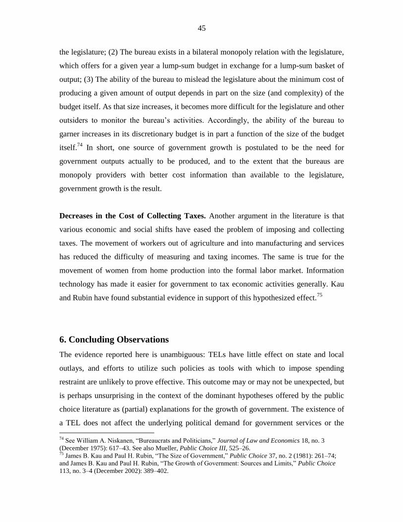
45

the legislature; (2) The bureau exists in a bilateral monopoly relation with the legislature,

which offers for a given year a lump-sum budget in exchange for a lump-sum basket of

output; (3) The ability of the bureau to mislead the legislature about the minimum cost of

producing a given amount of output depends in part on the size (and complexity) of the

budget itself. As that size increases, it becomes more difficult for the legislature and other

outsiders to monitor the bureau’s activities. Accordingly, the ability of the bureau to

garner increases in its discretionary budget is in part a function of the size of the budget

itself.74

In short, one source of government growth is postulated to be the need for

government outputs actually to be produced, and to the extent that the bureaus are

monopoly providers with better cost information than available to the legislature,

government growth is the result.

Decreases in the Cost of Collecting Taxes. Another argument in the literature is that

various economic and social shifts have eased the problem of imposing and collecting

taxes. The movement of workers out of agriculture and into manufacturing and services

has reduced the difficulty of measuring and taxing incomes. The same is true for the

movement of women from home production into the formal labor market. Information

technology has made it easier for government to tax economic activities generally. Kau

and Rubin have found substantial evidence in support of this hypothesized effect.75

6. Concluding Observations

The evidence reported here is unambiguous: TELs have little effect on state and local

outlays, and efforts to utilize such policies as tools with which to impose spending

restraint are unlikely to prove effective. This outcome may or may not be unexpected, but

is perhaps unsurprising in the context of the dominant hypotheses offered by the public

choice literature as (partial) explanations for the growth of government. The existence of

a TEL does not affect the underlying political demand for government services or the

74

See William A. Niskanen, “Bureaucrats and Politicians,” Journal of Law and Economics 18, no. 3

(December 1975): 617–43. See also Mueller, Public Choice III, 525–26. 75

James B. Kau and Paul H. Rubin, “The Size of Government,” Public Choice 37, no. 2 (1981): 261–74;

and James B. Kau and Paul H. Rubin, “The Growth of Government: Sources and Limits,” Public Choice

113, no. 3–4 (December 2002): 389–402.

46

relative prices, incomes, or taste variables that drive such demands. It is likely that tax

levels or rates or the distribution of the tax burden is determined separately (or in partial

isolation) from the implementation of a TEL.

Moreover, the effect of taxes on work effort, and even more so on the distribution

of “ability” or productivity, is very likely to be independent of the implementation of a

TEL. Accordingly, the effect of redistribution and the taxes needed to finance it on the

demands for increased government spending is unlikely to be changed by the existence of

a TEL. Nor can the presence of a TEL affect the relative political influence of

concentrated and unconcentrated interests (other things equal), and the expansion in the

number of interests attendant upon a growing economy is likely to strengthen pressures

for more spending. The presence of a TEL cannot improve the information about bureau

costs available to the legislature, and it cannot reverse the declining costs of tax

collection.

In short, a TEL is unlikely by itself to reverse the underlying conditions that yield

expanding government. In particular, the incentives of interest groups to circumvent and

neutralize the effects of TELs are unsurprising; that may be one central lesson from the

California and Washington experiences. Future efforts to restrain the growth in

government spending may find greater success if they are directed at increasing

competition among bureaus. One obvious way to achieve this is to strengthen the

institutions of federalism, thus forcing states and localities to compete with each other.

Another might be to allow bureaus to compete for budget dollars in the provision of

given services. An expanded effort to privatize the provision of government services in a

competitive market might serve to improve productivity and reduce costs. More

generally, it is likely to be the case that such mechanical tools as TELs will be unable to

substitute for the hard work of long-term public education and persuasion about the

central benefits of reduced government spending. At a fundamental level, in the long run

under democratic institutions, popular will is likely to impose sharp constraints on the

behavior of government; this means that attitudes must be changed through a process of

debate and enlightenment.

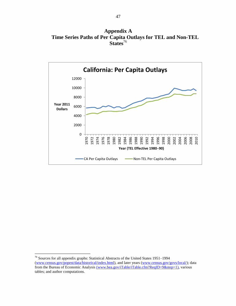
47

Appendix A

Time Series Paths of Per Capita Outlays for TEL and Non-TEL

States76

76

Sources for all appendix graphs: Statistical Abstracts of the United States 1951–1994

(www.census.gov/popest/data/historical/index.html), and later years (www.census.gov/govs/local/); data

from the Bureau of Economic Analysis (www.bea.gov/iTable/iTable.cfm?ReqID=9&step=1), various

tables; and author computations.

0

2000

4000

6000

8000

10000

12000

19

70

19

72

19

74

19

76

19

78

19

80

19

82

19

84

19

86

19

88

19

90

19

92

19

94

19

96

19

98

20

00

20

02

20

04

20

06

20

08

20

10

Year 2011 Dollars

Year (TEL Effective 1980–90)

California: Per Capita Outlays

CA Per Capita Outlays Non-TEL Per Capita Outlays

48

0

2000

4000

6000

8000

10000

12000

19

70

19

72

19

74

19

76

19

78

19

80

19

82

19

84

19

86

19

88

19

90

19

92

19

94

19

96

19

98

20

00

20

02

20

04

20

06

20

08

20

10

Year 2011 Dollars

Year (TEL Effective 1991–2010)

Connecticut: Per Capita Outlays

CT Per Capita Outlays Non-TEL Per Capita Outlays

0

2000

4000

6000

8000

10000

12000

19

70

19

72

19

74

19

76

19

78

19

80

19

82

19

84

19

86

19

88

19

90

19

92

19

94

19

96

19

98

20

00

20

02

20

04

20

06

20

08

20

10

Year 2011 Dollars

Year (TEL Effective 1979–2010)

Delaware: Per Capita Outlays

DE Per Capita Outlays Non-TEL Per Capita Outlays

49

0

2000

4000

6000

8000

10000

19

70

19

72

19

74

19

76

19

78

19

80

19

82

19

84

19

86

19

88

19

90

19

92

19

94

19

96

19

98

20

00

20

02

20

04

20

06

20

08

20

10

Year 2011 Dollars

Year (TEL Effective 1995–2010)

Florida: Per Capita Outlays

FL Per Capita Outlays Non-TEL Per Capita Outlays

0

2000

4000

6000

8000

10000

12000

19

70

19

72

19

74

19

76

19

78

19

80

19

82

19

84

19

86

19

88

19

90

19

92

19

94

19

96

19

98

20

00

20

02

20

04

20

06

20

08

20

10

Year 2011 Dollars

Year (TEL Effective 1979–2010)

Hawaii: Per Capita Outlays

HI Per Capita Outlays Non-TEL Per Capita Outlays

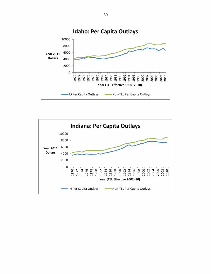
50

0

2000

4000

6000

8000

10000

19

70

19

72

19

74

19

76

19

78

19

80

19

82

19

84

19

86

19

88

19

90

19

92

19

94

19

96

19

98

20

00

20

02

20

04

20

06

20

08

20

10

Year 2011 Dollars

Year (TEL Effective 1980–2010)

Idaho: Per Capita Outlays

ID Per Capita Outlays Non-TEL Per Capita Outlays

0

2000

4000

6000

8000

10000

19

70

19

72

19

74

19

76

19

78

19

80

19

82

19

84

19

86

19

88

19

90

19

92

19

94

19

96

19

98

20

00

20

02

20

04

20

06

20

08

20

10

Year 2011 Dollars

Year (TEL Effective 2002–10)

Indiana: Per Capita Outlays

IN Per Capita Outlays Non-TEL Per Capita Outlays

51

0

2000

4000

6000

8000

10000

19

70

19

72

19

74

19

76

19

78

19

80

19

82

19

84

19

86

19

88

19

90

19

92

19

94

19

96

19

98

20

00

20

02

20

04

20

06

20

08

20

10

Year 2011 Dollars

Year (TEL Effective 1992–2010)

Iowa: Per Capita Outlays

IA Per Capita Outlays Non-TEL Per Capita Outlays

0

2000

4000

6000

8000

10000

12000

19

70

19

72

19

74

19

76

19

78

19

80

19

82

19

84

19

86

19

88

19

90

19

92

19

94

19

96

19

98

20

00

20

02

20

04

20

06

20

08

20

10

Year 2011 Dollars

Year (TEL Effective 1993–2010)

Louisiana: Per Capita Outlays

LA Per Capita Outlays Non-TEL Per Capita Outlays

52

0

2000

4000

6000

8000

10000

19

70

19

72

19

74

19

76

19

78

19

80

19

82

19

84

19

86

19

88

19

90

19

92

19

94

19

96

19

98

20

00

20

02

20

04

20

06

20

08

20

10

Year 2011 Dollars

Year (TEL Effective 2005–10)

Maine: Per Capita Outlays

ME Per Capita Outlays Non-TEL Per Capita Outlays

0

2000

4000

6000

8000

10000

12000

Year 2011 Dollars

Year (TEL Effective 1986–2010)

Massachusetts: Per Capita Outlays

MA Per Capita Outlays Non-TEL Per Capita Outlays

53

0

2000

4000

6000

8000

10000

19

70

19

72

19

74

19

76

19

78

19

80

19

82

19

84

19

86

19

88

19

90

19

92

19

94

19

96

19

98

20

00

20

02

20

04

20

06

20

08

20

10

Year 2011 Dollars

Year (TEL Effective 1979–2010)

Michigan: Per Capita Outlays

MI Per Capita Outlays Non-TEL Per Capita Outlays

0

2000

4000

6000

8000

10000

Year 2011 Dollars

Year (TEL Effective 1983–2010)

Mississippi: Per Capita Outlays

MS Per Capita Outlays Non-TEL Per Capita Outlays

54

0

2000

4000

6000

8000

10000

19

70

19

72

19

74

19

76

19

78

19

80

19

82

19

84

19

86

19

88

19

90

19

92

19

94

19

96

19

98

20

00

20

02

20

04

20

06

20

08

20

10

Year 2011 Dollars

Year (TEL Effective 1980–2010)

Missouri: Per Capita Outlays

MO Per Capita Outlays Non-TEL Per Capita Outlays

0

2000

4000

6000

8000

10000

19

70

19

72

19

74

19

76

19

78

19

80

19

82

19

84

19

86

19

88

19

90

19

92

19

94

19

96

19

98

20

00

20

02

20

04

20

06

20

08

20

10

Year 2011 Dollars

Year (TEL Effective 1981–2005)

Montana: Per Capita Outlays

MT Per Capita Outlays Non-TEL Per Capita Outlays

55

0

2000

4000

6000

8000

10000

Year 2011 Dollars

Year (TEL Effective 1980–2010)

Nevada: Per Capita Outlays

NV Per Capita Outlays Non-TEL Per Capita Outlays

0

2000

4000

6000

8000

10000

12000

19

70

19

72

19

74

19

76

19

78

19

80

19

82

19

84

19

86

19

88

19

90

19

92

19

94

19

96

19

98

20

00

20

02

20

04

20

06

20

08

20

10

Year 2011 Dollars

Year (TEL Effective 1990–2010)

New Jersey: Per Capita Outlays

NJ Per Capita Outlays Non-TEL Per Capita Outlays

56

0

2000

4000

6000

8000

10000

19

70

19

72

19

74

19

76

19

78

19

80

19

82

19

84

19

86

19

88

19

90

19

92

19

94

19

96

19

98

20

00

20

02

20

04

20

06

20

08

20

10

Year 2011 Dollars

Year (TEL Effective 1991–2010)

North Carolina: Per Capita Outlays

NC Per Capita Outlays Non-TEL Per Capita Outlays

0

2000

4000

6000

8000

10000

Year 2011 Dollars

Year (TEL Effective 2007–10)

Ohio: Per Capita Outlays

OH Per Capita Outlays Non-TEL Per Capita Outlays

57

0

2000

4000

6000

8000

10000

Year 2011 Dollars

Year (TEL Effective 1986–2010)

Oklahoma: Per Capita Outlays

OK Per Capita Outlays Non-TEL Per Capita Outlays

0

2000

4000

6000

8000

10000

12000

Year 2011 Dollars

Year (TEL Effective 2001–10)

Oregon: Per Capita Outlays

OR Per Capita Outlays Non-TEL Per Capita Outlays

58

0

2000

4000

6000

8000

10000

Year 2011 Dollars

Year (TEL Effective 1992–2010)

Rhode Island: Per Capita Outlays

RI Per Capita Outlays Non-TEL Per Capita Outlays

0

2000

4000

6000

8000

10000

Year 2011 Dollars

Year (TEL Effective 1978–2010)

Tennessee: Per Capita Outlays

TN Per Capita Outlays Non-TEL Per Capita Outlays

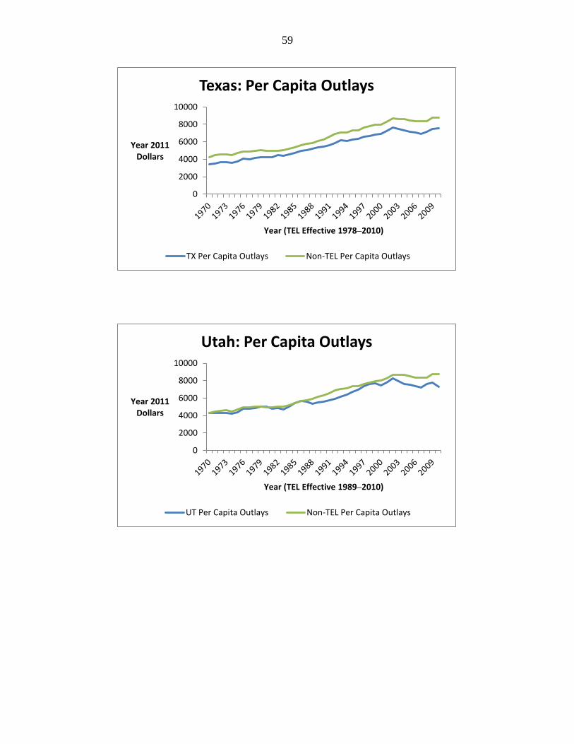
59

0

2000

4000

6000

8000

10000

Year 2011 Dollars

Year (TEL Effective 1978–2010)

Texas: Per Capita Outlays

TX Per Capita Outlays Non-TEL Per Capita Outlays

0

2000

4000

6000

8000

10000

Year 2011 Dollars

Year (TEL Effective 1989–2010)

Utah: Per Capita Outlays

UT Per Capita Outlays Non-TEL Per Capita Outlays

60

0

2000

4000

6000

8000

10000

Year 2011 Dollars

Year (TEL Effective 2001–10)

Wisconsin: Per Capita Outlays

WI Per Capita Outlays Non-TEL Per Capita Outlays

61

About the Author

Benjamin Zycher (benjamin.zycher@aei.org) is a visiting scholar at the American

Enterprise Institute.

Acknowledgments

Sincere thanks are due the National Research Initiative program at AEI for generous

financial support of this work, but the views expressed are the author’s alone and do not

purport to represent those of AEI or of any of its officers or sponsors. I am indebted as

well to William R. Allen, Wayne T. Brough, Richard J. Buddin, Laurence A. Dougharty,

Michael J. New, Henry Olsen, Mark J. Perry, and Bradley J. Wassink for comments and

suggestions. The author alone is responsible for any remaining errors.