Standard Costs and Operating Performance Measures · PDF fileUploaded By Qasim Mughal ...
84
Uploaded By Qasim Mughal http://world-best-free.blogspot.com/ Chapter 11 Standard Costs and Operating Performance Measures Solutions to Questions 11-1 A quantity standard indicates how much of an input should be used to make a unit of output. A price standard indicates how much the input should cost. 11-2 Ideal standards assume perfection and do not allow for any inefficiency. Ideal standards are rarely, if ever, attained. Practical standards can be attained by employees working at a reasonable, though efficient pace and allow for normal breaks and work interruptions. 11-3 Under management by exception, managers focus their attention on results that deviate from expectations. It is assumed that results that meet expectations do not require investigation. 11-4 Separating an overall variance into a price variance and a quantity variance provides more information. Moreover, price and quantity variances are usually the responsibilities of different managers. 11-5 The materials price variance is usually the responsibility of the purchasing manager. The materials quantity and labor efficiency variances are usually the responsibility of production managers and supervisors. 11-6 The materials price variance can be computed either when materials are purchased or when they are placed into production. It is usually better to compute the variance when materials are purchased because that is when the purchasing manager, who has responsibility for this variance, has completed his or her work. In addition, recognizing the price variance when materials are purchased allows the company to carry its raw materials in the inventory accounts at standard cost, which greatly simplifies bookkeeping. 11-7 This combination of variances may indicate that inferior quality materials were purchased at a discounted price, but the low- quality materials created production problems. 11-8 If standards are used to find who to blame for problems, they can breed resentment and undermine morale. Standards should not be used to find someone to blame for problems. 11-9 Several factors other than the contractual rate paid to workers can cause a labor rate variance. For example, skilled workers with high hourly rates of pay can be given duties that require little skill and that call for low hourly rates of pay, resulting in an unfavorable rate variance. Or unskilled or untrained workers can be assigned to tasks that should be filled by more skilled workers with higher rates of pay, resulting in a favorable rate variance. Unfavorable rate variances can also arise from overtime work at premium rates. 11-10 If poor quality materials create production problems, a result could be excessive labor time and therefore an unfavorable labor efficiency variance. Poor © The McGraw-Hill Companies, Inc., 2010 30 Managerial Accounting, 13th Edition
Transcript of Standard Costs and Operating Performance Measures · PDF fileUploaded By Qasim Mughal ...

Uploaded By Qasim Mughal
http://world-best-free.blogspot.com/
Chapter 11Standard Costs and Operating Performance Measures
Solutions to Questions
11-1 A quantity standard indicates how much of an input should be used to make a unit of output. A price standard indicates how much the input should cost.
11-2 Ideal standards assume perfection and do not allow for any inefficiency. Ideal standards are rarely, if ever, attained. Practical standards can be attained by employees working at a reasonable, though efficient pace and allow for normal breaks and work interruptions.
11-3 Under management by exception, managers focus their attention on results that deviate from expectations. It is assumed that results that meet expectations do not require investigation.
11-4 Separating an overall variance into a price variance and a quantity variance provides more information. Moreover, price and quantity variances are usually the responsibilities of different managers.
11-5 The materials price variance is usually the responsibility of the purchasing manager. The materials quantity and labor efficiency variances are usually the responsibility of production managers and supervisors.
11-6 The materials price variance can be computed either when materials are purchased or when they are placed into production. It is usually better to compute the variance when materials are purchased because that is when
the purchasing manager, who has responsibility for this variance, has completed his or her work. In addition, recognizing the price variance when materials are purchased allows the company to carry its raw materials in the inventory accounts at standard cost, which greatly simplifies bookkeeping.
11-7 This combination of variances may indicate that inferior quality materials were purchased at a discounted price, but the low-quality materials created production problems.
11-8 If standards are used to find who to blame for problems, they can breed resentment and undermine morale. Standards should not beused to find someone to blame for problems.
11-9 Several factors other than the contractual rate paid to workers can cause a labor rate variance. For example, skilled workerswith high hourly rates of pay can be given dutiesthat require little skill and that call for low hourly rates of pay, resulting in an unfavorable rate variance. Or unskilled or untrained workers can be assigned to tasks that should be filled by more skilled workers with higher rates of pay, resulting in a favorable rate variance. Unfavorable rate variances can also arise from overtime work at premium rates.
11-10 If poor quality materials create production problems, a result could be excessive labor time and therefore an unfavorable labor efficiency variance. Poor
© The McGraw-Hill Companies, Inc., 2010
30 Managerial Accounting, 13th Edition

quality materials would not ordinarily affect the labor rate variance.
11-11 If overhead is applied on the basis of direct labor-hours, then the variable overhead efficiency variance and the direct labor efficiencyvariance will always be favorable or unfavorable together. Both variances are computed by comparing the number of direct labor-hours actually worked to the standard hours allowed. That is, in each case the formula is:
Efficiency Variance = SR(AH – SH)
Only the “SR” part of the formula, the standard rate, differs between the two variances.
11-12 A statistical control chart is a graphical aid that helps identify variances that should be investigated. Upper and lower limits are set on the control chart. Any variances falling between those limits are considered to be normal. Any variances falling outside of those limits are considered abnormal and are investigated.
11-13 If labor is a fixed cost and standards are tight, then the only way to generate favorable labor efficiency variances is for every workstation to produce at capacity. However, theoutput of the entire system is limited by the
capacity of the bottleneck. If workstations beforethe bottleneck in the production process produceat capacity, the bottleneck will be unable to process all of the work in process. In general, if every workstation is attempting to produce at capacity, then work in process inventory will build up in front of the workstations with the leastcapacity.
11-14 The difference between delivery cycle time and throughput time is the waiting period between when an order is received and when production on the order is started. Throughput time is made up of process time, inspection time, move time, and queue time. These four elements can be classified into value-added time(process time) and non-value-added time (inspection time, move time, and queue time).
11-15 An MCE of less than 1 means that the production process includes non-value-added time. An MCE of 0.40, for example, means that 40% of throughput time consists of actual processing, and that the other 60% consists of moving, inspection, and other non-value-added activities.
© The McGraw-Hill Companies, Inc., 2010
31 Managerial Accounting, 13th Edition

Exercise 11-1 (20 minutes)
1. Cost per 15-gallon container................................... $115.00Less 2% cash discount........................................... 2.30 Net cost................................................................... 112.70Add shipping cost per container ($130 ÷ 100)........ 1.30 Total cost per 15-gallon container (a)...................... $114.00Number of quarts per container
(15 gallons × 4 quarts per gallon) (b)................... 60Standard cost per quart purchased (a) ÷ (b)........... $1.90
2. Content per bill of materials............................... 7.6 quartsAdd allowance for evaporation and spillage
(7.6 quarts ÷ 0.95 = 8.0 quarts; 8.0 quarts – 7.6 quarts = 0.4 quarts).............. 0.4 quarts
Total................................................................... 8.0 quartsAdd allowance for rejected units
(8.0 quarts ÷ 40 bottles).................................. 0.2 quartsStandard quantity per salable bottle of solvent. . 8.2 quarts
3.Item
StandardQuantity Standard Price
Standard Costper Bottle
Echol 8.2 quarts $1.90 per quart $15.58
© The McGraw-Hill Companies, Inc., 2010. All rights reserved.
Solutions Manual, Chapter 11 32

Exercise 11-2 (20 minutes)
1. Number of helmets............................................... 35,000Standard kilograms of plastic per helmet.............. × 0.6 Total standard kilograms allowed......................... 21,000Standard cost per kilogram................................... × RM8 Total standard cost............................................... RM168,000
Actual cost incurred (given).................................. RM171,000Total standard cost (above).................................. 168,000 Total material variance—unfavorable................... RM 3,000
2. Actual Quantityof Input, at Actual Price
Actual Quantity of Input, at Standard Price
Standard Quantity Allowed for Output, at
Standard Price(AQ × AP) (AQ × SP) (SQ × SP)
22,500 kilograms × 21,000 kilograms* ×RM8 per kilogram RM8 per kilogram
RM171,000 = RM180,000 = RM168,000 ↑ ↑ ↑
Price Variance, RM9,000 F
Quantity Variance, RM12,000 U
Total Variance, RM3,000 U
*35,000 helmets × 0.6 kilograms per helmet = 21,000 kilograms
Alternatively, the variances can be computed using the formulas:
Materials price variance = AQ (AP – SP)22,500 kilograms (RM7.60 per kilogram* – RM8.00 per kilogram)
= RM9,000 F
* RM171,000 ÷ 22,500 kilograms = RM7.60 per kilogram
Materials quantity variance = SP (AQ – SQ)RM8 per kilogram (22,500 kilograms – 21,000 kilograms)
= RM12,000 U
© The McGraw-Hill Companies, Inc., 2010. All rights reserved.
33 Managerial Accounting, 13th Edition

Exercise 11-3 (20 minutes)
1. Number of meals prepared..................... 4,000Standard direct labor-hours per meal..... × 0.25 Total direct labor-hours allowed.............. 1,000Standard direct labor cost per hour......... × $9.75Total standard direct labor cost............... $9,750
Actual cost incurred................................ $9,600Total standard direct labor cost (above). 9,750 Total direct labor variance....................... $ 150 Favorable
2. Actual Hours of Input, at the Actual Rate
Actual Hours of Input,at the Standard Rate
Standard Hours Allowed for Output, at
the Standard Rate(AH × AR) (AH × SR) (SH × SR)960 hours ×
$10.00 per hour960 hours ×
$9.75 per hour1,000 hours ×$9.75 per hour
= $9,600 = $9,360 = $9,750
↑ ↑ ↑Rate Variance,
$240 UEfficiency Variance,
$390 FTotal Variance,
$150 F
Alternatively, the variances can be computed using the formulas:
Labor rate variance = AH(AR – SR)= 960 hours ($10.00 per hour – $9.75 per hour)= $240 U
Labor efficiency variance = SR(AH – SH)= $9.75 per hour (960 hours – 1,000 hours)= $390 F
© The McGraw-Hill Companies, Inc., 2010. All rights reserved.
Solutions Manual, Chapter 11 34

Exercise 11-4 (20 minutes)
1. Number of items shipped................................... 120,000Standard direct labor-hours per item................. × 0.02 Total direct labor-hours allowed......................... 2,400Standard variable overhead cost per hour......... × $3.25Total standard variable overhead cost............... $ 7,800
Actual variable overhead cost incurred.............. $7,360Total standard variable overhead cost (above). 7,800 Total variable overhead variance....................... $ 440 Favorable
2. Actual Hours of Input, at the Actual Rate
Actual Hours of Input,at the Standard Rate
Standard Hours Allowed for Output, at
the Standard Rate(AH × AR) (AH × SR) (SH × SR)
2,300 hours × $3.20 per hour*
2,300 hours × $3.25 per hour
2,400 hours × $3.25 per hour
= $7,360 = $7,475 = $7,800
↑ ↑ ↑Variable Overhead
Rate Variance, $115 FVariable Overhead Efficiency Variance,
$325 FTotal Variance,
$440 F
*$7,360 ÷ 2,300 hours = $3.20 per hour
Alternatively, the variances can be computed using the formulas:
Variable overhead rate variance:AH(AR – SR) = 2,300 hours ($3.20 per hour – $3.25 per hour)
= $115 F
Variable overhead efficiency variance:SR(AH – SH) = $3.25 per hour (2,300 hours – 2,400 hours)
= $325 F
© The McGraw-Hill Companies, Inc., 2010. All rights reserved.
35 Managerial Accounting, 13th Edition

Exercise 11-5 (20 minutes)
1. Throughput time = Process time + Inspection time + Move time + Queue time
= 2.7 days + 0.3 days + 1.0 days + 5.0 days = 9.0 days
2. Only process time is value-added time; therefore the manufacturing cycle efficiency (MCE) is:
-Value added time 2.7 daysMCE = = = 0.30
Throughput time 9.0 days
3. If the MCE is 30%, then 30% of the throughput time was spent in value-added activities. Consequently, the other 70% of the throughput time was spent in non-value-added activities.
4. Delivery cycle time = Wait time + Throughput time = 14.0 days + 9.0 days = 23.0 days
5. If all queue time is eliminated, then the throughput time drops to only 4 days (2.7 + 0.3 + 1.0). The MCE becomes:
-Value added time 2.7 daysMCE = = = 0.675
Throughput time 4.0 days
Thus, the MCE increases to 67.5%. This exercise shows quite dramatically how lean production can improve the efficiency of operations and reduce throughput time.
© The McGraw-Hill Companies, Inc., 2010. All rights reserved.
Solutions Manual, Chapter 11 36

Exercise 11-6 (20 minutes)
1. The standard price of a kilogram of white chocolate is determined as follows:
Purchase price, finest grade white chocolate......................... £7.50Less purchase discount, 8% of the purchase price of £7.50. . (0.60)Shipping cost from the supplier in Belgium............................ 0.30Receiving and handling cost.................................................. 0.04 Standard price per kilogram of white chocolate...................... £7.24
2. The standard quantity, in kilograms, of white chocolate in a dozen truffles is computed as follows:
Material requirements............................... 0.70Allowance for waste.................................. 0.03Allowance for rejects................................. 0.02Standard quantity of white chocolate........ 0.75
3. The standard cost of the white chocolate in a dozen truffles is determined as follows:
Standard quantity of white chocolate (a)....... 0.75 kilogramStandard price of white chocolate (b)............ £7.24 per kilogramStandard cost of white chocolate (a) × (b).... £5.43
© The McGraw-Hill Companies, Inc., 2010. All rights reserved.
37 Managerial Accounting, 13th Edition

Exercise 11-7 (30 minutes)
1. a. Notice in the solution below that the materials price variance is computed on the entire amount of materials purchased, whereas the materials quantity variance is computed only on the amount of materials used in production.
Actual Quantity of Input, at Actual Price
Actual Quantity of Input, at Standard Price
Standard Quantity Allowed for Output, at
Standard Price(AQ × AP) (AQ × SP) (SQ × SP)
25,000 microns ×$0.48 per micron
25,000 microns ×$0.50 per micron
18,000 microns* ×$0.50 per micron
= $12,000 = $12,500 = $9,000
↑ ↑ ↑Price Variance,
$500 F20,000 microns × $0.50 per micron
= $10,000
↑Quantity Variance,
$1,000 U
*3,000 toys × 6 microns per toy = 18,000 microns
Alternatively, the variances can be computed using the formulas:
Materials price variance = AQ (AP – SP) 25,000 microns ($0.48 per micron – $0.50 per micron) = $500 F
Materials quantity variance = SP (AQ – SQ)$0.50 per micron (20,000 microns – 18,000 microns) = $1,000 U
© The McGraw-Hill Companies, Inc., 2010. All rights reserved.
Solutions Manual, Chapter 11 38

Exercise 11-7 (continued)
b. Direct labor variances:
Actual Hours of Input, at the Actual Rate
Actual Hours of Input,at the Standard Rate
Standard Hours Allowedfor Output, at the
Standard Rate(AH × AR) (AH × SR) (SH × SR)
4,000 hours ×$8.00 per hour
3,900 hours* ×$8.00 per hour
$36,000 = $32,000 = $31,200
↑ ↑ ↑Rate Variance,
$4,000 UEfficiency Variance,
$800 UTotal Variance,
$4,800 U
*3,000 toys × 1.3 hours per toy = 3,900 hours
Alternatively, the variances can be computed using the formulas:
Labor rate variance = AH (AR – SR) 4,000 hours ($9.00 per hour* – $8.00 per hour) = $4,000 U
*$36,000 ÷ 4,000 hours = $9.00 per hour
Labor efficiency variance = SR (AH – SH)$8.00 per hour (4,000 hours – 3,900 hours) = $800 U
© The McGraw-Hill Companies, Inc., 2010. All rights reserved.
39 Managerial Accounting, 13th Edition

Exercise 11-7 (continued)
2. A variance usually has many possible explanations. In particular, we should always keep in mind that the standards themselves may be incorrect. Some of the other possible explanations for the variances observed at Dawson Toys appear below:
Materials Price Variance Since this variance is favorable, the actual price paid per unit for the material was less than the standard price. This could occur for a variety of reasons including the purchase of a lower grade material at a discount, buying in an unusually large quantity to take advantage of quantity discounts, a change in the market price of the material, or particularly sharp bargaining by the purchasing department.
Materials Quantity Variance Since this variance is unfavorable, more materials were used to produce the actual output than were called for by the standard. This could also occur for a variety of reasons. Some of the possibilities include poorly trained or supervised workers, improperly adjusted machines, and defective materials.
Labor Rate Variance Since this variance is unfavorable, the actual average wage rate was higher than the standard wage rate. Some of the possible explanations include an increase in wages that has not been reflected in the standards, unanticipated overtime, and a shift toward morehighly paid workers.
Labor Efficiency Variance Since this variance is unfavorable, the actual number of labor hours was greater than the standard labor hours allowed for the actual output. As with the other variances, this variance could have been caused by any of a number of factors. Some of the possible explanations include poor supervision, poorly trained workers, low-quality materials requiring more labor time to process, and machine breakdowns. In addition, if the direct labor force is essentially fixed, an unfavorable labor efficiency variance could be caused by a reduction in output due to decreased demand for the company’s products.
It is worth noting that all of these variances could have been caused by the purchase of low quality materials at a cut-rate price.
© The McGraw-Hill Companies, Inc., 2010. All rights reserved.
Solutions Manual, Chapter 11 40

Exercise 11-8 (20 minutes)
1. Actual Quantity of Input, at Actual Price
Actual Quantity of Input, at
Standard Price
Standard QuantityAllowed for Output,at Standard Price
(AQ × AP) (AQ × SP) (SQ × SP)20,000 pounds ×$2.35 per pound
20,000 pounds ×$2.50 per pound
18,400 pounds* ×$2.50 per pound
= $47,000 = $50,000 = $46,000
↑ ↑ ↑Price Variance,
$3,000 FQuantity Variance,
$4,000 UTotal Variance,
$1,000 U
*4,000 units × 4.6 pounds per unit = 18,400 pounds
Alternatively, the variances can be computed using the formulas:
Materials price variance = AQ (AP – SP)20,000 pounds ($2.35 per pound – $2.50 per pound) = $3,000 F
Materials quantity variance = SP (AQ – SQ)$2.50 per pound (20,000 pounds – 18,400 pounds) = $4,000 U
© The McGraw-Hill Companies, Inc., 2010. All rights reserved.
41 Managerial Accounting, 13th Edition

Exercise 11-8 (continued)
2. Actual Hours of Input, at the Actual Rate
Actual Hours of Input,at the Standard Rate
Standard Hours Allowed for Output, at
the Standard Rate(AH × AR) (AH × SR) (SH × SR)
750 hours ×$12.00 per hour
800 hours* ×$12.00 per hour
$10,425 = $9,000 = $9,600
↑ ↑ ↑Rate Variance,
$1,425 UEfficiency Variance,
$600 FTotal Variance,
$825 U
*4,000 units × 0.2 hours per unit = 800 hours
Alternatively, the variances can be computed using the formulas:
Labor rate variance = AH (AR – SR)750 hours ($13.90 per hour* – $12.00 per hour) = $1,425 U
*10,425 ÷ 750 hours = $13.90 per hour
Labor efficiency variance = SR (AH – SH)$12.00 per hour (750 hours – 800 hours) = $600 F
© The McGraw-Hill Companies, Inc., 2010. All rights reserved.
Solutions Manual, Chapter 11 42

Exercise 11-9 (15 minutes)
Notice in the solution below that the materials price variance is computed for the entire amount of materials purchased, whereas the materials quantity variance is computed only for the amount of materials used in production.
Actual Quantity ofInput, at Actual Price
Actual Quantity of Input, at
Standard Price
Standard QuantityAllowed for Output,at Standard Price
(AQ × AP) (AQ × SP) (SQ × SP)20,000 pounds ×$2.35 per pound
20,000 pounds ×$2.50 per pound
13,800 pounds* ×$2.50 per pound
= $47,000 = $50,000 = $34,500
↑ ↑ ↑Price Variance,
$3,000 F14,750 pounds × $2.50 per pound = $36,875
↑Quantity Variance,
$2,375 U
*3,000 units × 4.6 pounds per unit = 13,800 pounds
Alternatively, the variances can be computed using the formulas:
Materials price variance = AQ (AP – SP)20,000 pounds ($2.35 per pound – $2.50 per pound) = $3,000 F
Materials quantity variance = SP (AQ – SQ)$2.50 per pound (14,750 pounds – 13,800 pounds) = $2,375 U
© The McGraw-Hill Companies, Inc., 2010. All rights reserved.
43 Managerial Accounting, 13th Edition

Exercise 11-10 (30 minutes)
1. Number of units manufactured................................ 20,000Standard labor time per unit
(18 minutes ÷ 60 minutes per hour)..................... × 0.3 Total standard hours of labor time allowed.............. 6,000Standard direct labor rate per hour......................... × $12 Total standard direct labor cost............................... $72,000
Actual direct labor cost............................................ $73,600Standard direct labor cost....................................... 72,000 Total variance—unfavorable.................................... $ 1,600
2. Actual Hours of Input, at the Actual Rate
Actual Hours of Input, atthe Standard Rate
Standard Hours Allowedfor Output, at the
Standard Rate(AH × AR) (AH × SR) (SH × SR)
5,750 hours ×$12.00 per hour
6,000 hours* ×$12.00 per hour
$73,600 = $69,000 = $72,000
↑ ↑ ↑Rate Variance,
$4,600 UEfficiency Variance,
$3,000 FTotal Variance,
$1,600 U
*20,000 units × 0.3 hours per unit = 6,000 hours
Alternatively, the variances can be computed using the formulas:
Labor rate variance = AH (AR – SR) 5,750 hours ($12.80 per hour* – $12.00 per hour) = $4,600 U
*$73,600 ÷ 5,750 hours = $12.80 per hour
Labor efficiency variance = SR (AH – SH) $12.00 per hour (5,750 hours – 6,000 hours) = $3,000 F
© The McGraw-Hill Companies, Inc., 2010. All rights reserved.
Solutions Manual, Chapter 11 44

Exercise 11-10 (continued)
3. Actual Hours of Input, at the Actual Rate
Actual Hours of Input,at the Standard Rate
Standard Hours Allowed for Output, at
the Standard Rate(AH × AR) (AH × SR) (SH × SR)
5,750 hours ×$4.00 per hour
6,000 hours ×$4.00 per hour
$21,850 = $23,000 = $24,000
↑ ↑ ↑Rate Variance,
$1,150 FEfficiency Variance,
$1,000 FTotal Variance,
$2,150 F
Alternatively, the variances can be computed using the formulas:
Variable overhead rate variance = AH (AR – SR)5,750 hours ($3.80 per hour* – $4.00 per hour) = $1,150 F
*$21,850 ÷ 5,750 hours = $3.80 per hour
Variable overhead efficiency variance = SR (AH – SH)$4.00 per hour (5,750 hours – 6,000 hours) = $1,000 F
© The McGraw-Hill Companies, Inc., 2010. All rights reserved.
45 Managerial Accounting, 13th Edition

Exercise 11-11 (20 minutes)
1. If the total variance is $93 unfavorable, and the rate variance is $87 favorable, then the efficiency variance must be $180 unfavorable, because the rate and efficiency variances taken together always equal the total variance. Knowing that the efficiency variance is $180 unfavorable, one approach to the solution would be:
Efficiency variance = SR (AH – SH) $9.00 per hour (AH – 125 hours*) = $180 U $9.00 per hour × AH – $1,125 = $180**$9.00 per hour × AH = $1,305 AH = $1,305 ÷ $9.00 per hour AH = 145 hours
*50 jobs × 2.5 hours per job = 125 hours**When used with the formula, unfavorable variances are positive and
favorable variances are negative.
2. Rate variance = AH (AR – SR) 145 hours (AR – $9.00 per hour) = $87 F145 hours × AR – $1,305 = –$87*145 hours × AR = $1,218 AR = $1,218 ÷ 145 hours AR = $8.40 per hour
*When used with the formula, unfavorable variances are positive and favorable variances are negative.
© The McGraw-Hill Companies, Inc., 2010. All rights reserved.
Solutions Manual, Chapter 11 46

Exercise 11-11 (continued)
An alternative approach would be to work from known to unknown data in the columnar model for variance analysis:
Actual Hours of Input, atthe Actual Rate
Actual Hours of Input,at the Standard Rate
Standard Hours Allowed for Output, at
the Standard Rate(AH × AR) (AH × SR) (SH × SR)
145 hours ×$8.40 per hour
145 hours ×$9.00 per hour*
125 hours§ ×$9.00 per hour*
= $1,218 = $1,305 = $1,125
↑ ↑ ↑Rate Variance,
$87 F*Efficiency Variance,
$180 UTotal Variance,
$93 U*§50 tune-ups* × 2.5 hours per tune-up* = 125 hours*Given
© The McGraw-Hill Companies, Inc., 2010. All rights reserved.
47 Managerial Accounting, 13th Edition

Problem 11-12 (45 minutes)
1. a. In the solution below, the materials price variance is computed on the entire amount of materials purchased whereas the materials quantity variance is computed only on the amount of materials used in production:
Actual Quantity ofInput, at
Actual Price
Actual Quantity of Input, at
Standard Price
Standard Quantity Allowed for Output, at
Standard Price(AQ × AP) (AQ × SP) (SQ × SP)
12,000 ounces ×$20.00 per ounce
9,375 ounces* ×$20.00 per ounce
$225,000 = $240,000 = $187,500
↑ ↑ ↑Price Variance,
$15,000 F9,500 ounces × $20.00 per ounce
= $190,000
↑Quantity Variance,
$2,500 U
*3,750 units × 2.5 ounces per unit = 9,375 ounces
Alternatively, the variances can be computed using the formulas:
Materials price variance = AQ (AP – SP)12,000 ounces ($18.75 per ounce* – $20.00 per ounce) = $15,000 F
*$225,000 ÷ 12,000 ounces = $18.75 per ounce
Materials quantity variance = SP (AQ – SQ) $20.00 per ounce (9,500 ounces – 9,375 ounces) = $2,500 U
b. Yes, the contract probably should be signed. The new price of $18.75 per ounce is substantially lower than the old price of $20.00 per ounce, resulting in a favorable price variance of $15,000 for the month. Moreover, the material from the new supplier appears to cause little or no problem in production as shown by the small materials quantity variance for the month.
© The McGraw-Hill Companies, Inc., 2010. All rights reserved.
Solutions Manual, Chapter 11 48

Problem 11-12 (continued)
2. a.Actual Hours of
Input, at the Actual Rate
Actual Hours of Input, at the
Standard Rate
Standard Hours Allowed for Output, at
the Standard Rate(AH × AR) (AH × SR) (SH × SR)
5,600 hours* ×$12.00 per hour
5,600 hours ×$12.50 per hour
5,250 hours** ×$12.50 per hour
= $67,200 = $70,000 = $65,625
↑ ↑ ↑Rate Variance,
$2,800 FEfficiency Variance,
$4,375 UTotal Variance,
$1,575 U
*35 technicians × 160 hours per technician = 5,600 hours**3,750 units × 1.4 hours per technician = 5,250 hrs
Alternatively, the variances can be computed using the formulas:
Labor rate variance = AH (AR – SR) 5,600 hours ($12.00 per hour – $12.50 per hour) = $2,800 F
Labor efficiency variance = SR (AH – SH) $12.50 per hour (5,600 hours – 5,250 hours) = $4,375 U
b. No, the new labor mix probably should not be continued. Although it decreases the average hourly labor cost from $12.50 to $12.00, thereby causing a $2,800 favorable labor rate variance, this savings ismore than offset by a large unfavorable labor efficiency variance for the month. Thus, the new labor mix increases overall labor costs.
© The McGraw-Hill Companies, Inc., 2010. All rights reserved.
49 Managerial Accounting, 13th Edition

Problem 11-12 (continued)
3. Actual Hours of Input, at the Actual Rate
Actual Hours of Input, at the
Standard Rate
Standard Hours Allowed for Output,
at the Standard Rate(AH × AR) (AH × SR) (SH × SR)
5,600 hours* ×$3.50 per hour
5,250 hours** ×$3.50 per hour
$18,200 = $19,600 = $18,375
↑ ↑ ↑Rate Variance,
$1,400 FEfficiency Variance,
$1,225 UTotal Variance,
$175 F
* Based on direct labor hours: 35 technicians × 160 hours per technician = 5,600 hours
** 3,750 units × 1.4 hours per unit = 5,250 hours
Alternatively, the variances can be computed using the formulas:
Variable overhead rate variance = AH (AR – SR)5,600 hours ($3.25 per hour* – $3.50 per hour) = $1,400 F
*$18,200 ÷ 5,600 hours = $3.25 per hour
Variable overhead efficiency variance = SR (AH – SH) $3.50 per hour (5,600 hours – 5,250 hours) = $1,225 U
Both the labor efficiency variance and the variable overhead efficiency variance are computed by comparing actual labor-hours to standard labor-hours. Thus, if the labor efficiency variance is unfavorable, then the variable overhead efficiency variance will be unfavorable as well.
© The McGraw-Hill Companies, Inc., 2010. All rights reserved.
Solutions Manual, Chapter 11 50

Problem 11-13 (30 minutes)
1. a., b., and c.Month
1 2 3 4Throughput time—days:
Process time (x)................................... 2.1 2.0 1.9 1.8Inspection time..................................... 0.6 0.7 0.7 0.6Move time............................................. 0.4 0.3 0.4 0.4Queue time........................................... 4.3 5.0 5.8 6.7Total throughput time (y)...................... 7.4 8.0 8.8 9.5
Manufacturing cycle efficiency (MCE):Process time (x) ÷
Throughput time (y)........................... 28.4% 25.0% 21.6% 18.9%
Delivery cycle time—days:Wait time from order to start of
production.......................................... 16.0 17.5 19.0 20.5Throughput time................................... 7.4 8.0 8.8 9.5 Total delivery cycle time....................... 23.4 25.5 27.8 30.0
2. All of the performance measures display unfavorable trends. Throughputtime per unit is increasing—largely because of an increase in queue time. Manufacturing cycle efficiency is declining and delivery cycle time is increasing. In addition, the percentage of on-time deliveries has dropped.
© The McGraw-Hill Companies, Inc., 2010. All rights reserved.
51 Managerial Accounting, 13th Edition
Problem 11-13 (continued)
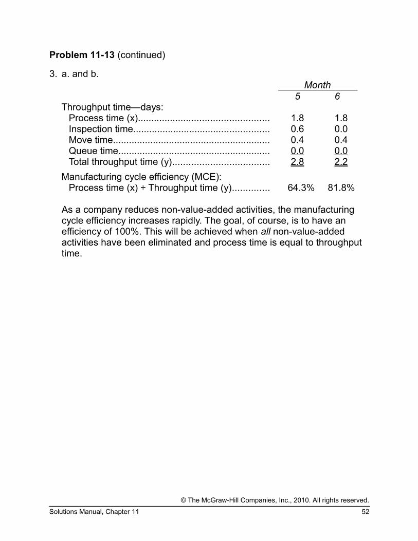
3. a. and b.Month
5 6Throughput time—days:
Process time (x)................................................. 1.8 1.8Inspection time................................................... 0.6 0.0Move time........................................................... 0.4 0.4Queue time......................................................... 0.0 0.0Total throughput time (y).................................... 2.8 2.2
Manufacturing cycle efficiency (MCE):Process time (x) ÷ Throughput time (y).............. 64.3% 81.8%
As a company reduces non-value-added activities, the manufacturing cycle efficiency increases rapidly. The goal, of course, is to have an efficiency of 100%. This will be achieved when all non-value-added activities have been eliminated and process time is equal to throughput time.
© The McGraw-Hill Companies, Inc., 2010. All rights reserved.
Solutions Manual, Chapter 11 52

Problem 11-14 (45 minutes)
1. a.
Actual Quantity ofInput, at Actual Price
Actual Quantity of Input, at
Standard Price
Standard QuantityAllowed for Output,at Standard Price
(AQ × AP) (AQ × SP) (SQ × SP)60,000 pounds ×$1.95 per pound
60,000 pounds ×$2.00 per pound
45,000 pounds* ×$2.00 per pound
= $117,000 = $120,000 = $90,000
↑ ↑ ↑Price Variance,
$3,000 F49,200 pounds × $2.00 per pound = $98,400
↑Quantity Variance,
$8,400 U
*15,000 pools × 3.0 pounds per pool = 45,000 pounds
Alternatively, the variances can be computed using the formulas:
Materials price variance = AQ (AP – SP) 60,000 pounds ($1.95 per pound – $2.00 per pound) = $3,000 F
Materials quantity variance = SP (AQ – SQ) $2.00 per pound (49,200 pounds – 45,000 pounds) = $8,400 U
© The McGraw-Hill Companies, Inc., 2010. All rights reserved.
53 Managerial Accounting, 13th Edition

Problem 11-14 (continued)
b.Actual Hours of
Input, at the Actual Rate
Actual Hours of Input,at the Standard Rate
Standard Hours Allowed for Output, at
the Standard Rate(AH × AR) (AH × SR) (SH × SR)
11,800 hours ×$7.00 per hour
11,800 hours ×$6.00 per hour
12,000 hours* ×$6.00 per hour
= $82,600 = $70,800 = $72,000
↑ ↑ ↑Rate Variance,
$11,800 UEfficiency Variance,
$1,200 FTotal Variance,
$10,600 U
*15,000 pools × 0.8 hours per pool = 12,000 hours
Alternatively, the variances can be computed using the formulas:
Labor rate variance = AH (AR – SR) 11,800 hours ($7.00 per hour – $6.00 per hour) = $11,800 U
Labor efficiency variance = SR (AH – SH) $6.00 per hour (11,800 hours – 12,000 hours) = $1,200 F
© The McGraw-Hill Companies, Inc., 2010. All rights reserved.
Solutions Manual, Chapter 11 54

Problem 11-14 (continued)
c.Actual Hours of
Input, at the Actual Rate
Actual Hours of Input, at the
Standard Rate
Standard Hours Allowed for Output, at
the Standard Rate(AH × AR) (AH × SR) (SH × SR)
5,900 hours ×$3.00 per hour
6,000 hours* ×$3.00 per hour
$18,290 = $17,700 = $18,000
↑ ↑ ↑Rate Variance,
$590 UEfficiency Variance,
$300 FTotal Variance,
$290 U
*15,000 pools × 0.4 hours per pool = 6,000 hours
Alternatively, the variances can be computed using the formulas:
Variable overhead rate variance = AH (AR – SR)5,900 hours ($3.10 per hour* – $3.00 per hour) = $590 U
*$18,290 ÷ 5,900 hours = $3.10 per hour
Variable overhead efficiency variance = SR (AH – SH) $3.00 per hour (5,900 hours – 6,000 hours) = $300 F
© The McGraw-Hill Companies, Inc., 2010. All rights reserved.
55 Managerial Accounting, 13th Edition

Problem 11-14 (continued)
2. Summary of variances:
Material price variance............................ $ 3,000 FMaterial quantity variance....................... 8,400 ULabor rate variance................................. 11,800 ULabor efficiency variance........................ 1,200 FVariable overhead rate variance............. 590 UVariable overhead efficiency variance.... 300 FNet variance........................................... $16,290 U
The net unfavorable variance of $16,290 for the month caused the plant’s variable cost of goods sold to increase from the budgeted level of$180,000 to $196,290:
Budgeted cost of goods sold at $12 per pool.......... $180,000Add the net unfavorable variance, as above........... 16,290 Actual cost of goods sold........................................ $196,290
This $16,290 net unfavorable variance also accounts for the difference between the budgeted net operating income and the actual net operating income for the month.
Budgeted net operating income............................... $36,000Deduct the net unfavorable variance added to cost
of goods sold for the month.................................. 16,290 Net operating income.............................................. $ 19 ,710
3. The two most significant variances are the materials quantity variance and the labor rate variance. Possible causes of the variances include:
Materials quantity variance: Outdated standards, unskilled workers,poorly adjusted machines, carelessness, poorly trained workers, inferior quality materials.
Labor rate variance: Outdated standards, change in pay scale, overtime pay.
© The McGraw-Hill Companies, Inc., 2010. All rights reserved.
Solutions Manual, Chapter 11 56

Problem 11-15 (45 minutes)
1. The standard quantity of plates allowed for tests performed during the month would be:
Blood tests..................................... 1,800Smears........................................... 2,400Total................................................ 4,200Plates per test................................ × 2 Standard quantity allowed.............. 8,400
The variance analysis for plates would be:
Actual Quantity ofInput, at Actual Price
Actual Quantity of Input, at
Standard Price
Standard QuantityAllowed for Output,at Standard Price
(AQ × AP) (AQ × SP) (SQ × SP)12,000 plates ×$2.50 per plate
8,400 plates ×$2.50 per plate
$28,200 = $30,000 = $21,000
↑ ↑ ↑Price Variance,
$1,800 F10,500 plates × $2.50 per plate = $26,250
↑Quantity Variance,
$5,250 U
Alternatively, the variances can be computed using the formulas:
Materials price variance = AQ (AP – SP)12,000 plates ($2.35 per plate* – $2.50 per plate) = $1,800 F
*$28,200 ÷ 12,000 plates = $2.35 per plate.
Materials quantity variance = SP (AQ – SQ) $2.50 per plate (10,500 plates – 8,400 plates) = $5,250 U
© The McGraw-Hill Companies, Inc., 2010. All rights reserved.
57 Managerial Accounting, 13th Edition

Problem 11-15 (continued)
Note that all of the price variance is due to the hospital’s 6% quantity discount. Also note that the $5,250 quantity variance for the month is equal to 25% of the standard cost allowed for plates.
2. a. The standard hours allowed for tests performed during the month would be:
Blood tests: 0.3 hour per test × 1,800 tests............. 540 hoursSmears: 0.15 hour per test × 2,400 tests................ 360 hoursTotal standard hours allowed................................... 900 hours
The variance analysis would be:
Actual Hours of Input, at the Actual Rate
Actual Hours of Input, atthe Standard Rate
Standard Hours Allowed for Output, at
the Standard Rate(AH × AR) (AH × SR) (SH × SR)
1,150 hours ×$14.00 per hour
900 hours ×$14.00 per hour
$13,800 = $16,100 = $12,600
↑ ↑ ↑Rate Variance,
$2,300 FEfficiency Variance,
$3,500 UTotal Variance,
$1,200 U
Alternatively, the variances can be computed using the formulas:
Labor rate variance = AH (AR – SR) 1,150 hours ($12.00 per hour* – $14.00 per hour) = $2,300 F
*$13,800 ÷ 1,150 hours = $12.00 per hour
Labor efficiency variance = SR (AH – SH) $14.00 per hour (1,150 hours – 900 hours) = $3,500 U
© The McGraw-Hill Companies, Inc., 2010. All rights reserved.
Solutions Manual, Chapter 11 58

Problem 11-15 (continued)
b. The policy probably should not be continued. Although the hospital is saving $2 per hour by employing more assistants than senior technicians, this savings is more than offset by other factors. Too much time is being taken in performing lab tests, as indicated by the large unfavorable labor efficiency variance. And, it seems likely that most (or all) of the hospital’s unfavorable quantity variance for plates is traceable to inadequate supervision of assistants in the lab.
3. The variable overhead variances follow:
Actual Hours of Input, at the Actual Rate
Actual Hours of Input,at the Standard Rate
Standard Hours Allowed for Output,
at the Standard Rate(AH × AR) (AH × SR) (SH × SR)
1,150 hours ×$6.00 per hour
900 hours ×$6.00 per hour
$7,820 = $6,900 = $5,400
↑ ↑ ↑Rate Variance,
$920 UEfficiency Variance,
$1,500 UTotal Variance,
$2,420 U
Alternatively, the variances can be computed using the formulas:
Variable overhead rate variance = AH (AR – SR) 1,150 hours ($6.80 per hour* – $6.00 per hour) = $920 U
*$7,820 ÷ 1,150 hours = $6.80 per hour
Variable overhead efficiency variance = SR (AH – SH)$6.00 per hour (1,150 hours – 900 hours) = $1,500 U
Yes, the two variances are closely related. Both are computed by comparing actual labor time to the standard hours allowed for the output of the period. Thus, if the labor efficiency variance is favorable (or unfavorable), then the variable overhead efficiency variance will also be favorable (or unfavorable).
© The McGraw-Hill Companies, Inc., 2010. All rights reserved.
59 Managerial Accounting, 13th Edition

Problem 11-16 (30 minutes)
1. Salex quantity standard:Required per 10-liter batch (9.6 liters ÷ 0.8)........... 12.0 litersLoss from rejected batches (1/5 × 12 liters)........... 2.4 litersTotal quantity per good batch................................. 14.4 liters
Nyclyn quantity standard:Required per 10-liter batch (12 kilograms ÷ 0.8).... 15.0 kilogramsLoss from rejected batches (1/5 × 15 kilograms)... 3.0 kilogramsTotal quantity per good batch................................. 18.0 kilograms
Protet quantity standard:Required per 10-liter batch.................................... 5.0 kilogramsLoss from rejected batches (1/5 × 5 kilograms)..... 1.0 kilogramsTotal quantity per good batch................................. 6.0 kilograms
2. Total minutes per 8-hour day.................................... 480 minutesLess rest breaks and cleanup................................... 60 minutesProductive time each day......................................... 420 minutes
Productive time each day 420 minutes per day =
Time required per batch 35 minutes per batch
= 12 batches per day
Time required per batch............................................ 35 minutesRest breaks and clean up time
(60 minutes ÷ 12 batches)..................................... 5 minutesTotal.......................................................................... 40 minutesLoss from rejected batches (1/5 × 40 minutes)........ 8 minutesTotal time per good batch......................................... 48 minutes
© The McGraw-Hill Companies, Inc., 2010. All rights reserved.
Solutions Manual, Chapter 11 60

Problem 11-16 (continued)
3. Standard cost card:Standard
Quantity orTime
Standard Price or Rate
StandardCost
Salex..................... 14.4 liters $1.50 per liter $21.60Nyclyn................... 18.0 kilograms $2.80 per kilogram 50.40Protet.................... 6.0 kilograms $3.00 per kilogram 18.00Labor time............. 48
or 0.8minutes, hour $9.00 per hour 7.20
Total standard costper acceptable batch.................. $97.20
© The McGraw-Hill Companies, Inc., 2010. All rights reserved.
61 Managerial Accounting, 13th Edition

Problem 11-17 (30 minutes)
1. a., b., and c.Month
1 2 3 4Throughput time in days:
Process time.................................... 2.1 2.0 1.9 1.8 Inspection time................................. 0.8 0.7 0.7 0.7 Move time........................................ 0.3 0.4 0.4 0.5 Queue time during production.......... 2.8 4.4 6.0 7.0 Total throughput time....................... 6.0 7.5 9.0 10.0
Manufacturing cycle efficiency (MCE):Process time ÷ Throughput time...... 35.0% 26.7% 21.1% 18.0%
Delivery cycle time in days:Wait time to start of production........ 9.0 11.5 12.0 14.0 Throughput time............................... 6.0 7.5 9.0 10.0 Total delivery cycle time................... 15.0 19.0 21.0 24.0
2. a. Areas where the company is improving:
Quality control. The number of defects has decreased by over 50% in the last four months. Moreover, both warranty claims and customer complaints are down sharply. In short, overall quality appears to have significantly improved.
Material control. The purchase order lead time is only half of what it was four months ago, which indicates that purchases are arriving in less time. This trend may be a result of the company’s move toward JIT purchasing.
Delivery performance. The process time has decreased from 2.1 daysto 1.8 days over the last four months.
© The McGraw-Hill Companies, Inc., 2010. All rights reserved.
Solutions Manual, Chapter 11 62

Problem 11-17 (continued)
b. Areas of deterioration:
Material control. Scrap as a percentage of total cost has tripled over the last four months.
Machine performance. Machine downtime has doubled over the last four months. This may be a result of the greater setup time, or it may just reflect efforts to get the new equipment operating properly. Also note that use of the machines as a percentage of availability is declining rapidly.
Delivery performance. All delivery performance measures are moving in the wrong direction. Throughput time and delivery cycle time are both increasing, and the manufacturing cycle efficiency is decreasing.
3. a. and b.Month
5 6Throughput time in days:
Process time............................................ 1.8 1.8 Inspection time......................................... 0.7 0.0 Move time................................................. 0.5 0.5 Queue time during production.................. 0.0 0.0 Total throughput time................................ 3.0 2.3
Manufacturing cycle efficiency (MCE):Process time ÷ Throughput time.............. 60.0% 78.3%
As non-value-added activities are eliminated, the manufacturing cycle efficiency improves. The goal, of course, is to have an efficiency of 100%. This is achieved when all non-value-added activities have been eliminated and process time equals throughput time.
© The McGraw-Hill Companies, Inc., 2010. All rights reserved.
63 Managerial Accounting, 13th Edition

Problem 11-18 (45 minutes)
This problem is more difficult than it looks. Allow ample time for discussion.
1.Actual Quantity of
Input, at Actual Price
Actual Quantity of Input, at
Standard Price
Standard QuantityAllowed for Output,at Standard Price
(AQ × AP) (AQ × SP) (SQ × SP)12,000 yards ×$4.00 per yard*
11,200 yards** ×$4.00 per yard*
$45,600 = $48,000 = $44,800
↑ ↑ ↑Price Variance,
$2,400 FQuantity Variance,
$3,200 UTotal Variance,
$800 U
* $22.40 ÷ 5.6 yards = $4.00 per yard** 2,000 sets × 5.6 yards per set = 11,200 yards
Alternatively, the variances can be computed using the formulas:
Materials price variance = AQ (AP – SP) 12,000 yards ($3.80 per yard* – $4.00 per yard) = $2,400 F
*$45,600 ÷ 12,000 yards = $3.80 per yard
Materials quantity variance = SP (AQ – SQ) $4.00 per yard (12,000 yards – 11,200 yards) = $3,200 U
© The McGraw-Hill Companies, Inc., 2010. All rights reserved.
Solutions Manual, Chapter 11 64

Problem 11-18 (continued)
2. Many students will miss parts 2 and 3 because they will try to use product costs as if they were hourly costs. Pay particular attention to the computation of the standard direct labor time per unit and the standard direct labor rate per hour.
Actual Hours of Input, at the Actual Rate
Actual Hours of Input, at the
Standard Rate
Standard Hours Allowed for Output,
at the Standard Rate(AH × AR) (AH × SR) (SH × SR)
2,800 hours ×$6.00 per hour*
3,000 hours** ×$6.00 per hour*
$18,200 = $16,800 = $18,000
↑ ↑ ↑Rate Variance,
$1,400 UEfficiency Variance,
$1,200 FTotal Variance,
$200 U
* 2,850 standard hours ÷ 1,900 sets = 1.5 standard hours per set, $9.00 standard cost per set ÷ 1.5 standard hours per set = $6.00 standard rate per hour.
** 2,000 sets × 1.5 standard hours per set = 3,000 standard hours.
Alternatively, the variances can be computed using the formulas:
Labor rate variance = AH (AR – SR) 2,800 hours ($6.50 per hour* – $6.00 per hour) = $1,400 U
*$18,200 ÷ 2,800 hours = $6.50 per hour
Labor efficiency variance = SR (AH – SH)$6.00 per hour (2,800 hours – 3,000 hours) = $1,200 F
© The McGraw-Hill Companies, Inc., 2010. All rights reserved.
65 Managerial Accounting, 13th Edition

Problem 11-18 (continued)
3. Actual Hours of Input, at the Actual Rate
Actual Hours of Input, at the
Standard Rate
Standard Hours Allowed for Output,
at the Standard Rate(AH × AR) (AH × SR) (SH × SR)
2,800 hours ×$2.40 per hour*
3,000 hours ×$2.40 per hour*
$7,000 = $6,720 = $7,200
↑ ↑ ↑Rate Variance,
$280 UEfficiency Variance,
$480 FTotal Variance,
$200 F
*$3.60 standard cost per set ÷ 1.5 standard hours per set = $2.40 standard rate per hour
Alternatively, the variances can be computed using the formulas:
Variable overhead rate variance = AH (AR – SR)2,800 hours ($2.50 per hour* – $2.40 per hour) = $280 U
*$7,000 ÷ 2,800 hours = $2.50 per hour
Variable overhead efficiency variance = SR (AH – SH)$2.40 per hour (2,800 hours – 3,000 hours) = $480 F
© The McGraw-Hill Companies, Inc., 2010. All rights reserved.
Solutions Manual, Chapter 11 66
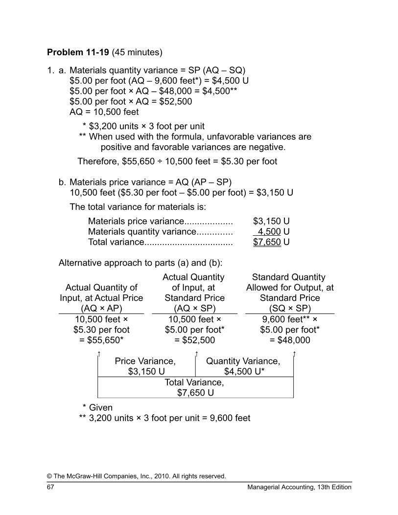
Problem 11-19 (45 minutes)
1. a. Materials quantity variance = SP (AQ – SQ)$5.00 per foot (AQ – 9,600 feet*) = $4,500 U$5.00 per foot × AQ – $48,000 = $4,500**$5.00 per foot × AQ = $52,500AQ = 10,500 feet
* $3,200 units × 3 foot per unit** When used with the formula, unfavorable variances are
positive and favorable variances are negative.
Therefore, $55,650 ÷ 10,500 feet = $5.30 per foot
b. Materials price variance = AQ (AP – SP)10,500 feet ($5.30 per foot – $5.00 per foot) = $3,150 U
The total variance for materials is:
Materials price variance................... $3,150 UMaterials quantity variance.............. 4,500 UTotal variance................................... $7,650 U
Alternative approach to parts (a) and (b):
Actual Quantity ofInput, at Actual Price
Actual Quantity of Input, at
Standard Price
Standard Quantity Allowed for Output, at
Standard Price(AQ × AP) (AQ × SP) (SQ × SP)
10,500 feet ×$5.30 per foot
10,500 feet ×$5.00 per foot*
9,600 feet** ×$5.00 per foot*
= $55,650* = $52,500 = $48,000
↑ ↑ ↑Price Variance,
$3,150 UQuantity Variance,
$4,500 U*Total Variance,
$7,650 U
* Given** 3,200 units × 3 foot per unit = 9,600 feet
© The McGraw-Hill Companies, Inc., 2010. All rights reserved.
67 Managerial Accounting, 13th Edition

Problem 11-19 (continued)
2. a. Labor rate variance = AH (AR – SR)4,900 hours ($7.50 per hour* – SR) = $2,450 F**$36,750 – 4,900 hours × SR = –$2,450***4,900 hours × SR = $39,200SR = $8.00
* $36,750 ÷ 4,900 hours** $1,650 F + $800 U.
*** When used with the formula, unfavorable variances are positive and favorable variances are negative.
b. Labor efficiency variance = SR (AH – SH) $8 per hour (4,900 hours – SH) = $800 U$39,200 – $8 per hour × SH = $800*$8 per hour × SH = $38,400SH = 4,800 hours
* When used with the formula, unfavorable variances are positiveand favorable variances are negative.
Alternative approach to parts (a) and (b):
Actual Hours of Input, at the Actual Rate
Actual Hours of Input, atthe Standard Rate
Standard Hours Allowed for Output, at the Standard Rate
(AH × AR) (AH × SR) (SH × SR)4,900 hours* ×$8.00 per hour
4,800 hours ×$8.00 per hour
$36,750* = $39,200 = $38,400
↑ ↑ ↑Rate Variance,
$2,450 FEfficiency Variance,
$800 U*Total Variance,
$1,650 F*
*Given.
c. The standard hours allowed per unit of product are:4,800 hours ÷ 3,200 units = 1.5 hours per unit
© The McGraw-Hill Companies, Inc., 2010. All rights reserved.
Solutions Manual, Chapter 11 68

Problem 11-21 (45 minutes)
1. Standard cost for a ten-gallon batch of raspberry sherbet.
Direct material:Raspberries (7.5 quarts1 × $0.80 per quart)................ $6.00Other ingredients (10 gallons × $0.45 per gallon)....... 4.50 $10.50
Direct labor:Sorting (18 minutes2 ÷ 60 minutes per hour) × $9.00
per hour.................................................................... 2.70Blending (12 minutes ÷ 60 minutes per hour) × $9.00
per hour.................................................................... 1.80 4.50Packing (40 quarts3 × $0.38 per quart)....................... 15.20
Standard cost per ten-gallon batch................................ $30.2016 quarts × (5 ÷ 4) = 7.5 quarts required to obtain 6 acceptable quarts.23 minutes per quart × 6 quarts.34 quarts per gallon × 10 gallons = 40 quarts.
2. a. In general, the purchasing manager is held responsible for unfavorable material price variances. Causes of these variances include the following:
• Incorrect standards.
• Failure to correctly forecast price increases.
• Purchasing in nonstandard or uneconomical lots.
• Failure to take available purchase discounts.
• Failure to control transportation costs.
• Purchasing from suppliers other than those offering the most favorable terms.
However, failure to meet price standards may be caused by an unexpected increase in orders or changes in production schedules. Inthis case, the responsibility for unfavorable material price variances should rest with the sales manager or the manager of production planning. Variances may also be caused by external events that are uncontrollable, e.g., a strike at a supplier’s plant.
© The McGraw-Hill Companies, Inc., 2010. All rights reserved.
69 Managerial Accounting, 13th Edition
Problem 11-21 (continued)
b. In general, the production manager or foreman is held responsible for unfavorable labor efficiency variances. Causes of these variances include the following:
• Incorrect standards.
• Poorly trained labor.
• Substandard or inefficient equipment.
• Inadequate supervision.
• Machine breakdowns from poor maintenance.
• Poorly motivated employees.
• Fixed labor force with demand less than capacity.
Failure to meet labor efficiency standards may also be caused by the use of inferior materials or poor production planning. In these cases, responsibility should rest with the purchasing manager or the manager of production planning. Variances may also be caused by external events that are uncontrollable, e.g., low unemployment leading to the inability to hire and retain skilled workers.
(Unofficial CMA Solution, adapted)
Uploaded By Qasim Mughal
http://world-best-free.blogspot.com/
© The McGraw-Hill Companies, Inc., 2010. All rights reserved.
Solutions Manual, Chapter 11 70

Case 11-22 (30 minutes)
This case may be difficult for some students to grasp because it requires looking at standard costs from an entirely different perspective. In this case,standard costs have been inappropriately used as a means to manipulate reported earnings rather than as a way to control costs.
1. Lansing has evidently set very loose standards in which the standard prices and standard quantities are far too high. This guarantees that favorable variances will ordinarily result from operations. If the standard costs are set artificially high, the standard cost of goods sold will be artificially high and thus the division’s net operating income will be depressed until the favorable variances are recognized. If Lansing savesthe favorable variances, he can release just enough in the second and third quarters to show some improvement and then he can release all of the rest in the last quarter, creating the annual “Christmas present.”
2. Lansing should not be permitted to continue this practice for several reasons. First, it distorts the quarterly earnings for both the division and the company. The distortions of the division’s quarterly earnings are troubling because the manipulations may mask real signs of trouble. Thedistortions of the company’s quarterly earnings are troubling because they may mislead external users of the financial statements. Second, Lansing should not be rewarded for manipulating earnings. This sets a moral tone in the company that is likely to lead to even deeper trouble. Indeed, the permissive attitude of top management toward the manipulation of earnings may indicate the existence of other, even more serious, ethical problems in the company. Third, a clear message shouldbe sent to division managers like Lansing that their job is to manage their operations, not their earnings. If they keep on top of operations andmanage well, the earnings should take care of themselves.
© The McGraw-Hill Companies, Inc., 2010. All rights reserved.
71 Managerial Accounting, 13th Edition

Case 11-22 (continued)
3. Stacy Cummins does not have any easy alternatives available. She has already taken the problem to the President, who was not interested. If she goes around the President to the Board of Directors, she will be putting herself in a politically difficult position with little likelihood that it will do much good if, in fact, the Board of Directors already knows what is going on.
On the other hand, if she simply goes along, she will be violating the Credibility standard of ethical conduct for management accountants. TheHome Security Division’s manipulation of quarterly earnings does distort the entire company’s quarterly reports. And the Credibility standard clearly stipulates that management accountants have a responsibility to “disclose all relevant information that could reasonably be expected to influence an intended user’s understanding of the reports, analyses, or recommendations.” Apart from the ethical issue, there is also a very practical consideration. If Merced Home Products becomes embroiled incontroversy concerning questionable accounting practices, Stacy Cummins will be viewed as a responsible party by outsiders and her career is likely to suffer dramatically and she may even face legal problems.
We would suggest that Ms. Cummins quietly bring the manipulation of earnings to the attention of the audit committee of the Board of Directors, carefully laying out in a non-confrontational manner the problems created by Lansing’s practice of manipulating earnings. If the President and the Board of Directors are still not interested in dealing with the problem, she may reasonably conclude that the best alternative is to start looking for another job.
© The McGraw-Hill Companies, Inc., 2010. All rights reserved.
Solutions Manual, Chapter 11 72
Case 11-23 (60 minutes)
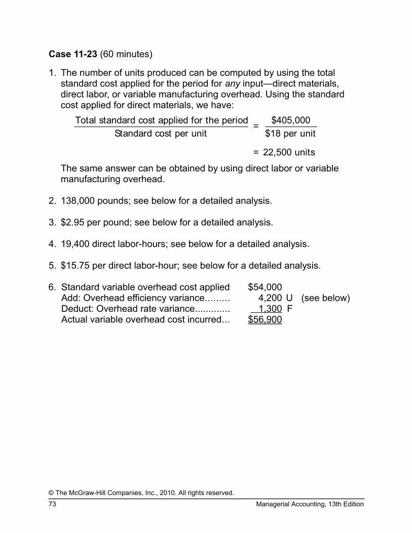
1. The number of units produced can be computed by using the total standard cost applied for the period for any input—direct materials, direct labor, or variable manufacturing overhead. Using the standard cost applied for direct materials, we have:
Total standard cost applied for the period $405,000 =
Standard cost per unit $18 per unit
= 22,500 units
The same answer can be obtained by using direct labor or variable manufacturing overhead.
2. 138,000 pounds; see below for a detailed analysis.
3. $2.95 per pound; see below for a detailed analysis.
4. 19,400 direct labor-hours; see below for a detailed analysis.
5. $15.75 per direct labor-hour; see below for a detailed analysis.
6. Standard variable overhead cost applied $54,000Add: Overhead efficiency variance......... 4,200 U (see below)Deduct: Overhead rate variance............. 1,300 FActual variable overhead cost incurred... $56,900
© The McGraw-Hill Companies, Inc., 2010. All rights reserved.
73 Managerial Accounting, 13th Edition

Case 11-23 (continued)
Direct materials analysis:
Actual Quantity of Inputs, at Actual
Price
Actual Quantity of Inputs, at
Standard Price
Standard QuantityAllowed for Output,at Standard Price
(AQ × AP) (AQ × SP) (SQ × SP)138,000 pounds
× $2.95 per pound***138,000 pounds**
× $3 per pound135,000 pounds* × $3 per pound
= $407,100 = $414,000 = $405,000
Price Variance, $6,900 F
Quantity Variance, $9,000 U
Total Variance, $2,100 U
* 22,500 units × 6 pounds per unit = 135,000 pounds** $414,000 ÷ $3 per pound = 138,000 pounds
*** $407,100 ÷ 138,000 pounds = $2.95 per pound
Direct labor analysis:
Actual Hours of Input,at the Actual Rate
Actual Hours of Input, at the
Standard Rate
Standard Hours Allowed for Output,
at the Standard Rate(AH × AR) (AH × SR) (SH × SR)
19,400 DLHs × $15.75 per DLH***
19,400 DLHs** × $15 per DLH
18,000 DLHs* ×$15 per DLH
= $305,550 = $291,000 = $270,000
↑ ↑ ↑Rate Variance,
$14,550 UEfficiency Variance,
$21,000 UTotal Variance,
$35,550 U
* 22,500 units × 0.8 DLHs per unit = 18,000 DLHs** $291,000 ÷ $15 per DLH = 19,400 DLHs
*** $305,550 ÷ 19,400 DLHs = $15.75 per DLH
© The McGraw-Hill Companies, Inc., 2010. All rights reserved.
Solutions Manual, Chapter 11 74

Case 11-23 (continued)
Variable overhead analysis:
Actual Hours of Input,at the Actual Rate
Actual Hours of Input, at the
Standard Rate
Standard Hours Allowed for Output,
at the Standard Rate(AH × AR) (AH × SR) (SH × SR)$56,900** 19,400 DLHs ×
$3 per DLH18,000 DLHs ×
$3 per DLH= $58,200 = $54,000
Rate Variance, $1,300 F
Efficiency Variance, $4,200 U*
* Computed using 19,400 actual DLHs at the $3 per DLH standard rate.** $58,200 – $1,300 = $56,900.
© The McGraw-Hill Companies, Inc., 2010. All rights reserved.
75 Managerial Accounting, 13th Edition

Appendix 11APredetermined Overhead Rates and Overhead Analysis in a Standard Costing System
Exercise 11A-1 (15 minutes)
1. The total overhead cost at the denominator level of activity must be determined before the predetermined overhead rate can be computed.
Total fixed overhead cost per year.................................... $250,000Total variable overhead cost
($2 per DLH × 40,000 DLHs).......................................... 80,000 Total overhead cost at the denominator level of activity. . . $330,000
Overhead at the denominator level of activityPredetermined = overhead rate Denominator level of activity
$330,000= = $8.25 per DLH
40,000 DLHs
2. Standard direct labor-hours allowed for the actual output (a).............................. 38,000 DLHs
Predetermined overhead rate (b)............. $8.25 per DLHOverhead applied (a) × (b)....................... $313,500
© The McGraw-Hill Companies, Inc., 2010. All rights reserved.
Solutions Manual, Appendix 11A 76

Exercise 11A-2 (15 minutes)
1. Fixed overheadFixed portion of the = predetermined overhead rate Denominator level of activity
$250,000=
25,000 DLHs
= $10.00 per DLH
2. Budget Actual fixed Budgeted fixed = - variance overhead overhead
= $254,000 - $250,000
= $4,000 U
( )Fixed portion ofVolume Denominator Standard hours= the predetermined × - variance hours allowedoverhead rate
= $10.00 per DLH × (25,000 DLHs - 26,000 DLHs)
= $10,000 F
© The McGraw-Hill Companies, Inc., 2010. All rights reserved.
77 Managerial Accounting, 13th Edition

Exercise 11A-3 (15 minutes)
1. Total overhead at thedenominator activityPredetermined = overhead rate Denominator activity
$1.90 per DLH × 30,000 per DLH + $168,000=
30,000 DLHs
$225,000=
30,000 DLHs
= $7.50 per DLH
Variable element: ($1.90 per DLH × 30,000 DLHs) ÷ 30,000 DLHs = $57,000 ÷ 30,000 DLHs = $1.90 per DLH
Fixed element: $168,000 ÷ 30,000 DLHs = $5.60 per DLH
2. Direct materials, 2.5 yards × $8.60 per yard......................... $21.50Direct labor, 3 DLHs* × $12.00 per DLH............................... 36.00Variable manufacturing overhead, 3 DLHs × $1.90 per DLH 5.70Fixed manufacturing overhead, 3 DLHs × $5.60 per DLH.... 16.80 Total standard cost per unit................................................... $80.00
*30,000 DLHs ÷ 10,000 units = 3 DLHs per unit.
© The McGraw-Hill Companies, Inc., 2010. All rights reserved.
Solutions Manual, Appendix 11A 78

Exercise 11A-4 (20 minutes)
1. $3 per MH × 60,000 MHs + $300,000Predetermined = overhead rate 60,000 MHs
$480,000=
60,000 MHs
= $8 per MH
Variable portion of $3 per MH × 60,000 MHsthe predetermined =
60,000 MHsoverhead rate
$180,000=
60,000 MHs
= $3 per MH
Fixed portion of $300,000the predetermined =
60,000 MHsoverhead rate
= $5 per MH
2. The standard hours per unit of product are:60,000 hours ÷ 40,000 units = 1.5 hours per unit
Given this figure, the standard hours allowed for the actual production would be:
42,000 units × 1.5 hours per unit = 63,000 standard hours allowed.
60,000 denominator hours × $5 per hour = $300,000.
© The McGraw-Hill Companies, Inc., 2010. All rights reserved.
79 Managerial Accounting, 13th Edition
Exercise 11A-4 (continued)
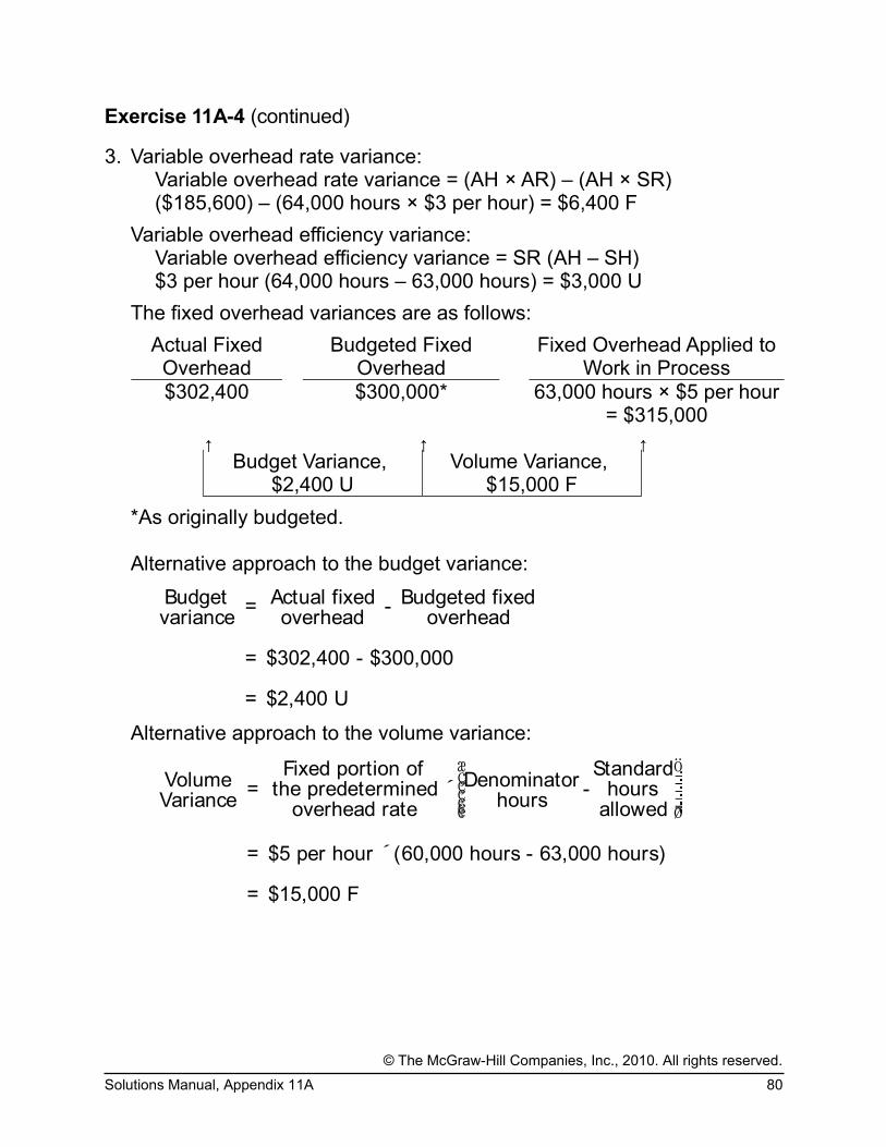
3. Variable overhead rate variance:Variable overhead rate variance = (AH × AR) – (AH × SR)($185,600) – (64,000 hours × $3 per hour) = $6,400 F
Variable overhead efficiency variance:Variable overhead efficiency variance = SR (AH – SH) $3 per hour (64,000 hours – 63,000 hours) = $3,000 U
The fixed overhead variances are as follows:
Actual FixedOverhead
Budgeted FixedOverhead
Fixed Overhead Applied toWork in Process
$302,400 $300,000* 63,000 hours × $5 per hour= $315,000
↑ ↑ ↑Budget Variance,
$2,400 UVolume Variance,
$15,000 F
*As originally budgeted.
Alternative approach to the budget variance:
Budget Actual fixed Budgeted fixed = - variance overhead overhead
= $302,400 - $300,000
= $2,400 U
Alternative approach to the volume variance:
æ ö÷ç ÷ç ÷ç ÷ç ÷÷çè ø
´
Fixed portion of StandardVolume Denominator = the predetermined - hoursVariance hoursoverhead rate allowed
= $5 per hour (60,000 hours - 63,000 hours)
= $15,000 F
© The McGraw-Hill Companies, Inc., 2010. All rights reserved.
Solutions Manual, Appendix 11A 80

Exercise 11A-5 (10 minutes)
Company A: This company has a favorable volume variance because the standard hours allowed for the actual production are greater than the denominator hours.
Company B: This company has an unfavorable volume variance because the standard hours allowed for the actual production are less than the denominator hours.
Company C: This company has no volume variance because the standard hours allowed for the actual production and the denominator hours are the same.
© The McGraw-Hill Companies, Inc., 2010. All rights reserved.
81 Managerial Accounting, 13th Edition

Exercise 11A-6 (15 minutes)
1. 9,500 units × 4 hours per unit = 38,000 hours.
2. and 3.
Actual FixedOverhead
Budgeted FixedOverhead
Fixed Overhead Applied toWork in Process
$198,700* $200,000 38,000 hours × $5 per hour*= $190,000
↑ ↑ ↑Budget Variance,
$1,300 FVolume Variance,
$10,000 U*
*Given.
4.
$200,000=
Denominator activity
= $5 per hour
Budgeted fixed overheadFixed element of the = predetermined overhead rate Denominator activity
Therefore, the denominator activity is: $200,000 ÷ $5 per hour = 40,000 hours.
© The McGraw-Hill Companies, Inc., 2010. All rights reserved.
Solutions Manual, Appendix 11A 82

Exercise 11A-7 (15 minutes)
1. 14,000 units produced × 3 MHs per unit = 42,000 MHs
2. Actual fixed overhead incurred.................. $267,000Add: Favorable budget variance............... 3,000 Budgeted fixed overhead cost................... $270,000
$270,000=
45,000 MHs
= $6 per MH
Budgeted fixed overhead Fixed element of the = predetermined overhead rate Denominator activity
3. Fixed portion of StandardVolume Denominator= the predetermined - hoursVariance hoursoverhead rate allowed
= $6 per MH (45,000 MHs - 42,000 MHs)
= $18,000 U
æ ö÷ç ÷ç ÷ç ÷ç ÷çè ø
Alternative solution to parts 1-3:
Actual FixedOverhead
Budgeted Fixed Overhead
Fixed Overhead Applied to Work in Process
$267,000* $270,0001 42,000 MHs2 × $6 per MH3
= $252,000
↑ ↑ ↑Budget Variance,
$3,000 F*Volume Variance,
$18,000 U1$267,000 + $3,000 = $270,000.214,000 units × 3 MHs per unit = 42,000 MHs3$270,000 ÷ 45,000 denominator MHs = $6 per MH
*Given.
© The McGraw-Hill Companies, Inc., 2010. All rights reserved.
83 Managerial Accounting, 13th Edition

Problem 11A-8 (30 minutes)
1. Direct materials, 3 yards × $4.40 per yard................................. $13.20Direct labor, 1 DLH × $12.00 per DLH....................................... 12.00Variable manufacturing overhead, 1 DLH × $5.00 per DLH*..... 5.00Fixed manufacturing overhead, 1 DLH × $11.80 per DLH**...... 11.80 Standard cost per unit............................................................... $42.00
* $25,000 ÷ 5,000 DLHs = $5.00 per DLH.** $59,000 ÷ 5,000 DLHs = $11.80 per DLH.
2. Materials variances:
Materials price variance = AQ (AP – SP) 24,000 yards ($4.80 per yard – $4.40 per yard) = $9,600 U
Materials quantity variance = SP (AQ – SQ) $4.40 per yard (18,500 yards – 18,000 yards*) = $2,200 U
*6,000 units × 3 yards per unit = 18,000 yards
Labor variances:
Labor rate variance = AH (AR – SR) 5,800 DLHs ($13.00 per DLH – $12.00 per DLH) = $5,800 U
Labor efficiency variance = SR (AH – SH)$12.00 per DLH (5,800 DLHs – 6,000 DLHs*) = $2,400 F
*6,000 units × 1 DLH per unit = 6,000 DLHs
© The McGraw-Hill Companies, Inc., 2010. All rights reserved.
Solutions Manual, Appendix 11A 84

Problem 11A-8 (continued)
3. Variable overhead variances:
Actual DLHs of Input, at the Actual Rate
Actual DLHs of Input, at the
Standard Rate
Standard DLHs Allowed for Output,
at the Standard Rate(AH × AR) (AH × SR) (SH × SR)$29,580 5,800 DLHs
× $5.00 per DLH6,000 DLHs
× $5.00 per DLH= $29,000 = $30,000
↑ ↑ ↑Rate Variance,
$580 UEfficiency Variance,
$1,000 FTotal Variance,
$420 F
Alternative solution for the variable overhead variances:
Variable overhead rate variance = (AH × AR) – (AH × SR)($29,580) – (5,800 DLHs × $5.00 per DLH) = $580 U
Variable overhead efficiency variance = SR (AH – SH) $5.00 per DLH (5,800 DLHs – 6,000 DLHs) = $1,000 F
Fixed overhead variances:
Actual FixedOverhead
Budgeted Fixed Overhead
Fixed OverheadApplied to
Work in Process$60,400 $59,000 6,000 DLHs
× $11.80 per DLH= $70,800
↑ ↑ ↑Budget Variance,
$1,400 UVolume Variance,
$11,800 F
© The McGraw-Hill Companies, Inc., 2010. All rights reserved.
85 Managerial Accounting, 13th Edition

Problem 11A-8 (continued)
Alternative approach to the budget variance:
Budget Actual fixed Budgeted fixed = -variance overhead overhead
= $60,400 - $59,000
= $1,400 U
Alternative approach to the volume variance:
æ ö÷ç ÷ç ÷ç ÷ç ÷÷çè ø
´
Fixed portion of StandardVolume Denominator= the predetermined - hoursVariance hoursoverhead rate allowed
= $11.80 per DLH (5,000 DLHs - 6,000 DLHs)
= $11,800 F
4. The choice of a denominator activity level affects standard unit costs in that the higher the denominator activity level chosen, the lower standard unit costs will be. The reason is that the fixed portion of overhead costs is spread over more units as the denominator activity rises.
The volume variance cannot be controlled by controlling spending. The volume variance simply reflects whether actual activity was greater than or less than the denominator activity. Thus, the volume variance is controllable only through activity.
© The McGraw-Hill Companies, Inc., 2010. All rights reserved.
Solutions Manual, Appendix 11A 86

Problem 11A-9 (45 minutes)
1. Direct materials price and quantity variances:
Materials price variance = AQ (AP – SP)64,000 feet ($8.55 per foot – $8.45 per foot) = $6,400 U
Materials quantity variance = SP (AQ – SQ) $8.45 per foot (64,000 feet – 60,000 feet*) = $33,800 U
*30,000 units × 2 feet per unit = 60,000 feet
2. Direct labor rate and efficiency variances:
Labor rate variance = AH (AR – SR)43,500 DLHs ($15.80 per DLH – $16.00 per DLH) = $8,700 F
Labor efficiency variance = SR (AH – SH)$16.00 per DLH (43,500 DLHs – 42,000 DLHs*) = $24,000 U
*30,000 units × 1.4 DLHs per unit = 42,000 DLHs
3. a. Variable overhead spending and efficiency variances:
Actual Hours of Input, at the Actual Rate
Actual Hours of Input, at the
Standard Rate
Standard Hours Allowed for Output,
at the Standard Rate(AH × AR) (AH × SR) (SH × SR)$108,000 43,500 DLHs
× $2.50 per DLH42,000 DLHs
× $2.50 per DLH= $108,750 = $105,000
↑ ↑ ↑Rate Variance,
$750 FEfficiency Variance,
$3,750 U
Alternative solution:
Variable overhead rate variance = (AH × AR) – (AH × SR) ($108,000) – (43,500 DLHs × $2.50 per DLH) = $750 F
Variable overhead efficiency variance = SR (AH – SH)$2.50 per DLH (43,500 DLHs – 42,000 DLHs) = $3,750 U
© The McGraw-Hill Companies, Inc., 2010. All rights reserved.
87 Managerial Accounting, 13th Edition

Problem 11A-9 (continued)
b. Fixed overhead budget and volume variances:
Actual FixedOverhead
Budgeted Fixed Overhead
Fixed Overhead Applied toWork in Process
$211,800 $210,000* 42,000 DLHs × $6 per DLH= $252,000
↑ ↑ ↑Budget Variance,
$1,800 UVolume Variance,
$42,000 F
*As originally budgeted. This figure can also be expressed as: 35,000 denominator DLHs × $6 per DLH = $210,000.
Alternative solution:
Budget variance:
Budget Actual fixed Budgeted fixed = -variance overhead overhead
= $211,800 - $210,000
= $1,800 U
Volume variance:
æ ö÷ç ÷ç ÷ç ÷ç ÷÷çè ø
´
Fixed portion of StandardVolume Denominator = the predetermined - hoursVariance hoursoverhead rate allowed
= $6.00 per DLH (35,000 DLHs - 42,000 DLHs)
= $42,000 F
© The McGraw-Hill Companies, Inc., 2010. All rights reserved.
Solutions Manual, Appendix 11A 88

Problem 11A-9 (continued)
4. The total of the variances would be:
Direct materials variances:Price variance................................................ $ 6,400 UQuantity variance........................................... 33,800 U
Direct labor variances:Rate variance................................................. 8,700 FEfficiency variance......................................... 24,000 U
Variable manufacturing overhead variances:Rate variance................................................. 750 FEfficiency variance......................................... 3,750 U
Fixed manufacturing overhead variances:Budget variance............................................. 1,800 UVolume variance............................................ 42,000 F
Total of variances.............................................. $18,300 U
Note that the total of the variances agrees with the $18,300 variance mentioned by the president.
It appears that not everyone should be given a bonus for good cost control. The materials quantity variance and the labor efficiency varianceare 6.7% and 3.6%, respectively, of the standard cost allowed and thus would warrant investigation.
The company’s large unfavorable variances (for materials quantity and labor efficiency) do not show up more clearly because they are offset by the favorable volume variance. This favorable volume variance is a result of the company operating at an activity level that is well above the denominator activity level used to set predetermined overhead rates. (The company operated at an activity level of 42,000 standard hours; thedenominator activity level set at the beginning of the year was 35,000 hours.) As a result of the large favorable volume variance, the unfavorable quantity and efficiency variances have been concealed in a small “net” figure. The large favorable volume variance may have been achieved by building up inventories.
© The McGraw-Hill Companies, Inc., 2010. All rights reserved.
89 Managerial Accounting, 13th Edition

Problem 11A-10 (45 minutes)
1. PZ297,500Total rate: = PZ8.50 per hour
35,000 hours
PZ87,500Variable rate: = PZ2.50 per hour
35,000 hours
PZ210,000Fixed rate: = PZ6.00 per hour
35,000 hours
2. 32,000 standard hours × PZ8.50 per hour = PZ272,000.
3. Variable overhead variances:
Actual Hours of Input, at the Actual Rate
Actual Hours of Input,at the Standard Rate
Standard Hours Allowed for Output, at
the Standard Rate(AH × AR) (AH × SR) (SH × SR)PZ78,000 30,000 hours ×
PZ2.50 per hour32,000 hours ×PZ2.50 per hour
= PZ75,000 = PZ80,000
↑ ↑ ↑Rate Variance,
PZ3,000 UEfficiency Variance,
PZ5,000 F
Alternative solution:
Variable overhead rate variance = (AH × AR) – (AH × SR)(PZ78,000) – (30,000 hours × PZ2.50 per hour) = PZ3,000 U
Variable overhead efficiency variance = SR (AH – SH) PZ2.50 per hour (30,000 hours – 32,000 hours) = PZ5,000 F
© The McGraw-Hill Companies, Inc., 2010. All rights reserved.
Solutions Manual, Appendix 11A 90

Problem 11A-10 (continued)
Fixed overhead variances:
Actual FixedOverhead
Budgeted FixedOverhead
Fixed Overhead Applied toWork in Process
PZ209,400 PZ210,000 32,000 hours ×PZ6 per hour = PZ192,000
↑ ↑ ↑Budget Variance,
PZ600 FVolume Variance,
PZ18,000 U
Alternative solution:
Budget variance:
Budget Actual fixed Budgeted fixed = -variance overhead overhead
= PZ209,400 - PZ210,000
= PZ600 F
Volume variance:
Fixed portion of StandardVolume Denominator= the predetermined - hoursVariance hoursoverhead rate allowed
= PZ6.00 per hour (35,000 hours - 32,000 hours)
= PZ18,000 U
æ ö÷ç ÷ç ÷ç ÷ç ÷÷çè ø
Verification:Variable overhead rate variance........ PZ 3,000 UVariable overhead efficiency variance 5,000 FFixed overhead budget variance........ 600 FFixed overhead volume variance....... 18,000 UUnderapplied overhead...................... PZ15,400 U
© The McGraw-Hill Companies, Inc., 2010. All rights reserved.
91 Managerial Accounting, 13th Edition

Problem 11A-10 (continued)
4. Variable overhead
Rate variance: This variance includes both price and quantity elements. The overhead spending variance reflects differences between actual and standard prices for variable overhead items. It also reflects differences between the amounts of variable overhead inputs that were actually used and the amounts that should have been used for the actual output of the period. Because the variable overhead spending variance is unfavorable, either too much was paid for variable overhead items or too many of them were used.
Efficiency variance: The term “variable overhead efficiency variance” is amisnomer, because the variance does not measure efficiency in the use of overhead items. It measures the indirect effect on variable overhead of the efficiency or inefficiency with which the activity base is utilized. In this company, the activity base is labor-hours. If variable overhead is really proportional to labor-hours, then more effective use of labor-hours has the indirect effect of reducing variable overhead. Because 2,000 fewer labor-hours were required than indicated by the labor standards, the indirect effect was presumably to reduce variable overhead spendingby about PZ5,000 (PZ2.50 per hour × 2,000 hours).
Fixed overhead
Budget variance: This variance is simply the difference between the budgeted fixed cost and the actual fixed cost. In this case, the variance is favorable which indicates that actual fixed costs were lower than anticipated in the budget.
Volume variance: This variance occurs as a result of actual activity beingdifferent from the denominator activity in the predetermined overhead rate. In this case, the variance is unfavorable, so actual activity was less than the denominator activity. It is difficult to place much of a meaningful economic interpretation on this variance. It tends to be large, so it often swamps the other, more meaningful variances if they are simply netted against each other.
© The McGraw-Hill Companies, Inc., 2010. All rights reserved.
Solutions Manual, Appendix 11A 92

Problem 11A-11 (45 minutes)
1. $600,000Total rate: = $10 per DLH
60,000 DLHs
$120,000Variable rate: = $2 per DLH
60,000 DLHs
$480,000Fixed rate: = $8 per DLH
60,000 DLHs
2. Direct materials: 3 pounds at $7 per pound............ $21Direct labor: 1.5 DLHs at $12 per DLH................... 18Variable overhead: 1.5 DLHs at $2 per DLH........... 3Fixed overhead: 1.5 DLHs at $8 per DLH............... 12 Standard cost per unit............................................. $54
3. a. 42,000 units × 1.5 DLHs per unit = 63,000 standard DLHs.
b. Manufacturing OverheadActual costs 606,500 Applied costs 630,000 *
Overapplied overhead 23,500
*63,000 standard DLHs × $10 per DLH = $630,000.
4. Variable overhead variances:
Actual Hours of Input, at the Actual Rate
Actual Hours of Input, atthe Standard Rate
Standard Hours Allowed for Output, at
the Standard Rate(AH × AR) (AH × SR) (SH × SR)$123,500 65,000 DLHs ×
$2 per DLH63,000 DLHs ×
$2 per DLH= $130,000 = $126,000
↑ ↑ ↑Rate Variance,
$6,500 FEfficiency Variance,
$4,000 U
© The McGraw-Hill Companies, Inc., 2010. All rights reserved.
93 Managerial Accounting, 13th Edition

Problem 11A-11 (continued)
Alternative solution:
Variable overhead rate variance = (AH × AR) – (AH × SR)($123,500) – (65,000 DLHs × $2 per DLH) = $6,500 F
Variable overhead efficiency variance = SR (AH – SH) $2 per DLH (65,000 DLHs – 63,000 DLHs) = $4,000 U
Fixed overhead variances:
Actual FixedOverhead
Budgeted Fixed Overhead
Fixed OverheadApplied to Work in Process
$483,000 $480,000* 63,000 DLHs × $8 per DLH= $504,000
↑ ↑ ↑Budget Variance,
$3,000 UVolume Variance,
$24,000 F
*Can be expressed as: 60,000 denominator DLHs × $8 per DLH = $480,000
Alternative solution:
Budget variance:
Budget Actual fixed Budgeted fixed = -variance overhead overhead
= $483,000 - $480,000
= $3,000 U
Volume variance:
æ ö÷ç ÷ç ÷ç ÷ç ÷÷çè ø
´
Fixed portion of StandardVolume Denominator = the predetermined - hoursVariance hoursoverhead rate allowed
= $8 per DLH (60,000 DLHs - 63,000 DLHs)
= $24,000 F
© The McGraw-Hill Companies, Inc., 2010. All rights reserved.
Solutions Manual, Appendix 11A 94

Problem 11A-11 (continued)
The company’s overhead variances can be summarized as follows:
Variable overhead:Rate variance................................... $ 6,500 FEfficiency variance........................... 4,000 U
Fixed overhead:Budget variance............................... 3,000 UVolume variance.............................. 24,000 F
Overapplied overhead—see part 3..... $23,500 F
5. Only the volume variance would have changed. It would have been unfavorable because the standard DLHs allowed for the year’s production (63,000 DLHs) would have been less than the denominator DLHs (65,000 DLHs).
© The McGraw-Hill Companies, Inc., 2010. All rights reserved.
95 Managerial Accounting, 13th Edition

Problem 11A-12 (45 minutes)
1. and 2. Per Direct Labor-HourVariable Fixed Total
Denominator of 30,000 DLHs:$135,000 ÷ 30,000 DLHs................... $4.50 $ 4.50 $270,000 ÷ 30,000 DLHs................... $9.00 9.00
Total predetermined rate...................... $13.50
Denominator of 40,000 DLHs:$180,000 ÷ 40,000 DLHs................... $4.50 $ 4.50 $270,000 ÷ 40,000 DLHs................... $6.75 6.75
Total predetermined rate...................... $11.25
3.Denominator Activity:
30,000 DLHsDenominator Activity:
40,000 DLHsDirect materials, 4 feet ×
$8.75 per foot................ $35.00 Same............................. $35.00Direct labor, 2 DLHs ×
$15 per DLH.................. 30.00 Same............................. 30.00Variable overhead, 2
DLHs × $4.50 per DLH.. 9.00 Same............................. 9.00Fixed overhead, 2 DLHs
× $9.00 per DLH............ 18.00 Fixed overhead, 2 DLHs
× $6.75 per DLH......... 13.50 Standard cost per unit...... $92.00 Standard cost per unit.... $87.50
4. a. 18,000 units × 2 DLHs per unit = 36,000 standard DLHs.
b. Manufacturing OverheadActual costs 446,400 Applied costs 486,000 *
Overapplied overhead 39,600
*36,000 standard DLHs × $13.50 predetermined rate per DLH = $486,000.
© The McGraw-Hill Companies, Inc., 2010. All rights reserved.
Solutions Manual, Appendix 11A 96

Problem 11A-12 (continued)
c. Variable overhead variances:
Actual DLHs of Input, at the Actual Rate
Actual DLHs of Input, at the
Standard Rate
Standard DLHs Allowed for Output,
at the Standard Rate(AH × AR) (AH × SR) (SH × SR)$174,800 38,000 DLHs ×
$4.50 per DLH36,000 DLHs ×$4.50 per DLH
= $171,000 = $162,000
↑ ↑ ↑Rate Variance,
$3,800 UEfficiency Variance,
$9,000 U
Alternative solution:Variable overhead rate variance = (AH × AR) – (AH × SR)($174,800) – (38,000 DLHs × $4.50 per DLH) = $3,800 U
Variable overhead efficiency variance = SR (AH – SH) $4.50 per DLH (38,000 DLHs – 36,000 DLHs) = $9,000 U
Fixed overhead variances:
Actual FixedOverhead
Budgeted FixedOverhead
Fixed Overhead Applied toWork in Process
$271,600 $270,000* 36,000 DLHs × $9 per DLH= $324,000
↑ ↑ ↑Budget Variance,
$1,600 UVolume Variance,
$54,000 F
*Can be expressed as: 30,000 denominator DLHs × $9 per DLH = $270,000.
© The McGraw-Hill Companies, Inc., 2010. All rights reserved.
97 Managerial Accounting, 13th Edition

Problem 11A-12 (continued)
Alternative solution:
Budget variance:
Budget Actual fixed Budgeted fixed = -variance overhead overhead
= $271,600 - $270,000
= $1,600 U
Volume variance:
æ ö÷ç ÷ç ÷ç ÷ç ÷÷çè ø
´
Fixed portion of StandardVolume Denominator = the predetermined - hoursVariance hoursoverhead rate allowed
= $9.00 per DLH (30,000 DLHs - 36,000 DLHs)
= $54,000 F
Summary of variances:Variable overhead rate variance.................. $ 3,800 UVariable overhead efficiency variance......... 9,000 UFixed overhead budget variance................. 1,600 UFixed overhead volume variance................ 54,000 FOverapplied overhead................................. $39,600 F
© The McGraw-Hill Companies, Inc., 2010. All rights reserved.
Solutions Manual, Appendix 11A 98

Problem 11A-12 (continued)
5. The major disadvantage of using normal activity is the large volume variance that ordinarily results. This occurs because the denominator activity used to compute the predetermined overhead rate is different from the activity level that is anticipated for the period. In the case at hand, the company has used a long-run normal activity figure of 30,000 DLHs to compute the predetermined overhead rate, whereas activity for the period was expected to be 40,000 DLHs. This has resulted in a largefavorable volume variance that may be difficult for management to interpret. In addition, the large favorable volume variance in this case has masked the fact that the company did not achieve the budgeted level of activity for the period. The company had planned to work 40,000DLHs, but managed to work only 36,000 DLHs (at standard). This unfavorable result is concealed due to using a denominator figure that isout of step with current activity.
On the other hand, using long-run normal activity as the denominator results in unit costs that are stable from year to year. Thus, management’s decisions are not clouded by unit costs that jump up and down as the activity level rises and falls.
© The McGraw-Hill Companies, Inc., 2010. All rights reserved.
99 Managerial Accounting, 13th Edition

Appendix 11BJournal Entries to Record Variances
Exercise 11B-1 (20 minutes)
1. The general ledger entry to record the purchase of materials for the month is:
Raw Materials (12,000 meters at $3.25 per meter)..................... 39,000
Materials Price Variance (12,000 meters at $0.10 per meter F)........ 1,200
Accounts Payable (12,000 meters at $3.15 per meter)............ 37,800
2. The general ledger entry to record the use of materials for the month is:
Work in Process (10,000 meters at $3.25 per meter)..................... 32,500
Materials Quantity Variance(500 meters at $3.25 per meter U)...................... 1,625
Raw Materials (10,500 meters at $3.25 per meter)............ 34,125
3. The general ledger entry to record the incurrence of direct labor cost for the month is:
Work in Process (2,000 hours at $12.00 per hour) 24,000Labor Rate Variance
(1,975 hours at $0.20 per hour U)....................... 395Labor Efficiency Variance
(25 hours at $12.00 per hour F)................. 300Wages Payable
(1,975 hours at $12.20 per hour)................ 24,095
© The McGraw-Hill Companies, Inc., 2010. All rights reserved.
Solutions Manual, Appendix 11B 100

Exercise 11B-2 (45 minutes)
1. a.Actual Quantity
of Input, at Actual Price
Actual Quantity of Input, at
Standard Price
Standard Quantity Allowed for Output, at Standard Price
(AQ × AP) (AQ × SP) (SQ × SP)10,000 yards ×$13.80 per yard
10,000 yards ×$14.00 per yard
7,500 yards* ×$14.00 per yard
= $138,000 = $140,000 = $105,000
↑ ↑ ↑Price Variance,
$2,000 F8,000 yards × $14.00 per yard
= $112,000
↑Quantity Variance,
$7,000 U
*3,000 units × 2.5 yards per unit = 7,500 yards
Alternatively, the variances can be computed using the formulas:
Materials price variance = AQ (AP – SP) 10,000 yards ($13.80 per yard – $14.00 per yard) = $2,000 F
Materials quantity variance = SP (AQ – SQ) $14.00 per yard (8,000 yards – 7,500 yards) = $7,000 U
© The McGraw-Hill Companies, Inc., 2010. All rights reserved.
101 Managerial Accounting, 13th Edition
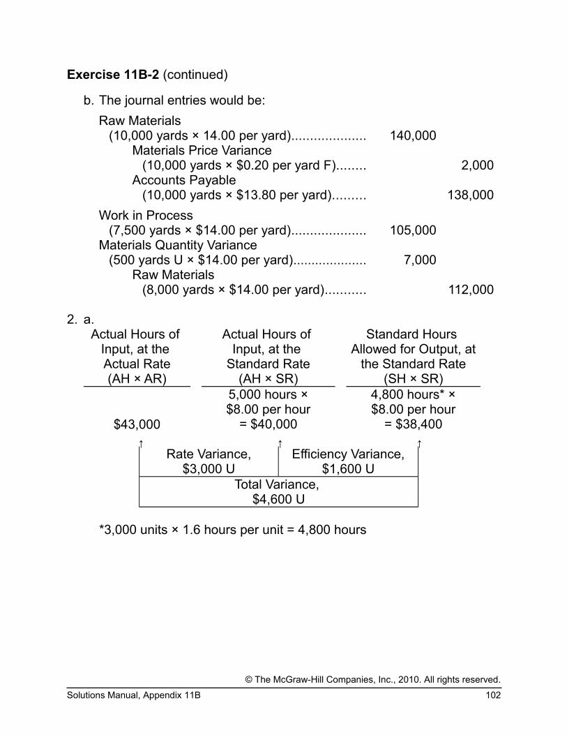
Exercise 11B-2 (continued)
b. The journal entries would be:
Raw Materials (10,000 yards × 14.00 per yard).................... 140,000
Materials Price Variance (10,000 yards × $0.20 per yard F)........ 2,000
Accounts Payable (10,000 yards × $13.80 per yard)......... 138,000
Work in Process (7,500 yards × $14.00 per yard).................... 105,000
Materials Quantity Variance (500 yards U × $14.00 per yard).................... 7,000
Raw Materials (8,000 yards × $14.00 per yard)........... 112,000
2. a.Actual Hours of
Input, at the Actual Rate
Actual Hours of Input, at the
Standard Rate
Standard Hours Allowed for Output, at
the Standard Rate(AH × AR) (AH × SR) (SH × SR)
5,000 hours ×$8.00 per hour
4,800 hours* ×$8.00 per hour
$43,000 = $40,000 = $38,400
↑ ↑ ↑Rate Variance,
$3,000 UEfficiency Variance,
$1,600 UTotal Variance,
$4,600 U
*3,000 units × 1.6 hours per unit = 4,800 hours
© The McGraw-Hill Companies, Inc., 2010. All rights reserved.
Solutions Manual, Appendix 11B 102

Exercise 11B-2 (continued)
Alternative Solution:
Labor rate variance = AH (AR – SR) 5,000 hours ($8.60 per hour* – $8.00 per hour) = $3,000 U
*$43,000 ÷ 5,000 hours = $8.60 per hour
Labor efficiency variance = SR (AH – SH) $8.00 per hour (5,000 hours – 4,800 hours) = $1,600 U
b. The journal entry would be:
Work in Process (4,800 hours × $8.00 per hour)........................ 38,400
Labor Rate Variance (5,000 hours × $0.60 per hour U)..................... 3,000
Labor Efficiency Variance (200 hours U × $8.00 per hour)........................ 1,600
Wages Payable (5,000 hours × $8.60 per hour)............... 43,000
3. The entries are: entry (a), purchase of materials; entry (b), issue of materials to production; and entry (c), incurrence of direct labor cost.
Raw Materials Work in Process(a) 140,000 (b) 112,000 (b) 105,000Bal.* 28,000 (c) 38,400
Accounts Payable Wages Payable(a) 138,000 (c) 43,000
Materials Price Variance Materials Quantity Variance(a) 2,000 (b) 7,000
Labor Rate Variance Labor Efficiency Variance(c) 3,000 (c) 1,600
*2,000 yards of material at a standard cost of $14.00 per yard
© The McGraw-Hill Companies, Inc., 2010. All rights reserved.
103 Managerial Accounting, 13th Edition

Problem 11B-3 (60 minutes)
1. a.
Actual Quantity of Input, at Actual Price
Actual Quantity of Input, at
Standard Price
Standard Quantity Allowed for Output, at
Standard Price(AQ × AP) (AQ × SP) (SQ × SP)
32,000 feet ×$4.80 per foot
32,000 feet ×$5.00 per foot
29,600 feet* ×$5.00 per foot
= $153,600 = $160,000 = $148,000
↑ ↑ ↑Price Variance,
$6,400 FQuantity Variance,
$12,000 UTotal Variance,
$5,600 U
*8,000 footballs × 3.7 ft. per football = 29,600 feet
Alternatively, the variances can be computed using the formulas:
Materials price variance = AQ (AP – SP)32,000 feet ($4.80 per foot – $5.00 per foot) = $6,400 F
Materials quantity variance = SP (AQ – SQ) $5.00 per foot (32,000 feet – 29,600 feet) = $12,000 U
b. Raw Materials (32,000 feet × $5.00 per foot). . 160,000Materials Price Variance
(32,000 feet × $0.20 per foot F)........... 6,400Accounts Payable
(32,000 feet × $4.80 per foot).............. 153,600
Work in Process (29,600 feet × $5.00 per foot)....................... 148,000
Materials Quantity Variance (2,400 feet U × $5.00 per foot)...................... 12,000
Raw Materials (32,000 feet × $5.00 per foot).............. 160,000
© The McGraw-Hill Companies, Inc., 2010. All rights reserved.
Solutions Manual, Appendix 11B 104

Problem 11B-3 (continued)
2. a.Actual Hours of
Input, at the Actual Rate
Actual Hours of Input, at the
Standard Rate
Standard Hours Allowed for Output,
at the Standard Rate(AH × AR) (AH × SR) (SH × SR)
6,400 hours* ×$8.00 per hour
6,400 hours ×$7.50 per hour
7,200 hours** ×$7.50 per hour
= $51,200 = $48,000 = $54,000
↑ ↑ ↑Rate Variance,
$3,200 UEfficiency Variance,
$6,000 FTotal Variance,
$2,800 F
* 8,000 footballs × 0.8 hours per football = 6,400 hours** 8,000 footballs × 0.9 hours per football = 7,200 hours
Alternatively, the variances can be computed using the formulas:
Labor rate variance = AH (AR – SR) 6,400 hours ($8.00 per hour – $7.50 per hour) = $3,200 U
Labor efficiency variance = SR (AH – SH) $7.50 per hour (6,400 hours – 7,200 hours) = $6,000 F
b. Work in Process (7,200 hours × $7.50 per hour). 54,000Labor Rate Variance
(6,400 hours × $0.50 per hour U)...................... 3,200Labor Efficiency Variance
(800 hours F × $7.50 per hour) ............... 6,000Wages Payable
(6,400 hours × $8.00 per hour)................ 51,200
© The McGraw-Hill Companies, Inc., 2010. All rights reserved.
105 Managerial Accounting, 13th Edition

Problem 11B-3 (continued)
3. Actual Hours of Input, at the Actual Rate
Actual Hours of Input, at the
Standard Rate
Standard Hours Allowed for Output,
at the Standard Rate(AH × AR) (AH × SR) (SH × SR)
6,400 hours ×$2.75 per hour
6,400 hours ×$2.50 per hour
7,200 hours ×$2.50 per hour
= $17,600 = $16,000 = $18,000
↑ ↑ ↑Rate Variance,
$1,600 UEfficiency Variance,
$2,000 FTotal Variance,
$400 F
Alternatively, the variances can be computed using the formulas:
Variable overhead rate variance = AH (AR – SR)6,400 hours ($2.75 per hour – $2.50 per hour) = $1,600 U
Variable overhead efficiency variance = SR (AH – SH)$2.50 per hour (6,400 hours – 7,200 hours) = $2,000 F
4. No. He is not correct in his statement. The company has a large, unfavorable materials quantity variance that should be investigated. Also, the overhead rate variance equals 10% of standard, which should also be investigated.
It appears that the company’s strategy to increase output by giving raises was effective. Although the raises resulted in an unfavorable rate variance, this variance was more than offset by a large, favorable efficiency variance.
© The McGraw-Hill Companies, Inc., 2010. All rights reserved.
Solutions Manual, Appendix 11B 106

Problem 11B-3 (continued)
5. The variances have many possible causes. Some of the more likely causes include the following:
Materials variances:
Favorable price variance: Good price, inferior quality materials, unusual discount due to quantity purchased, drop in market price, less costly method of freight, outdated or inaccurate standards.
Unfavorable quantity variance: Carelessness, poorly adjusted machines,unskilled workers, inferior quality materials, outdated or inaccurate standards.
Labor variances:
Unfavorable rate variance: Use of highly skilled workers, change in pay scale, overtime, outdated or inaccurate standards.
Favorable efficiency variance: Use of highly skilled workers, high-quality materials, new equipment, outdated or inaccurate standards.
Variable overhead variances:
Unfavorable rate variance: Increase in costs, waste, theft, spillage, purchases in uneconomical lots, outdated or inaccurate standards.
Favorable efficiency variance: Same as for labor efficiency variance.
© The McGraw-Hill Companies, Inc., 2010. All rights reserved.
107 Managerial Accounting, 13th Edition

Problem 11B-4 (75 minutes)
1. a. Before the variances can be computed, we must first compute the standard and actual quantities of material per hockey stick. The computations are:
Direct materials added to work in process (a). . $115,200Standard direct materials cost per foot (b)........ $3.00Standard quantity of direct materials (a) ÷ (b). . 38,400 feet
Standard quantity of direct materials (a)........... 38,400 feetNumber of sticks produced (b).......................... 8,000Standard quantity per stick (a) ÷ (b)................. 4.8 feet
Actual quantity of direct materials used per stick last year:4.8 feet + 0.2 feet = 5.0 feet.
With these figures, the variances can be computed as follows:
Actual Quantity of Input, at Actual Price
Actual Quantity of Input, at Standard Price
Standard Quantity Allowed for Output, at
Standard Price(AQ × AP) (AQ × SP) (SQ × SP)
60,000 feet ×$3.00 per foot
38,400 feet ×$3.00 per foot
$174,000 = $180,000 = $115,200
↑ ↑ ↑Price Variance,
$6,000 F40,000 feet* × $3.00 per foot
= $120,000
↑Quantity Variance,
$4,800 U
*8,000 units × 5.0 feet per unit = 40,000 feet
© The McGraw-Hill Companies, Inc., 2010. All rights reserved.
Solutions Manual, Appendix 11B 108

Problem 11B-4 (continued)
Alternatively, the variances can be computed using the formulas:
Materials price variance = AQ (AP – SP) 60,000 feet ($2.90 per foot* – $3.00 per foot) = $6,000 F
*$174,000 ÷ 60,000 feet = $2.90 per foot
Materials quantity variance = SP (AQ – SQ)$3.00 per foot (40,000 feet – 38,400 feet) = $4,800 U
b. Raw Materials (60,000 feet × $3.00 per foot)....... 180,000Materials Price Variance
(60,000 feet × $0.10 per foot F)................... 6,000Accounts Payable
(60,000 feet × $2.90 per foot)...................... 174,000
Work in Process (38,400 feet × $3.00 per foot). . . 115,200Materials Quantity Variance
(1,600 feet U × $3.00 per foot).......................... 4,800Raw Materials (40,000 feet × $3.00 per foot). 120,000
© The McGraw-Hill Companies, Inc., 2010. All rights reserved.
109 Managerial Accounting, 13th Edition

Problem 11B-4 (continued)
2. a. Before the variances can be computed, we must first determine the actual direct labor hours worked for last year. This can be done through the variable overhead efficiency variance, as follows:
Variable overhead efficiency variance = SR (AH – SH) $1.30 per hour × (AH – 16,000 hours*) = $650 U$1.30 per hour × AH – $20,800 = $650**$1.30 per hour × AH = $21,450 AH = $21,450 ÷ $1.30 per hour AH = 16,500 hours
* 8,000 units × 2.0 hours per unit = 16,000 hours** When used in the formula, an unfavorable variance is positive.
We must also compute the standard rate per direct labor hour. The computation is:
Labor rate variance = (AH × AR) – (AH × SR) $79,200 – (16,500 hours × SR) = $3,300 F$79,200 – 16,500 hours × SR = –$3,300*16,500 hours × SR = $82,500 SR = $82,500 ÷ 16,500 hours SR = $5.00 per hour
* When used in the formula, a favorable variance is negative.
© The McGraw-Hill Companies, Inc., 2010. All rights reserved.
Solutions Manual, Appendix 11B 110

Problem 11B-4 (continued)
Given these figures, the variances are:
Actual Hours of Input, at the Actual Rate
Actual Hours of Input,at the Standard Rate
Standard Hours Allowed for Output, at
the Standard Rate(AH × AR) (AH × SR) (SH × SR)
16,500 hours ×$5.00 per hour
16,000 hours ×$5.00 per hour
$79,200 = $82,500 = $80,000
↑ ↑ ↑Rate Variance,
$3,300 FEfficiency Variance,
$2,500 UTotal Variance,
$800 F
Alternatively, the variances can be computed using the formulas:
Labor rate variance = AH (AR – SR)16,500 hours ($4.80 per hour* – $5.00 per hour) = $3,300 F
*79,200 ÷ 16,500 hours = $4.80 per hour
Labor efficiency variance = SR (AH – SH)$5.00 per hour (16,500 hours – 16,000 hours) = $2,500 U
b. Work in Process (16,000 hours × $5.00 per hour)........................ 80,000
Labor Efficiency Variance (500 hours U × $5.00 per hour)......................... 2,500
Labor Rate Variance (16,500 hours × $0.20 per hour F)............... 3,300
Wages Payable (16,500 hours × $4.80 per hour).................. 79,200
© The McGraw-Hill Companies, Inc., 2010. All rights reserved.
111 Managerial Accounting, 13th Edition
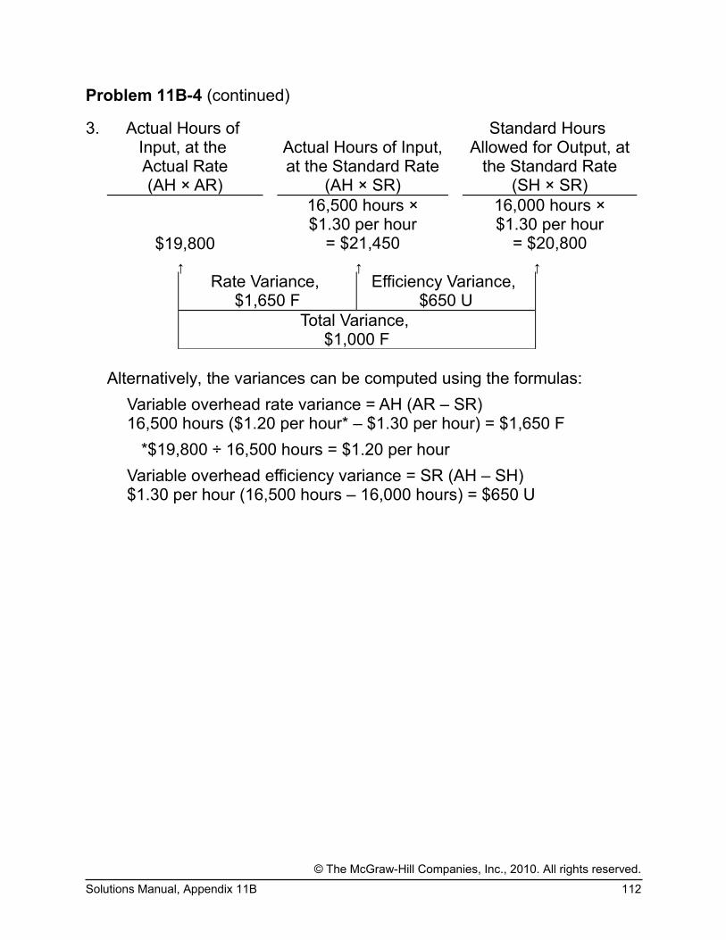
Problem 11B-4 (continued)
3. Actual Hours of Input, at the Actual Rate
Actual Hours of Input,at the Standard Rate
Standard Hours Allowed for Output, at
the Standard Rate(AH × AR) (AH × SR) (SH × SR)
16,500 hours ×$1.30 per hour
16,000 hours ×$1.30 per hour
$19,800 = $21,450 = $20,800
↑ ↑ ↑Rate Variance,
$1,650 FEfficiency Variance,
$650 UTotal Variance,
$1,000 F
Alternatively, the variances can be computed using the formulas:
Variable overhead rate variance = AH (AR – SR)16,500 hours ($1.20 per hour* – $1.30 per hour) = $1,650 F
*$19,800 ÷ 16,500 hours = $1.20 per hour
Variable overhead efficiency variance = SR (AH – SH)$1.30 per hour (16,500 hours – 16,000 hours) = $650 U
© The McGraw-Hill Companies, Inc., 2010. All rights reserved.
Solutions Manual, Appendix 11B 112

Problem 11B-4 (continued)
4. For materials:
Favorable price variance: Decrease in outside purchase price; fortunate buy; inferior quality materials; unusual discounts due to quantity purchased; less costly method of freight; inaccurate standards.
Unfavorable quantity variance: Inferior quality materials; carelessness; poorly adjusted machines; unskilled workers; inaccurate standards.
For labor:
Favorable rate variance: Unskilled workers (paid lower rates); piecework; inaccurate standards.
Unfavorable efficiency variance: Poorly trained workers; poor quality materials; faulty equipment; work interruptions; fixed labor and insufficient demand to fill capacity; inaccurate standards.
For variable overhead:
Favorable rate variance: Decrease in supplier prices; less usage of lubricants or indirect materials than planned; inaccurate standards.
Unfavorable efficiency variance: See comments under direct labor efficiency variance above.
5.Standard
Quantity orHours
Standard Priceor Rate
Standard Cost
Direct materials.............. 4.8 feet $3.00 per foot $14.40Direct labor.................... 2.0 hours $5.00 per hour 10.00Variable overhead.......... 2.0 hours $1.30 per hour 2.60 Total standard cost......... $27.00
Uploaded By Qasim Mughal
http://world-best-free.blogspot.com/
© The McGraw-Hill Companies, Inc., 2010. All rights reserved.
113 Managerial Accounting, 13th Edition