Stabilization of Energy Level Sets of UnderactuatedMechanical Systems Exploiting Impulsive BrakingNilay Kant 

Michigan State University College of EngineeringRanjan Mukherjee  ( mukherji@egr.msu.edu )

Michigan State University https://orcid.org/0000-0002-7211-1362Hassan K Khalil 

Michigan State University

Research Article

Keywords: energy level set , impulsive dynamics , underactuated mechanical systems

Posted Date: May 4th, 2021

DOI: https://doi.org/10.21203/rs.3.rs-445534/v1

License: This work is licensed under a Creative Commons Attribution 4.0 International License.  Read Full License

Noname manuscript No.(will be inserted by the editor)

Stabilization of Energy Level Sets of UnderactuatedMechanical Systems Exploiting Impulsive Braking

Nilay Kant · Ranjan Mukherjee · Hassan Khalil

Abstract Recent investigations of underactuated sys-

tems have demonstrated the benefits of control inputs

that are impulsive in nature. Here we consider the prob-lem of stabilization of energy level sets of underactu-

ated systems exploiting impulsive braking. We consider

systems with one passive degree-of-freedom (DOF) and

the energy level set is a manifold where the active co-ordinates are fixed and the mechanical energy equals

some desired value. A control strategy comprised of

continuous inputs and intermittent impulsive braking

inputs is presented. The generality of the approach is

shown through simulation of a three-DOF Tiptoebot;the feasibility of implementation of impulsive control

using standard hardware is demonstrated using a ro-

tary pendulum.

Keywords energy level set · impulsive dynamics ·

underactuated mechanical systems

1 INTRODUCTION

In many applications, such as legged locomotion [1, 2],

underactuated systems are required to undergo repeti-tive motion and orbital stabilization is the control ob-

jective. To achieve repetitive motion, geometric con-

N. KantMechanical Engineering Dept., Michigan State University, MI48824, USAE-mail: kantnila@msu.edu

R. MukherjeeMechanical Engineering Dept., Michigan State University, MI48824, USAE-mail: mukherji@egr.msu.edu

Hassan KhalilElectrical Engineering Dept., Michigan State University, MI48824, USAE-mail: khalil@msu.edu

straints are imposed on the generalized coordinates us-

ing the virtual holonomic constraint (VHC) approach

[3–6]. Orbital stabilization has also been used for swing-up control of underactuated systems with one passive

degree-of-freedom (DOF). Some examples include two-

DOF systems such as the pendubot [7], the acrobot [8],

the reaction-wheel pendulum [9], inverted pendulum ona cart [10,11], the rotary pendulum [12], and the three-

DOF gymnast robot [13]. These controllers stabilize an

energy level set that include the equilibrium, which is

typically unstable. Unlike the VHC approach, geomet-

ric constraints are not imposed; instead, the controllersare designed to pump energy in and out of the system

and converge the active DOFs to their desired config-

uration. Such control designs are typically based on a

Lyapunov-like function that is comprised of terms in-volving positions and velocities of the active DOFs and

the total mechanical energy of the system. Although

the structure of the Lyapunov-like function is identical,

the stability analysis is different for each system due to

the difference in the nature of their nonlinear dynamics.Despite the effectiveness of the individual controllers, a

general methodology for stabilizing an energy level set

does not exist. In this paper, we present a control strat-

egy for n-DOF underactuated systems with one passiveDOF based on continuous-time inputs and intermittent

impulsive braking inputs1.

Prior works on impulsive control [15–21] have been

theoretical in nature but in recent works [6,22–29], im-

pulsive inputs have been utilized for control of underac-

tuated systems in both simulations and experiments. Inexperiments, impulsive inputs have been implemented

in standard hardware using high-gain feedback [23,24],

dispelling the notion that impulsive inputs require large

1 Impulsive braking for control of the underctuated systemswas first proposed in [14] for swing-up of the pendubot.

2 Nilay Kant et al.

actuators and are impractical. A combination of contin-

uous and impulsive inputs was used recently for stabi-

lization of homoclinic orbits of two-DOF underactuated

systems [27]. This work provides a generalization of the

theory to n-DOF systems and experimental validation.In this paper, we present a control design for sta-

bilizing an energy level set for underactuated systems

with one passive revolute joint. The energy level set

is defined by fixed positions of the active coordinatesand a desired mechanical energy of the system. The

controller is comprised of continuous-time inputs and

impulsive braking inputs. At first, a general result for

underactuated systems is presented which shows that

an impulsive input causes an instantaneous jump inthe energy of the system; this jump is shown to be

explicitly dependent on the change in the active ve-

locities. This result is then used to show that impulsive

braking causes a negative jump in the energy of thesystem as well as in a Lyapunov-like function. Finally,

using a state-dependent impulsive dynamical system

model [16], we present sufficient conditions for stabi-

lization. To demonstrate the generality of our approach,

we demonstrate stabilization of energy level sets for thethree-DOF Tiptoebot [24] through simulations. Exper-

imental validation is carried out on a rotary pendulum

to show the applicability of our approach in real hard-

ware. The main contributions of this work are as fol-lows:

1. Our control design is applicable to a class of underac-

tuated systems; a majority of underactuated systems

investigated in the literature belong to this class.2. The stability analysis is presented for the general

case and it results in sufficient conditions that are

not restrictive and can be verified.

3. Experimental validation is provided.4. Impulsive braking is accomplished using a friction

brake; this eliminates the need for high-gain feed-

back [23] which may result in actuator saturation.

2 Problem Statement

Consider an n-DOF underactuated system with one

passive DOF. The generalized coordinates of the sys-

tem are denoted by q, q ,[

qT1 q2]T

, where q1 ∈ Rn−1

and q2 ∈ R are the coordinates associated with the

active and passive DOFs. Our control objective is to

stabilize the orbit defined by

(q1, q1, E) = (0, 0, Edes) (1)

where E is the total mechanical energy of the system

and is given by the relation

E(q, q) =1

2qTM(q) q + F(q) (2)

and Edes is the desired value of E. In (2), M(q) ∈ Rn×n

is the mass matrix, assumed to be positive definite, and

F(q) is the potential energy, assumed to be a smooth

function of q. The mass matrix is partitioned as

M(q) =

[

M11(q) M12(q)

MT12(q) M22(q)

]

(3)

where M11 ∈ R(n−1)×(n−1) and M22 ∈ R.

Assumption 1 The energy of the system is periodic in

the passive coordinate q2, such that E(q2+2π) = E(q2).

Remark 1 Assumption 1 is easily satisfied if the passive

DOF is a revolute joint.

Assumption 2 The elements of the mass matrix M(q)are bounded and the potential energy F(q) is lower bounded.

Remark 2 The boundedness property ofM(q) and F(q)

is satisfied for systems that have no prismatic joints.

3 Modeling of System Dynamics

3.1 Euler-Lagrange Equations

For our system described in section 2, the equations of

motion can be written as:

d

dt

(

∂L

∂q1

)

−

(

∂L

∂q1

)

= u

d

dt

(

∂L

∂q2

)

−

(

∂L

∂q2

)

= 0

(4)

where L(q, q) is the Lagrangian and u ∈ Rn−1 is the

vector of independent control inputs. Each element of

the vector u is a continuous function of time for all t ≥ 0

except at discrete instants t = τk, k = 1, 2, · · · , where

it is impulsive in nature. At t = τk, the impulsive inputvector has the form u(τk) = Ik δ(t−τk), where δ(t−τk)

is the Dirac measure at time τk and Ik ∈ Rn−1 is the

impulse of the impulsive input. The Lagrangian is

L(q, q) =1

2qTM(q) q −F(q) (5)

By substituting (3) in (5), the Lagrangian is written as

L(q, q) =1

2qT1 M11q1 +

1

2M22q

22 + qT1 M12q2 −F (6)

and by substituting (6) in (4), the equations of motion

become:

M11 q1 +M12 q2 + h1(q, q) = u (7a)

MT12 q1 +M22 q2 + h2(q, q) = 0 (7b)

Stabilization of Energy Level Sets of Underactuated Mechanical Systems Exploiting Impulsive Braking 3

where

h1 =M11 q1 + M12 q2 −1

2

[

∂

∂q1(M11 q1)

]

q1

−

[

∂(M12 q2)

∂q1

]

q1 −1

2

[

∂M22

∂q1

]T

q22 +

[

∂F

∂q1

]T

(8a)

h2 =M22 q2 + qT1 M12 −1

2qT1

[

∂(M11 q1)

∂q2

]

−1

2

[

∂M22

∂q2

]

q22 − qT1

[

∂(M12q2)

∂q1

]

+∂F

∂q2(8b)

Equations (7a) and (7b) can be rewritten in the form

q1 = A(q, q) +B(q)u (9a)

q2 = −(1/M22)[

MT12 {A(q, q) +B(q)u} + h2

]

(9b)

where

B(q) =[

M11 − (1/M22)M12 MT12

]−1(10)

A(q, q) = (1/M22)B(q) [M12 h2 − h1M22] (11)

Using properties of the mass matrixM(q) and the Schur

complement theorem [30], it can be shown that B(q) is

symmetric and positive-definite, i.e., B(q) = BT (q) >

0.

3.2 Effect of Impulsive Inputs

When the input u in (7a) is impulsive, it causes discon-

tinuous jumps in the velocities (q1, q2), while the co-

ordinates (q1, q2) remain unchanged. For the impulsive

input at t = τk, the jump in the velocities is computedby integrating (7) as follows [31]:

[

M11 M12

MT12 M22

] [

∆q1∆q2

]

=

[

Ik0

]

, Ik ,

∫ t+

k

t−

k

u(tk) dt

In the above equation, ∆q1 and ∆q2 are defined as

∆q1 , (q+1 − q−1 ), ∆q2 , (q+2 − q−2 )

where q− , q(τ−k ) and q+ , q(τ+k ) denote the general-ized velocities immediately before and after application

of the impulsive inputs. Since the system is underactu-

ated, the jump in q2 is dependent on the jumps in q1;

this dependence is described by the one-dimensional im-pulse manifold [23] or impulse line, obtained from the

equation above:

q+2 = q−2 − (1/M22)MT12(q

+1 − q−1 ) (12)

The kinetic energy undergoes an instantaneous change

due to jumps in the generalized velocities. This change

is also equal to the change in the total mechanical en-ergy of the system since the potential energy is only a

function of the generalized coordinates. A formal state-

ment of this result is provided next.

Lemma 1 For the dynamical system in (7), the jump

in the total mechanical energy due to application of an

impulsive input is given by

∆E , (E+ − E−) =1

2q+

T

1 B−1(q) q+1 −1

2q−

T

1 B−1(q) q−1

(13)

where E− and E+ are the energies immediately before

and after application of the impulsive input.

Proof: See section 8.1 of Appendix.

Remark 3 The proof of Lemma 1 is provided for the

general case where the number of active and passive

DOFs are (n−m) and m, respectively. This general re-sult indicates that the change in mechanical energy due

to an impulsive input depends only on the velocities of

the active DOFs immediately before and after applica-

tion of the input. The result is analogous to the pas-sivity property for the continuous-time case [32], where

the power input to the system is the inner product of

the velocities of the active DOFs and control inputs. It

is important to note that results similar to Lemma 1

appeared earlier in [33].

Impulsive braking results in q+1 = 0. Thus it follows

from Lemma 1 that impulsive braking results in a loss

of mechanical energy, given by the expression

∆E = −1

2q−

T

1 B−1(q) q−1 (14)

We now state an important result related to impulsive

braking.

Lemma 2 Consider the scalar function

V =1

2

[

qT1 Kp q1 + qT1 Kd q1 +Ke(E − Edes)2]

(15)

where Kp and Kd are diagonal positive definite con-

stant matrices and Ke is a positive constant. Impulsive

braking results in a discontinuous jump in the function

given by

∆V , (V + − V −)

= −1

2q−

T

1

[

1

4

{

Ke q−

T

1 B−1(q) q−1

}

B−1(q)

+Kd +Ke(E+ − Edes)B

−1(q)

]

q−1

(16)

where V − and V + are values of the function immedi-

ately before and after impulsive braking. Furthermore, if[

Kd +Ke(E+ − Edes)B

−1(q)]

is positive definite, then∆V ≤ 0, and ∆V = 0 if and only if q−1 = 0.

Proof: See section 8.2 of Appendix.

4 Nilay Kant et al.

3.3 Impulsive Dynamical Model

To stabilize the orbit in (1), we propose a control strat-egy comprised of continuous and impulsive inputs. The

impulsive inputs will be used for impulsive braking of

the active coordinates, i.e., q+1 = 0. As a result, the

change in the velocities can be obtained using (12) as

follows:

∆q1 = 0− q−1 = −q−1

∆q2 = q+2 − q−2 = (1/M22)MT12 q

−

1

(17)

In addition to the impulsive braking inputs, we will

reset the passive coordinate q2 periodically to confine

it to the compact set [−3π/2, π/2]2. To describe the

dynamics of our system, we adopt the state-dependentimpulsive dynamical model in [16, pg.20]:

x(t) = fc[x(t)], x(0) = x0, x(t) /∈ Z (18a)

∆x(t) = fd[x(t)], x(t) ∈ Z (18b)

where Z defines the set where the impulsive inputs are

applied and/or periodic resetting occurs. For our sys-

tem,

x(t) , [qT1 q2 qT1 q2]T ∈ D ⊆ R2n

∆x(t) , x(t+)− x(t−)

In the above expression, D is the open set where q2 ∈

(a, b), a < −3π/2, b > π/2, and x(t−), x(t+) are the val-ues of the state variables immediately before and after

application of impulsive inputs or coordinate resetting.

Using (9), (12) and (17), it can be shown

fc =

q1q2

A(q, q) + B(q)u

−(1/M22)[

MT12 {A(q, q) +B(q)u}+ h2

]

(19)

fd =

[

0 0 −q−1 (1/M22)MT12 q

−

1

]T:x(t) ∈ Z1

[

0 2π 0 0]T

:x(t) ∈ Z2[

0 −2π 0 0]T

:x(t) ∈ Z3

(20)

Z = Z1∪Z2∪Z3, Z1 is the set where impulsive brakinginputs are applied (to be defined in Theorem 2 where

the control design will be presented), and Z2 , {q2 =

−3π/2, q2 < 0} and Z3 , {q2 = π/2, q2 > 0} are the

sets where coordinate resetting occurs.

We assume existence and uniqueness of the solutionof (18) to exclude the possibility of complex phenom-

ena such as Zeno switching [16, 21]. Simulations and

experimental results presented later will validate this

assumption.

2 This choice of the compact set is not unique.

4 Control Design

4.1 Main Result

For the objective in (1), we propose a control design

comprised of continuous and intermittent impulsive brak-

ing inputs3. Theorem 2 provides the design of the con-tinuous controller and defines the set Z1, where impul-

sive braking is applied. The proof of Theorem 2 is based

on a Lyapunov-like function. The continuous controller

is invoked as long as the derivative of the Lyapunov-like function is negative semi-definite; when this con-

dition is not satisfied, impulsive braking is applied to

produce negative jumps in the Lyapunov-like function.

Before stating Theorem 2, we present an invariant set

theorem [16, pg.38] that will be used in the proof ofTheorem 2 and state one Assumption.

Theorem 1 [16, pg.38] Consider the impulsive dy-

namical system given by (18), assume that Dc ⊂ D is acompact positively invariant set with respect (18), and

assume that there exists a continuously differentiable

function W : D → R such that

[∂W (x)/∂x] fc(x) ≤ 0, x ∈ Dc, x /∈ Z (21a)

W (x+ fd(x)) ≤ W (x), x ∈ Dc, x ∈ Z (21b)

Let R , {x ∈ Dc : x /∈ Z, [∂W (x)/∂x] fc(x) = 0} ∪

{x ∈ Dc : x ∈ Z,W (x + fd(x)) = W (x)} and let M

denote the largest invariant set contained in R. If x0 ∈

Dc, then x(t) → M as t → ∞.

Assumption 3 For the system in (7) subjected to con-

tinuous control, q2 is constant if q1 and u are identically

zero.

Remark 4 Assumption 3 implies that the active and

passive generalized coordinates are dynamically cou-

pled. Due to this coupling, the active generalized co-

ordinates cannot be held stationary by constant gener-

alized forces when the passive generalized coordinate isnon-stationary. The existence of such coupling has been

verified for an inverted pendulum on a cart [27], rotary

pendulum [34], pendubot, acrobot, and reaction-wheel

pendulum; in this paper it is shown for the tiptoebot.

Theorem 2 For the impulsive dynamical system de-

fined by (18), (19) and (20), and x0 ∈ D such that

−3π/2 < q2(0) < π/2 (22)

3 It is assumed that the active DOFs will have a frictionbrake such that they can be stopped instantaneously.

Stabilization of Energy Level Sets of Underactuated Mechanical Systems Exploiting Impulsive Braking 5

the following choice of control design:

u = − [(Kd +Kc)B(q) +Ke (E − Edes) I]−1 ×

[Kp q1 + (Kd +Kc)A(q, q)] (23a)

Z1 = {x(t) | [A(q, q) +B(q)u]TKc q1 ≤ 0, q1 6= 0}

(23b)

where I is the identity matrix and Kc is a diagonalpositive-definite matrix, guarantees asymptotic stability

of the orbit in (1) if the gain matrices Kp, Kd and Ke

satisfy the following conditions:

(i)[

Kd +Ke(E − Edes)B−1(q)

]

is positive definite forall q and q,

(ii) If q∗1 and q∗2 are constant values of q1 and q2, then

the following system of equations:

[

∂F

∂q1

]T

q=q∗

= −Kp q

∗

1

Ke [F(q∗)− Edes][

∂F

∂q2

]

q=q∗

= 0

yields a finite number of solutions with q∗1 = 0,

and

(iii) For all possible solutions of q∗2 obtained from (ii)

and for the function V in (15), the following in-equality is satisfied

V (t=0) < min{V | q1 = 0, q1 = 0, E ∈ SE\{Edes}}

where SE is the set of values of E evaluated at

q1 = 0, q2 = q∗2 , q = 0.

Proof: Consider the Lyapunov-like function V de-fined in (15); V is zero on the orbit defined in (1) and

positive everywhere else. The time derivative of V is

V = qT1 Kp q1 + qT1 Kd q1 +Ke(E − Edes)E

=[

qT1 Kp + qT1 Kd +Ke(E − Edes)uT]

q1(24)

where E = uT q1 follows from the passivity property of

underactuated Euler-Lagrange systems - see [32]4 and

proposition 2.5 of [35]. By substituting q1 from (9a) in

(24) and using the symmetry of B(q), we get

V =[

qT1 Kp +ATKd

+uT B{

Kd +Ke(E − Edes)B−1

}]

q1(25)

The following choice of u

uT = −[

qT1 Kp +ATKd + qT1 Kc

]

×[

B{

Kd +Ke(E − Edes)B−1

}]

−1,

(26)

4 The proof of the passivity property follows from the factthat the matrix [M − 2C] is skew-symmetric for our choice ofgeneralized coordinates.

which is well defined based on condition (i), results in

V = −qT1 Kc q1 (27)

Substitution of (9a) in (26) followed by algebraic ma-

nipulation gives the expression for u in (23a). Substitu-

tion of (9a) in (27) gives

V = − [A(q, q) +B(q)u]TKc q1 (28)

Based on the expression of V , three cases may arise:

case (a): if [A+Bu]TKc q1 > 0, then V < 0,

case (b): if [A+Bu]TKc q1 ≤ 0, q1 6= 0, then x ∈ Z1

and impulsive braking is applied - see (23b).Since condition (i) is satisfied, Lemma 2 indi-

cates that V undergoes a discontinuous change

∆V , where ∆V < 0, and

case (c): if q1 = 0, then V = 0.

For case (b), impulsive braking results in q1 = 0 at t+

and the trajectories of the system leave Z1. If q1 ≡ 0 for

all t > t+, the trajectories of the system remain outsideZ1 and V ≡ 0. If q1 6≡ 0 for t > t+, V decreases since

(27) implies

V (t+) = 0, V (t+) = −qT1 (t+)Kc q1(t

+) < 0

⇒ V (τ) < 0, τ ∈ (t+, t+ + ε)

for some ε > 0 since Kc is positive-definite and q1 6= 0.

Case (c) implies that either q1 ≡ 0 ⇒ V ≡ 0, or q1 6≡ 0and V continues to decrease again; this follows from our

discussion of the nature of trajectories after impulsive

braking. Cases (a), (b) and (c) imply that for t > 0,

V (t) ≤ V (0) , c and therefore the set

Dc , {V ≤ c} ∩ {−3π/2 ≤ q2 ≤ π/2}

is positively invariant.

Cases (a), (b) and (c) together satisfy the conditions

in Theorem 1 with Dc defined above and W (x) = V (x).

Since (b) implies ∆V < 0, {x ∈ Dc : x ∈ Z, ∆V = 0} is

an empty set. Therefore, x(t) → M ⊂ R = {x ∈ Dc :x /∈ Z, V = 0} as t → ∞. From case (c), V = 0 implies

q1 = 0 and thus R = {x ∈ Dc : q1 ≡ 0}. In R, q1 = 0.

Substitution of q1 = 0 in (9a) and (26) yields

uT = −ATB−1 (29a)

uTBKd = −Ke(E − Edes)uT − qT1 Kp −ATKd (29b)

Substitution of (29a) into (29b) gives

uTKe (E − Edes) + qT1 Kp = 0 (30)

The definition of R in Theorem 1 implies V is constant

in R. Also, q1 is constant and q1 = 0 in R. Therefore,from the definition of V in (15), we can claim that E

is constant in R. Let q∗1 and E∗ be the constant values

of q1 and E. We now discuss two cases that can arise:

6 Nilay Kant et al.

case 1: If E∗ = Edes, we have q∗1 = 0 from (30). This

implies that M is the orbit in (1).

case 2: if E∗ 6= Edes, we get from (30)

u , u∗ = −Kp q

∗

1

Ke(E∗ − Edes)(31)

where u∗ is the constant value of the continuous

control in R.

For case 2, both q1 and u are constants. Therefore,based on Assumption 3, we claim q2 = q∗2 is a con-

stant. It follows from (2) that E∗ = F(q∗). Using (7)

and (8), we can show that the trajectories in R satisfy

[

∂F

∂q1

]T

q=q∗

= u∗,

[

∂F

∂q2

]

q=q∗

= 0

Substituting the expression for u∗ from (31) in the above

equation along with E∗ = F(q∗), we can use condition(ii) to claim q∗1 = 0. Using (15) and cases (a) and (b),

we can claim that as t → ∞, V → V ∗, where

V ∗ =1

2Ke(E

∗ − Edes)2 ≤ V (t = 0)

where E∗ ∈ SE . Since V ∗ ≤ V (t = 0), we can claim

using condition (iii) that E∗ = Edes, i.e., V∗ = 0. Thus

the largest invariant set M is the orbit defined in (1).This concludes the proof.

4.2 Choice of Controller Gains

It can be easily shown that condition (i) in Theorem 2

is satisfied if

(1/Ke)λmin(Kd) > [Edes −min(F)]λmax[B−1(q)]

where λmin(Kd) and λmax[B−1(q)] are the minimum

and maximum eigenvalues ofKd and [B−1(q)]. Assump-

tion 2 implies λmax[B−1(q)] and min(F) exist and there-

fore Kd and Ke can always be chosen to satisfy condi-tion (i).

For the choice of Ke satisfying condition (i), Kp hasto be chosen to satisfy condition (ii). Although we do

not prove that condition (ii) can be simultaneously sat-

isfied for the general case, several combinations of gains

(Kp,Kd,Ke) were found to exist for the inverted pen-

dulum on a cart [27]. The authors have independentlyverified that condition (ii) can be easily satisfied for sev-

eral other underactuated mechanical systems, namely,

the pendubot, the acrobot, and the reaction-wheel pen-

dulum. It is shown in this paper that conditions (i) and(ii) can be simultaneously satisfied for the three-DOF

Tiptoebot and the rotary pendulum. These examples

indicate that condition (ii) is not restrictive.

Once the controller gains Kp, Kd and Ke have been

chosen to satisfy conditions (i) and (ii) in Theorem 2,

condition (iii) imposes no additional restrictions on the

gains but simply provides an estimate of the region of

attraction of the orbit. Since Kc does not appear inconditions (i)-(iii), it can be chosen without restriction.

5 Illustrative Example - The Tiptoebot

5.1 System Description

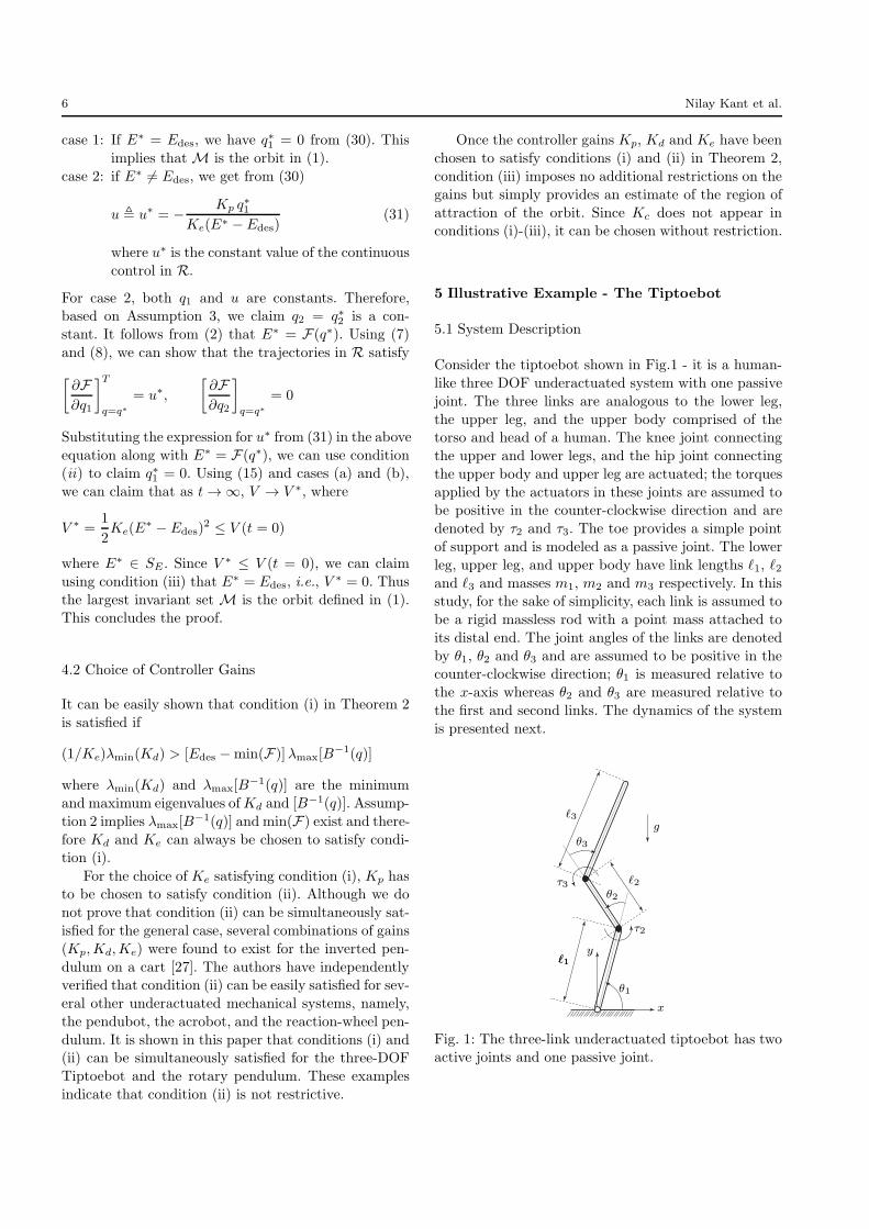
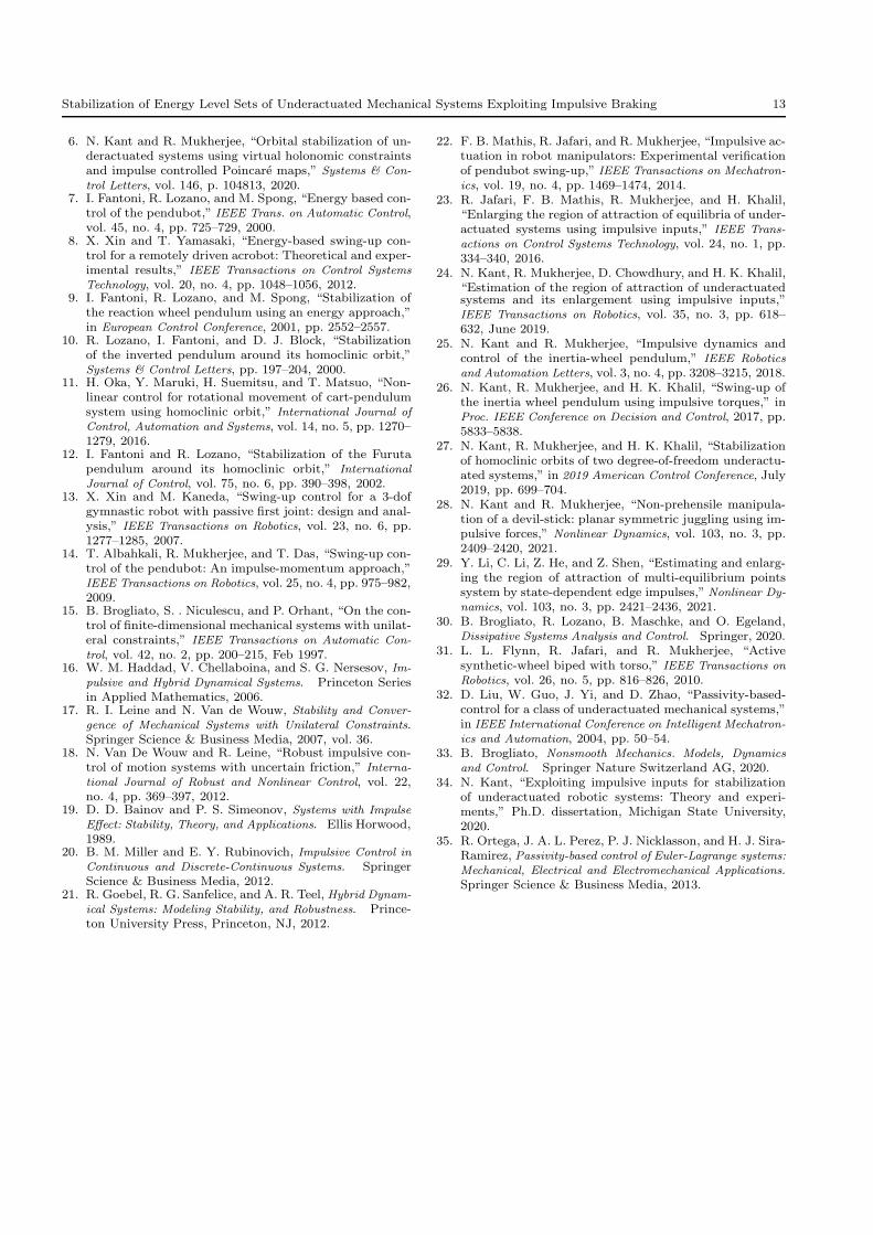
Consider the tiptoebot shown in Fig.1 - it is a human-

like three DOF underactuated system with one passive

joint. The three links are analogous to the lower leg,

the upper leg, and the upper body comprised of thetorso and head of a human. The knee joint connecting

the upper and lower legs, and the hip joint connecting

the upper body and upper leg are actuated; the torques

applied by the actuators in these joints are assumed tobe positive in the counter-clockwise direction and are

denoted by τ2 and τ3. The toe provides a simple point

of support and is modeled as a passive joint. The lower

leg, upper leg, and upper body have link lengths ℓ1, ℓ2and ℓ3 and masses m1, m2 and m3 respectively. In thisstudy, for the sake of simplicity, each link is assumed to

be a rigid massless rod with a point mass attached to

its distal end. The joint angles of the links are denoted

by θ1, θ2 and θ3 and are assumed to be positive in thecounter-clockwise direction; θ1 is measured relative to

the x-axis whereas θ2 and θ3 are measured relative to

the first and second links. The dynamics of the system

is presented next.

ℓ1ℓ1

ℓ2

ℓ3

θ1

θ2

θ3

τ2

τ3

x

y

g

Fig. 1: The three-link underactuated tiptoebot has twoactive joints and one passive joint.

Stabilization of Energy Level Sets of Underactuated Mechanical Systems Exploiting Impulsive Braking 7

5.2 Tiptoebot Dynamics and Control Objective

Using the following definition for the joint angles

qT1 = [θ2 θ3 ]T , q2 = θ1 (32)

the dynamics of the tiptoebot can be expressed in the

form of (7); the components of mass matrix in (3) are

M11 =

[

α2+α3+2α5 cos θ3 α3+α5 cos θ3α3+α5 cos θ3 α3

]

M12 =

[

α2+α3+α4 cos θ2+2α5 cos θ3+α6 cos(θ2+θ3)

α3+α5 cos θ3+α6 cos(θ2+θ3)

]

M22 = α1+α2+α3

+ 2 [α4 cos θ2 + α5 cos θ3+α6 cos(θ2+θ3)]

(33)

where αi, i = 1, 2, · · · , 6, are lumped parameters, de-

fined as follows:

α1 , m1(ℓ21 + ℓ22 + ℓ23), α2 , (m2 +m3)ℓ

22

α3 , m3ℓ23, α4 , m2ℓ1ℓ2 +m3ℓ1ℓ2

α5 , m3ℓ2ℓ3, α6 , m3ℓ1ℓ3

(34)

The sum of Coriolis, centrifugal and gravitational force

terms, h1 and h2, can be obtained using (8), where F(q)

has the expression

F =β1 sin θ1 + β2 sin(θ1 + θ2) + β3 sin(θ1 + θ2 + θ3)

β1 , (m1 +m2 +m3)ℓ1 g

β2 , (m2 +m3)ℓ2 g, β3 , m3ℓ3 g

(35)

The control input is defined as u = [τ2 τ3]T . In the

compact set θ1 ∈ [−3π/2, π/2], as defined in section 3.3,

the upright equilibrium configuration of the tiptoebot

is defined by

θ1 = −3π/2 or π/2,[

θ2 θ3 θ1 θ2 θ3]

=[

00000]

is unstable, but can be stabilized, by a linear controller,

for example. The stabilized equilibrium will typically

have a finite region of attraction; therefore, to stabilize

from an arbitrary initial configurations, we first use thecontroller in section 3 to stabilize an energy level set

that intersects the region of attraction. The obvious

choice for such a level set is the one where Edes equals

the potential energy of the system at the equilibrium.

Substitution of θ1 = −3π/2 or π/2 and θ2 = θ3 = 0 in(35) yields Edes = β1 + β2 + β3. The control objective

in (1) can therefore be written as

θ2 = θ3 = 0, θ2 = θ3 = 0, Edes = (β1 + β2 + β3) (36)

The feasibility of our control design is discussed next.

5.3 Selection of Controller Gains

The initial configuration of the tiptoebot is taken as

[θ1 θ2 θ3 θ1 θ2 θ3 ] = [0π π 000 ] (37)

In this configuration, the tiptoebot is coiled up: the first

link is horizontal, the second link folds back on the firstlink, and the third link folds back on the second link.

The links were chosen to have the same mass m1 =

m2 = m3 = 0.1 kg and the same length ℓ1 = ℓ2 = ℓ3 =

0.6 m. For this choice of mass and length parameters,

the lumped parameters of the tiptoebot, defined in (34)and (35), are provided in Table 1 below:

Table 1: Tiptoebot lumped parameters in SI units

α1 0.108 α4 0.072 β1 1.764

α2 0.072 α5 0.036 β2 1.176

α3 0.036 α6 0.036 β3 0.588

The passive joint of the tiptoebot is revolute and there-

fore assumption 1 hold good. From the expressions in

(33) and (35), it can be verified that assumption 2 holdsgood. Assumption 3 also holds good - this is discussed

in the Appendix 8.3.

The following choice of gains satisfy condition (i)

and (ii):

Kp =

[

70 00 70

]

, Kd =

[

2.8 00 2.8

]

, Ke = 2.2 (38)

Condition (ii) results in θ∗2 = θ∗3 = 0, which upon sub-

stitution in (7b) and (8b) yields

∂F

∂q2= 0 ⇒ cos θ∗1 = 0 (39)

From section 3.3 we know that q2 lies in the compact

set [−3π/2, π/2]. Thus θ1 lies in the same compact set- see (32). In this set, the possible solutions of (39) are

θ∗1 = {−3π/2,−π/2, π/2}. For θ∗1 = −3π/2 or π/2, and

θ∗2 = θ∗3 = 0, we know that E = Edes. Therefore, to

satisfy condition (iii), we use θ∗1 = −π/2; this results inthe following inequality

V (t = 0) < 2Ke [E(q∗1 = 0, q∗2 = −π/2)− Edes]2

= 2Ke(β1 + β2 + β3)2

For the initial configuration in (37), Ke in (38) satisfies

the inequality above. The matrix Kc was chosen as

Kc =

[

1.2 00 1.2

]

(40)

8 Nilay Kant et al.

5.4 Simulation Results

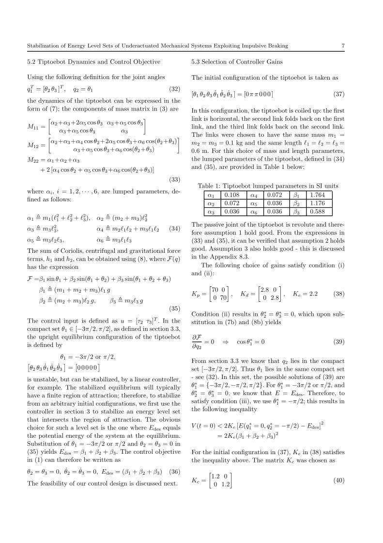
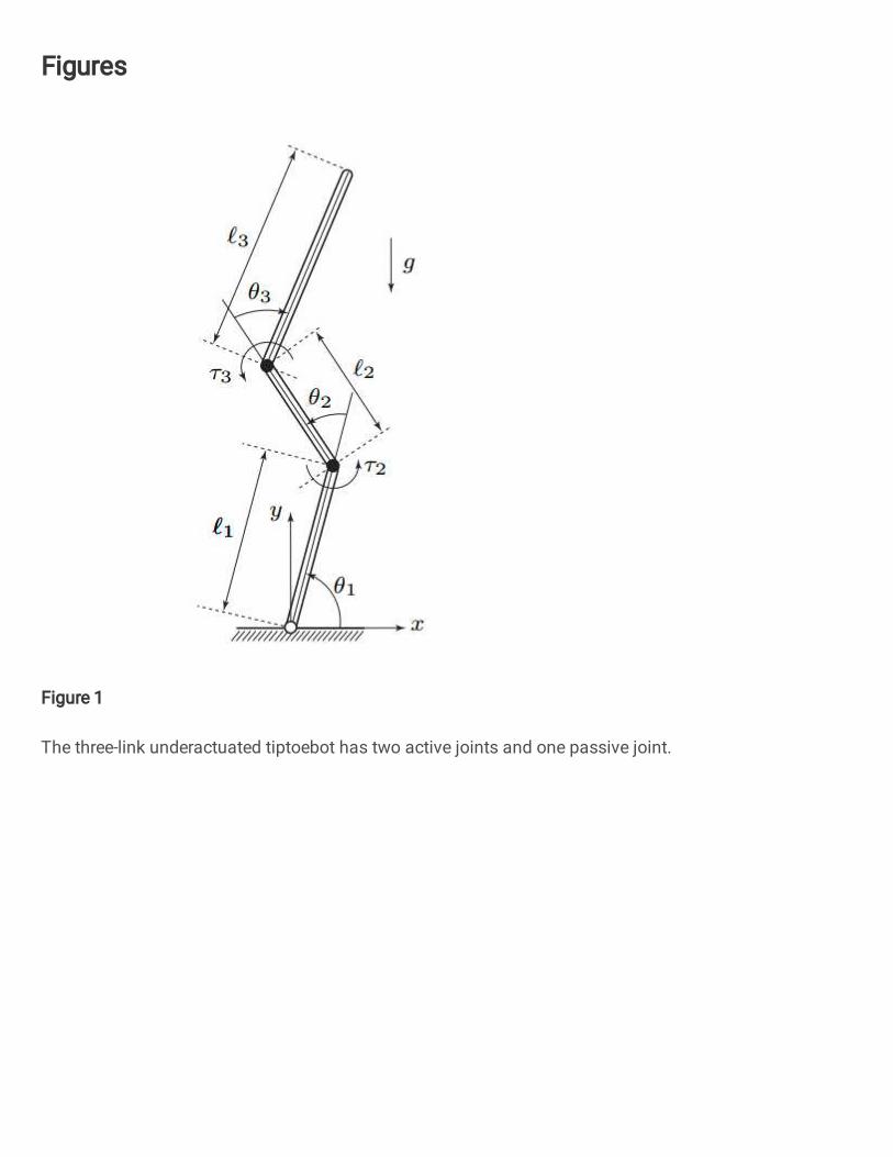
For the initial configuration in (37) and controller gains

in (38) and (40), the simulation results are shown in

Figs.2 and 3. The effect of impulsive braking can be seenin Figs.2 (d) and (f), where θ2 and θ3 (the velocities of

the active joints) jump to zero on multiple occasions.

Each impulsive braking also results in a negative jump

in the mechanical energy (follows from Lemma 1) whichcan be seen in Fig.2 (b). Since impulsive inputs cause

no jumps in the joint angles, there is no change in θ1,

θ2 and θ3 at the time of impulsive braking - see Figs.2

(a), (c) and (e). In Fig.2 (a), θ1 never leaves the set

[−3π/2, π/2] and therefore virtual impulsive inputs arenot applied.

While impulsive brakings cause negative jumps inthe total energy E, the continuous-time controller in

(23a) adds energy to the system; together, they con-

verge the energy to the desired values Edes - see Fig.2

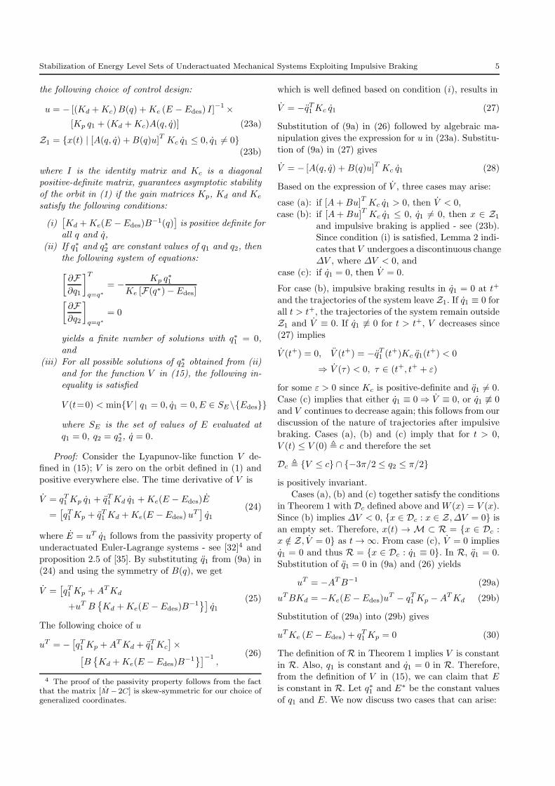
(b). The phase portrait of the passive joint is shownin Fig.3 (a). The jumps in the phase portrait (verti-

cal drops in θ1, twice) is due to impulsive braking. The

variation of the Lyapunov-like function V with time is

shown in Fig.3 (b) - it can be seen that V decreases

monotonically due to the action of the continuous-timecontroller and undergoes negative jumps intermittently

due to impulsive brakings. The continuous controller

and impulsive brakings work together to converge V to

zero.

The gain matrices in (38) and (40) were chosen such

that convergence to the desired level set is fast. The

simulation results indicate that the system trajectories

0.0

3.0

-14.0

0.0

0 6 0 6

-4.71

-1.57

1.57 10.0

0.0

3.0

-10.0

0.0

(a) (b)

(c) (d)

(e) (f)

0.0

-3.5

t (s)t (s)

θ1 (rad)

θ2 (rad)

(E − Edes) (J)

θ2 (rad/s)

θ3 (rad) θ3 (rad/s)

Fig. 2: Plots of the joint angles θ1, θ2, θ3, error in the

desired energy (E−Edes), and the active joint velocities

θ2, θ3 of the Tiptoebot.

-1.57 1.57-4.71 0 6

(a) (b)

0

700

-5

9

0

t (s)

Vθ1 vs θ1

Fig. 3: Plots showing (a) phase portrait of passive joint

angle θ1, and (b) variation of the Lyapunov-like func-tion V . The desired level set is shown using dashed

green line in (a).

reach a close neighborhood of the desired level set veryquickly, at approximately 3 s. For stabilization of the

equilibrium in (37), a linear controller was designed us-

ing LQR. The matricesQ and R of the algebraic Ricatti

equation were chosen to be I6×6 and 2I2×2, where Ik×k

is the identity matrix of size k. The linear controllerwas invoked when the following conditions were simul-

taneously satisfied: V ≤ 0.05 and | θ1 − π/2 |≤ 0.05.

6 Experimental Validation

6.1 System Description

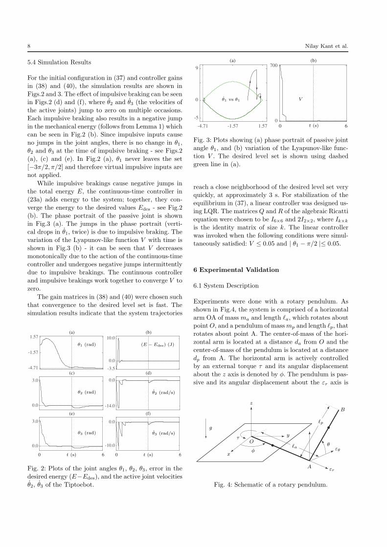
Experiments were done with a rotary pendulum. As

shown in Fig.4, the system is comprised of a horizontal

arm OA of mass ma and length ℓa, which rotates aboutpointO, and a pendulum of massmp and length ℓp, that

rotates about point A. The center-of-mass of the hori-

zontal arm is located at a distance da from O and the

center-of-mass of the pendulum is located at a distance

dp from A. The horizontal arm is actively controlledby an external torque τ and its angular displacement

about the z axis is denoted by φ. The pendulum is pas-

sive and its angular displacement about the εr axis is

x

y

z

O

A

B

εθ

εr

φ

τ

ℓa

ℓp

θ

g

Fig. 4: Schematic of a rotary pendulum.

Stabilization of Energy Level Sets of Underactuated Mechanical Systems Exploiting Impulsive Braking 9

denoted by θ. The accleration due to gravity is denoted

by g. With the following definition:

[q1 q2]T = [φ θ]T (41)

the dynamics of the system can be expressed in the

from given by (7), where u = τ , and

M11 = γ1 + γ2 cos2 θ, M12 = γ3 sin θ, M22 = γ2

h1 = γ3 cos θ θ2 − φ θγ2 sin 2θ,

h2 = γ2 φ2 sin θ cos θ + γ4 cos θ

γ1 , mad2a +mp ℓ

2a, γ2 , mpd

2p

γ3 , −mp ℓadp, γ4 , mpgdp

(42)

The physical parameters of the experimental setup are

γ1 = 0.0120, γ2 = 0.0042, γ3 = −0.0038, γ4 = 0.1190

(43)

The control torque was applied by a 24-Volt perma-

nent magnet brushed DC motor5.The motor is driven

by a power amplifier6 operating in current mode. Themotor torque constant is 37.7 mNm/A and the am-

plifier gain is 4.4 A/volt. An electromagnetic friction

brake7 was integrated to the shaft of the DC motor.

In the OFF state, the brake engages a friction pad to

the shaft of the motor which prevents the shaft fromturning; in the ON state, the brake is disengaged and

the motor shaft rotates freely. For impulsive braking,

the brake was kept engaged till the active velocity φ

reached a close neighborhood of zero. The brake waspowered ON/OFF by sending command voltage signals

through an n-channel mosfet. The rotary pendulum was

interfaced with a dSpace DS1104 board and the Mat-

lab/Simulink environment was used for real-time data

acquisition and control with a sampling rate of 1 Khz.The angular positions of the links were measured us-

ing incremental optical encoders; the angular velocities

were obtained by differentiating and low-pass filtering

the position signals.

5 The motor manufacturer is Faulhaber Drive Systems. Themotor has a gearbox with a reduction ratio of 3.71 : 1.6 The amplifier is a product of Advanced Motion Control.7 The electromagnetic brake is manufactured by Anaheim

Automation, model BRK-20H-480-024. The brake can with-hold torques up to 3.4 Nm.

6.2 Selection of Controller Gains

The total energy of the system is obtained from (2) as

follows

E =1

2(γ1+γ2 cos

2 θ) φ2 +1

2γ2 θ

2 + γ3 sin θ φ θ + F

F = γ4 sin θ

(44)

For the control objective in (1), we choose Edes to be

equal to the energy associated with the homoclinic orbit

that contains the upright equilibrium[

φθ φ θ]

=[

0π/200]

or[

0−3π/200]

Using (44), the energy associated with the homoclinic

orbit can be written as

Edes = γ4 (45)

The passive joint of the rotary pendulum is revolute

and thus assumption 1 holds good. From the expres-

sions in (42) and (44), it can be verified that assump-tion 2 holds good. Similar to the Tiptoebot, we can

show that assumption 3 holds good. From (44) we know

that F is only a function of θ and therefore condi-

tion (ii) is trivially satisfied resulting in the solution

φ∗ = 0. In the compact set [−3π/2, π/2], the possiblesolutions of θ∗ obtained from condition (ii) are θ∗ =

{−3π/2,−π/2, π/2}. At θ∗ = π/2 or θ∗ = −3π/2 and

φ∗ = 0, E = Edes. Using condition (iii), we therefore

get θ∗ = −π/2; this implies that Ke should be chosento satisfy

V (t = 0) < 2Keγ24 (46)

At the lower equilibrium configuration where [φ θ φ θ] =

[0 −π/2 0 0], we have V = 2Keγ24 . This violates the in-

equality in (46). This implies that our controller cannot

swing-up the pendulum when the system is exactly at

the lower equilibrium.Therefore, in experiments, a small

external perturbation was provided such that the sys-

tem is not at the lower equilibrium at the initial time.For the experimental results presented herein, the ini-

tial configuration of the system after the perturbation

was measured as[

φ(0) θ(0) φ(0) θ(0)]T

=[

0.01−1.420.050]T

(47)

For the initial conditions in (47) and physical parameter

values in (43), the following gains satisfied conditions

(i)-(iii):

Kp = 0.5, Kc = 0.08, Kd = 0.3, Ke = 100 (48)

For the above set of gains, the experimental results are

presented next.

10 Nilay Kant et al.

6.3 Experimental Results

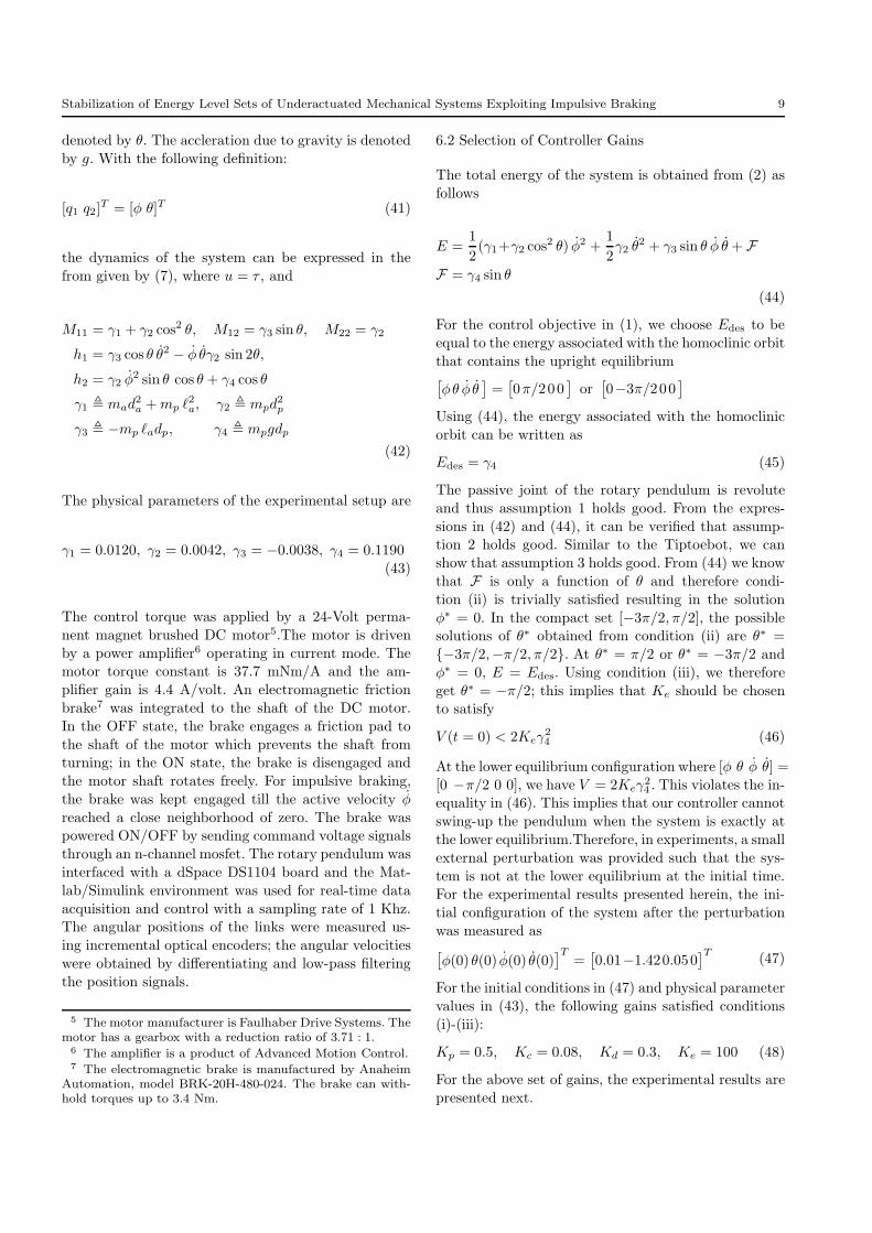
The experimental results are shown in Fig.5. The con-

troller for level set stabilization was active for the first

20 s. At the end of this period, the system trajectories

reached a close neighborhood of the upright equilibrium[φ θ φ θ] = [0 −3π/2 0 0] and the following linear con-

troller was invoked for stabilization:

τs = 1.4φ− 20.23(θ + 3π/2) + 1.14φ− 1.98θ

The poles of the closed-loop system were located at−37.0± 20.0 i and −1.0± 1.2 i.

The pulses shown on the top of Figs.5 (e) and (f)

correspond to the time intervals when the brake was en-

gaged (OFF) during level set stabilization. The brakewas disengaged (ON) when the condition | φ |≤ µ was

satisfied; the value of µ was chosen to be small, equal to

0.1 rad/s. The time intervals required for braking were

very short (≈ 0.04 s, on average); this implies that thebrakings were impulsive in nature. The effect of impul-

sive braking can be seen in Fig.5 (b) where φ jumps

to almost zero value upon engagement of the brake on

multiple occasions. It can be seen from Fig.5 (c) that

the amplitude of the pendulum gradually increases andfinally reaches a close neighborhood of the upright equi-

librium configuration. The derivative of the Lyapunov-

like function is shown in Fig.5 (f). It can be seen that

-4.71

1.57

-1.5

1.5

0 35 0 35

-1.0

0.0

1.01.0

-0.3

0.3

-15

0

(a) (b)

(c) (d)

(e) (f)

0.0

-1.0

-1.57 0.0

t (s)t (s)

φ (rad)

θ (rad)

φ (rad/s)

θ (rad/s)

τ (Nm) V

Fig. 5: Rotary pendulum experimental results: (a)-(d)

are plots of joint angles and joint velocities, (e) control

torque, and (f) derivative of Lyapunov-like function.The brake pulses are shown within plots (e) and (f),

the peaks represent time intervals when the brakes were

engaged.

-4.71

1.57

-7.0

7.0

0 20 0 20

-0.5

0.0

0.5 2.0

0.0

-2.0

-1.57 0.0

t (s)t (s)

φ (rad)

θ (rad)

φ (rad/s)

θ (rad/s)

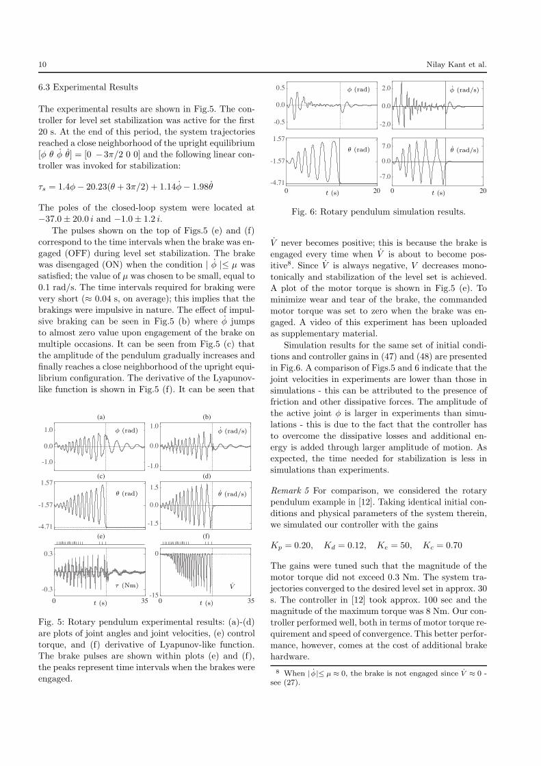
Fig. 6: Rotary pendulum simulation results.

V never becomes positive; this is because the brake is

engaged every time when V is about to become pos-

itive8. Since V is always negative, V decreases mono-

tonically and stabilization of the level set is achieved.A plot of the motor torque is shown in Fig.5 (e). To

minimize wear and tear of the brake, the commanded

motor torque was set to zero when the brake was en-

gaged. A video of this experiment has been uploadedas supplementary material.

Simulation results for the same set of initial condi-tions and controller gains in (47) and (48) are presented

in Fig.6. A comparison of Figs.5 and 6 indicate that the

joint velocities in experiments are lower than those in

simulations - this can be attributed to the presence offriction and other dissipative forces. The amplitude of

the active joint φ is larger in experiments than simu-

lations - this is due to the fact that the controller has

to overcome the dissipative losses and additional en-

ergy is added through larger amplitude of motion. Asexpected, the time needed for stabilization is less in

simulations than experiments.

Remark 5 For comparison, we considered the rotary

pendulum example in [12]. Taking identical initial con-

ditions and physical parameters of the system therein,we simulated our controller with the gains

Kp = 0.20, Kd = 0.12, Ke = 50, Kc = 0.70

The gains were tuned such that the magnitude of the

motor torque did not exceed 0.3 Nm. The system tra-

jectories converged to the desired level set in approx. 30

s. The controller in [12] took approx. 100 sec and themagnitude of the maximum torque was 8 Nm. Our con-

troller performed well, both in terms of motor torque re-

quirement and speed of convergence. This better perfor-

mance, however, comes at the cost of additional brake

hardware.

8 When | φ |≤ µ ≈ 0, the brake is not engaged since V ≈ 0 -see (27).

Stabilization of Energy Level Sets of Underactuated Mechanical Systems Exploiting Impulsive Braking 11

7 Conclusion

A control strategy was presented for stabilization of en-

ergy level sets of underactuated systems with one pas-

sive DOF. The level set is defined with the help of a

Lyapunov-like function that has been commonly used

in the literature. Unlike existing energy-based methods,that have relied on continuous control inputs alone, our

control strategy uses continuous control inputs and in-

termittent impulsive brakings. The continuous control

is designed to make the time derivative of the Lyapunov-like function negative semi-definite. When this condi-

tion cannot be enforced, the impulsive inputs are in-

voked. This results in negative jumps in the Lyapunov-

like function and guarantees its negative semi-definiteness

under continuous control for some finite time interval.Thus, a combination of continuous and impulsive in-

puts guarantees monotonic convergence of the system

trajectories to the desired energy level set, which can

be periodic, or non-periodic as in the case of homoclinicorbits, depending on the choice of desired energy. More

importantly, it allows us to develop a general frame-

work for energy-based orbital stabilization, which is an

important contribution of this paper. A set of condi-

tions, that impose constraints on the choice of con-troller gains, have to be satisfied for applicability of

the control strategy. These conditions are easily sat-

isfied by systems commonly studied in the literature

such as the pendubot, acrobot, inertia-wheel pendu-lum, and pendulum on a cart. In this paper, the control

strategy was demonstrated in a three-DOF underactu-

ated system using simulations and the two-DOF rotary

pendulum using experiments. In experiments, impulsive

brakings were not applied by the motor; instead, theywere applied by a friction brake mounted co-axially

with the motor shaft. This requires additional hard-

ware but there are two important advantages of using

the brake. In physical systems, impulsive inputs are im-plemented using high-gain feedback, which can result in

actuator saturation. Since our impulsive control strat-

egy requires the active velocities to be reduced to zero,

a brake is a natural choice and it eliminates the pos-

sibility of motor torque saturation. The advantage ofusing a brake is also manifested in the time required

for stabilization. A comparison of our approach with

an approach in the literature shows significant reduc-

tion in the time for convergence for the same set of ini-tial conditions. Our future work will focus on extension

of our approach to orbital stabilization using virtual

holonomic constraints.

8 Appendix

8.1 Proof of Lemma 1

The proof of Lemma 1 is provided here for the gen-

eral case where the underactuated system has m pas-sive and n−m active generalized coordinates, i.e. q1 ∈

Rn−m, q2 ∈ Rm and u ∈ Rn−m. The equation of mo-

tion has the form in (7) with M11 ∈ R(n−m)×(n−m),

M22 ∈ Rm×m, h1 ∈ R(n−m), and h2 ∈ Rm. The changein the energy due to application of an impulsive input

is equal to the change in the kinetic energy:

∆E =1

2q+

T

M(q)q+ −1

2q−

T

M(q)q−

=1

2

[

q+T

1 M11 q+1 − q−

T

1 M11 q−

1

]

+1

2

[

q+T

2 M22 q+2 − q−

T

2 M22 q−

2

]

+ q+T

1 M12 q+2 − q−

T

1 M12 q−

2 (A.1)

The impulse manifold, given in (12) for m ≥ 1, is

q+2 = q−2 −M−122 MT

12(q+1 − q−1 ) (A.2)

Substitution of q+2 from (A.2) into (A.1) yields

∆E =1

2

[

q+T

1 M11 q+1 − q−

T

1 M11 q−

1

]

+1

2

[

q−2 −M−122 MT

12(q+1 − q−1 )

]TM22×

[

q−2 −M−122 MT

12(q+1 − q−1 )

]

−1

2q−

T

2 M22 q−

2 − q−T

1 M12 q−

2

+ q+T

1 M12

[

q−2 −M−122 MT

12(q+1 − q−1 )

]

Expanding, canceling, and regrouping the terms on the

right-hand side of the above equation yields

∆E =1

2q+

T

1

[

M11 −M12M−122 MT

12

]

q+1

−1

2q−

T

1

[

M11 −M12M−122 MT

12

]

q−1 (A.3)

Similar to (10), B(q) is defined for the general case as

follows

B(q) =[

M11 −M12M−122 MT

12

]−1(A.4)

From the properties of the mass matrix M(q), it can beshown that B(q) is well-defined; also, it is symmetric

and positive-definite, i.e., B(q) = BT (q) > 0. Substitu-

tion of (A.4) into (A.3) gives (13).

12 Nilay Kant et al.

8.2 Proof of Lemma 2

Impulsive inputs result in no change in the generalized

coordinates. Additionally, impulsive braking results in

q+1 = 0. Therefore, from the definition of V in (15), ∆V

for impulsive braking can be expressed as

∆V =1

2

[

Ke(E+− Edes)

2 −Ke(E−− Edes)

2

−q−T

1 Kd q−

1

]

=1

2

[

Ke(E++ E−− 2Edes)∆E − q−

T

1 Kd q−

1

]

=1

2

[

Ke(2E+−∆E − 2Edes)∆E − q−

T

1 Kd q−

1

]

where ∆E is defined in (13). Substitution of ∆E from

(14) in the equation above yields

∆V = −1

2

[

(q−T

1 B−1q−1 )Ke{E+− Edes +

1

4q−

T

1 B−1q−1 }

+ q−T

1 Kd q−

1

]

= −1

2q−

T

1

[

Ke{E+− Edes +

1

4q−

T

1 B−1q−1 }B−1

+Kd

]

q−1

= −1

2q−

T

1

[

1

4

{

Ke q−

T

1 B−1 q−1

}

B−1

+Kd +Ke(E+ − Edes)B

−1

]

q−1

which is the same as in (16). Since B, defined in (A.4), is

positive-definite, {Ke q−

T

1 B−1 q−1 }B−1 is positive-definite.

Therefore, if[

Kd +Ke(E+ − Edes)B

−1(q)]

is positive-definite, ∆V ≤ 0 and ∆V = 0 iff q−1 = 0.

8.3 Assumption 3 holds for Tiptoebot

A constant value of u implies τ2 and τ3 are constants.

A constant value of q1 implies θ2 = θ3 = 0 from (32).

Substituting these conditions in (7), (8) and (2), we get

M12 q2 + M12 q2 −1

2

[

∂M22

∂q1

]T

q22 +

[

∂F

∂q1

]T

= u

M22 q2 + M22 q2 −1

2

[

∂M22

∂q2

]

q22 +∂F

∂q2= 0

E =1

2M22q

22 + F

(A.5)

From (33), it can be seen that M12 and M22 are only

function of q1, which is constant. Therefore, in (A.5)M12 = M22 = 0; also, (∂M22/∂q2) = 0 since M22 is

not a function of q1. Furthermore, from the passivity

property of underactuated mechanical systems [32,35],

we have E = uT q1 = 0. This implies E is constant in

(A.5). Manipulating (A.5) to eliminate q2 and q2, we

get

[

∂F

∂q1

]T

−M12

M22

∂F

∂q2−

(E −F)

M22

[

∂M22

∂q1

]T

= u (A.6)

From (33), it can be seen that M12 and M22 are func-

tions of q1 only; therefore, M12, M22, and (∂M22/∂q1)T

are constants. Furthermore u and E are constants andF is a function of q2 since q1 is constant. Therefore

(A.6) can be manipulated and written in the form

sin[q2 + c1] = c2 (A.7)

where c1 and c2 are constants. This implies that q2 is

constant.

Acknowledgements

The authors gratefully acknowledge the support pro-

vided by the National Science Foundation, NSF Grant

CMMI-1462118.

Data Availability

The datasets generated during and/or analysed during

the current study are available from the corresponding

author on reasonable request.

Conflict of Interest

The authors declare that they do not have any conflict

of interest.

References

1. F. Plestan, J. W. Grizzle, E. R. Westervelt, and G. Abba,“Stable walking of a 7-dof biped robot,” IEEE Transac-

tions on Robotics and Automation, vol. 19, no. 4, pp. 653–668, 2003.

2. E. R. Westervelt, C. Chevallereau, J. H. Choi, B. Morris,and J. W. Grizzle, Feedback Control of Dynamic Bipedal

Robot Locomotion. CRC press, 2007.3. M. Maggiore and L. Consolini, “Virtual holonomic con-

straints for Euler- Lagrange systems,” IEEE Transactions

on Automatic Control, vol. 58, no. 4, pp. 1001–1008, 2013.4. A. Shiriaev, J. W. Perram, and C. Canudas-de Wit,

“Constructive tool for orbital stabilization of underac-tuated nonlinear systems: Virtual constraints approach,”IEEE Transactions on Automatic Control, vol. 50, no. 8,pp. 1164–1176, 2005.

5. A. Mohammadi, M. Maggiore, and L. Consolini, “Dy-namic virtual holonomic constraints for stabilization ofclosed orbits in underactuated mechanical systems,” Au-

tomatica, vol. 94, pp. 112–124, 2018.

Stabilization of Energy Level Sets of Underactuated Mechanical Systems Exploiting Impulsive Braking 13

6. N. Kant and R. Mukherjee, “Orbital stabilization of un-deractuated systems using virtual holonomic constraintsand impulse controlled Poincare maps,” Systems & Con-

trol Letters, vol. 146, p. 104813, 2020.7. I. Fantoni, R. Lozano, and M. Spong, “Energy based con-

trol of the pendubot,” IEEE Trans. on Automatic Control,vol. 45, no. 4, pp. 725–729, 2000.

8. X. Xin and T. Yamasaki, “Energy-based swing-up con-trol for a remotely driven acrobot: Theoretical and exper-imental results,” IEEE Transactions on Control Systems

Technology, vol. 20, no. 4, pp. 1048–1056, 2012.9. I. Fantoni, R. Lozano, and M. Spong, “Stabilization of

the reaction wheel pendulum using an energy approach,”in European Control Conference, 2001, pp. 2552–2557.

10. R. Lozano, I. Fantoni, and D. J. Block, “Stabilizationof the inverted pendulum around its homoclinic orbit,”Systems & Control Letters, pp. 197–204, 2000.

11. H. Oka, Y. Maruki, H. Suemitsu, and T. Matsuo, “Non-linear control for rotational movement of cart-pendulumsystem using homoclinic orbit,” International Journal of

Control, Automation and Systems, vol. 14, no. 5, pp. 1270–1279, 2016.

12. I. Fantoni and R. Lozano, “Stabilization of the Furutapendulum around its homoclinic orbit,” International

Journal of Control, vol. 75, no. 6, pp. 390–398, 2002.13. X. Xin and M. Kaneda, “Swing-up control for a 3-dof

gymnastic robot with passive first joint: design and anal-ysis,” IEEE Transactions on Robotics, vol. 23, no. 6, pp.1277–1285, 2007.

14. T. Albahkali, R. Mukherjee, and T. Das, “Swing-up con-trol of the pendubot: An impulse-momentum approach,”IEEE Transactions on Robotics, vol. 25, no. 4, pp. 975–982,2009.

15. B. Brogliato, S. . Niculescu, and P. Orhant, “On the con-trol of finite-dimensional mechanical systems with unilat-eral constraints,” IEEE Transactions on Automatic Con-

trol, vol. 42, no. 2, pp. 200–215, Feb 1997.16. W. M. Haddad, V. Chellaboina, and S. G. Nersesov, Im-

pulsive and Hybrid Dynamical Systems. Princeton Seriesin Applied Mathematics, 2006.

17. R. I. Leine and N. Van de Wouw, Stability and Conver-

gence of Mechanical Systems with Unilateral Constraints.Springer Science & Business Media, 2007, vol. 36.

18. N. Van De Wouw and R. Leine, “Robust impulsive con-trol of motion systems with uncertain friction,” Interna-

tional Journal of Robust and Nonlinear Control, vol. 22,no. 4, pp. 369–397, 2012.

19. D. D. Bainov and P. S. Simeonov, Systems with Impulse

Effect: Stability, Theory, and Applications. Ellis Horwood,1989.

20. B. M. Miller and E. Y. Rubinovich, Impulsive Control in

Continuous and Discrete-Continuous Systems. SpringerScience & Business Media, 2012.

21. R. Goebel, R. G. Sanfelice, and A. R. Teel, Hybrid Dynam-

ical Systems: Modeling Stability, and Robustness. Prince-ton University Press, Princeton, NJ, 2012.

22. F. B. Mathis, R. Jafari, and R. Mukherjee, “Impulsive ac-tuation in robot manipulators: Experimental verificationof pendubot swing-up,” IEEE Transactions on Mechatron-

ics, vol. 19, no. 4, pp. 1469–1474, 2014.23. R. Jafari, F. B. Mathis, R. Mukherjee, and H. Khalil,

“Enlarging the region of attraction of equilibria of under-actuated systems using impulsive inputs,” IEEE Trans-

actions on Control Systems Technology, vol. 24, no. 1, pp.334–340, 2016.

24. N. Kant, R. Mukherjee, D. Chowdhury, and H. K. Khalil,“Estimation of the region of attraction of underactuatedsystems and its enlargement using impulsive inputs,”IEEE Transactions on Robotics, vol. 35, no. 3, pp. 618–632, June 2019.

25. N. Kant and R. Mukherjee, “Impulsive dynamics andcontrol of the inertia-wheel pendulum,” IEEE Robotics

and Automation Letters, vol. 3, no. 4, pp. 3208–3215, 2018.26. N. Kant, R. Mukherjee, and H. K. Khalil, “Swing-up of

the inertia wheel pendulum using impulsive torques,” inProc. IEEE Conference on Decision and Control, 2017, pp.5833–5838.

27. N. Kant, R. Mukherjee, and H. K. Khalil, “Stabilizationof homoclinic orbits of two degree-of-freedom underactu-ated systems,” in 2019 American Control Conference, July2019, pp. 699–704.

28. N. Kant and R. Mukherjee, “Non-prehensile manipula-tion of a devil-stick: planar symmetric juggling using im-pulsive forces,” Nonlinear Dynamics, vol. 103, no. 3, pp.2409–2420, 2021.

29. Y. Li, C. Li, Z. He, and Z. Shen, “Estimating and enlarg-ing the region of attraction of multi-equilibrium pointssystem by state-dependent edge impulses,” Nonlinear Dy-

namics, vol. 103, no. 3, pp. 2421–2436, 2021.30. B. Brogliato, R. Lozano, B. Maschke, and O. Egeland,

Dissipative Systems Analysis and Control. Springer, 2020.31. L. L. Flynn, R. Jafari, and R. Mukherjee, “Active

synthetic-wheel biped with torso,” IEEE Transactions on

Robotics, vol. 26, no. 5, pp. 816–826, 2010.32. D. Liu, W. Guo, J. Yi, and D. Zhao, “Passivity-based-

control for a class of underactuated mechanical systems,”in IEEE International Conference on Intelligent Mechatron-

ics and Automation, 2004, pp. 50–54.33. B. Brogliato, Nonsmooth Mechanics. Models, Dynamics

and Control. Springer Nature Switzerland AG, 2020.34. N. Kant, “Exploiting impulsive inputs for stabilization

of underactuated robotic systems: Theory and experi-ments,” Ph.D. dissertation, Michigan State University,2020.

35. R. Ortega, J. A. L. Perez, P. J. Nicklasson, and H. J. Sira-Ramirez, Passivity-based control of Euler-Lagrange systems:

Mechanical, Electrical and Electromechanical Applications.Springer Science & Business Media, 2013.

Figures

Figure 1

The three-link underactuated tiptoebot has two active joints and one passive joint.

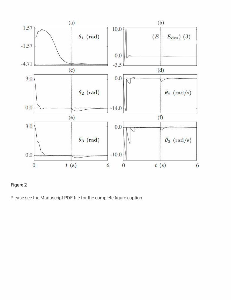
Figure 2

Please see the Manuscript PDF �le for the complete �gure caption

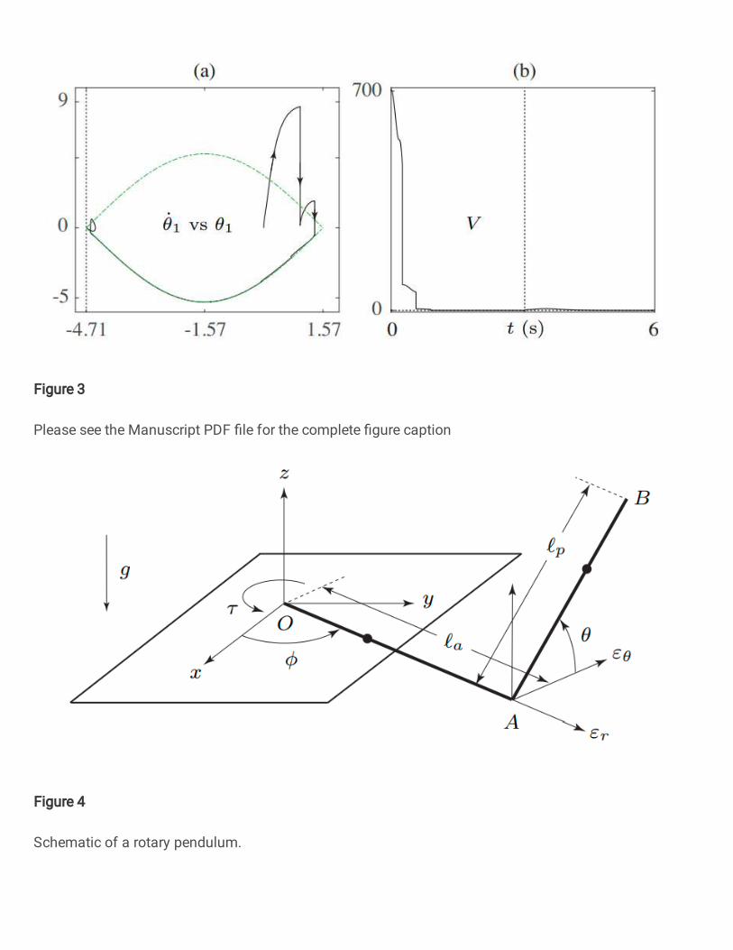
Figure 3

Please see the Manuscript PDF �le for the complete �gure caption

Figure 4

Schematic of a rotary pendulum.

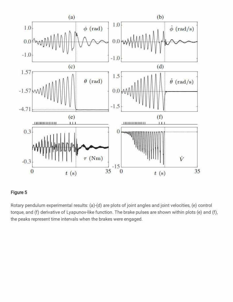
Figure 5

Rotary pendulum experimental results: (a)-(d) are plots of joint angles and joint velocities, (e) controltorque, and (f) derivative of Lyapunov-like function. The brake pulses are shown within plots (e) and (f),the peaks represent time intervals when the brakes were engaged.

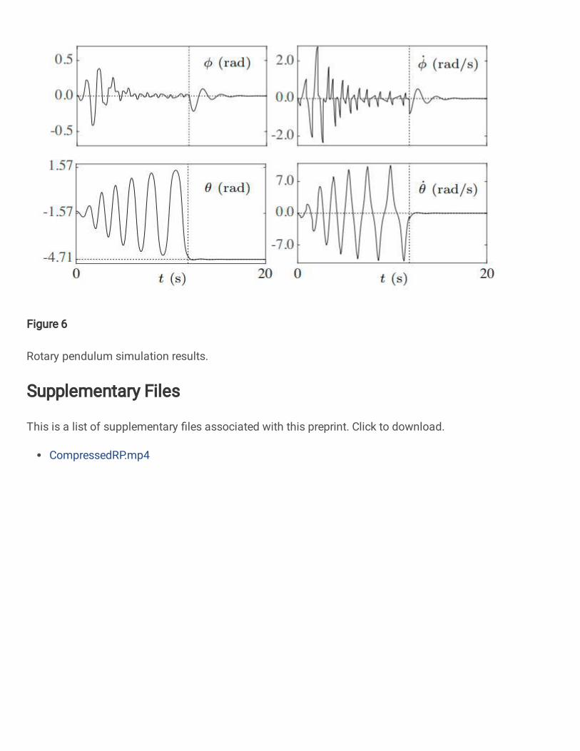
Figure 6

Rotary pendulum simulation results.

Supplementary Files

This is a list of supplementary �les associated with this preprint. Click to download.

CompressedRP.mp4