Stability of Age Dependent Hawkes Processes

Stability of Age Dependent HawkesProcesses

Ph.D. Thesis by

Mads Bonde [email protected]

Department of Mathematical SciencesUniversity of CopenhagenSubmitted August 2019

Mads Bonde RaadDepartment of Mathematical SciencesUniversity of CopenhagenUniversitetsparken 5, 2100 CopenhagenDenmark

Supervisors: Prof. Susanne DitlevsenUniversity of Copenhagen, Denmark

Prof. Eva LocherbachUniversite Paris 1, France

Assessment Committee: Prof. Thomas Mikosch (chair)University of Copenhagen, Denmark

Prof. Carl Graham

Ecole Polytechnique, France

Prof. Jesper MøllerAalborg university, Denmark

ISBN: 978-87-7078-894-6

Contents

1 Preface 51.1 Abstract . . . . . . . . . . . . . . . . . . . . . . . . . . . . 51.2 Dansk Resume . . . . . . . . . . . . . . . . . . . . . . . . 61.3 Acknowledgements . . . . . . . . . . . . . . . . . . . . . . 71.4 A Short Introduction . . . . . . . . . . . . . . . . . . . . . 81.5 Thesis Structure . . . . . . . . . . . . . . . . . . . . . . . . 11

2 Notation and Prerequisities 122.1 Probability Theory on Measures . . . . . . . . . . . . . . . 13

2.1.1 Measure Theory Spaces of Measures . . . . . . . . . 132.1.2 Random Measures . . . . . . . . . . . . . . . . . . 152.1.3 Poisson Random Measure . . . . . . . . . . . . . . 16

2.2 Core Assumptions and Definitions . . . . . . . . . . . . . . 212.3 Age Dependent Hawkes Process . . . . . . . . . . . . . . . 222.4 Linear Hawkes Process . . . . . . . . . . . . . . . . . . . . 262.5 Markovian Hawkes Processes . . . . . . . . . . . . . . . . . 302.6 A Brief Overview of Hawkes Process Results . . . . . . . . 31

3 A Multiclass Hawkes Process Stabilized by Inhibition 353.1 Introduction . . . . . . . . . . . . . . . . . . . . . . . . . . 353.2 Setup For This Chapter . . . . . . . . . . . . . . . . . . . 353.3 Proof of Theorem 3.2.1 . . . . . . . . . . . . . . . . . . . . 393.4 Discussion And Further Research Topics . . . . . . . . . . 44

4 Stability for ADHP’s With a Refractory Period 484.1 Introduction . . . . . . . . . . . . . . . . . . . . . . . . . . 484.2 Setup For This Chapter . . . . . . . . . . . . . . . . . . . 494.3 Main Result . . . . . . . . . . . . . . . . . . . . . . . . . . 524.4 Proof of Main Result . . . . . . . . . . . . . . . . . . . . . 53

Contents

4.5 Age Dependent Hawkes Processes With Erlang Weight Func-tions . . . . . . . . . . . . . . . . . . . . . . . . . . . . . . 69

5 Renewal Time Points For Hawkes Processes 735.1 Introduction, Purpose, and Results . . . . . . . . . . . . . 735.2 Setup In This Chapter . . . . . . . . . . . . . . . . . . . . 745.3 Constructing a Renewal Time Point for a Hawkes Process . 805.4 Hawkes Processes In a Markov Chain Framework . . . . . 855.5 Applications . . . . . . . . . . . . . . . . . . . . . . . . . . 87

5.5.1 Bound On The Coupling Time . . . . . . . . . . . . 875.5.2 Asymptotics . . . . . . . . . . . . . . . . . . . . . . 88

5.6 Discussion and Outlook . . . . . . . . . . . . . . . . . . . 915.7 Proofs . . . . . . . . . . . . . . . . . . . . . . . . . . . . . 92

5.7.1 Proofs of Section 2 Results . . . . . . . . . . . . . . 925.7.2 Proofs of Section 3.1 Results . . . . . . . . . . . . . 935.7.3 Proofs of Section 3.2 Results . . . . . . . . . . . . . 105

6 Mean-field Limit and Propagation of Chaos 1076.1 Setup in This Chapter . . . . . . . . . . . . . . . . . . . . 1086.2 The Limit System . . . . . . . . . . . . . . . . . . . . . . . 1096.3 Large Network Asymptotics and Weight Approximations . 1116.4 The Mean-Field Limit In the Case of a Hard Refractory

Period . . . . . . . . . . . . . . . . . . . . . . . . . . . . . 1136.5 Proofs of Section 6 Results . . . . . . . . . . . . . . . . . . 118

7 Appendix 1277.1 Point Process Results . . . . . . . . . . . . . . . . . . . . . 1277.2 Analysis results . . . . . . . . . . . . . . . . . . . . . . . . 1277.3 Splitting Two PRMs . . . . . . . . . . . . . . . . . . . . . 1287.4 The Random Exchange Process . . . . . . . . . . . . . . . 132

4

Chapter 1

Preface

1.1 Abstract

The primary subject of this dissertation is Hawkes processes with a focuson stability and with neuroscience as a primary application. The Hawkesprocess has received much attention in the last decade for modeling eventsthat exhibit self excitation - or inhibition. There are many examples ofphenomena of interest which exhibit such behavior, including finance thatpropagate through a market giving rise to volatility clustering observations[2], interactions on social media [42], and pattern dependencies in DNA[39].

Hawkes processes are point processes where the intensity function isstochastic and allowed to depend on the past history, introducing memoryin the temporal evolution of the stochastic process. We work with anextension to the ordinary Hawkes model called an age dependent Hawkesprocess, where the intensity of a unit may also depend on the time sinceits last jump.

The classical results concerning stability for Hawkes processes found in[5] assume bounds on the strength of the functional connectivity betweenunits in the system. However, by taking inhibition into account, we willbe able to produce new stability results for Hawkes processes. We shallalso discuss stability for Hawkes processes from a regeneration point ofview. We will give a constructive proof of a random time such that theincremented Hawkes process is a Hawkes process in itself independent ofthe past. Standard Markov chain techniques allow us to prove variousasymptotic results for the Hawkes process. Finally, we end by studyingthe mean-field limit of age dependent Hawkes processes.

1 Preface

1.2 Dansk Resume

Denne afhandling beskæftiger sig med Hawkes-processer med særligt fokuspa stabilitet. Det primært tiltænkte anvendelsesomrade for afhandlingensresultater er neuroscience. Det sidste arti har Hawkes-processer faet megetvidenskabelig opmærksomhed som model til at beskrive fænomener, hvorider indgar selv-excitering eller -inhibering. Finansielle kriser [2], inter-aktion pa sociale medier [42] og DNA mønstre [39] er alle eksempler pafænomener med en sadan adfærd.

Hawkes-processer er punktprocesser, hvor intensiteten er stokastisk ogafhænger af fortiden. I denne afhandling arbejder vi med en udviddelseaf den ordinære Hawkes-proces, hvor intensiteten ogsa ma afhænge aftiden siden sidste spring. Denne udvidede klasse af processer kalder viAlders-afhængige Hawkes-processer.

De klassiske resultater om stabilitet af Hawkes-processer, først beskreveti [5], antager, at den exiterende eller inhiberende styrke pa tværs af en-heder i netværket er begrænset. Ved at benytte inhiberingen i systemeter det muligt for os at formulere nye resultater for stabilitet af Hawkes-processer.

Deruover diskuteres regeneration af Hawkes-processer. Vi konstruereren stokastisk tid, saledes at Hawkes-processen i tiden derefter er uafhængigaf fortiden. Dette muliggør benyttelse af standard Markov-kæde-teknikkertil at vise asymptotiske resultater for Hawkes-processer. Endeligt præsen-terer vi mean-field-resultater for Alders-afhængige Hawkes-processer

6

1.3 Acknowledgements

1.3 Acknowledgements

I want to express my deep gratitude to my principal supervisor SusanneDitlevsen for granting me the chance to become a Ph.D. student underher supervision, and I want to thank her for the supervision and guid-ance through these three years. I also want to thank my co-supervisorEva Locherbach, for the great supervision and for her tireless efforts inreading, correcting and improving my work. Furthermore, I thank herfor the opportunity of working with her in Paris for a year. Most ofmy research is based on probability theory and stochastic processes. Myknowledge of these topics has been founded by teachings and materialsfrom UCPH. I learned Markov process theory from Anders Rønn Nielsen,stochastic process theory from Alexander Sokol and Measure theory fromErnst Hansen. I thank them and my other teachers throughout my stud-ies. During my eight years studying and researching math I have beengrateful for my friend and now colleague Martin, who has always beenavailable for coffee and math discussions about Null-set problems. I’vehad the pleasure of sharing office with many great colleagues. I small-talkmore than each of them, maybe more than ’em all combined. I thank allof them for enduring that, and for the fun and interesting time at the of-fice. My deep and sincere gratitude goes to Anna Laksafoss for helping metyping this thesis, and making it readable. I could not have completedthis dissertation without support from my family and my special one.They have been very supportiveand shown me much patience. Ithank them, and ask for forgive-ness for the many times that I havepaid attention to a math thoughtinstead of the reality. I have twobirds of the species Agapornis Per-sonata named Hanne and Eddie.They have not been supportive, norhave they have they shown any pa-tience.I thank them anyways.

7

1 Preface

1.4 A Short Introduction

The age dependent Hawkes process (ADHP) is a class of processes in-cluding the well known nonlinear Hawkes process. A Hawkes process Zis defined by its conditional intensity. This object may be described in aless formal way byλt = P (Z jumps in [t, t+ dt) | Ft) . The defining property for a Hawkesprocess is that its intensity is a function of the aggregating integral∫ t−

0 h (t− s) dZs for some fixed weight function h. The extension whichdefines the ADHP is that the intensity is allowed to also depend on theage of Z, which is the process measuring the time passed since the lastjump of Z. This makes it possible to directly model individual refrac-tory periods in a system, such as neural networks on an individual level.The Hawkes process may be extended to an N -dimensional version in anatural way: The i’th unit has a conditional intensity that depends on asum of aggregating integrals

∑Nj=1

∫ t0 hij (t− s) dZj

s . Often it is assumedthat the relation between the integral and the intensity of the i’th unitis Li-Lipschitz. In this case, a classic result from [5] states that a one-dimensional Hawkes process is stable if L ‖h‖L1 < 1. A similar resultexists for the multivariate process. An introduction to ADHPs are givenin chapter 2, along with natural prerequisites such as the underlying mea-sure theory.

The first result, presented in chapter 3, treats a specific submodelof ordinary multivariate Hawkes processes. The aim is to show that forHawkes processes where inhibition is present, stability is not necessarilydue to limited connectivity strength. Balance between exciting and in-hibiting effects can also induce stability in the system. In the describedmodel, the units in the network are divided into two homogeneous popu-lations. One population is exciting the system, while the other populationacts inhibiting on the system. Moreover, the specific choice of weight func-tions makes the memory processes Markovian, which allows us to studystability in the framework of Harris recurrence and invariant measuresfrom Markov process theory. The main result is proven using Foster-Lyapunov theory, and gives a stability criteria which does not imply, noris implied by, the classic stability results

The next result, presented in chapter 4, is about ADHPs with a re-

8

1.4 A Short Introduction

fractory period. That is, we impose a strong bound on the intensity in afixed window after each jump. Such behavior is seen in neurons, where thebiophysical process of inducing an electrical impulse (a so-called ”spike”)forbids it from repeating such an impulse in the following ≈ 2ms. We areable to obtain classic stability results without imposing a sub-criticalitybound on h. Indeed, there is a stationary and mixing version of theHawkes process, and other Hawkes processes with regular starting condi-tions converge in variation towards it. The proof relies on constructinga random measure defined on the entire real line with the same dynam-ics as a Hawkes process. This has been done by [5] in the case whereλ is bounded using Picard iteration. However, when including the agevariables, it is no longer clear that the Picard-iterates exist. Moreover, abound on the Picard-iteration is needed in order to obtain convergence.We use growth-bounds induced by the refractory period to produce a sta-tionary process dominating the Picard-iterates.

In chapter 5 we study stability of Hawkes processes from another per-spective, namely using regeneration. We study regeneration propertiesunder both the classic stability criteria and the ones in chapter 4. Wegive a constructive proof of a regeneration time ρ for a Hawkes process,satisfying that the increment process Zρ+ is independent of the past. Thiswork may be seen as an extension of the work done in [10] which treatsthe case where the weight function h is of bounded support. However, theproblem changes qualitatively when h is of unbounded support since theaggregating integral

∫ t0 h (t− s) dZs may never regenerate. Instead, we

utilize the driving Poisson random measure of the Hawkes process, whichenjoys temporal and spatial independence. Using the Poisson measure,we are able to construct a scheme similar in spirit to Nummelin splittingconstructions. Said in a colloquial way, we attempt to restart the Hawkesprocess at random (stopping) times. At each attempt, the independenceproperties of the Poisson measure allow us to flip a coin, deciding if theattempt is successful. The constructed regeneration time turns out to bea stopping time with respect to a filtration that is strictly larger thanthe filtration induced by Z. We also provide criteria for the existence ofmoments for the regeneration time. Finally, we use this to prove resultsabout the Hawkes process, such as various CLTs.

Finally, in chapter 6, we discuss mean-field limits in a multipopulation

9

1 Preface

framework, similar to what has been done in [13]. We consider a largeHawkes network and aim to take the N →∞ limit. We assume that thereis a fixed number of populations, and that all units within a populationare similar. We prove standard results such as propagation of chaos andasymptotic independence of a fixed finite subset of neurons.

10

1.5 Thesis Structure

1.5 Thesis Structure

The dissertation consists of the following:

• Chapter 2, section 1 gives an introduction to probability theory onmeasures, and is based on appendix material from [14] and [11].Section 2-6 gives an introduction to the Hawkes process.

• Chapter 3 presents a class of Hawkes processes for which we presentstability results. The material is based on ongoing work by Locherbachand Raad.

• Chapter 4 is essentially the first half of [14] by Raad et al. concern-ing stability of Age Dependent Hawkes processes. The material issubmitted for peer-review1.

• Chapter 5 is essentially the article [38] by Raad about regenerationfor Hawkes processes. The material is submitted for peer-review.

• Chapter 6 is essentially the second half of [14] by Raad et al. treatingmean-field limits for Hawkes processes. The material is submittedfor peer-review1.

• Chapter 7 is an appendix based on the appendices of the abovementioned articles.

1Update November 2019: The material is to appear in the journal AIHP (B)

11

Chapter 2

Notation andPrerequisities

We denote the set of real numbers as R and the subset of strictly posi-tive real numbers as R+. The set of strictly positive integers are denotedN and we define N0 := N ∪ 0, N := N ∪ ∞ . If v = (v1, . . . , vd) is

a d−dimensional Euclidian vector for some d ∈ N, then |v| =∑d

i=1 |vi|denotes the 1-distance. We introduce a background probability space(Ω,F , P ) and assume that this measure space is completed. If (Y,Y) isa measurable space then a measurable map X : Ω → Y is called a ran-dom variable taking values in Y . For a closed interval I unbounded tothe right, we denote a family of increasing σ-algebras (Ft)i∈I as a filtra-tion on the probabilty space. We shall always assume that a filtrationis satisfying the usual hypothesis meaning that for all t ∈ I P (A) = 0implies A ∈ Ft and

⋂s>tFs = Ft. Whenever a new filtration is defined,

it is implicitly assumed that we extend it to satisfy the usual conditions.A random variable X taking values in R is said to have q’th moment forsome q ≥ 0 if E |Xq| < ∞, and it is said to have exponential momentif E exp (cX) < ∞ for some c > 0. Likewise, we say that a functionf : R → R have q’th moment, respectively exponential moment, if∫xqf (x) dx < ∞, respectively

∫exp (cx) f (x) dx < ∞. We recall the

basic Stieltjes integration notation. Let g : R → R be a cadlag function.The variation of g on a bounded interval I is given by

Vg (I) = sup(xi)∈I

∑i

|g (xi)− g (xi−1)| <∞

2.1 Probability Theory on Measures

where I denotes the system of all finite sets of increasing indices (xi) ⊂ I.The function g is said to be of finite variation, if the variation is finiteon all bounded intervals. For such g there exists two singular σ−finitemeasures µ+

g , µ−g s.t. µg := µ+

g −µ−g which satisfies µg (a, b] = g (b)−g (a) .The variation measure |dg| := µ+

g + µ−g satisfies |dg| (a, b] = Vg (a, b]. If

f : R → R is a measurable function such that∫|f | |dµg| < ∞ then we

define the Lebesgue-Stieltjes integral as∫f (x) dg (x) =

∫f (x) dµg (x) ,

see e.g. [22] or [26]. If ν is a measure on R2 we shall abbreviate theintegral over a semi-closed box∫

1 (a, b] (x)1 (c, d] (y) f (x, y) dν (x, y) ,

as either∫ b

a

∫ d

c

f (x, y) dν (x, y) or

∫ b

a

∫ d

c

f (x, y) ν (dx, dy) .


2.1.1 Measure Theory Spaces of Measures

The purpose of this section is to provide a brief overview of measure the-ory on the space ME of boundedly finite measures defined on a c.s.m.s(Complete Separable Metric Space). Whenever a c.s.m.s. space (E, d) isintroduced, it is always assumed to be equipped with the topology andborel-algebra induced by its metric, unless otherwise written.

First, assume that (E, d) is merely a metric space. Let M 0E be the space

of totally finite measures on E, i.e. measures µ satisfying µ (E) <∞. Letus equip M 0 with a metric d0. For a set A ⊂ E let Aε be the superset ofA in E defined by all points with < ε d-distance to a point in A. Definethe map d0 : M 0

E ×M 0E → [0,∞) as

d0 (µ, ν) = inf ε > 0 µ (A) ≤ ν (Aε) + ε and ν (A) ≤ µ (Aε + ε) . (2.1)

13

2 Notation and Prerequisities

It may be verified that d0 is indeed a distance function, and it is charac-terized by weak convergence:

µnd0→ µ⇔ ∀f ∈ Cb (E) :

∫fdµn →

∫fdµ (2.2)

where Cb (E) denotes the set of continuous bounded E → R functions, see[11] Prop. A2.5II. Next, A measure ν on E is said to be boundedly finite ifDiam (A) <∞ implies that ν(A) <∞ for A ∈ BE. Let ME be the spaceof all boundedly-finite measures on (E,BE). Clearly M 0

E ⊂ME. We equipthis space with the metric of local d0 convergence in the standard way:Choose an arbitrary origin point o ∈ E. For a measure µ ∈ME and r ≥ 0denote µ(r) as the measure µ restricted to the ball Bd0 (o, r) . Define the

weak-hat metric d as

d (µ, ν) =

∫exp (−r)

d0(µ(r), ν(r)

)1 + d0

(µ(r), ν(r)

)dr. (2.3)

It may be seen that this topology is characterized by

µnd→ µ⇔:

∫fdµn →

∫fdµ ∀f ∈ Cb (E) with f ≡ 0 outside of a bounded set.

Assume now that E is a c.s.m.s. space. It may be shown that the metricspace (ME, d) is a c.s.m.s in its own right, and the topology is independentof the choice of o. Moreover, the space

(M 0

E, d0)

is a closed subspace ofME. The Borel-algebra ME is easily characterized by the projectionsΠA : ME 3 ν 7→ ν (A) in the sense that

ME = σ (ΠA, A ∈ D) , (2.4)

where D ⊂ BE is a semi-ring of bounded sets. We will also need randommeasures on subspaces of c.s.m.s. spaces. Indeed if E∗ is a c.s.m.s. and

E ⊂ E∗ is a subspace, then the topology of(ME, d

)is equal to the

one induced by identification with elements in µ ∈ME∗ : µ (Ec) = 0 asa subspace of ME∗. Finally, we introduce the subspace of all countingmeasures

M cE = µ ∈ME : ∀A ∈ BE : µ (A) ∈ N0 ∪ ∞1 . (2.5)

This space is seen to be a closed subspace, and therefore a c.s.m.s. initself. We end this subsection by presenting a measurability result. While

1NB: the c superscript in M cE does not refer to the complement set, but to the word ”counting”.

14


we rarely refer explictly to this result, we mention it as it can be applied toshow measurability for a broad range of processes discussed in this thesis.

Lemma 2.1.1.Let D,E be complete and separable metric spaces, and letH : D × E → R+ be measurable. The section integral F : ME ×D → R

F (ν, d) =

∫E

H (d, s) dν (s)

is ME × BD → BR measurable.

Proof. We start by defining G : MD×E → R+ as

G : ρ 7→∫H (x, y) ρ(dx, dy).

It is easily seen that G is measurable. Consider the mapm : ME ×D → MD×E given by (ν, d) 7→ δd ⊗ ν. To prove measurabilityof m it is sufficient to treat projections into bounded boxes A × B,A ∈BD, B ∈ BE. Such projections are simply given asΠA×Bm : (ν, d) 7→ 1 B (d) ΠA (ν) and are therefore measurable. Weconclude that

G m (ν, d) =

∫ ∫H (u, s) dδd (u) dν (s) =

∫H (d, s) dν (s) = F (ν, d) ,

proving that F is measurable.

2.1.2 Random Measures

Let E∗ be a c.s.m.s. space and let E ⊂ E∗ be a subspace. A measurablemapσ : Ω → ME is called a random boundedly finite measure on E or justa random measure on E for short. A particular interesting example iswhen E = R × E0 where E0 is a c.s.m.s. as considered in this paper.For such spaces, the first coordinate t ∈ R represents a time index. Forr ∈ R the shift operator θ∗r defined by θ∗r (t, e) = (t+ r, e) induces anautomorphism on MR×E0

given by

(θrν) (C) = ν (θ∗rC) .

15


We also define the increment measure νt+ on [0,∞)× E0 as

νt+ (A) =(θtν)

(R+ × E0 ∩ A) , A ∈ BR×E0. (2.6)

We stress that we intersect with R+ × E0 and not [0,∞) × E0. For thesake of clear notation, we shall agree that θrνt+ (C) := (θr (νt+)) (C) . Arandom measure σ on R × E0 is said to be stationary if the distributionis invariant under shift

σD= θrσ

for all r ∈ R. Stationarity is equivalent to having invariance of the finitedimensional distributions (fidi’s) (Proposition 6.2.III of [11])

P

(n⋂i=1

σ (Ai) ∈ Bi

)= P

(n⋂i=1

θrσ (Ai) ∈ Bi

)

for all r ∈ R, n > 0, A1, . . . , An ∈ BR×E0, B1, . . . , Bn ∈ BR+

. A stationaryrandom measure σ is mixing if

P (σ ∈ V, θrσ ∈ W )|r|→∞→ P (σ ∈ V )P (σ ∈ W ) (2.7)

for all V,W ∈MR×E0. We refer to Chapter 10.2-10.3 of [11] for a thorough

introduction to ergodic theory for random measures. As is the case forprocesses, mixing implies that L(σ) is ergodic w.r.t. the shift operator θr

for all r ∈ R, meaning that all invariant events have probability 0/1.

2.1.3 Poisson Random Measure

A principal example of a random measure is the Poisson Random Measure.These random measures shall serve as the randomness driving the HawkesProcess, similar to the role of a Brownian Motion in an SDE. While wedefine it on arbitrary spaces for completeness, we shall almost exclusivelywork with euclidian subspaces.

Definition 2.1.2.Let E be a c.s.m.s. space. The random measure Π : Ω→ME is a PoissonRandom Measure with mean measure ν ∈ME if

1. Π(A) ∼ Pois(ν(A)), ∀A ∈ BE, ν(A) <∞,

16


2. A1, ..., Am ∈ BE disjoint ⇒ Π(A1) |= ... |= Π(Am).

Let E0 ⊂ E be a subspace. We define the PRM on E0 with mean measureν as the PRM on E with mean measure C 7→ ν (C ∩ E0) .

If E is euclidian it is assumed that the mean measure of a given PRM isthe Lebesgue measure, unless otherwise mentioned. Let us state existenceof the PRM immediately. The result may be found in example 9.2 b) andcorollary 9.2 IV [11]

Theorem 2.1.3.Let E be a c.s.m.s space, and let µ ∈ ME. There exists a unique PRMdistribution on ME.

The following is a direct consequence of the definition.

Proposition 2.1.4.Let E,K be c.s.m.s. spaces.

• If µ1, µ2 ∈ ME and π1, π2 are independent PRMs on E with meanmeasure µ1, µ2, then π1 + π2 is a PRM on E with mean measureµ1 + µ2.

• Take µ ∈ ME and let φ : E → K be a measurable bijection. If πEis a PRM on E with mean measure µ then C 7→ π

(φ−1 (C)

)is a

PRM on K with mean measure C 7→ µ(φ−1 (C)

).

Recall the previously defined shift operator θT on MR×E0for T ∈ R.

The shift operator θ∗T on R is a bijection on R× E0 and it is easily seenthat it is preserves any measure m× ν where m is the Lebesgue measureand ν ∈ ME0

. In particular this implies that such a PRM is stationaryand mixing.

Let now (Ft)t∈I be a filtration. A PRM on R×E0 with mean measureµ ∈ MR×E0

is said to be a Ft−PRM if for all A ∈ BR×E0, t ∈ I it holds

that

π ((−∞, t]× E0 ∩ A) is Ft measurable and π ((t,∞)× E0 ∩ A) |= Ft.(2.8)

17


Therefore, if π is a Ft−PRM then it follows immediately that θTπ is aGt-PRM with Gt = Ft+T . Also, PRMs satisfy a strong Markov property,which we present now. Notice that for any random time τ : ω → [0,∞]and random measure Z the random variable Zτ+1 (τ <∞) is a randommeasure as well. Also recall that If A,B ⊂ F are two sub-σ-algebras andC ∈ F is an event, then we say that A is conditionally independent of Bgiven C if

P (A ∩B ∩ C)P (C) = P (A ∩ C)P (B ∩ C), ∀A ∈ A, B ∈ B, (2.9)

and we denote this by A |= B | C. Notice that this simplifies to usualindependence if P (C) = 1.

Theorem 2.1.5 (Strong Markov Property for PRMs).Let (F)t∈[0,∞) be a filtration and let τ be an Ft-stopping time. Let π be an

Ft−PRM on [0,∞)×E0 with mean measure m×ν where m is the Lebesguemeasure and ν ∈ ME0

The conditional distribution πτ+1 (τ <∞) |τ <∞ is also a PRM with mean measure m × µ. Moreover, it holds thatπτ+1 (τ <∞) |= Fτ |τ <∞.

For a finite stopping time τ this reduces to the fact that πτ+ is a PRMindependent of Fτ .Proof.The theorem is straightforward if τ is discrete-valued. In the general case,defineτn = inf k2−n : k2−n > τ. These random times satisfy the following

• for all n ∈ N, τn is a discrete-valued stopping time,

• ∞ > τn (ω) > τ (ω) if τ (ω) <∞ and τn (ω) = τ (ω) =∞ otherwise,

• τn ↓ τ.From monotonicity we get Fτ ⊂ Fτn and (τn =∞) = (τ =∞) so thediscrete-case result applied to τn implies

πτn+1 (τ <∞) |= Fτ |τ <∞. (2.10)

Notice that D[0,∞)×E = (a, b]× F : F ∈ BE is bounded and a, b ∈ R+ isa semi-ring generating B[0,∞)×E. Therefore the cylinder sets

D = µ ∈M[0,∞)×E : (µ(V1), ..., µ(Vm)) ∈ B :

m ∈ N, i ≤ m,B ∈ BRm, Vi ∈ D[0,∞)×E

18


form an intersection-stable generator for M[0,∞)×E. It suffices now toprove that

P (πτ+ ∈ D,A, τ <∞)P (τ <∞) = P (πτ+ ∈ D, τ <∞)P (A, τ <∞)(2.11)

for all D ∈ D, A ∈ Fτ . Take now a fixed combination of such sets, D,A,withD = ((π(V1), ..., π(Vm)) ∈ B) , Vi = (ai, bi] × Fi ∈ D[0,∞)×E, B ∈ BRn.There exists (random) n0 such that πτn(Vi) = πτ(Vi) for n ≥ n0,i ≤ m. Inparticular

1πτn ∈ Da.s.−→ 1πτ ∈ D.

From (2.10) we get that (2.11) holds with πτn+ in place of πτ+. By domi-nated convergence we obtain (2.11).

As mentioned previously, we may induce new point processes fromPRMs. To do that, let us recall that the predictable algebra P of thefiltration (Ft)t≥0 is the algebra on Ω× [0,∞) generated by the sets

A× 0 : A ∈ F0 ∪ A× (s,∞) : A ∈ Fs, s ∈ [0,∞) .

For a filtration (Ft)t∈R we define it as the algebra induced by the setsA× (s,∞) : A ∈ Fs, s ∈ R. A process t, ω 7→ X (t, ω) is predictable ifit is measurable w.r.t. to P . A central result regarding stochastic integralsis that any Ft-progressive process Z of finite variation and with Z0 = 0may be compensated by a predictable process Λ, such that Z − Λ is alocal martingale. The process Λ is called the compensator of Z. A moredetailed explanation may be found in [29].

We now construct cadlag finite variation processes by integrating apossibly random function H w.r.t. π. As with usual stochastic integralsw.r.t. progressive processes, it is important that the integrand field H ispredictable.

Lemma 2.1.6.Let (Ft)t∈R be a filtration, and let P be the predictable algebra w.r.t (Ft).Let π be an Ft−PRM and assume that the field H : Ω × R × R → R isP ⊗ B → B measurable. Define

Z : t 7→∫ t

0

∫ ∞0

H (s, z) π (dz, ds) , t > 0,

19


and assume that it almost surely does not explode; that is, for all t > 0,∫ t

0

∫ ∞0

|H (s, z) |π (dz, ds) <∞

almost surely.

1. If H is bounded, then the compensator Λ of Z is given by

Λ : t 7→∫ t

0

∫ ∞0

H (s, z) dz ds,

i.e. Z − Λ is a local (Ft)-martingale.

2. If moreover s 7→ E∫|H (s, z) |dz is locally integrable, then Z − Λ is

a martingale.

3. Fix T ≥ 0 and assume that Λ can be written as

Λt =

∫ t

0

λsds.

Assume also that λ (s) = F(Z|(−∞,s), s

)+ ε (s) where F is

MR × BR 7→ BR measurable and t 7→ ε (t) is (Ft∧T )-predictable.It holds that

P (Z (T,∞) = 0 |FT )a.s.= exp

(−∫ ∞T

F(Z|(−∞,T ], s

)+ ε (s) ds

).

Proof. The first point follows from [29], Theorem 1.8 of Chapter II, byusing the localizing sequence

Tn = inft :

∫ t

0

∫ ∞0

|H (s, z) |π (dz, ds) ≥ n, n ≥ 1,

since ∫ Tn

0

∫ ∞0

|H (s, z) |π (dz, ds) ≤ n+ ‖H‖∞.

For the second point, let Mt := Zt − Λt. It suffices to show thatE(sups≤t |Ms|) <∞ which follows from

E(

sups≤t|Ms∧Tn|

)≤ 2E

∫ t

0

∫ ∞0

|H(s, z)|dsdz <∞

by monotone convergence. The third point is Lemma 1 in [5].

20

2.2 Core Assumptions and Definitions

The most important application for this thesis is when H is the field(s, z) 7→ 1

z ∈

(λ1s, λ

2s

]for some predictable processes

0 ≤ λ1s ≤ λ2

s < ∞, s ∈ I with E(λ2s − λ1

s

)< ∞. For this choice of

H, Z induces a random counting measure defined by

Z (a, b] =

∫ b

a

∫ ∞0

z ∈ 1z ∈

(λ1s, λ

2s

]dπ (s, z) .

It is equal to π evaluated on the (random) subset of the plane, enclosedby t = a, t = b and the intensities λ1, λ2 on the interval between a and b.

a b

λ2

λ1

Z

Figure 2.1: Illustration of the construction of Z, Z[a, b]. N denotes atomsof π inside the λ1,λ2-band, while × are the atoms outside the band. HereZ[a, b] = 4.

Lemma 2.1.6 1) states that for t0 ∈ I the (Ft+t0)t≥0-adapted process

t 7→ Z (t0, t0 + t]−∫ t+t0

t0

λ2s − λ1

sds

is a local martingale for all choices of t0.

2.2 Core Assumptions and Definitions

The purpose of this section is to present some core definitions of mathe-matical objects. These may be seen as the building blocks of the Hawkesprocess.

21


The following definitions and assumptions are valid throughout theremaining of this dissertation

π | π and πi, i ∈ N, are i.i.d. Poisson Random Measures (PRMs) onR+ × R with Lebesgue intensity measure.

(Ft) | We assume (Ft)t≥0 is a filtration such that π, πi is an Ft-PRM.

h | Weight functions: For all 1 ≤ i, j ≤ N, hij : R+ → R is a locallyintegrable function.

Rt | Initial signals: For all 1 ≤ i ≤ N, (Rit)t≥0 is an F0 ⊗ B measurable

process on t ∈ R+ such that t 7→ ERit is locally bounded.

ψ | Rate functions: For all 1 ≤ i ≤ N, ψi : R×R+ → R+ is a measurablefunction which is L-Lipschitz in x when the age variables agree, andotherwise sub-linear in x, i.e.,

∣∣ψi (x, a)− ψi (x′, a′)∣∣ ≤ Li |x− x′| if a = a′

Li max (|x′| , |x|) + cpreψi if a 6= a′,

(2.12)

for some L1, ..., LN , cpreψi > 0.

A0 | Initial ages(Ai

0

)i∈N are F0−measurable random variables with sup-

port in R+.

We observe that (2.12) implies that ψ is sublinear since

ψi (y, b) ≤∣∣ψi (y, b)− ψi (0, 0)

∣∣+ ψi (0, 0) (2.13)

so with cψ :=∑N

i=1

(cpreψi + ψi (0, 0)

)we have

ψi (y, b) ≤ cψ + Li |y| ∀y ∈ R, b ∈ R+. (2.14)

2.3 Age Dependent Hawkes Process

With the objects defined in the previous section, we are now able topresent the age dependent Hawkes process (abbreviated ADHP). The aim

22


of this section is to do that, and also to give a light introduction to thisprocess. The emphasis will be on explaining the intuition behind differentparameters and initialization processes. The only result presented here isproposition 2.3.2 stating that the ADHP in fact exists. First we definethe ADHP

Definition 2.3.1 (The age dependent Hawkes process).Let N ∈ N and let (Z,X,A) = ((Z i)1≤i≤N , (X

i)1≤i≤N , (Ai)1≤i≤N) be a

triple consisting of an N−dimensional counting process Z, an N−dimensionalpredictable process X, and an N−dimensional adapted caglad process A.The triple is an N−dimensional age dependent Hawkes process driven byπ1, ..., πN with weight functions (hij)i,j≤N , rate functions

(ψi)i≤N , initial

ages(Ai

0

)i≤N , and initial signals

(Ri)i≤N if almost surely all sample paths

solve the system

Z it =

∫ t

0

∫ ∞0

1z ≤ ψi

(X is, A

is

)πi (dz, ds) ,

X it =

N∑j=1

∫ t−

0

hij (t− s)Zj(ds) +Rit, (2.15)

Ait − Ai

0 = t−∫ t−

0

Ais Z

i(ds),

for t ≥ 0. The intensity of Z i is the predictable process λit = ψ(X it , A

it

).

The intensity has the interpretation that P(Z i jumps in [t, t+ dt) |Ft

)=

λit dt. The process has two parameters: A vector of rate functions(ψi)

and a matrix of weight functions (hij). It is initialized with an initial ageA0 and an initial signal R both of which are known at time 0. Notice thatthe compensator of Z i is given by

Λit =

∫ t

0

λisds (2.16)

meaning that Z−Λ is a local martingale. In fact, we shall see in a momentthat it is a true martingale. Also, for each fixed t0 ≥ 0 the process∫ t∧t0−

0

hij (t0 − s) dZjs −

∫ t∧t0−

0

hij (t0 − s)λjsds (2.17)

23


is a martingale over t ≥ 0. We immediately state existence of the Hawkesprocess

Proposition 2.3.2 (Existence of ADHP).Almost surely, there is a unique sample path (Z,X,A) solving (2.15).MoreoverEλit <∞ and E

∣∣X it

∣∣ <∞ for all t ≥ 0.

Proof.Let h =

∑Ni,j=1 |hij| andR =

∑Ni=1

∣∣Ri∣∣. Let L = maxL1, ..., LN , cψ1, ..., cψN

and consider the linear Hawkes processes

Z it =

∫ t

0

∫ ∞0

1 z ≤ L (1 + Ys) πi (dz, ds) , 1 ≤ i ≤ N,

Yt =N∑j=1

∫ t−

0

h (t− s) Zj(ds) +Rt. (2.18)

It is well known that Z it is well defined and EYt < ∞ (see e.g. proof of

theorem 6 in [12]). Notice that Z is driven by the same PRMs as Z. By

induction over jump times of∑N

j=1 Zj it follows that (2.15) has a unique

solution satisfying Z it ≤ Z i

t and λit ≤ LYt+L for all t ∈ R+, implying thatZ does not explode.

Below we explain some components of the ADHP.

The Rate Function (x, a) 7→ ψi (x, a) describes how the memoryand the age influence the intensity of the ith unit. The existence of anon-exploding Hawkes process is generally ensured by assuming that ψi

is sub-linear in x. Often, stronger assumptions such as a uniform boundon ψi are also imposed to prove basic properties. In this thesis we willalways assume some sort of Lipschitz- and linear-growth-conditions.

The Age Process Ait associated to the ith process Z i is the time

elapsed since the last jump time of Z i before time t, that is,

Ait =

Ai

0 + t, if Z i (0, t) = 0,

t− sups < t : ∆Z i

s > 0, otherwise,

where ∆Z is = Z i

s − Z is− = Z i

s − limε→0+ Zis−ε are the jumps.

24


The Memory Process X it integrates the effects of previous jumps

in the network, where the influence from the past is a weighted average ofall previous jumps of all units that directly affect unit i (the pre-synapticneurons). Each unit has its own memory process, even if they all dependon the same common history of all units, but they are affected in individualways.

The Weight Function hij (t) determines how much a jump of unit jthat occurred t time units ago contributes to the present memory of unit i.Positive hij(t) means excitation of unit i when a jump of unit j occurredt time units ago. Negative hij(t) means the analogous, with inhibition inplace of excitation.

The Initial Signal Rit is a process assumed to be known at time

t = 0. It should be thought of as a memory process which the process in-herits from past time. Natural examples of R includes linear combinationof ”past” memory processes i.e. of the form

∫ t0 h

past (t− s) dZpast.

When ψi (x, a) = ψi (x) i.e. the rate does not depend on the age, weobtain the ordinary Hawkes process. If moreover ψ (x) = cψ + Lx+ forsome suitable L > 0 we obtain the Linear Hawkes process.

Example 2.3.3.Consider the rate function given by

ψ(x, a) = l(x)ϕ (x, a) (2.19)

where l is increasing and L-Lipschitz and ϕ is bounded by 1. Moreover weassume that x 7→ l (x)ϕ (x, a) is L-Lipschitz for all a ∈ R+. For ϕ ≡ 1 weobtain the ordinary Hawkes process, so for general ϕ we may interpret theADHP as an ordinary Hawkes process with rate function l, but inhibitedby its own age process with a factor ϕ (x, a). To show that it satisfies(2.12) take x ≤ y and a 6= b and see that

ψ(y, b)− ψ(x, a) = l (y)ϕ (y, b)− l (x)ϕ (x, a) (2.20)

= (l (y)− l (x))ϕ (y, b) + l (x) (ϕ (y, b)− ϕ (x, a)) .(2.21)

If x ≥ 0 then l (x) ≤ l (0) +L (x− 0) while l (x) ≤ l (0) for x < 0. We usethis, and the fact that |ϕ (y, b)− ϕ (x, a)| ≤ 1 to conclude

|ψ(y, b)− ψ(x, a)| ≤ L (y − x) + (l (0) + L |x|) (2.22)

25


which fits into (2.12). The most principal example of ϕ is the simple1 A ≤ δ) corresponding to a hard refractory period of length δ. Althoughthis is a rather simple example, it is important due to its application formodelling neural spike-trains. We could also give a more complicatedstructure to the refractory period such as

ϕ (x, a) =

1− e−a

1 ∨ l (x)a ≤ δ

1− e−a a > δ. (2.23)

Notice that both of the above mentioned ϕ choices makes ψ increasing.As mentioned previously, if ϕ ≡ 1 then

ψ(x, a) = l(x) (2.24)

and one obtains the ordinary Hawkes process.

2.4 Linear Hawkes Process

The linear Hawkes process was the first Hawkes process to be studied,originally by Alan G. Hawkes and David Oakes [24]. Here we assume thath ≥ 0 and that the rate functions are independent of a and linear in x.The intensity becomes

λit = ciψ + LiN∑j=1

∫ t−

0

hij (t− s) dZjs +Ri

t. (2.25)

The linear Hawkes process with non-negative weight is more conve-nient to study, mainly because it can be represented as a marked clustermeasure Z ∈M[0,∞)×K where K = 1, ..., N

Z ([0, t]× i) =N∑j=1

∫ t

0

ZΠjs,j ([0, t− s]× i) dΠj

s. (2.26)

Here Πj | F0 is a Poisson process of intensity cψj + Rj, implying that

the compensator is t 7→∫ t

0 cψj + Rjsds, and Z i,j D

= Z0,j are mutuallyindependent Hawkes clusters which we define below.

26


Figure 2.2: A simulation of a one dimensional linear Hawkes process. Thecolored chunks corresponds to i.i.d. inhomogeneous Poisson processeswith intensity h.

Consider the Galton-Watson process (Gi) = (Gi,1, ..., Gi,N) on NN de-fined through the following recursion started with Gi,0 = 1, Gj,0 = 0 fori 6= j and

Gi,n =N∑m=1

Gi−1,m∑j=1

P n,mi,j . (2.27)

Here, P n,mi,j are mutually independent and for each pair n,m all variables

P n,mi,j are i.i.d. Poisson variables with mean Li ‖hn,m‖L1. Take mutu-

ally independent random variables (Xn,mi,j,k), k ∈ N each with density

hn,m(t)/ ‖hn,m‖L1. Recall that the jump times of a Poisson process withintensity hn,m are distributed as (Xn,m

i,j,k), k ≤ P n,mi,j .

The jump times of Z0,n0 for a fixed n0 ≤ N may be constructed asfollows: Start with a jump T 0,n0

0 = 0 and inductively for i ∈ N do thefollowing:

• For each j ≤ Gi−1,m and n,m ≤ N, k ≤ P n,mi,j define1 T ni,j,k = Xn,m

i,j,k +Tmi−1,j.

1with the convention that Pn,mi,j = 0 means that no new Tni,j,k times are defined

27


• Re-index the jump times by concatenating over the indices j, k, intoa sequence

(T ni,j), j ≤ Gi,n of i’th generation jump times.

See also [41] and [24] for more details on the cluster representation.We may use the Galton-Watson process to control the growth of the

clusters, due to the following well known result.

Proposition 2.4.1.Let (Gi) be a Galton-Watson process with G0 = v. Let A ∈ RN×N be thematrix Anm = Ln ‖hnm‖L1 and let % be its spectral radius.

• Assume % < 1 (Sub-critical case). Then extinction occurs almostsurely, i.e. Gi = 0 eventually. The extinction time has exponentialmoment. Moreover, Let Si =

∑ij=0Gj. The total progeny S :=

limi→∞ Si has exponential moment.

• Assume % = 1 (Critical case). Then extinction occurs almost surely.

• Assume % > 1 (Super-critical case). Then there is a positive proba-bility of no extinction and EGi grows exponentially.

For notational convenience we prove this is one dimension, meaningN = 1 and % = L ‖h‖L1. The multivariate proof is similar.

Proof.Define the filtration (Fi) = σ (Gj, Sj : j ≤ i). We show that the processMi = exp (pSi + qGi) is a supermartingale for appropriately chosen p, q ∈R. Recall that the moment generating function of a Poisson variable withmean c ∈ R isR 3 t 7→ exp (c (et − 1)).

E (Mi+1 | Fi) = exp (pSi)E (exp ((p+ q)Gi+1) | Fi) (2.28)

= exp (pSi)E

(exp

((p+ q)

Gi∑j=1

Pi+1,j

)| Fi

)(2.29)

= exp (pSi) exp(Gi%

(e(p+q) − 1

))(2.30)

= exp (Mi) exp(Gi

(%(e(p+q) − 1

)− q))

. (2.31)

28


Take now p, q > 0 s.t. q−1(e(p+q) − 1

)< %−1. This is possible since

limq→0 limp→0 q−1(e(p+q) − 1

)= 1. For such p, q Mn is a strict super-

martingale. Consider the Markov chain (S∗i , G∗i ), defined with same Markov

kernel as (Si, Gi) except that it is modified so that(G∗i+1, S

∗i+1

)= (1, 0)

whenever (S∗i , G∗i ) ∈ N× 0. The modified chain (S∗i , G

∗i ) is clearly irre-

ducible and N×0 is an accessible atom for it. Choose now the Lyapunovfunction V (s, g) = exp(ps + qg). It follows from [34] theorem 15.0.1 thatthe chain (S∗i , G

∗i ) is positive recurrent and geometrically ergodic. The

remaining claims of the first part also follow from theorem 15.0.1 in [34].To prove the 2nd part and 3rd part, we notice that M ′

i = %−iGi is amartingale since

E (M ′i+1 | Fi) = %−i−1E

(Gi∑j=1

Pi+1,j | Fi

)= %−i−1 (%Gi) = M ′

i . (2.32)

The martingale convergence theorem gives that there is some randomvariable M ′

∞ s.t. M ′ia.s.→ M ′

∞. Also, notice that P (Gk = j ∀k > i) = 0 forall i, j ∈ N so if Gi converge it must be towards 0.

In the critical case this implies that almost surely, Gi = M ′i = 0

eventually. In the super-critical case we conclude that EGi = v%i. Tosee that there is a positive probability of no extinction, pick p = 0, q < 0s.t. q−1 (eq − 1) > %−1. For these parameters, the derivations made inthe first part gives that Mi = 1 − exp (qGi) is a non-negative strict sub-martingale. Consider the chain (G∗i ) given as Gi but modified so whatGi+1 = v whenever Gi = 0. It follows from theorem 8.4.2. in [34] withLyapunov function V (x) = 1 − exp (qx) that the modified chain (G∗i ) istransient. This implies that G∗i hits v only finitely many times, beforegoing to infinity. Thus, Gi has a positive probability of no extinction.

While our focus is not on producing results specifically for the spe-cial case of linear Hawkes processes, we will present the stationary linearHawkes process nevertheless. Let Πj be a Poisson process on R and letZk,j, k ≤ N , j ∈ Z, be mutually independent Hawkes clusters. The

29


random measure defined by

Z ((a, b]× i) =N∑j=1

∫ZΠj

s,j ((a− s, b− s]× i) dΠjs, a ≤ b ∈ R

(2.33)

is almost surely boundedly finite. Moreover it is stationary and ergodic.As we shall see later, this is a stronger result than what can be obtainedfor Nonlinear Hawkes processes, since we make no further assumptionson the tail of hnm than integrability. In general, the tail of h is directlyconnected to the length of clusters

Proposition 2.4.2.If % < 1 and

∫∞0 tphn,m(t)dt < ∞ for p ≥ 1 and all n,m ≤ N then the

extinction time has p-th moment. If also∫∞

0 exp(ct)hn,m(t)dt < ∞ forall n,m ≤ N and some c > 0, then the extinction time has exponentialmoment.

For a proof see [41]. We also implicitly prove this in the proof of the-orem 5.3.6 using random exchange processes (see appendix).

The described decomposition into i.i.d clusters makes the linear Hawkesprocess more convenient to analyse than the nonlinear Hawkes processwhich does not enjoy such decomposition. It also makes it faster and eas-ier to simulate the Hawkes process in practice, which often counterweightsits downside, being its simplicity compared to the more general Hawkesprocesses.

As mentioned previously, there is a relation between a general Hawkesprocess, and the linear Hawkes Process ensured by the fact that ψ issublinear i.e. ψ (x) ≤ cψ + Lx. If one removes all inhibition from thesystem (i.e. replace h with h+) and replace ψ with the linear dominatingfunction x 7→ cψ+Lx, then the newly obtained linear Hawkes process Z lin

dominates Z in the sense that Z lin [t, t] ≥ Z [t, t] for all t ∈ R+.

2.5 Markovian Hawkes Processes

In general, Hawkes processes are not Markovian. However, specific choicesof weight functions will induce a Markovian system. An example of such

30

2.6 A Brief Overview of Hawkes Process Results

weight functions are the scaled Erlang densities:

hij (x) =cijnij!

xnij exp (−νijx) (2.34)

for vij,≥ 0, cij ∈ R, nij ∈ N0. The Markovian system is discovered bysplitting up the memory processes X i into the contributions from eachunit in the network X ij = X ij

0 . Define in general

X ijk (t) =

cij(nij − k)!

∫ t−

0

tnij−k exp (−νijt) dZjs (2.35)

for i, j ≤ N k ≤ nij. Using partial integration iteratively we obtain thesystem

dX ijk (t) = −νijX ij

k (t) dt+X ijk+1 (t) dt k < nij (2.36)

dX ijnij

(t) = −νijX ijnij

(t) dt+n∑j=1

cijπj

([0, ψj

(N∑l=1

Xjl0 (t) , Aj

t

)], dt

)(2.37)

dAit = Ai

tdt− Aitπi

([0, ψi

(N∑j=1

X ij0 (t) , Ai

t

)], dt

). (2.38)

If for all i, j1, j2 ≤ N , it holds that vij1 = vij2, nij1 = nij2 then the memory

process and its cascades X ik =

∑Nj=1X

ijk themselves are Markovian. For

nij = 0 the weight functions are exponential, which has been studied sincethe original works by Hawkes. The general Erlang case is more recent.In [13] it was studied how such systems in a large network are able toproduce oscillating intensities.

2.6 A Brief Overview of Hawkes ProcessResults

Here we present a non-exhausting list of results relevant to Hawkes Pro-cesses and work presented in this thesis.

Stability

A central result for this dissertation, originally developed by Bremaud andMassoulie [5], states that ordinary Hawkes processes with limited connec-

31


tivity strength are stable. More specifically, let Λ be the(N × N)-matrix consisting of the L1-norms of the weight functionsΛi,j = Li ‖hi,j‖L1. Assume that the spectral radius of Λ is strictly lessthan 1 and

∫∞0 t|hij(t)|dt <∞. Then there exist a Hawkes process living

on the entire timeline and driven by π, meaning that

Z i (t1, t2] =

∫ t2

t1

∫ ∞0

1z ≤ ψi

(X is

)πi (dz, ds) ,

X it =

N∑j=1

∫ t−

−∞hij (t− s)Zj(ds) (2.39)

for all t ∈ R and t1 ≤ t2 ∈ R. Moreover, the solution is compatible to π inthe sense that there is a map H satisfying H (θtπ) = θtZ . In particularthis implies that the stable process is stationary and ergodic. Moreover,it is shown that if Z∗ is another ordinary Hawkes process initialized withsome R∗ satisfying E

∫∞0 |R

∗s| ds < ∞ and driven by same π, then Z and

Z∗ couples eventually i.e.

T := inf t > 0 : (Z − Z∗) (t,∞) = 0 <∞.

In a later article by Bremaud et al. [6] distribution results were shown for

the coupling time T . In particular they showed that if∫ t

0 tp+1h (t) dt <

∞ for p ≥ 0 then T has p’th moment. Also it was shown that T hasexponential moment if h has an exponentially decaying tail.

CLT results

A FCLT result was found by Zhu [44] for a one-dimensional Hawkes pro-cess, when h is positive and decreasing. Define for n ∈ N

Bnt = n−1/2 (Z (0, nt]− EZ (0, nt]) . (2.40)

It was proven that when L ‖hi,j‖L1 ≤ 1 and∫∞

0 th (t) dt < ∞ there is0 < σ <∞ s.t.

Bn ⇒ σB, (2.41)

where B is a Brownian motion, and ” ⇒ ” denotes weak convergence inthe D-space.

32

2.6 A Brief Overview of Hawkes Process Results

A time-average CLT result was found by Costa et al. in [10] in the casewhere h has bounded support. Take A ≥ sup t > 0 : h(t) > 0. Theirapproach is to study the Hawkes process as a Markov process. Becauseof the bounded support assumption the Hawkes process regenerates atρ = inft > 0 : Z[t − A, t] = 0. In the Markov construction ρ can beseen as the return time to an atom. Here it was proven that the returntimes have exponential moments with exact coefficients. Although theresults are stated for the linear Hawkes process, most results includingthe renewal results transfer to any Hawkes process where h has boundedsupport. From the Markov process the following CLT is established.

Assume that G : M c(−A,0] → R is measurable and locally bounded, i.e.

uniformly bounded on ν ∈M c(−A,0] : ν(−A, 0] ≤ n for all n. Now define

the probability measure µ and the variance σ2 by

µ =1

EρE∫ ρ

0

G((θtZ)|(−A,0])dt, σ2 =1

EρE

[(∫ ρ

0

G((θtZ)|(−A,0])dt− µ)2].

(2.42)

If σ2 ∈ (0,∞) then the following holds

√T

(1

T

∫ T

0

G((θtZ)|(−A,0])dt− µ)⇒ N (0, σ2) when T →∞. (2.43)

More results, including a concentration inequality may be found in thesame paper.

Mean-field

Mean field limits have been studied for many types of multivariate dy-namical systems, including Hawkes processes. The idea is to study theasymptotics for a multivariate Hawkes process for large N. In the limit,the dependence between two individual units should vanish in the overallcorrelation structure of the entire system. In [12] a mean-field limit wasproven for Hawkes processes modelling a homogeneous population, whereeach weight function is the same for all units for fixed N , and given byN−1h. More precisely, let Z i,∞ be i.i.d. inhomogeneous Poisson processes

33


with intensity λ∞t being the solution to

λ∞t = f

(∫ t

0

h (t− s) dΛt

)(2.44)

and where Λt :=∫ t

0 λ∞s ds is the compensator of Z∞. Let i1, ..., in ∈ N be

any finite set of indices. It holds that(ZN,i1, . . . , ZN,in

)⇒ Z∞,1⊗, . . . ,⊗Z∞,n. (2.45)

where ” ⇒ ” denotes weak convergence in the D-space. An analogousmean-field limit was proven in [13] in a multi-class setup instead of ahomogeneous one. A mean-field limit was proven for a homogeneous pop-ulation for ADHPs in [7].

34

Chapter 3

A Multiclass HawkesProcess Stabilized byInhibition

3.1 Introduction

In this chapter we consider a multivariate linear Hawkes process in amulti-class setup as in [13]. We consider two populations of possiblydifferent sizes, such that one of the populations acts excitatory on thesystem, and the other population acts inhibitory on the system. The goalof this chapter is to present a class of such Hawkes processes with stabledynamics, but without assumptions on the spectral radius of the weightfunction matrix. Thus it illustrates how inhibition in a Hawkes systemsignificantly affects the stability properties of the system.

3.2 Setup For This Chapter

We assume that we have a total ofN units, represented by anN -dimensionalHawkes process. These units are divided into two populations markedwith ” + ” or ” − ” signaling that the population acts excitatory or in-hibitory on the system, respectively. Let N+, N− ∈ N be the numberof units in each population with a total population of N = N+ + N−.The weight function from a unit in one population to a unit in another isassumed to be given by a decaying exponential and depends only on their

3 A Multiclass Hawkes Process Stabilized by Inhibition

respective populations. Thus, there are only 4 different weight functions,

h++ (t) =c++

N+exp (−ν+t) , h+− (t) =

c+−

N+exp (−ν+t) ,

h−+ (t) =c−+

N−exp (−ν−t) , h−− (t) =

c−−N−

exp (−ν−t) .

where for example h+− indicates the weight function from a unit in theexcitatory group ” + ” to a unit in the inhibitory group ” − ”1. Thecoefficients of this system are the exponential leakage terms ν+ > 0, ν− > 0and the synaptic weights c++, c+−, c−+, c−− satisfying that

c++ ≥ 0, c+− ≥ 0, c−− ≤ 0, c−+ ≤ 0. (3.1)

Put Ri+ = X i+0 e−ν+t, Rj− = Xj−

0 e−ν−t for i ≤ N+, j ≤ N−. The multi-variate linear Hawkes process with these parameters are given as

Z i+t =

∫ t

0

∫ ∞0

1z≤ψi++ (X+s−)π

+i(ds, dz), i ≤ N+ (3.2)

Zj−t =

∫ t

0

∫ ∞0

1z≤ψj−− (X−s−)π−j(ds, dz), j ≤ N− (3.3)

X+t = e−ν+tX+

0 + c++

N+∑i=1

∫ t

0

e−ν+(t−s)dZi+s + c−+

N−∑j=1

∫ t

0

e−ν+(t−s)dZj−s , (3.4)

X−t = e−ν−tX−0 + c+−

N+∑i=1

∫ t

0

e−ν−(t−s)dZi+s + c−−

N−∑j=1

∫ t

0

e−ν−(t−s)dZj−s , (3.5)

and jump rate functions ψi+, ψj− given by

ψ+(x) = a+i + max(x, 0), a+i > 0, (3.6)

ψ−(x) = a−j + max(x, 0), a−j > 0. (3.7)

As mentioned in the introduction (X+, X−) is a piecewise deterministic

1NB: This means that the indices of hij are opposite of the rest of the thesis, so that j is the recievingunit and i is the sending one.

36


Markov process. The generator of the Markov process is given by

Ag(x, y) =− ν+x∂xg(x, y)− ν−y∂yg(x, y) (3.8)

+N+∑i=1

ψi+(x)[g(x+c++

N+, y +

c+−

N+)− g(x, y)] (3.9)

+N−∑j=1

ψj−(y)[g(x+c−+

N−, y +

c−−N−

)− g(x, y)], (3.10)

for any test function g ∈ C1.The classic stability results found in [5] for multivariate nonlinear

Hawkes processes are stated in terms of the weight function matrix Λ.This is the N × N matrix with ij-th entry being Λij = Li ‖hij‖L1 . Thecriteria is that the spectral radius of Λ should be strictly smaller than 1.In our system, the weight function matrix is given by the block matrix

Λ =

c++

ν+

|c−+|ν+

c+−ν−

|c−−|ν−

. (3.11)

Notice that in (3.11), negative synaptic weights do only appear throughtheir absolute values. This is due to the fact that using the Lipschitzcontinuity of the rate functions leads automatically to considering abso-lute values and does not enable us to make profit from the inhibitoryaction of c−+ and c−−. Obviously, having sufficiently fast decay, that is,min(ν+, ν−) >> 1, is a sufficient condition for subcriticality.

The purpose of this note is to show how the presence of sufficientlystrong negative synaptic weights helps stabilizing the process without im-posing such a subcriticality condition, in particular, without imposingν+, ν− being large. To the best of our knowledge, no such study hasbeen proposed in the literature. [5] gives an attempt in this direction butdoes only deal with the case when c+− and c−+ are of the same sign (seeTheorem 6 in [5]).

In the following, we shall write

c∗++ := c++ − ν+, c∗−− := c−− − ν−.

Notice that c∗++ could be interpreted as the net increase of X+ due toself-interactions of X+ with itself. c∗−− is always negative.

37


Assumption 3.1.We assume the following inequalities

c∗++ + c∗−− < 0, (3.12)

(c∗++ − c∗−−)2 < 4c+−|c−+|, (3.13)

c∗++ − c∗−− > 0. (3.14)

Assumption 3.2.We assume that ν+ = ν− and (c++, c+−) , (c−+, c−−) are linearly indepen-dent.

The main theorem in this chapter is that assumption 3.1 and assump-tion 3.2 imply positive Harris recurrence together with a strong mixingresult. The important assumption is assumption 3.1, which makes surethat the system is balanced. Notice that assumption 3.1 does not im-ply - nor is implied by - that the spectral radius of Λ is strictly smallerthan 1. For example, if assumption 3.1 is satisfied for some parameters(c++, c+−, c−+, c−−, ν, ν) such that c+++c−− < 0 then for all C > 1 the pa-rameters (Cc++, Cc+−, Cc−+, Cc−−, ν, ν) satisfies assumption 3.1 as well.But the associated offspring matrix ΛC of the scaled parameters is equalto CΛ and thus the spectral radius is also scaled by C. Assumption 3.2could be loosened or even removed, at the cost of more complicated proofs,and more technical formulations for the results.

In order to state the main result, let

V (z) := V (z) + 1 and ‖µ‖V := supg:|g|≤V

|µ(g)|,

for any probability measure µ on BR2. Moreover, for t > 0 and z = (x, y) ∈R2, we write Pt(z, ·) for the transition semigroup of the process, definedthroughPt(z, A) = Ez(1A(Xt)).

Theorem 3.2.1.Grant assumption 3.1 and assumption 3.2.

• Recurrence: The process Xt := (X+t , X

−t ) is positive recurrent in

the sense of Harris. In particular, it possesses a unique invariantprobability measure µ.

38

3.3 Proof of Theorem 3.2.1

Geometric Ergodicity: There exists a quadratic polynomial V andconstantsc1, c2 > 0 such that for all z ∈ R2,

‖Pt(z, ·)− µ‖V ≤ c1V (z)e−c2t. (3.15)


This section is devoted to the proof of the above theorem.

A Lyapunov Function for Xt

The first result shows that if the cross-interactions, that is, influence fromX+ to X− and vice versa, are sufficiently strong, then – under mild ad-ditional assumptions – it is possible to construct a Lyapunov function forthe system that mainly profits from the inhibitory part of the jumps.

Proposition 3.3.1.Assume assumption 3.1. Define the function V : R2 → R

V (x, y) :=V++(x, y) := c+−x

2 − c−+y2 − (c∗++ − c∗−−)xy x ∈ R+, y ∈ R+

V+−(x, y) := c+−x2 + qy2 − (c∗++ − c∗−−)xy x ∈ R+, y ∈ R−

V−+(x, y) := px2 − c−+y2 − (c∗++ − c∗−−)xy x ∈ R−, y ∈ R+

V−−(x, y) := px2 + qy2 − (c∗++ − c∗−−)xy x ∈ R−, y ∈ R−

with p so small such that

−(c∗++ − c∗−−)(c−− − ν+ − ν−) + 2pc−+ > 0

and q so large such that

(c∗++ − c∗−−)[ν+ + ν− − c++] + 2qc+− > 0 and 4pq > (c∗++ − c∗−−)2.

Then lim|x|+|y|→∞ V (x, y) =∞ and there exists positive constants κ, c,K >0 such that

AV (x, y) ≤ −κV (x, y) + c1|x|+|y|≥K. (3.16)

39


Proof. We calculate AV (x, y) = A1V (x, y) + A2V (x, y), with

A1V (x, y) = −ν+∂xV (x, y)− ν−∂yV (x, y)

and A2 the jump part of the generator.Part 1.1 Suppose first that x ≥ |c−+|/N−, y ≥ |c−−|/N−. Then

AV (x, y) = A1V++(x, y)+A2V++(x, y) = a++x2+b++xy+d++y

2+L++(x, y),

where L++ is a polynomial of degree 1. A straightforward calculus showsthat

a++ = c+−(c∗++ + c∗−−),

b++ = −(c∗++ − c∗−−)(c∗++ + c∗−−)

d++ = −c−+(c∗++ + c∗−−),

proving that

AV (x, y) = (c∗++ + c∗−−)V (x, y) + L++(x, y),

implying that there exists K,κ > 0 such that

AV (x, y) ≤ −κV (x, y)

for all x > K, y > K, since c∗++ + c∗−− < 0 by assumption.Part 1.2 Suppose now that 0 ≤ x < |c−+|/N− and y ≥ |c−−|/N−.

Then a jump of any inhibitory neuron will lead to a change x 7→ x +c−+/N

− < 0. In this case we obtain

AV (x, y)

=AV++(x, y) +N−∑j=1

(a−j + y)[V−+(x+

c−+

N−, y +

c−−N−

)− V++(x+c−+

N−, y +

c−+

N−)].

But ∣∣∣V−+(x+c−+

N−, y +

c−−N−

)− V++(x+c−+

N−, y +

c−−N−

)∣∣∣ ≤ C,

and thereforeAV (x, y) ≤ AV++(x, y) + L(y),

where L(y) is a monomial in y.

40


The other case 0 ≤ y < |c−−|/N− and x ≥ |c−+|/N− is treated analo-gously.

Part 2.1 Suppose now that x ≥ |c−+|/N−, y ≤ −c+−/N+. Then

AV (x, y) = A1V+−(x, y)+A2V+−(x, y) = a+−x2+b+−xy+d+−y

2+L+−(x, y),

where L+− is a polynomial of degree 1. We obtain

a+− = c+−(c∗++ + c∗−−),

b+− = (c∗++ − c∗−−)(ν+ + ν− − c++) + 2qc+−

d+− = −2ν−q.

Since b+− > 0 by choice of q, this implies that for a suitable positiveconstant κ > 0,

AV (x, y) ≤ −κV (x, y) + L+−(x, y),

which allows to conclude as before.Part 2.2 The cases x ≥ |c−+|/N−, 0 ≥ y > −c+−/N

+ or0 ≤ x < |c−+|/N−, y ≤ −c+−/N

+ are treated analogously to Part 1.2.Part 3 Suppose now that x ≤ −c++/N

+, y ≥ −c−−/N−. Then

AV (x, y) = A1V−+(x, y)+A2V−+(x, y) = a−+x2+b−+xy+d−+y

2+L−+(x, y),

where L−+ is a polynomial of degree 1 and where

a−+ = −2ν+p,

b−+ = (c∗++ − c∗−−)(ν+ + ν− − c−−) + 2pc−+

d−+ = −c−+(c∗++ + c∗−−).

Notice that by choice of p, b−+ > 0. The conclusion of this part followsanalogously to the previous parts 1.1 and 2.1.

Part 4 Suppose finally that x ≤ −c++/N+, y ≤ −c+−/N

+. Then

AV (x, y) = A1V−−(x, y)+A2V−−(x, y) = a−−x2+b−−xy+d−−y

2+L−−(x, y),

where L−− is a polynomial of degree 1 and where

a−− = −2ν+p,

b−− = (c∗++ − c∗−−)(ν+ + ν−)

d−− = −2ν−q,

leading to the same conclusion as in the previous parts.

41


As a consequence of Proposition 3.3.1, the process Xt is stable in thesense that it necessarily possesses invariant probability measures, maybeseveral of them.

Next we prove the following useful property.

Proposition 3.3.2.The process X is a Feller process, that is, for any f : R2 → R which isbounded and continuous, we have that the map given by

R2 3 (x, y) 7→ E(x,y)f(Xt) = Ptf(x, y)

is continuous.

The proof of this result follows from classical arguments, see e.g. theproof of Proposition 4.8 in [27], or [28]. Next, recall that a set C ∈ R2

is petite for X if there is a probability measure µ on R+ and a positivemeasure ν on R2 such that∫

P tx(A)dµ(t) ≥ ν(A) ∀x ∈ C, A ∈ B2. (3.17)

When the probability measure µ is the dirac measure the criteria becomesexistence of ν and t ≥ 0 such that

P tx(A) ≥ ν(A) ∀x ∈ C, A ∈ B2. (3.18)

Proposition 3.3.3.Grant assumption 3.2. It holds that all compact sets in R2 are petite forthe Markov process X. In particular X is a ϕ-irreducible T -chain.

At the cost of a more complicated proof, it is possible to remove as-sumption 3.2 and still obtain a T−chain. See [9] lemma 6.3 for details.

Proof. We prove it for N+ = N− = 1 for notational convenience. It willsuffice to prove that any fixed box H =

x, y ∈ R2 : |x| ≤M+, |y| ≤M−

is petite. We do so by proving that there is some time T > 0 s.t.

P Tx (A) ≥ βm2 (A ∩ AT,H)

where AT,H is some subset of R2 depending on H and T . To do so, setE ∈ F as the event

• π+ (0, T ]× [a+,M+ + a+ + c++] = 0

42


• π+ (0, T ]× [0, a+] = 1

• π− (0, T ]× [a−,M− + a− + c+−] = 0

• π− (0, T ]× [0, a−] = 1

Define the substochastic kernel for x ∈ R2

QTx (A) =P (E ∩ (XT ∈ A) |X0 = x)

=P (E)P ((XT ∈ A) |1 E = 1, X0 = x) .

It is seen that the conditional law of XT |E,X0 is equal to the law of

Y xT = xe−νT + e−νU+

(c++

c+−

)+ e−νU−

(c−+

c−−.

)(3.19)

where the two jump-times U+, U− are independent uniform variables on

[0, T ] . Since C =

(c++ c−+

c+− c−−

)is invertible and the law of

(e−νU+, e−νU−

)is equivalent with the Lebesgue measure on

[e−νT , 1

]2the Jacobi trans-

formation theorem gives that the law of Y xT has density

fx : u 7→ |det C|−1 f C−1(u− xe−νT

),

where f is the density of(e−νU+, e−νU−

). The density is positive on the

interior of its support

supp (Y xT ) = e−νTx+ C

([e−νT , 1

]2).

Since C is a homeomorphism, it is an open mapping. Thus we can findballsB (v0, r) ⊂ B (v0, 2r) contained in C

([e−νT , 1

]2)for all T > 1. Take

now T so large that e−νT supv∈H ‖Cv‖ < r. For such T and x ∈ H wehave

B (v0, r) ⊂ e−νTCx+B (v0, 2r) ⊂ supp (Y xT ) .

Note now that H ×B (v0, r) 3 x, v 7→ fx (v) is continuous so positivity ofthe density gives infx∈H,v∈B(v0,r)

fx (v) := α > 0.We therefore conclude that

QTx (A) ≥ P (E)αm2 (A ∩B (v0, r)) (3.20)

for all x ∈ H. This proves the desired.

43


We do now dispose of all ingredients to conclude the proof of Theorem3.2.1.

Proof of Theorem 3.2.1. The combination of our two results and theorem4.2 [33] gives that X is positive Harris. Theorem 6.1 from same referencegives the geometric ergodicity.

3.4 Discussion And Further Research Top-ics

There are two natural ways to generalize this work. Either one couldincrease the number of populations or one could consider the more generalErlang weight functions instead of the exponential weight functions. Bothgeneralizations lead to generators of a specific structure. Fix d ∈ N andlet a ∈ Rd

+, Ac, AJ ∈ Rd×d. Define x+ as the componentwise rectifier(x+)i = max (0, xi) . Let ∆J be the functional which maps a functionV : Rd → R to a function Rd → Rd and is given by

∆Jj V (x) = V

(AJej + x

)− V (x) ,

where ej is the j’th unit vector. The generator corresponding to either ofthe above mentioned generalizations can be shown to be on the form

AV (x) = ∇V (x)Acx+ ∆JV (x) (x+ + a) . (3.21)

Below we will study the Erlang generalization further. We keep two pop-ulations consisting of a single neuron each for notational convenience. Weconsider weight functions

h++ (t) =c++

η+!exp (−ν+t) , h+− (t) =

c+−

η+!exp (−ν+t) ,

h−+ (t) =c−+

η−!exp (−ν−t) , h−− (t) =

c−−η−!

exp (−ν−t) ,

where η+, η− ∈ N. The rate functions are kept unchanged. As men-tioned in the introduction this induces a Markovian system of dimension

44

3.4 Discussion And Further Research Topics

d := η+ + η− + 2 given by

dX+k (t) = −ν+X

+k (t) dt+X+

k+1 (t) dt k < η+, (3.22)

dX+η+

(t) = −ν+X+η+

(t) dt+ Z+c++ + Z−c−+, (3.23)

dX−k (t) = −ν−X−k (t) dt+X−k+1 (t) dt k < η−, (3.24)

dX−η− (t) = −ν−X−η− (t) dt+ Z+c+− + Z−c−−. (3.25)

Let us study the Lyapunov functions for this system among the quadraticforms

V : z 7→ zTPz, z ∈ Rd, P ∈ Rd×d, P > 0. (3.26)

Direct calculations as in the previous chapter shows that the generator ofV is given by

GV (z) = zT ((Ac)T P + PAc)z + zT+((AJ)TP + PAJ)z+ + L (x, y) ,

(3.27)

where L (x, y) is polynomial of first degree and

Acij =

−ν+ i = j ≤ η+ + 1

−ν− i = j > η+ + 1

1 i+ 1 = j and i 6= η+ + 1

0 otherwise

and

AJij =

c++ j = 1 and i = η+ + 1

c−+ j = η+ + 2 and i = η+ + 1

c+− j = 1 and i = η+ + η− + 2

c−− j = η+ + 2 and i = η+ + η− + 2

0 otherwise

.

45


Let us restrict our attention to the case ν := ν+ = ν− and η := η+ = η−.For (z1, zη+2) ∈ [0,∞)2 the resulting matrix A = Ac + AJ is given by

A =

−ν 1 0 · · · · · · · · · · · · · · · · · · 0

0 . . . . . . ...... . . . . . . ...0 · · · 0 −ν 1 0 · · · · · · · · · 0c++ 0 · · · 0 −ν c−+ 0 · · · · · · 0

0 −ν 1...

... . . . . . . ...

... −ν . . . 0

0 . . . 1︸︷︷︸η + 1

c+− 0 · · · · · · 0 c−− 0 · · · 0 −ν

η + 1

η + 1

The sparse structure of A makes it possible to analyze the dynamics inthis region. Define

ξi =1

2(c++ + c−− + ωi) , i = 1, 2 (3.28)

where ωi are the complex square roots of (c++− c−−)2 + 4c+−c−+. Underassumption 3.1 ωi is truly complex and the eigenvalues of A are given by

λi,k = −ν + ζi,k, i = 1, 2, k = 1, ..., η + 1 (3.29)

where ζi,k are the kth complex (η + 1)-th root of ξi. With ξi = |ξi|eiθi the

largest real part of λi,k may be written as −ν + |ξi|1η+1 cos

(θiη+1

). Thus A

is Hurwitz if and only if

|ξi|1η+1 cos

(θi

η + 1

)< ν. (3.30)

This proves that X cannot exhibit transient behavior in a way whereX+, X− stays in the first quadrant eventually. However, unlike the expo-nential case we do not have a simple expression for the Lyapunov function,making it a difficult task to extend the Lyapunov function from z ∈ Rd

s.t. (z1, zη+2) ∈ R2+ to the entire space Rd.

46

3.4 Discussion And Further Research Topics

It would be of interest to investigate whether assumption 3.1 and (3.30)are sufficient to establish positive Harris recurrence for the Erlang system.Also, it would be of interest to relate Erlang systems which are recurrentdue to balancing criteria, with the systems that are known to produceoscillatory behavior, see [13].

We end this discussion by mentioning that it is possible to produce analgebraic expression of a Lyapunov function for A when (z1, zη+2) ∈ R2

+.It is well known that

P :=

∫ ∞0

exp(AT t) exp(At)dt (3.31)

is a positive definite matrix inducing a valid Lyapunov function for Xgiven by V (z) = zTPz. To find exp(At), define B := (A + νI) and

C =

(c++ c−+

c+− c−−

), and note that exp(At) = exp(Bt) exp(−νt). For a pair

i, j define i∗ = 1 if i ≤ η + 1 and 2 otherwise, and j∗ is defined likewise.Looking at the structure of Bn for n ∈ N it may be shown that the (i, j)thentry of exp(Bt) may be written as the (i∗, j∗)th entry of

Cr1

∞∑l=1

C l

(lη + r2)!tlη+r2, (3.32)

where r1, r2 < η are appropriately chosen depending on i, j. The powerseries corresponds to analytic functions2 fij which may be inserted intoSylvester’s formula to derive an expression for exp(Bt). One may insertsuch an expression back into (3.31) to obtain the Lyapunov function.

2More precisely the functions are roots composed with generalized hyperbolic functions.

47

Chapter 4

Stability for ADHP’sWith a RefractoryPeriod

4.1 Introduction

In this chapter we discuss stability of the age dependent Hawkes process.The main assumption is a post-jump bound on the intensity, correspond-ing to a strong self-inhibition for a short time interval after a spike. Thismodels the refractory period. We do not impose any a priori bounds onthe intensities. Within this sub-model, we are able to prove stability prop-erties for the N−dimensional Hawkes process. The results we obtain aresimilar to what has been shown for ordinary nonlinear Hawkes processesin [5] and recently in [10]. This last paper is however entirely devoted tothe study of weight functions which are of compact support giving riseto explicit regeneration points when the process comes back to the allzero measure. Compared to these studies, it turns out that the naturalself-inhibition by the age processes eliminates the need of controlling theLipschitz constant of ψ, and we do not need any restriction on the sup-port of the weight functions. We also discuss which starting conditions(that is, which form of an initial process) will ensure coupling to the in-variant process. These results are collected within our first main theorem,Theorem 4.3.1.

During the proof of the stability properties, other interesting proper-ties of the model are discussed, such as a nice-behaving domination of the


intensities (Lemma 4.4.1).


Throughout this chapter, the processes are defined on the entire real lineR unless otherwise mentioned. We do this for the following reason. Whenstudying stability and thus the existence of stationary versions of infinitememory processes such as (age dependent) Hawkes processes, a widelyused approach is to construct the process starting from t = −∞. If such aconstruction is feasible, this implicitly implies that the state of the processat time t = 0 must be in a stationary regime. Therefore, throughout thischapter we will work with random measures Z defined on the entire realline, with the usual identification of processes and random measures givenby Zt = Z((0, t]), for all t ≥ 0, and Zt = −Z((t, 0]), for all t < 0. We shallalso use the shift operator θr which is defined for any r ∈ R by

θrZ(C) := Z(r + C) := Z(r + x : x ∈ C), (4.1)

for any C ∈ BR.We consider a system with a fixed number of units N . Introduce the

functions

hij(t) = sups≥t|hij|(s), h (t) =

N∑i,j=1

|hij| .

Moreover, for simplicity, we may and will take a constantL ≥ max(L1, ..., Ln, cψ1, ..., cψn) large enough so that L ≥ 1. Then (2.12)and (5.5) imply the simpler inequalities for ψi,

ψi (y, b) ≤ L(1 + |y|) ∀y ∈ R, b ∈ R+. (4.2)

∣∣ψi (x, a)− ψi (x′, a′)∣∣ ≤ L |x− x′| , if a = a′

L (max (|x′| , |x|) + 1) , if a 6= a′. (4.3)

In addition to the fundamental assumptions we add the following set ofassumptions.

Assumption 4.1.1. There exists K and δ > 0 such that

ψi (x, a) ≤ K for all 1 ≤ i ≤ N, a ∈ [0, δ], x ∈ R. (4.4)

49

4 Stability for ADHP’s With a Refractory Period

2. There exists x∗, a∗, c > 0 such that for all |x| ≤ x∗, a ≥ a∗ and for all1 ≤ i ≤ N,

ψi(x, a) ≥ c > 0. (4.5)

3. We suppose that

[0,∞[3 t 7→ hij(t) ∈ L1 ∩ L2 and [0,∞[3 t 7→ thij(t) ∈ L1. (4.6)

Notice that (4.6) implies that

h :=N∑

i,j=1

hij ∈ L1 ∩ L2 (4.7)

is a decreasing function that dominates hij for all i, j ≤ N.

Remark 4.2.1.The existence of K, δ in (4.4) excludes instantaneous bursting by imposinga bound on the immediate post-jump intensity. Moreover, the existence ofx∗, a∗, c in (4.5) ensures that no unit will eventually stop spiking. A mainexample of rate functions that satisfy this assumption are those inducingabsolute refractory periods as given in example 2.3.3.

The assumption h ∈ L1 is natural, at least in the context of model-ing interacting neurons. To obtain stability, it is usually assumed thatthe weight functions are integrable. Here we impose the slightly strongerassumption that hij ∈ L1; that is, there exists a decreasing integrable func-tion dominating hij.

Throughout this chapter we use the following notation. For K > 0 asin (4.4) above, we denote the PRMs

πK(ds) := π(ds, [0, K]), πiK(ds) := πi(ds, [0, K]) and πNK :=N∑i=1

πiK .

(4.8)

Example 4.2.2 (Hawkes processes with Erlang weight functions).Weight functions given by Erlang kernels are widely used in the modelingliterature to describe delay in the information transmission. They aregiven by

hij(t) = cijtnije−νijt, t ≥ 0,

50


where cij ∈ R, νij > 0 and nij ∈ N∪ 0 are fixed constants. The order ofthe delay is given by nij. The delay of the influence of particle j on particlei is distributed and taking its maximum absolute value at nij/νij timeunits back in time. The sign of cij indicates if the influence is inhibitoryor excitatory, and the absolute value of cij scales how strong the influenceis. All hij clearly satisfy (4.6).

The main result of this chapter shows existence of a unique stationaryN−dimensional age dependent Hawkes process following the dynamicsof (2.15). In order to state the result, we first introduce the notion ofcompatibility (see e.g. [5]). Let MR− be the set of all bounded measuresdefined on R− equipped with the weak-hat metric and the associatedBorel σ−algebra MR− (see Appendix for details). We shall say that Z iscompatible (to π1, . . . , πN) if there is a measurable map H : MN

R− →MR−such that for all t ∈ R,(

θtZ)|R−

= H((θtπ1, . . . , θtπN

)|R−

). (4.9)

Likewise, we say that a stochastic process X is compatible, if

Xt = H((θtπ1, . . . , θtπN

)|R−

)for an appropriate measurable mapping

H.

Remark 4.2.3.Note that if Z1, . . . Zn are compatible random measures, then

(Z1, . . . Zn

)is a stationary and ergodic n-tuple of random measures.

Let Z =(Z i), 1 ≤ i ≤ N, be compatible random measures on R. Let

X =(X i)i≤N , A =

(Ai)i≤N be compatible processes defined on t ∈ R such

that Ait is adapted and caglad and X i

t is predictable for all 1 ≤ i ≤ N . Wesay that Z is an N-dimensional age dependent Hawkes process on t ∈ R,if almost surely

Z i(t1, t2] =

∫ t2

t1

∫ ∞0

1z ≤ ψi

(X is, A

is

)πi (ds, dz) ,

X it =

N∑j=1

∫ t−

−∞hij (t− s)Zj(ds) t ∈ R, (4.10)

Ait2− Ai

t1= t2 − t1 −

∫ t2−

t1

Ait Z

i(dt),

for all −∞ < t1 ≤ t2.

51


4.3 Main Result

The main result of this chapter is

Theorem 4.3.1.Grant Assumption 4.1.

1. There exists an N-dimensional age dependent Hawkes process Z onR, compatible to

(π1, . . . , πN

).

2. Let Z be another N−dimensional age dependent Hawkes process withthe same weight functions (hij)i,j≤N and driven by the same PRMs(π1, . . . , πN

), following the dynamics (2.15), that is; starting at time

0 with arbitrary initial ages (Ai0)i≤N and initial signals

(Ri)i≤N such

that

E∫ ∞

0

∣∣Ris

∣∣ ds <∞ (4.11)

for all 1 ≤ i ≤ N. Then almost surely, Z and Z couple eventually,i.e.,

∃ t0 ∈ R+ : Z|[t0,∞) = Z|[t0,∞).

3. If Z ′ is another N-dimensional age dependent Hawkes process on R,compatible to

(π1, . . . , πN

), then Z = Z ′ almost surely.

The proof of the above theorem will be given in the next subsection.An immediate corollary of it is an ergodic theorem for additive function-als of age dependent Hawkes processes depending only on a finite timehorizon. More precisely, let T > 0 be a fixed time horizon and let MT

be the set of all bounded measures defined on (−T, 0], equipped with itsBorel σ−algebra MT (see Appendix).

Corollary 4.3.2.Grant Assumption 4.1. Let (Z,X,A) be the stationary age dependentHawkes process and let Z be as in Item 2. of Theorem 4.3.1. Let moreoverf : MT → R be any measurable function such that

µ(f) := Ef((Z| (−T,0])) <∞. (4.12)

52

4.4 Proof of Main Result

Then

1

t

∫ t

0

f((θsZ| (−T,0]))ds =1

t

∫ t

0

f((Z| (s−T,s]))ds→ µ(f) (4.13)

almost surely, as t→∞.

Proof. By ergodicity of (Z,X,A), it holds that

1

t

∫ t

0

f((θsZ| (−T,0]))ds =1

t

∫ t

0

f((Z| (s−T,s]))ds→ µ(f).

Since Z|[t0,∞) = Z|[t0,∞), we have that

f((θsZ| (−T,0])) = f((θsZ| (−T,0])) for all s ≥ t0 + T,

which implies (4.13).


This section is devoted to the proof of Theorem 4.3.1, and we will thuswork under Assumption 4.1. The proof follows the ideas of Theorem 4 in[5]. The proof of the existence part relies on the Picard iteration

Xn,it =

N∑j=1

∫ t−

−∞hij (t− s)Zn−1,j(ds),

Zn,i (t1, t2] =

∫ t2

t1

∫ ∞0

1z ≤ ψi

(Xn,is , An,i

s

)πi (ds, dz) , t1 < t2 ∈ R,

(4.14)

where An,j is the age process of Zn,j. We initialize the iteration withZ0,i ≡ πiK , X

0 ≡ 0. Before we can prove convergence of this iteration weneed to address the following issues.

• We need to produce an integrable intensity λ that a priori dominatesthe intensities ψi(Xn,i

t , An,it ). This is done in Proposition 4.4.3.

• Using the Lipschitz part of (4.3), we will construct events Et ∈ Ftfor all t ∈ R such that An,i

t = An+1,it on Et, for all n ∈ N, i ≤ N .

This is done in Lemma 4.4.4.

53


• We need to ensure that the i−th iteration is well defined, i.e. for agiven Xn,i there exist Zn,i, An,i such that (4.14) is satisfied. This isdone in Lemma 4.4.5.

Finally we combine these results to complete the proof of Theorem 4.3.1.We start with the following useful result which provides bounds on theintensities.

Lemma 4.4.1.Let K, δ be the constants from (4.4). Let X be a predictable stochasticprocess and assume that (Z,A) solves the system

Z (t1, t2] =

∫ t2

t1

∫ ∞0

1 z ≤ ψ (Xs, As) π (ds, dz) , t1 ≤ t2 ∈ R,

where A is the age process of Z and where ψ satisfies (4.3) and (4.4).Suppose moreover that (4.6) is satisfied. Then almost surely, for any1 ≤ i, j ≤ N , t1 ≤ t2,

Yij (t1, t2) =

∫ t1−

−∞hij (t2 − s)Z(ds)

is well-defined and

|Yij (t1, t2)| ≤∞∑k=0

hij (t2 − t1 + At1 + kδ) +

∫ t1−At1

−∞hij (t2 − s) πK (ds) .

(4.15)

Moreover,

E∫ t

−∞hij (t− s) πK (ds) <∞

for all t.

Corollary 4.4.2.If we suppose in addition that h(0) <∞, then

EYij (t, t) ≤ K

∫ ∞0

h(u)du+∑k≥0

h(kδ) <∞. (4.16)

54


Proof of Lemma 4.4.1. For any i, j ≤ N , t ≤ t2 we have

|Yij (t, t2)|

≤∫ t−

−∞hij (t2 − s)1 As ≥ δZ(ds) +

∫ t−

−∞hij (t2 − s)1 As < δZ(ds)

=

∫ t−At

−∞hij (t2 − s)1 As ≥ δZ(ds) +

∫ t−At

−∞hij (t2 − s)1 As < δZ(ds)

≤∫ t−At

−∞hij (t2 − s)G(ds) +

∫ t−At

−∞hij (t2 − s) πK (ds)

:=Yij (t, t2) + Yij (t, t2) ,

where G(dt) = 1 At ≥ δZ(dt). Define now for fixed t ∈ R and forall l ∈ N, τl(t) := sups < τl−1(t) : ∆Gs = 1, where we have putτ0(t) := t−At. Thus, τl(t) is the lth jump-time of G before t−At – whichis itself the last jump-time of Z strictly before time t.

We may upper bound Yij by

Yij (t, t2) ≤G(−∞,t)∑l=0

hij (t2 − τl (t)) .

Since τl (t)− τl−1 (t) ≥ δ by construction of G and since hij is decreasing,we get the bound

Yij (t, t2) ≤∞∑l=0

hij (t2 − t+ At + lδ) .

Note that almost surely, At never attains the value 0 for any t ∈ R, andin that event, each term in the above sum is finite for all t ≤ t2 ∈ R.Moreover, since hij is L1 and decreasing the sum is finite as well. The

expectation t 7→ EY (t, t) is given by

EYij (t, t) = limT→∞

E∫ t−At

−Thij (t− s) πK (ds)

≤ limT→∞

E∫ t

−Thij (t− s) πK (ds) = K

∫ ∞0

hij (u) du <∞.

55


We now construct the dominating intensity, as mentioned in the startof the section. Recall that L ≥ 1 is the Lipschitz constant appearing in(4.3) and let K, δ be the constants from (4.4), we suppose w.l.o.g. thatK ≥ c, where c is the lower bound from (4.5).

Proposition 4.4.3.Let C ≥ max

1 +

∑k≥1 h(kδ), K

. There exists a compatible process

(Z, A, λ) which is defined for any t ∈ R by

λt = L

(C +

∫ t−

−∞h(t− s)πNK(ds) + h(At)

), (4.17)

where

Z(t1, t2] =N∑i=1

∫ t2

t1

∫ ∞0

1z ≤ λsπi(ds, dz) (4.18)

for all t1 ≤ t2, together with its age process At. Moreover, we have that

E(λt) <∞. (4.19)

Proof. By construction, λt ≥ K for all t, and therefore, any jump timeτ of πiK is also a jump of Z. Hence, at τ, the age process At is resetto 0. It is therefore possible to construct a unique solution to (4.17) ont ∈ (τ,∞). This solution is non-exploding since the process is stochasti-cally dominated by a classical linear Hawkes process Z ′ having intensity

L(C +

∫ τ−−∞ h(t− s)πNK(ds) + 2

∫ t−τ h(t− s)Z ′(ds)

)which is non-exploding

by Proposition 2.3.2 since h ∈ L1. A solution on the entire real line maybe constructed by pasting together the solutions constructed in betweenthe successive jump times of πNK . It is unique and compatible by con-struction.

It remains to prove that E(λt) <∞. Due to stationarity, it is sufficient

to prove that Eh(A0) <∞. Also from stationarity, writing T1 for the first

jump time of Z after time 0, it follows that L(T1) = L(A0). It followsfrom Lemma 2.1.6 in the Appendix that

P (T1 > t) = P (Z[0, t] = 0) = E(

exp

(−∫ t

0

(LC + Lξs + Lh(A0 + s))ds

)),

56


where ξs :=∫ 0−−∞ h(s − u)πNK(du), implying that, since A0 ≥ 0 and h is

decreasing,

E(h(A0)) =

∫ ∞0

E(h(t)e−

∫ t0(LC+Lξs+Lh(A0+s))ds(LC + Lξt + Lh(A0 + t))

)dt

≤ L

∫ ∞0

(h(t)2 + h(t)E(ξ0) + h(t)C

)dt <∞,

since h ∈ L1 ∩ L2.

We now proceed to the construction of events Et which a priori willserve by coupling the age processes in the Picard iteration. Indeed, As-sumption (4.5) will enable us to construct common jumps for any twopoint processes Z1, Z2 having intensity ψ(X1

t , A1t ) and ψ(X2

t , A2t ), where

Ait is the age process of Z i, and X i

t is a predictable process such that

ψ(X it , A

it) ≤ λt,

for i = 1, 2.Fix some p > a∗ such that∑

k≥1

Lh(p+ kδ) <x∗

3N, (4.20)

where a∗ and x∗ are given in (4.5), and fix some M > LC where L andC are as in (4.17). Then necessarily M ≥ K ≥ c. Introduce for all t ∈ Rthe events

E1t :=

π1(ds, [0, c]) has a unique jump τ 1 in (t− 2Np+ p, t− 2Np+ 2p])

∩N⋂j=1

∫ τ1−

t−2Np

∫R+

1z ≤Mπj(ds, dz) = 0

∩N⋂j=1

∫ t−2Np+2p

τ1

∫R+

1z ≤M + 2Lh(s− τ 1)πj(ds, dz) = 0

(4.21)

57


and for all i = 2, . . . , N,

Eit :=

πi(ds, [0, c]) has a unique jump τ i in (t− 2Np+ 2(i− 1)p+ p, t− 2Np+ 2ip])

∩N⋂j=1

∫ τ i−

t−2Np+2(i−1)p

∫R+

1z ≤M + 2Lh(s− (t− 2Np+ 2(i− 1)p))πj(ds, dz) = 0

∩N⋂j=1

∫ t−2Np+2ip

τ i

∫R+

1z ≤M + 2Lh(s− τ i)πj(ds, dz) = 0

, (4.22)

where the constant c is given in (4.5). This event splits the interval(t − 2Np, t) up in intervals of length 2p, where the ith truncated PRMhas exactly one jump in the second part, and no other events (of truncatedPRMs) occur.

To control the past up to time t− 2Np, we also introduce the event

E0t :=

λt−2Np + x∗ ≤M

∩∫ t−2Np

−∞h(t− 2Np− s)πNK(ds) ≤ x∗

3N

and put

Et :=N⋂i=0

Eit . (4.23)

The event E2Np is illustrated in Figure 4.1, for N = 2 and h (t) ≈ t−0.4.The grey area is the relevant part for the truncated PRMs.

58


Figure 4.1: An illustration of the event E2Np with N = 2 and h (t) ≈ t−0.4. The

figure shows a superposition of π1 (•) , π2 (N), including the jump times τ 1 and τ 2, and

three curves: The dotted curve is the constant c. The dashed curve is the intensity

process λ. The solid curve is enclosing the area (in grey) of the plane that is relevant

to the event E2Np, and it is given by M for 0 < s ≤ τ 1,M + 2Lh(s − τ 1) for τ 1 < s ≤2p, M + 2Lh(s− 2p) for 2p < s ≤ τ 2 and M + 2Lh(s− τ 2) for τ 2 < s ≤ 4p.

The main feature of the event E2Np with N = 2 is the fact that theprocess is forced to have some regeneration events during the intervals]p, 2p] and ]3p, 4p]. Indeed, on these intervals, the corresponding age pro-cesses will have values larger than p > a∗, and the associated memoryprocesses will be bounded by x∗, such that we can use (4.5).

Let us return to the general definition of the events Et. Using inductionand the strong Markov property, it follows from integrability of h that

P(⋂j

i=0Eit

)> 0 for all t ∈ R, j ≤ N . In particular P (Et) > 0. Let us

define

Yt :=

∫ t−At

−∞h(t− s)πNK(ds) +

∞∑k=0

h(At + kδ). (4.24)

We summarize the most important features of the event Et in the nextlemma.

Lemma 4.4.4.On Et, for all 1 ≤ i ≤ N, each measure πi(ds, [0, c]) has a jump at timeτ i ∈ (t− 2Np, t) such that∫ t

t−2Np

∫R+

1s 6= τ i, z ≤ λsπi(ds, dz) = 0, (4.25)

59


λτ i ≤ λt−2Np +2i

3Nx∗, (4.26)

Yτ i ≤2i

3Nx∗. (4.27)

Moreover, |τ i− τ i−1| ≥ a∗, where we put τ 0 = t− 2Np. In particular, takeany two point processes Z1, Z2 having intensity ψ(X1

t , A1t ) and ψ(X2

t , A2t ),

where Ait is the age process of Z i, and X i

t is a predictable process such that

ψ(X it , A

it) ≤ λt,

for i = 1, 2. It holds that A1t = A2

t under the event Et.

Proof. Let(τ i)i≤N be the jump times as given in the definition of Et. By

construction, the inter-distances are at least equal to p and thus strictlylarger than a∗, since we chose p > a∗. We shall prove by induction over jthat ∫ t−2Np+2jp

t−2Np

∫R+

1s 6= τ i, z ≤ λsπi(ds, dz) = 0 ∀i ≤ N

as well as (4.26) and (4.27) hold for i ∈ 0, . . . , j in the event Et. Theinduction start is trivial, so assume that the assertion is true up to j − 1.Notice that by the induction assumption

λs ≤ λt−2Np +2(j − 1)

3Nx∗ + 2Lh

(s− τ j−1

),

for s ≥ τ j−1 and until the next jump of Z. It follows from the constructionof Ej ∩ Ej−1 that Z

(τ j−1, τ j

)= 0. This proves the first claim. It also

shows that Aτ j > p so the properties of p gives 2Lh(τ j − τ j−1

)≤ 2x∗

3Nwhich implies the remaining claims.

The next result ensures that for a well-behaving process X i there existcouples

(Z i, Ai

)such that Z i has intensity ψi

(X i, Ai

)and Ai is the age

of Z i. The proof relies on a Picard iteration of (4.10) that alternatelyupdates

(X i)i≤N and

(Z i, Ai

)i≤N .

Lemma 4.4.5.Let (Z, A, λ) be as in Proposition 4.4.3 and let

(X it

)t∈R , 1 ≤ i ≤ N,

60


be compatible and predictable stochastic processes satisfying that almostsurely,

|X it | ≤ Yt, (4.28)

for all 1 ≤ i ≤ N, t ∈ R.Then there exist random counting measures Z i, 1 ≤ i ≤ N, on R

which are compatible, and compatible caglad processes Ai, 1 ≤ i ≤ N,which almost surely satisfy

Z i (B) =

∫B

∫ ∞0

1z ≤ ψi

(X is, A

is

)πi (ds, dz) , ∀B ∈ B (R) , (4.29)

for all 1 ≤ i ≤ N, where Ai is the age process of Z i.

Proof. The proof relies on Picard iteration. For that sake, define recur-sively for all n ≥ 1, for all 1 ≤ i ≤ N,

Zn,i (t1, t2] =

∫ t2

t1

∫ ∞0

1z ≤ ψi

(X is, A

n−1,is

)πi (ds, dz) , t1 < t2 ∈ R,

(4.30)

where An−1,i is the age process corresponding to Zn−1,i. We initialize theiteration with Z0,i ≡ πiK .

We start by proving inductively over n that the Picard iteration iswell-posed, and Zn is non-exploding and compatible.

The induction start is trivial. We assume that the hypothesis holds forn − 1. Clearly Zn is compatible. Moreover, Zn,i has intensityψi(X i

t , An−1,it ) ≤ L(1 + Yt), and EYt < ∞ implying that Zni does not

explode.We will now prove the convergence of the above scheme. To do so,

define measures Z i and Zi

by

Z i[t] = lim infn

Zni[t], Zi[t] = lim sup

nZni[t]

for any t ∈ R, and

Z =N∑i=1

(Zi − Z i).

61


That is, Z counts the sum of the differences of the superior and inferiorlimit processes. We claim that Z is almost surely the trivial measure. Itwill follow that Zn,i, and thus also An,i converge.

To prove this claim, consider the event

Gt =Z (t,∞) = 0

.

Notice that Z (t,∞) = 0 = θt(πi)Ni=1 ∈ V for some V ∈ M and thusZ (t,∞) = 0 infinitely often is an invariant set, and thus also a 0/1

event. It follows by standard arguments that P(Z (R) = 0

)= 1 if

P (G0) > 0.We now prove that P (G0) > 0 by showing that E0 ⊂ G0, where E0

was defined in (4.23) above (that is, we choose t = 0).

The assumption |X it | ≤ Yt implies that λn,it ≤ λt for all i, n and t.

Lemma 4.4.4 implies that on Et we have Aτ i ≥ a∗, and therefore alsoAn,iτ i ≥ a∗. Moreover, (4.27) implies that |X i

τ i| ≤ x∗. Therefore, (4.5)implies

λn,iτ i ≥ c (4.31)

for all n, i. As a consequence, at time τ i, all Zni have a common jump.From (4.25) it follows that Zni(τ i, 0) = 0, and therefore, An,i

0 = −τ i. In

particular, they are all equal. We may now conclude that on E0, Zn,i|R+

is

a constant sequence over n, for all i. In particular, we have Z(0,∞) = 0.To conclude the proof, we have proven that E0 ⊂ G0, and thus

P (G0 ∩ E0) = P (E0) > 0,

implying the result.

We are now ready to prove Theorem 4.3.1.

Proof of Theorem 4.3.1. The proof follows the ideas of the proof ofTheorem 4 in [5]. First we construct a stationary solution to (4.10). Forthis sake we consider the Picard iteration

Xn,it =

N∑j=1

∫ t−

−∞hij (t− s)Zn−1,j(ds),

Zn,i (t1, t2] =

∫ t2

t1

∫ ∞0

1z ≤ ψi

(Xn,is , An,i

s

)πi (ds, dz) , t1 < t2 ∈ R,

62


where An,j is the age process of Zn,j. We initialize the iteration withZ0,i ≡ πiK , X

0 ≡ 0.We start by proving inductively over n that the Picard iteration is

well-posed, Zn,i is non-exploding and compatible, and almost surely

L(1 + |Xn,it |) ≤ λt ∀t ∈ R, (4.32)

for all n, i, where λ is defined in (4.17) above. The induction start istrivial. Suppose now that the assertion holds for n− 1. We apply Lemma4.4.5 with X i = Xn,i, and show that the conditions of this Lemma aremet, then well-posedness, ergodicity and stationarity of Zn,i, An,i follow.

So we prove the upper bound on Xn,i. By construction,

Xn,it =

N∑j=1

∫ t−

−∞hij(t− s)Zn−1,j(ds) =

N∑j=1

∫ t−An−1,jt

−∞hij(t− s)Zn−1,j(ds).

We apply Lemma 4.4.1 to each of the N terms within the above sum andobtain∫ t−An−1,jt

−∞hij(t−s)Zn−1,j(ds) ≤

∑k≥0

hij(An−1,jt +kδ)+

∫ t−An−1,jt

−∞hij(t−s)πjK(ds).

(4.33)

Since λt ≥ ψi(Xn−1,it , An−1,i

t ) for all i, it follows that At ≤ An−1,it for all i,

implying that

|Xn,it | ≤

∫ t−At

−∞h(t− s)πNK(ds) +

∑k≥0

h(At + kδ),

which is (4.28). Finally, since An−1, Zn−1 are compatible, it is straight-forward to show that Zn is compatible as well.

Define now

λit = lim infn→∞

ψi(Xn,it , An,i

t

), λ

i

t = lim supn→∞

ψi(Xn,it , An,i

t

), 1 ≤ i ≤ N.

Note that by (4.2) and (4.32), λit ≤ λi

t ≤ lim supn→∞ L(1 + |Xn,it |) ≤ λt.

So almost surely, λi, λi

have finite sample paths. Note also that they arelimits of predictable processes (see Lemma 2.1.1 in Appendix), and thus

63


they are predictable as well. Define also

Z i[t] = lim supn

Zn,i[t]− lim infn

Zn,i[t] = πi(t × (λit, λ

i

t]),

for i ≤ N, t ∈ R. That is, Z i counts the difference of the superior andinferior limit process. We claim that

Z =N∑j=1

Zj (4.34)

is almost surely the trivial measure. It will follow that Zn,j, and thusalso Xn,i, An,i converge. Moreover, it is straight forward to check that thelimit variables solve (4.10).

To prove this claim, note that we may also find measurable H i :MR×R+

→ R2 such that almost surely

H i(θt(πi)Ni=1

)=(λit, λ

i

t

), ∀t ∈ R.

Consider the events Et defined in (4.23) above as well as

Gt =(Z (t,∞) = 0

).

Using the functionals obtained previously, it follows that

Z (t,∞) = 0 = θt(πi)Ni=1 ∈ V

for some V ∈ M and thus Z (t,∞) = 0 infinitely often is an invariantset, and thus also a 0/1 event. As before this implies that

P(Z (R) = 0

)= 1 if P (G0 ∩ E0) > 0.

To prove that P (G0 ∩ E0) > 0, note that we have

λn,it = ψ(Xn,it , An,i

t ) ≤ λt and |Xn,it | ≤ Yt. Therefore, the same argu-

ments as those exposed in the proof of Lemma 4.4.5, show that on E0, wehave An,i

0 = Am,i0 ; for all n,m and i, that is, the age variables are all equal

at time 0. Moreover, on G0, either no jumps happen any more, or theyhappen conjointly, and so the Lipschitz criterion (4.3) ensures the bound∣∣∣λit − λit∣∣∣ ≤ L lim

n→∞supm,k≥n

∣∣Xmt −Xk

t

∣∣ ≤ L

∫ 0−

−∞h (t− s) Z(ds) := Xt,

64


for all t ≥ 0, which holds on G0 ∩ E0. Therefore we may write

P (G0 ∩ E0)

≥P

(E0 ∩

N∑j=1

∫ ∞0

∫ ∞0

1z ∈

(λjs, λ

js + Xs

]πj (ds, dz) = 0

).

Note that Lemma 2.1.6 in Appendix reveals that the compensator of theintegral-sum above is

t 7→ N

∫ t

0

Xsds = NL

∫ t

0

∫ 0−

−∞h (s− u) Z(du)ds.

The same lemma gives an expression for P (Z(0,∞) = 0|F0), and so im-plies the lower bound

P (G0 ∩ E0) ≥ E1 E0 exp

(−NL

∫ ∞0

∫ 0−

−∞h (s− u) Z(du)ds

).

To prove that the right hand side is positive, it suffices to show thatthe double integral inside the exponential is almost surely finite. Noticethat by construction, Zt ≤ Zt, and recall from Proposition 4.4.3 that λ isstationary with Eλ0 <∞. After taking expectation,

E∫ ∞

0

∫ 0−

−∞h (s− u) Z(du)ds ≤ E

∫ ∞0

∫ 0−

−∞h (s− u) Z(du)ds

= E∫ ∞

0

∫ 0−

−∞h (s− u) λududs

= E(λ0)

∫ ∞0

∫ 0−

−∞h (s− u) duds

= E(λ0)

∫ ∞0

th(t)dt <∞.

This proves the desired result.We now prove the coupling part. This will be done in two steps. First

suppose that |Rt| is bounded by a constant CR. We suppose w.l.o.g. that

λ defined in (4.17) is such that also C ≥ CR.

Let((Z i)i≤N ,

(X i),(Ai)i≤N

)be the N -dimensional age dependent

Hawkes process with initial conditions(Ai

0

),(Ri)

and define the process

65


λit := ψ(X it , A

it). Then we clearly have that

λi0 ≤ λ0

for all i, and it can be shown inductively over the successive jumps of Z,using Lemma 4.4.1, that this inequality is preserved over time, that is,

λit ≤ λt (4.35)

for all t ≥ 0. Now introduce

E0t :=

N∑i=1

∫ t

t−2Np

1

z ≤ 3Nc

x∗|Rs|

πi(ds, dz) = 0

and putE ′t := Et ∩ E0

t . (4.36)

Let(τ i)i≤N be the jump times from Lemma 4.4.4. We necessarily have

that on E ′t,

|Rτ i| ≤x∗

3N,

for all 1 ≤ i ≤ N. As a consequence, (4.27) implies that

|Xτ i| ≤ Yτ i + |Rτ i| ≤ x∗.

Due to (4.35), we have Aiτ i ≥ Aτ i ≥ a∗. Therefore, using (4.5), we conclude

thatλiτ i ≥ c,

implying that τ i is also a jump of Z i. Thus, on E ′t, at time t, all (Ai, Ai),1 ≤ i ≤ N, are coupled. Therefore, we have a Lipschitz bound under theevent E ′t; so with Z =

∑Nj=1 Z

j, Z =∑N

j=1 Zj, we may write

N∑i=1

∣∣ψi (X it , A

it

)− ψi

(X it , A

it

)∣∣ ≤ LN∑i=1

∣∣X it − X i

t

∣∣≤ L

(∫ 0−

−∞h (t− s)Z(ds) + |Rt|+

∫ t−

0

h (t− s) Z(ds)

),

which holds on E ′t.

66


As before Z := |Z − Z| and Gt := Z(t,∞) = 0. Equivalent consid-erations as in the first part of the proof yield

P (Gt ∩ E ′t | Ft)

≥1 E ′t exp

(−L

∫ ∞t

[∫ 0

−∞h (s− u)Z(du) + |Rs|+

∫ t−

0

h (s− u) Z(du)

]ds

)≥1 E ′t exp

(−L

∫ ∞t

[∫ t−

−∞h (s− u)Z(du) + |Rs|+

∫ t−

0

h (s− u) Z(du)

]ds

).

Since λt ≤ λt for all t ≥ 0,∫ t−

0

h (s− u) Z(du) ≤∫ t−

−∞h (s− u) Z(du).

As a consequence,∫ ∞t

[∫ t−

−∞h (s− u)Z(du) + |Rs|+

∫ t−

0

h (s− u) Z(du)

]ds

≤ 2

∫ ∞t

[∫ t−

−∞h (s− u) Z(du)

]ds+

∫ ∞t

|Rs|ds = Ct +Dt,

where

Ct := 2

∫ ∞t

[∫ t−

−∞h (s− u) Z(du)

]ds

is stationary and ergodic, and where

Dt :=

∫ ∞t

|Rs|ds.

Clearly, Dt → 0 as t → ∞ almost surely. Now apply Lemma 7.1.1 inAppendix with Ut := 1Ete

−LCt, rt := 1Ete−LCt − 1E ′te

−LCt−LDt. Clearly,Ut is ergodic and satisfies P (Ut > 0) > 0. To see that rt → 0 almostsurely as t→∞, it suffices to prove that 1E ′t−1Et → 0 almost surely, ast → ∞, which is equivalent to proving that 1E0

t → 1 almost surely. Butthis follows from

N∑i=1

E∫ ∞

0

∫R+

1

z ≤ 3N

x∗|Rs|

πi(ds, dz) <∞,

which follows from (4.11).

67


This finishes the first part of the proof of the coupling result. Finally,suppose that the initial process only satisfies (4.11). Take then a sequence(Zm, Xm, Am) of N−dimensional age dependent Hawkes processes withstarting condition (Ai

0)i≤n and initial processes

(−m ∨ Ri ∧ m)i≤N . Write λm,it = ψi(Xm,it , Am,i

t ) for the associated in-

tensity and define λm∧m+1,it := λm,it ∧ λ

m+1,it . Denote Rm,i

t := −m∨Rit∧m.

As in the proof of Proposition 2.3.2, we have that

P (Zm 6= Zm+1) ≤ LN∑i=1

E∫ ∞

0

|Rm,it −R

m+1,it |dt.

Since E∫∞

0 |Rit|dt <∞, we conclude that∑

m

P (Zm 6= Zm+1) <∞,

implying that almost surely, Zm = Z on R+ for sufficiently large m. SinceZm and Z couple eventually almost surely, this proves the coupling part. Itremains to prove uniqueness of the stationary solution. Let (Z ′, X ′, A′) beanother age dependent Hawkes process on t ∈ R compatible to π1, . . . , πN .Lemma 4.4.1 gives the inequality∣∣∣X ′i

t

∣∣∣ ≤ N∑j=1

(∑k≥0

hij(A′jt + kδ) +

∫ t−A′jt

−∞hij(t− s)πjK(ds)

).

Let τ be a jump of Z. Using the above inequality, it is shown inductivelyover future jumps of Z that λt ≥

∣∣λ′i∣∣ for all t ∈]τ,∞[. Thus it follows that

λt ≥∣∣λ′i∣∣ for all t ∈ R. Note that the (Z ′, X ′, A′) system may be written in

terms of Definition 2.3.1 with initial signalsR′it :=

∑Nj=1

∫ 0

∞ hij (t− s) dZ ′js .The same arguments as in (4.35) give

E∫ ∞

0

∣∣∣R′is ∣∣∣ ds ≤ E∫ ∞

0

∫ 0−

−∞h (s− u) Z (du) ds <∞.

Therefore it follows from the 2nd point of this theorem that

P(∃ t0 ∈ R : Z ′|[t0,∞) = Z|[t0,∞)

)= P

∞⋃n=−∞

(Z ′|[n,∞) = Z|[n,∞)

)= 1.

(4.37)

68

4.5 Age Dependent Hawkes Processes With Erlang Weight Functions

Since Z and Z ′ are both compatible, it follows that (Z,Z ′) is compat-

ible and therefore also stationary. Thus, the eventsZ ′|[n,∞) = Z|[n,∞)

have the same probability for all n ∈ Z, and from (4.37) it follows thatthe probability is equal to 1. This proves that Z = Z ′ almost surely.

4.5 Age Dependent Hawkes Processes WithErlang Weight Functions

Here we show how the above results can be applied for weight func-tions given by Erlang kernels as in Example 4.2.2, and consider a one-dimensional (N = 1) age dependent Hawkes process (Z,X,A), solutionof

Zt =

∫ t

0

∫ ∞0

1 z ≤ ψ (Xs, As) π (ds, dz) ,

Xt =

∫ t−

0

h (t− s)Z(ds) +Rt, (4.38)

At = A0 + t−∫ t−

0

AsZ(ds),

where

h(t) = btn

n!e−νt, (4.39)

for some b ∈ R, ν > 0 and n ≥ 0, and where the initial signal is given by

Rt =

∫ 0

−∞h(t− s)z(ds),

for some fixed discrete point measure z defined on (−∞, 0) such that∫ 0

−∞ h(t− s)z(ds) is well defined.The process (Xt, At) is not Markov, but it is well-known (see e.g. [13])

that it can be completed to a Markovian system

(X(0)t := Xt, X

(1)t , . . . , X

(n)t , At), by introducing the auxiliary processes

X(k)t :=

∫ t−

0

b(t− s)n−k

(n− k)!e−ν(t−s)Z(ds) +

∫ 0

−∞b(t− s)n−k

(n− k)!e−ν(t−s)z(ds),

69


for all 0 ≤ k ≤ n. By [13], these satisfy the system of coupled differentialequations, driven by the PRM π, given by

dX(k)t+ = −νX(k)

t+ dt+X(k+1)t+ dt, 0 ≤ k < n, (4.40)

dX(n)t+ = −νX(n)

t+ dt+ b

∫ ∞0

1z ≤ ψ(X(0)t , At)π (dt, dz) , (4.41)

and

At−A0 = t−∫ t−

0

∫ ∞0

As1 z ≤ ψ (Xs, As) π (ds, dz) = t−∫ t−

0

AsZ(ds),

for t ≥ 0. Evidently, h satisfies (4.6). We suppose that ψ(x, a) satisfies(4.3) and we strengthen (4.5) to the following assumption.

Assumption 4.2.ψ(x, a) is continuous in x and a; and ψ(x, a) ≥ c > 0 for all x, a witha ≥ a∗.

Then the following result strengthens Theorem 4.3.1 in this Markoviansetting.

Theorem 4.5.1.Grant Assumptions 4.1 and 4.2. Then the process (X

(0)t , X

(1)t , . . . , X

(n)t , At)

is positively recurrent in the sense of Harris having unique invariant prob-ability measure µ.

Proof. Step 1. By Lemma 4.4.1 and Corollary 4.4.2, t 7→ E(λt) = E(ψ(Xt, At))

and t 7→ E(|Xt|) = E(|X(0)t |) are bounded on R. By the same argument,

also t 7→ E(|X(k)t |) is bounded for 1 ≤ k ≤ n. Therefore, (X

(0)t , X

(1)t , . . . , X

(n)t )

is a 1−ultimately bounded Feller process (the Feller property follows fromthe continuity of ψ), see e.g. [35].

We write x = (x0, . . . , xn) ∈ Rn+1 for the elements of Rn+1 and

denote by Pt((x, a), ·) the transition semigroup of (X(0)t , . . . , X

(n)t , At).

Let Bk = (x, a) : |x|+ |a| ≤ k. Then for any x0 ∈ Rn+1, a0 ≥ 0,

Pt

((x0, a0), B

ck

)≤ P(x0,a0)

(|Xt| ≥

k

2

)+ P(x0,a0)

(At ≥

k

2

),

where

P(x0,a0)

(|Xt| ≥

k

2

)≤

2 supt E(x0,a0)(|Xt|)k

,

70

4.5 Age Dependent Hawkes Processes With Erlang Weight Functions

and

P(x0,a0)

(At ≥

k

2

)≤ e−c(

k2−a

∗)+,

implying inequality (6) of [35]. Thus, by Theorem 1 of [35], the Markov

processes (X(0)t , . . . , X

(n)t , At)t≥0 possesses invariant probability measures

µ (not necessarily unique ones).1

Step 2. We shall now use the coupling property proved in Theorem4.3.1 to prove uniqueness of the invariant measure µ. In what follows wewrite (Z,X,A) for the stationary version of (4.38), which exists accordingto Theorem 4.3.1. Moreover, we write (Z, X, A) for a version of (4.38)starting at time t = 0 from an arbitrary initial age a0 and an initial con-

figuration x0 = (x(0)0 , . . . , x

(n)0 ) with x

(k)0 = b

∫ 0

−∞(−s)n−k(n−k)! e

−νsz(ds). Write

τc := inft > 0 : Z and Z couple at time t ∨ 1.

Note that|h(s+ u)| ≤ C|h(s)||h(u)|

for all s, u ≥ 1, where C is an appropriate constant. It follows that almostsurely, for all t ≥ τc + 1

|Xt−Xt| ≤ h(t−τc)(Z([0, τc])+Z([0, τc]))Z([0, τc]))+C|h(t−τc)|(|Xτc|+|Xτc|),

showing thatlimt→∞|Xt − Xt| = 0 (4.42)

almost surely, since |h(t− τc)| → 0 as t→∞. In the same way one provesthat also

limt→∞|X(k)

t − X(k)t | = 0 (4.43)

almost surely, for all 1 ≤ k ≤ n. Moreover, we obviously have that A = Aon [T1 θτc,∞), where T1 θτc = inft > τc : Z([t]) = Z([t]) = 1. Sinceψ(x, a) ≥ c > 0 for all a ≥ a∗, T1 θτc < ∞ almost surely. This impliesthe uniqueness of the invariant measure.

Step 3. Finally, to prove the Harris recurrence of the process

(X(0)t , . . . , X

(n)t , At), we rely on the following local Doeblin lower bound.

1As a matter of fact, this provides a different approach to prove the existence of a stationary versionof the age dependent Hawkes process.

71


It states that for all (x∗∗, a∗∗) ∈ Rn+1×R+, there exist R > 0, an open setI ⊂ Rn+1×R+ and a constant β ∈ (0, 1), such that for any T > (n+2)a∗,

PT ((x0, a0), ·) ≥ β1C(x0, a0)U(·), (4.44)

where C = BR((x∗∗, a∗∗)) is the (open) ball of radius R centered at(x∗∗, a∗∗), and where U is the uniform measure on I. This lower boundfollows easily adapting the proof of Theorem 3 in [15] to our framework.

We may apply the above result with (x∗∗, a∗∗) ∈ supp(µ) where µ is the(unique) invariant measure of the process. Then for the stationary version

of the process, (X(0)t , . . . , X

(n)t , At) ∈ BR/2((x

∗∗, a∗∗) infinitely often. Then

(4.42) and (4.43) imply that also (X(0)t , . . . , X

(n)t , At) ∈ BR(x∗∗, a∗∗) = C

infinitely often, almost surely. The classical regeneration technique, seee.g. [36], allows to conclude that indeed the process is positively recurrentin the sense of Harris.

72

Chapter 5

Renewal Time Points ForHawkes Processes

5.1 Introduction, Purpose, and Results

In this chapter we consider a one-dimensional Hawkes process. It maybe an ordinary nonlinear type as in [5], or an age dependent one as inthe previous chapter. The aim is to discuss stability of Hawkes pro-cesses from a renewal perspective. When h is of compact support andZ is an ergodic linear Hawkes process, it will happen infinitely often thatZ [t− supp (h) , t] = 0, at which point a renewal occurs. It was shown in[19] that these renewal times have exponential moment under certain reg-ularity assumptions. However, when the weight function h does not havecompact support, it is no longer straightforward to find timepoints wherethe past can be eliminated. In this chapter we show how to construct suchrenewal times. The procedure is not unlike the Athreya-Ney technique forMarkov Chains in the sense that we wait for some stopping-time α0 tooccur, which may be interpreted as a minorization criteria. Here we letrandom variables independent of Z decide whether we obtain a renewalα0 at this point, or we jump to a new state of Z by moving time forwardto a stopping time τ1. This procedure is repeated, until a renewal hasoccured after a random number of iterations η. The renewal time αη willbe a stopping time w.r.t. the enlarged filtration induced by Z and theindependent decisions.

The renewal approach to discussing stability of Hawkes processes turnout to be beneficial for establishing a number of key results for Hawkes

5 Renewal Time Points For Hawkes Processes

processes. Here we give a brief overview of the results:

• It is well known from [5] that two ordinary Hawkes processes drivenby the same Poisson random measure with sufficiently fast decayinginitial signals couple eventually. The coupling time is bounded bythe renewal time αη. We use this to formulate moment results forthe coupling time in terms of the distribution h dt. These results arein agreement with known results about coupling times for ordinaryHawkes processes found in [6]. Moreover, αη is constructed explicitlyso that it can be simulated.

• We prove a CLT for processes of the time average type:

t−1/2

∫ t

0

H(Z|[s−D,s])ds⇒ N(µ, σ2

)(5.1)

for appropiate µ ∈ R, σ > 0. This was done for the linear Hawkesprocesses in [19] assuming compact support of h, and for such h ourresults coincide.

• We prove a functional CLT for Hawkes processes. This was done forordinary Hawkes processes in [44] with slightly weaker integrabilityassumptions on h compared to what we impose. However, we donot need positivity of h, nor do we need that h itself is decreasing.

5.2 Setup In This Chapter

For convenience in proofs we extend the definition of Hawkes processes tothe D-delayed ADHP for D ≥ 0, which is essentially an ADHP where theintensity is killed until time D.

Definition 5.2.1.Let D ≥ 0. We shall say that Z∗ is a D-delayed ADHP with weight func-tion h, rate function ψ, initial signal R∗ and initial age A∗0 ifZ∗ [t, t] = 0 for t ∈ [0, D] and Z∗D+ is an ADHP (driven by πD+) withparameters (h, ψ), initial age A∗0 +D and signal t 7→ R∗t+D.

When D = 0 we obtain the regular ADHP. If it also holds that ψ (x, a)does not depend on a, then it is the ordinary nonlinear Hawkes process. Ifmoreover

74


ψ (x) = ψ (0) + Lx+ is linear, then we obtain the linear Hawkes process.We shall submit to the following restriction on ψ.

Assumption 5.1.

• ψ is increasing in x, a.

• We strengthen the Lipschitz assumption of ψ to the following: Forall x ≤ y ∈ R and a, b ∈ R+ it holds that

ψ (y, b)− ψ (x, a) ≤

L (y − x) a = b

L (y − x) +(cpreψ + Lx+

)g (a ∧ b) a 6= b

(5.2)

where g is a decreasing function bounded by 1, and L, cpreψ > 0.

The first point is very natural. Indeed, the intuitive interpretation thatthe sign of h implies excitation/inhibition requires that ψ is increasing inx. For our purpose, age acts as an inhibitory effect throught the refractoryperiod, so it makes sense to have ψ increasing, g decreasing as well. Thesecond point prevents that initial disyncrony of two hawkes processes i.e.A1

0 6= A20 will induce a large and persisting difference of their intensities,

no matter the similarity of their histories. We observe that (5.2) impliesthat ψ is sublinear since

ψ (y, b) ≤ ψ (0, b)± ψ (0, 0) ≤ cpreψ g (0) + ψ (0, 0) if y < 0, b ∈ R+ (5.3)

ψ (y, b) = ψ (y, b)± ψ (0, 0) ≤ Ly + cpreψ g (0) + ψ (0, 0) if y ≥ 0, b ∈ R+

(5.4)

so with cψ := cpreψi + ψ (0, 0) we have

ψ (y, b) ≤ cψ + Ly+ ∀y ∈ R, b ∈ R+. (5.5)

Let now Z∗ be the ADHP that we wish to obtain a regeneration pointfor. It is well known that depending on the parameters h, ψ, Hawkes pro-cesses can either be in the subcritical regime where lim supt→∞ Z

∗ (0, t] /t <∞ or in the supercritical regime where the limit is∞. To succeed we must

75


ensure that Z∗ is in the subcritical regime. We shall treat two different se-tups that will ensure this. The first setup assumes that∫R+h+ (s) ds < L−1. For the Linear Hawkes process with

ψL (x) := cψ + Lx+ (5.6)

this has the interpretation that each direct child of a parent jump induces< 1 new child on average. The second setup assumes that the ADHP hasa refractory period, i.e. the intensity is bounded for a period after eachjump (this includes the case where ψ is uniformly bounded).

Setup (Ordinary Hawkes Process).We assume that

∫R+h+ (s) ds < L−1 where h+ (t) = max (h (t) , 0).

Setup (Age Dependent Hawkes Process).There exists K ≥ 0, δ ∈ 1/n : n ∈ N s.t.1

ψ (x, a) ≤ K for a ∈ [0, δ] , x ∈ R. (5.7)

We shall establish a renewal time for each of these setups. While somevariables will vary slightly in their definitions for each setup, the approachis similar so the renewal time will be constructed simultaneously. We shallrefer to the two setups above as setup (O) or (AD) respectively.

Example 5.2.2.Consider the rate function given by

ψ(x, a) = l(x)ϕ (x, a) (5.8)

where l is increasing and L-Lipschitz and ϕ is bounded by 1 for all x ∈ R,a ∈ R+.Moreover, we assume that x 7→ l (x)ϕ (x, a) is L-lipschitz and thatϕ converges to 1 in the sense that there is a function g : R+ → [0, 1] de-creasing towards 0 and satisfying 1−ϕ (x, a) ≤ g (a) for all x ∈ R, a ∈ R+.For ϕ ≡ 1 we obtain the ordinary Hawkes process, so for general ϕ we mayinterpret the ADHP as an ordinary Hawkes process with rate function l,but inhibited by its own age process with a factor ϕ (x, a).

1It is merely for mathematical convenience that we restrict δ to reciprocal integers instead of arbitraryδ ∈ R+ in setup (AD).

76


To show that it satisfies (5.2) we take arbitrary x ≤ y and a 6= b andobtain

ψ(y, b)− ψ(x, a) = l (y)ϕ (y, b)− l (x)ϕ (x, a) (5.9)

= (l (y)− l (x))ϕ (y, b) + l (x) (ϕ (y, b)− ϕ (x, a))(5.10)

If x ≥ 0 then l (x) ≤ l (0) +L (x− 0) while l (x) ≤ l (0) for x < 0. We usethis and the fact that |ϕ (y, b)− ϕ (x, a)| ≤ 1− ϕ (x, a ∧ b) ≤ g (a ∧ b) toconclude

ψ(y, b)− ψ(x, a) ≤ L (y − x) + (l (0) + Lx+) g (a ∧ b) (5.11)

which fits into (5.2). The most principal example of ϕ is the simple1 A ≤ δ) corresponding to a hard refractory period, and in this case Z∗

is in setup (AD). Although this is a rather simple example, it is importantdue to its application for modelling neural spike-trains. We could also givea more complicated structure to the refractory period such as

ϕ (x, a) =

1−e−a1∨l(x) a ≤ δ

1− e−a a > δ. (5.12)

Notice that both of the above mentioned ϕ choices makes ψ increasing.As mentioned previously, if ϕ ≡ 1 then

ψ(x, a) = l(x) (5.13)

and one obtains the ordinary Hawkes process. We may assume that‖h+‖L1 < L−1 in which case the parameters fit under setup (O), or we canassume ψ is bounded in which case it fits under setup (AD).

For each setup, we impose two assumptions. The first one restricts therandomness in the initial signal.

Assumption 5.2.There is an a.s. finite Ft-stopping time α0 and a deterministic decreasingfunction r : R+ → [0,∞) such that for all t > α0∣∣∣∣∫ α0

0

h (t− s) dZ∗s +R∗t

∣∣∣∣ ≤ r(t− α0). (5.14)

77


The next assumption puts integrability assumptions on r, h, g. It willbe split in two. One where h, r have power tails, and one where they haveexponential tails.

Assumption 5.3.Let γ : [0,∞)→ [0,∞) be an increasing and right continuous function anddefineh(t) := sups≥t |h(s)| . We assume that h ∈ L1

loc and either (A) or (B)below holds.

Assumption 3 (A):There exists p ≥ 0 s.t.

• t 7→ tpr (t) ∈ L1, t 7→ tpg (t) ∈ L1, and t 7→ tp+1γ (t+ 1)h (t) ∈ L1.

• Under setup (O) we assume

lim inft→∞

γ (t)

c−1h (p+ 1) ln+ t

> 1 (5.15)

where ch = L ‖h+‖L1 − ln (L ‖h+‖L1) − 1. Under (AD) we merelyassume

lim inft→∞

γ (t)

ln+ t> 0. (5.16)

Assumption 3 (B):

• The functions r, g and t 7→ γ (t+ 1)h (t) have exponential moments.

• We assume that

lim inft→∞

γ (t)

t> 0.

Remark 5.2.3.A few remarks on the introduced variables and assumptions:

78


1. For all results to come in this article we shall implicitly assume as-sumption 5.1, assumption 5.2 and assumption 5.3 (A), unless oth-erwise stated. We will state explicitly which setup we work under.Assumption 5.3 (B) is clearly stronger than the (A) version for anychoice of p, and we state explicitly when we work under assumption(B) instead of (A).

2. The map h is the smallest decreasing function dominating h. As inthe previous chapter, we put integrability assumptions on h whichis slightly more restrictive than if they were put on h. It turns outto be advantagous to work with a decreasing weight function and therestriction is, at least in the belief of the author, of small consequencefor practical applications.

3. If∫∞

0 tp+1 ln+ t h (t) dt < ∞ then the choice γ (t) = C ln+ (t) for

large C satisfies the parts of assumption 5.3 (A) relevant to h, γ.Likewise, if h has exponential moment, then the choice γ (t) = Ctfor any C > 0 satisfies assumption 5.3 (B).We allow γ to be cho-sen freely because it may change the speed of computation in anactual simulation of the renewal-times. Recall that since γ is rightcontinuous, the generalized inverse γ−1 (t) := inf s ≥ 0 : γ (s) ≥ tsatisfies

y ≤ γ (t)⇔ γ−1 (y) ≤ t. (5.17)

We now define some key functions to be used in the construction ofa regeneration time, and with assumption 5.3 we immediately determinetheir integrability properties. Define

f (t1, t2) =(1 + δ−1 + γ (0)

)h (t1)

+

∫ t2

0

(1 + δ−1 + γ (s+ 1)

)h (t1 + s) ds+ r (t1) (5.18)

(with convention δ = ∞ in the (O)-system). For convenience we writef (t) instead of f (t,∞). Define also

F pre (t) = 2Lf (t) + cψg (t) (5.19)

F (t) = 1t ≤ D (cψ + Lf (t)) + 1t > DF pre(t) (5.20)

79


Proposition 5.2.4.Consider the maps t 7→ f (t) , F pre (t) , F (t) defined above. Under eithersetup and assumption 5.3(A) these functions have p’th moment, and underassumption 5.3(B) these functions have exponential moments.

An important example for which assumption 5.2 is satisfied is thestationary ADHP:

Example 5.2.5.The classical method of studying stability of Hawkes processes, due toBremaud and Massoulie [5], has been to find a solution

ZI(a, b] =

∫ b

a

∫ ∞0

1z ≤ λIsdπ(s, z)

XIt =

∫ t−

−∞h (t− s) dZI

s

λIs = ψ (Xt, At)

such that θtZI = HI (θtπ) for some suitable map HI : M cR×R+

→ M cR

. Note that ZI is an ADHP with RIt =

∫ 0−−∞ h (t− s) dZI

s . See [5] andthe previous chapter for criterias of existence. In both of the cited pa-pers, it is proven that when ZI exists, it is stationary and ergodic, andif Z∗ is another Hawkes process driven by π, with a signal R∗ satisfy-ing E

∫∞0 |R

∗s| ds < ∞, then Z∗ couples with ZI eventually. We shall

see in theorem 5.3.3 that there is a suitable choice of α0,r such that as-sumption 5.2 is satisfied for ZI . In proposition 5.5.1 we prove that thecoupling time has p’th moment and even exponential moment under as-sumption 5.3(B).

5.3 Constructing a Renewal Time Point fora Hawkes Process

In this section we are given an ADHP Z∗. The goal is to prove themain result theorem 5.3.2 which gives a random time ρ satisfying thatZ∗ρ+ |= Z|(0,ρ]. This is done by introducing a point process Z which regen-erates at stopping times αn. Then, by using the specific construction ofαn and Z, we are able to throw a biased coin deciding whether αn should

80

5.3 Constructing a Renewal Time Point for a Hawkes Process

be the renewal time point for Z∗ or not.

The first step is to construct Z. Given either of the two setups, weshall simultaneously define Z, the sequences of stopping times (τn) , (αn),and intensities λ, λ as a system. While the system is defined slightly dif-ferent for each of the two setups, they are very similar. Only the α’sdiffers in the definition, depending on whether we discuss the (O) systemor the (AD) system. Recall the split PRMs π↑, π↓ defined in the first sec-tion of the appendix. We also note that we make use of the conventioninf∅ =∞.

The system is defined as follows: Fix D ≥ 0 and define λt = λt = 0 fort ∈ (0, α0] and Z (0, α0] = 0. For n ∈ N s.t. αn−1 <∞ we define Z as theD-delayed ADHP driven by π, with parameters h, ψ and initial conditionsAαn−1+ = 0, Rt = −f (t− αn−1). Let λ be its intensity. We set λt, λt = 0if t ∈ (τn, αn] and

λt = λt (5.21)

λt = λt + F (t− αn−1) (5.22)

when t ∈ (αn−1, τn]. Moreover, we set

τn = inf

t > αn−1 :

∫ t

αn−1

∫ ∞0

1z ∈

(λs, λs

]dπ (s, z) ≥ 1

(5.23)

= inf

t > αn−1 :

∫ t

αn−1

∫ ∞0

1 z ≤ F (t− αn−1) dπ↑λ,λ (s, z) ≥ 1

.

(5.24)

If τn = ∞ we set αn = ∞ in either setup. Otherwise, under setup (AD)we choose

αn = αn−1 + infi > dτn − αn−1e : θi−jNαn−1+ (−1, 0] ≤ γ (j) , j = 0, . . . , i− 1, (5.25)

where N is the K-Poisson process driven by π↓λ,λ. For setup (O), letςτn−αn−1 be the Dirac-measure on τn − αn−1 and let Zn,pre be the linear

Hawkes process driven by π↓λ,λαn−1+ with weight function h+, rate functionψL and initial signal Rt = f (t) + h+ (t− (τn − αn−1))1 t > τn − αn−1.Define Zn = ςτn−αn−1 + Zn,pre and put

81


αn = αn−1+ inf

i > dτn − αn−1e :

∫ i

0

h+ (t− s) dZns ≤ f(t− i, i− 1)− r(t− i) ∀t > i and Zn (0, i] ≤

∫ i

0

γ (s+ 1) ds

.

Remark 5.3.1.We notice some properties of the system above.

1. Z is a well-defined Ft-progressive process on R+ and λ, λ, λ are Ft-predictable.

2. The system remains unchanged for any choice of initial conditionsR∗, A∗0 as long as α0 from assumption 5.2 remains unchanged.

3. By theorem 7.3.1 π↓λ,λ, π↑λ,λ are Ft − PRMs. In particular

(αn − αn−1, τn − αn−1) |= Fαn−1 | (αn−1 <∞).

4. The process is reversible in the sense that λαn+s, λαn+s may be com-puted from(π↓λ,λαn+

)|(0,s]

,(π↑λ,λαn+

)|(0,s]

.

That is, there is a map H : M cR2

+×M c

R2+× R+ →M c

R2+

satisfying

H

((π↓λ,λαn+

)|(0,s]

,(π↑λ,λαn+

)|(0,s]

, s

)= (παn+)|(0,s] , (5.26)

for all n ∈ N0 s.t. αn <∞.

The rest of this section is dedicated to presenting our main resulttheorem 5.3.2, and its related results 5.3.3 - 5.3.6. Before we state it, wecolloquially explain the essence of the result. The purpose of the α’s is tohave points in time, where the intensity contribution from the past of Z∗

may be replaced by something deterministic. More preciesly αn shouldsatisfy∣∣∣∣∫ αn

0


∣∣∣∣ ≤ f(t− αn), t > αn, n ∈ N : αn <∞. (5.27)

82

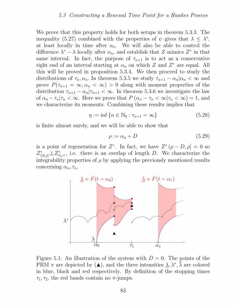
5.3 Constructing a Renewal Time Point for a Hawkes Process

We prove that this property holds for both setups in theorem 5.3.3. Theinequality (5.27) combined with the properties of ψ gives that λ ≤ λ∗,at least locally in time after αn. We will also be able to control thedifference λ∗ − λ locally after αn, and establish that Z mimics Z∗ in thatsame interval. In fact, the purpose of τn+1 is to act as a conservativeright end of an interval starting at αn on which Z and Z∗ are equal. Allthis will be proved in proposition 5.3.4. We then proceed to study thedistributions of τn, αn. In theorem 5.3.5 we study τn+1 − αn|αn < ∞ andprove P (τn+1 = ∞, αn < ∞) > 0 along with moment properties of thedistribution τn+1 − αn|τn+1 <∞. In theorem 5.3.6 we investigate the lawof αn− τn|τn <∞. Here we prove that P (αn − τn <∞|τn <∞) = 1, andwe characterize its moments. Combining these results implies that

η := inf n ∈ N0 : τn+1 =∞ (5.28)

is finite almost surely, and we will be able to show that

ρ := αη +D (5.29)

is a point of regeneration for Z∗. In fact, we have Z∗ (ρ−D, ρ] = 0 soZ∗|(0,ρ] |= Z∗αη+, i.e. there is an overlap of length D. We characterize the

integrability properties of ρ by applying the previously mentioned resultsconcerning αn, τn.

λ∗

α0

λ

λ+ F (t− α0)

τ1 α1

λ+ F (t− α1)

Figure 5.1: An illustration of the system with D = 0. The points of thePRM π are depicted by (N), and the three intensities λ, λ∗, λ are coloredin blue, black and red respectively. By definition of the stopping timesτ1, τ2, the red bands contain no π-jumps.

83


The precise result is as follows: Define F∗t = σ(Ft, π↑λ,λ

). It is clear

that (F∗t ) defines a filtration and without changing notation, we extendit to satisfy the usual hypothesis.

Theorem 5.3.2.Grant either setup (AD) or (O).

1. The random time ρ = αη +D is an a.s. finite F∗t -stopping time.

2. The random measure π↓λ,λ is an F∗t -PRM and hence π↓λ,λ |= F∗ρ .Moreover, we have Z∗ρ+ = Zρ+ and independent of Z∗|(0,ρ]. In partic-

ular, Z∗ρ+ is distributed as an ADHP with weight h, rate ψ, initialage D and signal t 7→ −f (t+D).

3. It holds that E (ρ− α0)p < ∞. Under assumption 5.3(B) it holds

that ρ− α0 has exponential moment.

To prove Theorem 5.3.2 we establish the results below and combinethem in the end. The proofs of these results, and the main result, may befound in the proof section.

Theorem 5.3.3.h

1. Consider setup (AD). It holds that αn, n ∈ N satisfies (5.27). More-over, assume ZI from example 5.2.5 exists, and assume only thatassumption 5.1 and assumption 5.3 (A) holds with r = f . Thenassumption 5.2 is satisfied for Z∗ = ZI and

αI0 = infi > 0 : θi−jN (−1, 0] ≤ γ (j) , j ≥ 0

. (5.30)

2. Consider setup (O) and recall ψL from (5.6). It holds that αn, n ∈ Nsatisfies (5.27). Moreover, assume ZI from example 5.2.5 exists,and assume only that assumption 5.1 and assumption 5.3 (A) holdswith r = f . Define Z0 as the stationary linear Hawkes process drivenby π with weight/rate h+, ψL (see [5] theorem 1 and remark 8). Thenassumption 5.2 is satisfied with

αI0 = infi > 0 :

∫ i

−∞h+ (t− s) dZ0

s ≤ f(t− i)− r(t− i) ∀t > i. (5.31)

84

5.4 Hawkes Processes In a Markov Chain Framework

Proposition 5.3.4.Under either setup it holds a.s. for all n ∈ N0 such that αn < ∞ andt ∈ (αn, τn+1] that

Z|(αn,τn+1) = Z∗|(αn,τn+1) (5.32)

and

0 ≤ λ∗t − λt ≤ F (t− αn). (5.33)

Theorem 5.3.5.Under either setup it holds that

P (τn − αn−1 =∞|αn−1 <∞) = exp (−‖F‖L1) (5.34)

P (τn − αn−1 ≤ t|τn <∞) =1− exp

(−∫ t

0 F (s) ds)

1− exp (−‖F‖L1). (5.35)

In particular the conditional distribution τn − αn−1|τn < ∞ has p’th mo-ment. Under assumption 5.3 (B) it has exponential moment.

It turns out that the αn’s defined above may be analyzed using adiscrete Markov chain. In fact one may rewrite αI0 and αn − τn as returntimes to state 0 for a specific Random Exchange process (see Appendix).This yields precise distribution results as given in the next proposition.

Theorem 5.3.6.Under either setup it holds that αI0 and (αn − τn) | (τn < ∞) have p’thmoment. If also assumption 5.3 (B) holds then these laws have exponentialmoment.

5.4 Hawkes Processes In a Markov ChainFramework

In this section we first apply theorem 5.3.2 iteratively to obtain consec-utive renewal time points ρi, which partition Z∗ into independent bits.

85


Afterwards, we construct a Markov chain that contains the informationof Z∗, and where the ρi’s acts as the return times to an atom. The pur-pose is to use Markov chain theory to obtain results for Z∗, which we doin the next section.

Choose D > 0 and set ρ0 := ρ, π0 := π, π0 := π and π1 = π↓λ,λρ0+ . Wealso introduce another auxiliary PRM π1 independent of π0, π0, π1. Notethat π1, π1 are F1

t -PRMs where F1t = σ(F∗ρ , π1

|(0,t], π1|(0,t]). It holds that Z∗ρ+

is an ADHP driven by π1 with R : t 7→ −f (t+D), A0 = D. In particularα1

0 = 0 satisfies (5.27) already. Thus, π1, π1 and α10 induces a new renewal

system as in section 3. From there we obtain sequences(α1i

),(τ 1i

)and

two new PRMs which we denote π↓1, π↑1. Applying theorem 5.3.2 on thissystem gives a new renewal time ρ1.

Continuing this way gives sequences(πi),(πi),(π↑i),(π↓i), (ρi). If we

set %i =∑i

j=0 ρj, we have that

B 7→ Z∗ ((%i−1 −D, %i] ∩ (B + %i−1)) , B ∈ B(−D,∞) (5.36)

are i.i.d. for i ∈ N, each being the Hawkes process initialized with A0 = D,R : t 7→ −f (t+D) and driven by πi.

In fact, we can study Z∗ from a Markov chain perspective. Define

ρ− (t) = sup s < t : ∃i ∈ N0 : s = %i , (5.37)

J (n) = |j ∈ N0 : %j < n| , (5.38)

and Aρt = t− ρ− (t). Consider the stochastic processes on the state-space

M cR2

+×M c

R2+× N,

Φpren =

(π↓J(n)

|(0,Aρn], π↑J(n), Ap

n

)(5.39)

Φn = θρ0Φpren (5.40)

for n ∈ N. In this framework, Theorem 5.3.2 states that Φn |= Φpre0 , . . . ,Φpre

ρ0.

Using (5.26) we may construct a map H∗ : M cR2

+×M c

R2+× N → M c

(−D,0]

satisfying H∗ (Φn) = (θρ0+nZ∗)|(−D,0]. Also, by construction of ρi, the in-

dicator function J (n+ ρ0 + 1)− J (n+ ρ0) may be written as some mapHJ (Φn). It follows that Φ is a Markov chain with an atom

Ξ = µ, ν, n : HJ (µ, ν, n) = 1 . (5.41)

86

5.5 Applications

Consider the subspace

X =µ, ν, n : µ, ν are simple , PΦ

µ,ν,n (Φ hits Ξ eventually) = 1

(5.42)

and let PΦ be the kernel of Φ. By definition of X, any chain with kernelPΦ started in X eventually hits Ξ, and by theorem 5.3.2 Φ almost surelyreturns to Ξ once hitting it. Thus X is an absorbing state for chain Φ, andwe shall from now on always refer to Φ, PΦ as the restricted kernel to X(see proposition 4.2.4. [34]). Since Ξ is an accesible atom for this chain,it is irreducible (Prop. 5.1.1 [34]) and aperiodic. The return time to Ξ isdistributed as ρ1, so by Kac’s theorem it follows that PΦ is positive withinvariant law P for p ≥ 1. Not surprisingly it turns out that P agreeswith ZI from example 5.2.5 with parameters h, ψ, whenever they bothexist.

Proposition 5.4.1.Assume that p ≥ 1 and ZI from example 5.2.5 exist with coupling proper-

ties as given in the example. It holds that H∗(P)

D= ZI

|(−D,0].

5.5 Applications

In this section we apply the Markov chain construction from section 5.4to establish asymptotic results for Z∗. We show distribution results of thecoupling time. Then we present a functional CLT, a time-average CLT,and a LIL for Z∗.

5.5.1 Bound On The Coupling Time

In [5] it was shown that two ordinary Hawkes processes, started with differ-ent initial conditions couple under regularity conditions. In the previouschapter we showed a similar statement for ADHPs. Our construction ofρ confirms these results and provide moment results for these couplingtimes. More preciesly, we have the following proposition.

Proposition 5.5.1.Let Z∗1, Z∗2 be two π-driven ADHPs initialized with A∗10 , A

∗20 and signals

R∗1t , R∗2t . Assume that α0 satisifies assumption 5.2 for both measures si-

multaneously.

87


Define the coupling time T = inft > 0 :

∣∣Z∗1 − Z∗2∣∣ (t,∞) = 0

. Itholds that T ≤ ρ and in particular that (T − α0)+ has p’th moment. Underassumption 5.3 (B), (T − α0)+ has exponential moment.

Proof.By theorem 5.3.2 2) we have Z∗1ρ+ = Z∗2ρ+ = Zρ+. The moment resultsfollows from theorem 5.3.5 and theorem 5.3.6.

5.5.2 Asymptotics

The Markov chain Φn from (5.39) can be used to establish various asymp-totic results for Z∗ in a general setting. Let G : M c

R2+×M c

R2+×N→ R be

a measurable function which we normalize with G = G− PG where P isthe invariant measure from proposition 5.4.1. We shall discuss asymptoticresults of the sum

Sn(G)

=n∑k=1

G (Φprek ) (5.43)

provided of course that G is a function s.t. G (Φpren ) is a well-defined

variable for all n ∈ N. Define

Sn(G)

= Sn+ρ0 − Sρ0. (5.44)

Theorem 5.5.2.Assume that p ≥ 2. Define µρ = Eρ1 and

σ2 = µ−1ρ ESρ1

(G)2. (5.45)

Assume that σ2 is finite and nonzero.

1. The following CLT holds

n−1/2Sn(G)⇒ N

(0, σ2

). (5.46)

2. The following LIL holds: Almost surely,

lim infn→∞

Sn(G)

√2σ2n ln lnn

= −1, lim supn→∞

Sn(G)

√2σ2n ln lnn

= 1. (5.47)

88

5.5 Applications

Define St(G)

for t ∈ (n, n+ 1) as the linear interpolation between Sn(G)

and Sn+1

(G), and put

Bnt =

1√nσ2

Snt(G). (5.48)

The following functional CLT holds

Bn(·) ⇒ B(·) (5.49)

where B is the 1-dim Brownian motion, and the convergence (⇒) is indistribution in the D space on [0,∞). See [4] chapter 3.

Proof.A direct application of theorem 17.2.2, theorem 17.4.4, and section 17.4.3[34] on Φn gives the desired results for Sn in place of Sn. Standard argu-ments extend these results to hold for Sn as well.

Example 5.5.3.We give two applications of theorem 5.5.2.

1. Take G (µ) =∫ 0

−D φ (s) dH∗ (µ) (s) where φ : (−D, 0] → R is abounded map. In particular, when φ ≡ 1, D = 1, we obtain

Sn(G)

= Z∗ (0, n]− EZI (0, n] . (5.50)

It is straightforward to show a sufficient criteria for σ2 <∞ is that eitherp > 2 in the (O) setup or p ≥ 2 in the (AD) setup. Also it is easy to seethat for non-degenerate choices of h, ψ we have σ2 > 0.

2. Fix m ∈ N, and let T : M c|(−m,0] → R be a measurable map. Take

D = m+ 1 and G (µ) =∫ 1

0 T(

(θsH∗ (µ))|(−m,0]

)ds. These choices lead to

Sn(G)

=

∫ n

0

T(θsZ∗|(s−m,s]

)ds− nET

(ZI|(−m,0]

). (5.51)

To obtain σ2 <∞ we need a growth condition depending on the setup:

89


(AD) ∃c, C > 0 : |T (µ)| ≤ C exp (cµ (−m, 0]) (5.52)

(O) ∃C > 0 : |T (µ)| ≤ C

∣∣∣∣ µ (−m, 0]

1 + ln (µ (−m, 0])

∣∣∣∣p/2−1

. (5.53)

Consider first setup (AD). Recall that

Z∗ρ0+ (n−D,n] = Zρ0+ (n−D,n] ≤ Dδ−1 + π↓λ,λρ0+ (n−D,n]× [0, K] .

(5.54)

It follows that

sups∈(n−1,n]

∣∣T (θ−sZ∗|(s−m,s])∣∣ ≤ C exp(cDδ−1

)exp

(cπ↓λ,λρ0+ (n−D,n]× [0, K]

):= Yn

For j = 1 . . . D, n ∈ N define Y jn = Yn if n ≡ j mod D, and otherwise

set Y jn as an i.i.d. copy of Y1. Indeed by the Cp-inequality there is some

possibly larger C > 0 s.t.

Sρ1 (G)2 ≤ C

D∑j=1

(ρ1∑n=1

Y jn

)2

(5.55)

Notice that for each fixed j = 1, . . . , D, the sequence Y jn , n ∈ N is i.i.d. It

follows from theorem 5.2, chapter 1 in [21] that σ2 <∞.

Consider now setup (O), and take γ (t) = C ln+ t for C so large that(5.15) is satisfied. Note that x 7→ x/ ln (x+ 1) is increasing for x > 0 so

sups∈(%0,%1]

∣∣∣T (θ−sZ∗|(s−m,s])∣∣∣ ≤ C

∣∣∣∣ Z∗ (%0, %1]

ln (1 + Z∗ (%0, %1])

∣∣∣∣p/2−1

. (5.56)

Notice that for our choice of γ, we have the inequality∫ x

0

γ (t+ 1) dt ≤ Cx ln (x+ 1)

for a possibly larger constant C > 0. From the definition of αn it followsthat

90

5.6 Discussion and Outlook

sups∈(%0,%1]

∣∣∣T (θ−sZ∗|(s−m,s])∣∣∣ ≤ CT

∣∣∣∣ Cρ1 ln (ρ1 + 1)

ln (1 + Cρ1 ln (ρ1 + 1))

∣∣∣∣p/2−1

≤ CTCρp/2−11

(5.57)

again for a possibly larger constant C > 0. From here it follows thatσ2 < ∞. One would have to check σ2 > 0 for the given T , but for mostpractical applications, this is a triviality.

5.6 Discussion and Outlook

In the following, we shall discuss generalizations and limitations of thepresented results, and suggest further research topics.

Multivariate Hawkes Processes

It is straight forward to generalize the regeneration procedure to a mul-tivariate Hawkes Process with N units (see [12],[13] or chapter 2 for anintroduction to these). One should split each πi , i ≤ N into π↑i, π↓i fori = 1, ..., N - analogous to what was done in the start of section 3.1. Theτ in’s should be generalized in the obvious way, while αn should be mod-

ified so that it ensures that∑N

i=1

∣∣∫ αn0 hij (t− s) dZi

s +Rit

∣∣ ≤ f (t− αn) .In setup (AD) this is achieved by substituting π↓λ,λ in (5.25),(5.31) with∑N

i=1 π↓i which will be a PRM with mean intensity N dzds. In setup

(O), the clusters Z i should be dominating linear N -dimensional Hawkesprocesses. While the total progeny distribution of Z i is no longer Boreldistributed, it is well known that it has exponential moment, which issufficient to complete the proof.

Stability For More General Setups

A significant observation is that the setups (AD) and (O), essentially onlyaffect the construction of ρ through the choice of α’s and f . For otherand more general setups in the univariate or multivariate case, one mayadapt this procedure to establish stability regimes. For example it mightbe a method to explore other multivariate systems where inhibition fromeither the weight or the age have a potential effect on the stability regime.

91


Optimizing the Regeneration Scheme And Improving Results

These results establish a regeneration scheme for weight functions h s.t.∫∞0 |h (t)| tp+1 ln+ tdt <∞. However, invariant solutions to Z exist already

for h with first moment i.e.∫∞

0 t |h (t)| dt < ∞. Also, the CLT result forordinary Hawkes processes by Zhu [44], assuming that h decreasing andpositive, only requires that t 7→ th (t) is integrable. This correspondsto p = 0, instead of p ≥ 2 which we require in theorem 5.5.2. Thesefacts indicate that there may exist renewal times with better momentproperties, than those discussed in this chapter.

Also, the main result in [19], developed simultaneously with the resultspresented in this paper, proves existence of a regeneration point withimproved integrability properties, in the case where the Hawkes process islinear with positive weight functions. Moreover, the exponential momentresults in [19] are more refined, primarily due to the use of renewal timesof a certain M/G/∞ queue with a deterministic service time instead ofrandom exchange processes.

Implementation and Practical Computation

While this chapter focuses on the theoretical development of regenerationtimes, the method is constructive and ρ may be simulated in either setup.It would be of interest to study the efficiency of this algorithm.

5.7 Proofs

5.7.1 Proofs of Section 2 Results

123Proof of Proposition 5.2.4To show the claimed result for f under assumption 5.3 (A), substitute the

92

5.7 Proofs

inner variable with u = s+ t and apply Tonelli to obtain∫ ∞0

∫ ∞0

tpγ (s+ 1)h (t+ s) dsdt =

∫ ∞0

∫ ∞t

tpγ (u− t+ 1)h (u) dudt

(5.58)

=

∫ ∞0

∫ u

0

tpγ (u− t+ 1)h (u) dtdu

(5.59)

≤ (p+ 1)−1

∫ ∞0

up+1γ (u+ 1)h (u) du

(5.60)

which proves the desired. Under assumption 5.3 (B) it is straightforwardto show that f has exponential moment. The claimed result for F p, Ffollows immediately.

5.7.2 Proofs of Section 3.1 Results

123Proof of Theorem 5.3.31. We claim for n ∈ N that∣∣∣∣∫ αn

0


∣∣∣∣ ≤ f (t− αn) ∀t > αn (5.61)

if αn <∞. We prove this by induction over n ∈ N0. The induction startn = 0 is per assumption 5.2. To prove the induction step, we split theintegral of interest∣∣∣∣∫ αn

0


∣∣∣∣ ≤ ∣∣∣∣∫ αn

αn−1

h (t− s) dZ∗s∣∣∣∣+

∣∣∣∣∫ αn−1

0


∣∣∣∣ .(5.62)

By the induction assumption, the 2nd term is bounded by f (t− αn−1)for all t > αn−1. The first term above can be split up to whether jumpsof Z∗ happen when A∗t ≤ δ or not∫ αn

αn−1

1 As ≤ δh (t− s) dZ∗s +

∫ αn

αn−1

1 As > δh (t− s) dZ∗s . (5.63)

93


Consider the first term. By the (AD) criteria we have∫ b

a

1 As ≤ δ dZ∗s ≤ πK (a, b] :=

∫(a,b×[0,K]

dπ (s, z) . (5.64)

On the interval t ∈ (αn−1, τn), we have per definition of τn thatN [t, t] ≥ πK [t, t] while for t ∈ (τn, αn] we have πK [t, t] = N [t, t]. Itfollows that for t > αn, we have∫ αn

αn−1

1 As ≤ δh (t− s) dZ∗s (5.65)

≤∫ αn

αn−1

h (t− s) dπKs (5.66)

≤h (t− τn) +

∫ αn

αn−1

h (t− s) dNs (5.67)

≤h (t− αn) +

αn−αn−1−1∑i=0

γ (i)h (t− αn + i) (5.68)

≤∫ αn−αn−1−1

0

γ (s+ 1)h (t− αn + s) ds+ (1 + γ (0))h (t− αn) . (5.69)

For the second integral in (5.63), recall that δ−1 ∈ N and notice that theinterdistance between jumps of Z∗ with As > δ is at least δ per definition.We obtain the bound∫ αn

αn−1

1 As > δh (t− s) dZ∗s (5.70)

≤(αn−αn−1)δ−1−1∑

i=0

h (t− αn + iδ) (5.71)

≤(αn−αn−1)−1∑

j=0

δ−1h (t− αn + j) (5.72)

≤∫ αn−αn−1−1

0

δ−1h (t− αn + s) ds+ δ−1h (t− αn) . (5.73)

The sum of the two right-hand sides of (5.69) and (5.73) are less thanf (t− αn, αn − αn−1 − 1)− r(t−αn). The induction claim now follows byinserting this back into (5.62).

94

5.7 Proofs

To prove that αI0 satisfies assumption 5.2, repeat the proof above with−∞ in place of αn−1 and αI0 in place of αn. We omit the details.

2. Consider now the (O) setup. We claim again for n ∈ N that∣∣∣∣∫ αn

0


∣∣∣∣ ≤ f (t− αn) ∀t > αn. (5.74)

As before we proceed by induction over n ∈ N0. The induction startfollows from assumption 5.2. Assume now the claim holds for n − 1. Bythe induction assumption and the definition of f we have

∣∣∣∣∫ αn

0


∣∣∣∣ ≤ ∣∣∣∣∫ αn

αn−1

h (t− s) dZ∗s∣∣∣∣+ f (t− αn−1) . (5.75)

It is seen per induction over jumps of Zn, that

Zn [s, s] ≥ Z∗ [αn−1 + s, αn−1 + s]

for all s ∈ (αn−1, αn]. Hence

∣∣∣∣∫ αn

αn−1

h (t− s) dZ∗s∣∣∣∣

≤∣∣∣∣∫ αn−αn−1

0

h (t− s) dZns

∣∣∣∣≤f(t− αn, αn − αn−1 − 1)− r (t− αn) (5.76)

inserting back into (5.75), and using the definition of f gives the desiredresult.

The statement about αI0 is a direct implication of the claim thatZI [t, t] ≤ Z0 [t, t] for all t ∈ R almost surely. To prove this claim, letZ1, Z2 be Hawkes processes with weight h+, h and rate functions ψL, ψrespectively, with common intialization R ≡ 0, A0 = 0. By the couplingproperty from example 5.2.5 We have almost surely thatZ0|[t,∞) = Z1

|[t,∞), ZI|[t,∞) = Z2

|[t,∞) for t large enough. On the other hand, per

95


induction over jumps of Z1 it is straightforward to prove thatZ1 [t, t] ≥ Z2 [t, t] for all t ∈ R+ so it follows that almost surelyZ0 [t, t] ≥ ZI [t, t] eventually. The claim now follows from the fact that(Z0, ZI

)is stationary and ergodic.

Proof of Proposition 5.3.4

Define Z = |d (Z∗ − Z)| and let A be its age process. We have fort ∈ (αn−1, τn]

X∗t −Xt =

∫ t−

αn−1

h (t− s) d(Z∗s − Zs) +

∫ αn−1

0

h (t− s) dZ∗s +R∗ (t)− f (t− αn−1) .

(5.77)

Applying (5.27) gives∣∣∣∣∫ αn−1

0

h (t− s) dZ∗s +R∗ (t)− f (t− αn−1)

∣∣∣∣ ≤ 2f (t− αn−1) . (5.78)

Define for n ∈ N

τ ∗n = inft > αn−1 : Z [t, t] = 1

. (5.79)

We claim that τ ∗n ≥ τn almost surely. Notice that A∗t ≥ At fort ∈ (αn−1, τ

∗n]. For all t ∈ (αn−1, (αn−1 +D) ∧ τ ∗n] we combine (5.27)

and (5.5) to see that

0 = λt ≤ λ∗t ≤ cψ + Lf(t− αn−1) ≤ F (t− αn−1) (5.80)

which shows that τ ∗n ≥ τn ∧ (αn−1 +D) . For all t in the (possibly empty)interval (αn−1 +D, τ ∗n] we have

X∗t =

∫ t−

αn−1

h (t− s) dZ∗s +

∫ αn−1

0

h (t− s) dZ∗s +R∗t (5.81)

≥∫ t−

αn−1

h (t− s) dZ∗s − f (t− αn−1) (5.82)

= Xt. (5.83)

Since ψ is increasing we get the following inequality

ψ (Xt, At) ≤ ψ (X∗t , A∗t ) for all t ∈ (αn−1 +D, τ ∗n]. (5.84)

96

5.7 Proofs

If A∗t > At the definition of τ ∗n gives that A∗t , At ≥ t − αn−1. Therefore(5.77) and (5.78) give

ψ (X∗t , A∗t )− ψ (Xt, At) ≤ L (X∗t −Xt) + cψg (t− αn−1) (5.85)

≤ 2Lf (t− αn−1) + cψg (t− αn−1) (5.86)

≤ F (t− αn−1) . (5.87)

Likewise, if A∗t = At we have

ψ (X∗t , A∗t )− ψ (Xt, At) ≤ L (X∗t −Xt) . (5.88)

By definition of τn, this implies τ ∗n ≥ τn. Thus, in between two consecutiveτ stopping times, the two Hawkes processes agree.

Proof of Theorem 5.3.5The results (5.34),(5.35) are straightforward consequences of the strongMarkov Property and [5] lemma 1. The density of the conditional distri-bution τn − αn−1|τn <∞ is proportional to

F (t) exp

(−∫ t

0

F (s) ds

)≤ F (t) (5.89)

which shows the desired moment results for the distribution .

Proof of Theorem 5.3.6To structure the proof, we discuss the following four variables, in writtenorder

1. αI0 in the (AD) setup

2. αn in the (AD) setup

3. αI0 in the (O) setup

4. αn in the (O) setup

1. To study αI0, we introduce the process Mi for i ≥ 0 given by

Mi = infm ≥ 0 : θi−jN (−1, 0] ≤ γ (j +m) , j ≥ 0

(5.90)

= infm ≥ 0 : θkN (−1, 0] ≤ γ (i+m− k) , k ≤ i

. (5.91)

97


In words, the value Mi is the minimum number of units the functionj 7→ γ (i+ j) must be shifted before it bounds πK on all intervals(i− j − 1, i− j], j ∈ N0, see fig. 5.2.

ii− 1i− 2i− 3i− 4Mi

s 7→ γ (i+Mi − s)

πK(i− j − 1, i− j]

Figure 5.2: An illustration of Mi.

We see that α0 = inf i > 0 : Mi = 0 i.e α0 is the first time Mi hits0. Notice that M0 is a well-defined random variable by a Borel-Cantelliargument. Observe also that M is in fact an RE-process with updatescheme

Mi = (Mi−1 − 1) ∨ dγ−1 (N (i− 1, i])e. (5.92)

By corollary 7.4.3 M has a unique invariant distribution µ and since

Nd= θ1N it follows that M0

d= M1 ∼ µ. The result follows from corol-

lary 7.4.3 part 2.

2. Notice that αn−τn has p’th-moment / exponential moment iff αn−dτnehas as well. For any realization such that τn <∞ we may write

αn − dτne = infi > 0 : θi−j+dτn−αn−1eNαn−1+ (−1, 0] ≤ γ (j) , j = 0, . . . , i+ dτn − αn−1e − 1

.

(5.93)

We now proceed as previously. Define M ′i for i ≥ 0 as the process

M ′i = inf

m ≥ 0 : θi−j+dτn−αn−1eNαn−1+ (−1, 0] ≤ γ (j +m) , j = 0, . . . , i+ dτn − αn−1e − 1

.

(5.94)

Notice that αn − dτne is the first time M ′i hits 0. From theorem 7.3.1 we

have π↑λ,λαn−1+ |= π↓λ,λαn−1+ and thus τn−αn−1 is independent of Nαn−1+. Observealso that M ′ is an RE-process defined by

M ′i = (M ′

i−1 − 1) ∨ dγ−1(Ndτne+ (i− 1, i]

)e. (5.95)

98

5.7 Proofs

To study the distribution of M ′0 note that it may be described as M ′′

αn−dτnewhere M ′′ is another RE-process defined by M ′′

0 = 0 and

M ′′i = (M ′′

i−1 − 1) ∨ dγ−1(Nαn−1+ (i− 1, i]

)e. (5.96)

Let P ∗ be the conditional distribution of dτn − αn−1e given τn <∞. If φis a positive increasing function and

(P kx

)is the k-step Markov kernel for

M ′′ then

E (φ (M ′0) |τn <∞) =

∫ ∫φ (y) dP k

0 (y) dP ∗ (k) (5.97)

≤∫φ (y)µ (y) +

∫ ∫φ (y) d

∣∣P k0 − µ

∣∣ (y) dP ∗ (k) .

(5.98)

From theorem 14.1.4 [34] it follows that if µ (φ) < ∞, then the secondterm above is finite. The desired result now follows from theorem 5.3.5and corollary 7.4.3.

3. We now analyze αI0 under setup (O). Here we utilize that the lawof the stationary Linear Hawkes process Z0 has a cluster process repre-sentation which we now describe; Let N be a Poisson process on R withintensity cψ and for i ∈ Z let (Zi) be independent Hawkes processes withweight/rate h+, x 7→ Lx and initialized with a single jump at t = 0 (i.e.Zi [0, 0] = 1 and Ri

t = h+ (t)). Define now

Z(A) =∑i∈Z

Ci (A) (5.99)

where Ci is a random measure given by Ci (A) = Zi (A− si) and si is thei’th jump of N for i ∈ Z (with convention s1, s2, ... being the first jumpsafter t = 0, and s0, s−1, ... being the most recent jumps before t = 0). ThenZ is distributed as the stationary linear Hawkes process with weight/rateh+/ψL. See [11],[41] for more details on this construction. It follows that

αI0D= α0 where

α0 = infi > 0 :

∣∣∣∣∫ i

−∞h+ (t− s) dZs

∣∣∣∣ ≤ f(t− i)− r(t− i),∀t > i.

(5.100)

99


We shall use the following fact, coming from section 1.1 in [41] andthe proof of proposition 1.2 in same refrence: We may assume that theclusters Z i are constructed s.t. there is i.i.d. (Wi, Xi,j), also independent

of N such that Wi |= Xi,j, Xi,j ∼ ‖h+‖−1L1 h+(t) dt and

Zi(R) = Zi(−∞, Yi] = Wi, (5.101)

where Yi =∑Wi

j=1Xi,j and W1 is distributed as the total progeny of a Pois-

son branching process, with mean offspring ‖h+‖−1L1 .

By the Otter-Dwass formula (see [16]) The p.m.f. of W1 is

pW (n) =nn−1

‖h+‖L1 n!en(−‖h+‖L1+ln‖h+‖L1). (5.102)

The stirling approximation for n! gives that

E exp (cW ) <∞⇐⇒ c ≤ ch = ‖h+‖L1 − ln+ ‖h+‖L1 − 1 (5.103)

If assumption 5.3 (B) holds, take any c0 > 1. Otherwise, let c0 > 1 be aconstant satisfying γ (t) ≥ c0 (p+ 1) c−1

h ln+ t for t sufficiently large. De-fine γ∗ (t) = c−1

0 γ(c−1

0 t− 1)

when c−10 t ≥ 1 and γ∗ (t) = 0 otherwise.

With Nt := N [0, t] for t > 0 and −N(t, 0) otherwise we define

Y i =Ni

maxl=Ni−1+1

Yl, W i =

Ni∑l=Ni−1+1

Wl, (5.104)

α0 = infi > 0 : Y i−j ≤(1− c−1

0

)j, W i−j ≤ γ∗ (j) , j ≥ 0. (5.105)

We claim that α0 ≤ α0. This follows from the calculations for t > α0∫ α0

−∞h+(t− s)dZs =

∞∑j=0

∫ α0−j

α0−j−1

∫ t

s

h+(t− u)dCNs(u)dNs (5.106)

Note that (5.101) implies that for all clusters CNs with s ∈ (α0 − j − 1, α0 − j]we have Supp (CNs) ⊂

[s, s+ Y α0−j

]. By the inequalities obtained from

the definition of α0 we have[s, s+ Y α0−j

]⊂[s, α0 − c−1

0 j]. Since h+ ≤ h

and h is decreasing we conclude that h (t− u) ≤ h(t− α0 + c−1

0 j)

for

100

5.7 Proofs

all u ∈ Supp (CNs) , s ∈ (α0 − j − 1, α0 − j] , t > α0. Inserting this into(5.106) gives∫ α0

−∞h+(t− s)dZs ≤

∞∑j=0

h(t− α0 + c−10 j)

∫ α0−j

α0−j−1

CNs[s, α0 − c−10 j]dNs.

(5.107)

≤∞∑j=0

h(t− α0 + c−10 j)W α0−j (5.108)

Again, by the inequalities defining α0 we get∫ α0

−∞h+(t− s)dZs ≤

∫ ∞0

h(t− α0 + c−10 s)γ∗(s+ 1)ds+ h(t− α0)γ

∗(0)

(5.109)

≤∫ ∞

0

h(t− α0 + s)γ(s+ 1)ds+ h(t− α0)γ(0)

(5.110)

≤ f(t− α0)− r(t− α0) (5.111)

which proves the claim.To describe the moment of α0 define

Mi = infm ≥ 0 : Y i−j ≤

(1− c−1

0

)(j +m) , W i−j ≤ γ∗ (j +m) , j ≥ 0

.

(5.112)

Indeed, M0 <∞ by a Borel-Cantelli argument. As before α0 is the returntime to 0 for the RE-process Mi with update-variables

d((

1− c−10

)−1Y i

)∨ (γ∗)−1 (W i

)e

and started at M0, carrying the invariant distribution of M . Under as-

sumption 5.3 (A) we have (γ∗)−1 (t) ≤ exp(ch (p+ 1)−1 t

)for t large. It

follows that the update variables have (p+ 1)th moment and the startingdistribution has p’th moment, so it follows from corollary 7.4.3 that α0 hasp’th moment. Likewise, under assumption 5.3 (B) the update variableshave exponential moment and the starting distribution has exponentialmoment as well. It follows from corollary 7.4.3 that α0 has exponential

101


moment.

4. We now analyze αn under setup (O). To outline the similarity weshall re-use some of the notation from the previous proof, but for slightlymodified random variables.

Notice that Zn[t, t] is dominated by the Hawkes process Z ′ with thesame weight function h+, rate function ψL and initial signalR′t = f(t−btc) +h+(t− (τn − αn−1)). The law of Z ′ has a cluster processrepresentation given as follows:Let N be an inhomogeneous Poisson process with intensity cψ+Lf(t−btc),and let ξ ∼ (τn−αn−1) | (τn <∞). Define Zi as before, and let Ci, C

ξ bethe mutually independent clusters given by Ci(A) = Zi(A − si) where siis the ith jump of N for i ∈ N, and Cξ(A) = Z−1(A− ξ). Define

Z(A) =∞∑i=0

Ci(A) + Cξ(A), A ∈ BR+. (5.113)

Then ZD= Z ′ and hence also

(αn − αn−1 | τn <∞) (5.114)

D

≤ inf

i > dξe :

∣∣∣∣∫ i

0

h+ (t− s) dZs

∣∣∣∣ ≤ f (t− i, i− 1)− r(t− i),∀t > i, Z [0, i] ≤∫ i

0

γ (s+ 1) ds

(5.115)

whereD≤ denotes inequality in the usual stochastic order(see [3] chap-

ter 2). As before, we have i.i.d. variables (Wi, Xi,j), (Wξ, Xξ

j ) and also

independent of N, ξ such that Xi,j ∼ ‖h+‖−1L1 h(t) dt, Wi ∼ Z0(R) and

Zi(R) = Zi(−∞, Yi] = Wi, ∀i ∈ N (5.116)

Z−1(R) = Z−1(−∞, Y ξ] = W ξ (5.117)

where Yi =∑Wi

j=1Xi,j and Y ξ =∑W ξ

j=1Xξj . Define now

Y i =Ni

maxl=Ni−1+1

Yl, W i =

Ni∑l=Ni−1+1

Wl (5.118)

102

5.7 Proofs

and notice that (Y i,W i) for i ∈ N is an i.i.d. sequence. Define now c0, γ∗

as previously and set

ζ = infi > 0 : Y i+dξe−j ≤(1− c−10

)j, W i+dξe−j ≤ γ∗ (j) ∀j ∈ 0, ..., i+ dξe − 1 \ i,

(5.119)

Y dξe ∨ Y ξ ≤(1− c−10

)i, W dξe +W ξ ≤ γ∗ (i). (5.120)

Define now the random time ζ s.t. ζ + dξe is equal to (5.115). We claimthat ζ ≤ ζ. To prove this, we apply similar arguments as in the part of3) where we showed thatα0 ≤ α0. By construction of Y i’s and ζ, it holds for alls ∈

(ζ + [ξ]− j − 1, ζ + dξe − j

)that Supp (CNs) ⊂

(−∞, ζ + dξe − c−1

0 j]

and this implies∫ dξe+ζ0

h+(t− s)dZs (5.121)

≤dξe+ζ−1∑j=0,j 6=ζ

h(t−(dξe+ ζ

)+ c−1

0 j)W dξe+ζ−j (5.122)

+h(t−(dξe+ ζ

)+ c−1

0 ζ)(W dξe +W ξ

)≤∫ dξe+ζ−1

0

h(t−(dξe+ ζ

)+ c−1

0 s)γ∗(s+ 1)ds+ h(t−(dξe+ ζ

))γ∗(0)

(5.123)

≤f(t−(dξe+ ζ

), dξe+ ζ − 1)− r(t− (ζ + dξe)). (5.124)

Likewise, the support constraint on CNs mentioned above must imply that

Z(0, ζ + dξe

]=

ζ+[ξ]−1∑j=0

Wj ≤ζ+dξe−1∑j=0

γ∗ (j) ≤∫ ζ+dξe−1

0

γ (s+ 1) ds.

(5.125)

This proves our claim. To analyze ζ define

Mi = infm ≥ 0 : Y i−j ≤

(1− c−10

)(j +m) , W i−j ≤ γ∗ (j +m) , j = 0, ..., i− 1

.

(5.126)

This is an RE-process started at M0 = 0 and with update variablesdmax(γ∗)−1(W i), (1 − c−1

0 )−1Y ie. As in the proof of 2) it follows that

103


M[ξ]−1 has p’th moment, and under assumption 5.3(B) it has exponentialmoment. The same therefore holds for the variable

M ′0 := (M[ξ]−1 − 1) ∨ dmax(γ∗)−1(W [ξ] +W ξ), (1− c−1

0 )−1Y [ξ] ∨ Y ξe.(5.127)

Now realize that ζ is the return time to 0 for the RE-process with updatevariables

d((

1− c−10

)−1Y i

)∨ (γ∗)−1(W i)e (5.128)

and started at M ′0. The desired result now follows from corollary 7.4.3

Proof of Theorem 5.3.2

1. To prove that ρ is a F∗ stopping time, we notice that

(ρ ≤ t) = (αη ≤ t−D) =

bt−Dc⋃i=0

(αη = i). (5.129)

So it suffices to show (αη = i) ∈ F∗i . Indeed, this is true since

(αη = i) =∞⋃k=0

(αk = i) ∩(∫ ∞

i

1z ≤ F (s)dπ↑λ,λ). (5.130)

2. By applying theorem 7.3.1 for each fixed t we see that π↓λ,λ is

an F∗t -PRM. The Strong Markov Property gives that π↓λ,λρ+ is a PRM in-dependent of F∗ρ . Notice now that Z+, λ+t := λρ+t is exactly the point

process and intensity of the ADHP driven by π↓λ,λρ+ with initial age D and

signal R : t 7→ −f (t+D). That is, Zρ+ is entirely generated by π↓λ,λρ+ andhence Zρ+ |= F∗ρ . Notice that Zρ+ = Z∗ρ+ by proposition 5.3.4 and thatZ∗|(0,ρ] ⊂ F∗ρ . It now follows that Z∗ρ+ |= Z∗|(0,ρ].

3. We introduce an i.i.d. sequence of random variables (βi) withdistribution β1 ∼ α1 − α0|τ1 − α0 < ∞. We then introduce anothersequence of random variables given by

βi =

αi − αi−1 i ≤ η

βi i > η.(5.131)

104

5.7 Proofs

Recall that (αj − αj−1)1≤j≤i are conditionally i.i.d. given τi < ∞. From

this we see that β is an i.i.d. sequence of variables distributed as β1, andwhich is also independent of η. We may now write

αη − α0 =

η∑i=1

αi − αi−1 (5.132)

=

η∑i=1

βi. (5.133)

From theorem 5.3.5 1) it follows that η is distributed as a negative bino-mial, and in particular it has exponential moment. To study the distri-bution of β1, we use that

α1 − α0 = (α1 − τ1) + (τ1 − α0) . (5.134)

Theorem 5.3.5 and theorem 5.3.6 give that β has p’th moment so thedesired result follows from theorem 5.2, chapter 1 [21]. Under assump-tion 5.3(B), one may conclude the proof by writing for small c > 0

E exp(cαη) = E exp(cα0) Eη∏i=0

exp(cβi) (5.135)

= E exp(cα0) E

[E

(η∏i=0

exp(cβi)∣∣ η)] (5.136)

= E exp(cα0) E(E exp(cβ1)

)η. (5.137)

Since η has exponential moment, the above expression is finite for smallc.

5.7.3 Proofs of Section 3.2 Results

123Proof of Proposition 5.4.1The proof is a coupling argument. Consider the Hawkes process Z∗ drivenby a fixed PRM π and started with R : t 7→ f (t+D) , A0 = D. Thenassumption 5.2 is satisfied with α0 = 0, r = −f. Thus, defining Φ as in(5.39) we have a coupling in the sense that (θnZ∗)|(−D,0] = H∗ (Φn) for

105


all n > ρ0. Since P is the invariant distribution of Φ the markov chain

converges in total variation and hence also H∗ (Φn) ⇒ H∗(P). On the

other hand, we have by the coupling property of ZI that almost surely,there is a random integer n0 s.t.(θnZ∗)|(−D,0] =

(θnZI

)|(−D,0]

for all n ≥ n0. It follows that

H∗ (Φn) = (θnZ∗)(−D,0] ⇒ ZI(−D,0] and the desired result follows from

uniqueness of limits.

106

Chapter 6

Mean-field Limit andPropagation of Chaos

In this chapter, we study a mean-field setup and associated mean-field lim-its. More precisely, we consider N interacting units which are organizedwithin K classes of populations. Each unit belongs to one of these classes,and any two units within the same class k are assumed to be similar,k = 1, . . . ,K. This means that they have the same rate function ψk,memory process Xk and initial signal Rk, and the weight function de-scribing the influence of any unit belonging to another class l is given byN−1hkl. However, each unit still has its own age process.

In this setup we establish a limiting distribution for a large scale net-work,N → ∞. Let Nk be the number of units in class k with proportionNk/N , and assume limN→∞Nk/N = pk > 0. We index the jth unitwithin class k by Zkj, k = 1, . . . ,K, j = 1, . . . , Nk. It is sensible toassume that small contributions from unit Z lj to the memory processXk of the kth class disappear in the large-scale dynamics, meaning thatN−1

∑Nlj=1

∫ t−0 hkl(t− s)Z lj(ds) ≈ pl

∫ t0 hkl(t− s)dEZ

l1(s) for large N , for

any 1 ≤ l ≤ K. Therefore, if a limiting point process(Zkj)j∈N exists, we

expect that any Zkj, k ≤ K, j ≥ 1 should have intensity

λkjt = ψk(xkt , A

kjt

),

where Akj is the age process of Zkj, and where the process xkt is deter-

6 Mean-field Limit and Propagation of Chaos

ministic, given by

xkt =K∑l=1

pl

∫ t

0

hkl (t− s) dEZ l1(s) + rkt ,

where rkt is a suitable limit of the initial processes in population k. Intheorem 6.2.2, we discuss criteria under which such a system exists. Oursecond main theorem, theorem 6.3.1, shows that this system will indeedbe a limit process for the generalized Hawkes processes for N → ∞.We also discuss in lemma 6.3.2 how robust the system is to adjustingthe weight functions. Not only is this robustness a good model featurein itself, but it also allows approximation of an arbitrary age dependentHawkes process, using weight functions with better features. Examplesare weight functions given by Erlang densities or exponential polynomialswhich induce Markovian systems, see [13].

6.1 Setup in This Chapter

In addition to the fundamental assumptions, we introduce the followingspecifications for the mean-field setup, which will be used throughout thissection. We partition the indices of individual units into K ∈ N differentpopulations, where K > 0. More precisely, for each fixed total populationsize N ∈ N,

Nk := Nk (N) := # i ≤ N : i in population k

will denote the number of units belonging to population k, 1 ≤ k ≤ K,and

N = N1 + . . .+NK.

We assume that each population represents an asymptotic part of all units,i.e., there exists pk > 0 such that

Nk

N

N→∞→ pk.

For a fixed N ∈ N, we re-index the N -dimensional age dependent Hawkesprocess of (2.15) as (

Zkj)k≤K,j≤Nk

,

108

6.2 The Limit System

where the superscript kj denotes the jth unit in population k. The weightfunction from the ith unit of population l to the jth unit of population kis given by N−1hkl. Moreover, all units within the same population havethe same spiking rate ψk. By taking L, cψ larger, we can and will assumethat (4.2) and (4.3) hold in the chapter as well. Finally, we assume thatall units in population k have the same initial signal Rk, and that theinitial ages are interchangeable in groups and mutually independent inand between groups. With this set of parameters, the age dependentHawkes process (Z,X,A) from (2.15) defined on t ∈ R+ becomes

Zkjt =

∫ t

0

∫ ∞0

1z ≤ ψk

(Xks , A

kjs

)dπkj (ds, dz) , j ≤ Nk, k ≤ K, (6.1)

Xkt =

1

N

K∑l=1

Nl∑j=1

∫ t−

0

hkl (t− s)Z lj(ds) +Rkt , k ≤ K,

where Akj is the age process of Zkj, starting from Akj0 at time t = 0.

Sometimes, to explicitly indicate the dependency on N, we add N to thesuperscript and write ZNki

t , XNk and ANki.

Model Observations

1. Suppose that the initial ages (Ai0)i∈N are exchangeable. Then the

symmetry of the system gives interchangeability between units within

the same population, i.e., Zkj L= Zki for i, j ≤ Nk, k ≤ K.

2. In the mean-field setup, all units within a population k share thesame memory process Xk.

6.2 The Limit System

We propose a limit system for N → ∞. To pursue this goal, take finitevariation functions t 7→ αkt , locally bounded functions t 7→ βkt , and PRMs

109


πk for k ≤ K, and consider the stochastic convolution equation

φkt =

∫ t

0

Eψk(xks , A

ks

)ds,

xkt =K∑l=1

pl

∫ t

0

hkl (t− s) dαls + βkt , (6.2)

Akt − Ak

0 = t−∫ t−

0

∫ ∞0

Aks1z ≤ ψk

(xks , A

ks

)πk (ds, dz) ,

with unknown (φ, x,A) =(φk, xk, Ak

)k≤K. Notice that only A is stochas-

tic. Introducing

Zkt =

∫ t

0

∫ ∞0

1z ≤ ψk

(xks , A

ks

)πk (ds, dz) ,

we can interpret Ak as age process of Zk. Hence, in the limit, the networkactivity can be resumed via the deterministic quantities xk, 1 ≤ k ≤ K,the only remaining randomness is in the individual age processes. Finally,notice that φ depends on the law of A.

We are motivated by what for the moment is a heuristic.

N−1Nk∑j=1

ZNkj ≈ pkEZk

for large N, where (Z1, . . . , ZK) denotes the limit process such that eachZk describes the jump activity of a typical unit belonging to populationk. This relation invites the idea that the memory process for N → ∞,t 7→ xt should satisfy the integral system (6.2) with φkt = αkt = EZk

t andβkt = ERk1

t . This motivates the following result.

Lemma 6.2.1.Let βt =

(βkt)k≤K be measurable and locally bounded. There is a unique

function α such that α = φ, where (φ, x,A) is the solution to (6.2). More-over, φ is continuous and x is bounded on [0, T ] by a constant C whichdepends on h :=

∑k,j |hkj|, ‖β‖T , T and L.

The proof is given in the proof section succeeding this one. Once thislemma is established, we can ensure existence of the limit process.

110

6.3 Large Network Asymptotics and Weight Approximations

Theorem 6.2.2.Let βt =

(βkt)k≤K be measurable and locally bounded. There is a unique

solution (Z,A) to the integral equation

Zkt =

∫ t

0

∫ ∞0

1

z ≤ ψk

(K∑l=1

pl

∫ s

0

hkl (s− u) dEZ lu + βks , A

ks

)πk (ds, dz) , 1 ≤ k ≤ K,

where Ak is the age process corresponding to Zk, initialized at Ak0.

Proof. Let (φ, x,A)k≤K be the tuple given in Lemma 6.2.1. Define thecounting process

Zkt :=

∫ t

0

∫ ∞0

1z ≤ ψk

(xks , A

ks

)πk (ds, dz) .

It is clear thatAk is the age process of Zk, and since dEZkt = Eψk

(xkt , A

kt

)dt,

Zk will satisfy the desired identity. For uniqueness, consider another so-

lution(Zk, Ak

)k≤K

, which satisfies the same identity :

Zkt =

∫ t

0

∫ ∞0

1

z ≤ ψk

( K∑l=1

pl

∫ s

0

hkl (s− u) dEZ lu + βks , A

ks

)πk (ds, dz) .

Defining xkt =∑K

l=1 pl∫ t

0 hkl (t− s) dEZlu+β

kt and φkt =

∫ t0 Eψ

k(xks , A

ks

)ds,

we note that EZkt = φkt . Thus, if we insert α = φ in (6.2),

(φ, x, A

)is a solution, and hence the uniqueness part of Lemma 6.2.1 gives that(φ, x, A

)= (φ, x,A) and thus also Z = Z.

6.3 Large Network Asymptotics and WeightApproximations

In this section we couple the N -dimensional Hawkes process with the limitsystem proposed in the previous section. This coupling implies that thefinite-dimensional system converges to the limit system. The result istraditionally named Propagation of Chaos, a typical result within mean-field theory. Specifically for Hawkes processes, there are several variantsof this result. Some of the recent results may be found in [7], [12] and in[13].

111


Framework for Propagation of Chaos

We will first introduce a set of assumptions.

Assumption 6.1.123• We are given, for each 1 ≤ k ≤ K, a sequence

(RNk

)N∈N of initial

signals with supk≤K,N∈N∥∥ERNk

∥∥t< ∞, such that there is a locally

bounded function t 7→ rkt with∫ t

0

E∣∣RNk

s − rks∣∣ ds→ 0 as N →∞, (6.3)

for all t ≥ 0.

• The initial ages Aki0 , 1 ≤ k ≤ K, 1 ≤ i <∞ are i.i.d.

• The weight functions hNkl : R+ → R satisfy hNkl → hkl as N → ∞locally in L1, where hkl ∈ L2

loc for all 1 ≤ k, l ≤ K.

Consider an i.i.d. sequence of driving PRMs πkj, 1 ≤ k ≤ K, j ≥ 1.Define for each N ∈ N, the N -dimensional Hawkes process(

ZN , XN , AN)

=(ZNki, XNk, ANki

)k≤K,i≤Nk

,

given by (6.1), driven by (πkj), with weight functions(N−1hNkl

), spiking

rate(ψk)

and initial processes(RNk

).

Applying theorem 6.2.2 with weight functions (hkl) and initial func-tions βk = rk, we obtain, for any 1 ≤ k ≤ K and for all i ∈ N, a solution(Zki, Xk, Aki) to the equation

Zkit =

∫ t

0

∫ ∞0

1

z ≤ ψk

(K∑l=1

pl

∫ s

0

hkl (s− u) dEZ lju + rks , A

kis

)πki (ds, dz) ,

1 ≤ k ≤ K, i ∈ N, driven by the same sequence of PRMs.

Theorem 6.3.1 (Propagation of Chaos).Consider the framework described above and grant Assumptions 6.1. Thenfor all t ≥ 0,

E∣∣d (ZNki

t − Zkit

)∣∣→ 0, for N →∞, (6.4)

112

6.4 The Mean-Field Limit In the Case of a Hard Refractory Period

for all k ≤ K, i ∈ N. In particular, for any finite set of indices(k1, i1, . . . , kn, in) , we have weak convergence(

ZNk1i1, . . . , ZNknin)t≥0

wk→(Zk1i1, . . . , Zknin

)t≥0

as N → ∞ (in D(R+,Rn+), endowed with the topology of locally-uniform

convergence).

To prove this theorem we shall need the following lemma.

Lemma 6.3.2.Let (hkl)1≤k,l≤K, (hkl)1≤k,l≤K be sets included in a family E of real-valuedfunctions defined on R+ which is uniformly integrable on [0, T ]. Define(Z,X,A), (Z, X, A) as the N−dimensional age dependent Hawkes pro-cess with weight functions (N−1hkl)1≤k,l≤K, (N−1hkl)1≤k,l≤K, rate functions(ψk)k≤K, and with initial conditions A0, Rk. There exists C > 0 depend-

ing on the family E, on T, L,K and on supk≤K∥∥ERk

∥∥T

(but not on N)such that

K∑k=1

E∣∣∣d(Zk1

t − Zk1t

)∣∣∣ ≤ CT

K∑k,l=1

∫ t

0

∣∣∣hkl − hkl∣∣∣ (s) ds,for all t ≤ T.

The proofs of theorem 6.3.1 and lemma 6.3.2 may be found in the nextsection.

Remark 6.3.3.The result shows that finitely many units will be asymptotically indepen-dent for N →∞.

6.4 The Mean-Field Limit In the Case of aHard Refractory Period

In this section we consider the mean-field limit of age dependent Hawkesprocesses with one single population (K = 1) and a weight function givenby an Erlang kernel as in Example 4.2.2, that is,

h(t) = be−νttn

n!,

113


for some fixed constants b ∈ R, ν > 0, n ∈ N. Throughout this section wesuppose a hard refractory period of length δ after a jump where no newjumps can occur as given in the following assumption.

Assumption 6.2.

ψ(x, a) = f(x)1a ≥ δ.

We start by rewriting the limit system in this frame. Recall that

φt =

∫ t

0

E(ψ(xs, As))ds =

∫ t

0

λsds, (6.5)

whereλt = E(ψ(x

(0)t , At))

denotes the expected number of jumps up to time t of a typical unit inthe limit system. As in Section 4.5 above, we write x(0) := x, and we addauxiliary variables x(i), 1 ≤ i ≤ n to obtain the system

At = A0 + t−∫ t

0

∫R+

As1z ≤ ψ(x0s, As)π(ds, dz)

together with

dx(0)t = −νx(0)

t dt+ x(1)t dt, (6.6)

...

dx(n−1)t = −νx(n−1)

t dt+ x(n)t dt,

dx(n)t = −νx(n)

t dt+ bdφt = −νx(n)t dt+ bλtdt.

Let us now study the age process of this limit system:Write τt = sup0 ≤ s ≤ t : ∆As 6= 0 for the last jump time of the processbefore time t, where by convention, sup ∅ := 0. Then obviously,

At+ = (t− τt)1τt > 0+ (A0 + t)1τt = 0.

Due to Assumption 6.2, we have the following

114


Proposition 6.4.1.

L(τt)(dz) = E(e−∫ t0 f(x

(0)s )1A0+s≥δds)δ0(dz) + f(x(0)z )pze

−∫ tz+δ f(x

(0)s )ds

10 < z < tdz,

where pt = P (At ≥ δ) is given by

pt = E(1A0 ≥ δ − te−

∫ t(δ−A0)∨0

f(x(0)s )ds

)+

∫ t−δ

0

f(x(0)s )pse

−∫ ts+δ

f(x(0)u )duds

=

∫ ∞(δ−t)∨0

µ0(da)e−∫ t(δ−a)∨0 f(x

(0)s )ds +

∫ t−δ

0

f(x(0)s )pse

−∫ ts+δ

f(x(0)u )duds,

where A0 ∼ µ0(da).

In particular, the above representation shows that, even starting froma non-smooth initial trajectory, pt is eventually smooth.

Corollary 6.4.2.For any starting law µ0(da), t 7→ pt is continuous on (δ,∞], and thus,taking into account (6.6), C1((2δ,∞[,R), solving

dpt = −f(x(0)t )ptdt+ f(x

(0)t−δ)pt−δdt, for all t > 2δ.

If the starting law is smooth, we can say more.

Corollary 6.4.3.If µ0(da) = µ0(a)da, with µ0 ∈ C(R,R+), then for all t < δ,

pt =

∫ ∞δ−t

µ0(a)e−∫ t(δ−a)∨0 f(x

(0)s )dsda

is continuous and thus, taking into account (6.6), C1([0, δ),R). In partic-ular, on [0, δ), t 7→ pt solves

dpt = µ0(δ − t)− f(x(0)t )ptdt.

By induction, this implies that t 7→ pt is continuous on R+ and C1 on(δ,∞), with

dpt = −f(x(0)t )ptdt+ f(x

(0)t−δ)pt−δdt, for all t > δ.

115


Moreover, at t = δ, writing p := ddtpt,

pδ− = µ0(0)− f(x(0)δ )pδ and pδ+ = −f(x

(0)δ )pδ + f(x

(0)0 )p0.

Let us now look for possible stationary solutions of (6.6). At equilib-rium, we necessarily have that

x(0) ≡ x∗∗

for a given value x∗∗ ∈ R. It follows that At is a renewal process withdynamics

dAt+ = dt− At

∫R+

1z≤ψ(x∗∗,At)π(dt, dz). (6.7)

A is recurrent in the sense of Harris if it comes back to 0 infinitely oftenalmost surely. This happens if

∫∞0 ψ(x∗∗, At)dt =∞ almost surely, which

is granted by the following condition.

Assumption 6.3.For all x, there exists r(x) ≥ 0 such that ψ(x, a) is lower bounded for alla ≥ r(x).

The stationary distribution of (6.7) is absolutely continuous with re-spect to the Lebesgue measure on R+, having the density (see Proposition21 of [17])

gx∗∗(a) = κe−∫ a0ψ(x∗∗,z)dz

on R+, where κ is chosen such that∫∞

0 gx∗∗(a)da = 1. Recall that λt = dφtdt

denotes the (expected) jump rate of the limit system at time t. Then atequilibrium, the total jump rate is constant and given by λt = λ. From(6.5) we get that

λ = κ

∫ ∞0

ψ(x∗∗, a)e−∫ a0ψ(x∗∗,z)dzda = κ,

where we have used the change of variables

y =

∫ a

0

ψ(x∗∗, z)dz, dy = ψ(x∗∗, a)da.

116


As a consequence,λ = κ

implying that at equilibrium, the jump rate of the system is solution of

1

λ=

∫ ∞0

exp

(−∫ a

0

ψ

(b

νn+1λ, z

)dz

)da. (6.8)

Here we have used that at equilibrium

x∗∗ = x(0) =1

νx(1) = . . . =

b

νn+1λ,

which follows from (6.6).

Proposition 6.4.4.Suppose that x 7→ ψ(x, a) is strictly increasing for any fixed a ≥ 0 andthat b < 0. There exists a unique solution λ∗ to (6.8).

Recall that we suppose that ψ(x, a) = f(x)1a ≥ δ, for someδ > 0. We calculate the right hand side of (6.8) and obtain the fixedpoint equation∫ ∞

0

exp

(−∫ a

0

ψ

(b

νn+1λ, z

)dz

)da = δ +

1

f( bνn+1 λ)

=1

λ. (6.9)

More generally, for any Hawkes process with mean-field interactions,rate function ψ(x, a) given by ψ(x, a) = f(x)1a ≥ δ and general weightfunction h ∈ L1(R+), we obtain the fixed point equation

1

λ= δ +

1

f(λ∫∞

0 h(t)dt)(6.10)

for the limit intensity. This limit intensity depends on the length of therefractory period, we write λ = λ(δ) to indicate this dependence.

It is then natural to study the influence of the length of the refractoryperiod δ on the limit intensity. If f is increasing and the system inhibitory,that is,

∫∞0 h(t)dt < 0, then clearly

δ 7→ λ(δ)

is decreasing: increasing the length of the refractory period “calms downthe system”.

117


In the excitatory case when∫∞

0 h(t)dt > 0, to ensure that the fixedpoint equation (6.8) has a solution, suppose that f is strictly increasingand bounded from above and below, away from zero. Then the function

λ 7→ 1

f(λ∫∞

0 h(t)dt)

is a strictly decreasing function mapping [0,∞] onto [ 1f(0) ,

1f(∞) ]. Therefore,

there is exactly one fixed point solution of (6.8), and δ 7→ λ(δ) is againdecreasing.

6.5 Proofs of Section 6 Results

The purpose of this section is to prove lemma 6.2.1, theorem 6.3.1 andlemma 6.3.2. To do so, we shall often make use of the convolution versionof Gronwall’s lemma, see lemma 7.2.1 in the appendix.

Proof of Lemma 6.2.1. It suffices to show that a unique solution exists on[0, T ], for arbitrary T ≥ 0. In the following proof, C := CT will denote adynamic constant depending on the parameters described in the lemma. Itneed not represent the same constant from line to line, nor from equationto equation.

First we prove existence of a solution to (6.2) with φt = αt usingPicard-iteration. For n ∈ N define (φn, xn, An) =

(φn,k, xn,k, An,k

)k≤K as

follows. Initialize the system for n = 0 by putting(φ0,k, x0,k, A0,k

)≡ (0, 0, A0). For general n ∈ N, n ≥ 1, the triple (φn, xn, An)

is defined as the solution to (6.2) with α = φn−1 . Inductively it is seen

that these processes are well-defined. Recall that h =∑K

k,l=1 |hkl| . Using(4.2) we bound xn by

|xnt | ≤K∑l=1

∫ t

0

|h (t− s)| dφn−1,ls + |βt|

≤ C

∫ t

0

|h (s)| ds+ C

∫ t

0

|h (t− s)|∣∣xn−1s

∣∣ ds+ |βt|.

It follows from lemma 7.2.1 that there exists a constant C > 0 whichbounds all ‖xn‖T , n ∈ N. Using this upper bound on xn, we also bound

118


the difference of two consecutive solutions. Define

δnt =K∑k=1

∫ t

0

E∣∣ψk (xn,ks , An,k

s

)− ψk

(xn−1,ks , An−1,k

s

)∣∣ ds.The Lipschitz property of ψ and the bound on xn yield

δn+1t ≤ C

∫ t

0

(∣∣xn+1s − xns

∣∣+K∑k=1

P(∥∥An+1,k − An,k

∥∥s> 0))

ds.

For the probability term, we note that a necessity for the age processes todiffer, is that one of their corresponding intensities catches a π-singularitywhich the other one does not catch. This leads to the inequality

K∑k=1

P(∥∥An+1,k − An,k

∥∥t> 0)

(6.11)

≤K∑k=1

P

(∫ t

0

∫ ∞0

∣∣1z ≤ ψk(xn+1,ks , An+1,k

s

)− 1

z ≤ ψk

(xn,ks , An,ks

)∣∣ πk (ds, dz) ≥ 1

)≤ δn+1

t , (6.12)

where the latter inequality follows by the Markov inequality. By Gron-wall’s inequality we obtain

δn+1t ≤ C

∫ t

0

∣∣xn+1s − xns

∣∣ ds. (6.13)

Moreover, lemma 22 of [12] gives∫ t

0

∣∣xn+1s − xns

∣∣ ds ≤ K∑l=1

∫ t

0

∫ s

0

h(s− u)∣∣d (φn,lu − φn−1,l

u

)∣∣ ds≤∫ t

0

h(t− s)δns ds. (6.14)

It therefore follows from lemma 7.2.1 that for all 1 ≤ k ≤ K,

∞∑n=1

supt≤T|φn+1,kt − φn,kt | ≤

∞∑n=1

δnT <∞.

119


Thus, φn and therefore also xn converge locally-uniformly to some φ, x,respectively. Moreover,

P(Ans≤T 6= An+1

s≤T i.o.)

= P

(⋂m∈N

⋃n≥m

∥∥An − An+1∥∥T> 0)

≤ limm→∞

∞∑n≥m

δn+1T = 0.

It follows that almost surely, An converges to some limit A after finitelymany iterations.

We need to show that the limit triple (φ, x,A) satisfies (6.2) withφt = αt. Recall that x 7→ ψk (x, a) is continuous for fixed a ∈ R+. SinceAn reaches its limit in finitely many iterations, and ψ is continuous in x forfixed a, we obtain limn→∞ ψ

k(xnks , A

nks

)exists for all s ≤ T almost surely.

By dominated convergence and (4.2), it follows that Eψk(xn,ks , An,k

s

)con-

verges as well. Therefore, once again by dominated convergence,

φkt = limn→∞

φn,kt = limn→∞

∫ t

0

Eψk(xn,ks , An,k

s

)ds =

∫ t

0

Eψk(xks , A

ks

)ds,

that is, φ satisfies (6.2). One shows similarly that

xkt =K∑l=1

limn→∞

∫ t

0

hkl(t− s)dφn,ls + βkt

=K∑l=1

limn→∞

∫ t

0

hkl(t− s)Eψl(xnl,s , An,ls )ds+ βkt

=K∑l=1

∫ t

0

hkl(t− s)Eψl(xls, Als)ds+ βkt

=K∑l=1

∫ t

0

hkl(t− s)dφls + βkt ,

and x satisfies (6.2) as well. For the age process, notice that the cagladprocess

ε (t) =K∑k=1

∫ t−

0

∫ ∞0

1z = ψk

(xks , A

ks

)πk (ds, dz)

120


has a compensator which is equal to zero for all t ≥ 0, almost surely,by lemma 2.1.6. Therefore, εt = 0 for all t ≥ 0 almost surely. Thisimplies that with probability 1, 1

z ≤ ψk

(xnks , A

ks

)converges πk−a.e.

to 1z ≤ ψk

(xks , A

ks

)for all k ≤ K. As a consequence,

Akt − Ak

0 = t− limn→∞

∫ t−

0

Anks 1

z ≤ ψk

(xn,ks , Annk

s

)πk (ds, dz)

= t− limn→∞

∫ t−

0

Aks1z ≤ ψk

(xn,ks , Ak

s

)πk (ds, dz)

= t−∫ t−

0

∫ ∞0

Aks1z ≤ ψk

(xks , A

ks

)πk (ds, dz) ,

where we have used dominated convergence. Since x is locally bounded,it follows that φ is C0.

To prove uniqueness, we assume that(φ, x, A

)also solves (6.2) with

xkt =K∑l=1

pl

∫ t

0

hkl (t− s) dφls + βkt .

Define

δt =K∑k=1

∫ t

0

E∣∣∣ψk (xks , Ak

s

)− ψk

(xks , A

ks

)∣∣∣ ds.Considerations analogous to the ones given in the proof of existence, givethat

|xt − xt| ≤ δt ≤ C

∫ t

0

h (t− s) δsds.

From Gronwall it follows that δ ≡ 0, and therefore also that x = xon [0, T ] . From (6.2) it follows immediately φ = φ and A = A almostsurely.

Proof of Lemma 6.3.2. Throughout this proof, C is a dynamic constantwith dependencies as declared in the theorem. Define the functions

h =∑

k,l |hkl| , h =∑

k,l

∣∣∣hkl∣∣∣. First we prove that the memory processes

121


E|Xt|,E|Xt| are bounded on [0, T ] by a suitable constant C. Note that

E |Xt| ≤K∑l=1

(∫ t

0

h (t− s)Eψl(X ls, A

ls

)ds+ E|Rl

t|)

≤ C

∫ t

0

h (t− s)E |Xs| ds+ C

∫ t

0

h (s) ds+ E|Rt|.

Since E is uniformly integrable, the direct sum∑K

k,l=1 |fkl| , fkl ∈ E

is

uniformly integrable as well. Thus, there exists b > 0 satisfying

∫ T

0

K∑k,l=1

|fkl| (s)1

K∑

k,l=1

|fkl| (s) > b

ds < 2−1 (6.15)

for all choices of (fkl) ⊂ E . It follows from lemma 7.2.1 that E‖X‖T ≤ Cfor a suitable C. The same argument shows that also E‖X‖T ≤ C. Define

the total variation measure δt =∑K

k=1 E∣∣∣d(Zk1

t − Zk1t

)∣∣∣. We may write

δt ≤ EK∑k=1

∫ t

0

∣∣∣ψk (Xks , A

k1s

)− ψk

(Xks , A

k1s

)∣∣∣ ds≤ C

K∑k=1

∫ t

0

E∣∣∣Xk

s −Xks

∣∣∣+ P(∥∥∥Ak1 − Ak1

∥∥∥s> 0)ds.

As in the proof of lemma 6.2.1 we apply Markov’s inequality to achieve

K∑k=1

P(∥∥∥Ak1 − Ak1

∥∥∥t> 0)≤ δnt .

We insert this inequality into (6.16) to get

δt ≤ C

(∫ t

0

E∣∣∣Xs −Xs

∣∣∣ ds+

∫ t

0

δsds

). (6.16)

We now wish to bound the difference of the memory processes. First,

define γ =∑K

k,l=1

∣∣∣hkl − hkl∣∣∣, and note that for any fixed k, l, j we have

for any s ≥ 0

122


∣∣∣∣∫ s−

0

hkl (s− u) dZ lju −

∫ s−

0

hkl (s− u) dZ lju

∣∣∣∣≤∫ s−

0

∣∣∣hkl − hkl∣∣∣ (s− u) dZ lju +

∫ s−

0

∣∣∣hkl∣∣∣ (s− u)∣∣∣d(Z lj

u − Z lju

)∣∣∣≤∫ s−

0

γ (s− u) dK∑l=1

Z lju +

∫ s−

0

h (s− u)

∣∣∣∣∣dK∑l=1

(Z lju − Z lj

u

)∣∣∣∣∣ .(6.17)

We take expectation and apply Lemma 22 of [12] to obtain

E∫ t

0

∣∣∣∣∫ s−

0


∫ s−

0

hkl (s− u) dZ lju

∣∣∣∣ ds ≤∫ t

0

γ (t− s)L (1 + E ‖XT‖) ds+

∫ t

0

h (t− s) δsds.

Note that this expression does not depend on k, l nor j. Thus we get

K∑k=1

∫ t

0

E∣∣∣Xk

s −Xks

∣∣∣ ds≤

K∑k=1

∫ t

0

N−1K∑l=1

Nl∑j=1

E∣∣∣∣∫ s−

0


∫ s−

0

hkl (s− u) dZ lju

∣∣∣∣ ds≤ C

(∫ t

0

γ (s) ds+

∫ t

0

∣∣∣h (t− s)∣∣∣ δsds) . (6.18)

Inserting inequality (6.18) into (6.16), we obtain

δt ≤ C

(∫ t

0

γ (s) ds+

∫ t

0

(h |(t− s)|+ 1

)δsds

).

The proof will be complete, after repeating the argument for boundedE |X| , but with δ in place of E |X|.

Proof of Theorem 6.3.1. Let (ZN , XN , AN) be the N−dimensional agedependent Hawkes process induced by the same parameters as (ZN , XN , AN),except the weight functions hkl instead of hNkl.

123


Fix T > 0 and consider t ∈ [0, T ]. We have

K∑k=1

∣∣d (ZNk1t − Zk1

t

)∣∣ ≤ K∑k=1

E∣∣∣d(ZNk1

t − ZNk1t

)∣∣∣+K∑k=1

E∣∣∣d(ZNk1

t − Zk1t

)∣∣∣:= δNkt + δNkt .

The first term converges by lemma 6.3.2, and so it remains to prove con-vergence of δNt . This part of the proof follows closely the proof given byChevallier in [7], but we include it here for completeness. Let C be adynamic constant depending on pk, L, T,K, ‖r‖T and (hkl). We use thesymbol ε (N) for any function depending on the same parameters as C,

and N such that ε (N)N→∞→ 0. Recall that ‖x‖T is bounded by C suffi-

ciently large by lemma 6.2.1.As in the proof of lemma 6.2.1 we obtain

δNt ≤ C

(∫ t

0

E∣∣∣XN

s − xs∣∣∣ ds+

∫ t

0

δNs ds

). (6.19)

This inequality prepares for an application of Gronwall’s inequality, but

first we bound∫ t

0 E∣∣∣Xs − xs

∣∣∣ ds using δNt as well. Indeed, set

Λkjt :=

∫ t−0 ψ

(xks , A

kjs

)ds, which is the compensator of Zkj. We write

pk = Nk/N + ε (N) and obtain

xkt = N−1K∑l=1

Nl∑j=1

∫ t−

0

hkl (t− s) dφls + rkt + ε (N)K∑l=1

∫ t

0

hkl (t− s) dφls.

Since dφls = Eψ(xls, A

ljs

)ds and Eψ

(xls, A

ljs

)are locally bounded, the

entire right term may be replaced by an ε-function. For fixed k ≤ K, we

124


apply the triangle inequality∫ t

0

(E∣∣∣XNk

s − xks∣∣∣− E

∣∣RNks − rks

∣∣) ds ≤ ε (N)

+

∫ t

0

N−1K∑l=1

E

∣∣∣∣∣Nl∑j=1

∫ s−

0

hkl (s− u) d(φlu − Λlj

u

)∣∣∣∣∣ ds (6.20)

+

∫ t

0

N−1K∑l=1

E

∣∣∣∣∣Nl∑j=1

∫ s−

0

hkl (s− u) d(Λlju − Z lj

u

)∣∣∣∣∣ ds (6.21)

+

∫ t

0

N−1K∑l=1

E

∣∣∣∣∣Nl∑j=1

∫ s−

0

hkl (s− u) d(Z lju − ZNlj

u

)∣∣∣∣∣ ds (6.22)

:= ε (N) +B1kt +B2k

t +B3kt .

We now proceed to bound Bi :=∑K

k=1Bik, i ≤ 3. Define h =

∑Kk,l=1 |hkl|.

Rewrite φ and Λ in terms of their densities, and thereby obtain a boundfor the inner-most sum in (6.20) for s ∈ [0, t] , l ≤ K, which is given by

E∫ s

0

Nl∑j=1

h (s− u) |d(φlu − Λlju )| ≤

∫ s

0

h (s− u)ENl∑j=1

∣∣ψl (xlu, Alju )− Eψl(xlu, A

lju

)∣∣ du.Notice that the sum consists of i.i.d. terms, so we may apply Cauchy-

Schwarz to bound it by

√Nl Var(ψ(xlu, A

lju )), which is bounded for

u ∈ [0, T ] by√NlC

(1 +

∥∥rl∥∥T

)using (4.2). Insert this into (6.20) to

see that

B1t =

K∑k=1

B1kt ≤ ε (N) .

For B2t , recall that (Z lj − Λlj)j are i.i.d. for fixed l. By Cauchy-Schwarz,

we obtain a bound for the inner-most sum of (6.21)

N1/2l

√Var

∫ s

0

hkl (s− u) d (Z l1u − Λl1

u ) . (6.23)

To treat the process inside the root, fix s ≥ 0, l ≤ K and consider theprocess

I : r 7→∫ r∧s

0

hkl (s− u) d(Z l1u − Λl1

u

).

125


Then I is a martingale, and

Var Is = E[I]s = E∫ s

0

h2kl (s− u) dΛl1

u =

∫ s

0

h2kl (s− u)Eψl

(xlu, A

l1u

)du.

Since hkl ∈ L2loc it follows that Var Is is bounded on s ∈ [0, T ], and so

B2t ≤ ε (N)

for all t ≤ T. For B3 the triangle inequality, and lemma 22 [12] gives

B3t ≤ C

∫ t

0

h (t− s) δNs ds.

We plug the bounds for B1, B2 and B3 into (6.19) to obtain

δNt ≤ C

(∫ t

0

h (t− s) δNs + ε (N) +K∑k=1

E∣∣RNk

s − rks∣∣ ds) .

Applying lemma 7.2.1

δNt ≤ ε (N) + C

∫ T

0

E∣∣RN

s − rs∣∣ ds = ε (N) (6.24)

for all t ≤ T , which implies the desired result.

126

Chapter 7

Appendix

7.1 Point Process Results

The following result from [5] gives a sufficient criteria for two processes tocouples.

Lemma 7.1.1 (Lemma 5 of [5]).Assume that X, Y are (Ft)t∈R+

-progressive and that for all s ≥ 0

P (Xt = Yt ∀t > s |Fs) ≥ Us − r (s) ,

where U is ergodic, P (Us > 0) > 0 and r (t)a.s.→ 0 for t→∞. Then almost

surely, X and Y couple in finite time.

7.2 Analysis results

We shall need the following version of Gronwall’s lemma which has beenproven in [12]. Recall that for any function g : R+ → R and any T > 0,we have introduced ‖g‖T = supt≤T |g(t)|.

Lemma 7.2.1 (Lemma 23 of [12]).Let h : R+ → R+ be locally integrable and g : R+ → R+ be locally bounded.Let T ≥ 0.1. Let u be a locally bounded nonnegative function satisfyingut ≤ gt +

∫ t0 h (t− s)usds for all t ∈ [0, T ]. If b > 0 satisfies that∫ T

0

h (s)1 h (s) ≥ b ds < 1

2, (7.1)

7 Appendix

then ‖u‖T ≤ 2e2bT ‖g‖T =: CT ‖g‖T .2. Let (un) be a sequence of locally bounded nonnegative functions such

that un+1t ≤ gt +

∫ t0 h (t− s)unsds for all t ∈ [0, T ]. Then

supn‖un‖T ≤ CT

(‖g‖T +

∥∥u0∥∥T

).

Moreover, if the inequality is satisfied with g ≡ 0, then∑

n un converges

uniformly on [0, T ].

7.3 Splitting Two PRMs

Let π, π be two independent PRMs on R2+. For any two functions

f1 : R→ [0,∞) , f2 : R→ [0,∞], such that f1 ≤ f2 we define for B ∈ BR2+

π↓f1,f2 (B) =

∫B

1 z 6∈ [f1, f2) dπ (s, z) +

∫B

1 z ∈ [f1, f2) dπ (s, z) .

(7.2)

π↑f1,f2 (B) =

∫1 (s, z) : (s, z − f1 (s)) ∈ B, z ≤ f2(s) dπ (s, z) (7.3)

+

∫1 (s, z) : (s, z − f1 (s)) ∈ B, z > f2(s) dπ (s, z) .

(7.4)

It may be shown directly that both of the above set functions are PRMswith π↓f1,f2 |= π↑f1,f2.

Theorem 7.3.1 shows that these independence properties generalize towhen f1, f2 are predictable, but random, intensities.

128


π

f2

f1

πf2

f1

π↑f1,f2

f2 − f1

π↓f1,f2

f2

f1

Figure 7.1: A figure illustrating how π↑f1,f2 and π↓f1,f2 are created fromπ, π. Notice that π↓f1,f2 contains the part of π below f1 while π↑f1,f2 con-tains an area part immediately above it.

Theorem 7.3.1.Let (Ft)t∈[0,∞) be a filtration and π, π be two independent Ft-PRMs on R+.Fort ∈ [0,∞), let λt ≤ λ′t be Ft-predictable processes taking values in[0,∞) , [0,∞], respectively. Define F∗t = σ

(Ft, π↑λ,λ

′). It holds that

π↑λ,λ′, π↓λ,λ

′are PRMs such that π↑λ,λ

′

|= π↓λ,λ′

|= F0.

Proof.The proof will be done in several steps.

Step 1.

Let (ti)i∈N0be a fixed partition where 0 < ti−1 < ti. ti

i→∞→ ∞. Assume

Y 1i , Y

2i is Fti−1−measurable, taking values in a finite state space Y ⊂ R,

and assume that

129

7 Appendix

λt =∞∑i=1

Y 1i 1]ti−1,ti](t). λ′t =

∞∑i=1

Y 2i 1]ti−1,ti](t). (7.5)

Fix m ∈ N and take kij, lij ∈ N and mutually disjoint, bounded

Bij, C

ij ∈ B(ti−1,ti×R+] for i = 1, . . . , n j = 1, . . . ,m. Define

Fi =m⋂j=1

(π↓λ,λ

′ (Bij

)= kij

), (7.6)

Gi =m⋂j=1

(π↑λ,λ

′ (C ij

)= lij

). (7.7)

Take E ∈ F0. and set Ei = Fi ∩ Gi, E =⋂ni=0Ei. It is sufficient to show

that the projection E has the correct distribution, i.e.:

P (E) = P (E0)n∏i=1

m∏j=1

P

(∫Bij

ds, kij

)P

(∫Cij

ds, lij

)(7.8)

where P (c, ·) is the Poisson density with mean c. This will be provedusing induction. The induction claim over N = 0, ..., n is that

P (E0) = E1 E0 ∩ E1 ∩ · · · ∩ En−Nn∏

i=n−N+1

m∏j=1

P

(∫Bij

ds, kij

)P

(∫Cij

ds, lij

).

(7.9)

The induction start N = 0 is clear (where the empty product is 1 per con-vention). Assume that the claim holds for some N − 1.Since EN |= FtN−1|λtN , λ′tN , we may write P

(EN |FtN−1

)= P

(EN |λtN , λ′tN

)and for c ≤ d ∈ Y

P(EN |

(λtN , λ

′tN

)= (c, d)

)(7.10)

= Pm⋂j=1

(∫BNj

1 z 6∈ [c, d) dπ (s, z) +

∫BNj

1 z ∈ [c, d) dπ (s, z) = kij

)(7.11)

· Pm⋂j=1

(∫c+CNj

1 z ∈ [c, d) dπ (s, z) +

∫c+CNj

1 z 6∈ [c, d) dπ (s, z) = lij

).

(7.12)

130


Straightforward calculations show that indeed

P(EN |

(λtN , λ

′tn

)= (c, d)

)=

m∏j=1

P

(∫BNj

ds, kNj

)P

(∫CNj

ds, lNj

).

(7.13)

Notice that the right side does not depend on c, d implying that EN |= FtN−1.Thus, by conditioning (7.9) w.r.t. FtN−1 and inserting this result, the in-duction step follows and the proof is completed.

Step 2.Assume now that λ, λ′ is bounded and continuous in t for all discretemeasures. We use some dyadic approximation by putting

bxcn := supkk2−n : k2−n < x

λnt = bλbtcncn, λ′nt = bλ′btcncn.

Then as n→∞,

λnt → λt, λ′nt → λ′t (7.14)

for all t ∈ [0, T ] . Almost surely, the graphs of λ, λ′ are π, π null-sets. Itfollows that almost surely

∀A ∈ B2, Leb (A) <∞ : π↑λn,λ′n

(A)→ π↑λ,λ′

(A) , π↓λn,λ′n

(A)→ π↓λ,λ′

(A) .(7.15)

It is now straightforward to prove the claim by applying step 1 for eachn.

Step 3.Assume the same set up as before, except for continuity in t. Define forn ∈ N

λnt = n

∫ t

t− 1n

λsds, λ′nt = n

∫ t

t− 1n

λ′sds. (7.16)

131

7 Appendix

Note that the processes

t 7→∫ t

0

λsds, t 7→∫ t

0

λ′sds (7.17)

is Lipschitz continuous since λ, λ′ is bounded. By Rademacher’s theoremthere is a Lebesque-full set on which the above map is differentiable. Itfollows that almost surely, λn, λ′n converges almost everywhere in t toλ, λ′. The remaining part of step 2 is similar to step 3.

Step 4.Assume now that λ, λ′ are given as in the assumptions. One may defineλn = λ∧n, λ′n = λ′∧n, and repeat the procedure from the previous stepsto complete the proof, which we leave to the reader.

7.4 The Random Exchange Process

The purpose of this section is to study the Markov Chain given by

Mi = (Mi−1 − 1) ∨Xi (7.18)

where M0, Xi are non-negative and mutually independent variables suchthat (Xi) are i.i.d. This process is going under the name Random Ex-change Process with constant decrements. RE-processes have been treatedin [25] where it was shown that M is positive recurrent when X has finiteexpectation. See also [43] for a null-recurrence characterization. We areinterested in moments of the return time σ = inf n > 0 : Mn ≤ 0, andmoments of the invariant distribution µ. To the best knowledge of thisauthor, there has been no published result about such.

Let F, S be the distribution function and survival function of X1. Letq ≥ 0 be a real number. Clearly the transition kernel of Mi is given by

Px ((a, b]) = P (X ∈ (a, b]) ∀b > a > x− 1

Px (x− 1) = F (x− 1) .

Let φ : [0,∞) → [0,∞) denote an increasing and differentiable function.Valid choices of φ include φ (x) = xq+1 and φ (x) = exp (cx) .

132


Theorem 7.4.1.Assume that φ is convex and Eφ (X) <∞. Then Mi is positive recurrentwith stationary distribution µ and

∫φ′ (y − 1) dµ (y) <∞.

Proof.We use a Lyapunov argument.

Exφ (M1)− φ (x) (7.19)

=

∫(x−1,∞)

φ (y) dF (y) + φ (x− 1)F (x− 1)− φ (x)

=

∫(x−1,∞)

φ (y) dF (y) + (φ (x− 1)− φ (x))F (x− 1)− S (x− 1)φ (x) .

(7.20)

Notice that the first term above converges to 0 for x → ∞. The secondterm can be controlled using the mean value theorem. Indeed, for x solarge that F (x− 1) ≥ 2−1 we have

(φ (x− 1)− φ (x))F (x− 1) ≤ −1

2φ′ (x− 1) (7.21)

We may apply proposition 14.1.1 and theroem 14.2.3 from [34] with

f (m) =1

2φ′ (x− 1) to conclude the desired result.

Note that µ must satisfy µ [0, x] = F (x)µ [0, x+ 1], and in turn it satisfies

µ ([0, x]) =∞∏k=0

F (x+ k) (7.22)

whenever it exists. In particular when X has support on N0 we have

µ ([0, n]) =∞∏k=n

F (k) . (7.23)

We now discuss the hitting time σ. We need an intermediate result thatgives a peculiar relation between the return time to 0, and the hitting timegiven general distributions for a RE-process, when the update variableshave support on N0.

133

7 Appendix

Theorem 7.4.2.Assume that X has support on N0. Define for i, j ∈ N0 ei,j = Eiφ (σ + j).Assume that ei,j <∞ for all i, j. For any probability measure ν on N0 itholds that

Eνφ (σ) = φ (0) + ν (0) (E0φ (σ)− φ (0)) +∞∑i=0

(E1φ(σ + i)− φ(i))Sν(i)µ (0)

µ [0, i]

(7.24)

where Sν is the survival function of ν. Proof.note that

Eνφ (σ) =∞∑i=1

ν (i) ei0. (7.25)

We claim that

ei,j − ei−1,j = F (i− 2) (ei−1,j+1 − ei−2,j+1) , i ≥ 2. (7.26)

This follows from coupling two Markov chains M ik,M

i−1k started at i, i−1

respectively, and sharing the same i.i.d. update sequence (Xk). The twoprocesses are equal for all k ≥ 1 if X1 ≥ i−1 while M i

1 = i−1,M i−11 = i−2

if X1 ≤ i− 2, implying eq. (7.26). For all i ≥ 1 we obtain

eij = ei−1,j + (e1,j+i−1 − φ (j + l − 1))i−2∏k=0

F (k) (7.27)

= φ (j) +i∑l=1

(e1,j+l−1 − φ (j + l − 1))l−2∏k=0

F (k) (7.28)

= φ (j) +i∑l=1

(e1,j+l−1 − φ (j + l − 1))µ (0)

µ [0, l − 1](7.29)

with convention∏−1

i=0 = 1. Inserting this into (7.25) gives

Eνφ (σ) = Sν (0)φ (0) + ν (0)E0φ (σ) +∞∑i=1

ν (i)i∑l=1

(E1φ (σ + l − 1)− φ (l − 1))µ (0)

µ [0, l − 1].

(7.30)

The result follows from adding ±ν (0)φ (0) and interchanging the twosums.

134


Corollary 7.4.3.123• If EXq+1 < ∞ then an invariant distribution µ of M exists and∫

xqdµ (x) < ∞. Also, if there is cX > 0 such that exp (cXX) < ∞then

∫exp (cx) dµ (x) for all c < cX and M is geometrically ergodic.

• Assume still that EXq+1 <∞. It holds that Eνσq∗∧(q+1) <∞ for all

q∗ ≥ 0 and all initial measures ν with q∗’th moment. Moreover, if νand X have exponential moment then so has σ.

Proof.The first point follows directly from theorem 7.4.1.

To prove the second point notice that we can without loss of gener-alization assume X,M0 has support on N0 by replacing X and M0 withdXe and dM0e.

We start with the power-moment case. For z ∈ R write ezi,j for thevariable ei,j with φ (x) = xz. Write q = r + n, r ∈ [0, 1). We show byinduction over m = 0, . . . , n+ 1 that Eνσqm∧q

∗<∞ with qm = r+m, and

for all q∗ ≥ 0 and measures ν with q∗’th moment.

The induction start n = 0; if r = 0 or q∗ = 0 the claim is trivial. Oth-erwise, note that er0,0 ≤ e1

0,0 < ∞ by Kac’s theorem. We can applytheorem 7.4.2 and the mean value theorem to obtain

Eνσq∗∧r ≤ C + C

∞∑i=0

iq∗∧r−1Sν (i) <∞ (7.31)

where C > 0 is sufficiently large.Assume now that the induction claim holds for some m ≤ n. Since qm ≤ q,and π have q’th moment, we can use the induction assumption to see thatEπσqm < ∞. It is well known that Pπ (σ = i) = P0 (σ ≥ i) for i ≥ 0 (seesection 10.3.1 [34]). It follows that eqm+1

0,0 <∞ and hence also eqm+1i,j <∞.

We may now apply theorem 7.4.2 and the mean value theorem to obtain

Eνσ(qm+1)∧q∗ ≤ C + C∞∑i=0

i(qm+1)∧q∗−1Sν (i) <∞ (7.32)

where C > 0 is sufficiently large.

135

7 Appendix

Consider now the case where∫

exp (cνy) dν (y) < ∞. For c < cν weconsider the function φ (x) = exp (cx). Combining theorem 7.4.1 aboveand theorem 15.0.1 ii) in [34] we get that E0φ (inf j > 0 : Mj ≤ K) <∞for some K > 0 large and small c > 0. It follows that e0,0 <∞ for a pos-sibly smaller c and hence also ei,j < ∞ for i, j ∈ N0. By dominatedconvergence, we can choose C large so that

∀i ∈ N0 : E1σφ′ (σ + i) ≤ C exp (c′i) (7.33)

for all c′ > c. Choose now c′ ∈ (c, cν), and combine theorem 7.4.2 with theabove inequality to obtain

Eν exp(cσ) ≤ C + C∞∑i=0

Sν(i) exp(c′i), (7.34)

again for a possibly larger C. An application of Markovs inequality givesthe desired result.

136

Bibliography

[1] Athreya, K. B., Lahiri, S. N. Measure Theory and ProbabilityTheory. Springer (2006).

[2] Bacry, E., Muzy, J.F. Hawkes model for price and trades high-frequency dynamics. Quantitative finance, 14 (2014), 1–20.

[3] Belzounce, F., Riquelme, C., Mulero, J. An Introduction toStochastic Orders 1st Edition Academic Press (2015)

[4] Billingsley, P. Convergence of Probability Measures, 2nd EditionWiley, (1999).

[5] Bremaud, P., Massoulie, L. Stability of nonlinear Hawkes pro-cesses. The Annals of Probability, 24(3) (1996) 1563-1588.

[6] Bremaud, P., Nappo, G., Torrisi, L. Rate of Convergence toEquilibrium of Marked Hawkes Processes Journal of Applied Proba-bility, Vol. 39, No. 1 (2002), 123-136.

[7] Chevallier, J. Mean-field limit of generalized Hawkes processes.Stoc. Proc. and their Appl. 127 (2017), 3870-3912.

[8] Chevallier, J., Caceres, MJ., Doumic, M., Reynaud-Bouret, P. Microscopic approach of a time elapsed neural model.Math. Mod. & Meth. Appl. Sci., 25(14) (2015) 2669–2719.

[9] Clinet, S., and Yoshida, N. Statistical inference for ergodic pointprocesses and application to Limit Order Book. Stoch. Proc. Appl,127 (2017), 1800-1839.

[10] Costa, M, Graham, C., Marsalle, L, Tran, V.C. Re-newal in Hawkes processes with self-excitation and inhibition.arxiv.org/abs/1801.04645, (2018).

Bibliography

[11] Daley, D., Vere-Jones, D. An Introduction to the Theory ofPoint Processes. Springer, (1988).

[12] Delattre, S., Fournier, N., Hoffmann, M. Hawkes processeson large networks. Ann. App. Probab. 26 (2016), 216–261.

[13] Ditlevsen, S., Locherbach, E. Multi-class oscillating systemsof interacting neurons. Stoc. Proc. and their Appl. 127 (2017), 1840–1869.

[14] Ditlevsen, S., Locherbach, E., Raad, M. B. Stabil-ity and Mean-Field Limits of Age Dependent Hawkes Processes.arxiv.org/abs/1806.06370, (2019).

[15] Duarte, A., Locherbach, E., Ost, G. Stability, convergenceto equilibrium and simulation of non-linear Hawkes Processes withmemory kernels given by the sum of Erlang kernels. Submitted,arxiv.org/abs/1610.03300, (2017).

[16] Dwass, M. The Total Progeny in a Branching Process and a RelatedRandom Walk Journal of Applied Probability Vol. 6 No. 3 (1969),682-686.

[17] Fournier, N., Locherbach, E. A toy model of interacting neu-rons. Annales de l’I.H.P. 52 (2016), 1844–1876.

[18] Gerhard, F., Deger, M. and Truccolo, W. On the stabilityand dynamics of stochastic spiking neuron models: Nonlinear Hawkesprocess and point process GLMs PLOS Computational Biology, 13(2)(2017): e1005390. doi:10.1371/journal.pcbi.1005390.

[19] Graham, C. Regenerative properties of the linear Hawkes processwith unbounded memory. arXiv preprint arXiv:1905.11053, (2019).

[20] Graham, C., Robert, P. Interacting multi-class transmissions inlarge stochastic systems. Ann. Appl. Prob. 19, 6 (2009) 2334–2361.

[21] Gut, A. Stopped Random Walks Springer-Verlag New York, (2009).

[22] Halmos, P.R. Measure theory. Springer Berlin New York, (1974).

138

Bibliography

[23] Hawkes, A. G. Spectra of Some Self-Exciting and Mutually Excit-ing Point Processes. Biometrika, 58 (1971) 83-90.

[24] Hawkes, A. G. and Oakes, D. A cluster process representationof a self-exciting process. J. Appl. Prob., 11 (1974) 93-503.

[25] Helland, I., Nilsen, T. On a General Random Exchange Model.Journal of Applied Probability 13(4) (1976) 781-790.

[26] Sokol, A. An Introduction to Stochastic Integration withRespect to General Semimartingales. Lecture notes. http://

alexandersokol.dk/

[27] Hopfner, R., Locherbach, E. Statistical models for Birth andDeath on a Flow: Local absolute continuity and likelihood ratio pro-cesses. Scandinavian Journal of Statistics, 26(1):107–128, 1999.

[28] Ikeda, N., Nagasawa,M., Watanabe, S. A construction ofMarkov processes by piecing out. Proc. Japan Acad., 42(4):370–375,1966.

[29] Jacod, J., Shiryaev, A.N. Limit theorems for stochastic pro-cesses. Second edition, Springer-Verlag, Berlin, (2003).

[30] Locherbach, E. Loukianova, D., On Nummelin splitting forcontinuous time Harris recurrent Markov processes and applicationto kernel estimation for multi-dimensional diffusions. Stoch. Proc.Appl., 118:1301–1321, 2008.

[31] Meyn, S. P., Tweedie, R. L. Stability of Markovian processes I: Criteria for discrete-time chains. Adv. Appl. Probab., 24:542–574,1992.

[32] Meyn, S. P., Tweedie, R. L. Stability of Markovian processesII : Stability of Markovian Processes II: Continuous-Time Processesand Sampled Chains. Adv. Appl. Probab., 25:487–513, 1993.

[33] Meyn, S. P., Tweedie, R. L. Stability of Markovian processes III: Foster-Lyapunov criteria for continuous-time processes. Adv. Appl.Probab., 25:487–548, 1993.

139

Bibliography

[34] Meyn, S. P., Tweedie, R. L. Markov chains and stochasticstability. Springer-Verlag, London, (1993). Available at: probabil-ity.ca/MT

[35] Miyahara, Y. Invariant measures of ultimately bounded stochasticprocesses. Nagoya Math. J., 49 (1973), 149–153.

[36] Nummelin, E. A splitting technique for Harris recurrent Markovchains. Z. Wahrscheinlichkeitstheorie Verw. Geb. 43 (1978), 309–318.

[37] Pakdaman, K., Perthame, B., Salort, D. Relaxation andself-sustained oscillations in the time elapsed neuron network model.arxiv.org/abs/1109.3014, (2011).

[38] Raad, M. B. Renewal Time Points for Hawkes Processes. arXivpreprint arXiv:1906.02036, (2019)

[39] Reynaud-Bouret, P., Schbath, S. Adaptive estimation forHawkes processes; application to genome analysis. The Annals ofStatistics, 5 (2010), 2781–2822.

[40] Reynaud-Bouret, P., Rivoirard, V. and Tuleau-Malot,C. Inference of functional connectivity in Neurosciences via Hawkesprocesses. 1st IEEE Global Conference on Signal and InformationProcessing, Austin, Texas (2013)

[41] Reynaud-Bouret, P., Roy, E. Some non asymptotic tail esti-mates for Hawkes processes. Bulletin of the Belgian MathematicalSociety-Simon Stevin, 13(5), (2007) 883-896.

[42] Zadeh, A. H., Sharda, R. Hawkes Point Processes for Social Me-dia Analytics. In ”Reshaping Society through Analytics, Collabora-tion, and Decision Support: Role of Business Intelligence and SocialMedia”, Springer International Publishing, 2015.

[43] Zerner, M. P. Recurrence and transience of contractive autore-gressive processes and related Markov chains. Electronic Journal ofProbability, 23 (2018).

[44] Zhu, L. Central limit theorem for nonlinear Hawkes processes. Jour-nal of Applied Probability, 50(3) (2013), 760–771.

140

Stability of Age Dependent Hawkes Processes

Documents

Transcript of Stability of Age Dependent Hawkes Processes