HAL Id: hal-03135896https://hal.archives-ouvertes.fr/hal-03135896

Submitted on 29 Mar 2021

HAL is a multi-disciplinary open accessarchive for the deposit and dissemination of sci-entific research documents, whether they are pub-lished or not. The documents may come fromteaching and research institutions in France orabroad, or from public or private research centers.

L’archive ouverte pluridisciplinaire HAL, estdestinée au dépôt et à la diffusion de documentsscientifiques de niveau recherche, publiés ou non,émanant des établissements d’enseignement et derecherche français ou étrangers, des laboratoirespublics ou privés.

Stability and Traction Optimization of a ReconfigurableWheel-Legged Robot

Christophe Grand, Faiz Ben Amar, Philippe Bidaud, Frédéric Plumet

To cite this version:Christophe Grand, Faiz Ben Amar, Philippe Bidaud, Frédéric Plumet. Stability and Traction Opti-mization of a Reconfigurable Wheel-Legged Robot. The International Journal of Robotics Research,SAGE Publications, 2004, 23 (10-11), pp.1041-1058. �10.1177/0278364904047616�. �hal-03135896�

Published in The International Journal of Robotics Research, Oct. 2004 1

Stability and traction optimization of a reconfigurablewheel-legged robot

Ch. Grand, F. BenAmar, F. Plumet, Ph. Bidaud

Laboratoire de Robotique de Paris (LRP)

CNRS FRE2507 - Universite de Pierre et Marie Curie, Paris 6

18, route du Panorama, BP61, 92265 Fontenay-aux-Roses, France

{grand,amar,plumet,bidaud}@robot.jussieu.fr

Revised version

Abstract

Actively articulated locomotion systems such as hybrid wheel-legged vehiclesare a possible way to enhance the locomotion performance of autonomous mobilerobot. In this paper, we address the control of the wheel-legged robot Hylostraveling on irregular sloping terrain. The redundancy of such system is usedto optimize both the balance of traction forces and the tipover stability. Thegeneral formulation of this optimization problem is presented and a suboptimalbut computationally efficient solution is proposed. Then, an algorithm to controlthe robot posture, based on a velocity model, is described. Finally, this algorithmis validated through simulations and experiments that show the capabilities ofsuch redundantly actuated vehicle to enhance its own safety and autonomy incritical environments.

1 Introduction

Autonomous exploration missions require mobile robots that can carry out high per-formance locomotion tasks while insuring the system safety. For applications such asplanetary or volcanic exploration or various missions in hazardous areas or construc-tion sites, the locomotion performance in terms of power consumption, autonomy andreliability is of primary importance. Vehicle motion on uneven surfaces involves com-plex wheel-ground interactions that are related to the geometrical and physical soilproperties: roughness, rocks distribution, soil compaction, friction characteristics, etc...

Therefore, enhancing the locomotion performance in such environment requires the de-sign of innovative locomotion systems and the research of original control schemes.

Current locomotion systems can roughly be divided into wheeled and legged sys-tems. Wheeled robots traveling on natural rough terrain usually use passive internalmobilities. The main research activity in this domain concerns the design of innovativesteering (Nomad [20]) and suspension systems. The Rocky rovers [25] and the Shrimp[5], developed respectively at the JPL and EPFL, illustrate the use of passive suspen-sion systems offering high terrain adaptability. These suspensions allow the vehicle totraverse more challenging terrain including ground discontinuities higher than the wheelradius. The main advantage of wheeled locomotion systems is its performance in termsof power consumption, velocity and available payload.

Legged robots are a possible way to increase the field of accessible terrains for au-tonomous vehicles [16, 22]. The main activity in this research field concerns the controlof complex kinematic structures by considering gait schemes and stability margins. Themain relevance of walking machines is their abilities to adapt their posture on uneventerrain and to cross over high terrain discontinuities. And another approach to roughterrain mobility is proposed in [21] with the compliant-legged hexapod Rhex.

To enhance motion capabilities of wheeled robots on irregular and unknown ter-rains, Wheeled and Actively Articulated Vehicles (WAAV) have been considered. Thesevehicles are referred as high mobility robots since they possess internal active mobil-ity degrees of freedom, and are illustrated by the WAAV presented in [23] and theMarsokhod [1, 13] robot. They use wheels for propulsion and internal articulation toadapt their configuration. The Hybrid Wheel-Legged Vehicles (HWLV) is a subclass ofWAAV that consist of any combination of wheeled and legged mechanisms. The Roller-walker[9], Workpartner[8], Azimut[18] and Hylos[3] are typical examples of such robots.As the leg’s and wheel’s degrees of freedom are independently actuated, these systemshave the ability to control their posture. In the case of HWLV, the posture is usuallydefined as the position and orientation of the main body with respect to the groundand the two sideway wheelbases (the distance between each wheel pair in the sagittalplane). As a counterpart, the control of these redundantly actuated systems exhibitingcomplex interactions with the environment is much more difficult than for conventionalwheeled mobile robots.

Control approaches are usually based on modeling and analysis of vehicle motion.Kineto-static analysis of such WAAV has already been addressed by previous authors[23]. Solutions for specific kinematics are presented, and studied in simulation. In [24],a mathematical analysis leads to a model-based control that considers the problem ofcontact forces distribution in the case of the GOFOR mini-rover (with four internalactive mobility degrees). This work however considers only planar vehicle motion andwas not experimentally validated. More recently, research on the control of articulatedsuspension vehicle was considered [12]. The authors proposed a method for stability-based articulated suspension control, which is experimentally demonstrated on the SRRrobot of JPL. They address tipover stability in the case of SRR robot (with two internal

2

active mobility degrees). By also considering the motion of a 3 DOF arm manipulatormounted on the platform, they improve tipover stability.

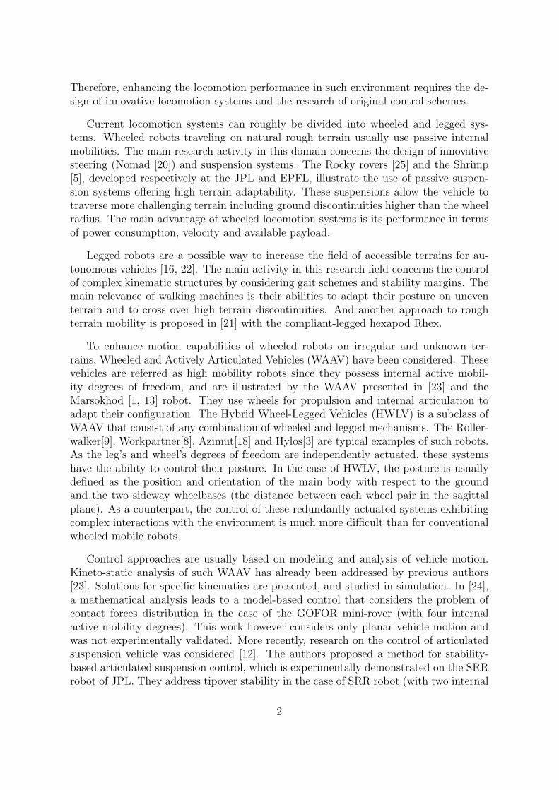
In this paper, we describe a solution that optimizes both the traction force balanceand the tipover margin for the Hylos robot, a high mobility redundantly actuated vehicledeveloped in the lab (see Figure 1). It is a lightweight mini-robot with 16 actively actu-ated degrees of freedom (four wheel-legs, each one combining a two degrees of freedomsuspension mechanism with a steering and driven wheel).

Figure 1: Hylos experimental prototype

The actuated degrees of freedom of this robot are split in two categories: the first oneconcerns the locomotion itself (traction and steering) and the second one the posture(orientation of the main body and sideway wheelbases). Thus, trajectory and posturecontrol will be treated together as they are coupled but specification of the desiredtrajectory and optimal posture p∗ will be considered separately. The posture controlalgorithm calculate the joint velocities q∗ to reach the desired posture p∗ and follow thedesired trajectory (see Figure 2). The number of posture parameters is related to thegeneral mobility index of the vehicle which depends on the number of internal activemobilities and, thus, on the particular design of the vehicle.

In the next section, we first develop the general kinetostatic model of a wheel-leggedvehicle. In Section 3, we define suitable locomotion criteria and address the postureoptimization problem, assuming quasi-static motion of the vehicle. However, due to theunderlying difficulty of on-line optimal posture computation, a suboptimal but compu-tationally efficient posture for the particular design of the Hylos robot is presented inSection 4 as well as a velocity based posture control algorithm. Finally, performance ofthe optimization process is analyzed through simulations of a wheel-legged vehicle onsloping terrain with various slope angles. The posture control algorithm is also evaluatedthrough simulations and experiments with the Hylos robot traveling on an irregular andsloping ground.

3

Trajectory specificationPosture control Posture

optimisation

Sensors

Criteria High mobility vehicle

p

p

q* *

Figure 2: General schematic of the controller

2 General formulation of kinetostatic model of wheel-

legged systems

This section deals with the development of the kinetostatic model for a general wheeledand articulated system. These models are used in Section 3 for load distribution opti-mization and in Section 4 for the vehicle posture control on rough terrain.

The considered system consists of a main body (platform S) connected to ser-ial articulated chains, each one terminated by a cylindrical wheel (Figure 3). DefineR=(G,x,y,z) a frame attached to the platform with G the platform center of gravity(c.o.g). The orientation of the platform frame is given by three angles with respect tothe fixed frame R0, which are the conventional yaw(θ)-pitch(ψ)-roll(ϕ) angles [4].

We assume that all wheels are in contact with the ground. Denote Pi the ith contactpoint and ni the normal vector to the tangent contact plane. The associated contactframe Ri = (Pi, ti, li,ni) is defined such as ti = σi×ni

||σi×ni||(σi is the ith wheel axis unit

vector) and li = ni × ti.

2.1 Velocity model

The velocity of each contact point Pi with respect to the ground can be written as:

v(Pi/R0) = v + ω × ri + v(Pi/R) (1)

where (v , ω)t = vp is the components vector expressing the twist of the platform andri the vector connecting the platform frame center G to contact point Pi.

The pure rolling condition at contact point Pi can be written as:

v(Pi/R0) = 0 (2)

The projection of this equation on contact frame vectors (ti, li,ni) provides differentphysical meanings:

4

ni

x

y

z

G

S

fi

Pi

r i

li

ti

Figure 3: General model of a wheel-legged vehicle

• titv(Pi/R0) = 0: expresses the non-slippage condition in the longitudinal direction,

• litv(Pi/R0) = 0: expresses the non-slippage condition in the lateral direction,

• nitv(Pi/R0) = 0: expresses the contact continuity condition.

With the pure rolling condition at contact point Pi, Equation (1) becomes:

−(v + ω × ri) = v(Pi/R) (3)

and its projection, in a matrix form, along the contact frame vectors yields to:

−(

Ri −RiS(ri))vp = Jiqi (4)

where Ri is the rotation matrix of the contact frame with respect to platform frame,Ji is the jacobian matrix of the ith wheel-leg chain with respect to the platform andexpressed in the contact frame, qi is the joint velocity vector of the wheel-leg chains,and S(u) is the skew-symmetric matrix of the cross product operator :

S(u) =

0 −u3 u2

u3 0 −u1

−u2 u1 0

Equation (4) can be written for each leg as:

Livp = Jiqi (5)

where Li is called the locomotion matrix of the ith wheel-leg chain.Finally, for all wheel-legs, we obtain:

L1

L2

...Ln

vp =

J1 0 0 00 J2 0 00 0 ... 00 0 0 Jn

q1

q2

...qn

(6)

5

or

L vp = J q (7)

2.2 Static model

We denote fi = (fti , fli , fni)t the contact force at point Pi expressed in the contact

frame Ri. The components of this contact force are called respectively the traction (orbraking) force, lateral force and normal force (or load). Equations of static equilibriumare obtained using the principle of virtual work. This gives, on the one hand, theequilibrium equation of the whole system:

Ltf = wt (8)

and, on the other hand, the contact force to joint’s torques τ mapping:

Jtf = τ + ws (9)

where f = (f1t, f2

t, .., fnt)t is the collection of all contact forces.

In these equations, wt is the components vector of the total wrench (expressed inthe platform frame) applied to the system and ws is the generalized force vector mainlydue to the weight of the different sub-parts of the system.

3 Posture optimization of wheel-legged vehicle

The locomotion performance of wheel-legged vehicles is directly related to the contactforces at each wheel-ground contact point. The allowable range of these contact forcesdepends on the vehicle posture. Thus, posture control in articulated ground vehicle is apossible way to enhance the locomotion performance. Controlling the posture can alsobe used to control the center of gravity position (i.e. the distribution of contact forces)and thus the tipover stability margin.

Estimation of contact forces is based on a quasi-static analysis of the vehicle con-figuration. Consider the high mobility locomotion system shown in Figure 3: it is ageneric model that represents both legged, wheeled and hybrid vehicle. The generickinematic model developed in Section 2 is used to find the optimal posture for thiswheel-legged vehicle. The resolution of forces distribution in closed-chain mechanismsis an underspecified problem [14]. With the assumption that the wheel-ground contactangles can be estimated [11, 2], the quasi-static equilibrium equation (Eq. (8)) gives theforce balance for a given configuration, using the pseudo-inverse of Lt.

6

3.1 Locomotion performance criteria

To find the posture vector p∗ that optimizes the vehicle locomotion performance, it isnecessary to select suitable evaluation criteria. In planetary exploration missions, funda-mental properties that should be enhanced are the vehicle reliability and its capacity totravel in difficult environment. Thus, in this paper, the mechanical stability margin (thesystem tipover limit) and the traction efficiency are considered to be the most suitableperformance criteria.

Stability criterion: The control of robotic systems under stability margin con-ditions was mainly addressed in the field of legged locomotion. Research on stabilitycontrol of walking machines was first considered in 1968 by McGhee and Frank [15]. Afirst static stability criterion was developed to evaluate the stability of an ideal machinewalking at constant speed on flat even terrain. It simply considers that the vehicle isstable if the projection of the center of gravity lies inside the support polygon. Differentmechanical stability margins were defined during past research on walking machines.They can be roughly split in three main categories [10]:

• the “Stability margin”[15] that evaluates the distance between the projection ofthe center of gravity and the support polygon,

• the “Gradient stability margin”[19] that evaluates the inclination angle of themachine at which it starts tumbling,

• the “Energy stability margin”[17, 6] that evaluates the difference between its max-imum potential energy and its initial one.

The control method presented in this paper considers the vehicle motion on irregularterrain without discontinuities. Thus, the tipover stability margin is mainly constrainedby terrain geometry. So, a ”Gradient stability margin” as the one proposed by Pa-padopoulos [19] is well adapted to our operational condition, as it integrates both thedistance of the projected c.o.g. to the support polygon and its vertical position rela-tively to the average plane defined by the contact points Pi. Furthermore, this methodis computationally efficient. It can be summarized as follow: the line joining two con-secutive terrain-contact points Pi define a tip-over axis. The unit vector hi of the axisjoining the vehicle c.o.g. G to the center of each tipover axis is computed. Then, angleθi between each hi and the total external force vector applied to the vehicle gives thestability angle over the corresponding tipover axis. The overall vehicle stability marginis defined as the minimum of all stability angles:

ms = min{θi, i = 1..n} (10)

When ms < 0, a tipover instability occurs.

Traction criterion: Consider the contact force fi = (fti , fli , fni)t as defined in

Section 2 and expressed in the local contact frame Ri. Denote ρi the ratio between

7

tangential and normal forces at each wheel-ground contact:

ρi =

√f 2li

+ f 2ti

fni

(11)

Traction efficiency is related to the slip that occurs at each wheel-ground contact. Re-ducing the potential for large-scale slippage is equivalent to minimize the maximumof each ratio ρi. The limit of controllability is reached when ρi ≥ fs, where fs is thewheel-terrain friction coefficient.

3.2 Formulation of the optimization problem

For a given set of posture parameters p (which depends on the particular design of thevehicle), the aim of the optimization process is to find the optimal posture vector p∗

which minimizes an objective function Φ.

The objective function Φ(p) can be expressed as a function of the locomotion per-formance criteria:

Φ(p) =n∑i=1

(Ks

θ2i

+Kρρ2i

)(12)

where ρi is a function of fi and θi a function of ri (vector connecting the c.o.g to eachcontact point), and Ks, Kρ are constant positive weighting factors. Minimizing thisfunction leads to maximize all the θi (i.e. the margin stability)and minimize all the ρi(i.e. the total vehicle slippage).

The vectors ri are computed as a function of p and the static equilibrium equation(Eq. (8)) is solved using the pseudo-inverse matrix to determine f :

f =(Lt

)+wt (13)

A standard conjugate gradient method could then be used to search for the optimalposture.

However, in order to evaluate the objective function, we need information aboutthe local terrain map to define the contact points Pi and the associated normal vectorsni. As the terrain map is generally unknown, Pi and ni have to be evaluated on line.Thus, the main drawback of this method lies on its practical issues: measurement ofthe contact normals and computational cost of the on-line optimization process. Thus,for the practical implementation of the posture control algorithm on the Hylos robot, asuboptimal solution is proposed in the next section.

8

4 Suboptimal posture definition and control of Hy-

los

In this section, we describe the method used for the posture control of Hylos robot. Weuse a proportional feedback control based on the inverse velocity model. We first define,through a kinematic analysis, the parameters of the posture vector p and then we givethe general inverse model used for both path tracking and posture control. Finally, wepresent the posture control algorithm applied to the Hylos robot as well as the definitionof a suboptimal posture for motion on slopes.

4.1 Hylos posture parameters definition

The number of posture parameters is related to the mobility of the vehicle which dependson the particular design of the Hylos robot. The mobility m is computed using theKutzbach form of Gruebler’s equation:

m =

j∑i=1

fi − 6(j − b+ 1) (14)

where b is the number of bodies, j is the number of joints and fi is the number offreedom for each joint.

Frontal plane

ly2G

Pix

xy

z

ri

ϕψ

gz

l1

l2

rω

lx2

i

Figure 4: Hylos kinematic model

The Hylos robot, presented in Figure 4, has a mobility m = 10 with 16 actuatedjoints: b = 18 (4 bodies for each leg, the platform and the ground), j = 20 (4 joints oneach leg and 4 wheel-ground contacts) and

∑fi = 28 (4 rotational joints for each leg

and 3 dof joints at each wheel-ground contact with ideal rolling constraint).

9

In the operational space, these mobilities are the 6 platform parameters vp and the4 wheelbase velocities xi of each contact. These parameters can be split into one part(vx, vy, ωz) dealing with the path tracking and the other (ωx, ωy, vz, x1, x2, x3, x4) withthe posture control. Then, the corresponding geometrical posture parameters are:

p = (ϕ, ψ, zg, x1, x2, x3, x4)t (15)

where :

• ϕ is the roll angle,

• ψ is the pitch angle,

• zg is the height of platform center of gravity relative to the ground and is defined

as the average of contact heights zi : zg =

∑i zi4

• xi is the wheelbase of each wheel.

4.2 Hylos inverse velocity model

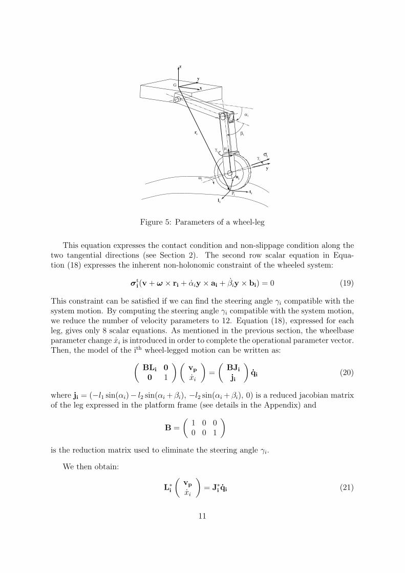
Let us consider the wheel-leg chain kinematics given in Figure 5: αi, βi are the leg’sjoint angles, γi the steering angle and ωi the wheel rate. Equation (3) expressed for theHylos robot becomes:

−(v + ω × ri) = αiy × ai + βiy × bi + γiµi × ci + ωiσi × di (16)

where µi,σi are the unit vectors of the steering and wheel axis, and ai, bi, ci, di thevectors connecting the joint axis to the contact point.

Due to the steering joint kinematics, the steering axis is almost perpendicular to thecontact surface. Then the cross product µi × ci = µi × −rwni is almost null whichmeans that the steering rate γi has no noticeable effect on the instantaneous motionof the platform. The normal vector is assumed to be in the wheel plane, then σi = liand ωi σi × di = ωi li × (−rwni) = −rwωiti. Assuming these conditions, Equation (3)becomes:

−(v + ω × ri) = αiy × ai + βiy × bi − rwωiti (17)

As in Section 2, this equation, projected in the ith contact frame, gives the followingmatrix form:

Livp = Jiqi (18)

where Ji = (y × ai y × bi − rwti) is the 3 × 3 jacobian matrix of each leg andqi = (αi, βi, ωi)

t.

10

σi

x

y

z

G

y

γ i

Pi

µ

β i

αi

i

γ i

ri

ωini

li

ti

Figure 5: Parameters of a wheel-leg

This equation expresses the contact condition and non-slippage condition along thetwo tangential directions (see Section 2). The second row scalar equation in Equa-tion (18) expresses the inherent non-holonomic constraint of the wheeled system:

σti(v + ω × ri + αiy × ai + βiy × bi) = 0 (19)

This constraint can be satisfied if we can find the steering angle γi compatible with thesystem motion. By computing the steering angle γi compatible with the system motion,we reduce the number of velocity parameters to 12. Equation (18), expressed for eachleg, gives only 8 scalar equations. As mentioned in the previous section, the wheelbaseparameter change xi is introduced in order to complete the operational parameter vector.Then, the model of the ith wheel-legged motion can be written as:(

BLi 00 1

) (vp

xi

)=

(BJi

ji

)qi (20)

where ji = (−l1 sin(αi)− l2 sin(αi +βi), −l2 sin(αi +βi), 0) is a reduced jacobian matrixof the leg expressed in the platform frame (see details in the Appendix) and

B =

(1 0 00 0 1

)is the reduction matrix used to eliminate the steering angle γi.

We then obtain:

L∗i

(vp

xi

)= J∗i qi (21)

11

Ji∗ is a 3x3 square matrix and can be inverted to give finally the wheel-leg motion

by:

qi = (J∗i )−1L∗

i

(vp

xi

)(22)

The projection of the non-holonomic constraint of Equation (19) in the vehicle frameR, gives the steering angle compatible with the vehicle motion (see details of this cal-culation in the Appendix):

γi = arctan

(v′iy

v′ix sin(αi + βi)− v′iz cos(αi + βi)

)(23)

where v′i = (v′ix , v

′iy , v

′iz) corresponds to: (v + ω × ri + αiy × ai + βiy × bi).

4.3 Posture control algorithm

For a given optimal posture p∗ and a desired trajectory, the goal of posture control is tocompute the internal joint velocities qi applied to each motor to maintain the optimalposture during the motion.

Let us introduce p = (ϕ, ψ, zg, x1, x2, x3, x4)t as the time derivative of posture

parameters. Then, the posture control is achieved by using a state feedback linearizingcontrol law:

p = Kp ∆p (24)

where ∆p = p∗−p is the posture error and Kp is a 7×7 diagonal positive gain matrix.The three other velocity parameters vt = (vx , vy , θ)

t are used in the trajectory trackingcontrol loop, which is not detailed in this paper.

The term zg is a function of vp (calculation details of this equation are given in theAppendix):

zg = −vt z +1

4

∑i

rit (S(ω)z) (25)

Since we have∑

i xi = 0 and∑

i yi = 0 for the suboptimal posture defined inSection 4.4, Equation (25) can be approximated as:

vz = −zg + ωy

∑i xi4

− ωx

∑i yi4

≈ −zg (26)

The platform angular velocities ω are coupled functions of (ϕ, ψ, θ)t. We introducethe coupling matrix D such as vp = D (vx, vy, vz, ϕ, ψ, θ)

t (see detail in the Appendix).This leads to the following matrix form for each leg:

vp = D (Cpp + Ctvt)xi = Cxi

p(27)

12

where Cp, Ct and Cxiare the corresponding component selection matrices.

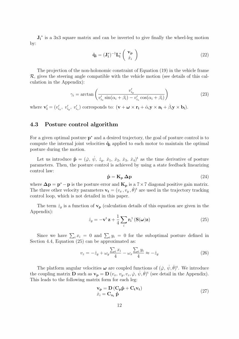
The joint velocities are computed from this operational velocity vector by consid-ering the inverse velocity model described in the previous paragraph. This model isbased on knowledge of the contact normal vectors ni. Equation (17) shows that ti canbe estimated from the measure of the absolute platform velocity (v,ω) and the leg’sjoint velocities (αi, βi). However, this estimation is theoretically independent from thewheel’s rotation rate ωi. For experimental tests, we use a simplified inverse velocitymodel which is based on a contact normal vector computed from the average plane ofcontact points Pi(xi, yi, zi).

Finally, the joint velocities are computed using Equation (22).

Figure 6: Posture control scheme

4.4 Suboptimal posture on slope

Due to the underlying difficulties of the on line optimization scheme presented at theend of Section 3, we here define a suboptimal posture for the motion of Hylos on slopingterrain.

From a static force distribution analysis, we can see that the stability margin andbalance of normal contact forces are optimal when the vertical component of the contactforces are equally distributed. It is well known that vertical contact forces balance can bereached by minimizing the projected distance, on horizontal plane, between the vehiclec.o.g and the geometric center of wheel-ground contacts. Moreover, this criterion alsooptimizes the traction force.

Since the gauge is constant for the particular design of Hylos, it is clear that thesideways force balance, in the front view, is obtained when the roll angle is zero ϕ = 0.The second constraint concerns a force balance in the sagittal plane between front andrear wheels. For a specified positive nominal wheelbase xn, the forces balancing criterionis verified if:

xi =xn

cos(ψ)− zg tan(ψ) (28)

13

where xn is the algebraic value of xn which is positive for the front wheels and negativefor the rear ones.

The vehicle ground clearance zg, the pitch angle ψ, and the nominal wheelbase xnare specified by the supervision control considering kinematic constraints on obstacleclearance and a constraint involving embedded scientific instruments. For example, itcould be necessary to keep the platform horizontal for vision-based measurements.

5 Results

In this section, we first present results showing an enhancement of the locomotion per-formance in terms of stability margin and traction, with the suboptimal posture formotion on sloping ground. We choose a constant ground clearance zg = −(l2 + rw) andpitch angle ψ = 0. The 5 other parameters of the posture vector are computed usingthe method presented in the previous section with a nominal wheelbase xn = lx + l1 (l1and l2 are the length of the leg links, lx is the half-length of the platform).

Next, simulation results show the ability of the posture control algorithm to ensurethe system stability on highly challenging terrains. Finally, experimental results for theposture control of Hylos moving on irregular terrain (consisting of a succession of slopeswith different inclination angles) show the feasibility of this method.

Furthermore, in order to illustrate the enhancement of Hylos locomotion perfor-mance, we purpose a comparison between the suboptimal posture configuration and thefixed-leg configuration. This configuration corresponds to a system without internal mo-bility degrees; i.e. with legs in a fixed position defined by: αi=cte=0 and βi=cte=−π/2.In the rest of this paper, the fixed-leg configuration will be referred to as the nominalposture.

5.1 Suboptimal posture on a sloping ground

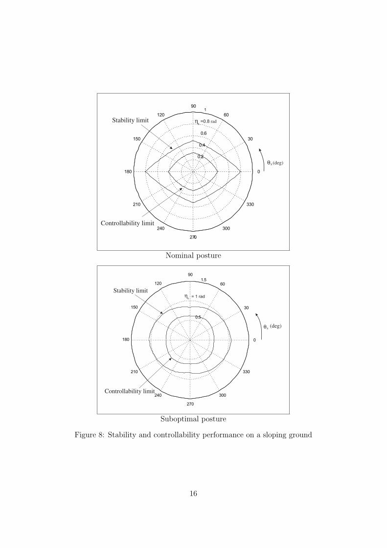
We denote ηs the maximum slope angle with respect to the horizontal plane and θs theheading angle of the robot x axis with respect to the line of maximum slope (see Figure7). Then, the corresponding pitch and roll angles of the robot in the rigid nominalposture are:

ϕ = arcsin (sin(θs) sin(ηs))ψ = arcsin (cos(θs) sin(ηs))

(29)

For each pair of angles (ηs, θs), the static model is solved for the suboptimal posturedefined above and for the rigid nominal posture. Then, we compute the stability limit(ms = 0) and the controllability limit (ρmax = fs), which is the limit when slippingoccurs.

14

G

xy

zθ

η

s

s

ϕψ

Figure 7: Slope angles definition

The stability and controllability limits are represented on a polar coordinate graphin Figure 8 with ηs for the radius and θs for the angle. Obviously, the stability andcontrollability domains are much larger for the suboptimal posture case. For the nominalposture, the stability and controllability are smaller for θs = π/2 as the gauge (vehiclewidth) is smaller than the wheelbase (vehicle length). When the suboptimal posture isconsidered, the stability limit is theoretically very important but is in practice mainlyconstrained by the operational workspace limit of each leg (|αi| < 50o, |βi| < 50o). Asthe roll angle is constrained to zero, we obtain an isotropic behavior of the controllabilitylimit curve.

5.2 Simulation results on posture control

In order to evaluate Hylos locomotion performance, we have developed a simulator[7] that takes into account the dynamics of wheel-legged robot and the wheel groundinteractions. The posture control algorithm presented in Section 4 has been implementedand evaluated for the Hylos robot traveling on irregular terrain (see Figure 9).

These simulations have the same initial and boundary conditions in terms of soilproperties and robot state. We specify a constant straightforward trajectory with avelocity of 30 cm/sec. The simulations were performed with suboptimal posture controland without posture control (constant nominal posture defined by αi = 0, βi = −π/2).The terrain used for these simulations is roughly irregular with two different surfaceprofiles in each sideways sagittal plane. It is a challenging terrain since without posturecontrol the system exhibits tipover instability.

The pitch and roll angles of the robot with posture control are plotted in Figure 10.This plot shows the performance of posture control for the selected feedback gain. Rollangles, which has the most important impact on the tipover margin, is well controlled,as the maximum error is less than 1o.

15

0.2

0.4

0.6

1

30

210

60

240

90

270

120

300

150

330

180 0

���

rad

(deg)

Stability limit

Controllability limit

θs

ηs =0.8

Nominal posture

0.5

1.5

30

210

60

240

90

270

120

300

150

330

180 0

= 1 rad

(deg)

Stability limit

Controllability limit

θs

ηs

Suboptimal posture

Figure 8: Stability and controllability performance on a sloping ground

16

Without posture controla tipover instability occurs

With posture controlthe system stability is insured

Figure 9: Simulation of Hylos motion

17

-5

-4

-3

-2

-1

0

1

2

3

4

5

times (s)

angl

es (d

eg)

Pitch and roll anglespitch angleroll angle

0 1 2 3 4 5 6 7 8 9 10

Figure 10: Pitch and roll posture control

In the Figure 11, the normal forces at each wheel-ground contact are represented,first in the case where the robot posture is not controlled (the fixed nominal posture)and secondly in the case where the robot is controlled to reach the suboptimal posture.The balance of normal forces is clearly improved in the second case. When the posturecontrol is used the maximum standard deviation is about 16 N against 42 N withoutposture control, which is an enhancement of around 40% of the normal force distribution.Furthermore, we notice that without posture control all the wheels are not kept incontact with the ground, whereas with supotimal posture control the minimal contactforce is higher than half the average normal force.

Last, evolution of the stability marginms during robot motion is plotted in Figure 12.We recall that this corresponds to the minimum of all tipover axis angles. It is computedfor both the case of suboptimal posture control and the case of fixed nominal posture.The mean stability margin of the system with posture control is 0.6 rad whereas it is0.15 rad with the rigid nominal posture. The minimum stability value is 0.5 rad usingposture control and is null in the other case as tipover instability occurs. This representsa significant enhancement of the system stability.

Thus, these simulation results show the feasibility of the posture control on irregularasymmetric terrain and demonstrate a significant gain in locomotion performance.

18

0 1 2 3 4 5 6 7 8 9 100

10

20

30

40

50

60

70

time (s)

f (N

)Normal force at each contact P (without posture control)

n

The leg 2 loose the contact with the ground

F 1F 2F 3F 4

nnnn

i

Average normal force

10

15

20

25

30

35

40

45

50

time (s)

f (N

)

Normal force at each contact P (with posture control)

n

i

F 1F 2F 3F 4

nnnn

0 1 2 3 4 5 6 7 8 9 10

Average normal force

Figure 11: Forces balance criterion

19

0

0.1

0.2

0.3

0.4

0.5

0.6

0.7

0.8Comparison of the stability margin

time (s)

m (

rad)

nominal posturesuboptimal posture

s

Robot tipover occur at this point

-0.10 1 2 3 4 5 6 7 8 9 10

Critical stability region

Figure 12: Stability margin criterion

5.3 Experimental results on posture control

The Hylos wheel-legged robot used for the experiments is approximately 60 cm longand weights 12 kg. It has four legs each combining a two degrees-of-freedom suspensionmechanism with a steering and driven wheel. Each leg is made of two 20 cm long linksdriven by two electrical linear actuators, and the wheel radius is 5 cm. This mechanismcan be seen as a large displacement active suspension. Hylos is equipped with a twoaxis inclinometer measuring the platform pitch and roll angles. One Motorola MPC555micro-controller is dedicated to the low-level control of the 16 actuators and a PC-104 board running RTLinux is used for the high-level posture control. Communicationbetween the PC and the micro-controller is achieved through a CAN bus.

The results presented in this section consider two experimental setups. The first iscomposed of two successive slopes and corresponds to a nominal sloping terrain. Thesecond is a more challenging one composed of two different terrain profiles in the left andright sagittal plane. This is an asymmetric terrain that involves a decoupled variationof the vehicle pitch and roll angles during its motion.

Experiments on slopes: In the first experiment, the robot moves straightforwardat a speed of 0.15 m/s with a constant heading angle θ = 38o on two successive slopes (seeFigure 13). Thus, both the pitch and roll angles must be controlled during the motion.The two main slope angles are 18o and 34o. The suboptimal posture is specified to bea null pitch and roll angles, with a constant ground clearance zg and the wheelbasescomputed from the method presented in Section 4.4.

20

Figure 13: First experimental setup - Terrain profile

-5

0

5

10

15

20

25

30

0 5 10 15 20 25 30 35 40

Angle (deg)

Time (s)

robot measured pitch angleslope pitch angle

-5

0

5

10

15

20

25

30

0 5 10 15 20 25 30 35 40

robot measured roll angle

Angle (deg)

Time (s)

slope roll angle

Figure 14: Experimental results of the posture control on slopes

21

In Figure 14, the dashed curves represent the vehicle pitch and roll angles whenposture control is active, and the solid curves is an estimate of the equivalent groundslope angles in pitch and roll directions. These angles correspond to the robot pitchand roll when it is moving with a fixed nominal posture and are computed with theEquation (29) defined in Section 5.1. The maximum error of the corrected angles (thepeak on each plot) is partially due to the response time of the feedback control (10 Hz)and partially due to the velocity limit of the leg’s actuators.

24° 6°

13°

24°

24°

360 cm

80 cm

(a) Terrain profil

(b) Hylos posture during motion

Figure 15: Second experimental setup

Experiments on irregular terrain: In the second experiment, the robot movesstraightforward at a speed of 0.08 m/s with heading angle θ = 0o on an asymmetricirregular terrain (Figure 15). The measured pitch and roll angles are plotted in Figure 16.We compare the measured angles in the rigid nominal posture to those when the systemis actively reconfigured around the suboptimal posture. These experiments show theability of the control algorithm to maintain a certain posture. The maximum deviationof pitch and roll errors are respectively 3o and 4o with posture control against 10o and30o without posture control (rigid nominal posture).

22

0 10 20 30 40 50 60- 40

- 30

- 20

- 10

0

10

20

30Robot pitch-roll angles (nominal posture without control)

time (s)

angl

e (d

eg)

rollpitch

0 10 20 30 40 50 60- 5

- 4

- 3

- 2

- 1

0

1

2

3

4

5Robot pitch roll angles (suboptimal posture with control)

time (s)

angl

e (d

eg)

rollpitch

Figure 16: Experimental results of the posture control on irregular terrain

23

6 Conclusion

In this paper, we have addressed posture control of hybrid wheel-legged vehicles. Asuboptimal solution that improves both the global traction and stability performancewas presented for the Hylos robot traveling on slopes.

Next, an original velocity-based posture control algorithm for a wheel-legged robothas been presented. This method is simple to implement as it needs only few sen-sors (a two axis inclinometer for the pitch-roll measurements and position sensors forthe leg mechanism). This algorithm has been validated through simulations showingthe capabilities of a vehicle to enhance its own stability in challenging environments.The practical feasibility of this control algorithm was evaluated and validated throughexperiments with the Hylos robot.

The next step in our work will be to study the force measurement at each wheel-ground contact point. These measurements will be useful for both on-line posture op-timization and posture control since knowledge of the wheel-ground contact forces is apossible way to estimate the ground contact angles required for the posture optimizationprocess. Further work will also deal with the dynamic stability control based on inertialmeasures for high obstacle clearance.

Appendix A: Decoupled kinematics

The rotation between platform frame and ground the frame is defined by the conven-tional yaw(θ)-pitch(ψ)-roll(φ) angles and is expressed by the following rotation matrix:

R =

CθCψ SθCψ −Sψ−SθCψ + CθSψSϕ CθCϕ + SθSψSϕ CψSϕSθSϕ + CθSψCϕ −CθSϕ + SθSψCϕ CψCϕ

(A-1)

In this case, the relation between platform rotation components ω and rotationparameters are:

ωx = ϕ− θ sinψ

ωy = ψ cosϕ+ θ cosψ sinϕ

ωz = θ cosψ cosϕ− ψ sinϕ

(A-2)

Then, we introduce the coupling matrix D such as vp = D (vx, vy, vz, ϕ, ψ, θ)t:

D =

I3×3 0

1 0 −Sψ0 0 Cϕ CψSϕ

0 −Sϕ CψCϕ

(A-3)

24

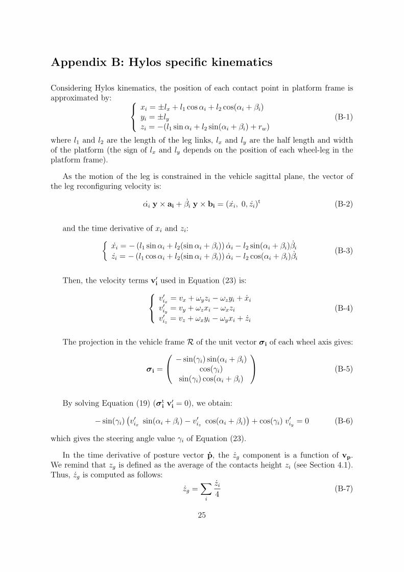
Appendix B: Hylos specific kinematics

Considering Hylos kinematics, the position of each contact point in platform frame isapproximated by:

xi = ±lx + l1 cosαi + l2 cos(αi + βi)yi = ±lyzi = −(l1 sinαi + l2 sin(αi + βi) + rw)

(B-1)

where l1 and l2 are the length of the leg links, lx and ly are the half length and widthof the platform (the sign of lx and ly depends on the position of each wheel-leg in theplatform frame).

As the motion of the leg is constrained in the vehicle sagittal plane, the vector ofthe leg reconfiguring velocity is:

αi y × ai + βi y × bi = (xi, 0, zi)t (B-2)

and the time derivative of xi and zi:{xi = − (l1 sinαi + l2(sinαi + βi)) αi − l2 sin(αi + βi)βizi = − (l1 cosαi + l2(sinαi + βi)) αi − l2 cos(αi + βi)βi

(B-3)

Then, the velocity terms v′i used in Equation (23) is:v′ix = vx + ωyzi − ωzyi + xiv′iy = vy + ωzxi − ωxziv′iz = vz + ωxyi − ωyxi + zi

(B-4)

The projection in the vehicle frame R of the unit vector σi of each wheel axis gives:

σi =

− sin(γi) sin(αi + βi)cos(γi)

sin(γi) cos(αi + βi)

(B-5)

By solving Equation (19) (σti v′

i = 0), we obtain:

− sin(γi)(v′ix sin(αi + βi)− v′iz cos(αi + βi)

)+ cos(γi) v

′iy = 0 (B-6)

which gives the steering angle value γi of Equation (23).

In the time derivative of posture vector p, the zg component is a function of vp.We remind that zg is defined as the average of the contacts height zi (see Section 4.1).Thus, zg is computed as follows:

zg =∑i

zi4

(B-7)

25

where zi = rit z.

The time derivative of zi is:zi = rt

i z + rit z (B-8)

where ri is the velocity of the contact point relative to the vehicle frame.

So, by considering the pure rolling condition introduced in Section 3 (non-slippingand contact constraints), this leads to:

ri = v(Pi/R0) − v(G/R0) = −v (B-9)

Since the time derivative of z vehicle frame vector is z = S(ω)z, we obtain:

zi = −vt z + rit (S(ω)z) (B-10)

And finally, the time derivative of zg is computed as follows:

zg = −vt z +1

4

∑i

rit (S(ω)z) (B-11)

References

[1] G. Andrade, F. BenAmar, Ph. Bidaud, and R. Chatila. Modeling wheel-sand in-teraction for optimization of a rolling-peristaltic motion of a marsokhod robot. InInternational Conference on Intelligent Robots and Systems, pages 576–581, 1998.

[2] J. Balaram. Kinematic state estimation for a mars rover. Robotica, 18(3):251–262,2000.

[3] F. BenAmar, V. Budanov, Ph. Bidaud, F. Plumet, and G. Andade. A high mobilityredundantly actuated mini-rover for self adaptation to terrain characteristics. In 3rdInternational Conference on Climbing and Walking Robots, pages 105–112, Madrid,Spain, 2000.

[4] J.J. Craig. Introduction to Robotics. Addison-Wesley, 1989.

[5] T. Estier, Y. Crausaz, B. Merminod, M. Lauria, R. Piguet, and R. Siegwart. Aninnovative space rover with extended climbing abilities. In International Conferenceon Robotics in Challenging Environments, Albuquerque, USA, 2000.

[6] A. Ghasempoor and N. Sepehri. A measures of machine stability for moving basemanipulators. In IEEE Int. Conference on Robotics and Automation, pages 2249–2254, 1995.

26

[7] Ch. Grand, F. BenAmar, P. Bidaud, and G. Andrade. A simulation system forbehaviour evaluation of off-road mobile robots. In 4th International Conference onClimbing and Walking Robots, pages 307–314, Germany, 2001.

[8] A. Halme, I. Leppanen, S. Salmi, and S. Ylonen. Hybrid locomotion of a wheel-legged machine. In International Conference on Climbing and Walking Robots,Madrid, Spain, 2000.

[9] S. Hirose and H. Takeuchi. Study on roller-walk (basic characteristics and itscontrol). In IEEE Int. Conference on Robotics and Automation, pages 3265–3270,1996.

[10] S. Hirose, H. Tsukagoshi, and K. Yoneda. Normalized energy stability marginand its contour of walking vehicles on rough terrain. In IEEE Int. Conference onRobotics and Automation, pages 181–186, 2001.

[11] K. Iagnemma and S. Dubowsky. Vehicle wheel-ground contact angle estimation:with application to mobile robot traction control. In Proceedings of the 7th Int.Symposium on Advances in Robot Kinematics, pages 137–146, 2000.

[12] K. Iagnemma, A. Rzepniewski, S. Dubowsky, and P. Schenker. Control of roboticvehicles with actively articulated suspensions in rough terrain. Autonomous Robots,14(1):5–16, 2003.

[13] A.L. Kemurdjian. Planet rover as an object of the engineering design work. In IEEEInternational Conference on Robotics and Automation, pages 140–145, Belgium,1998.

[14] V.R. Kumar and K.J. Waldron. Force distribution in closed kinematic chains. IEEEJournal of Robotics and Automation, 4(6):657–663, 1988.

[15] R. McGhee and A. Frank. On the stability properties of quadruped creeping gait.Mathematical Bioscience, 3:331–351, 1968.

[16] R.B. McGhee. Finite state control of quadruped locomotion. In Proceedings of theInternational Symposium on External Control of Human Extremities, 1966.

[17] D.A. Messuri and C.A. Klein. Automatic body regulation for maintaining stabilityof a legged vehicle during rough terrain locomotion. IEEE Journal of Robotics andAutomation, RA-1(3):132–141, 1985.

[18] F. Michaud and al. Azimut, a leg-track-wheel robot. In IEEE Int. Conference onIntelligent Robots and Systems, pages 2553–2558, 2003.

[19] E.G. Papadopoulos and D.A. Rey. A new mesure of tipover stability for mobilemanipulators. In IEEE Int. Conf. on Robotics and Automation, pages 3111–3116,1996.

27

[20] E. Rollins, J. Luntz, A. Foessel, B. Shamah, and W. Whittaker. Nomad: a demon-stration of the transforming chassis. In IEEE International Conference on Roboticsand Automation, pages 611–617, Belgium, 1998.

[21] U. Saranli, M. Buehler, and D.E. Koditschek. Rhex: a simple and highly mobilehexapod robot. Int. J. Robotics Research, 20:616–631, 2001.

[22] S.M. Song and K.J. Waldron. Machines that walk: the adaptative suspension vehi-cle. The MIT press, 1989.

[23] S.V. Sreenivasan and K.J. Waldron. Displacement analysis of an actively articu-lated wheeled vehicule configuration with extensions to motion planning on uneventerrain. Transactions of the ASME, 118(6):312–317, 1996.

[24] S.V. Sreenivasan and B.H. Wilcox. Stability and traction control of an activelyactued micro-rover. Journal of Robotics Systems, 11(6):487–502, 1994.

[25] R. Volpe. Rocky 7: A next generation mars rover prototype. Journal of AdvancedRobotics, 11(4):341–358, 1997.

28