Spontaneous synchrony in power-grid networks

Adilson E. Motter1,2,∗, Seth A. Myers3, Marian Anghel4 and Takashi Nishikawa1

Nature Physics 9, 191–197 (2013) | doi:10.1038/nphys2535

1Department of Physics and Astronomy, Northwestern University, Evanston, Illinois 60208, USA.2Northwestern Institute on Complex Systems, Northwestern University, Evanston, Illinois 60208,USA.3Institute for Computational and Mathematical Engineering, Stanford University, Stanford, Cali-fornia 94305, USA.4Information Sciences Group, Los Alamos National Laboratory, Los Alamos, New Mexico 87544,USA.

∗ E-mail: motter@northwestern.edu.

An imperative condition for the functioning of a power-grid network is that its power gener-ators remain synchronized. Disturbances can prompt desynchronization, which is a processthat has been involved in large power outages. Here we derive a condition under which thedesired synchronous state of a power grid is stable, and use this condition to identify tunableparameters of the generators that are determinants of spontaneous synchronization. Ouranalysis gives rise to an approach to specify parameter assignments that can enhance syn-chronization of any given network, which we demonstrate for a selection of both test systemsand real power grids. Because our results concern spontaneous synchronization, they arerelevant both for reducing dependence on conventional control devices, thus offering an ad-ditional layer of protection given that most power outages involve equipment or operationalerrors, and for contributing to the development of “smart grids” that can recover from fail-ures in real time.

1

arX

iv:1

302.

1914

v2 [

phys

ics.

soc-

ph]

1 M

ar 2

013

The current resounding interest in network synchronization1, 2 has been stimulated by theprospect that theoretical studies will help explain the behavior of real complex networks3. Re-cent advances include the modeling of chimera spatiotemporal patterns4, the discovery of low-dimensional dynamics in heterogeneous populations5, and the characterization of network syn-chronization landscapes6. However, despite the significant insights provided by these and otherstudies7–15, the connection between network theory and the synchronization of real systems re-mains under-explored. This is partly due to the scarcity of dynamical data, partly due to the ide-alized nature of the theoretical constructs (for network-unrelated exceptions, see refs. 16 and 17).In light of these considerations, we explore power-grid systems as genuine complex networks ofbroad significance that are amenable to theoretical modeling and whose dynamics can be simu-lated reliably. As the largest man-made machines in existence, modern power-grid networks oftenconsist of thousands of power substations and generators linked across thousands of kilometers.This complexity is reflected in a rich variety of collective behaviors and instabilities these systemsreportedly exhibit18.

Here, we focus on the synchronization of power generators—a fascinating phenomenon thatcan occur spontaneously, that keeps all connected generators in pace, and whose failure constitutesan important source of instabilities in power-grid systems. In a network of n alternating currentgenerators, a synchronous state is characterized by

δ1 = δ2 = · · · = δn, (1)

where δi = δi(t) represents the rotational phase of the ith generator and the dot represents thetime derivative. This synchronization frequency is assumed to be close (albeit not necessarilyequal) to a reference frequency. That coupled power generators can synchronize spontaneouslyis well known, as popularized in ref. 19, and this has generated recent interest in the physicscommunity20, 21. However, the governing factors and hence the extent to which this phenomenonmay occur in real power grids remain essentially unaddressed. Among the other studies that haveprovided substantive insights into power grid synchronization we mention the analysis of nonlin-ear modes associated with instabilities (refs. 22–24 and references therein) and of an equivalencebetween power systems and networks of nonuniform Kuramoto oscillators25–27. The former stud-ies provide an informative decomposition of nonlinear oscillations that arises when the networkloses synchrony. The latter studies establish a sufficient condition for a power grid to converge to asynchronous state, which is obtained via singular perturbation analysis from a similar condition fornonuniform Kuramoto oscillators25, 27. This condition is necessary and sufficient for non-identicaldynamical units under the assumption that the coupling strengths are uniform26. In contrast, the

2

stability condition we derive below is necessary and sufficient for heterogeneously coupled powergrids, with the assumption that a certain function of generator parameters is homogeneous. Thiscondition helps us address the question of how to strengthen synchronization.

Power grids deliver a growing share of the energy consumed in the world and will soon un-dergo substantial changes owing to the increased harnessing of intermittent energy sources, thecommercialization of plug-in electric automobiles, and the development of real-time pricing andtwo-way energy exchange technologies. These advances will further increase the economical andsocietal importance of power grids, but they will also lead to new disturbances associated withfluctuations in production and demand, which may trigger desynchronization of power generators.Although power grids can, and often do, rely on active control devices to maintain synchronism,the question of whether proper design would allow the same to be achieved while reducing de-pendence on existing controllers is extremely relevant. In the U.S., for example, data on reportedpower outages show that over 3/4 of all large events involve equipment misoperation or humanerrors among other factors28. This illustrates why stability drawn from the network itself would bedesirable.

The dynamics

We represent the power grid as a network of power generators and substations (nodes) connectedby power transmission lines (links). The nodes may thus consume, produce, and distribute power,while the links transport power and may include passive elements with resistance, capacitance, andinductance. The state of the system is determined using power flow calculations given the powerdemand and other properties of the system (see Methods), which is a procedure we implementfor the systems in Table 1. In possession of all variables that describe the steady-state alternatingcurrent flow, we seek to identify the conditions under which the generators can remain stablysynchronized.

The starting point of our analysis is the equation of motion

2Hi

ωR

d2δidt2

= Pmi − Pei, (2)

the so-called swing equation (ref. 29 and Methods), which, along with the power flow equations,describes the dynamics of generator i. The parameterHi is the inertia constant of the generator, ωRis the reference frequency of the system, Pmi is the mechanical power provided by the generator,and Pei is the power demanded of the generator by the network (including the power lost to damp-

3

ing). In equilibrium, Pmi = Pei and the frequency ωi ≡ δi remains equal to a common constant forall i, which is a sufficient condition for the frequency synchronization expressed in equation (1).

When the system changes because of a fault or a fluctuation in power demand, so does Pei.According to equation (2), immediately after the change the difference between the power de-manded and the power supplied by the generator is compensated by either increasing or decreas-ing the angular momentum from the generator’s rotor. The change in angular momentum does notremove the difference between Pei and Pmi; it only compensates for it until the spontaneous orcontrolled response of Pei and Pmi can adjust the r.h.s. of equation (2). It is through this processthat the generators can re-achieve the synchrony they may have lost in entering the transient state.But what are the properties of the network connecting the generators?

To address this question, we will first represent the power consumed at nodes of the networkas equivalent impedances30. This involves the assumption that the network structure is fixed andthe power demand is constant, which is appropriate because we are interested in the stability ofthe system on short time scales. For a given component, the corresponding admittance Y (thereciprocal of the impedance) is related to the voltage difference V and the complex conjugate ofthe power P through Y = P /|V |2. Thus, the admittances are usually complex.

The network structure

The admittance matrix Y0= (Y0ij) is defined analogously to the Laplacian matrix in oscillatornetworks: Y0ij is the negative of the admittance between nodes i and j 6= i, while Y0ii is the sumof all admittances connected to node i (the row sum is nonzero, however, due to finite impedancesto the ground). If V is the vector of node voltages and I is the vector of currents injected into thesystem at the nodes, then, according to the Kirchhoff’s law, I = Y0V. Because the non-generatornodes are now regarded as constant impedances, all nodes have zero injection currents except forthe generator nodes; this can be used to represent the effective interactions among the generatorsthrough a reduced network.

Indeed, rearranging Y0 such that the first n indices correspond to the generator nodes and theremaining r indices correspond to non-generator nodes, one has In

0

=

Y0n×n Y0n×r

Y0r×n Y0r×r

Vn

Vr

. (3)

4

The system is then converted to In = YVn by eliminating Vr, a procedure known as Kronreduction29, where the resulting effective admittance matrix is

Y = Y0n×n − Y0n×rY0−1r×rY0r×n. (4)

The existence of the matrix Y0−1r×r follows from the assumed uniqueness of the voltage vector V

(with respect to a reference voltage). In a system with n generators, the symmetric n × n matrixY defines a network in which generator nodes i and j 6= i are connected by a link of strengthdetermined by the effective admittance −Yij . The effective admittances are dominantly imaginary(the real part is smaller by up to one order of magnitude in the power grids we consider, as shownin Table 2). This indicates, as it will become clear below, that capacitances and inductances playan important role in the synchronization of generators.

The effective network connecting the generator nodes, represented by Y, is significantlydifferent from the physical network of transmission lines represented by Y0, as shown in Fig. 1 forthe power grid of Northern Italy. If the physical network is connected, as observed for this andany other system that we can treat as a single power grid, then the effective network will be fullyconnected31, meaning that any two generators are directly coupled through an effective admittance.This property of the effective network holds true under the assumption that the network is in asteady state, and is in contrast to the structure of the corresponding physical network, which istypically only sparsely connected. The connection strengths are not uniform in both the physicaland the effective network (Fig. 1). However, the distribution of weighted degrees (the sum of theabsolute values of all admittances connected to a node) is generally more homogeneous for Y thanfor Y0, as illustrated in Table 1 for several power networks. This degree homogeneity is a propertyof interest since it is known that it facilitates synchronization in networks of diffusively coupledoscillators32, 33. Surprisingly, as we show next, in power-grid networks this property can be lessdeterminant for synchronization than is the relation of certain generator parameters to the networkstructure.

The stability condition

To establish an interpretable relationship between synchronization robustness and power-grid pa-rameters, as well as to provide a condition that is necessary for any stricter form of stability,we focus on the short-term stability of the synchronous states under small perturbations. Wethus linearize equation (2) around an equilibrium (synchronous) state, associated with electricalpower P ∗ei and mechanical power P ∗mi and represented by δ∗i and ω∗i . Assuming that δi = δ∗i + δ′i,

5

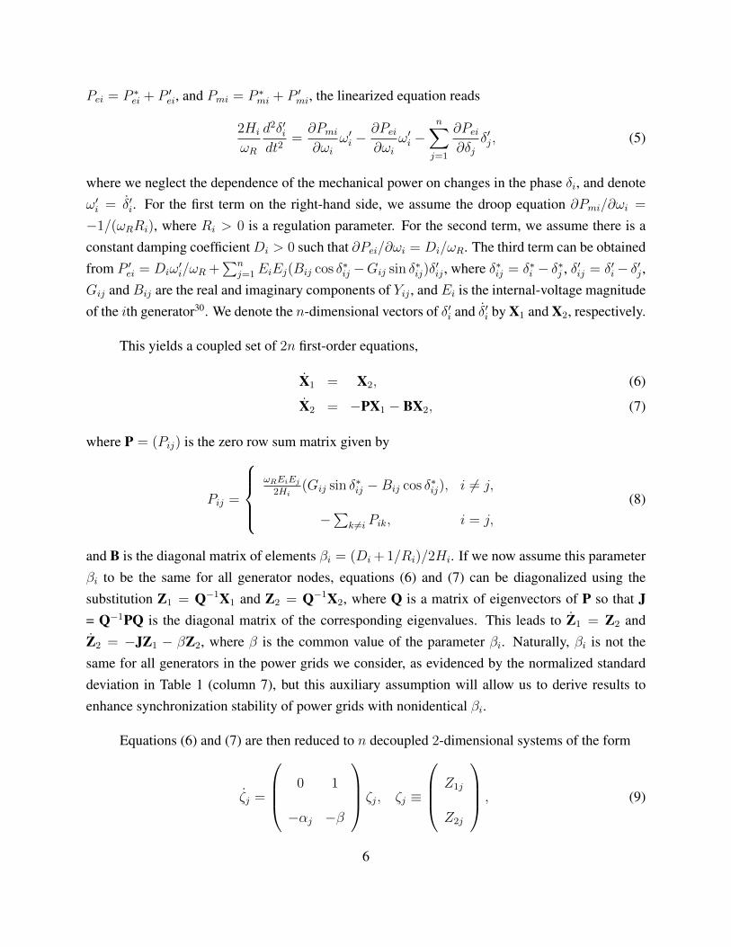
Pei = P ∗ei + P ′ei, and Pmi = P ∗mi + P ′mi, the linearized equation reads

2Hi

ωR

d2δ′idt2

=∂Pmi∂ωi

ω′i −∂Pei∂ωi

ω′i −n∑j=1

∂Pei∂δj

δ′j, (5)

where we neglect the dependence of the mechanical power on changes in the phase δi, and denoteω′i = δ′i. For the first term on the right-hand side, we assume the droop equation ∂Pmi/∂ωi =

−1/(ωRRi), where Ri > 0 is a regulation parameter. For the second term, we assume there is aconstant damping coefficientDi > 0 such that ∂Pei/∂ωi = Di/ωR. The third term can be obtainedfrom P ′ei = Diω

′i/ωR +

∑nj=1 EiEj(Bij cos δ∗ij −Gij sin δ∗ij)δ

′ij , where δ∗ij = δ∗i − δ∗j , δ′ij = δ′i− δ′j ,

Gij and Bij are the real and imaginary components of Yij , and Ei is the internal-voltage magnitudeof the ith generator30. We denote the n-dimensional vectors of δ′i and δ′i by X1 and X2, respectively.

This yields a coupled set of 2n first-order equations,

X1 = X2, (6)

X2 = −PX1 − BX2, (7)

where P = (Pij) is the zero row sum matrix given by

Pij =

ωREiEj

2Hi(Gij sin δ∗ij −Bij cos δ∗ij), i 6= j,

−∑

k 6=i Pik, i = j,

(8)

and B is the diagonal matrix of elements βi = (Di + 1/Ri)/2Hi. If we now assume this parameterβi to be the same for all generator nodes, equations (6) and (7) can be diagonalized using thesubstitution Z1 = Q−1X1 and Z2 = Q−1X2, where Q is a matrix of eigenvectors of P so that J= Q−1PQ is the diagonal matrix of the corresponding eigenvalues. This leads to Z1 = Z2 andZ2 = −JZ1 − βZ2, where β is the common value of the parameter βi. Naturally, βi is not thesame for all generators in the power grids we consider, as evidenced by the normalized standarddeviation in Table 1 (column 7), but this auxiliary assumption will allow us to derive results toenhance synchronization stability of power grids with nonidentical βi.

Equations (6) and (7) are then reduced to n decoupled 2-dimensional systems of the form

ζj =

0 1

−αj −β

ζj, ζj ≡

Z1j

Z2j

, (9)

6

where αj is the jth eigenvalue of the coupling matrix P. The matrix P always has a null eigenvalueassociated with a uniform shift of all phases, determined by X1 ∝ (1, . . . , 1)T , which correspondsto two perturbation eigenmodes (one for X2 = 0 and one for X2 = −βX1) that do not affectthe synchronization condition in equation (1). We denote this eigenvalue by α1 and exclude thecorresponding eigenmodes from subsequent analysis.

The stability of the synchronous state is governed by the Lyapunov exponents of system (9),

λj±(αj, β) = −β2± 1

2

√β2 − 4αj . (10)

The synchronous state is stable iff the real component of every Lyapunov exponent is negative forall j ≥ 2. That is, the stability condition translates to

max{±}

Reλj± ≤ 0, for j = 2, . . . , n. (11)

Because equation (9) is formally identical for all j, it is useful to drop the index j in equation (10)and define the function Λβ(α) = max{±}Reλ±(α, β) for fixed β and tunable parameter α. Thisfunction can be interpreted as a master stability function: the stability of the system is determinedby whether all the eigenvalues α2, . . . , αn fall within the negative region of Λβ . This stabilitycondition is of the form of those in refs. 34 and 35 for coupled oscillators, as explicitly shown inMethods.

The matrix P is generally asymmetric, meaning that the influence of a generator on anothergenerator is not necessarily identical to the influence of the second on the first. But we argue thatthe eigenvalues of P are all real over a range of conditions. We first factor the matrix as P = H−1P′,where H is the diagonal matrix of inertia constants Hi, to then note (inspired by a similar ar-gument in ref. 33) that the eigenvalues of P equal the eigenvalues of the partially symmetrizedmatrix P′′ = H−1/2P′H−1/2. The matrix P′′ is a zero row sum matrix of off-diagonal elementsωREiEj

2√HiHj

(Gij sin δ∗ij − Bij cos δ∗ij). We now observe that, due to the small real-to-imaginary com-

ponent ratio of the admittances and the predominance of small phase differences δ∗ij (Table 2), theantisymmetric part of P′′ is usually much smaller than the symmetric one; the 2-norm is over oneorder of magnitude smaller for the systems considered here, as shown in Table 3. If the eigenvaluesof the symmetric part of P′′, which are necessarily real, are nondegenerate (as generally observedin practice), then we can show that the eigenvalues remain strictly real in the presence of a smallantisymmetric component. Therefore, while our stability condition can be used in general, in whatfollows we will assume that P has real eigenvalue spectra, a condition observed to be satisfied inall of our simulations.

7

For real α, the stability region defined by Λβ(α) < 0 corresponds to α > 0. Indeed, thefunction Λβ is zero for α = 0 and becomes positive and increasingly larger for smaller α < 0;in the interval 0 < α ≤ β2/4, the function Λβ is negative and decreases as α increases. Forα > β2/4, the function Λβ is negative and remains constant since the radicand in equation (10) isnegative, rendering λj± to be complex. This behavior is summarized in Fig. 2a for different valuesof β, which further illustrates that varying β changes the behavior of the Lyapunov exponents asa function of α and, in particular, Λβ(α ≥ β2/4) = −β/2, but the stability condition that αj > 0

for all j ≥ 2 does not change. Moreover, for a given β > 0, the master stability condition does notdepend on whether this factor β is due to the presence of the regulation parameter Ri, the presenceof damping Di, or a combination of both. However, all other parameters left constant, both β andthe eigenvalues αj decrease as the inertia parameters Hi are uniformly increased. This has theeffect of reducing |Reλj± | and hence the strength of the linear stability or instability.

Enhancement of synchronization stability

We now apply this formalism to enhance the stability of the synchronous states by tuning theparameters of the generators. For βi = β, the synchronization stability is solely determined bythe master stability function Λβ(α) at α = α2, the smallest nonzero (real) eigenvalue of P. Thisfollows from the non-increasing dependence of Λβ(α) on α. For α2 > 0, which corresponds tostable synchronization, the quantity Λβ(α2) as a function of β attains its minimum at

β = βopt ≡ 2√α2 (12)

(see Fig. 2b). Given a network structure and a steady state, and hence a fixed value of α2, this pointof maximum stability can be achieved by adjusting one of the generator parameters.

Specifically, one can ensure that βi = βopt for all generators by adjusting the droop parameterRi to

Ri =1

4Hi√α2 −Di

, i = 1, . . . , n, (13)

or the damping coefficient Di to

Di = 4Hi

√α2 −

1

Ri

, i = 1, . . . , n, (14)

while keeping the other parameters unchanged. The tuning of the former, Ri, is most suitable foroff-line optimization of stability, since the time scales associated with this parameter30 are usuallylarger than those associated with typical instabilities. The latter,Di, can be adjusted dynamically at

8

very short time scales30 and hence is relevant for online optimization and fine-tuning under varyingoperating conditions that affect α2. Since equation (12) can be satisfied exactly, this approach leadsto the fastest possible asymptotic convergence rate to the synchronous state among all systems withthe same network structure and identical βi values.

More important, even when the βi values are not identical, as in the case of real power grids,adjusting Ri according to equation (13) or Di according to equation (14) in general results in sub-stantially improved stability. For example, consider the three test systems and the Guatemala powergrid in Table 1, which are all stable before any parameter adjustment. As these systems have non-identical βi values (Table 1, column 7), their stability was determined directly from equations (6)and (7) before diagonalization; the stability is quantified by λmax, the largest Lyapunov exponentexcluding the null exponent associated with the uniform shift of phases. A naive approach basedon parameter adjustment that homogenizes βi to their average β =

∑i βi/n does not necessarily

improve stability, as illustrated by the opposite effect observed in the Guatemala system (Table 1,columns 8 and 10). However, the adjustment to βopt improves stability in all systems, by a factorranging from 5 to nearly 90 in terms of λmax (Table 1, column 11).

This demonstrates that the mechanism by which synchronization stability can be enhancedrequires not only homogenization of the function βi of the generator parameters Hi, Di, and Ri,but also matching of this function with the structural and the dynamical state of the network rep-resented in α2. Furthermore, we can show that the maximum Lyapunov exponent λmax is locallyminimum at βi = βopt along any given direction in the βi-space for all systems we consider, whichis a necessary condition for this parameter assignment to be locally optimal for synchronizationstability. The approach is therefore appropriate for enhancing the stability of power networks forwhich the synchronous state is already stable. If the synchronous state is not stable, as in the caseof the Northern Italy and Poland systems for the dynamic parameters we consider, we can firstmake it stable by adjusting the generators’ transient reactances x′d,i (see Methods and Table 1, col-umn 9). Then, the synchronization stability can be further enhanced by the adjustment of βi toβopt, as illustrated in Fig. 3 for the Northern Italy system. Taken together, these results provide asystematic approach to strengthen stability in power-grid networks.

Discussion

Power grids are dynamic entities whose structure is history-dependent and evolves in a decentral-ized way that is often determined by market. The consequent difficulty to rationally design andmodify the network may be seen as a major limiting factor in optimizing synchronization in these

9

systems. Previous theoretical studies of synchronization in oscillator networks have shown that thestructure of the interaction network is a determinant factor for the dynamical units to synchronize2.In the most studied case of diffusively-coupled oscillators, it has been further shown that certainnetwork structures that inhibit synchronization can in fact facilitate synchronization when in pres-ence of other synchronization-inhibiting network structures, such as negative interactions6. But inpower grids, the relevant network is not simply the physical network of transmission lines, and thiscauses the structure and dynamics to be more intimately related than in such idealized models (seeMethods). In part because of this, here we have been able to show that the stability of synchronousstates in power grids can be enhanced by tuning parameters of the dynamical units rather than thenetwork.

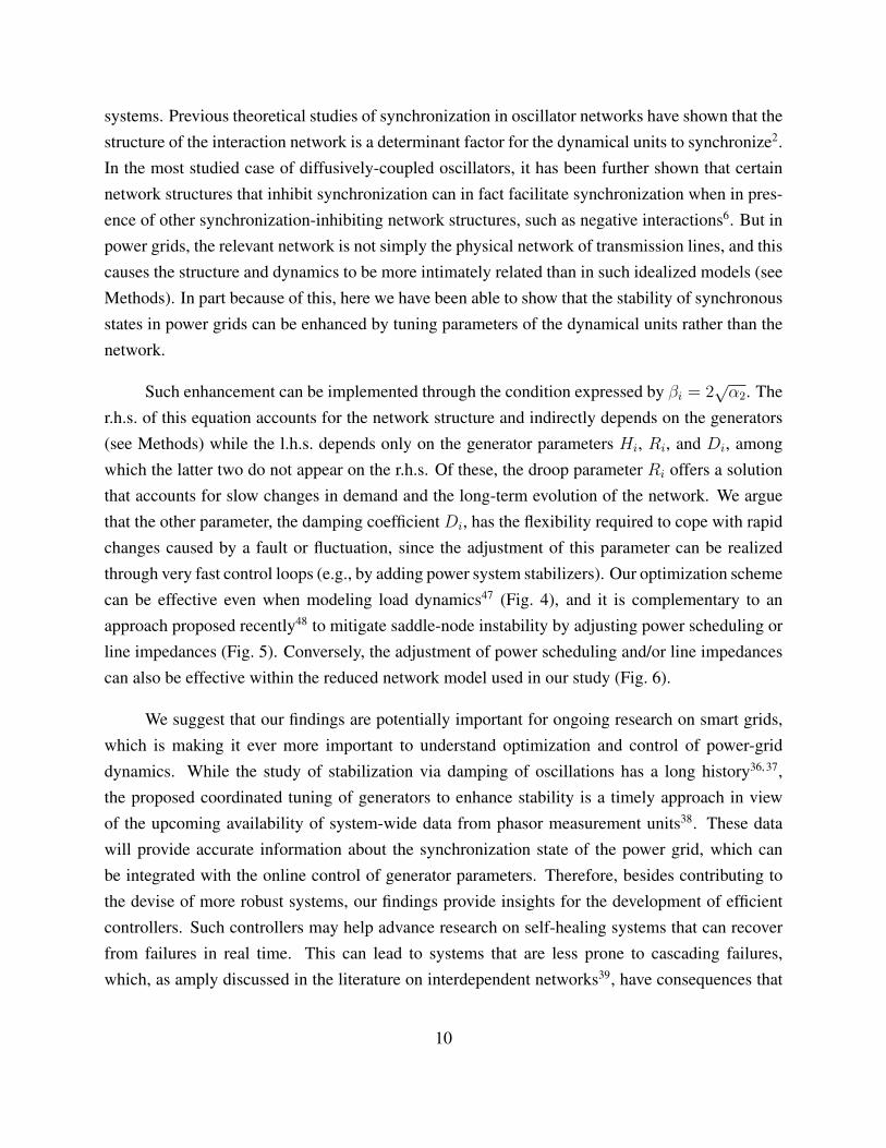
Such enhancement can be implemented through the condition expressed by βi = 2√α2. The

r.h.s. of this equation accounts for the network structure and indirectly depends on the generators(see Methods) while the l.h.s. depends only on the generator parameters Hi, Ri, and Di, amongwhich the latter two do not appear on the r.h.s. Of these, the droop parameter Ri offers a solutionthat accounts for slow changes in demand and the long-term evolution of the network. We arguethat the other parameter, the damping coefficient Di, has the flexibility required to cope with rapidchanges caused by a fault or fluctuation, since the adjustment of this parameter can be realizedthrough very fast control loops (e.g., by adding power system stabilizers). Our optimization schemecan be effective even when modeling load dynamics47 (Fig. 4), and it is complementary to anapproach proposed recently48 to mitigate saddle-node instability by adjusting power scheduling orline impedances (Fig. 5). Conversely, the adjustment of power scheduling and/or line impedancescan also be effective within the reduced network model used in our study (Fig. 6).

We suggest that our findings are potentially important for ongoing research on smart grids,which is making it ever more important to understand optimization and control of power-griddynamics. While the study of stabilization via damping of oscillations has a long history36, 37,the proposed coordinated tuning of generators to enhance stability is a timely approach in viewof the upcoming availability of system-wide data from phasor measurement units38. These datawill provide accurate information about the synchronization state of the power grid, which canbe integrated with the online control of generator parameters. Therefore, besides contributing tothe devise of more robust systems, our findings provide insights for the development of efficientcontrollers. Such controllers may help advance research on self-healing systems that can recoverfrom failures in real time. This can lead to systems that are less prone to cascading failures,which, as amply discussed in the literature on interdependent networks39, have consequences that

10

transcend the power grid itself.

Our analysis of power-grid dynamics also provides a fresh view of synchronization in com-plex networks in general. By identifying as the leading factor for stability the relation betweenthe specifics of the dynamical units and the network structure, it contrasts with most previousstudies, which focused on the role of the network structure alone (analyses of correlations be-tween the natural frequencies of phase oscillators and their connection topology are among thefew exceptions40–44). Aside from power grids and other technological applications, this is likelyto have implications for natural systems, such as biological ones, where the dynamical units co-evolve with the network structure45. Moreover, our analysis establishes a master stability conditionfor the synchronization of power generators, casting the problem in the framework of oscillatornetworks34 used to investigate collective behavior and nonlinear phenomena in a wide range ofcomplex systems. This facilitates comparison across different domains, and, we hope, will inspiresimilar developments on the tailoring of collective behavior in other real systems.

Methods

Power flow calculations and synchronous states. The power and voltage at each node weredetermined given the net injected real power and the voltage magnitude at each generator node,the power demand at each non-generator node, the reference voltage phase, the admittance of eachpower line, and the capacities of the network components. These power flow calculations wereperformed using the Power Systems Analysis Toolbox (PSAT)46. To identify the synchronousstates, the phase δ∗i of generator i was determined from the power and voltage at node i assumingthe classical model30. In this model, the generator is represented by a voltage source with constantmagnitude Ei and variable phase δi that is connected to the rest of the network through a transientreactance x′d,i and a terminal. Throughout the paper, we represent each generator and its terminalby a single node, except in the Kron reduction, where the terminals are treated as independentnodes to be eliminated.

Derivation of the swing equation. Equation (2) can be derived by setting the rate of change ofthe angular momentum of the rotor equal to the net torque acting on the rotor:

Jd2δidt2

= Tmi − Tei, (15)

where J is the moment of inertia in kg·m2, Tmi is the mechanical torque in N·m accelerating therotor, and Tei is the typically decelerating torque in N·m due to electrical load in the network.

11

Multiplying both sides by ωi and using the fact that the torque in N·m multiplied by the angularvelocity in radians per second gives the power in watts, the equation can be written in terms ofpower:

Jωid2δidt2

= Pmi − Pei. (16)

To make Pmi and Pei per unit quantities, we divide both sides of the equation by the rated power PR(used as a reference). The factor Jωi then becomes 2Hi/ωi, where we defined the inertia constantHi = Wi/PR (in seconds) and the kinetic energy of the rotor Wi = 1

2Jω2

i (in joules). Noting thatωi is approximately equal to the reference frequency ωR in systems close to synchronization, weobtain equation (2). A more detailed description of this derivation can be found in ref. 30 (secondedition, pp. 13–16).

Relation to the master stability formalism. Equations (6) and (7) when written individually foreach node i, can be expressed as

d

dt

δ′iδ′i

=

0 1

0 −βi

δ′iδ′i

+n∑j=1

Pij

0 0

−1 0

δ′jδ′j

. (17)

This is in the same general form as the variational equation for the class of coupled oscillatorsconsidered in ref. 34, which for a synchronous state s = s(t) is

d

dtxi = DF(s) · xi + σ

∑j

GijDH(s) · xj, (18)

where xi = F(xi) describes the node dynamics, H is the coupling function, and σGij representsthe strength of coupling from node j to i. The factors DF(s) and DH(s) in equation (18) are bothconstant matrices in equation (17), and Pij in equation (17) corresponds to σGij in equation (18),which are relations that can be used to derive Λβ(α) from equations (6) and (7) based on the resultsin ref. 34. Therefore, while the formalism in ref. 34 cannot be directly applied to equation (2), itcan be applied near the synchronization manifold, which is a procedure previously proposed for abroad class of coupled oscillators35.

Adjusting transient reactances for stability. We first observe that for Bij > 0, which is themost frequent case (Table 4), the cosine term in equation (8) is a destabilizing factor if |δ∗ij| >π/2. This instability often arises when a few specific generators have phases that are significantly

12

different from those of the other generators in the synchronous state, which can be due to thesegenerator’s transient reactance x′d,i. By identifying these generators through the negative sign ofthe corresponding diagonal elements of P and reducing their x′d,i, the instability can be suppressed.Applying this procedure to the Northern Italy and Poland networks indeed turns the systems stable(Table 1, column 9).

Relation between structure and dynamics. The interactions between generators in a power gridare in principle determined by the effective admittances, which are dominantly imaginary (Table 2).Thus, these interactions too have a sign; an inductive reactance (Bij > 0) suggests a positiveinteraction, and a capacitive reactance (Bij < 0) a negative one. However, it can be seen fromequation (8) that the interactions between the generators are in fact determined by Bij cos δ∗ij . Inorder for α2 > 0, as required for stable synchronization, the termsBij cos δ∗ij have to be dominantlypositive, as observed in real systems (Table 4). One can make any of these terms positive byhaving Bij and cos δ∗ij both positive or both negative, where having both factors positive is farmore common in real systems than both negative (Table 4). While Bij is mainly structural giventhe power flow solution, the parameter δ∗ij can be adjusted by changing specific properties of thegenerators, such as their transient reactances. Therefore, the interactions are in reality determinednot only by the network of effective admittances, but also by the system-level (alternate current)dynamics, which is in turn molded by the properties of the dynamical units. As a result, importantaspects in the network structure can be emulated by modifying tunable parameters of the dynamicalunits.

Power-grid data. The data required for power flow calculations were obtained as follows. Forthe 10-generator system, known as the New England test system, the parameters were taken fromref. 49. For the 3- and 50-generator systems, the parameters were taken from refs. 30 and 50,respectively. The data for the Guatemala and Northern Italy systems were provided by F. Milano(University of Castilla – La Mancha), and the data for the Poland system were provided as partof the MATPOWER software package51. The dynamic data required to calculate the synchronousstate, determine its stability, and simulate equation (2), are not all available for the real powergrids, and were obtained as follows. For all systems, we assumed that before any optimizationthe damping coefficient and droop parameter satisfy Di + 1/Ri = 50 per unit for all generators.The parameters x′d,i and Hi are available for the three test systems from the respective referencesmentioned above. For the Guatemala, Northern Italy, and Poland systems, we estimated x′d,i and

13

Hi using the strong correlation observed in the test systems between each of these parameters andthe power Pi injected by generator i into the network, as shown in Fig. 7. The estimated valuesare x′d,i ≈ 92.8P−1.3

i and Hi ≈ 0.04Pi, where Pi is in megawatts, x′d,i is in per unit, and Hi is inseconds.

References

1. Dorogovtsev, S. N., Goltsev, A. V. & Mendes, J. F. F. Critical phenomena in complex networks.Rev. Mod. Phys. 80, 1275–1335 (2008).

2. Arenas, A., Dıaz-Guilera, A., Kurths, J., Moreno, Y. & Zhou, C. Synchronization in complexnetworks. Phys. Rep. 469, 93–153 (2008).

3. Strogatz, S. H. Exploring complex networks. Nature 410, 268–276 (2001).

4. Abrams, D. M. & Strogatz, S. H. Chimera states for coupled oscillators. Phys. Rev. Lett. 93,174102 (2004).

5. Ott, E. & Antonsen, T. M. Low dimensional behavior of large systems of globally coupledoscillators. Chaos 18, 037113 (2008).

6. Nishikawa, T. & Motter, A. E. Network synchronization landscape reveals compensatorystructures, quantization, and the positive effect of negative interactions. Proc. Natl. Acad. Sci.

USA 107, 10342–10347 (2010).

7. Hagerstrom, A. M., Murphy, T. E., Roy, R., Hovel, P., Omelchenko, I. & Scholl, E. Experi-mental observation of chimeras in coupled-map lattices. Nat. Phys. 8, 658–661 (2012).

8. Tinsley, M. R., Nkomo, S. & Showalter, K. Chimera and phase-cluster states in populations ofcoupled chemical oscillators. Nat. Phys. 8, 662–665 (2012).

9. Assenza, S., Gutierrez, R., Gomez-Gardenes, J., Latora, V. & Boccaletti, S. Emergence ofstructural patterns out of synchronization in networks with competitive interactions. Sci. Rep.

1, 99 (2011).

10. Ravoori, B., et al. Robustness of optimal synchronization in real networks. Phys. Rev. Lett.

107, 034102 (2011).

11. Hunt, D., Korniss, G. & Szymanski, B. K. Network synchronization in a noisy environmentwith time delays: fundamental limits and trade-offs. Phys. Rev. Lett. 105, 068701 (2010).

14

12. Sun, J., Bollt, E. M. & Nishikawa, T. Master stability functions for coupled nearly identicaldynamical systems. Europhys. Lett. 85, 60011 (2009).

13. Yu, W., Chen, G. & Lue, J. On pinning synchronization of complex dynamical networks.Automatica 45, 429–435 (2009).

14. Kiss, I. Z., Rusin, C. G., Kori, H. & Hudson, J. L. Engineering complex dynamical structures:sequential patterns and desynchronization. Science 316, 1886–1889 (2007).

15. Restrepo, J. G., Ott, E. & Hunt, B. R. The emergence of coherence in complex networks ofheterogeneous dynamical systems. Phys. Rev. Lett. 96, 254103 (2006).

16. Strogatz, S. H., Abrams, D. M., McRobie, A., Eckhardt, B. & Ott, E. Crowd synchrony on theMillennium Bridge. Nature 438, 43–44 (2005).

17. Neda, Z., Ravasz, E., Brechet, Y., Vicsek, T. & Barabasi, A.-L. The sound of many handsclapping. Nature 403, 849–850 (2000).

18. Gellings, C. W. & Yeagee, K. E. Transforming the electric infrastructure. Phys. Today 57,45–51 (2004).

19. Strogatz, S. H. SYNC: The Emerging Science of Spontaneous Order (Hyperion, New York,2003).

20. Lozano, S., Buzna, L. & Dıaz-Guilera, A. Role of network topology in the synchronization ofpower systems. Eur. Phys. J. B 85, 1–8 (2012).

21. Rohden, M., Sorge, A., Timme, M. & Witthaut, D. Self-organized synchronization in decen-tralized power grids. Phys. Rev. Lett. 109, 064101 (2012).

22. Susuki, Y. & Mezic, I. Nonlinear Koopman modes and coherency identification of coupledswing dynamics. IEEE T. Power Syst. 26, 1894–1904 (2011).

23. Susuki, Y., Mezic, I. & Hikihara, T. Global swing instability in the New England power gridmodel. Proc. 2009 American Control Conference 3446–3451 (2009).

24. Parrilo, P. Model reduction for analysis of cascading failures in power systems. Proc. 1999

American Control Conference 4208–4212 (1999).

25. Dorfler, F. & Bullo, F. Synchronization and transient stability in power networks and non-uniform Kuramoto oscillators. Proc. 2010 American Control Conference 930–937 (2010).

15

26. Dorfler, F. & Bullo, F. On the critical coupling for Kuramoto oscillators. SIAM J. Appl. Dyn.

Syst. 10, 1070–1099 (2011).

27. Dorfler, F. & Bullo, F. Synchronization and transient stability in power networks and non-uniform Kuramoto oscillators. SIAM J. Control Optim. 50, 1616–1642 (2012).

28. NERC System Disturbances Reports 1992-2009. North American Electric Reliability Corpo-

ration (http://www.nerc.com).

29. Grainger, J. J. & Stevenson, W. D., Jr. Power System Analysis (McGraw-Hill Co., Singapore,2004).

30. Anderson, P. M. & Fouad, A. A. Power System Control and Stability, 2nd edition (IEEE Press -Wiley Interscience, Piscataway, 2003).

31. Dorfler, F. & Bullo, F. Spectral analysis of synchronization in a lossless structure-preservingpower network model. Proc. First IEEE International Conference on Smart Grid Communi-

cations 179–184 (2010).

32. Nishikawa, T., Motter, A. E., Lai, Y.-C. & Hoppensteadt, F. C. Heterogeneity in oscillatornetworks: are smaller worlds easier to synchronize? Phys. Rev. Lett. 91, 014101 (2003).

33. Motter, A. E., Zhou, C. S. & Kurths, J. Enhancing complex-network synchronization. Euro-

phys. Lett. 69, 334–340 (2005).

34. Pecora, L. M. & Carroll, T. L. Master stability functions for synchronized coupled systems.Phys. Rev. Lett. 80, 2109–2112 (1998).

35. Fink, K. S., Johnson, G., Carroll, T., Mar, D. & Pecora, L. Three coupled oscillators as a uni-versal probe of synchronization stability in coupled oscillator arrays. Phys. Rev. E 61, 5080–5090 (2000).

36. Gooi, H. B., Hill, E. F., Mobarak, M. A., Thorne, D. H. & Lee, T. H. Coordinated multi-machine stabilizer settings without eigenvalue drift. IEEE T. Power Ap. Syst. PAS-100, 3879–3887 (1981).

37. Dobson, I., et al. Avoiding and suppressing oscillations. PSerc Publication 00-01(http://www.pserc.wisc.edu, 1999).

16

38. Zhang, P., Chen, J. & Shao, M. Phasor Measurement Unit (PMU) Implementation and Appli-

cations (Electric Power Research Institute, Palo Alto, 2007).

39. Rinaldi, S. M., Peerenboom, J. P. & Kelly, T. K. Identifying, understanding, and analyzingcritical infrastructure interdependencies. IEEE Contr. Syst. Mag. 21, 11–25 (2001).

40. Brede, M. Synchrony-optimized networks of non-identical Kuramoto oscillators. Phys. Lett.

A 372, 2618–2622 (2008).

41. Carareto, R., Orsatti, F. M. & Piqueira, J. R. C. Optimized network structure for full-synchronization. Commun. Nonlinear Sci. 14, 2536–2541 (2009).

42. Buzna, L., Lozano, S. & Dıaz-Guilera, A. Synchronization in symmetric bipolar populationnetworks. Phys. Rev. E 80, 066120 (2009).

43. Kelly, D. & Gottwald, G. A. On the topology of synchrony optimized networks of a Kuramoto-model with non-identical oscillators. Chaos 21, 025110 (2011).

44. Gomez-Gardenes, J., Gomez, S., Arenas, A. & Moreno, Y. Explosive synchronization transi-tions in scale-free networks. Phys. Rev. Lett. 106, 128701 (2011).

45. Garlaschelli, D., Capocci, A. & Caldarelli, G. Self-organized network evolution coupled toextremal dynamics. Nat. Phys. 3, 813–817 (2007).

46. Milano, F. Power Systems Analysis Toolbox (University of Castilla – La Mancha, Ciudad Real,Spain, 2007).

47. Bergen, A. R. & Hill, D. J. A structure preserving model for power system stability analysis.IEEE T. Power Ap. Syst. PAS-100, 25–35 (1981).

48. Mallada, E. & Tang, A. Improving damping of power networks: Power scheduling andimpedance adaptation. IEEE Conference on Decision and Control and European Control Con-

ference 7729–7734 (2011).

49. Pai, M. Energy function analysis for power system stability (Kluwer Academic Publishers,Norwell, 1989).

50. Vittal, V. Transient stability test systems for direct stability methods. IEEE T. Power Syst. 7,37–43 (1992).

17

51. Zimmerman, R. D., Murillo-Sanchez, C. E. & Thomas, R. J. MATPOWER: Steady-state oper-ations, planning and analysis tools for power systems research and education. IEEE T. Power

Syst. 26, 12–19 (2011).

Acknowledgements The authors thank F. Milano for providing power-grid data, E. Mallada for sharing

unpublished simulation details, and F. Dorfler for insightful discussions. This work was supported by NSF

under Grants DMS-1057128 and DMS-0709212, the LANL LDRD project Optimization and Control The-

ory for Smart Grids, and a Northwestern-Argonne Early Career Investigator Award for Energy Research to

A.E.M.

Author contributions All authors contributed to the design of the research and analytical calculations.

S.A.M., M.A., and T.N. performed the numerical simulations. A.E.M. and T.N. wrote the paper, and A.E.M

supervised the project.

18

a b

Figure 1: Physical versus effective network for the power grid of Northern Italy. a, Rep-resentation of the physical network of transmission lines, which has 678 nodes and 822 links.b, Representation of the network of effective admittances, which is an all-to-all network with 170nodes corresponding to the generators in the system (a subset of the nodes in panel a). The colorscale of the lines indicates the link weights, ranging from yellow to red to black (scaled differ-ently for each panel), defined as the absolute value of the corresponding admittance. For clarity, inpanel b we show only the top 50% highest-weight links.

19

0

-1

-2

0 1 2

1

0

-1

0 1 2 3 4

Optimal

Stability region

a b

Figure 2: Stability of synchronous states for systems with βi = β. a, Real part of the Lya-punov exponents λ+ (continuous lines) and λ− (dashed lines) as functions of α for increasingvalues of β in the range 1.0–3.0. Although changing β causes changes in the shapes of Reλ±, theregion of stability defined by Λβ(α) < 0 is always α > 0. b, Real part of the Lyapunov exponentλ+ as a function of β, which has a minimum at β = 2

√α (illustrated here for α = 1). The stability

of synchronous states is maximum at this point.

20

t (sec) t (sec) t (sec)

a b dc

t (sec)

10-1

10-3

10-5

10-7

Figure 3: Enhancement of the stability of synchronous states. a–d, Response of the originalnetwork (a), the network with adjusted x′d,i (b), the network with βi = β (c), and the network withβi = βopt (d) to a perturbation in the Northern Italy power grid. The perturbation was applied tothe phase of each generator in the synchronous state at t = 0, and was drawn from the Gaussiandistribution with mean zero and standard deviation 0.01 rad. In each case, the network layout is thesame as in Fig. 1b and the bottom panel shows the time evolution of δ′i1 = δi1−δ∗i1, where δi1 is thephase of generator i relative to generator 1 and δ∗i1 is the corresponding phase in the synchronousstate. Generator 1, shown as a white node in the network, is used as a reference to discount phasedrifts common to all generators. The other nodes and their time-evolution curves are color-codedby the maximum value of |δ′i1| for 2 ≤ t ≤ 3. By adjusting the transient reactance of the generators,the divergence from the unstable steady state is converted to exponential convergence (a and b).This stability is improved upon adjusting the generator parameters to ensure a common value forβi, but is further improved when this common value is tuned to βopt = 2

√α2 (c and d).

21

0 2 4 6 8 100

2

4

6

8

10

1

2

3

4

5

6

7

Imp

rovem

en

t fa

ctor

Figure 4: Enhancement of synchronization stability in power-grid model incorporating loaddynamics. Colors indicate the factor by which the stability improves after adjusting all βi to thevalue βopt, where the darkest red corresponds to any factor > 7 and black to any factor < 1.The stability of a synchronous state is measured by the largest nonzero Lyapunov exponent λmax

computed within the Bergen-Hill model47. In this model, instead of eliminating non-generatornodes by the Kron reduction, load dynamics is modeled by assuming that the real power is a linearfunction of the voltage frequency for all power-consuming nodes, while the voltage magnitude isassumed to be constant for all nodes. For illustration, we use the 3-generator system studied in ref.48, with the power injection modified to Pi = 5, 6, 7 per unit. The improvement factor is shown asa function of the parameters Dgen and Dload, where Dgen is a coefficient given by (Di + 1/Ri)/ωR(assumed be the same for all generator nodes) and Dload is the frequency coefficient (assumedto be the same for all the other nodes). In most cases, our method yields significant stabilityimprovement, demonstrating its effectiveness beyond the reduced network model.

22

Figure 5: Combination of complementary approaches to mitigate instabilities associatedwith saddle-node bifurcations. As an example, we use the same 3-generator system described inthe caption of Fig. 4 with power injection Pi = 7.994, 3.006, 7.000, simulated using the Bergen-Hill model47. For Dgen = Dload = 1 per unit, the system is near a saddle-node bifurcation, andthus the Lyapunov exponent λmax is negative real and close to zero. At each iteration of the gradi-ent descent-like method described in ref. 48, which changes the power injected by the generators(independently of the values of βi and thus of Di), we compute λmax both with and without ad-justing βi to βopt by tuning the damping coefficients Di. The improvement factor, measured bythe ratio between the smallest λmax obtained through the iterative process with and without the βi-adjustment, is shown as a function of Dgen for different values of Dload. In most cases, significantadditional improvement results from the adjustment of βi, illustrating that near instabilities the twomethods can be combined to achieve enhancement not possible by either method alone. This re-sult is robust against heterogeneity in the network parameters, as illustrated in the inset histogramfor the system with Dgen = 0.5 and Dload = 1 (blue dot in the main plot), where each of thesecoefficients is independently perturbed according to the Gaussian distribution with mean zero andstandard deviation 0.1.

23

Iterations

Iterations

0 200 400 600 800 1000 1200−0.4

−0.2

0

0.2

0 600 1200

−0.1

0

0.1

0.2

Figure 6: Enhancement of synchronization stability via tuning of power injection withinthe reduced network model. We use the same 3-generator system as in Figs. 4 and 5, whereall system parameters are the same as in ref. 48, except for the power injection and consumption,which are initially set to 60% of the values used in that reference. This makes the system unstable,as indicated by the positivity of the Lyapunov exponent λmax for the synchronous state. The powerinjections were then adjusted iteratively according to the gradient descent-like scheme of ref. 48and λmax is plotted against the number of iterations for several values of the coefficient Dgen. In allcases, the power adjustment stabilizes the synchronous state, which is a consequence of increasingα2 across zero, as shown in the inset. Note that α2 is independent of Dgen because the synchronousstate in the reduced network model is unaffected by changes in Dgen.

24

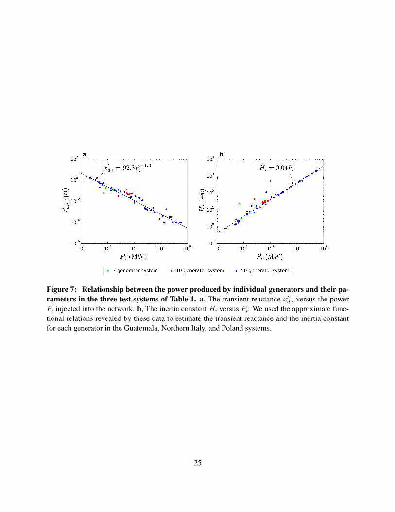
Figure 7: Relationship between the power produced by individual generators and their pa-rameters in the three test systems of Table 1. a, The transient reactance x′d,i versus the powerPi injected into the network. b, The inertia constant Hi versus Pi. We used the approximate func-tional relations revealed by these data to estimate the transient reactance and the inertia constantfor each generator in the Guatemala, Northern Italy, and Poland systems.

25

Table 1: Structural properties and synchronization stability of the systems considered.

System heterogeneity† Synchronization stability‡

System§ Nodes Links Generators Y0 Y βi Original x′d,i adjusted βi = β βi = βopt

3-generator test system 9 9 3 0.39 0.09 0.83 -1.71 — -2.21 -8.69

10-generator test system 39 46 10 0.81 0.38 0.37 -0.24 — -0.37 -3.65

50-generator test system 145 422 50 1.91 1.21 2.07 -0.02 — -1.53 -1.75

Guatemala power grid 370 392 94 6.86 1.18 1.22 -0.33 — -0.02 -4.19

Northern Italy power grid 678 822 170 3.42 0.84 2.02 7.20 -0.48 -1.59 -3.70

Poland power grid 2383 2886 327 2.26 3.00 0.92 140.07 -0.03 -0.02 -1.53

†As a measure of heterogeneity, we show the standard deviation normalized by the average. The quantities considered are the weighted degreescomputed for Y0 and Y, which represent the structure of the physical and effective network, respectively, and the parameter βi, which representsproperties of the generators. ‡As a measure of synchronization stability, we show the Lyapunov exponent λmax. We consider this exponent for theoriginal parameter values, for the transient reactance x′d,i adjusted, for all βi set equal to their average β, and for the generator parameter Ri and/orDi adjusted to ensure βi = βopt. §See Methods for a description of data sources.

26

Table 2: Phase difference in synchronous states and the real versus imaginaryparts of the admittances in the physical and effective networks.

Physical network† Effective network

System Mean |δ∗ij |/π Mean |G0ij | Mean |B0ij | Mean |Gij | Mean |Bij |

3-generator system 0.06 0.95 12.0 0.2367 1.275

10-generator system 0.07 6.81 80.9 0.3784 1.036

50-generator system 0.12 2.57 46.3 0.1978 1.242

Guatemala 0.08 7.74 62.1 0.0015 0.004

Northern Italy: original 0.07 105.88 758.3 0.0106 0.039

x′d,i adjusted 0.05 0.0104 0.042

Poland: original 0.25 24.06 597.3 0.0012 0.018

x′d,i adjusted 0.13 0.0013 0.019

†The real and imaginary components of the admittance −Y0ij are denoted −G0ij and −B0ij , respectively.

Table 3: 2-norm of the symmetric and antisym-metric parts of the matrix P′′.

System Symmetric Antisymmetric

3-generator system 0.68 0.011

10-generator system 0.48 0.018

50-generator system 1.89 0.016

Guatemala 3.04 0.085

Northern Italy: original 2.45 0.030

x′d,i adjusted 34.27 0.068

Poland: original 14.45 0.261

x′d,i adjusted 234.24 0.982

27

Table 4: Fraction of positive off-diagonal elements inthe matrices (Bij), (cos δ∗ij), and (Bij cos δ

∗ij).

System Bij cos δ∗ij Bij cos δ∗ij

3-generator system 1.000 1.000 1.000

10-generator system 1.000 1.000 1.000

50-generator system 0.689 0.995 0.687

Guatemala 0.999 1.000 0.999

Northern Italy: original 0.999 0.973 0.973

x′d,i adjusted 0.997 1.000 0.997

Poland: original 0.978 0.829 0.810

x′d,i adjusted 0.957 0.992 0.949

28