Spin-polarized Transport in Nanoelectromechanical Systems
96
Spin-polarized Transport in Nanoelectromechanical Systems Dissertation zur Erlangung des Doktorgrades an der Fakult¨ at f¨ ur Mathematik, Informatik und Naturwissenschaften Fachbereich Physik der Universit¨ at Hamburg vorgelegt von Jochen Br¨ uggemann Hamburg, 2015
Transcript of Spin-polarized Transport in Nanoelectromechanical Systems
Spin-polarized Transport inNanoelectromechanical Systems
Dissertation zur Erlangung des Doktorgrades
an der Fakultat fur Mathematik, Informatik und
Naturwissenschaften
Fachbereich Physik
der Universitat Hamburg
vorgelegt von
Jochen Bruggemann
Hamburg, 2015
Gutachter der Dissertation: Prof. Dr. Michael Thorwart
Prof. Dr. Jurgen Konig
Gutachter der Disputation: Prof. Dr. Daniela Pfannkuche
Prof. Dr. Michael Thorwart
Prof. Dr. Jurgen Konig
Prof. Dr. Hans Peter Oepen
Priv.-Doz. Dr. Peter Nalbach
Datum der Disputation: 01.06.2015
Vorsitzender des Prufungsausschusses: Prof. Dr. Daniela Pfannkuche
2
Abstract
In this work, the interplay between vibrational degrees of freedom and spin-polarized
charge transport on the nanoscale, induced by ferromagnetic charge reservoirs, is inves-
tigated. The dynamics of two different systems is determined by numerically solving
the Redfield master equation for the time-evolution of the reduced density matrix in
the sequential tunneling limit.
The first system is a proof-of-principle model for a dynamical cooling setup on the
nanoscale utilizing magnetomechanical interactions to reduce the vibrational energy of
a single phonon mode. The setup consists of a magnetic quantum dot tunnel-coupled
to a pair of ferromagnetic leads. Using spin-polarized currents, it is possible to polar-
ize the local magnetic moment of the quantum dot. Magnetomechanical interactions
then lead to an exchange of energy between the magnetic and vibrational degrees of
freedom, resulting in a decrease of the vibrational energy. The model is compared to
recent experiments to analyze its feasibility. The principle mechanism of the cooling
protocol is discussed and a meaningful initial preparation of the setup is found. The
spin and phonon dynamics of the system are analyzed for three different setups of the
lead polarization directions. An anti-parallel alignment of the source and drain lead
polarizations is identified as the optimal cooling setup due to an accumulation of spin
on the quantum dot. For a wide range of parameters a net cooling effect of the vibra-
tional mode is reported. A maximum of the cooling effect is found as a function of the
magnetomechanical coupling. This implies that cooling can be achieved not only for
strong magnetomechanical interactions.
The second system is an Anderson-Holstein model coupled to ferromagnetic leads.
Here, the differential conductance is determined as a function of the applied bias voltage.
The aim of this investigation is to explain experimental observations of the conductance
of a Cobalt-Phthalocyanine molecule in a scanning tunneling microscopy setup. The
numerical calculation of the conductance for the theory model is able to resolve the main
structure of the experimental data. A strong agreement is found for the position of the
conductance peaks with respect to the bias voltage. Discrepancies between the theory
and the experiment appear when the polarization of the microscope tip is reversed. The
change in peak intensities and positions observed in the experiment is not recovered
by a numerical calculation. These effects are assumed to originate from the magnetic
exchange field induced by the ferromagnetic leads. Due to the numerical restriction to
the sequential tunneling and, therefore, to weak system-lead couplings, a direct com-
3
parison of the influence of the exchange field between the experiment and the theory
model is not possible. In the last part of the thesis the effects of non-equilibrium and
equilibrium vibrations on the transport properties of the second system are evaluated.
A direct comparison shows that non-equilibrium distribution of the phonon mode leads
to a qualitative change in the transport dynamics only in the strong bias regime.
4

Kurzfassung
In dieser Arbeit wird das Zusammenspiel von vibronischen Freiheitsgraden und spin-
polarisiertem Ladungstransport auf der Nanoskala, induziert durch ferromagnetische
Zuleitungen, untersucht. Die Dynamik von zwei verschiedenen Systemen wird bestimmt
durch die Losung der Redfield Master Gleichung fur die Zeitentwicklung der reduzierten
Dichtematrix im sequentiellen Tunnellimit.
Das erste System ist ein Model fur einen Machbarkeitsnachweis eines dynamischen
Kuhlmechanismus auf der Nanoskala, der magnetomechanische Wechselwirkungen be-
nutzt, um die vibronische Energie einer einzelnen Phononenmode zu reduzieren. Das
Modell besteht aus einem magnetischen Quantenpunkt, der an ein Paar von ferromag-
netischen Zuleitungen gekoppelt ist. Durch die Nutzung von spin-polarisierten Stromen
ist es moglich, die lokale Magnetisierung des Quantenpunktes zu polarisieren. Mag-
netomechanische Wechselwirkungen resultieren dann in einem Austausch von Energie
zwischen den magnetischen und vibronischen Freiheitsgraden und dadurch in einer Ab-
nahme der vibronischen Energie. Das Modell wird mit aktuellen Experimenten ver-
glichen, um seine Realisierbarkeit zu uberprufen. Der grundlegende Mechanismus des
Kuhlprotokolls wird diskutiert und eine sinnvolle Praparation des Aufbaus wird gefun-
den. Die Spin- und Phononendynamik des Systems wird fur drei verschiedene Konfig-
urationen der Polarisierungsrichtungen der ferromagnetischen Zuleitungen analysiert.
Durch die Akkumulation von Spins auf dem Quantenpunkt stellt sich die anti-parallele
Ausrichtung der Polarisierungen der beiden Zuleitungen als optimale Konfiguration fur
das Kuhlen heraus. Ein Gesamtkuhleffekt der vibronischen Freiheitsgrade wird fur einen
grosen Parameterbereich gefunden. Dieser Kuhleffekt hat ein Maximum als Funktion
der magnetomechanischen Kopplung. Dies bedeutet, dass Kuhlung nicht nur fur starke
magnetomechanische Wechselwirkungen moglich ist.
Das zweite System besteht aus einem Anderson-Holstein Modell gekoppelt an ferro-
magnetische Zuleitungen. Die differentielle Leitfahigkeit wird als Funktion der Span-
nung ermittelt. Das Ziel dieser Untersuchung ist die Erklarung experimenteller Mes-
sungen fur die Leitfahigkeit von Cobalt-Phthalocyanine am Rastertunnelmikroskop. Die
numerischen Ergebnisse fur die Leitfahigkeit im Theorie-Modell spiegeln die Hauptstruk-
turen der experimentellen Daten wider. Es wird eine starke Ubereinstimmung fur die
Positionen der Spitzen in der differentiellen Leitfahigkeit gefunden. Unterschiede zwis-
chen der Theorie und dem Experiment treten auf, wenn die Polarisierung der Spitze des
Rastertunnelmikroskops umgekehrt wird. Die im Experiment beobachteten Anderungen
5
der Hohe und Position der Leitfahigkeitshochstwerte erscheinen nicht in der numerischen
Berechnung. Diese Effekte werden auf das Austauschfeld, welches von den ferromag-
netischen Zuleitungen induziert wird, zuruckgefuhrt. Aufgrund der Beschrankung der
numerischen Methode auf schwache System-Bad Kopplungen ist es nicht moglich, einen
direkten Vergleich fur den Einfluss des Austauschfeldes zwischen Theorie und Experi-
ment anzustellen. Im letzten Teil dieser Arbeit werden die Effekte von Gleichgewichts-
und Nichtgleichgewichtsvibrationen auf die Transporteigenschaften des zweiten Systems
untersucht. Ein direkter Vergleich zeigt, dass eine Nichtgleichgewichtsverteilung der
Phononenmode nur fur starke Spannungen zu einem qualitativen Unterschied in den
Transporteigenschaften fuhrt.
6
Contents
Contents
1. Introduction 9
2. Theoretical Background 15
2.1. Single-Electron Transport . . . . . . . . . . . . . . . . . . . . . . . . . . 15
2.2. Vibrational Sidebands and Spin-Polarized Currents . . . . . . . . . . . . 20
2.2.1. Franck-Condon Blockade . . . . . . . . . . . . . . . . . . . . . . 20
2.2.2. Spin-Polarized Currents . . . . . . . . . . . . . . . . . . . . . . . 22
2.3. Quantum Master Equation . . . . . . . . . . . . . . . . . . . . . . . . . 23
2.3.1. Derivation . . . . . . . . . . . . . . . . . . . . . . . . . . . . . . . 23
2.3.2. Redfield Master Equation . . . . . . . . . . . . . . . . . . . . . . 26
2.3.3. Diagrammatic Perturbation Theory . . . . . . . . . . . . . . . . 27
2.3.4. Numerical Solution . . . . . . . . . . . . . . . . . . . . . . . . . . 33
3. Cooling Nanodevices via spin-polarized Currents 35
3.1. Cooling Scheme . . . . . . . . . . . . . . . . . . . . . . . . . . . . . . . . 36
3.2. Model . . . . . . . . . . . . . . . . . . . . . . . . . . . . . . . . . . . . . 39
3.3. Energy Spectrum . . . . . . . . . . . . . . . . . . . . . . . . . . . . . . . 43
3.4. Principle mechanism . . . . . . . . . . . . . . . . . . . . . . . . . . . . . 45
3.5. Preparation . . . . . . . . . . . . . . . . . . . . . . . . . . . . . . . . . . 47
3.6. Effective Cooling . . . . . . . . . . . . . . . . . . . . . . . . . . . . . . . 50
3.7. Conclusion . . . . . . . . . . . . . . . . . . . . . . . . . . . . . . . . . . 62
4. Spin-polarized Transport through vibrating Molecules 65
4.1. Experiment . . . . . . . . . . . . . . . . . . . . . . . . . . . . . . . . . . 65
4.2. Model for spin-polarized magnetomechanical transport . . . . . . . . . . 69
4.3. Differential conductance and magnetomechanical molecular transport . . 71
4.4. Effective Field . . . . . . . . . . . . . . . . . . . . . . . . . . . . . . . . . 75
4.5. Non-equilibrium Phonon Mode . . . . . . . . . . . . . . . . . . . . . . . 78
4.6. Conclusion . . . . . . . . . . . . . . . . . . . . . . . . . . . . . . . . . . 81
5. Conclusion 83
A. Integral Kernels 85
7

8
1 INTRODUCTION
1. Introduction
The study of electronic devices on the micro- and nanoscale plays an important role
for the development of future technology. Both the memory capacity as well as the
operating speed of modern microelectronics depend on the size of the devices. Most
modern electronic hardware is composed of integrated circuits which contain arrays of
microtransistors. According to Moore’s law [1] the number of transistors per microchip
doubles roughly every eightteen months. By now, microchips have already reached
sizes of the order of tens of nanometers [2] and the process of miniaturization has
slowed down [3]. At this scale, also referred to as the nanoscale, quantum effects may
start to influence electronic transport properties. Macroscopic materials contain a large
number of particles. A mol of water, for example, weighs 18g and contains 6.022 · 1023
molecules. The physical properties of macroscopic materials measured in a laboratory
therefore are the result of an average over these large numbers of molecules rather than
their individual properties. In comparison, devices on the nanoscale contain a much
smaller number of molecules. Here, the individual behaviour of even a single molecule
can play an important role for the measurement of properties such as conductance or
heat capacity. Consequently, the investigation of quantum transport on the nanoscale
can become a vital component for the development of new technologies.
A particular example for the development of new devices on the nanoscale is the
molecular transistor [4, 5]. It consists of a single molecule in electrical contact with three
electrodes. By applying a bias voltage between two of the electrodes and a gate voltage
at the third electrode, it is possible to control the charge current flowing through the
molecule. In macroscale transistors the manipulation of the gate voltage can lead to an
increase or decrease of the current flowing through the transistor. Molecular transistors
exhibit a similar behaviour due to electron-electron interactions on the molecule. Strong
Coulomb interactions between the electrons can lead to a blockade of the charge current.
This concept is known as Coulomb blockade physics [6]. Molecules, however, do not only
possess electronic but also vibrational and magnetic degrees of freedom. Interactions
between these different degrees of freedom lead to new effects and open new possibilities
for the manipulation of electric currents.
A well-known effect of the interaction between electric and vibrational degrees of free-
dom is the Franck-Condon blockade [7–12]. Here, the coupling between the vibrational
motion and the number of charges on a nanodevice can lead to a suppression of the cur-
rent similar to the Coulomb blockade. Furthermore a signature of each vibronic state
9
of the system can be found in the current-voltage characteristics [13–17]. An example
of a system exhibiting such an effect is a quantum dot embedded in a nanoresonator.
Here, electrostatic forces between a gate electrode and electrons on the quantum dot
can cause a shift in the equilibrium position of the resonator. This shift in turn changes
the electronic transport properties of the device and induces a current blockade. Such
a phonon-induced current blockade can be enhanced further by driving the resonator
through a mechanical instability [18–21]. Consequently, nanoelectromechanical systems
(NEMS) can be used as sensitive detectors for displacement, charge or mass [22]. High
quality nanoresonators built of carbon nanotubes or SiO2 nanobeams are excellent con-
ductors. Their quality factors, given by the inverse eigenfrequency, can reach values of
the order of 105 [16, 17]. At sufficiently low temperatures these nanoresonators operate
in the deep quantum regime where zero-point fluctuations and other properties of quan-
tum mechanical motion could be detected. Further research on NEMS is also carried
out with the goal of information storage [23–25] by using molecular switches.
The development of new microscopic memory devices and qubits is also pursued in
the field of spintronics [26]. The field of spintronics is based on the study and manipula-
tion of electronic spins in solid state systems. Spin-polarized charge transport through
nanodevices can be induced by using ferromagnetic charge reservoirs. Ferromagnetic
materials exhibit a different density of states for electrons with different spin orienta-
tions. Consequently, applying a bias voltage to a set of ferromagnetic leads coupled to a
nanodevice induces a spin-polarized current. The influence of ferromagnetic leads on a
nanodevice can be expressed in terms of an effective magnetic field [27–31]. Combining
this effect with internal magnetic degrees of freedom of nanodevices has lead to the
possibility to construct spin filters or spin valves [32, 33]. A non-collinear orientation of
the lead polarizations and external magnetic fields leads to interesting phenomena such
as a negative differential conductance as a result of spin accumulation and precession
on the nanodevice [28].
While both the Franck-Condon blockade as well as spin-polarized charge transport
have been investigated in detail individually, a combination of these two effects has
so far not been studied. The focus of this thesis is to combine these two effects and
investigate spin-polarized charge transport in nanodevices with vibrational degrees of
freedom.
Direct interactions between magnetic degrees of freedom and vibrations, in form of
heat, are also investigated in the field of spin caloric transport [34]. Here, effects such as
the Spin-Seebeck effect [35] are analyzed in order to understand the interplay between
10
1 INTRODUCTION
spin and heat-based transport phenomena. Such an understanding is also of importance
for the development of new cooling techniques for micro- and nanodevices. Sending a
current through a microchip inevitably leads to Ohmic heating. Many modern devices
rely on passive cooling mechanisms in order to remove the produced heat. Commonly,
heat is transferred to the environment via a thermal contact between the nanoelectrical
device and its supporting structure. The efficiency of such passive heating mechanisms
however is limited. The demand for larger processing powers and the increasing number
of transistors per microchip will eventually lead to a heating problem. A solution can be
found by active cooling protocols. Such active or dynamical cooling mechanisms could
also further reduce the size of electronic devices by removing the necessity for spacious
cooling equipment. One example for such a nanorefrigerator is the idea to remove heat
via an electronic charge current [36, 37].
In this thesis, we propose and analyze a novel cooling mechanism on the nanoscale
based on magnetic degrees of freedom [38, 39]. In analogy to the macroscale demagneti-
zation cooling [40], we utilize the exchange of energy between magnetic and vibrational
degrees of freedom. More accurately, we analyze the spin and phonon dynamics of a
magnetic quantum dot with vibrational degrees of freedom coupled to a set on non-
collinearly polarized ferromagnetic leads. Applying a bias voltage between the ferro-
magnetic leads induces a spin-polarized charge current through the quantum dot. This
current leads to a polarization of the localized magnetic moment of the quantum dot.
Energy exchange between the magnetic and vibrational degrees of freedom then leads
to a decrease in the vibrational energy of the device. Simultaneously the charge cur-
rent gives rise to Ohmic losses which produce heat. Our investigation shows that it is
possible to prepare the setup in such a way that the cooling due to magnetomechanical
exchange can overcome the Ohmic heating effects leading to an overall effective cooling
of the device. A molecular magnet embedded on a suspended carbon nanotube attached
to ferromagnetic charge reservoirs could constitute an experimental realization of our
theory model. Here, experimentalists have already found a clear signature of magne-
tomechanical interaction [41]. Similar effects have been reported for nitrogen vacancies
coupled to a SiC cantilever [42, 43].
A different use of spin-polarized currents on the nanoscale can be found in spin-
resolved spectroscopy. The investigation and development of single molecule transis-
tors requires knowledge of the electronic, mechanical and magnetic properties of the
molecule. The energy spectrum of such a molecule can be detected by spectroscopic
methods such as scanning tunneling microscopy. The preparation of measurement sam-
11
ples however often leads to a hybridization of the molecules. This changes exactly those
properties which we want to investigate. Recent studies therefore prepare molecules on
insulating substrates in order to avoid hybridization [44–47]. In order to understand the
resulting experimental findings, we investigate spin-polarized transport in an Anderson-
Holstein model [48, 49]. A comparison between the experimental and theoretical data
shows a strong influence of the ferromagnetic leads. The effective field formed by the
lead polarizations, however, depends on the electronic energy levels which are shifted by
the electron-phonon interaction. Strong electron-phonon couplings can therefore lead
to a significant change of not only the electronic but also the magnetic properties of
the system. These observations indicate that a negative differential conductance or a
Kondo-effect [50] could be induced or enhanced by the vibrational degrees of freedom.
For our calculations of the system dynamics for both the nanorefrigerator and the
Anderson-Holstein model we rely on a numerical solution of the master equation. A
quantum master equation describes the time evolution of an open quantum system
under the influence of an environment such as the ferromagnetic leads used in both
models. Numerical solutions for the quantum master equation can be found for exam-
ple by using the quasi-adiabatic path integral formalism (QUAPI)[51–54]. In QUAPI
the time evolution of the system is formulated using a path integral. The influence of
the environment can then be integrated out and is contained in the so-called influence
functional [55]. Depending on the size of the system such a solution for an exact master
equation can be numerically very demanding and lead to long calculation times. The
same restrictions apply for a direct integration of the master equation or stochastic
methods such as Monte-Carlo simulations. In this thesis, we focus on the regime of
weak system-bath interactions and Markovian dynamics. Under these two assumptions
the master equation can be transformed into a Redfield master equation. A numerical
solution of the Redfield equation can be found by solving the eigenvalue problem for the
Redfield tensor. This method is significantly faster than the previously mentioned meth-
ods. Methods based on the Redfield equation have been successfully used to investigate
transport on the nanoscale [56] including both spin-polarized transport [28, 30, 31] as
well as phonon-assisted transport [57, 58] or the calculation of heat currents in quantum
refrigerators [59].
The thesis is structured as follows. In Chapter 2 we give an overview over Coulomb
blockade physics in single-electron transistors and provide a brief summary of preex-
isting literature explaining fundamental effects which reappear in the course of the
thesis. We then establish the numerical framework for our calculations by deriving the
12
1 INTRODUCTION
quantum master equation for open quantum systems in the limit of weak system-bath
interactions. Chapter 3 is designated to our main results. We develop a dynamic cool-
ing protocol for a magnetic nanodevice and set up a model for a proof-of principle of
the nanocooling scheme. By investigating the spin and phonon dynamics of the model
we show that an effective cooling of the vibrational degrees of freedom is possible for
a wide range of parameters. An investigation of the influence of ferromagnetic leads
on charge transport through molecules can be found in Chapter 4. Here, we compare
recent experimental findings to a theory model and provide a qualitative explanation
by analytic determination of the polaronic shift and the effective magnetic field of the
leads. Finally, we give a summary and conclusion of our results in Chapter 5.
13

14
2 THEORETICAL BACKGROUND
2. Theoretical Background
In this chapter we describe the fundamental physical principles and theoretical tools
which appear in this thesis. We start by explaining single-electron transport and
Coulomb blockade physics using the example of the single-electron transistor in Sec-
tion 2.1. Based on the conclusions of this example we review literature on the influence
of vibrational and magnetic degrees of freedom on quantum transport in Section 2.2.
Our goal is to study a combination of these effects. In order to so we derive a master
equation for the time evolution of the density matrix of an open quantum system in Sec-
tion 2.3. Knowledge over the time evolution of our model system allows us to determine
transport properties and the dynamics of electrons, vibrations and spins. We discuss
the Redfield approach and diagrammatic perturbation theory as tools for solving the
master equation and describe the numerical procedure to obtain a solution.
2.1. Single-Electron Transport
The study of mesoscopic or nanosystems often deals with nonequilibrium transport
properties. Such properties are also the focus of this thesis. More specifically, we
want to investigate spin-polarized transport in nanodevices. For this, we first need to
understand the basic principles of charge transport on the nanoscale. Let us start with
a quantum system on the nanoscale coupled to an electronic environment. Such an
environment can be provided for example by the macroscopic leads of a nanoelectronic
device. These leads act as charge reservoirs and the interaction with the system allows
charge carriers, the electrons, to tunnel between the system and the leads. Let us
further assume that the coupling between the nanodevice and the leads is weak. The
average life-time of a charge state on the nanodevice then is quite long. Changing the
state is only possible via a transfer of electrons to or from the leads. The probability
for such a charge transfer is directly proportional to the coupling strength between
leads and system. Specifically a simultaneous occurrence of several charge transfers is
very unlikely for weak couplings. As such the elementary physics of the device can
be explained by the rather simple mechanism of single-electron transfers. The most
prominent example for such a system is the single-electron transistor [6]. Realizations
of such devices can be found in form of single molecules [4, 5] or artificially produced
quantum dots [60]. In the following we want to provide a qualitative understanding of
the behaviour of single-electron devices in the presence of Coulomb interactions.
A single-electron transistor (SET) is the nanoscale equivalent of a classical transistor.
15
2.1 Single-Electron Transport
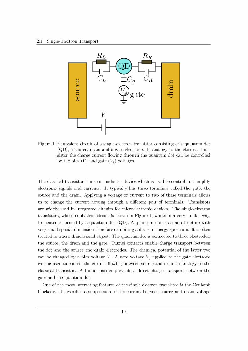
Figure 1: Equivalent circuit of a single-electron transistor consisting of a quantum dot(QD), a source, drain and a gate electrode. In analogy to the classical tran-sistor the charge current flowing through the quantum dot can be controlledby the bias (V ) and gate (Vg) voltages.
The classical transistor is a semiconductor device which is used to control and amplify
electronic signals and currents. It typically has three terminals called the gate, the
source and the drain. Applying a voltage or current to two of these terminals allows
us to change the current flowing through a different pair of terminals. Transistors
are widely used in integrated circuits for microelectronic devices. The single-electron
transistors, whose equivalent circuit is shown in Figure 1, works in a very similar way.
Its center is formed by a quantum dot (QD). A quantum dot is a nanostructure with
very small spacial dimension therefore exhibiting a discrete energy spectrum. It is often
treated as a zero-dimensional object. The quantum dot is connected to three electrodes,
the source, the drain and the gate. Tunnel contacts enable charge transport between
the dot and the source and drain electrodes. The chemical potential of the latter two
can be changed by a bias voltage V . A gate voltage Vg applied to the gate electrode
can be used to control the current flowing between source and drain in analogy to the
classical transistor. A tunnel barrier prevents a direct charge transport between the
gate and the quantum dot.
One of the most interesting features of the single-electron transistor is the Coulomb
blockade. It describes a suppression of the current between source and drain voltage
16
2 THEORETICAL BACKGROUND
due to strong Coulomb repulsion between electrons on the quantum dot. Many solid
state systems have been found to be described surprisingly well within models which
neglect electron-electron interactions. Since most of those are many-body systems a full
description including such interactions presents an unsolvable problem. To understand,
however, experiments on quantum dots these interactions can not be neglected. The
small spatial confinement formed by the quantum dot leads to a quantization of the
energy spectrum and gives rise to Coulomb repulsion between electrons trapped on the
dot. Let us assume that the quantum dot is a point-like structure containing n electrons
with charge e. The energy needed to add another electron to the dot is then given by
E =e2
2CΣn2 = ECn
2, (1)
where EC = e2/2CΣ is the charging energy, CΣ = CL+CR+Cg the total capacitance of
the single-electron transistor and CL, CR and Cg are the capacitances of the source, drain
and gate electrode, respectively. As mentioned earlier, the SET can be manipulated by
changing the gate and bias voltages. The influence of the electrodes can be expressed
as an induced charge q = CRVR+CLVL+CgVg, where VL, VR denote the potential shift
for the source and drain electrode. Notice that the induced charge q is not the charge of
a particle and therefore, in contrast to the charge transfer from and to the quantum dot
or its occupation number, is not a quantized number. We can then express the energy
level of the quantum dot as a function of its occupation number n as
E(n) = EC(n− q/e)2. (2)
Assuming that the quantum dot has no other internal degrees of freedom we have now
knowledge of its energy spectrum depending on the number of electrons on the dot
and the interaction with the electrodes. Our goal is to discuss single-electron transfers
between the quantum dot and the electrodes. A finite current only appears if there is
a preferred direction of charge transfer. It can be induced by applying a bias voltage
between the source and the drain lead. For simplicity we choose a symmetric bias,
VL = −VR = V/2. There are four different tunneling processes which may appear:
transfer of an electron from the source lead onto the quantum dot, from dot to the
source lead, from the dot to the drain lead and from the drain lead onto the dot. At
zero temperature a charge transfer is only possible if the difference between the initial
and final energy of the process is negative. Both the bias voltage as well as the charging
17

2.1 Single-Electron Transport
Figure 2: Energy diagram for single-electron transfers in an SET with n electrons oc-cupying the quantum dot. Green arrows signify possible transitions whereasred arrows represent forbidden transitions. In (a) the transport is completelyblocked. Adding an additional electron from the source to the QD is possiblein (b) and (c) shows the possibility of an electron tunneling from the dot tothe drain lead.
energy therefore play an important role in determining whether charge transport is
possible or not.
In Figure 2 we illustrate the possibilities for charge transfer in a SET. In (a) all charge
transfers are forbidden. This transport regime is known as the Coulomb blockade. The
spacing between the energy levels on the quantum dot determined by the charging energy
exceeds the bias voltage applied between the source and drain electrode. A blockade is
formed and no charge current can flow through the device. The blockade can be lifted
by changing the gate or the bias voltage. Electron transport becomes possible if the bias
voltage is increased until it exceeds the energy difference between the different charge
states. Figure 2 (b) shows an example of such a situation. The chemical potential in
the left lead is high enough to allow the transfer of an electron onto the quantum dot
therefore changing its charge state from n to n+ 1. If the Fermi level of the drain lead
is lower than the next lowest charge state n − 1, then the transfer of an electron from
the QD to the drain is possible as shown in (c). A finite charge current can be observed
if both transitions shown in (b) and (c) are possible. Electrons can then successively
tunnel through the quantum dot.
An alternative way to change the transport regime is the manipulation of the energy
(2) of the device using the gate voltage which changes the induced charge q on the
quantum dot. By lowering or raising the energy of all charge states simultaneously,
transitions between the leads and the dot can be blocked or allowed. The Coulomb
blockade regime can be identified by plotting the conductance of the SET as a function
of the induced charge and the bias voltage as shown in Figure 3. Here, the blue regions
18
2 THEORETICAL BACKGROUND
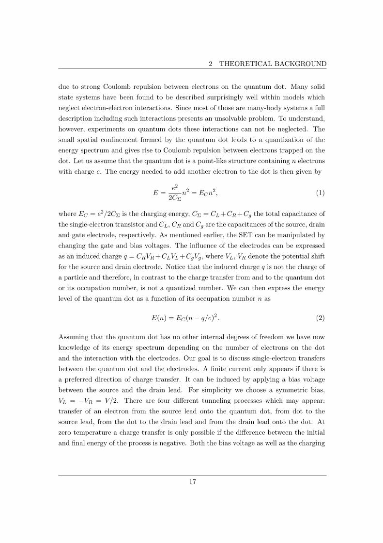
n = 0 n = 1 n = 2
0 1 2
q/e
−2
0
2eV
/EC
Figure 3: Coulomb diamonds for the single-electron transistor formed by the borderbetween conducting (white) and blocked (blue) regions.
indicate a Coulomb blockade where the conductance of the device vanishes. Analyzing
the Coulomb diamonds can yield information about the charge state and the charging
energy of the device. Due to the symmetric structure, it is therefore possible to identify
the energy as a function of the number of electrons, see Eq. (2), by analyzing only the
first two charge states. Additionally, we see that the regime of sequential tunneling of
electrons (as in Figure 2 (b) and (c)) also yields the form of a diamond.
So far, we have argued that the current in the Coulomb blockade regime vanishes.
Our argument was based on weak system-lead interactions and zero temperature. Fi-
nite temperatures, however, induce thermal fluctuations in the energy of the electrons.
Previously, we have identified the possibilities for charge transfer by using energy conser-
vation. The energy fluctuations due to finite temperatures now soften these conditions.
For this reason, experimental measurements of the Coulomb diamonds can find small
but finite currents in the Coulomb blockade regime. There is, however, a second effect
which can lead to finite currents in the blocked region. The origin of this effect are
cotunneling processes. Even though we have used classical arguments for the charging
energy, the SET is a quantum mechanical system. While a single electron is bound to
the law of energy conservation, it is possible for two or more electrons to tunnel simul-
19

2.2 Vibrational Sidebands and Spin-Polarized Currents
taneously. The tunneling electrons then do not need to conserve energy individually
but only as a whole, thereby giving rise to new contributions to the charge current.
These are called cotunneling contributions and are of higher order in the system-lead
interaction than the sequential tunneling contributions we have discussed so far. In
this thesis, we will concentrate on sequential tunneling only. It is however important
to be aware of the existance of cotunneling effects. They become important for strong
system-lead interactions or when all other transitions are forbidden. In order to stay
in the sequential tunneling regime, it is therefore necessary to enforce that the system-
lead interaction is weak compared to all other energyscales in the problem, including
the temperature of the system. In the free transport regime, sequential tunneling con-
tributions then dominate the system dynamics since the cotunneling contributions are
of quadratic or higher order in the system-lead interaction and therefore smaller than
the first order contributions. In the Coulomb blockade regime, where the sequential
tunneling contributions can vanish, however, cotunneling can become important. Here,
finite sequential tunneling contributions can be generated via thermal flucuations. If
the thermal energy is larger than the system-lead coupling strength, these contributions
dominate the cotunneling effects which can then safely be ignored.
2.2. Vibrational Sidebands and Spin-Polarized Currents
We have illustrated the basic mechanism of single-electron transport and some of its
qualitative effects using the example of the single-electron transistor. The model which
we used for the single-electron transistor does not include spin-polarized transport or
interactions between vibrational and electronic degrees of freedom. The main topic of
this thesis, however, is to investigate nanotransport in systems including both magnetic
and vibronic degrees of freedom simultaneously. A review of the literature analyzing the
effects of each of these two components on quantum transport will help to understand
the results presented throughout this thesis. In the following we therefore review selected
literature on each of these topics.
2.2.1. Franck-Condon Blockade
Previously we have argued how single-electron transfer allows us to make a connection
between the energy spectrum of a quantum dot and its current-voltage characteristics.
The current flow through a nanoelectric device such as the SET can be blocked as a
result of Coulomb interactions. By varying the bias and gate voltages, the Coulomb
20
2 THEORETICAL BACKGROUND
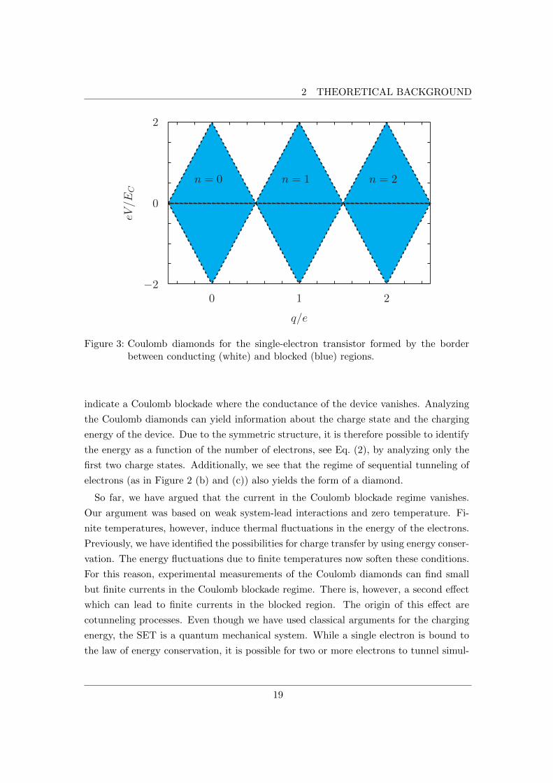
Figure 4: Schematic of a quantum dot (QD) embedded on a nanobeam with frequencyω. Bias (V ) and gate (Vg) voltage couple electronic charge flow through thequantum dot to the vibrations of the nanobeam. The resulting shift of theoscillator equilibrium position can induce a phonon blockade of the current.
blockade can be lifted. The emerging structure is known as Coulomb diamonds and
yields information about the energetic position of the charge states of the SET. A
blockade of the charge current however can also be induced by interactions between
electronic and mechanical degrees of freedom. An example for a system where such an
effect occurs is a nanomechanical resonator coupled to a single-electron transistor as
schematically shown in Figure 4. The electrostatic potential induced by the gate elec-
trode of the SET induces a force Fe on the charges. If the single-electron transistor is
embedded on the nanoresonator, the induced force will lead to a shift of the equilibrium
position of the resonator. In the same way, any vibration of the nanoresonator will
lead to a shift of the energies of the SET. If this shift is sufficiently strong, transport
through the SET is prohibited and a phonon blockade occurs. For quantum oscillators
in the regime of a strong coupling between electronic and vibrational degrees of freedom
such effects have been predicted [7, 8] and measured in molecular devices [16, 23, 24].
A strong electron-phonon coupling leads to a suppression of the current known as the
Franck-Condon blockade [9, 13, 15]. Furthermore, the eigenfrequency of the oscillator
can be read from the current-voltage characteristics of such devices. Each charge state
of the SET is coupled to the vibrational states of the nanoresonator. These vibrational
21
2.2 Vibrational Sidebands and Spin-Polarized Currents
sidebands create additional transport channels. A signature of this effect can be found
as equidistant steps in the current, separated by the eigenfrequency of the vibrational
mode, referred to as Franck-Condon steps. The same model can be used to describe
transport through molecules where the occupation of different orbitals affects the vi-
brational modes of the molecule and vice versa. The phonon blockade vanishes for very
weak electron-phonon interactions or in the limit of high temperatures. In the regime of
strong coupling between leads and nanodevice or in the strong electron-phonon coupling
regime, Franck-Condon effects become more pronounced and the phonon blockade dom-
inates the transport properties of the nanodevice or molecule. Further enhancement of a
phonon-induced current blockade is possible by driving the nanoresonator into the Euler
buckling instability [19, 21]. Here, the frequency of the fundamental bending mode of
the oscillator softens and a strong enhancement of the current noise can be found [20].
2.2.2. Spin-Polarized Currents
So far we have considered electrons as spinless fermionic particles. In the following
two chapters, we aim to discuss spin-polarized transport through nanodevices. A spin-
polarized current can be generated by using ferromagnetic leads. A ferromagnetic solid
is characterized by a different density of states for different spin carriers. One typically
distinguishes between electrons carrying a spin pointing upwards on the quantization
axis and electrons with a spin pointing downwards on the quantization axis. In a non-
magnetic solid, the density of states at the Fermi level for both types is equal. In a
ferromagnetic solid, the density of states for one spin direction is higher than for the
other. The spin directions can then be referred to as majority and minority spins. The
relative difference in the density of states between majority and minority spin carriers
is called the polarization.
Let us next replace the lead electrodes of the SET by ferromagnetic leads with a high
degree of polarization. Let us further assume that the source and the drain lead are fully
polarized in opposite directions. If now an electron tunnels from the source lead onto the
dot, its spin will point in the direction of the majority spin of the source electrode. The
drain electrode is polarized into the opposite direction. For a fully polarized material
this means that the density of states for minority spin carriers is equal to zero. The
electron on the dot therefore has no possibility to tunnel into the drain since there
are no states available. The polarization of the leads thus creates a spin-blockade. Spin
blockades and related phenomena have been observed in both single and double quantum
dot setups [61, 62]. Combining ferromagnetic leads with an external magnetic field or
22
2 THEORETICAL BACKGROUND
a local magnetization on the quantum dot can lead to precession of the electronic spin
[27, 28]. These effects are induced by noncollinear orientations of the lead polarizations
and/or an external magnetic field. It can be shown that the linear conductance of a spin
valve depends heavily on the relative angle between the leads magnetization directions.
Different orientations of the lead polarizations lead to spin accumulation on a quantum
dot or spin valve [32, 33, 63]. Signatures of a spin accumulation can be found in both
the current as well as the current noise. The interactions between the nanodevice and
the ferromagnetic leads can be expressed as an effective magnetic field acting on the
magnetic degrees of freedom of electrons or local impurity spins [30, 31] on the device.
Here, the charging energy of the device plays an important role as found in analytic
calculations of the effective field. This leads to the possibility to create nanodevices and
spin-valves with negative differential conductance [64].
2.3. Quantum Master Equation
In order to make both qualitative and quantitative statements about systems away
from thermal equilibrium such as the ones in the previously reviewed literature, it is
necessary to formulate a theoretical framework for analytical or numerical calculations.
The framework used throughout this thesis is provided by the quantum master equation
approach. To provide a clear and transparent view over our results, we therefore have to
explain the basic concept of the master equation. In the following, we derive a quantum
master equation for the reduced density matrix of an open quantum system.
2.3.1. Derivation
The first step of our derivation is to identify the system which we want to investigate.
A common approach to describe open quantum systems is the system-bath model [65].
Let us assume that we have a nanodevice coupled to two electronic charge reservoirs
by tunnel junctions. The Hamiltonian for the system and the environment can then be
written as
H = Hsys +Hlead +Hint, (3)
where Hsys represents the nanodevice, Hlead the electronic leads and Hint the interaction
between the system and the leads. The Hamiltonian of the system Hsys = Hsys(A,A†)
is a function of the electron annihilation and creation operators A, A†, respectively. At
this point, it is not necessary to give a more specific definition of the system. As we
23
2.3 Quantum Master Equation
have already seen in our analysis of the SET, the energy spectrum of the nanodevice is
of importance. We define the eigenenergies εχ of the system by Hsys|χ〉 = εχ|χ〉, where
|χ〉 are the eigenstates of the nanodevice. The leads are modelled as non-interacting
Fermi gases in the form of
Hlead =∑k,α
εk,αB†k,αBk,α, (4)
where Bk,α and B†k,α are the annihilation and creation operators for electrons in lead
α with wavevector k, and εk,α defines the chemical potential. The Hilbert space of
the system and the environment is then spanned by the product of the corresponding
eigenstates |ψ〉 = |ϕ〉|χ〉. Interactions between the system and the environment consist
of the exchange of electrons. This is described by the interaction Hamiltonian
Hint =∑k,α
(tk,αA
†Bk,α + h.c.), (5)
where tk,α is the tunneling amplitude. In contrast to the previous section we have
now chosen an explicit form for the interaction between system and environment. The
interaction Hamiltonian (5) describes the tunneling of an electron between system and
lead. A full description of the system and the environment is, in most cases, impossible
due to the size of the environment. It is, however, possible to describe the dynamics
of only the system by integrating out the environment. An approach based on this
technique is the quantum master equation [66]. The master equation describes the
evolution of the reduced density matrix via transition rates between the system and the
environment. The reduced density matrix is obtained by tracing over the degrees of
freedom of the environment, ρ(t) = Trl [W(t)], where Trl [...] denotes the trace over the
leads. The master equation can be derived starting with the Liouville-von-Neumann
equation for the full density operator W (t) in the interaction picture
W I(t) = − i~[HIint(t),W
I(t)], (6)
where the superscript I denotes operators in the interaction picture defined as OI(t) =
eiH0(t−t0)/~O(t)e−iH0(t−t0)/~ with H0 = H −Hint. The formal solution of this equation
24
2 THEORETICAL BACKGROUND
can be found by integration
W I(t) = W I0 −
i
~
∫ t
t0
dt′[HIint(t
′),W I(t′)]. (7)
Now, it is possible to reinsert the solution into Eq.(6) and iterate the equation. One
obtains
W I(t) = − i~[HIint(t),W
I0
]− 1
~2
∫ t
t0
dt′[HIint(t),
[HIint(t
′),W I(t′)]]. (8)
Notice that this equation is formally exact since all orders of the system-lead interaction
are included either explicitly in form of the interaction Hamiltonian or implicitly in the
density matrix. Since the goal is the derivation of an equation of motion for the reduced
density matrix, the next step is to trace over the lead degrees of freedom. A general
assumption at this point is to consider each lead itself to be at thermal equilibrium at all
times. In order for this assumption to be valid two conditions need to be fulfilled: First,
the equilibration time of the leads needs to be fast compared to the time between two
tunneling processes. Second, the leads need to be very large compared to the system.
The addition or removal of a finite number of electrons from the leads must not change
their state. Alternatively, we can place the leads in thermal contact with an infinitely
large superbath, which enforces a thermal distribution. Since we are discussing the
transfer of single electrons between a nanosystem and its environment typically given
by solids of macroscopic dimension, these assumption are valid. The density operator
of the leads is then given by the equilibrium distribution ρeqlead = 1Zle−βHlead with the
partition function Zl = Trl
[e−βHlead
]and β = (kBT )−1. In order to proceed, we now
assume that the initial density operator W0 = W (t = 0) can be factorized into the
density operator of the subsystem ρ(t) = Trl[W (t)] and the equilibrium distribution of
the leads, W0 = ρeqlead ⊗ ρ(t = 0). The interaction Hamiltonian Hint is non-diagonal
in the eigenbasis of the leads. Consequently, the first term on the right-hand side of
Eq. (8) vanishes if we trace over the lead degrees of freedom, leading to
ρ(t) = − i~
[H0, ρ(t)]− 1
~2Trl
∫ t
t0
dt′[HIint(t),
[HIint(t
′),W I(t′)]]
. (9)
The first term on the right-hand side appears when transforming the reduced density
matrix on the left-hand side back into the Schrodinger picture. Equation (9) is the quan-
tum master equation for the reduced density matrix. The first term describes reversible
25
2.3 Quantum Master Equation
motion and yields coherent oscillations between quantum states of the subsystem. It
contains no information about the bath or dissipative effects. The second term contains
all interactions between the bath and the system. It gives rise to irreversible dynamics
and effects like relaxation, decoherence or dephasing. Approximate solutions to the
master equation can be found in various ways. A review of different types of master
equations and the corresponding solution methods is given in Ref.[67].
2.3.2. Redfield Master Equation
The approach pursued in this thesis is the numerical solution of the Redfield master
equation by using diagrammatic perturbation theory. The Redfield equation follows
from the master equation (9) by making two approximations.
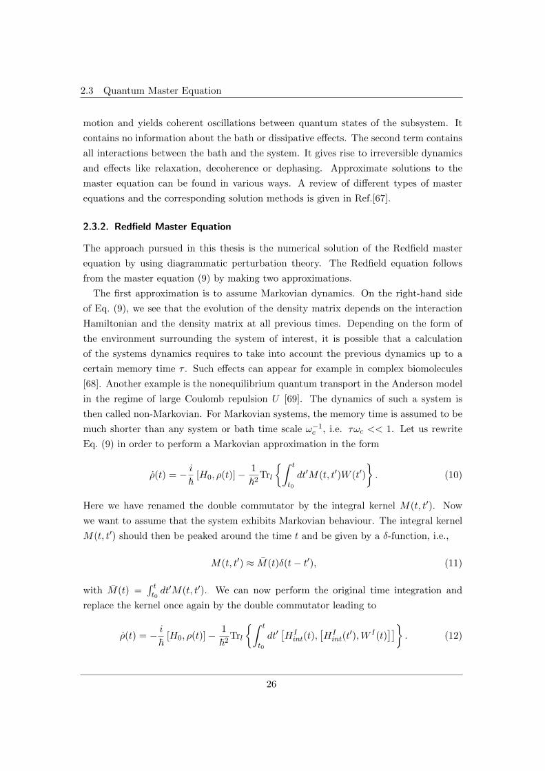
The first approximation is to assume Markovian dynamics. On the right-hand side
of Eq. (9), we see that the evolution of the density matrix depends on the interaction
Hamiltonian and the density matrix at all previous times. Depending on the form of
the environment surrounding the system of interest, it is possible that a calculation
of the systems dynamics requires to take into account the previous dynamics up to a
certain memory time τ . Such effects can appear for example in complex biomolecules
[68]. Another example is the nonequilibrium quantum transport in the Anderson model
in the regime of large Coulomb repulsion U [69]. The dynamics of such a system is
then called non-Markovian. For Markovian systems, the memory time is assumed to be
much shorter than any system or bath time scale ω−1c , i.e. τωc << 1. Let us rewrite
Eq. (9) in order to perform a Markovian approximation in the form
ρ(t) = − i~
[H0, ρ(t)]− 1
~2Trl
∫ t
t0
dt′M(t, t′)W (t′)
. (10)
Here we have renamed the double commutator by the integral kernel M(t, t′). Now
we want to assume that the system exhibits Markovian behaviour. The integral kernel
M(t, t′) should then be peaked around the time t and be given by a δ-function, i.e.,
M(t, t′) ≈ M(t)δ(t− t′), (11)
with M(t) =∫ tt0dt′M(t, t′). We can now perform the original time integration and
replace the kernel once again by the double commutator leading to
ρ(t) = − i~
[H0, ρ(t)]− 1
~2Trl
∫ t
t0
dt′[HIint(t),
[HIint(t
′),W I(t)]]
. (12)
26
2 THEORETICAL BACKGROUND
The second approximation we want to perform is a weak-coupling approximation. If the
contact between the system and the environment is sufficiently weak, it is reasonable
to assume that only the lowest order of the interaction is important for the system’s
dynamics. We will therefore assume that the density matrix W I(t) does not depend
on the system-lead interaction. Consequently, since we have iterated the equation only
once, this assumption yields the master equation to lowest order in the system-lead
interaction and is only valid when the interaction strength tk,α is weak compared to
other energy scales in the problem. The evolution of the reduced density matrix can now
be determined by expanding the double commutator and performing the integration.
Carrying out the trace over the bath degrees of freedom and using the factorization of
the density matrix finally yields the Redfield equation for the components of the reduced
density matrix in the form
ρab(t) = − i~
(εa − εb)ρab(t)−∑cd
Rabcdρcd(t). (13)
Here Rabcd, denotes the Redfield tensor containing the rates obtained by evaluating the
second term on the right hand side of Eq.(12). The indices a, b, c, d refer to energy
eigenstates of the system Hamiltonian. The Redfield equation has many applications in
physics and chemistry. It is a well-established method to describe processes like nuclear
magnetic resonance [70], optical methods [71] or quantum transport in nanodevices
[67]. In nuclear magnetic resonance, the Redfield equation can be used to describe the
relaxation dynamics of the spin system in a paramagnetic environment. In a similar
way the dynamics of optically excited systems can be determined by a set of equation
derived from the Redfield approach. These equation are known as the optical Bloch
equations [72]. Transfer of excitation energy in biomolecules can also be investigated
by using of the Redfield equation [73].
2.3.3. Diagrammatic Perturbation Theory
One particular way of obtaining the Redfield rates is the diagrammatic perturbation
theory [58]. The rates which form the Redfield tensor can be represented by Feynman
diagrams [66, 74] up to first order in the tunneling. In order to understand this method
we first have to give a brief introduction into diagrammatic methods for equilibrium
dynamics and then introduce the corresponding method for non-equilibrium physics
[75].
27
2.3 Quantum Master Equation
Feynman diagrams have been developed by R. Feynman in 1948 as a tool to sim-
plify the calculation of Green’s functions in quantum field theory. A Green’s function
G(x, t;x′, t′) describes the time evolution of a system from time t′ at x′ to a state x
at time t. Let us assume a scattering problem: We have a system or particle which
interacts with a different particle at time t = 0 given by the interaction V (t). Initially,
at t→ −∞, both particles are separated and do not interact. The same is valid for very
long times after the scattering process, t → ∞. We can then define the time-ordered
Green’s function as
G(x, t;x′, t′) = − i~
〈Ψ0|TψH(x, t)ψ†H(x′, t′)
|Ψ0〉
〈Ψ0|Ψ0〉, (14)
where T denotes the time-ordering operator, |Ψ0〉 the ground state of the system and
ψH(x, t) the field operator in the Heisenberg picture. The definition of the Green’s
function contains the exact ground state of the system which is one of the quantities
that one usually wants to calculate using the Green’s function. However, we can express
the ground state of the interacting system in terms of the ground state of the non-
interacting system |Φ0〉 and the scattering matrix S(t, t′). According to the Gell-Mann
and Low theorem, the ground state is given by
|Ψ0〉 = S(0,−∞)|Φ0〉. (15)
We then find for the time-ordered Green’s function
G(x, t;x′, t′) = − i~〈Φ0|T
S(∞,−∞)ψ(x, t)ψ†(x′, t′)
|Φ0〉
〈Φ0|S(∞,−∞)|Φ0〉. (16)
This new expression allows us to calculate the Green’s function by performing a pertur-
bative expansion in the interaction V (t). We expand the scattering matrix according
to
S(∞,−∞) =∞∑n=0
(−i)n+1
n!
∫ ∞−∞
dt1...dtnT V (t1)...V (tn) . (17)
Each interaction term contains several field operators ψ(t). In order to calculate the
time evolution of the system, we therefore need to be able to determine expectation
28

2 THEORETICAL BACKGROUND
Figure 5: Graphical representation of the free Green’s function (a), the full Green’sfunction (b) interaction (c).
values of the type
〈Φ0|Tψ(t)ψ†(t′)ψ†(t1)ψ†(t2)ψ(t2)ψ(t1)
|Φ0〉, (18)
and similar expressions. The Wick theorem [76] states that these expressions are given
by the sum of all pairwise contractions. Finding all contractions can become a tedious
and complicated task depending on the complexity of the system. The Feynman dia-
grams, however, are pictorial representations of exactly these expectation values. Each
diagram denotes a very specific contribution of our expansion. Figure 5 shows the most
fundamental components for diagrams needed to describe the scattering problem. Us-
ing only these tools it is possible to write down a graphical representation of the Dyson
equation [77] as shown in Figure 6.
The discussion up to this point refers to the use of the diagrammatic representation in
equilibrium systems. Our brief motivation, however, already illustrates the fundamental
difference and difficulty we have to face when we want to apply the method to non-
equilibrium physics. In our derivation of a pertubation series for the Green’s function,
the scattering matrix plays a central role. In equilibrium, we were able to rewrite the
exact ground state of the system due to the fact that it relaxes into its initial ground
state for infinitely large times. In non-equilibrium, however, this is not possible. There
is no guarantee that the system returns to its initial state at any time. A solution of
this problem can be found in form of the Keldysh technique. Instead of defining the
time-ordered Green’s function, we define a contour ordered Green’s function. Instead
of going from an initial time t0 to a final time tf as shown in Figure 7 (a), the Keldysh
contour goes back to the initial time t0 as shown in Figure 7 (b). Setting the initial
time to minus infinity (t0 → −∞) now allows us to use the perturbation series of the
29
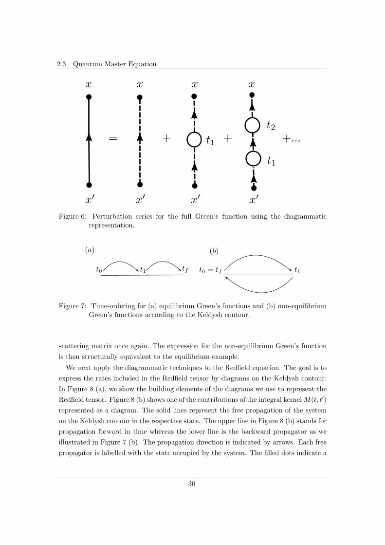
2.3 Quantum Master Equation
Figure 6: Perturbation series for the full Green’s function using the diagrammaticrepresentation.
Figure 7: Time-ordering for (a) equilibrium Green’s functions and (b) non-equilibriumGreen’s functions according to the Keldysh contour.
scattering matrix once again. The expression for the non-equilibrium Green’s function
is then structurally equivalent to the equilibrium example.
We next apply the diagrammatic techniques to the Redfield equation. The goal is to
express the rates included in the Redfield tensor by diagrams on the Keldysh contour.
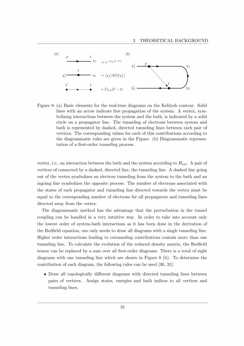
In Figure 8 (a), we show the building elements of the diagrams we use to represent the
Redfield tensor. Figure 8 (b) shows one of the contributions of the integral kernelM(t, t′)
represented as a diagram. The solid lines represent the free propagation of the system
on the Keldysh contour in the respective state. The upper line in Figure 8 (b) stands for
propagation forward in time whereas the lower line is the backward propagator as we
illustrated in Figure 7 (b). The propagation direction is indicated by arrows. Each free
propagator is labelled with the state occupied by the system. The filled dots indicate a
30
2 THEORETICAL BACKGROUND
Figure 8: (a) Basic elements for the real-time diagrams on the Keldysh contour. Solidlines with an arrow indicate free propagation of the system. A vertex, sym-bolizing interactions between the system and the bath, is indicated by a solidcircle on a propagator line. The tunneling of electrons between system andbath is represented by dashed, directed tunneling lines between each pair ofvertices. The corresponding values for each of this contributions according tothe diagrammatic rules are given in the Figure. (b) Diagrammatic represen-tation of a first-order tunneling process.
vertex, i.e., an interaction between the bath and the system according to Hint. A pair of
vertices of connected by a dashed, directed line, the tunneling line. A dashed line going
out of the vertex symbolizes an electron tunneling from the system to the bath and an
ingoing line symbolizes the opposite process. The number of electrons associated with
the states of each propagator and tunneling line directed towards the vertex must be
equal to the corresponding number of electrons for all propagators and tunneling lines
directed away from the vertex.
The diagrammatic method has the advantage that the perturbation in the tunnel
coupling can be handled in a very intuitive way. In order to take into account only
the lowest order of system-bath interactions as it has been done in the derivation of
the Redfield equation, one only needs to draw all diagrams with a single tunneling line.
Higher order interactions leading to cotunneling contributions contain more than one
tunneling line. To calculate the evolution of the reduced density matrix, the Redfield
tensor can be replaced by a sum over all first-order diagrams. There is a total of eight
diagrams with one tunneling line which are shown in Figure 8 (b). To determine the
contribution of each diagram, the following rules can be used [30, 31]:
• Draw all topologically different diagrams with directed tunneling lines between
pairs of vertices. Assign states, energies and bath indices to all vertices and
tunneling lines.
31
2.3 Quantum Master Equation
• Each propagator on the Keldysh contour with state χ from time t′ to t implies a
factor e−iεχ(t−t′).
• Each vertex between two states χ and χ′ containing a system operator A implies a
factor 〈χ′|A|χ〉, where χ is the incoming and χ′ the outgoing state on the Keldysh
contour.
• A directed tunneling for reservoir α from t′ to t implies a factor Ck,α(t′−t) for tun-
neling lines forward and C†k,α(t− t′) for tunneling lines backward on the Keldysh
contour. Here, Ck,α(t− t′) = 〈B†k,α(t)Bk,α(t′)〉 denotes the bath correlation func-
tion at wavevector k.
• Each diagram carries a prefactor −(−1)m where m is the number of vertices on the
lower contour. Additional minus signs can appear due to ordering of the electronic
operators in the case of multi-electron states.
• Sum over all combinations of ingoing and outgoing states. Each diagram has to
be integrated over the time∫ tt0dt′.
Let us compare the diagrammatic rules with the results obtained by expanding the
double commutator in Eq. (12) in order to understand their origin. The double com-
mutator reads
[HIint(t),
[HIint(t
′),W I(t)]]
= HIint(t)H
Iint(t
′)W I(t)−HIint(t)W
I(t)HIint(t
′)
−HIint(t
′)W I(t)HIint(t) +W I(t)HI
int(t′)HI
int(t). (19)
By inserting the definition of the interaction Hamiltonian (5), the third term yields
〈ϕ|HIint(t
′)W I(t)HIint(t)|ϕ〉 =
|tk,α|2∑
k〈ϕ|A†(t′)Bk,α(t′)W (t)B†k,α(t)A(t) +B†k,α(t′)A(t′)W (t)A†(t)Bk,α(t)|ϕ〉,(20)
where we have now omitted the superscript for the interaction picture. Due to the trace
over the bath all pairings of two lead electron annihilation or two lead electron creation
operators vanish. Using the factorization of the density matrix leads to
〈ϕ|Hint(t′)W (t)Hint(t)|ϕ〉 =
|tk,α|2∑
k
[A†(t′)A(t)ρ(t)C†k,α(t′ − t) +A(t′)A†(t)ρ(t)Ck,α(t′ − t)
]. (21)
32
2 THEORETICAL BACKGROUND
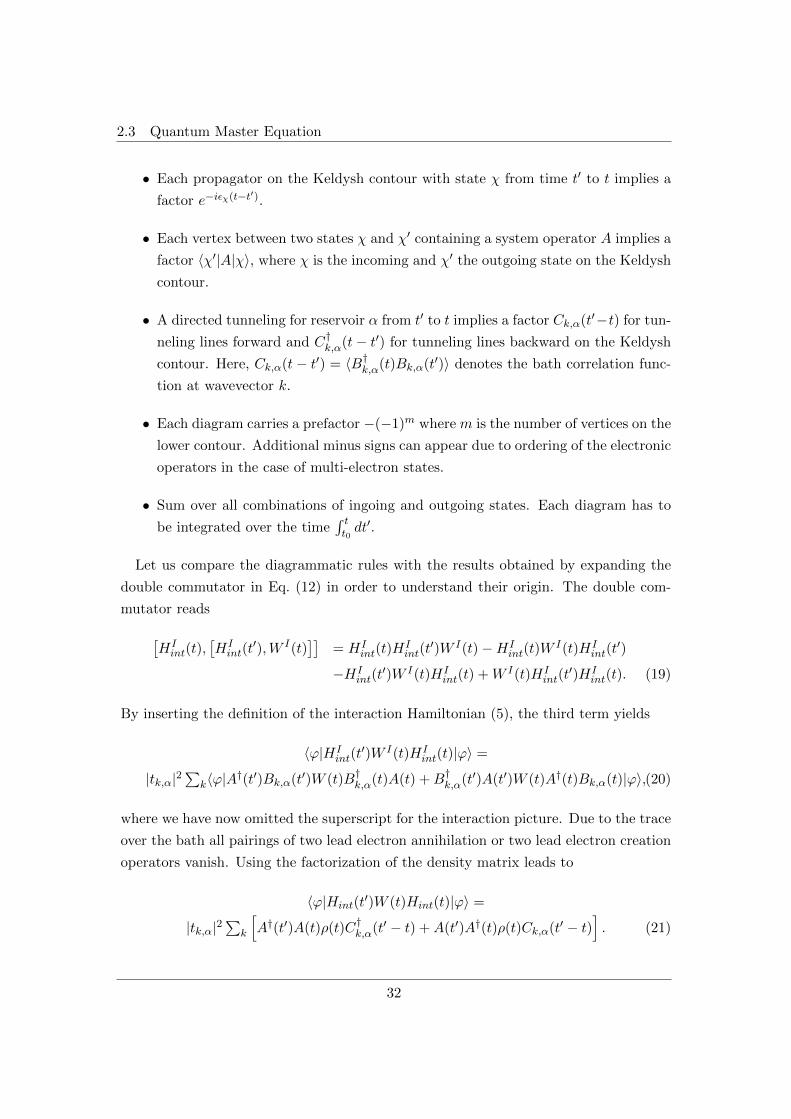
Figure 9: Schematic of all eight different diagrams contribution to the first order tran-sitions in the master equation.
The second term on the right-hand side describes the diagram depicted in Figure 8 (b).
All other diagrams can be found in the same way via the expansion of the commuta-
tor. Drawing all topological diagrams and applying the diagrammatic rules is therefore
equivalent to a direct calculation of the Redfield tensor. A schematic of all different
first-order diagrams appearing in the master equation of our system is shown in Figure
9. Since the Feynman diagrams are an exact representation of the perturbation theory
in the system-lead interaction, it would in principle be possible to calculate the next
order in the tunnel coupling by drawing all diagrams with two tunneling lines. Due to
the large amount of combinations, a diagrammatic approach yields a huge advantage
over a direct calculation of the resulting commutators. In this thesis, however, we will
restrict ourselves to the first order contributions.
2.3.4. Numerical Solution
The Redfield equation (13) gives rise to a set of coupled differential equations for the
elements of the reduced density matrix of our nanodevice. For small systems an an-
alytical solution is possible [28, 30, 57]. Depending on the dimension of the Hilbert
space of the system, however, a numerical calculation is preferable. In the following we
therefore discuss briefly how to find a numerical solution for the full Redfield equation.
The stationary solution of the master equation is given by
0 = Rρstat(t), (22)
where we have absorbed the zeroth order term describing the coherent dynamics of the
quantum system into the modified Redfield tensor R. To simplify numerical calcula-
tions we rearrange the density operator into a vector ρstat(t) such that the Redfield
33
2.3 Quantum Master Equation
tensor becomes a matrix. The calculation of the stationary solution then reduces to
an eigenvalue problem for the matrix R. Finding the eigenvalues of a matrix is a task
which can be fulfilled by common numerical methods.
To determine the time evolution of the reduced density operator, we first find the
formal solution of the Redfield equation
ρ(t) = eR(t−t0)ρ(t = 0). (23)
The formal solution can be expanded in terms of the left and right eigenvectors of R,
such that
ρ(t) =∑m
v†mLρ(t0)eΓm(t−t0)vRm, (24)
where vL/Rm denote the the left/right eigenvectors and Γm the eigenvalues of the mod-
ified Redfield tensor. Knowledge of the time evolution of the reduced density matrix
then allows us to calculate expectation values of any operators, such as, for example,
average spin projections, the number of electrons on a quantum dot or the occupation
of vibrational states. Using diagrammatic methods, it is also possible to determine the
charge current flowing through the device. The charge current can be defined as the
time derivative of the number of electrons on the nanodevice,
I = e〈∂n∂t〉. (25)
The change in the electronic occupation number n can be determined by summing over
all diagrams in which the number of electrons on the device changes between t′ and t,
i.e. the four diagrams on the left side of Figure 9. The average charge current is then
given by the expectation value of these contributions.
By this, we have now a method at hand which allows us to calculate the expectation
value of any system operator both in the steady state as well at any other given time.
The method requires knowledge of the bath correlator, the system-bath interaction
and the eigenenergies of the system only. We are, however, limited to a description of
systems which interact weakly with their environment and are dominated by Markovian
dynamics.
34
3 COOLING NANODEVICES VIA SPIN-POLARIZED CURRENTS
3. Cooling Nanodevices via spin-polarized Currents
The continuous effort of miniaturizing electronic devices leads to several new challenges.
One of these challenges is the requirement to develop efficient cooling mechanisms for
micro- and nanoelectronics. To date most electronic devices utilize passive cooling tech-
niques. Thermal contact with the supporting structure provides the possibility to use
the environment as a passive heat sink. Active or dynamical nano-cooling has received
little attention, although passive thermal transport is inefficient at the nanoscale. Fur-
thermore, most of the recently developed electronic and magnetic nanodevices operate
at low temperatures only. The importance of a dynamical cooling mechanism on the
nanoscale can therefore not be underestimated. Dynamical nanorefrigerators would also
open the possibility for new experiments and devices. Most dynamical cooling methods
require spacious equipment and mechanical movement (of pumping equipment, for ex-
ample) thus making them impractical for an application on nanodevices. Manipulating
the heat on the nanoscale would then not only drastically decrease the size of the cooling
equipment, but also yield the possibility to create arrays of cooled nanodevices.
The most accessible part of many nanodevices are the electronic degrees of free-
dom. By applying external bias voltages, it is often not only possible to control charge
currents, but also magnetic or mechanical properties. There are proposals for nanore-
frigerators in which heat is carried by an electronic charge current [36]. In this work, we
propose a cooling mechanism which utilizes the electronic spin rather than the charge
in order to achieve a net cooling effect. The cooling mechanism is a nanoscale adaption
of the magnetocaloric demagnetization cooling [40] which is an example of a successful
cooling method on the macroscale using magnetic degrees of freedom.
The chapter is structured as follows. In the first section, we motivate the cooling
concept by explaining the magnetocaloric demagnetization cooling and discussing an
adaption to the nanoscale. A proof of principle model for the nanocooling scheme is
introduced in the second section. The model is compared with recent experiments [41–
43, 78]. We analyze the energy spectrum and give a brief synopsis of the numerical
method in the third section. The fourth and fifth section are dedicated to a description
of the principle mechanism of the cooling setup and its initial preparation, respectively.
Section 3.6 displays the numerical results. We compare different lead setups with respect
to their cooling efficiency and identify the most favourable cooling setup. As the main
result of this chapter, we show a decrease of the effective temperature to about 50%
of its initial value. A summary and conclusion of the results is provided in the final
35
3.1 Cooling Scheme
section.
3.1. Cooling Scheme
Using the spin degree of freedom to cool a macroscopic sample of matter is a mechanism
which first has been suggested in 1927 by Peter Debye and William F. Giauque [79].
The mechanism is known as demagnetization cooling and lead to the development of
the first magnetic refrigerators with the ability to cool samples to temperatures below
0.3 K. These magnetic refrigerators utilize changing magnetic fields in order to invoke
a change in temperature. The core principle of the demagnetization cooling is the
transformation of thermal energy into magnetic energy in an isolated sample as part
of a reorientation process of the magnetic moments. In order to develop a magnetic
refrigerator a thermodynamic cycle can be built around this principle. An example of
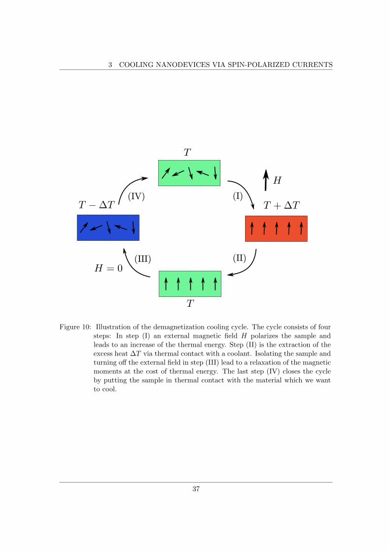
such a cooling cycle (see Figure 10) consists of four steps:
(I) Adiabatic magnetization: A magnetic substance is placed in an isolated environ-
ment without any thermal contact. An increasing external magnetic field H causes
the magnetic moments of the substance to align. Since the substance is isolated, both
the entropy and the energy have to be conserved. This leads to an increase in the
temperature (T → T + ∆T ) to compensate for the decrease in the magnetic entropy.
(II) Isomagnetic enthalpic transfer: In order to remove the added heat it is necessary
to bring the substance in thermal contact with a coolant. The magnetic field is held
constant during this phase in order to keep the magnetic moments from reabsorbing the
heat. Once the magnetic solid is cooled down to its initial temperature (T + ∆T → T )
the coolant can be removed thus once again isolating the magnetic substance.
(III) Adiabatic demagnetization: In the third step, the magnetic field is decreased
causing the magnetic moments to overcome the field. Since both energy and entropy
are once again conserved the relaxation of the magnetic moments leads to a decrease of
the temperature (T → T −∆T ) in the substance.
(IV) Isomagnetic entropic transfer: Now, the magnetic field is held constant and the
substance is brought into thermal contact with the sample which is to be cooled. The
resulting heat exchange cools the sample, while bringing the solid back to its original
temperature (T − ∆T → T ). Once a thermal equilibrium is reached the cycle can be
restarted.
While being successfully applied on the macroscale, a conceptual difficulty of these
magnetic refrigeration cycles is the opening and closing of heat links. In a macroscopic
setup, the transfer of the excess heat to a coolant (step (II)) requires either to pump
36
3 COOLING NANODEVICES VIA SPIN-POLARIZED CURRENTS
(I)
(II)(III)
(IV)
Figure 10: Illustration of the demagnetization cooling cycle. The cycle consists of foursteps: In step (I) an external magnetic field H polarizes the sample andleads to an increase of the thermal energy. Step (II) is the extraction of theexcess heat ∆T via thermal contact with a coolant. Isolating the sample andturning off the external field in step (III) lead to a relaxation of the magneticmoments at the cost of thermal energy. The last step (IV) closes the cycleby putting the sample in thermal contact with the material which we wantto cool.
37
3.1 Cooling Scheme
the coolant or mechanical movement of the magnetic substance. In the same way,
thermal contact between substance and sample (step (IV)) has to be established. These
technical constraints of the cooling cycle complicate an adaption to the nanoscale. Here,
mechanical movement of the setup or large cooling equipment proves impractical for
most applications to nanodevices. An example would be the development of microchips
to the nanoscale where they are to be used in large numbers as part of electronic
hardware [80]. Movement of individual microchips or even arrays of microchips as
part of their cooling concept will interfere with their application. Additionally, the use
of changing external fields for magnetization hinders an application of such a cooling
scheme for magnetic memory devices.
Nonetheless, the nanocooling scheme we propose here is also based on the exchange
of energy between magnetic and phononic degrees of freedom. The core of our concept
is the use of spin-polarized currents in order to generate a magnetization. Contrary
to the macroscale cooling cycle which relies on equilibrium thermodynamics, we use
transport properties of nanodevices to develop a non-equilibrium cooling scheme. The
main advantage of a magnetization via spin-polarized currents is the ability to control
the contact between sample and environment all-electronically by using bias voltages.
This environment is represented by ferromagnetic leads or spin-polarized electron reser-
voirs. Applying a bias voltage to the leads generates the flow of a spin-polarized current
through the nanodevice. The polarized spins can interact with the local magnetization
of the device via exchange coupling thus replacing the function of the external field H
of the macroscopic setup. It is therefore possible to generate and control the magneti-
zation of the sample directly by using its charge transport properties. Additionally, the
contact to the environment allows the transfer of entropy and energy between system
and environment, thereby reducing the heat generated by the magnetization process
(step (I)). The polarization of the local magnetization of the nanodevice by the current
forces the device into the spin ground state, thereby lowering its energy. A magnetome-
chanical coupling between the local magnetization and the vibronic degrees of freedom
then enables the spins to relax again by reducing the vibrational energy and thus cooling
the device. An externally applied electric current, however, gives rise to Ohmic heating
effects. The spin-polarized current thus induces two effects: A reduction of the magnetic
energy of the device, and, a heating due to Ohmic losses. An effective cooling protocol
can only be established if the cooling effect due to magnetization exceeds the heating
generated by Ohmic losses. This is possible as will be shown in the following sections.
38
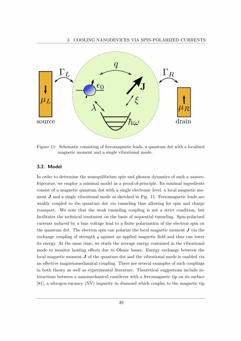
3 COOLING NANODEVICES VIA SPIN-POLARIZED CURRENTS
Figure 11: Schematic consisting of ferromagnetic leads, a quantum dot with a localizedmagnetic moment and a single vibrational mode.
3.2. Model
In order to determine the nonequilibrium spin and phonon dynamics of such a nanore-
frigerator, we employ a minimal model as a proof-of-principle. Its minimal ingredients
consist of a magnetic quantum dot with a single electronic level, a local magnetic mo-
ment J and a single vibrational mode as sketched in Fig. 11. Ferromagnetic leads are
weakly coupled to the quantum dot via tunneling thus allowing for spin and charge
transport. We note that the weak tunneling coupling is not a strict condition, but
facilitates the technical treatment on the basis of sequential tunneling. Spin-polarized
currents induced by a bias voltage lead to a finite polarization of the electron spin on
the quantum dot. The electron spin can polarize the local magnetic moment J via the
exchange coupling of strength q against an applied magnetic field and thus can lower
its energy. At the same time, we study the average energy contained in the vibrational
mode to monitor heating effects due to Ohmic losses. Energy exchange between the
local magnetic moment J of the quantum dot and the vibrational mode is enabled via
an effective magnetomechanical coupling. There are several examples of such couplings
in both theory as well as experimental literature. Theoretical suggestions include in-
teractions between a nanomechanical cantilever with a ferromagnetic tip on its surface
[81], a nitrogen-vacancy (NV) impurity in diamond which couples to the magnetic tip
39
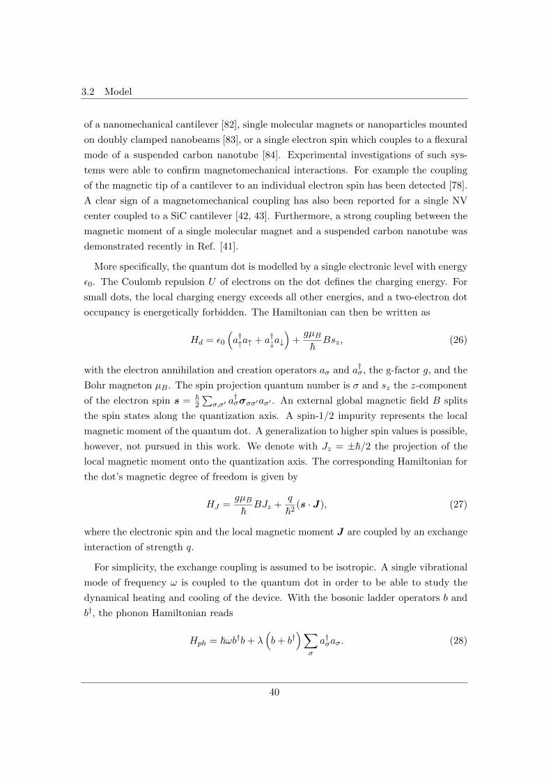
3.2 Model
of a nanomechanical cantilever [82], single molecular magnets or nanoparticles mounted
on doubly clamped nanobeams [83], or a single electron spin which couples to a flexural
mode of a suspended carbon nanotube [84]. Experimental investigations of such sys-
tems were able to confirm magnetomechanical interactions. For example the coupling
of the magnetic tip of a cantilever to an individual electron spin has been detected [78].
A clear sign of a magnetomechanical coupling has also been reported for a single NV
center coupled to a SiC cantilever [42, 43]. Furthermore, a strong coupling between the
magnetic moment of a single molecular magnet and a suspended carbon nanotube was
demonstrated recently in Ref. [41].
More specifically, the quantum dot is modelled by a single electronic level with energy
ε0. The Coulomb repulsion U of electrons on the dot defines the charging energy. For
small dots, the local charging energy exceeds all other energies, and a two-electron dot
occupancy is energetically forbidden. The Hamiltonian can then be written as
Hd = ε0
(a†↑a↑ + a†↓a↓
)+gµB~Bsz, (26)
with the electron annihilation and creation operators aσ and a†σ, the g-factor g, and the
Bohr magneton µB. The spin projection quantum number is σ and sz the z-component
of the electron spin s = ~2
∑σ,σ′ a
†σσσσ′aσ′ . An external global magnetic field B splits
the spin states along the quantization axis. A spin-1/2 impurity represents the local
magnetic moment of the quantum dot. A generalization to higher spin values is possible,
however, not pursued in this work. We denote with Jz = ±~/2 the projection of the
local magnetic moment onto the quantization axis. The corresponding Hamiltonian for
the dot’s magnetic degree of freedom is given by
HJ =gµB~BJz +
q
~2(s · J), (27)
where the electronic spin and the local magnetic moment J are coupled by an exchange
interaction of strength q.
For simplicity, the exchange coupling is assumed to be isotropic. A single vibrational
mode of frequency ω is coupled to the quantum dot in order to be able to study the
dynamical heating and cooling of the device. With the bosonic ladder operators b and
b†, the phonon Hamiltonian reads
Hph = ~ωb†b+ λ(b+ b†
)∑σ
a†σaσ. (28)
40

3 COOLING NANODEVICES VIA SPIN-POLARIZED CURRENTS
Due to the linear coupling of the electronic occupation to the oscillator position, it is
possible to excite or relax the vibrational mode with each electronic tunneling process
which populates the dot. These excitations describe the inevitable heating of the nan-
odevice due to the charge current. A relaxation of the phonon mode is possible if its
energy exceeds the thermal energy of the ferromagnetic leads. The latter is the main
mechanism used for passive heat sinks via the environment.
Energy exchange between the vibrational mode and the local magnetization is enabled
by the magnetomechanical coupling given by
HJ−ph =ξ
~
(b+ b†
)(J+ + J−) , (29)
where J± = (Jx± iJy)/2 are spin-1/2 ladder operators inducing transitions between the
magnetic states with a simultaneous relaxation or excitation of the vibrational mode.
It should be realized that equation (29) describes an effective coupling. Interactions be-
tween a vibrational mode and a spin can be the result of spin-orbit effects. Lehmann and
Loss show in Ref.[85] that a combination of electron-phonon and spin-orbit interaction
leads to an effective coupling between spin and phonons. By performing a Schrieffer-
Wolff transformation [86], it is possible to eliminate the spin-orbit coupling in lowest
order. A projection onto the orbital ground state then yields an effective spin-phonon
coupling. In this way, all contributions from higher orbital states are neglected. The
coupling constant ξ can then be derived as the ground state expectation value of a com-
bination of electron-phonon operators and the generator of the transformation. Notice
that the resulting coupling Hamiltonian as presented in Eq.(29) breaks time-reversal
symmetry which could be restored by taking into account the higher orbital states for
the electron. In this work, however, we will not focus on the origin or derivation of
the magnetomechanical coupling. In order to explore the possibilities of a nanocooling
mechanism, we use an effective description and choose both electron-phonon coupling
λ and magnetomechanical coupling ξ independently.
A comparison with existing experimental setups yields experimental values for both
coupling strengths. Ganzhorn et al. [41] have realized a set-up with a single molecular
magnet covalently bound to a carbon nanotube suspended between two leads. The
molecule has a magnetic ground state of |J | = 6 and the groundstate doublet Jz = ±6
is separated from the excited states by several hundreds of Kelvin. A relaxation or
excitation of the spin state therefore dominantly occurs via quantum spin tunneling
between those two states. The Ising-like spin flip can therefore be described effectively by
41
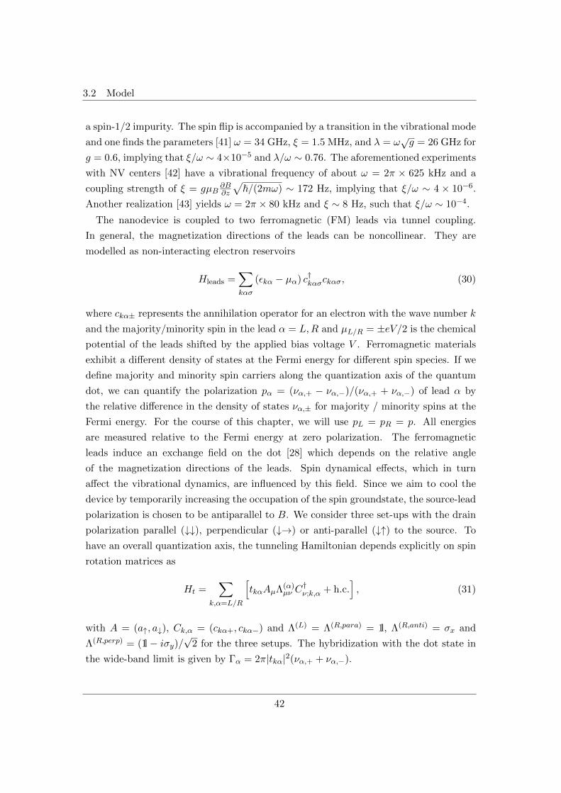
3.2 Model
a spin-1/2 impurity. The spin flip is accompanied by a transition in the vibrational mode
and one finds the parameters [41] ω = 34 GHz, ξ = 1.5 MHz, and λ = ω√g = 26 GHz for
g = 0.6, implying that ξ/ω ∼ 4×10⁻⁵ and λ/ω ∼ 0.76. The aforementioned experiments
with NV centers [42] have a vibrational frequency of about ω = 2π × 625 kHz and a
coupling strength of ξ = gµB∂B∂z
√~/(2mω) ∼ 172 Hz, implying that ξ/ω ∼ 4 × 10⁻⁶.
Another realization [43] yields ω = 2π × 80 kHz and ξ ∼ 8 Hz, such that ξ/ω ∼ 10−4.
The nanodevice is coupled to two ferromagnetic (FM) leads via tunnel coupling.
In general, the magnetization directions of the leads can be noncollinear. They are
modelled as non-interacting electron reservoirs
Hleads =∑kασ
(εkα − µα) c†kασckασ, (30)
where ckα± represents the annihilation operator for an electron with the wave number k
and the majority/minority spin in the lead α = L,R and µL/R = ±eV/2 is the chemical
potential of the leads shifted by the applied bias voltage V . Ferromagnetic materials
exhibit a different density of states at the Fermi energy for different spin species. If we
define majority and minority spin carriers along the quantization axis of the quantum
dot, we can quantify the polarization pα = (να,+ − να,−)/(να,+ + να,−) of lead α by
the relative difference in the density of states να,± for majority / minority spins at the
Fermi energy. For the course of this chapter, we will use pL = pR = p. All energies
are measured relative to the Fermi energy at zero polarization. The ferromagnetic
leads induce an exchange field on the dot [28] which depends on the relative angle
of the magnetization directions of the leads. Spin dynamical effects, which in turn
affect the vibrational dynamics, are influenced by this field. Since we aim to cool the
device by temporarily increasing the occupation of the spin groundstate, the source-lead
polarization is chosen to be antiparallel to B. We consider three set-ups with the drain
polarization parallel (↓↓), perpendicular (↓→) or anti-parallel (↓↑) to the source. To
have an overall quantization axis, the tunneling Hamiltonian depends explicitly on spin
rotation matrices as
Ht =∑
k,α=L/R
[tkαAµΛ(α)
µν C†ν;k,α + h.c.
], (31)
with A = (a↑, a↓), Ck,α = (ckα+, ckα−) and Λ(L) = Λ(R,para) = 1l, Λ(R,anti) = σx and
Λ(R,perp) = (1l − iσy)/√
2 for the three setups. The hybridization with the dot state in
the wide-band limit is given by Γα = 2π|tkα|2(να,+ + να,−).
42
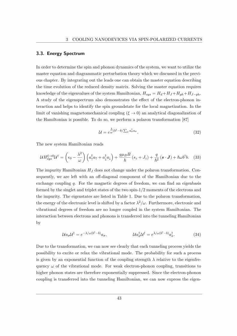
3 COOLING NANODEVICES VIA SPIN-POLARIZED CURRENTS
3.3. Energy Spectrum
In order to determine the spin and phonon dynamics of the system, we want to utilize the
master equation and diagrammatic perturbation theory which we discussed in the previ-
ous chapter. By integrating out the leads one can obtain the master equation describing
the time evolution of the reduced density matrix. Solving the master equation requires
knowledge of the eigenvalues of the system Hamiltonian, Hsys = Hd+HJ+Hph+HJ−ph.
A study of the eigenspectrum also demonstrates the effect of the electron-phonon in-
teraction and helps to identify the spin groundstate for the local magnetization. In the
limit of vanishing magnetomechanical coupling (ξ → 0) an analytical diagonalization of
the Hamiltonian is possible. To do so, we perform a polaron transformation [87]
U = eλω (b†−b)
∑σ a†σaσ . (32)
The new system Hamiltonian reads
UHξ→0sys U† =
(ε0 −
λ2
ω
)(a†↑a↑ + a†↓a↓
)+gµBB
~(sz + Jz) +
q
~2(s · J) + ~ωb†b. (33)
The impurity Hamiltonian HJ does not change under the polaron transformation. Con-
sequently, we are left with an off-diagonal component of the Hamiltonian due to the
exchange coupling q. For the magnetic degrees of freedom, we can find an eigenbasis
formed by the singlet and triplet states of the two spin-1/2 moments of the electrons and
the impurity. The eigenstates are listed in Table 1. Due to the polaron transformation,
the energy of the electronic level is shifted by a factor λ2/ω. Furthermore, electronic and
vibrational degrees of freedom are no longer coupled in the system Hamiltonian. The
interaction between electrons and phonons is transferred into the tunneling Hamiltonian
by
UaσU† = e−λ/ω(b†−b)aσ, Ua†σU† = eλ/ω(b†−b)a†σ. (34)
Due to the transformation, we can now see clearly that each tunneling process yields the
possibility to excite or relax the vibrational mode. The probability for such a process
is given by an exponential function of the coupling strength λ relative to the eigenfre-
quency ω of the vibrational mode. For weak electron-phonon coupling, transitions to
higher phonon states are therefore exponentially suppressed. Since the electron-phonon
coupling is transferred into the tunneling Hamiltonian, we can now express the eigen-
43
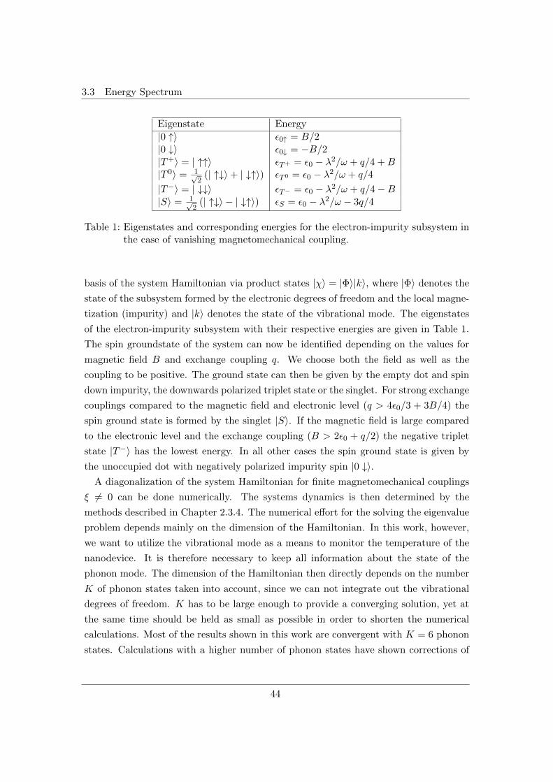
3.3 Energy Spectrum
Eigenstate Energy
|0 ↑〉 ε0↑ = B/2|0 ↓〉 ε0↓ = −B/2|T+〉 = | ↑↑〉 εT+ = ε0 − λ2/ω + q/4 +B|T 0〉 = 1√
2(| ↑↓〉+ | ↓↑〉) εT 0 = ε0 − λ2/ω + q/4
|T−〉 = | ↓↓〉 εT− = ε0 − λ2/ω + q/4−B|S〉 = 1√
2(| ↑↓〉 − | ↓↑〉) εS = ε0 − λ2/ω − 3q/4
Table 1: Eigenstates and corresponding energies for the electron-impurity subsystem inthe case of vanishing magnetomechanical coupling.
basis of the system Hamiltonian via product states |χ〉 = |Φ〉|k〉, where |Φ〉 denotes the
state of the subsystem formed by the electronic degrees of freedom and the local magne-
tization (impurity) and |k〉 denotes the state of the vibrational mode. The eigenstates
of the electron-impurity subsystem with their respective energies are given in Table 1.
The spin groundstate of the system can now be identified depending on the values for
magnetic field B and exchange coupling q. We choose both the field as well as the
coupling to be positive. The ground state can then be given by the empty dot and spin
down impurity, the downwards polarized triplet state or the singlet. For strong exchange
couplings compared to the magnetic field and electronic level (q > 4ε0/3 + 3B/4) the
spin ground state is formed by the singlet |S〉. If the magnetic field is large compared
to the electronic level and the exchange coupling (B > 2ε0 + q/2) the negative triplet
state |T−〉 has the lowest energy. In all other cases the spin ground state is given by
the unoccupied dot with negatively polarized impurity spin |0 ↓〉.A diagonalization of the system Hamiltonian for finite magnetomechanical couplings
ξ 6= 0 can be done numerically. The systems dynamics is then determined by the
methods described in Chapter 2.3.4. The numerical effort for the solving the eigenvalue
problem depends mainly on the dimension of the Hamiltonian. In this work, however,
we want to utilize the vibrational mode as a means to monitor the temperature of the
nanodevice. It is therefore necessary to keep all information about the state of the
phonon mode. The dimension of the Hamiltonian then directly depends on the number
K of phonon states taken into account, since we can not integrate out the vibrational
degrees of freedom. K has to be large enough to provide a converging solution, yet at
the same time should be held as small as possible in order to shorten the numerical
calculations. Most of the results shown in this work are convergent with K = 6 phonon
states. Calculations with a higher number of phonon states have shown corrections of
44
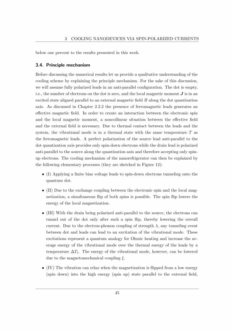
3 COOLING NANODEVICES VIA SPIN-POLARIZED CURRENTS
below one percent to the results presented in this work.
3.4. Principle mechanism
Before discussing the numerical results let us provide a qualitative understanding of the
cooling scheme by explaining the principle mechanism. For the sake of this discussion,
we will assume fully polarized leads in an anti-parallel configuration. The dot is empty,
i.e., the number of electrons on the dot is zero, and the local magnetic moment J is in an
excited state aligned parallel to an external magnetic field B along the dot quantization
axis. As discussed in Chapter 2.2.2 the presence of ferromagnetic leads generates an
effective magnetic field. In order to create an interaction between the electronic spin
and the local magnetic moment, a noncollinear situation between the effective field
and the external field is necessary. Due to thermal contact between the leads and the
system, the vibrational mode is in a thermal state with the same temperature T as
the ferromagnetic leads. A perfect polarization of the source lead anti-parallel to the
dot quantization axis provides only spin-down electrons while the drain lead is polarized
anti-parallel to the source along the quantization axis and therefore accepting only spin-
up electrons. The cooling mechanism of the nanorefrigerator can then be explained by
the following elementary processes (they are sketched in Figure 12):
• (I) Applying a finite bias voltage leads to spin-down electrons tunneling onto the
quantum dot.
• (II) Due to the exchange coupling between the electronic spin and the local mag-
netization, a simultaneous flip of both spins is possible. The spin flip lowers the
energy of the local magnetization.
• (III) With the drain being polarized anti-parallel to the source, the electrons can
tunnel out of the dot only after such a spin flip, thereby lowering the overall
current. Due to the electron-phonon coupling of strength λ, any tunneling event
between dot and leads can lead to an excitation of the vibrational mode. These
excitations represent a quantum analogy for Ohmic heating and increase the av-
erage energy of the vibrational mode over the thermal energy of the leads by a
temperature ∆T1. The energy of the vibrational mode, however, can be lowered
due to the magnetomechanical coupling ξ.
• (IV) The vibration can relax when the magnetization is flipped from a low energy
(spin down) into the high energy (spin up) state parallel to the external field,
45
3.4 Principle mechanism
Figure 12: Schematic of the elementary processes for the nanorefrigerator. (I) Tun-neling of an spin-down electron onto the quantum dot. (II) Simultaneousspin flip of electronic spin s and local magnetic moment J due to exchangecoupling q. (III) The spin-up electron can leave the quantum dot. Thetunneling process excites the vibrational mode by ∆T1. (IV) The magne-tomechanical coupling ξ induces spin flip of the local magnetic moment atthe cost of vibrational energy. The new vibrational temperature is given byTvib + ∆T1 −∆T2.
46
3 COOLING NANODEVICES VIA SPIN-POLARIZED CURRENTS
thereby reducing the vibrational temperature by ∆T2. The energy stored in the
magnetization can then again be removed by interaction with the spin of the next
tunneling electron as symbolized in (I) thus leading to a net cooling effect of the
vibrational mode.
An important component for a cooling effect is the ratio between the Ohmic heating
∆T1 induced by the electronic current and the removal of heat ∆T2 due to spin flips.
Furthermore, the polarization of the local magnetic moment by the electronic spin
plays an important role. The efficiency of the cooling protocol can therefore depend
on the lead polarization, the polarization directions, the electron-phonon coupling and
magnetomechanical coupling strengths, and the energy difference between the high- and
the low-energy spin state induced by the external field B.
3.5. Preparation
In order to be able to quantify a cooling effect, it is necessary to both define an effective
temperature for the vibrational degrees of freedom of the system as well as to prepare
the system in a suitable initial state. The stationary solution of the Markovian quantum
master equation does not depend on the initial state of the system. We are, however,
interested in the spin and the phonon dynamics of our system. The time evolution of
the density matrix explicitly depends on the initial state. While choosing an arbitrary
preparation similar to what we chose to describe the principle mechanism might yield a
meaningful time evolution, it might very well lead to misleading results with respect to
the cooling efficiency of the nanorefrigerator. Let us revise this with two extreme exam-
ples. Imagine the device to be prepared in such a way that the vibrational mode is in its
ground state. In this case, the vibrational temperature is at a minimum which makes
further cooling of the vibrational degrees of freedom impossible. Similarly, if we prepare
the system in a highly excited state we start with a high vibrational temperature. If
the initial vibrational temperature is higher than the temperature of the ferromagnetic
leads, a cooling effect will occur due to the thermal contact between the device and the
environment. This cooling effect however does not differ from the mechanism used in
passive cooling devices as mentioned previously. Our aim is to investigate the viability
of the dynamical demagnetization cooling on the nanoscale via spin-polarized currents.
A suitable preparation can be found by placing the nanodevice in thermal equilibrium
with the leads. In this way, passive cooling effects can be ruled out and a decrease of the
effective temperature below this initial preparation will show the viability of a dynamic
47
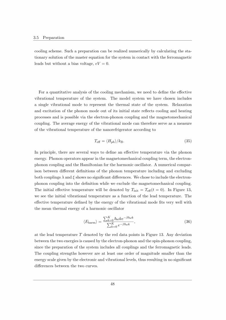
3.5 Preparation
cooling scheme. Such a preparation can be realized numerically by calculating the sta-
tionary solution of the master equation for the system in contact with the ferromagnetic
leads but without a bias voltage, eV = 0.
For a quantitative analysis of the cooling mechanism, we need to define the effective
vibrational temperature of the system. The model system we have chosen includes
a single vibrational mode to represent the thermal state of the system. Relaxation
and excitation of the phonon mode out of its initial state reflects cooling and heating
processes and is possible via the electron-phonon coupling and the magnetomechanical
coupling. The average energy of the vibrational mode can therefore serve as a measure
of the vibrational temperature of the nanorefrigerator according to
Teff = 〈Hph〉/kB. (35)
In principle, there are several ways to define an effective temperature via the phonon
energy. Phonon operators appear in the magnetomechanical coupling term, the electron-
phonon coupling and the Hamiltonian for the harmonic oscillator. A numerical compar-
ison between different definitions of the phonon temperature including and excluding
both couplings λ and ξ shows no significant differences. We chose to include the electron-
phonon coupling into the definition while we exclude the magnetomechanical coupling.
The initial effective temperature will be denoted by Tinit = Teff(t = 0). In Figure 13,
we see the initial vibrational temperature as a function of the lead temperature. The
effective temperature defined by the energy of the vibrational mode fits very well with
the mean thermal energy of a harmonic oscillator
〈Eharm〉 =
∑Kk=0 ~ωke−β~ωk∑Kk=0 e
−β~ωk, (36)
at the lead temperature T denoted by the red data points in Figure 13. Any deviation
between the two energies is caused by the electron-phonon and the spin-phonon coupling,
since the preparation of the system includes all couplings and the ferromagnetic leads.
The coupling strengths however are at least one order of magnitude smaller than the
energy scale given by the electronic and vibrational levels, thus resulting in no significant
differences between the two curves.
48
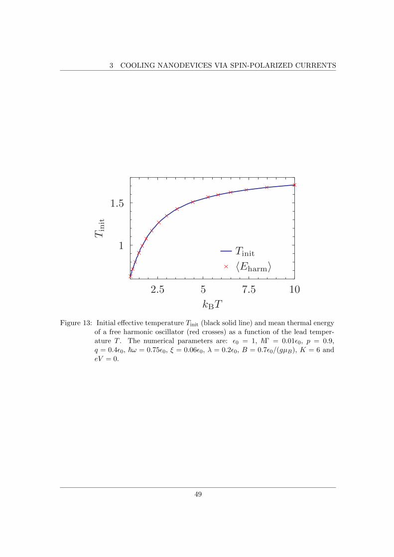
3 COOLING NANODEVICES VIA SPIN-POLARIZED CURRENTS
2.5 5 7.5 10
kBT
1
1.5
Tinit
Tinit
〈Eharm〉
Figure 13: Initial effective temperature Tinit (black solid line) and mean thermal energyof a free harmonic oscillator (red crosses) as a function of the lead temper-ature T . The numerical parameters are: ε0 = 1, ~Γ = 0.01ε0, p = 0.9,q = 0.4ε0, ~ω = 0.75ε0, ξ = 0.06ε0, λ = 0.2ε0, B = 0.7ε0/(gµB), K = 6 andeV = 0.
49
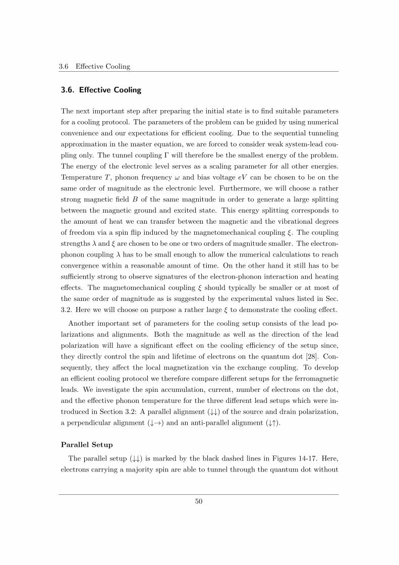
3.6 Effective Cooling
3.6. Effective Cooling
The next important step after preparing the initial state is to find suitable parameters
for a cooling protocol. The parameters of the problem can be guided by using numerical
convenience and our expectations for efficient cooling. Due to the sequential tunneling
approximation in the master equation, we are forced to consider weak system-lead cou-
pling only. The tunnel coupling Γ will therefore be the smallest energy of the problem.
The energy of the electronic level serves as a scaling parameter for all other energies.
Temperature T , phonon frequency ω and bias voltage eV can be chosen to be on the
same order of magnitude as the electronic level. Furthermore, we will choose a rather
strong magnetic field B of the same magnitude in order to generate a large splitting
between the magnetic ground and excited state. This energy splitting corresponds to
the amount of heat we can transfer between the magnetic and the vibrational degrees
of freedom via a spin flip induced by the magnetomechanical coupling ξ. The coupling
strengths λ and ξ are chosen to be one or two orders of magnitude smaller. The electron-
phonon coupling λ has to be small enough to allow the numerical calculations to reach
convergence within a reasonable amount of time. On the other hand it still has to be
sufficiently strong to observe signatures of the electron-phonon interaction and heating
effects. The magnetomechanical coupling ξ should typically be smaller or at most of
the same order of magnitude as is suggested by the experimental values listed in Sec.
3.2. Here we will choose on purpose a rather large ξ to demonstrate the cooling effect.
Another important set of parameters for the cooling setup consists of the lead po-
larizations and alignments. Both the magnitude as well as the direction of the lead
polarization will have a significant effect on the cooling efficiency of the setup since,
they directly control the spin and lifetime of electrons on the quantum dot [28]. Con-
sequently, they affect the local magnetization via the exchange coupling. To develop
an efficient cooling protocol we therefore compare different setups for the ferromagnetic
leads. We investigate the spin accumulation, current, number of electrons on the dot,
and the effective phonon temperature for the three different lead setups which were in-
troduced in Section 3.2: A parallel alignment (↓↓) of the source and drain polarization,
a perpendicular alignment (↓→) and an anti-parallel alignment (↓↑).
Parallel Setup
The parallel setup (↓↓) is marked by the black dashed lines in Figures 14-17. Here,
electrons carrying a majority spin are able to tunnel through the quantum dot without
50
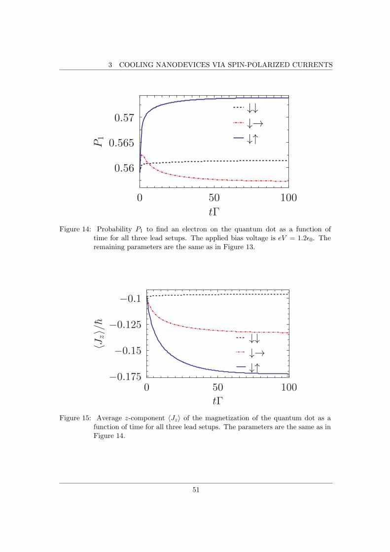
3 COOLING NANODEVICES VIA SPIN-POLARIZED CURRENTS
0 50 100
tΓ
0.56
0.565
0.57
P1
↓↓↓→↓↑
Figure 14: Probability P1 to find an electron on the quantum dot as a function oftime for all three lead setups. The applied bias voltage is eV = 1.2ε0. Theremaining parameters are the same as in Figure 13.
0 50 100
tΓ
−0.175
−0.15
−0.125
−0.1
〈Jz〉/h
↓↓↓→↓↑
Figure 15: Average z-component 〈Jz〉 of the magnetization of the quantum dot as afunction of time for all three lead setups. The parameters are the same as inFigure 14.
51

3.6 Effective Cooling
0 50 100
tΓ
0.03
0.04
0.05
〈Ih/eΓ〉
↓↓↓→↓↑
Figure 16: Charge current 〈I〉 as a function of time for three different lead setups. Theparameters are the same as in Figure 14.
0 50 100
tΓ
0.8
0.9
1
1.1
kBTeff/ǫ
0
↓↓↓→↓↑
Figure 17: Effective vibrational temperature Teff as a function of time for three differentlead setups. The parameters are the same as in Figure 14.
52
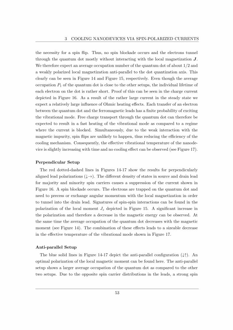
3 COOLING NANODEVICES VIA SPIN-POLARIZED CURRENTS
the necessity for a spin flip. Thus, no spin blockade occurs and the electrons tunnel
through the quantum dot mostly without interacting with the local magnetization J .
We therefore expect an average occupation number of the quantum dot of about 1/2 and
a weakly polarized local magnetization anti-parallel to the dot quantization axis. This
clearly can be seen in Figure 14 and Figure 15, respectively. Even though the average
occupation P1 of the quantum dot is close to the other setups, the individual lifetime of
each electron on the dot is rather short. Proof of this can be seen in the charge current
depicted in Figure 16. As a result of the rather large current in the steady state we
expect a relatively large influence of Ohmic heating effects. Each transfer of an electron
between the quantum dot and the ferromagnetic leads has a finite probability of exciting
the vibrational mode. Free charge transport through the quantum dot can therefore be
expected to result in a fast heating of the vibrational mode as compared to a regime
where the current is blocked. Simultaneously, due to the weak interaction with the
magnetic impurity, spin flips are unlikely to happen, thus reducing the efficiency of the
cooling mechanism. Consequently, the effective vibrational temperature of the nanode-
vice is slightly increasing with time and no cooling effect can be observed (see Figure 17).
Perpendicular Setup
The red dotted-dashed lines in Figures 14-17 show the results for perpendicularly
aligned lead polarizations (↓→). The different density of states in source and drain lead
for majority and minority spin carriers causes a suppression of the current shown in
Figure 16. A spin blockade occurs. The electrons are trapped on the quantum dot and
need to precess or exchange angular momentum with the local magnetization in order
to tunnel into the drain lead. Signatures of spin-spin interactions can be found in the
polarization of the local moment Jz depicted in Figure 15. A significant increase in
the polarization and therefore a decrease in the magnetic energy can be observed. At
the same time the average occupation of the quantum dot decreases with the magnetic
moment (see Figure 14). The combination of these effects leads to a sizeable decrease
in the effective temperature of the vibrational mode shown in Figure 17.
Anti-parallel Setup
The blue solid lines in Figure 14-17 depict the anti-parallel configuration (↓↑). An
optimal polarization of the local magnetic moment can be found here. The anti-parallel
setup shows a larger average occupation of the quantum dot as compared to the other
two setups. Due to the opposite spin carrier distributions in the leads, a strong spin
53
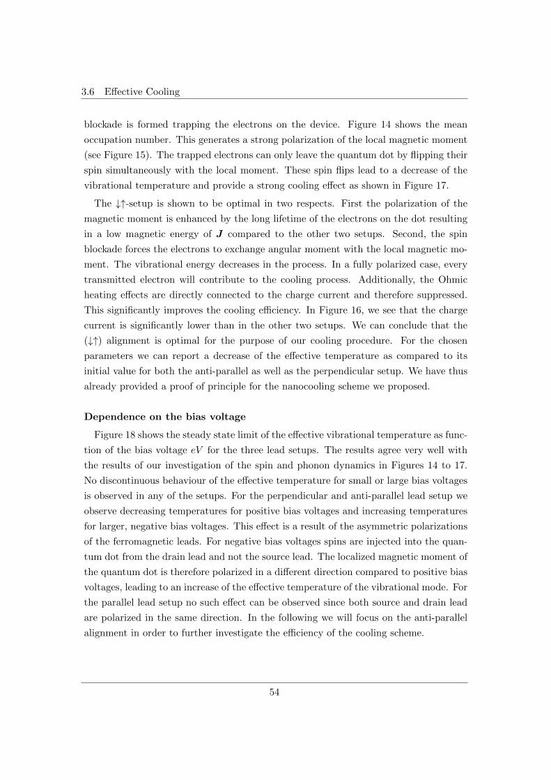
3.6 Effective Cooling
blockade is formed trapping the electrons on the device. Figure 14 shows the mean
occupation number. This generates a strong polarization of the local magnetic moment
(see Figure 15). The trapped electrons can only leave the quantum dot by flipping their
spin simultaneously with the local moment. These spin flips lead to a decrease of the
vibrational temperature and provide a strong cooling effect as shown in Figure 17.
The ↓↑-setup is shown to be optimal in two respects. First the polarization of the
magnetic moment is enhanced by the long lifetime of the electrons on the dot resulting
in a low magnetic energy of J compared to the other two setups. Second, the spin
blockade forces the electrons to exchange angular moment with the local magnetic mo-
ment. The vibrational energy decreases in the process. In a fully polarized case, every
transmitted electron will contribute to the cooling process. Additionally, the Ohmic
heating effects are directly connected to the charge current and therefore suppressed.
This significantly improves the cooling efficiency. In Figure 16, we see that the charge
current is significantly lower than in the other two setups. We can conclude that the
(↓↑) alignment is optimal for the purpose of our cooling procedure. For the chosen
parameters we can report a decrease of the effective temperature as compared to its
initial value for both the anti-parallel as well as the perpendicular setup. We have thus
already provided a proof of principle for the nanocooling scheme we proposed.
Dependence on the bias voltage
Figure 18 shows the steady state limit of the effective vibrational temperature as func-
tion of the bias voltage eV for the three lead setups. The results agree very well with
the results of our investigation of the spin and phonon dynamics in Figures 14 to 17.
No discontinuous behaviour of the effective temperature for small or large bias voltages
is observed in any of the setups. For the perpendicular and anti-parallel lead setup we
observe decreasing temperatures for positive bias voltages and increasing temperatures
for larger, negative bias voltages. This effect is a result of the asymmetric polarizations
of the ferromagnetic leads. For negative bias voltages spins are injected into the quan-
tum dot from the drain lead and not the source lead. The localized magnetic moment of
the quantum dot is therefore polarized in a different direction compared to positive bias
voltages, leading to an increase of the effective temperature of the vibrational mode. For
the parallel lead setup no such effect can be observed since both source and drain lead
are polarized in the same direction. In the following we will focus on the anti-parallel
alignment in order to further investigate the efficiency of the cooling scheme.
54
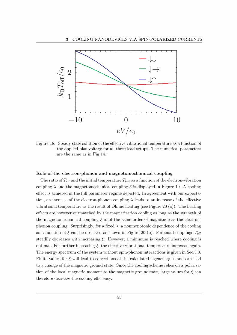
3 COOLING NANODEVICES VIA SPIN-POLARIZED CURRENTS
−10 0 10
eV/ǫ0
1
2
kBTeff/ǫ
0↓↓↓→↓↑
Figure 18: Steady state solution of the effective vibrational temperature as a function ofthe applied bias voltage for all three lead setups. The numerical parametersare the same as in Fig 14.
Role of the electron-phonon and magnetomechamical coupling
The ratio of Teff and the initial temperature Tinit as a function of the electron-vibration
coupling λ and the magnetomechanical coupling ξ is displayed in Figure 19. A cooling
effect is achieved in the full parameter regime depicted. In agreement with our expecta-
tion, an increase of the electron-phonon coupling λ leads to an increase of the effective
vibrational temperature as the result of Ohmic heating (see Figure 20 (a)). The heating
effects are however outmatched by the magnetization cooling as long as the strength of
the magnetomechanical coupling ξ is of the same order of magnitude as the electron-
phonon coupling. Surprisingly, for a fixed λ, a nonmonotonic dependence of the cooling
as a function of ξ can be observed as shown in Figure 20 (b). For small couplings Teff
steadily decreases with increasing ξ. However, a minimum is reached where cooling is
optimal. For further increasing ξ, the effective vibrational temperature increases again.
The energy spectrum of the system without spin-phonon interactions is given in Sec.3.3.
Finite values for ξ will lead to corrections of the calculated eigenenergies and can lead
to a change of the magnetic ground state. Since the cooling scheme relies on a polariza-
tion of the local magnetic moment to the magnetic groundstate, large values for ξ can
therefore decrease the cooling efficiency.
55
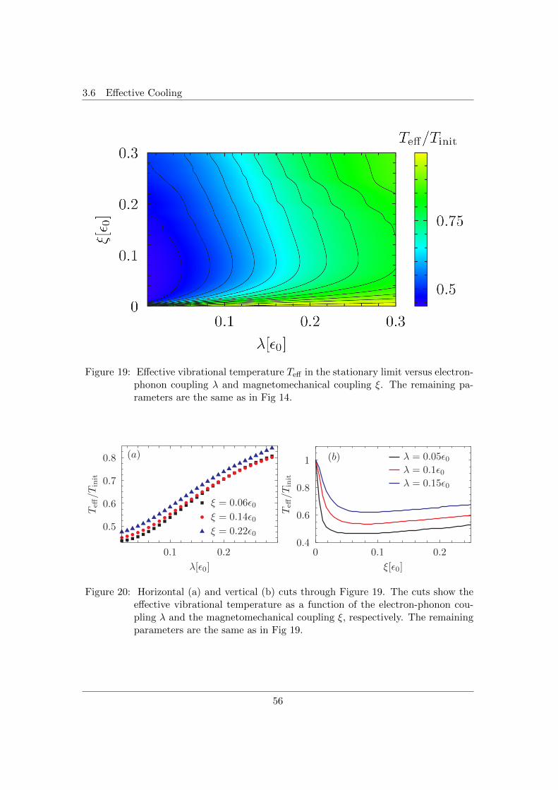
3.6 Effective Cooling
Figure 19: Effective vibrational temperature Teff in the stationary limit versus electron-phonon coupling λ and magnetomechanical coupling ξ. The remaining pa-rameters are the same as in Fig 14.
(a)
0.1 0.2
λ[ǫ0]
0.5
0.6
0.7
0.8
Teff/Tinit
ξ = 0.06ǫ0ξ = 0.14ǫ0ξ = 0.22ǫ0
(b)
0 0.1 0.2
ξ[ǫ0]
0.4
0.6
0.8
1
Teff/T
init
λ = 0.05ǫ0λ = 0.1ǫ0λ = 0.15ǫ0
Figure 20: Horizontal (a) and vertical (b) cuts through Figure 19. The cuts show theeffective vibrational temperature as a function of the electron-phonon cou-pling λ and the magnetomechanical coupling ξ, respectively. The remainingparameters are the same as in Fig 19.
56
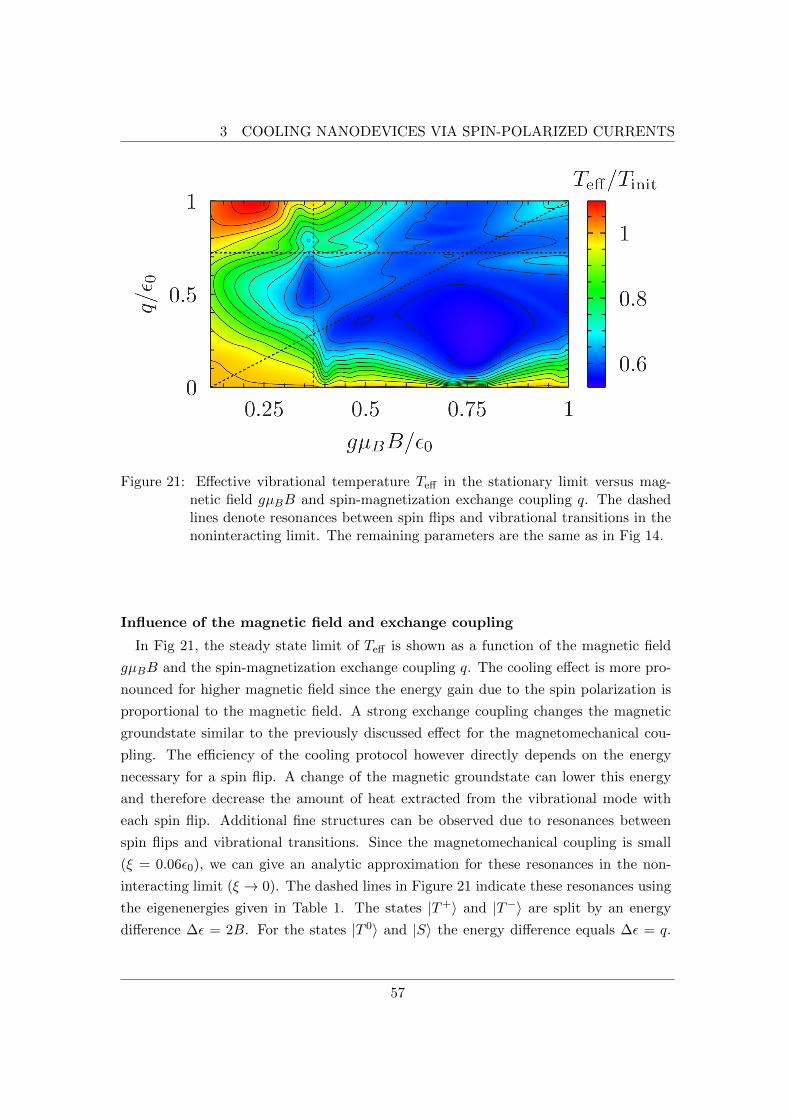
3 COOLING NANODEVICES VIA SPIN-POLARIZED CURRENTS
Figure 21: Effective vibrational temperature Teff in the stationary limit versus mag-netic field gµBB and spin-magnetization exchange coupling q. The dashedlines denote resonances between spin flips and vibrational transitions in thenoninteracting limit. The remaining parameters are the same as in Fig 14.
Influence of the magnetic field and exchange coupling
In Fig 21, the steady state limit of Teff is shown as a function of the magnetic field
gµBB and the spin-magnetization exchange coupling q. The cooling effect is more pro-
nounced for higher magnetic field since the energy gain due to the spin polarization is
proportional to the magnetic field. A strong exchange coupling changes the magnetic
groundstate similar to the previously discussed effect for the magnetomechanical cou-
pling. The efficiency of the cooling protocol however directly depends on the energy
necessary for a spin flip. A change of the magnetic groundstate can lower this energy
and therefore decrease the amount of heat extracted from the vibrational mode with
each spin flip. Additional fine structures can be observed due to resonances between
spin flips and vibrational transitions. Since the magnetomechanical coupling is small
(ξ = 0.06ε0), we can give an analytic approximation for these resonances in the non-
interacting limit (ξ → 0). The dashed lines in Figure 21 indicate these resonances using
the eigenenergies given in Table 1. The states |T+〉 and |T−〉 are split by an energy
difference ∆ε = 2B. For the states |T 0〉 and |S〉 the energy difference equals ∆ε = q.
57
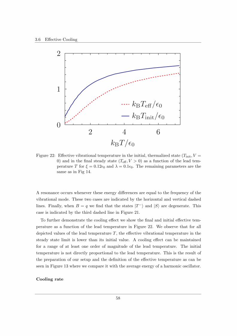
3.6 Effective Cooling
2 4 6
kBT/ǫ0
0
1
2
kBTeff/ǫ0
kBTinit/ǫ0
Figure 22: Effective vibrational temperature in the initial, thermalized state (Tinit, V =0) and in the final steady state (Teff , V > 0) as a function of the lead tem-perature T for ξ = 0.12ε0 and λ = 0.1ε0. The remaining parameters are thesame as in Fig 14.
A resonance occurs whenever these energy differences are equal to the frequency of the
vibrational mode. These two cases are indicated by the horizontal and vertical dashed
lines. Finally, when B = q we find that the states |T−〉 and |S〉 are degenerate. This
case is indicated by the third dashed line in Figure 21.
To further demonstrate the cooling effect we show the final and initial effective tem-
perature as a function of the lead temperature in Figure 22. We observe that for all
depicted values of the lead temperature T , the effective vibrational temperature in the
steady state limit is lower than its initial value. A cooling effect can be maintained
for a range of at least one order of magnitude of the lead temperature. The initial
temperature is not directly proportional to the lead temperature. This is the result of
the preparation of our setup and the definition of the effective temperature as can be
seen in Figure 13 where we compare it with the average energy of a harmonic oscillator.
Cooling rate
58

3 COOLING NANODEVICES VIA SPIN-POLARIZED CURRENTS
0 50 100
tΓ
0.7
0.8
0.9
1
1.1kBTeff/ǫ
0λ = 0.1ǫ0λ = 0.2ǫ0λ = 0.3ǫ0
Figure 23: Effective vibrational temperature Teff versus time for different electron-phonon coupling strengths λ. The parameters are the same as in Figure14.
0.05 0.1 0.15
ξ/ǫ0
0.02
0.03
0.04
0.05
Γcool/Γ
λ = 0.1ǫ0λ = 0.2ǫ0
Figure 24: Vibrational cooling rate Γcool versus the magnetomechanical coupling ξ fortwo different electron-phonon couplings λ = 0.1ε0 and λ = 0.2ε0. The re-maining parameters are the same as in Fig 14.
59
3.6 Effective Cooling
A useful measure for the efficiency of a cooling protocol is not only the maximum
achievable cooling effect, but also the speed at which the temperature is reduced. We
can define an effective temperature as in Eq. (35) at all times. Comparing the time
evolution of the effective temperature in the anti-parallel lead setup for different values
of the electron-phonon couplings, we find an exponential approach to the steady-state
as show in Figure 23. Since the vibrational temperature (see Eq.(35)) is defined by the
average energy of the vibrational mode, it depends directly on the relaxation dynamics
of the vibrational states. In Chapter 2.3.4, we have seen that the master equation can
be solved by an exponential function. The exponent is given by the Redfield rates and
the coherent oscillations of the system. The relaxation dynamics is described by the
real part of the Redfield rates. Therefore, an exponential approach of the steady-state
solution results. An effective cooling rate Γcool can therefore be determined by a fit to
our numerical results according to
Teff(t) ' Teff(∞) + e−Γcoolt(Tinit − Teff(∞)). (37)
In Figure 24, we show the cooling rate versus the magnetomechanical coupling for two
values of the electron-vibration coupling λ. An initial strong increase of the cooling rate
with increasing ξ can be observed. However, for ξ & 0.1 the cooling rate saturates. This
result is in agreement with our remarks on the observations made in Figure 21.
Dependence on the lead polarization
Naturally the effectivity of the cooling scheme depends on the degree of polarization
of the ferromagnetic leads. In Figure 25 we show the effective temperature of the device
compared to its initial value as a function of the lead polarization p. In Figure 25 (a)
we see the results for the anti-parallel setup (↓↑) which we have used so far to induce
an injection of spin-down electrons into the nanodevice. The cooling effect scales lin-
early with the polarization of the FM leads as long as a magnetomechanical coupling is
present. As expected, there is no change in the vibrational temperature to be observed
for vanishing coupling. By reversing the polarization of the leads it is also possible to
transform the nanorefrigerator into a nanoheater as shown in (b). The source lead then
provides spin-up electrons which polarize the local magnetic moment into an excited
state. The magnetomechanical interaction can then only induce spin flips which lower
the magnetic energy. The excess energy of such a process is then transferred into the
vibrational mode which leads to an increase of the effective temperature.
60
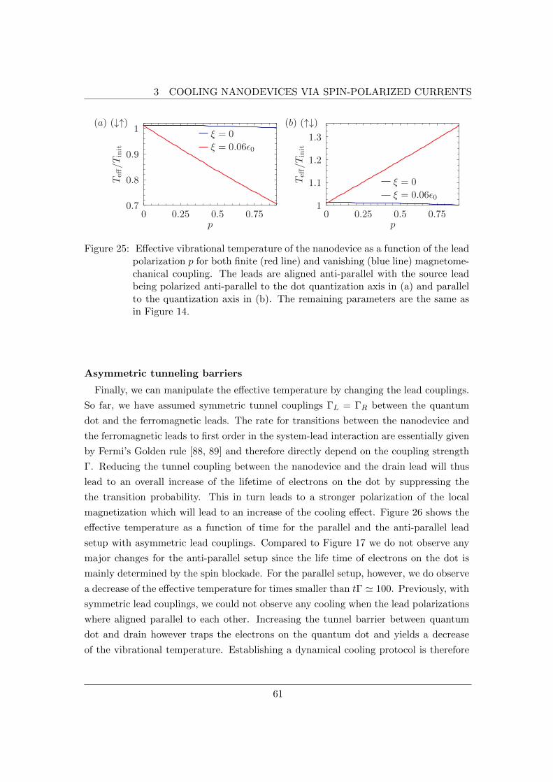
3 COOLING NANODEVICES VIA SPIN-POLARIZED CURRENTS
(a) (↓↑)
0 0.25 0.5 0.75p
0.7
0.8
0.9
1
Teff/T
init
ξ = 0
ξ = 0.06ǫ0
(b) (↑↓)
0 0.25 0.5 0.75p
1
1.1
1.2
1.3
Teff/T
init
ξ = 0
ξ = 0.06ǫ0
Figure 25: Effective vibrational temperature of the nanodevice as a function of the leadpolarization p for both finite (red line) and vanishing (blue line) magnetome-chanical coupling. The leads are aligned anti-parallel with the source leadbeing polarized anti-parallel to the dot quantization axis in (a) and parallelto the quantization axis in (b). The remaining parameters are the same asin Figure 14.
Asymmetric tunneling barriers
Finally, we can manipulate the effective temperature by changing the lead couplings.
So far, we have assumed symmetric tunnel couplings ΓL = ΓR between the quantum
dot and the ferromagnetic leads. The rate for transitions between the nanodevice and
the ferromagnetic leads to first order in the system-lead interaction are essentially given
by Fermi’s Golden rule [88, 89] and therefore directly depend on the coupling strength
Γ. Reducing the tunnel coupling between the nanodevice and the drain lead will thus
lead to an overall increase of the lifetime of electrons on the dot by suppressing the
the transition probability. This in turn leads to a stronger polarization of the local
magnetization which will lead to an increase of the cooling effect. Figure 26 shows the
effective temperature as a function of time for the parallel and the anti-parallel lead
setup with asymmetric lead couplings. Compared to Figure 17 we do not observe any
major changes for the anti-parallel setup since the life time of electrons on the dot is
mainly determined by the spin blockade. For the parallel setup, however, we do observe
a decrease of the effective temperature for times smaller than tΓ ' 100. Previously, with
symmetric lead couplings, we could not observe any cooling when the lead polarizations
where aligned parallel to each other. Increasing the tunnel barrier between quantum
dot and drain however traps the electrons on the quantum dot and yields a decrease
of the vibrational temperature. Establishing a dynamical cooling protocol is therefore
61
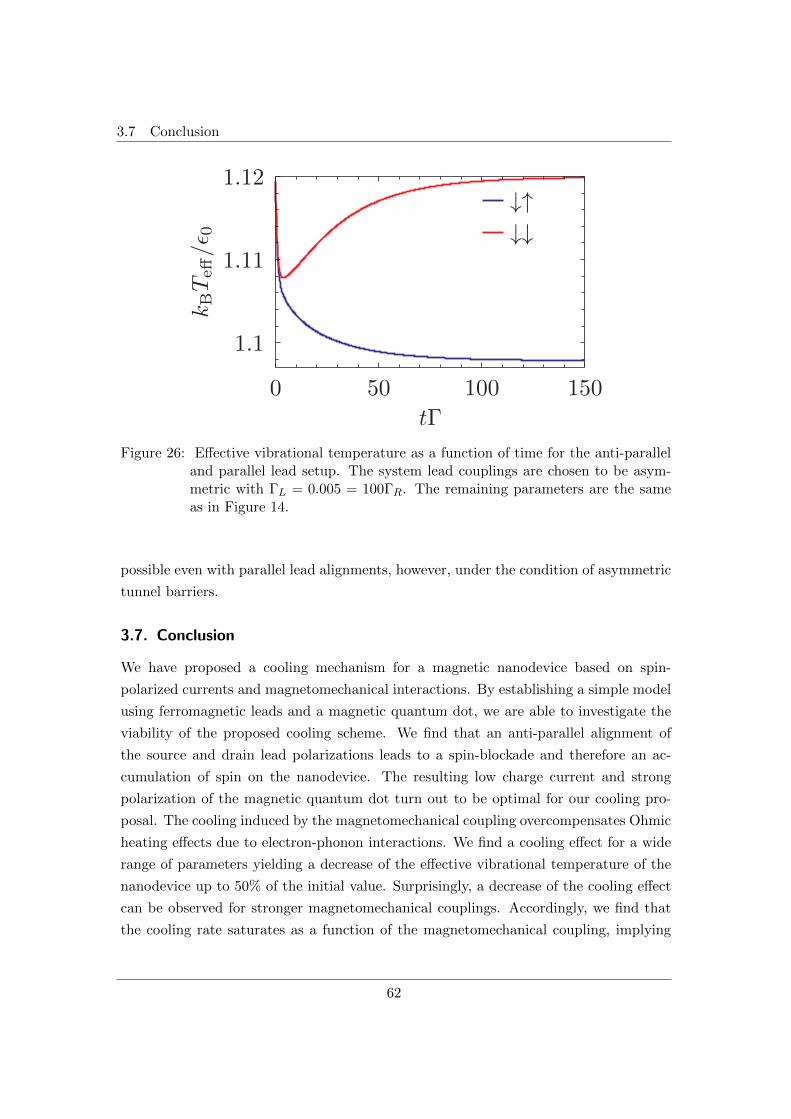
3.7 Conclusion
0 50 100 150
tΓ
1.1
1.11
1.12kBTeff/ǫ
0↓↑↓↓
Figure 26: Effective vibrational temperature as a function of time for the anti-paralleland parallel lead setup. The system lead couplings are chosen to be asym-metric with ΓL = 0.005 = 100ΓR. The remaining parameters are the sameas in Figure 14.
possible even with parallel lead alignments, however, under the condition of asymmetric
tunnel barriers.
3.7. Conclusion
We have proposed a cooling mechanism for a magnetic nanodevice based on spin-
polarized currents and magnetomechanical interactions. By establishing a simple model
using ferromagnetic leads and a magnetic quantum dot, we are able to investigate the
viability of the proposed cooling scheme. We find that an anti-parallel alignment of
the source and drain lead polarizations leads to a spin-blockade and therefore an ac-
cumulation of spin on the nanodevice. The resulting low charge current and strong
polarization of the magnetic quantum dot turn out to be optimal for our cooling pro-
posal. The cooling induced by the magnetomechanical coupling overcompensates Ohmic
heating effects due to electron-phonon interactions. We find a cooling effect for a wide
range of parameters yielding a decrease of the effective vibrational temperature of the
nanodevice up to 50% of the initial value. Surprisingly, a decrease of the cooling effect
can be observed for stronger magnetomechanical couplings. Accordingly, we find that
the cooling rate saturates as a function of the magnetomechanical coupling, implying
62
3 COOLING NANODEVICES VIA SPIN-POLARIZED CURRENTS
that not very strong couplings are required to observe the proposed effect. By reduc-
ing the strength of the tunnel coupling between the nanodevice and the drain lead a
temporary spin accumulation can be achieved even in the parallel lead configuration.
We report that, in this case, a dynamic cooling of the vibrational mode is possible with
a strong asymmetry of the tunnel couplings. Finally, be reversing the polarization of
the ferromagnetic leads, we are able to utilize the mechanism of the cooling protocol to
build a nanoheater.
63

64
4 SPIN-POLARIZED TRANSPORT THROUGH VIBRATING MOLECULES
4. Spin-polarized Transport through vibrating Molecules
Measurements of magnetic and electronic properties of molecules are often performed by
placing the sample molecule on a metal substrate. The contact with the metal substrate,
however, can lead to chemical reactions and specifically to a strong hybridization of
the sample molecule. This hybridization yields a significant change in the molecule’s
characteristics such as the orbitals, i.e., the energy spectrum, and the magnetic moment
of the molecule. If a molecule is investigated in order to determine its use as a single
molecule transistor or similar nanodevice we are, however, interested in learning the
characteristics of the molecule without hybridization between the molecular electronic
states and those of the substrate. Such a situation can be achieved experimentally by
placing the sample molecule on a non-reactive surface such as a graphene layer. The
graphene layer itself can then be placed on top of a magnetic material in order to provide
a ferromagnetic charge reservoir. A setup like this has been realized by M. Bazarnik and
J. Brede at the university of Hamburg and is schematically shown in Figure 27. In the
following, we investigate this situation in terms of a theoretical model. We adress spin-
polarized transport in an Anderson-Holstein model. In Section 4.1 the experimental
setup is explained and the experimental results are discussed. On the basis of these
results and the setup, we formulate a model for the theoretical investigation in Section
4.2. A comparison between the experimental and theoretical results is made in Section
4.3. In Section 4.4, we determine the effective field induced by the ferromagnetic leads
in order to gain further insight into the experimental results. The differences between
non-equilibrium and equilibrium phonon modes are addressed in Section 4.5. Finally,
we conclude by summarizing the results in Section 4.6.
4.1. Experiment
In order to avoid a strong hybridization of a sample molecule and its underlying host
substrate as part of the experimental preparation, it is necessary to place the molecule
on a non-reactive surface. Spectroscopic methods such as the scanning tunneling mi-
croscopy can then be used to determine the electronic properties of the sample. This
is the core idea of the experiment conducted by M. Bazarnik and J. Brede. A scheme
of the experimental setup is shown in Figure 27. The sample molecule is composed of
Phthalocyanine with a single cobalt or copper atom as a metal center (see Figure 28,
left side). This molecule is suitable for an experimental investigation for several reasons.
First, it is very stable with respect to temperature allowing to conduct experiments even
65
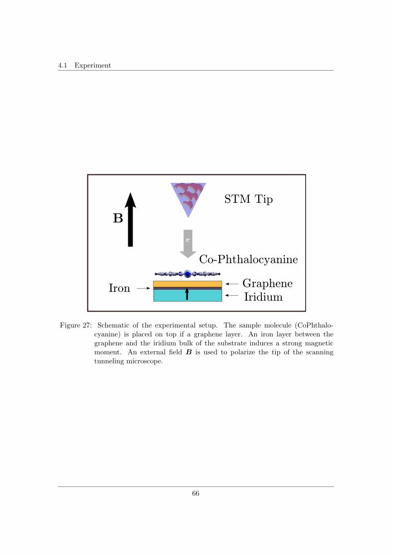
4.1 Experiment
STM Tip
Co-Phthalocyanine
GrapheneIronIridium
Figure 27: Schematic of the experimental setup. The sample molecule (CoPhthalo-cyanine) is placed on top if a graphene layer. An iron layer between thegraphene and the iridium bulk of the substrate induces a strong magneticmoment. An external field B is used to polarize the tip of the scanningtunneling microscope.
66
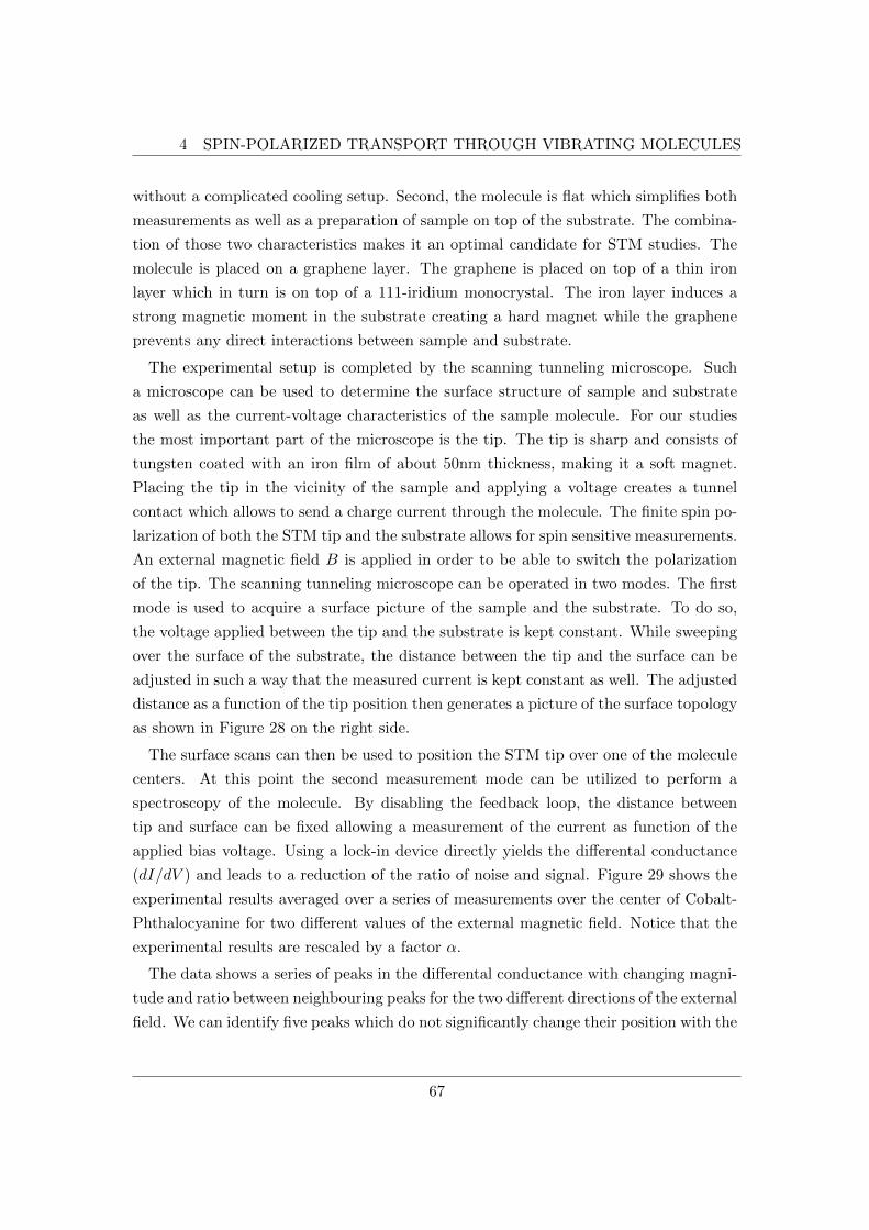
4 SPIN-POLARIZED TRANSPORT THROUGH VIBRATING MOLECULES
without a complicated cooling setup. Second, the molecule is flat which simplifies both
measurements as well as a preparation of sample on top of the substrate. The combina-
tion of those two characteristics makes it an optimal candidate for STM studies. The
molecule is placed on a graphene layer. The graphene is placed on top of a thin iron
layer which in turn is on top of a 111-iridium monocrystal. The iron layer induces a
strong magnetic moment in the substrate creating a hard magnet while the graphene
prevents any direct interactions between sample and substrate.
The experimental setup is completed by the scanning tunneling microscope. Such
a microscope can be used to determine the surface structure of sample and substrate
as well as the current-voltage characteristics of the sample molecule. For our studies
the most important part of the microscope is the tip. The tip is sharp and consists of
tungsten coated with an iron film of about 50nm thickness, making it a soft magnet.
Placing the tip in the vicinity of the sample and applying a voltage creates a tunnel
contact which allows to send a charge current through the molecule. The finite spin po-
larization of both the STM tip and the substrate allows for spin sensitive measurements.
An external magnetic field B is applied in order to be able to switch the polarization
of the tip. The scanning tunneling microscope can be operated in two modes. The first
mode is used to acquire a surface picture of the sample and the substrate. To do so,
the voltage applied between the tip and the substrate is kept constant. While sweeping
over the surface of the substrate, the distance between the tip and the surface can be
adjusted in such a way that the measured current is kept constant as well. The adjusted
distance as a function of the tip position then generates a picture of the surface topology
as shown in Figure 28 on the right side.
The surface scans can then be used to position the STM tip over one of the molecule
centers. At this point the second measurement mode can be utilized to perform a
spectroscopy of the molecule. By disabling the feedback loop, the distance between
tip and surface can be fixed allowing a measurement of the current as function of the
applied bias voltage. Using a lock-in device directly yields the differental conductance
(dI/dV ) and leads to a reduction of the ratio of noise and signal. Figure 29 shows the
experimental results averaged over a series of measurements over the center of Cobalt-
Phthalocyanine for two different values of the external magnetic field. Notice that the
experimental results are rescaled by a factor α.
The data shows a series of peaks in the differental conductance with changing magni-
tude and ratio between neighbouring peaks for the two different directions of the external
field. We can identify five peaks which do not significantly change their position with the
67
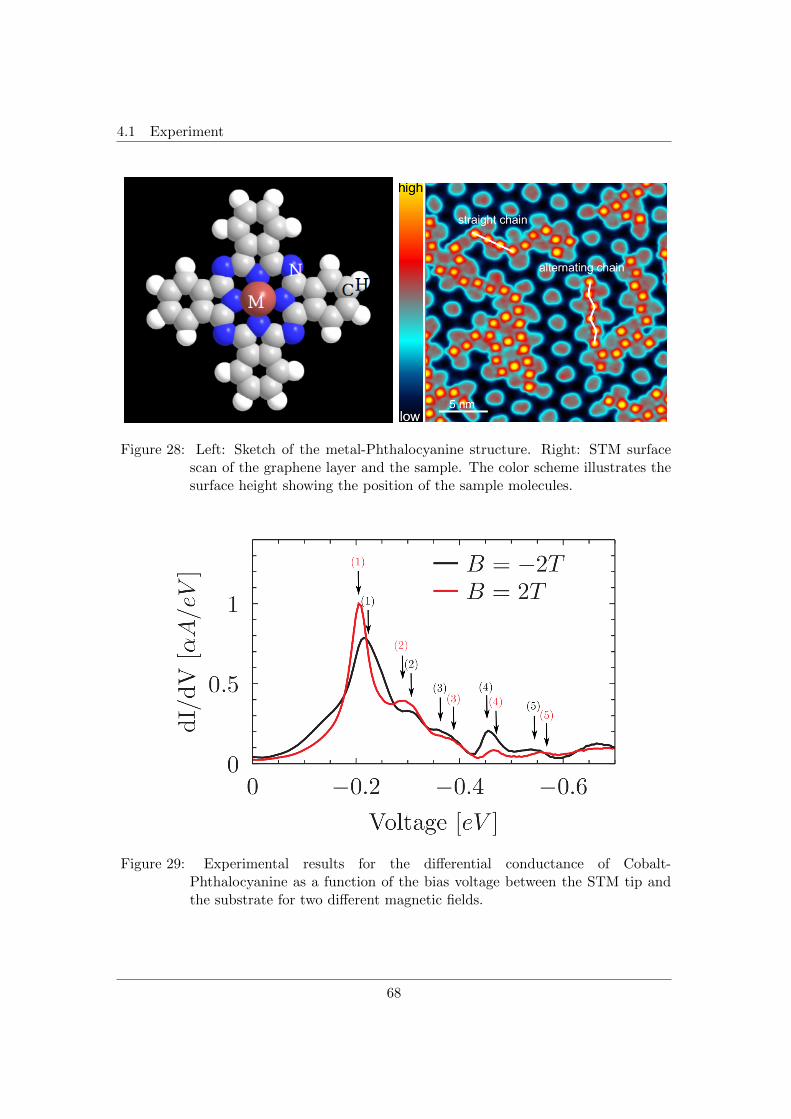
4.1 Experiment
Figure 28: Left: Sketch of the metal-Phthalocyanine structure. Right: STM surfacescan of the graphene layer and the sample. The color scheme illustrates thesurface height showing the position of the sample molecules.
Figure 29: Experimental results for the differential conductance of Cobalt-Phthalocyanine as a function of the bias voltage between the STM tip andthe substrate for two different magnetic fields.
68
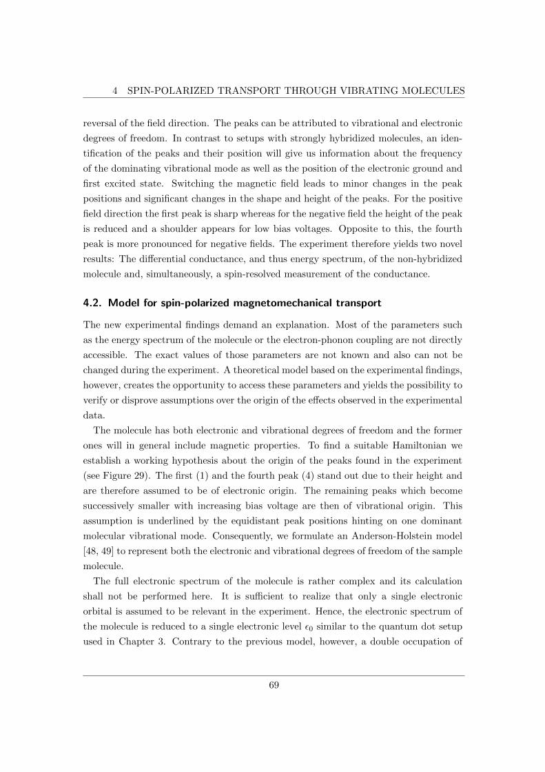
4 SPIN-POLARIZED TRANSPORT THROUGH VIBRATING MOLECULES
reversal of the field direction. The peaks can be attributed to vibrational and electronic
degrees of freedom. In contrast to setups with strongly hybridized molecules, an iden-
tification of the peaks and their position will give us information about the frequency
of the dominating vibrational mode as well as the position of the electronic ground and
first excited state. Switching the magnetic field leads to minor changes in the peak
positions and significant changes in the shape and height of the peaks. For the positive
field direction the first peak is sharp whereas for the negative field the height of the peak
is reduced and a shoulder appears for low bias voltages. Opposite to this, the fourth
peak is more pronounced for negative fields. The experiment therefore yields two novel
results: The differential conductance, and thus energy spectrum, of the non-hybridized
molecule and, simultaneously, a spin-resolved measurement of the conductance.
4.2. Model for spin-polarized magnetomechanical transport
The new experimental findings demand an explanation. Most of the parameters such
as the energy spectrum of the molecule or the electron-phonon coupling are not directly
accessible. The exact values of those parameters are not known and also can not be
changed during the experiment. A theoretical model based on the experimental findings,
however, creates the opportunity to access these parameters and yields the possibility to
verify or disprove assumptions over the origin of the effects observed in the experimental
data.
The molecule has both electronic and vibrational degrees of freedom and the former
ones will in general include magnetic properties. To find a suitable Hamiltonian we
establish a working hypothesis about the origin of the peaks found in the experiment
(see Figure 29). The first (1) and the fourth peak (4) stand out due to their height and
are therefore assumed to be of electronic origin. The remaining peaks which become
successively smaller with increasing bias voltage are then of vibrational origin. This
assumption is underlined by the equidistant peak positions hinting on one dominant
molecular vibrational mode. Consequently, we formulate an Anderson-Holstein model
[48, 49] to represent both the electronic and vibrational degrees of freedom of the sample
molecule.
The full electronic spectrum of the molecule is rather complex and its calculation
shall not be performed here. It is sufficient to realize that only a single electronic
orbital is assumed to be relevant in the experiment. Hence, the electronic spectrum of
the molecule is reduced to a single electronic level ε0 similar to the quantum dot setup
used in Chapter 3. Contrary to the previous model, however, a double occupation of
69

4.2 Model for spin-polarized magnetomechanical transport
the electronic level is in principle possible. However, the energy of double occupation is
increased by the electronic repulsion energy U . The quantum dot Hamiltonian reads
Hdot = ε0
(a†↑a↑ + a†↓a↓
)+ Ua†↑a↑a
†↓a↓ +
gµB~Bsz, (38)
where aσ is the annihilation operator for an electron with spin σ, U is the Coulomb
repulsion between two electrons on the dot, sz the electronic spin in z-direction and
B the externally applied magnetic field. Just as before, µB and g denote the Bohr
magneton and the g-factor, respectively. From the experimental results, we can extract
the frequency of the dominant vibrational mode of ω ' 0.38eV . The mode is coupled
linearly to the electronic degrees of freedom according to
Hph = ~ωb†b+ λ(b+ b†
)∑σ
a†σaσ, (39)
with b†, b denoting the phonon annihilation and creation operators and the electron-
phonon coupling strength λ. Both the STM tip and the substrate serve as electron
reservoirs and will be modelled as ferromagnetic leads. The tip will be associated with
the source lead and the substrate with the drain. In analogy with the experiment, the
drain or substrate is a hard magnet and therefore has a fixed polarization direction in
the positive z-direction. The source (or tip) polarization pL is always aligned parallel
to the external field B. Interaction between leads and sample is realized by the tunnel
coupling Hamiltonians
Htun,R =∑k
[tkR
(a↑c†k+ + a↓c
†k−
)+ h.c.
], (40)
Htun,L =∑k
[tkL
(a↑c†k± + a↓c
†k∓
)+ h.c.
], (41)
for positive/negative external fields. The tunnel amplitude for lead α is given by tkα
and the annihilation operator for electrons in the leads with wavevector k and spin σ is
given by ckσ. The Hamiltonian for the leads reads
Hleads =∑kα
(εkα − µα)(c†kα+ckα+ + c†kα−ckα−
), (42)
where εkα is the energy for lead electrons with wavevector k and µα is the chemical
potential of lead α which can be shifted by the bias voltage Vb. We choose a different
70

4 SPIN-POLARIZED TRANSPORT THROUGH VIBRATING MOLECULES
Eigenstate Energy
|0n〉 ε0n = ~ωn| ↑ n〉 ε↑n = ε0 − λ2/ω +B/2 + ~ωn| ↓ n〉 ε↓n = ε0 − λ2/ω −B/2 + ~ωn|dn〉 εdn = 2(ε0 − λ2/ω) + U − 2λ2/ω + ~ωn
Table 2: Eigenstates and corresponding energies for the Anderson-Holstein Hamiltonianwhere n denotes the excitation of the phonon mode.
label for the bias voltage compared to the previous chapter to avoid confusion with
the measurement units for the experimental data which is given in eV . In order to
study the electron and spin dynamics, it is helpful to determine the energy spectrum
of the system. The only off-diagonal term in the system Hamiltonian is the electron-
phonon coupling. An analytic diagonalization is therefore possible using the polaron
transformation. The unitary transformation is exactly the same as for the cooling model
(see Eq.(32)). However, now we also get a shift in the energy for the doubly occupied
quantum dot. The corresponding eigenenergies are given in Table 2.
4.3. Differential conductance and magnetomechanical molecular transport
Using the quantum master equation and the diagrammatic perturbation theory, we can
now compare the experimental data to numerical calculations for our model. In order to
stay as close to the experiment as possible, we use the same parameters for our numerical
calculation as far as possible. The experiment is conducted at low temperatures of
about T = 6.5K. This leads to an inverse temperature of (kBT )−1 = β = 178.51(eV)−1.
The external magnetic field has a local strength of gµBB = 2T = 0.12 × 10⁻³eV.
The magnitude of the tunnel coupling strength Γ can be estimated from the current
values obtained in the experiment. A charge current of I = 6.1nA indicates a tunnel
coupling of ~Γ ∼ 0.6 × 10⁻⁵eV . All other parameters can not be directly taken or
measured from the experiment. The polaron-shifted energy of the electronic level ε =
ε0 − λ2/ω, the Coulomb repulsion and the phonon frequency are contained in the peak
positions of the differential conductance (see Figure 29). The strength of the electron-
phonon coupling can then be estimated by fitting the theory results to the experimental
curve. A comparison between the experimental and numerical data for the differential
conductance as function of the applied bias voltage is shown for positive and negative
values of the external magnetic field in Figure 30 and Figure 31, respectively.
71
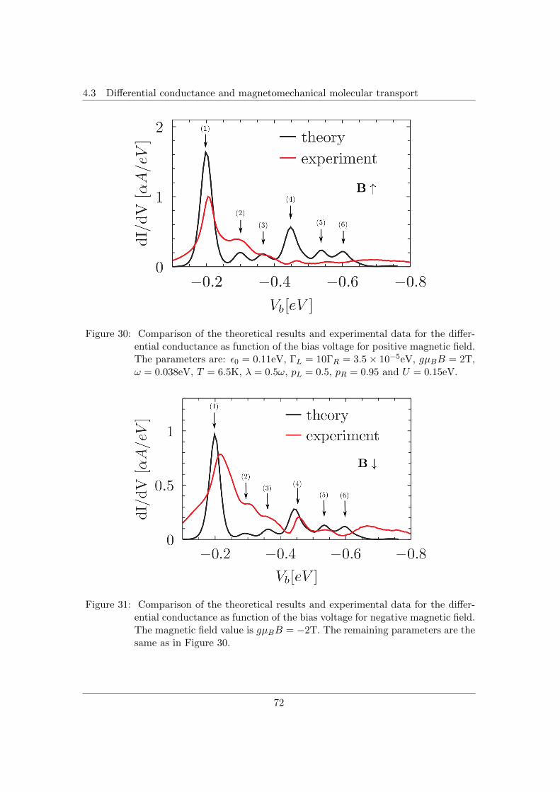
4.3 Differential conductance and magnetomechanical molecular transport
Figure 30: Comparison of the theoretical results and experimental data for the differ-ential conductance as function of the bias voltage for positive magnetic field.The parameters are: ε0 = 0.11eV, ΓL = 10ΓR = 3.5× 10⁻⁵eV, gµBB = 2T,ω = 0.038eV, T = 6.5K, λ = 0.5ω, pL = 0.5, pR = 0.95 and U = 0.15eV.
Figure 31: Comparison of the theoretical results and experimental data for the differ-ential conductance as function of the bias voltage for negative magnetic field.The magnetic field value is gµBB = −2T. The remaining parameters are thesame as in Figure 30.
72
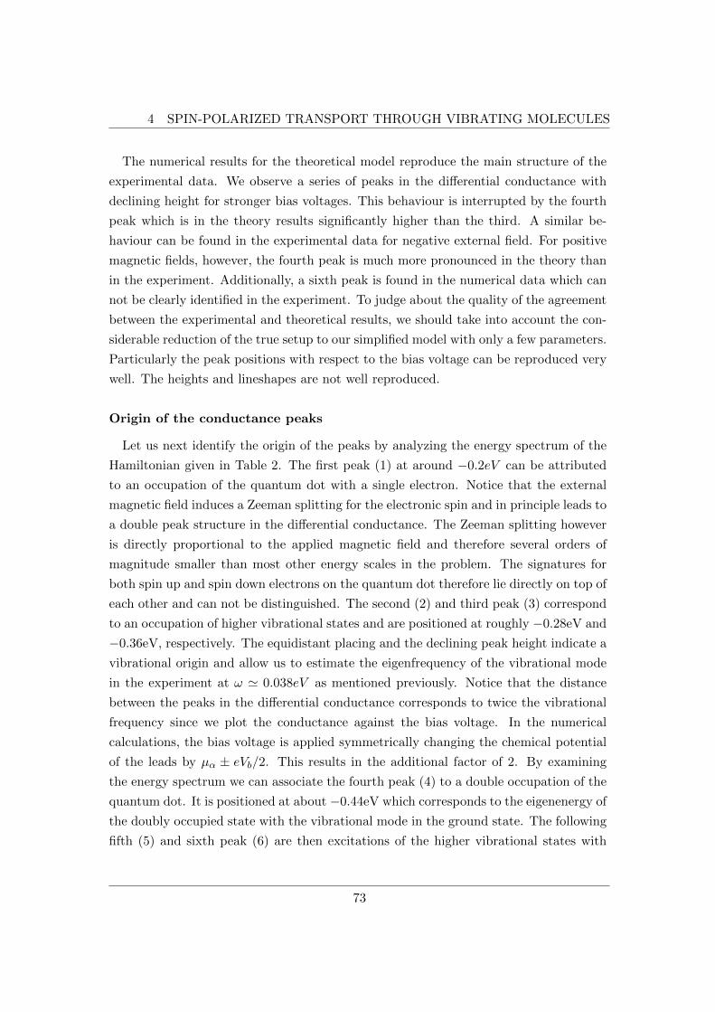
4 SPIN-POLARIZED TRANSPORT THROUGH VIBRATING MOLECULES
The numerical results for the theoretical model reproduce the main structure of the
experimental data. We observe a series of peaks in the differential conductance with
declining height for stronger bias voltages. This behaviour is interrupted by the fourth
peak which is in the theory results significantly higher than the third. A similar be-
haviour can be found in the experimental data for negative external field. For positive
magnetic fields, however, the fourth peak is much more pronounced in the theory than
in the experiment. Additionally, a sixth peak is found in the numerical data which can
not be clearly identified in the experiment. To judge about the quality of the agreement
between the experimental and theoretical results, we should take into account the con-
siderable reduction of the true setup to our simplified model with only a few parameters.
Particularly the peak positions with respect to the bias voltage can be reproduced very
well. The heights and lineshapes are not well reproduced.
Origin of the conductance peaks
Let us next identify the origin of the peaks by analyzing the energy spectrum of the
Hamiltonian given in Table 2. The first peak (1) at around −0.2eV can be attributed
to an occupation of the quantum dot with a single electron. Notice that the external
magnetic field induces a Zeeman splitting for the electronic spin and in principle leads to
a double peak structure in the differential conductance. The Zeeman splitting however
is directly proportional to the applied magnetic field and therefore several orders of
magnitude smaller than most other energy scales in the problem. The signatures for
both spin up and spin down electrons on the quantum dot therefore lie directly on top of
each other and can not be distinguished. The second (2) and third peak (3) correspond
to an occupation of higher vibrational states and are positioned at roughly −0.28eV and
−0.36eV, respectively. The equidistant placing and the declining peak height indicate a
vibrational origin and allow us to estimate the eigenfrequency of the vibrational mode
in the experiment at ω ' 0.038eV as mentioned previously. Notice that the distance
between the peaks in the differential conductance corresponds to twice the vibrational
frequency since we plot the conductance against the bias voltage. In the numerical
calculations, the bias voltage is applied symmetrically changing the chemical potential
of the leads by µα ± eVb/2. This results in the additional factor of 2. By examining
the energy spectrum we can associate the fourth peak (4) to a double occupation of the
quantum dot. It is positioned at about −0.44eV which corresponds to the eigenenergy of
the doubly occupied state with the vibrational mode in the ground state. The following
fifth (5) and sixth peak (6) are then excitations of the higher vibrational states with
73
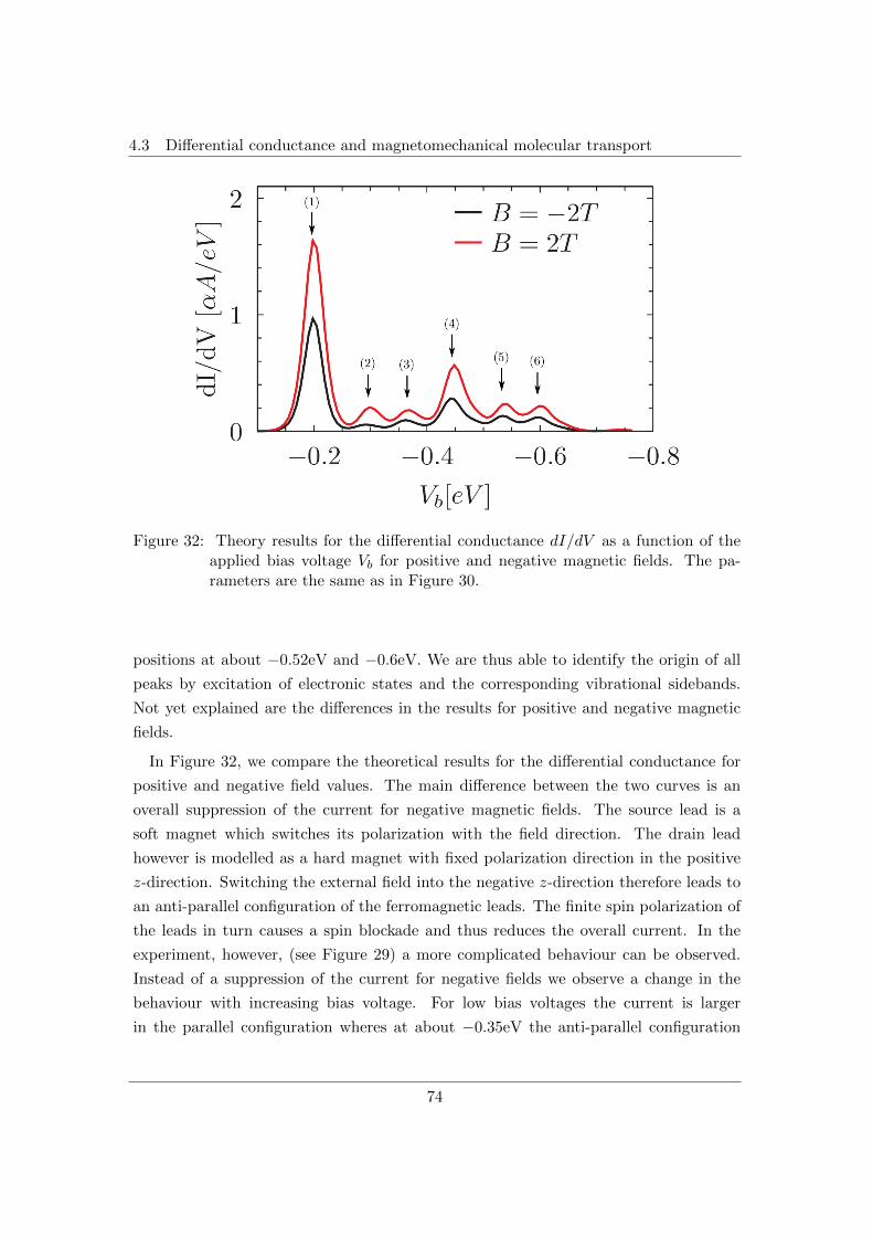
4.3 Differential conductance and magnetomechanical molecular transport
Figure 32: Theory results for the differential conductance dI/dV as a function of theapplied bias voltage Vb for positive and negative magnetic fields. The pa-rameters are the same as in Figure 30.
positions at about −0.52eV and −0.6eV. We are thus able to identify the origin of all
peaks by excitation of electronic states and the corresponding vibrational sidebands.
Not yet explained are the differences in the results for positive and negative magnetic
fields.
In Figure 32, we compare the theoretical results for the differential conductance for
positive and negative field values. The main difference between the two curves is an
overall suppression of the current for negative magnetic fields. The source lead is a
soft magnet which switches its polarization with the field direction. The drain lead
however is modelled as a hard magnet with fixed polarization direction in the positive
z-direction. Switching the external field into the negative z-direction therefore leads to
an anti-parallel configuration of the ferromagnetic leads. The finite spin polarization of
the leads in turn causes a spin blockade and thus reduces the overall current. In the
experiment, however, (see Figure 29) a more complicated behaviour can be observed.
Instead of a suppression of the current for negative fields we observe a change in the
behaviour with increasing bias voltage. For low bias voltages the current is larger
in the parallel configuration wheres at about −0.35eV the anti-parallel configuration
74
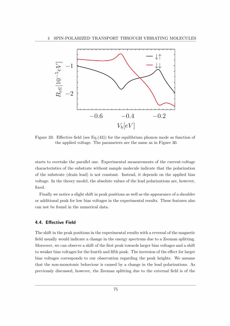
4 SPIN-POLARIZED TRANSPORT THROUGH VIBRATING MOLECULES
Figure 33: Effective field (see Eq.(43)) for the equilibrium phonon mode as function ofthe applied voltage. The parameters are the same as in Figure 30.
starts to overtake the parallel one. Experimental measurements of the current-voltage
characteristics of the substrate without sample molecule indicate that the polarization
of the substrate (drain lead) is not constant. Instead, it depends on the applied bias
voltage. In the theory model, the absolute values of the lead polarizations are, however,
fixed.
Finally we notice a slight shift in peak positions as well as the appearance of a shoulder
or additional peak for low bias voltages in the experimental results. These features also
can not be found in the numerical data.
4.4. Effective Field
The shift in the peak positions in the experimental results with a reversal of the magnetic
field usually would indicate a change in the energy spectrum due to a Zeeman splitting.
Moreover, we can observe a shift of the first peak towards larger bias voltages and a shift
to weaker bias voltages for the fourth and fifth peak. The inversion of the effect for larger
bias voltages corresponds to our observation regarding the peak heights. We assume
that the non-monotonic behaviour is caused by a change in the lead polarizations. As
previously discussed, however, the Zeeman splitting due to the external field is of the
75
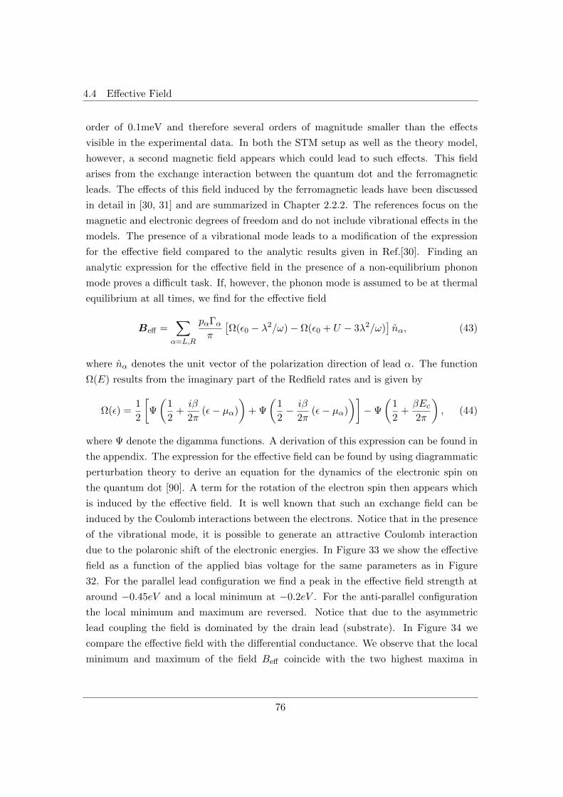
4.4 Effective Field
order of 0.1meV and therefore several orders of magnitude smaller than the effects
visible in the experimental data. In both the STM setup as well as the theory model,
however, a second magnetic field appears which could lead to such effects. This field
arises from the exchange interaction between the quantum dot and the ferromagnetic
leads. The effects of this field induced by the ferromagnetic leads have been discussed
in detail in [30, 31] and are summarized in Chapter 2.2.2. The references focus on the
magnetic and electronic degrees of freedom and do not include vibrational effects in the
models. The presence of a vibrational mode leads to a modification of the expression
for the effective field compared to the analytic results given in Ref.[30]. Finding an
analytic expression for the effective field in the presence of a non-equilibrium phonon
mode proves a difficult task. If, however, the phonon mode is assumed to be at thermal
equilibrium at all times, we find for the effective field
Beff =∑α=L,R
pαΓαπ
[Ω(ε0 − λ2/ω)− Ω(ε0 + U − 3λ2/ω)
]nα, (43)
where nα denotes the unit vector of the polarization direction of lead α. The function
Ω(E) results from the imaginary part of the Redfield rates and is given by
Ω(ε) =1
2
[Ψ
(1
2+iβ
2π(ε− µα)
)+ Ψ
(1
2− iβ
2π(ε− µα)
)]−Ψ
(1
2+βEc2π
), (44)
where Ψ denote the digamma functions. A derivation of this expression can be found in
the appendix. The expression for the effective field can be found by using diagrammatic
perturbation theory to derive an equation for the dynamics of the electronic spin on
the quantum dot [90]. A term for the rotation of the electron spin then appears which
is induced by the effective field. It is well known that such an exchange field can be
induced by the Coulomb interactions between the electrons. Notice that in the presence
of the vibrational mode, it is possible to generate an attractive Coulomb interaction
due to the polaronic shift of the electronic energies. In Figure 33 we show the effective
field as a function of the applied bias voltage for the same parameters as in Figure
32. For the parallel lead configuration we find a peak in the effective field strength at
around −0.45eV and a local minimum at −0.2eV . For the anti-parallel configuration
the local minimum and maximum are reversed. Notice that due to the asymmetric
lead coupling the field is dominated by the drain lead (substrate). In Figure 34 we
compare the effective field with the differential conductance. We observe that the local
minimum and maximum of the field Beff coincide with the two highest maxima in
76
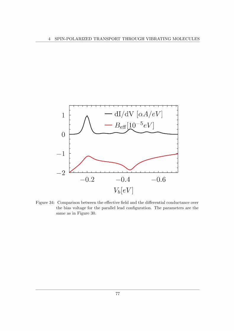
4 SPIN-POLARIZED TRANSPORT THROUGH VIBRATING MOLECULES
Figure 34: Comparison between the effective field and the differential conductance overthe bias voltage for the parallel lead configuration. The parameters are thesame as in Figure 30.
77
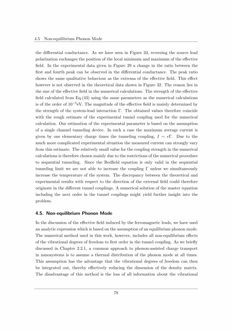
4.5 Non-equilibrium Phonon Mode
the differential conductance. As we have seen in Figure 33, reversing the source lead
polarization exchanges the position of the local minimum and maximum of the effective
field. In the experimental data given in Figure 29 a change in the ratio between the
first and fourth peak can be observed in the differential conductance. The peak ratio
shows the same qualitative behaviour as the extrema of the effective field. This effect
however is not observed in the theoretical data shown in Figure 32. The reason lies in
the size of the effective field in the numerical calculations. The strength of the effective
field calculated from Eq.(43) using the same parameters as the numerical calculations
is of the order of 10−5eV. The magnitude of the effective field is mainly determined by
the strength of the system-lead interaction Γ. The obtained values therefore coincide
with the rough estimate of the experimental tunnel coupling used for the numerical
calculation. Our estimation of the experimental parameter is based on the assumption
of a single channel tunneling device. In such a case the maximum average current is
given by one elementary charge times the tunneling coupling, I ∼ eΓ. Due to the
much more complicated experimental situation the measured current can strongly vary
from this estimate. The relatively small value for the coupling strength in the numerical
calculations is therefore chosen mainly due to the restrictions of the numerical procedure
to sequential tunneling. Since the Redfield equation is only valid in the sequential
tunneling limit we are not able to increase the coupling Γ unless we simultaneously
increase the temperature of the system. The discrepancy between the theoretical and
experimental results with respect to the direction of the external field could therefore
originate in the different tunnel couplings. A numerical solution of the master equation
including the next order in the tunnel couplings might yield further insight into the
problem.
4.5. Non-equilibrium Phonon Mode
In the discussion of the effective field induced by the ferromagnetic leads, we have used
an analytic expression which is based on the assumption of an equilibrium phonon mode.
The numerical method used in this work, however, includes all non-equilibrium effects
of the vibrational degrees of freedom to first order in the tunnel coupling. As we briefly
discussed in Chapter 2.2.1, a common approach to phonon-assisted charge transport
in nanosystems is to assume a thermal distribution of the phonon mode at all times.
This assumption has the advantage that the vibrational degrees of freedom can then
be integrated out, thereby effectively reducing the dimension of the density matrix.
The disadvantage of this method is the loss of all information about the vibrational
78
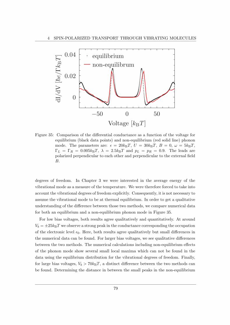
4 SPIN-POLARIZED TRANSPORT THROUGH VIBRATING MOLECULES
−50 0 50
Voltage [kBT ]
0
0.02
0.04dI/dV
[he/ΓkBT] equilibrium
non-equilibrum
Figure 35: Comparison of the differential conductance as a function of the voltage forequilibrium (black data points) and non-equilibrium (red solid line) phononmode. The parameters are: ε = 20kBT , U = 30kBT , B = 0, ω = 5kBT ,ΓL = ΓR = 0.005kBT , λ = 2.5kBT and pL = pR = 0.9. The leads arepolarized perpendicular to each other and perpendicular to the external fieldB.
degrees of freedom. In Chapter 3 we were interested in the average energy of the
vibrational mode as a measure of the temperature. We were therefore forced to take into
account the vibrational degrees of freedom explicitly. Consequently, it is not necessary to
assume the vibrational mode to be at thermal equilibrium. In order to get a qualitative
understanding of the difference between those two methods, we compare numerical data
for both an equilibrium and a non-equilibrium phonon mode in Figure 35.
For low bias voltages, both results agree qualitatively and quantitatively. At around
Vb = ±25kBT we observe a strong peak in the conductance corresponding the occupation
of the electronic level ε0. Here, both results agree qualitatively but small differences in
the numerical data can be found. For larger bias voltages, we see qualitative differences
between the two methods. The numerical calculations including non-equilibrium effects
of the phonon mode show several small local maxima which can not be found in the
data using the equilibrium distribution for the vibrational degrees of freedom. Finally,
for large bias voltages, Vb > 70kBT , a distinct difference between the two methods can
be found. Determining the distance in between the small peaks in the non-equilibrium
79
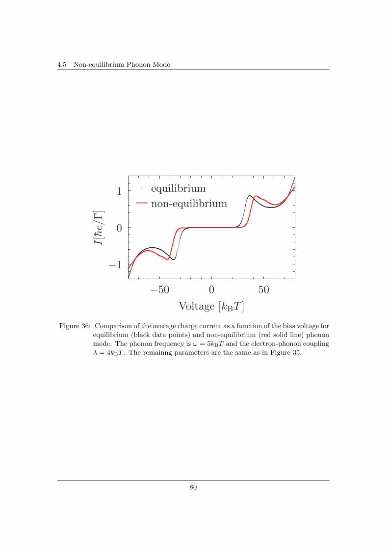
4.5 Non-equilibrium Phonon Mode
−50 0 50
Voltage [kBT ]
−1
0
1
I[he/Γ]
equilibrium
non-equilibrium
Figure 36: Comparison of the average charge current as a function of the bias voltage forequilibrium (black data points) and non-equilibrium (red solid line) phononmode. The phonon frequency is ω = 5kBT and the electron-phonon couplingλ = 4kBT . The remainng parameters are the same as in Figure 35.
80
4 SPIN-POLARIZED TRANSPORT THROUGH VIBRATING MOLECULES
results shows that the peaks are separated by an energy which corresponds to twice
the phonon frequency used for the calculation. We thus conclude that for small to
intermediate bias voltages, Vb < 50kBT , it is not necessary to consider non-equilibrium
features of the vibrational mode. For larger bias voltages, however, additional structures
appear in the differential conductance and an omission of non-equilibrium features leads
to a loss of information even for the electronic degrees of freedom. The qualitative
agreement between the two curves for bias voltages below Vb = 50kBT justifies our use
of Eq.(43) for an estimate of the influence of the ferromagnetic leads on the quantum
dot. A similar qualitative behaviour can be found in the current for stronger electron-
phonon couplings as shown in Figure 36. For a general statement about the validity of
the assumption of an equilibrium phonon mode, a more detailed comparison would be
necessary. Especially the influence of stronger electron-phonon coupling λ or different
temperatures T might play an important role. Here, the numerical calculations require a
higher number of phonon states and therefore lead to longer calculation times especially
for the non-equilibrium phonon mode. Recent calculations of the density of states of a
vibrational quantum dot in the zero-temperature limit [91] agree with our observations.
Using Monte-Carlo methods, Albrecht et. al find that the non-equilibrium distribution
of the phonons becomes important with increasing bias voltages.
4.6. Conclusion
In this chapter, we have investigated the combined effects of ferromagnetically polarized
leads and vibrational degrees of freedom on the transport through molecules. By using
an Anderson-Holstein model to describe a scanning tunneling microscopy setup, we are
able to recover most of the experimental features. A series of peaks in the differential
conductance is found in both the experimental as well as the theoretical data. We iden-
tify the origin of the conductance peaks as a combination of electronic and vibrational
states in the system and find a strong agreement between the peak positions in the
experimental data and the numerical results. New experimental results are found by
reversing the externally applied magnetic field and therefore changing the polarization
of the STM tip. The changes in the peak intensities reported in the experiment can
not be reproduced by our theoretical model. We compare the experimental data with
an analytical expression for the effective magnetic field induced by the ferromagnetic
leads. We find that, due to the numerical restriction to the sequential tunneling limit,
the signatures of this effective field can not be observed in the theory model. The qual-
itative behaviour observed in the experiment, however, indicates a interaction of the
81
4.6 Conclusion
electronic spin on the molecule with the lead polarizations. We are therefore confident
that a numerical calculation beyond the sequential tunneling limit will yield further
insight into the experimental findings. Finally, a brief comparison between equilibrium
and non-equilibrium features of the vibrational mode is made. Qualitative differences
between the two numerical results can be found in the strong bias regime where a non-
equilibrium distribution of the phonon mode leads to additional features in both the
current and conductance. We conclude that the interplay between spin-polarized charge
reservoirs and molecular vibrations yields interesting phenomena even in the absence of
a direct magnetomechanical coupling.
82
5 CONCLUSION
5. Conclusion
In this thesis we have investigated the interplay of ferromagnetic polarization of leads
with molecular vibrations. The interaction between electronic and mechanical degrees
of freedom has been widely discussed in literature. Theoretical investigation have pre-
dicted the appearance of phonon blockades of the charge transport in both strong and
weak coupling regimes which could be confirmed by experiments. The effect of spin-
polarized charge transport through molecular devices has also received attention from
both theoretical as well as experimental side. A combination of those two components
however has not been explored up to now.
We focus on two different setups presented in Chapter 3 and Chapter 4. The first de-
vice is a magnetic quantum dot coupled to noncollinear ferromagnetic leads. We show
that a polarization of the local magnetic moment of the quantum dot is possible by
utilizing spin-polarized currents. The magnetization of the quantum dot can be used to
achieve a cooling of the vibrational degrees of freedom in analogy to the macroscopic
magnetocaloric demagnetization cooling. We have developed a proof-of principle model
to determine the efficiency of the proposed cooling mechanism. The investigation of the
spin and phonon dynamics for different orientations of the lead polarizations showed
that an anti-parallel configuration of the source and drain lead polarization is optimal
with respect to the cooling efficiency. Due to the different density of states in the fer-
romagnetic leads, a spin blockade of the charge current is formed which leads to an
accumulation of spin on the quantum dot. The spin blockade reduces the inevitable
Ohmic heating caused by the charge current and an accumulation of spin yields a fast
and strong polarization of the local magnetic moment of the quantum dot. We find
that the cooling effect induced by the magnetomechanical interactions then surpasses
the Ohmic heating and a net cooling effect is achieved. A detailed investigation with
respect to the different coupling parameters reveals the possibility to decrease the ef-
fective vibrational temperature of the nanodevice by 50% compared to its initial value.
Additionally, we find an unexpected decrease of the cooling effect for stronger magne-
tomechanical couplings. Consequently, an efficient cooling setup can already be achieved
for devices with weak to intermediate magnetomechanical couplings. This behaviour is
demonstrated by a saturation of the cooling rate as a function of the magnetomechanical
interaction. By reversing the lead polarizations, we are able to transform the cooling
setup into a nanoheater. An investigation of asymmetric tunnel couplings to the leads
shows that a dynamic cooling effect can also be achieved with a parallel configuration of
83
the lead polarizations. Here, we show that the effective vibrational temperature has a
local minimum as a function of time. The asymmetric lead couplings lead to an increase
of the cooling effect for short times which is then overcome by the Ohmic heating effect
for longer times.
The second model we analyze is an Anderson-Holstein model coupled to ferromagnetic
leads. In analogy to a recent experiment we determine the differential conductance of
the Anderson dot. We find a strong agreement between the numerical and experimental
data for the position of the peaks observed in the differential conductance. We determine
that the observed structures originate from the occupation of vibronic and electronic
states of the device. A difference between the theory model and the experimental ob-
servations is found when the externally applied magnetic field and the magnetization
of the source lead are reversed. Here, the experimental data shows a change in the
peak intensities which is not reproduced by the numerical calculations. An investiga-
tion of the effective magnetic field induced by the ferromagnetic leads shows that the
strength of the magnetic interactions between leads and system is determined by the
tunnel coupling. Unlike the experimental setup, the numerical calculations performed
in this thesis are limited to the sequential tunneling limit which is valid only for weak
system-lead couplings. Consequently, the tunnel coupling chosen for the numerical cal-
culations is several orders of magnitude too small to observe a significant change in the
differential conductance as result of a field reversal. Finally, we compare the influence
of an equilibrium and a non-equilibrium phonon mode on the transport properties of
the device. For small bias voltages we observe no qualitative changes in the charge
current or conductance. At larger bias voltages, however, additional features appear in
the presence of a non-equilibrium phonon mode.
In conclusion, we find that a combination of spin-polarized transport and vibrational
degrees of freedom gives rise to interesting new phenomena. We show that, in the pres-
ence of direct magnetomechanical interactions, these effects can be used to manipulate
the thermal energy of nanodevices. Furthermore, an influence of the electron-phonon
interactions on the magnetic exchange field between the ferromagnetic leads and the
device can be found even in the absence of a direct magnetomechanical coupling.
84
A INTEGRAL KERNELS
A. Integral Kernels
In this appendix we want to take a closer look at the diagrammtic expressions for the
transition rates contained in the Redfield tensor. In Chapter 2.3.3 we have motivated the
diagrammatic rules by deriving a corresponding expression (see Eq.(21)) for the double
commutator appearing in Eq.(12). First, we determine the bath correlator Ck,α(t−t′) =
〈B†k,α(t)Bk,α(t′)〉. The bath correlator is given by the Fermi functions of the leads since
the leads are modelled as non-interacting Fermi gases,
Ck,α(t− t′) = e−iεk(t−t′)f−α (εk), (45)
where f−α (εk) =e(εk−µα)β + 1
denotes the Fermi function of lead α at temperature
T = 1/(kBβ) and chemical potential µα. Next we assume the tunnel amplitude to
be energy independent, tk,α → tα. We can then transform the sum over the lead
states in Eq.(21) into an energy integral,∑
k →∫dε. Introducing the tunnel coupling
Γα = 2π|tα|2 then yields
∫ t−∞ dt
′〈ϕ|Hint(t′)W (t)Hint(t)|ϕ〉 =
=∫ t−∞ dt
′ ∫ dε [A†(t′)A(t)ρ(t)f+α (ε)eiε(t−t
′) +A(t′)A†(t)ρ(t)f−α (ε)e−iε(t−t′)]. (46)
The next step is to perform the integrations over time and energy. First we introduce
τ = t − t′. Then we multiply by an infinitesimal factor e−ητ with η → 0. The time
integral then is of the form∫ ∞0
dxe−ηxeix(A−B) =i
A−B + iη. (47)
Solving the time integral leaves an energy integration of the type
Υ±σ (ε) =
∫ ∞−∞
dEf±α (E)
ε− E + iση, (48)
with σ = +,−. Due to the introduction of η the poles for the energy integration are
now all lifted from the real axis. In order to make the integral convergent we introduce
a Lorentzian cutoff Dα(E) = E2c
(E−µα+iEc)(E−µα−iEc) . The integral can be solved by
contour integration along half circles in the lower and upper complex plane with radius
85
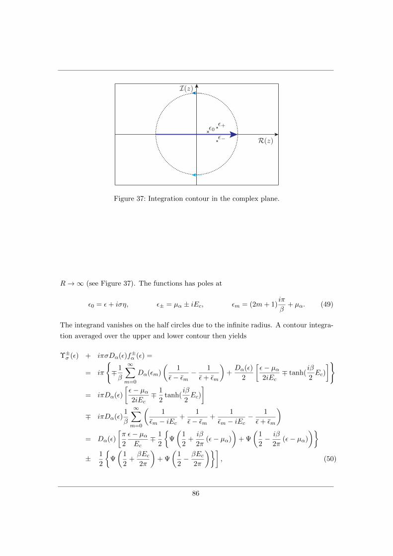
ǫ0ǫ+
ǫ− R(z)
I(z)
Figure 37: Integration contour in the complex plane.
R→∞ (see Figure 37). The functions has poles at
ε0 = ε+ iση, ε± = µα ± iEc, εm = (2m+ 1)iπ
β+ µα. (49)
The integrand vanishes on the half circles due to the infinite radius. A contour integra-
tion averaged over the upper and lower contour then yields
Υ±σ (ε) + iπσDα(ε)f±α (ε) =
= iπ
∓ 1
β
∞∑m=0
Dα(εm)
(1
ε− εm− 1
ε+ εm
)+Dα(ε)
2
[ε− µα2iEc
∓ tanh(iβ
2Ec)
]
= iπDα(ε)
[ε− µα2iEc
∓ 1
2tanh(
iβ
2Ec)
]∓ iπDα(ε)
1
β
∞∑m=0
(1
εm − iEc+
1
ε− εm+
1
εm − iEc− 1
ε+ εm
)= Dα(ε)
[π
2
ε− µαEc
∓ 1
2
Ψ
(1
2+iβ
2π(ε− µα)
)+ Ψ
(1
2− iβ
2π(ε− µα)
)± 1
2
Ψ
(1
2+βEc2π
)+ Ψ
(1
2− βEc
2π
)], (50)
86
A INTEGRAL KERNELS
where we introduced ε− µ = ε. From the first to the second line we used
Dα(εm)
[1
ε− εm− 1
ε+ εm
]=
= Dα(ε)
[1
εm + iEc+
1
ε− εm
]+Dα(ε)
[1
εm − iEc− 1
ε+ εm
]. (51)
And to evaluate the sums we exploit a property of the digamma function,
1
β
∞∑m=0
(1
εm + iEc+
1
ε− εm
)= Ψ
(1
2+iβε
2π
)−Ψ
(1
2+βEc2π
),
1
β
∞∑m=0
(1
εm − iEc− 1
ε+ εm
)= Ψ
(1
2− iβε
2π
)−Ψ
(1
2− βEc
2π
). (52)
The hyperbolic tangent can also be rewritten in terms of digamma functions:
tanh
(iβEc
2
)=
1
iπ
[Ψ
(1
2− βEc
2π
)−Ψ
(1
2+βEc2π
)]. (53)
The cutoff energy is supposed to be large, thus enabling us to approximate (50) by
Υ±σ (ε) ≈ −πiσf±α (ε)∓ Ω(ε), (54)
with
Ω(ε) =1
2
[Ψ
(1
2+iβ
2π(ε− µα)
)+ Ψ
(1
2− iβ
2π(ε− µα)
)]−Ψ
(1
2+βEc2π
). (55)
All that remains in order to determine the analytic expression for the Redfield rates
is to sum over all possible ingoing and outgoing states on the Keldysh contour and to
insert the corresponding energies of the eigenspectrum of the system.
87

88
References
References
[1] G. Moore, Electronics 38 (1965).
[2] Intel 22nm technology, http://www.intel.com/content/www/us/en/silicon-
innovations/intel-22nm-technology.html (2014).
[3] ITRS Edition Reports, http://public.itrs.net/reports.html (2010).
[4] S. Kubatkin, A. Danilov, M. Hjort, J. Cornil, J.-L. Bredas, N. Stuhr-Hansen,
P. Hedegard, and T. Bjørnholm, Nature 425, 698 (2003).
[5] H. Song, Y. Kim, Y. Jang, H. Jeong, M. A. Reed, and T. Lee, Nature 462, 1039
(2009).
[6] Y. V. Nazarov and Y. M. Blanter, Quantum Transport (Cambridge University
Press, 2009).
[7] S. Braig and K. Flensberg, Phys. Rev. B 68, 205324 (2003).
[8] J. Koch and F. von Oppen, Phys. Rev. Lett. 94, 206804 (2005).
[9] J. Koch, M. E. Raikh, and F. von Oppen, Phys. Rev. Lett. 95, 056801 (2005).
[10] M. R. Wegewijs and K. C. Nowack, New J. Phys. 7, 239 (2005).
[11] D. A. Ryndyk, M. Hartung, and G. Cuniberti, Phys. Rev. B 73, 045420 (2006).
[12] F. Pistolesi and S. Labarthe, Phys. Rev. B 76, 165317 (2007).
[13] J. Koch, M. Semmelhack, F. von Oppen, and A. Nitzan, Phys. Rev. B 73, 155306
(2006).
[14] J. Koch, F. von Oppen, and A. V. Andreev, Phys. Rev. B 74, 205438 (2006).
[15] K. Flensberg, Phys. Rev. B 68, 205323 (2003).
[16] G. Steele, A. Huttel, B. Witkamp, M. Poot, H. Meerwaldt, L. Kouwenhoven, and
H. van der Zant, Science 325, 1103 (2009).
[17] B. Lassagne, Y. Tarakanov, J. Kinaret, D. Garcia-Sanchez, and A. Bachtold, Sci-
ence 325, 1107 (2009).
89
References
[18] G. Weick, F. Pistolesi, E. Mariani, and F. von Oppen, Phys. Rev. B 81, 121409
(2010).
[19] G. Weick, F. von Oppen, and F. Pistolesi, Phys. Rev. B 83, 035420 (2011).
[20] J. Bruggemann, G. Weick, F. Pistolesi, and F. von Oppen, Phys. Rev. B 85, 125441
(2012).
[21] G. Weick and D. M.-A. Meyer, Phys. Rev. B 84, 125454 (2011).
[22] H. G. Craighead, Science 290, 1532 (2000).
[23] C. Li, D. Zhang, X. Liu, S. Han, T. Tang, C. Zhou, W. Fan, J. Koehne, J. Han,
M. Meyyappan, et al., Appl. Phys. Lett. 82, 645 (2003).
[24] J. E. Green, J. Wook Choi, A. Boukai, Y. Bunimovich, E. Johnston-Halperin,
E. DeIonno, Y. Luo, B. A. Sheriff, K. Xu, Y. Shik Shin, et al., Nature 445, 414
(2007).
[25] F. Pistolesi, Y. Blanter, and I. Martin, Phys. Rev. B 78, 085127 (2008).
[26] I. Zutic, J. Fabian, and S. D. Sarma, Rev. Mod. Phys. 76, 323 (2004).
[27] J. Konig and J. Martinek, Phys. Rev. Lett. 90, 166602 (2003).
[28] M. Braun, J. Konig, and J. Martinek, Phys. Rev. B 70, 195345 (2004).
[29] M. Braun, J. Konig, and J. Martinek, Phys. Rev. B 74, 075328 (2006).
[30] B. Sothmann, J. Konig, and A. Kadigrobov, Phys. Rev. B 82, 205314 (2010).
[31] B. Sothmann and J. Konig, Phys. Rev. B 82, 245319 (2010).
[32] A. L. Efros, E. I. Rashba, and M. Rosen, Phys. Rev. Lett. 87, 206601 (2001).
[33] M. M. E. Baumgartel, M. Hell, S. Das, and M. R. Wegewijs, Phys. Rev. Lett. 107,
087202 (2011).
[34] G. E. W. Bauer, A. H. MacDonald, and S. Maekawa, Solid State Commun. 150,
459 (2010).
[35] K. Uchida, S. Takahashi, K. Harii, J. Ieda, W. Koshibae, K. Ando, S. Maekawa,
and E. Saitoh, Nature 455, 778 (2008).
90
References
[36] F. Giazotto, T. T. Heikkila, A. Luukanen, A. M. Savin, and J. P. Pekola, Rev.
Mod. Phys. 78, 217 (2012).
[37] J. T. Muhonen, M. Meschke, and J. P. Pekola, Rep. Prog. Phys. 75, 046501 (2012).
[38] J. Bruggemann, S. Weiss, P. Nalbach, and M. Thorwart, Phys. Rev. Lett. 113,
076602 (2014).
[39] P. Stadler, W. Belzig, and G. Rastelli, Phys. Rev. Lett. 113, 047201 (2014).
[40] F. Pobell, Matter and Methods at Low Temperatures (Springer, Berlin, 2007).
[41] M. Ganzhorn, S. Klyatskaya, M. Ruben, and W. Wernsdorfer, Nature Nanotech.
8, 165 (2013).
[42] O. Arcizet, V. Jacques, A. Siria, P. Poncharal, and P. Vincent, Nature Physics 7,
879 (2011).
[43] S. Kolkowitz, A. C. B. Jayich, Q. P. Unterreithmeier, S. D. Bennett, P. Rabl,
J. G. E. Harris, and M. D. Lukin, Science 335, 1603 (2012).
[44] X. H. Qiu, G. V. Nazin, and W. Ho, Phys. Rev. Lett. 92, 206102 (2004).
[45] J. Repp, G. Meyer, S. M. Stojkovic, A. Gourdon, and C. Joachim, Phys. Rev. Lett.
94, 026803 (2005).
[46] M. Bazarnik, J. Brede, R. Decker, and R. Wiesendanger, ACS Nano 7, 11341
(2013).
[47] F. Schulz, M. Ijas, R. Drost, S. K. Hamalainen, A. Harju, A. P. Seitsonen, and
P. Liljeroth, Nature Physics 11, 229 (2015).
[48] T. Holstein, Ann. Phys. 8, 325 (1959).
[49] A. C. Hewson and D. Meyer, J. Phys.: Condes. Matter 10, 196401 (2002).
[50] J. Kondo, Prog. Theor. Phys. 32, 37 (1964).
[51] N. Makri and D. E. Makarov, J. Chem. Phys. 102, 4600 (1995).
[52] N. Makri and D. E. Makarov, J. Chem. Phys. 102, 4611 (1995).
[53] M. Thorwart, P. Reimann, P. Jung, and R. F. Fox, Chem. Phys. 235, 61 (1998).
91
References
[54] P. Nalbach and M. Thorwart, Phys. Rev. Lett. 103, 220401 (2009).
[55] R. P. Feynman and F. L. Vernon, Annals of Physics 24, 118 (1963).
[56] X.-Q. Li, J. Luo, Y.-G. Yang, P. Cui, and Y. Yan, Phys. Rev. B 71, 205304 (2005).
[57] J. Konig, J. Schmid, H. Schoeller, and G. Schon, Phys. Rev. B 54, 16820 (1996).
[58] J. Konig, H. Schoeller, and G. Schon, Phys. Rev. Lett. 76, 1715 (1996).
[59] A. Levy, R. Alicki, and R. Kosloff, Phys. Rev. E 85, 061126 (2012).
[60] M. A. Reed, J. N. Randall, R. J. Aggarwal, R. J. Matyi, and T. M. Moore, Phys.
Rev. Lett. 60, 535 (1988).
[61] B. Weber, Y. H. M. Tan, S. Mahapatra, T. F. Watson, H. Ryu, R. Rahman,
L. C. L. Hollenberg, G. Klimeck, and M. Y. Simmons, Nature Nanotechnology 9,
430 (2014).
[62] S. Amaha, W. Izumida, T. Hatano, S. Tarucha, K. Kono, and K. Ono, Phys. Rev.
B 89, 085302 (2014).
[63] C. Timm and F. Elste, Phys. Rev. B 73, 235304 (2006).
[64] F. Elste and C. Timm, Phys. Rev. B 73, 235305 (2006).
[65] U. Weiss, Quantum Dissipative Systems (World Scientific, 2008).
[66] H. Bruus and K. Flensberg, Introduction to Qauntum Field Theory in Condensed
Matter Physics (2001).
[67] C. Timm, Phys. Rev. B 77, 195416 (2008).
[68] C. Mujica-Martinez, P. Nalbach, and M. Thorwart, Phys. Rev. E 88, 062719 (2013).
[69] S. Weiss, J. Eckel, M. Thorwart, and R. Egger, Phys. Rev. B 77, 195316 (2008).
[70] C. P. Slichter, Principles of Magnetic Resonance (Springer, 1990).
[71] Y. R. Shen, The Principles of Nonlinear Optics (Wiley, 1984).
[72] C. Cohen-Tannoudji, J. Dupont-Roc, and G. Grynberg, Atom-Photon Interactions:
Basic Processes and Applications (Wiley, 1998).
92

References
[73] J. Jeske, D. Ing, M. B. Plenio, S. F. Huelga, and J. H. Cole, J. Chem. Phys. 142,
064104 (2015).
[74] R. P. Feynman, Phys. Rev. 75, 769 (1949).
[75] A. P. Jauho, Introduction to the Keldysh nonequlibrium Green function technique
(2006).
[76] G. C. Wick, Phys. Rev. 80, 268 (1950).
[77] F. Dyson, Phys. Rev. 75, 1736 (1949).
[78] D. Rugar, R. Budakian, H. Mamin, and B. Chui, Nature 430, 329 (2004).
[79] M. W. Zemansky, Temperatures very low and very high (Dover, New York, 1981).
[80] Y. Chen, C. Neill, P. Roushan, N. Leung, M. Fang, R. Barends, J. Kelly, B. Camp-
bell, Z. Chen, B. Chiaro, et al., Phys. Rev. Lett. 113, 220502 (2014).
[81] I. Bargatin and M. L. Roukes, Phys. Rev. Lett. 91, 138302 (2003).
[82] P. Rabl, P. Cappellaro, M. V. G. Dutt, L. Jiang, J. R. Maze, and M. D. Lukin,
Phys. Rev. B 79, 041302 (2009).
[83] A. A. Kovalev, L. X. Hayden, G. E. W. Bauer, and Y. Tserkovnyak, Phys. Rev.
Lett. 106, 147203 (2011).
[84] A. Palyi, P. R. Struck, M. Rudner, K. Flensberg, and G. Burkard, Phys. Rev. Lett.
108, 206811 (2012).
[85] J. Lehmann and D. Loss, Phys. Rev. B 73, 045328 (2006).
[86] J. R. Schrieffer and P. A. Wolff, Phys. Rev. 149, 491 (1966).
[87] I. G. Lang and Y. A. Firsov, Zh. Eksp. Teor. Fiz. 43, 1843 (1962).
[88] P. A. M. Dirac, Proceedings of the Royal Society A 114, 243 (1927).
[89] E. Fermi, Nuclear Physics (University of Chicago Press, 1950).
[90] S. Weiss, J. Bruggemann, and M. Thorwart, unpublished (2015).
[91] K. F. Albrecht, A. Martin-Rodero, J. Schachenmayer, and L. Muhlbacher, Phys.
Rev. B 91, 064305 (2015).
93
Danksagung
Im Folgenden mochte ich Prof. Dr. Michael Thorwart, Priv. Doz. Dr. Peter Nal-
bach und Dr. Stephan Weiss fur ihre Anleitung, Beratung, Unterstutzung und fur
ihre Geduld bei der Erstellung dieser Arbeit und der darin prasentierten Forschung
danken. Des Weiteren bedanke ich mich fur angeregte Diskussionen bei den Kollegen
aus der Forschungsgruppe Thorwart. Finanziell wurde diese Arbeit unterstutzt durch
die Deutsche Forschungsgemeinschaft (DFG) als Teil des Schwerpunktprogrammes SPP
1538 ”Spin Caloric Transport” und durch die Else-Heraeus Stiftung. Ich danke ausser-
dem meiner Familie, wo ich immer ein offenes Ohr fur meine Probleme finden konnte.
94

Eidesstaatliche Versicherung
Hiermit erklare ich an Eides statt, dass ich die vorliegende Dissertationsschrift selbst
verfasst und keine anderen als die angegebenen Quellen und Hilfsmittel benutzt habe.
Hamburg, June 12, 2015 Jochen Bruggemann
95
Publikationsliste
J. Bruggemann, S. Weiss, P. Nalbach, and M. Thorwart, Phys. Rev. Lett. 113,
076602 (2014), Cooling a Magnetic Nanoisland by Spin-Polarized Currents
96