Speed Trap or Poverty Trap?

Fines, Fees, and Financial Wellbeing∗

Steven Mello †

November 14, 2018

JOB MARKET PAPER

Please click here for most recent version

Abstract

There is widespread financial fragility in the United States and anecdotal evidencethat even small, unplanned shocks may have adverse effects on the financial situationsof fragile households. However, causal evidence on the implications of unanticipated,transitory expense shocks for low-income individuals is scarce. I study the impact offines for traffic violations on financial health, earnings and employment, and measuresof borrowing and consumption using administrative data on traffic citations in Floridalinked to high-frequency credit reports and payroll records. Leveraging variation in thetiming of traffic stops with event study and difference-in-differences research designs, Ifind that following a traffic stop, individuals experience increases in financial distress,decreases in the probability of positive payroll earnings, and reductions in measures ofconsumption and borrowing. The effects are concentrated among the poorest quartile ofdrivers, where payroll employment falls by eight percent and the increases in financialstrain induced by a $175 fine are observationally similar to what would be predictedby a $900 earnings decline. While adverse effects are partially caused by constraintson car usage due to driver license suspensions, an important mechanism appears tobe a poverty trap whereby shocks have a compounding effect for the disadvantagedpopulation. I conclude by estimating that the average traffic ticket is associated withat least a $500 welfare loss and discussing this magnitude’s implications for optimalpolicing.

∗I am grateful to Will Dobbie, Ilyana Kuziemko, David Lee, and Alex Mas for unrelenting ad-vice and encouragement on this project. Mark Aguiar, David Arnold, Reyhan Ayas, Leah Boustan,Jessica Brown, Mingyu Chen, David Cho, Felipe Goncalves, Elisa Jacome, Henrik Kleven, AndrewLangan, Atif Mian, Jack Mountjoy, Jonathan Mummolo, Chris Neilson, Scott Nelson, WhitneyRosenbaum, Mallika Thomas, Owen Zidar, and seminar participants at Princeton University pro-vided helpful comments. I thank Beth Allman for providing the citations data and for several helpfulconversations, as well as numerous individuals at the data-providing credit bureau for exceptionalassistance with accessing and working with the data. I benefitted from generous financial supportfrom the Industrial Relations Section at Princeton University, the Fellowship of Woodrow WilsonScholars, and the Charlotte Elizabeth Procter Fellowship. Any errors are my own.†Industrial Relations Section, Princeton University, Princeton, NJ 08544. smello@princeton.edu.

1 Introduction

The ability of households to cope with adverse shocks has important implications for taxa-

tion and social insurance policies (e.g., Baily 1978, Chetty 2006a). Despite the prediction of

canonical models that liquidity-constrained households anticipate income volatility by accu-

mulating buffer stock savings (Deaton 1991, Carroll 1992, Carroll 1997), recent evidence has

highlighted the lack of precautionary savings in the United States (Beshears et al., 2018).

Half of all households accumulated no savings in 2010 (Lusardi, 2011) and forty percent

of Americans indicated an inability to cover an emergency $400 expense in 2017 (Board

of Governors of the Federal Reserve System, 2018). The widespread dearth of rainy-day

funds, termed financial fragility, has spurred concern among scholars and policymakers in

recent years because fragile households may be particularly vulnerable to unexpected shocks

(Lusardi et al., 2011).

While ethnographic studies such as Shipler (2005) and Desmond (2016) are rife with

accounts of disadvantaged individuals whose fortunes are altered by unplanned expenses,

causal evidence on the impacts of transitory, negative shocks on household finances is scarce.

An important obstacle to such an empirical analysis is the lack of usable variation in small

income shocks, especially for poor households. Existing studies have examined consumption

responses to small positive shocks such as tax refunds (e.g., Parker 2017) or significant

negative shocks such as hospital admissions (Dobkin et al., 2018) or job loss (Stephens 2001,

Keys 2018). The literature’s reliance on policy variation generated by tax rebates or mortgage

programs and on credit card or bankruptcy filings data has left the bottom end of the income

distribution relatively understudied.

In this paper, I examine the impacts of fines for traffic infractions on financial wellbeing.

Over forty million traffic citations are issued each year for speed limit violations alone, mak-

ing traffic fines a common unplanned expense for the driving population. Further, policing

activity disproportionately affects poor communities, whose residents may have an especially

limited capacity to absorb fines. As shown in Figure 1, residents of the most disadvantaged

zip codes receive traffic citations at nearly twice the rate of residents of rich zip codes.1 While

1The correlation between neighborhood income and ticketing rates is consistent with a wealthof evidence suggesting that low-income and nonwhite communities tend to be the most policed. Forexample, poorer cities employ more police officers per capita (Figure A-1) and rely more heavilyon revenue from criminal justice fines and fees (Figure A-2).

1

most traffic fines are nominally small, typically between $100 and $400, they could induce

financial distress in several ways. For individuals lacking financial slack, coping mechanisms

such as forgoing basic needs, missing bills, or borrowing at high interest rates may impact

future financial stability (e.g., Skiba & Tobacman 2011). Nonpayment of fines results in

the revocation of driving privileges, which may jeopardize employment arrangements or put

individuals at risk of a misdemeanor charge for driving without a valid license.

An analysis of the impacts of fines is particularly interesting given the current public

concern regarding the unintended consequences of criminal justice policies (e.g., Ang 2018).

While a large literature has examined the public safety benefits of policing (Chalfin & Mc-

Crary, 2017) in the spirit of deterrence models such as Becker (1968), the social costs of

policing have historically received less attention. A host of recent events such as the 2014

riots in Ferguson, Missouri have vaulted the potential negative implications of policing to the

forefront of public consciousness. Prompted by the Ferguson Report ’s findings that a focus

on revenue generation shaped the city’s policing practices and that nonwhite and low-income

citizens disproportionately received citations (Department of Justice Civil Rights Division,

2015), media outlets and advocates have offered accounts of individuals suffering cycles of

debt and involvement with the criminal justice system stemming from fines and fees.2 While

compelling, such evidence is both anecdotal and correlational. To date, there has been no

rigorous empirical analysis of the causal effects of fines on economic wellbeing.

To estimate the impacts of fines, I link administrative data on the universe of traffic

citations issued in Florida over 2011–2015 to monthly credit reports and payroll records for

ticketed drivers. The citations data provide nearly complete coverage of the state’s traffic

offenders and my analysis sample represents about five percent of Florida’s driving-age popu-

lation. Credit reports offer a detailed account of an individual’s financial situation, including

information on delinquencies, adverse financial events such as charge-offs and repossessions,

and unpaid bills in collection. The payroll records report monthly earnings for individuals

working at large employers. About sixteen percent of the analysis sample is employed in a

payroll-covered job in the year prior to receiving a citation.

2For examples, see Adams (2015), Lopez (2016), Grabar (2017), or Sanchez & Kambhampati(2018). In 2015, John Oliver devoted a segment of his popular HBO show, Last Week Tonight,to municipal violations, providing several anecdotes and noting that “if you don’t have enoughmoney to pay a fine immediately, tickets can ruin your life.” See http://time.com/3754023/

john-oliver-municipal-violations/.

2

The high-frequency nature of the credit report and payroll data allows for the use of event

study and difference-in-differences research designs that leverage variation in the timing of

traffic stops for identification. My primary difference-in-differences approach compares the

evolution of outcomes for drivers around the time of a traffic stop with a matched control

group of comparable individuals who receive citations two to four years later. This empirical

strategy relies on the identifying assumption that fined drivers would have trended similarly

to control individuals in the absence of a traffic ticket, which I validate by showing that the

two groups of drivers follow parallel pre-citation trends on a host of outcomes.

First, I examine the impact of traffic fines on several measures of financial distress. In the

first year after a traffic stop, individuals experience a three percent increase in collections, a

four percent increase in collections balances, and two percent increases in delinquencies and

incidences of derogatory events. Collections activity related to an unpaid citation typically

will not appear on a credit report, so the observed increases in collections most likely reflect

increases in unpaid utility or medical bills (Avery et al., 2003). Estimated impacts persist,

and in most cases continue to grow, two years out from the traffic stop date.

For the majority of strain outcomes, treatment effects are two to five times larger for the

poorest quartile of drivers than for the richest quartile. While non-zero effect sizes for the

richest subset of drivers may seem surprising, there is evidence of widespread hand-to-mouth

behavior and binding liquidity constraints even among wealthy households (Chetty & Szeidl

2007, Kaplan et al. 2014). To help interpret the estimated magnitudes, I rely on the cross-

sectional relationship between payroll earnings and financial strain outcomes to construct

income-equivalent effect sizes — the change in income that would predict the observed change

in distress. For low-income drivers, the two-year increase in financial strain is observationally

similar to what would be predicted by a $950, or five percent, drop in earnings.

Next, I study effects on payroll outcomes. Traffic citations could affect employment status

through their impacts on financial distress, which may reduce labor supply (Dobbie & Song,

2015) or job-finding rates (Bartik & Nelson, 2017), or through their impacts on the costs

of driving. Unpaid citations result in driver license suspensions, and many tickets result in

driver license “points” which might increase auto insurance premiums. I find that one year

(two years) out from a ticket date, individuals are about three (five) percent less likely to

have any reported payroll earnings. Citations both reduce the likelihood of a transition into

a payroll-covered job and increase the likelihood of a transition out of the payroll data.

3

As with the financial strain outcomes, employment effects are most pronounced for poor

drivers. The estimated impact on payroll employment for the richest quartile of the sample

is quite small, while the poorest quartile of drivers experience nearly a ten percent decline

in the likelihood of positive reported earnings. For individuals remaining in the payroll data

following a citation, there is no effect on earnings on average, but suggestive evidence of a

two percent decline in earnings for low-income drivers.

I also examine the impact of traffic tickets on measures of borrowing and consumption. An

unplanned expense may increase demand for credit, but financial distress or unemployment

could restrict credit availability. I find small declines in the number of credit cards, credit

card balances, and the likelihood of car and home ownership, proxied by the presence of

an open auto loan and mortgage on a credit report, following a traffic stop. Reductions are

more pronounced in the long-run than the short-run, suggesting that diminished access to

credit following the accumulation of unpaid bills and delinquencies could be an important

mechanism. The pattern of heterogeneity in the borrowing effects is less stark, likely because

the poorest quartile of drivers exhibit tenuous borrowing at baseline.

After presenting the main results, I consider the relative importance of competing mech-

anisms in explaining the estimated effects. In particular, traffic tickets represent unplanned

expense shocks but also can affect insurance costs or driving privileges. Using information on

traffic ticket dispositions available for a subset of drivers, I show that treatment effects for

those whose dispositions indicate payment, and therefore typically will not incur a suspended

license, are similar to the sample-wide average effects. Impacts are smaller for individuals

making payment and electing to attend an optional traffic school that suppresses points

from accruing on the driver’s license. One the one hand, the reduced treatment effects for

school attendees suggest that the negative consequences of traffic tickets are in part due to

license suspensions or increased insurance costs (individuals making payment can still face

suspensions if payment is late or if they have accrued many past citations). On the other

hand, impacts are still present for school attendees and the treatment effect disparities are

largely eroded when accounting for observable differences between the two groups of drivers.

Further, a separate analysis reveals that the causal effects of license suspensions are large,

but not outsized compared to the main citation effects. On net, it appears that both the

pure expense shock and potential effects on driving costs are important mechanisms.

I conclude by quantifying the welfare losses associated with traffic tickets and discussing

4

policy implications. Using back-of-the-envelope calculations and a standard willingness-to-

pay framework, a conservative estimate of the welfare cost associated with the average ticket

is about $500. Intuitively, this quantity has a policy-relevant interpretation. To the extent

that welfare costs are greater than the revenue raised and public safety produced by an

additional traffic citation, there is deadweight loss associated with ticketing. Governments

who do not consider the outsized welfare costs of citations will generally choose to over-

police. I then use a simple Becker-style model to consider the welfare implications of moving

to an income-based fine system.3 In a stylized environment where individuals earn either

$20,000 or $40,000 per year and the multiplying welfare effects of fines for poor individuals

are taken into account, a $10 increase (decrease) in the fine for rich (poor) drivers yields a

welfare benefit of between $3 and $10 dollars per citation. At current ticketing levels, this

policy offers a total social benefit as high as $20 million per year, eroding about one percent

of the total welfare cost of annual citations in Florida ($500 × 2 million tickets).

My paper makes two important contributions. First, the empirical results highlight that

many individuals are not fully insured against even small economic shocks. Faced with a

$175 traffic ticket, individuals accrue unpaid bills and delinquencies on their credit reports

while also reducing consumption, suggesting an inability to cover the unexpected expense.

While the increases in unpaid bills and declines in consumption are smaller than the fine

itself for rich drivers, traffic tickets appear to have a multiplying effect on financial health

for poor drivers, who exhibit increases in financial distress observationally similar to a $950

income loss following a $175 ticket. Results are even starker for individuals with unpaid

bills at baseline, who experience the largest increases in distress and largest declines in

employment and borrowing. This pattern of results is consistent with a poverty trap (e.g.,

Banerjee & Duflo 2011, Barrett et al. 2019), whereby small shocks have minor consequences

for financially stable individuals but deleterious effects for the already distressed population.

These findings have potentially important implications for social insurance programs as

optimal policy formulas typically depend heavily on the ability of households to smooth

across states of the world. Further, the empirical analysis contributes to a large literature

studying how households are affected by economic shocks by providing some of the first

3Finland employs an income-based fine schedule for speeding. Countries such as Sweden andDenmark also use income-dependent fines in some form. See https://www.theatlantic.com/

business/archive/2015/03/finland-home-of-the-103000-speeding-ticket/387484/.

5

causal evidence on the effects of small, negative shocks for low-income individuals.4

Second, this paper adds to the current public debate over the use of fines and fees in the

criminal justice system. While scholarly work has found that increases in speeding tickets

improve road safety (Makowsky & Stratmann 2011, DeAngelo & Hansen 2014, Luca 2015),

critics have argued that the ability of police departments to raise municipal revenue through

citations distorts policing incentives (Goldstein et al., 2018). Advocates and media outlets

(e.g., Adams 2015, Lopez 2016, Grabar 2017) have argued that flat fine schedules and more

intensive policing in low-income communities result in an unfair burden of fine systems on the

poor. Others have called the harsh punishments imposed for nonpayment of fines an effective

“criminalization of poverty” (Balko, 2018). My findings illustrate the outsized impacts of fines

on the financial well-being of low-income individuals, a fact that has potentially important

implications for both the optimal level of policing and the design of fine-and-fee systems.

The remainder of the paper is organized as follows. Section 2 explains the institutional

details of traffic enforcement in Florida. I describe the data in Section 3 and the empirical

strategy in Section 4. Results are presented in Section 5. I briefly discuss welfare and policy

implications in Section 6 and conclude in Section 7.

2 Traffic Enforcement in Florida

The context of the present study is traffic enforcement in Florida. The vast majority of traffic

laws, such as speed limits, are enforced with fines for violators. Patrolling police officers, or in

some cases automated systems such as red light or toll cameras, issue citations to offenders.

Traffic tickets are very common. Over 4.5 million individual Florida drivers received at least

one traffic citation between 2011 and 2015, with between 1.1 and 1.4 million licensed Florida

drivers cited each year. As of the 2010 census, the age 18 and over population of Florida

was 14.8 million, implying that around thirty percent of the driving age population received

a citation over 2011–2015 and about seven to ten percent of the driving age population

receives a citation each year. As has been shown in other contexts, traffic enforcement appears

to disproportionately affect low-income individuals. Figure 1 illustrates a clear correlation

between the zip code ticketing rate (number of citations issued to zip code residents divided

by the zip code population) and zip code per capita income, computed from the IRS public

4Beshears et al. (2018) provides a thorough and recent review of the literature.

6

use files.5 A ten percent decline in neighborhood per capita income is associated with a four

percent increase in the citation rate.

Traffic citations specify the offense and a fine to be paid, which is determined by the

violation code and the county of the offense. For reference, the most common single violation

codes over 2011–2015 were speeding (20 percent), red light camera violations (8.5 percent),

lacking proper insurance (7.5 percent), driver not seat-belted (6 percent), and failure to pay

toll (6 percent), which account for nearly half of all citations over the period. Statutory

fines vary widely across offense types and counties. For example, in Miami-Dade county,

low-level equipment violations such as broken tail lights carry a fine of $109, while the fine

for speeding 30+ miles per hour above the posted limit in a construction or school zone

is $619. Punishments for very rare criminal, rather than civil, traffic offenses can exceed

$1,000 and in some instances may include jail time. Unfortunately, the citations database

does not include a reliable measure of the statutory fine associated with each offense. Using

an imputation procedure, I estimate that the average statutory fine faced by drivers in the

main sample is about $175, but this is likely an underestimate.

Citations can be associated with additional costs beyond the statutory fine. Traffic vio-

lations result in points on a driver’s license. Insurance companies typically consider driver-

license points when setting premiums, so individuals may face increases in car insurance

prices following a citation (Gorzelany, 2012). A rough back of the envelope calculation sug-

gests the typical speeding ticket could increase monthly car insurance premiums by $10.

State law dictates that drivers accruing 12 points in 12 months (18 points in 18 months; 24

points in 36 months) have their driver license suspended for 30 days (3 months; one year).

Most common offenses are associated with three points, but certain violations carry up to 6

points.6 Individuals cited for equipment violations such as broken taillights are ordered to

make repairs or face the risk of quickly becoming repeat offenders.

Once a citation has been issued, a driver can either submit payment to the county clerk

or request a court date to contest a ticket. For those contesting their ticket in court, a judge

or hearing officer ultimately will decide to either uphold the original citation, reduce the

punishment, or dismiss the charge. For individuals who do not request a court date, payment

5The IRS public use data are available from the IRS website at https://www.irs.gov/

statistics/soi-tax-stats-individual-income-tax-statistics-zip-code-data-soi.6See the FLDHSMV website at https://www.flhsmv.gov/driver-licenses-id-cards/

driver-license-suspensions-revocations/points-point-suspensions/.

7

is due 30 days from the citation date. At the time of payment, a driver may also elect to

attend traffic school. A voluntary traffic school election (and completion) coupled with an

on-time fine payment prevents the license points associated with the citation from accruing

on the individual’s DL.7 If the county clerk has not received payment in-full within 30 days,

the individual is considered delinquent and their license is suspended effective immediately.

Knowingly driving with a suspended license is a low-level misdemeanor offense and typically

results in a fine of $300-500 with the possibility of jail time and punishments increasing

drastically for second and third offenses.

If a citation remains unpaid after 90 days, county clerks add a late fee to the original

amount owed and send the debt to a collections agency, who then solicit payment for the

citation. Collections agencies are authorized by state law to, and therefore typically will, add

a 40 percent collection fee to the original debt.8 Relevant for the empirical analysis is whether

collections originating from unpaid citations will appear directly in the credit bureau data.

Not all collections agencies report their activity to credit bureaus and reporting behavior

varies across both agencies and clients. I compiled a list of collections agencies used by the

five largest counties in Florida by examining county clerk webpages and contacted each one

directly to inquire about their reporting behavior.9 While most signaled an ability to report

to credit bureaus on their webpage, the two agencies that responded directly to my inquiry

indicated that they did not report citation-related collections.

An important takeaway from a close examination of the institutional details is that

a traffic ticket represents a possibly multi-faceted treatment. The exact treatment for a

given individual may depend on driving history and ex post decisions, neither of which are

perfectly observed in the data. We should primarily think of the treatment as receiving a

bill for, on average, $175, where the punishment for nonpayment is a revocation of driving

privileges. However, the treatment could entail time in court for contesters and increases in

7Individuals seeking to prevent point accrual following standard non-criminal moving violationstake the Basic Driver Improvement Course. The course is four hours of instruction, cannot becompleted in one sitting, and typically costs about $25.00. Many providers allow the course to betaken online. Individuals can only complete traffic school once in any twelve-month period and fivetimes total.

8See Adams (2015) and corroborating evidence on the Miami-Dade County Clerk of Courtswebsite at http://www.miami-dadeclerk.com/parking_collections.asp.

9Most counties use some combination of (1) Linebarger, Goggan, Blair and Sampson, LLP,(2) Penn Credit, and (3) AllianceOne, with some also using Law Enforcement Systems, Inc. andMunicipal Services Bureau (MSB).

8

insurance premiums as well. I focus on estimating reduced form, or intent-to-treat, effects

of traffic tickets, but rely on analysis of heterogeneous treatment effects and an independent

examination of license suspensions to provide some insights about which components of

treatment are particularly relevant.

3 Data

3.1 Traffic Citations

The Florida Clerks and Comptrollers Office (FCC) provided administrative records of all

traffic citations issued in Florida from 2005 through 2015 in response to a sunshine law

(FOIA) request. The records were culled from the Clerk’s Uniform Traffic Citation (UTC)

database, which preserve an electronic record of each ticket transcribed from the paper

citation written by the ticketing officer. Each record includes the data and county of the

citation, as well as the violation code and information listed on the offender’s driver license,

such as DL number, name, date of birth and address. My analysis makes use of subsets of

citations issued in 2011–2015 due to the availability of credit report data, discussed below.

3.2 Credit Reports

Access to monthly credit reports from January 2010 through December 2017 was provided

by a major credit bureau.10 I provided the credit bureau with a list of 4.5 million Florida

residents issued a traffic citation between January 2011 and December 2015. Via a proprietary

linking algorithm, the driver information was matched with the credit file using name, date

of birth, and home address reported on the citation.11 The linking process matched 3.7

million drivers for an 82 percent match rate. Brevoort et al. (2015) find that about eleven

percent of adults, and as many as 30 percent in the lowest income areas, have no credit

record. Additionally, in most cases, names and addresses were written by hand, undoubtedly

leading to some mistakes in transcription. Hence, 82 percent is a reasonable match rate.

Consistent with Brevoort et al. (2015), the credit file match rate is higher for residents of

the richest zip codes (∼86 percent) than for the poorest zip codes (∼78 percent), as shown

10My data sharing agreement precludes me from sharing the name of the Credit Bureau.11Note that the credit bureau preserves a list of previous addresses for individuals on file. Hence,

the address at the time of the traffic ticket need not be current to achieve a match.

9

in Figure A-3. Table A-1 examines a more complete set of predictors of a credit file match.

The regressions confirm a strong relationship between neighborhood income and a successful

match, but also highlight differences across demographics groups. Female, white, and older

drivers are more likely to be matched. We should think of the matching process as slightly

eroding the negative selection into the citations data. Individuals receiving traffic tickets

are more disadvantaged than average as shown in Figure 1, but among cited individuals,

there appears to be positive selection in terms of being matched to the credit file. To the

extent that the treatment effect is larger for the most disadvantaged individuals, the selection

induced by the credit file matching process ought to bias estimates toward zero.

After matching the data, the credit bureau removed the citations data of all personally

identifiable information such as driver names, addresses, birth dates, driver license numbers,

and exact citation dates, preserving only the year and month of each citation. I was then

allowed access, through a secure server, to the anonymized citations data and monthly credit

reports each with a scrambled individual identifier for linking across the two datasets.

The credit bureau data represent a snapshot of an individual’s credit report taken on the

last Tuesday of each month. The data include information reported by financial institutions,

such as credit accounts and account balances, information reported by collections agencies,

information culled from public records such as bankruptcy filings, and information computed

directly by the credit bureau such as credit scores.12 The data also include an estimated

income measure, which is based on a proprietary model that predicts an individual’s income,

rounded to the nearest thousand, using information in the credit file. Estimated income is

highly, but not perfectly, correlated with payroll earnings (described below), as shown in

Figure A-4. While I do not use estimated income as a primary outcome because I cannot

replicate its computation, I make use of the measure both in constructing the matched control

group (discussed below in Section 4) and in splitting the sample to examine heterogeneous

effects by income.

Credit bureau data provide a wealth of information on an individual’s financial situation.

The challenge in working with such data is to focus on a parsimonious set of outcomes

with a relatively clear welfare interpretation. I focus my analysis on two types of outcomes –

12The provided credit score is the VantageScore R© 3.0. For more information, see https://www.

vantagescore.com. The innovation of the VantageScore 3.0, which is also an advantage for myanalysis, is an improved ability to score individuals with thin credit files. The Credit Bureausestimate that about 30M previously unscoreable consumers can be assigned a VantageScore 3.0.

10

measures of financial strain and measures of credit usage. Following Dobbie et al. (2017), I use

collections, delinquencies, and incidences of major derogatory events as measures of financial

strain. Collections represent unpaid bills that have been sent out to third-party collections

agencies. I use the number of accounts ever at least 90 days past due as my primary measure of

delinquency, but also consider total balance currently past due, summed across all accounts.

Major derogatory events are incidences of repossessions, charge-offs (where a creditor declares

a debt unlikely to be paid), foreclosures, bankruptcies, or internal collections. The credit

bureau computes the number of accounts on file with any major derogatory event to date,

and I use this as an additional outcome measuring financial strain.

Collections and collections balances are an especially useful measure of stress in my con-

text because unpaid bills need not be related to borrowing accounts. According to Avery

et al. (2003) and Federal Reserve Bank of New York (2018), only a small fraction of collec-

tions are related to credit accounts, with the majority associated with medical and utility

bills. Credit usage is sporadic among a sizable subset of cited drivers. Almost 20 percent of

individuals in the primary sample have no open account at baseline. Collections can capture

increases in financial strain even among individuals with tenuous credit usage, while individ-

uals need to maintain open borrowing accounts in order to exhibit delinquency, for example,

in the credit file.

My primary measures of credit usage are the number of open revolving accounts and

revolving account balances. Revolving accounts are accounts that provide a borrowing limit

and no set maturity date. The majority of revolving accounts are credit cards and store

cards. I also examine whether individuals have any open auto loan or mortgage to study

durable good consumption.

All fields in the credit report data are pre-topcoded. Fields measuring counts, for example

the number of collections or number of revolving accounts, are topcoded at 92. Balances are

topcoded at $9,999,992. Credit report information can be missing either because an individ-

ual lacks a credit report in a given month or for reasons such as insufficient information to

compute a field. For example, the field for number of open accounts may be missing because

the credit bureau cannot ascertain whether certain accounts qualify as open. Balances cor-

responding to non-existent accounts, e.g. collections balances for a person-month with zero

collections, are typically coded as missing. Both for simplicity and to be conservative, I im-

pute missing fields as zero in the main specification. After imputing where account numbers

11

are zero, balances are frequently zero, and I therefore winsorize balance measures at the 99th

percentile rather than taking logs.13

3.3 Payroll Data

The provider of the credit report data also maintains a database of payroll records that are

shared directly with the credit bureau. The payroll data are relatively thin, but include infor-

mation on the number of payroll accounts, i.e. number of jobs, and annualized earnings for

individuals in a given month. In terms of coverage, employers reporting payroll information

are mostly larger businesses, with about 85 percent of Fortune 500 companies covered in the

payroll data. Coverage appears more sparse in the citations sample than for the nation as a

whole. According to the credit bureau, around 30 percent of the individuals in the credit file

are covered in the payroll data. In my main analysis sample of over 600,000 individuals, 16

percent are employed and 11 percent have nonmissing earnings at baseline in January 2010.

The primary outcome from the payroll data used in my analysis is employment, measured

either as having an active account or having positive earnings in a given month. While non-

presence in the payroll data does not indicate unemployment, transitions out of the payroll

data indicate transitions into unemployment or to a new job. Further, there is reason to

think that those covered in the payroll data represent relatively good and high-paying jobs.

Existing research by Cardiff-Hicks et al. (2015) and Brown & Medoff (1989) has noted that

large employers tend to pay higher wages and provide more generous benefits. For individuals

covered in the payroll data at baseline, median earnings were over $35,000. Median earnings

in Florida in the 2010 American Community Survey were about $27,000. Given the relatively

young age distribution in the cited driver sample, and the fact that payroll earnings is a

lower bound on total earnings, the evidence suggests that jobs covered in the payroll data

are higher-paying than average.14

13For reference, the 99th percentile of collections balances is about $35,000 while the maximumis about $750,000. For revolving balances, the 99th percentile and maximum are about $225,000and $9,500,000. In the appendix, I present results retaining missing values, with point estimatesnearly identical to those shown in the main text.

14Appendix C presents further validation of the payroll employment measure. Specifically, Iestimate the effect of separations from payroll-covered jobs occurring several months before a trafficstop on credit report outcomes using an event-study approach. I find that unpaid bills increase byabout 5 percent and credit card balances decrease by about 5 percent in the year following aseparation, suggesting a deterioration in financial health. See Appendix C for more detail.

12

4 Empirical Strategy

4.1 Event Study

The goal of the empirical analysis is to estimate the reduced form impacts of traffic tickets.

Given that only cited drivers are matched to the credit file, the natural source of variation

provided by the data is the timing of citations among ticketed drivers, which lends itself to

an event study approach. Specifically, I estimate regressions of the form:

Yit =∑τ

ατ + f(ageit) + φi + κt + γi(t) + εit (1)

where φi and κt are individual and time, i.e. year × month, fixed effects. Here, τ indexes

event time, or months since citation, and the coefficients on the event time indicators ατ

are the object of interest. Identification of the event-time effects relies on variation in the

timing of traffic stops – deviations in y are compared for individuals at the same calendar

time but different event time. To flexibly control for lifecycle dynamics in the credit bureau

outcomes, I include a quartic in age. A causal interpretation of the post-event coefficients

rests on the assumption that, among cited drivers, the precise timing of a traffic stop is as

good as random.

Coefficients for τ < 0 are typically viewed as a test of the identifying assumption. Pre-

event trends may suggest that changes in y predict the timing of the event. Several of

the outcomes under study exhibit a slight pre-trend but a trend break around the time of

traffic stop, so I also include person-specific linear time trends, γi(t) in my main estimates

of equation (1).15 When linear trends are included, the α’s are identified off deviations from

trend and the identifying assumption is that the traffic stop’s timing is random conditional

on a secular pre-event trend.

Estimates of equation (1) using all available data are computationally infeasible because

I cannot invert a matrix larger than 60 million rows with the computing tools available for

analyzing the credit report data. Therefore, I rely on a 25 percent random sample of drivers

in the event study analysis. To construct the sample, I first identify the set of drivers who are

present in the credit report data in January of the year prior to their first observed citation

15I show estimates without individual trends in the appendix. Results are qualitatively similar inall cases, with some outcomes displaying more of a trend-break then a simple increase or decreasearound the time of a traffic stop.

13

in 2011–2015, then select individuals ages 18-64 as of that month. There are 2.8 million such

drivers, and I draw a 25 percent random sample resulting in 710,486 individuals. I include

each individual in the data for four years beginning in the aforementioned January, which

reduces the dimensionality of the dataset but retains at least 12 months of pre-citation and

24 months of post-citation data for each driver and allows the generations (drivers with

events in different years) to overlap, which aids in the separate identification of the time and

event time effects.

Column 1 of Table 1 shows summary statistics for the event study sample, reported as of

the base period. Cited drivers are, on average, 44 percent female, 38 years old, and 60 percent

nonwhite, where Hispanics are considered nonwhite. While average estimated income is very

close to the statewide average of $32,000, the average credit score is 609, which is just above

subprime and about 50 points lower than the statewide average of 662. The typical driver

has 2.8 accounts and a $2,169 balance in collections at baseline. About two percent of drivers

have filed for bankruptcy in the past two years as of the base period.

Prior to a traffic stop, 80 percent of drivers maintain at least one open account, revealing

that borrowing is somewhat tenuous among the sample of cited drivers. The typical driver

maintains 2.82 open revolving accounts and a $6,500 revolving balance. Of drivers in the event

study sample, 34 percent have an auto loan and 25 percent have a mortgage at baseline. In

terms of payroll data measures, 16 percent of drivers in the event study sample are indicated

as having a job, while 11 percent have positive reported earnings. Among those with earnings,

average monthly earnings were $3,399, which corresponds to an annual salary of $41,000.

4.2 Matched Difference-in-Differences

I supplement the event study approach with a difference-in-differences analysis. While the

data do not provide an organic control group, I use a coarsened exact matching procedure Ia-

cus et al. (2012) to construct one. The control group aids in the estimations of counterfactual

trends and allows for a fully nonparametric differencing out of age or lifecycle effects.

Citations data linked to credit bureau data span from 2011 through 2015. I use drivers

receiving their first citation in 2011 as the treatment group and drivers receiving their first

citation in 2014–2015 as the control group. The period covering January 2012 through De-

cember 2013 is preserved as a follow-up period where the treatment drivers have all received

14

treatment (at least one traffic ticket) and control drivers have not. The delineation of treat-

ment and control groups was meant to balance the desire to maintain a longer follow-up

period with the need to retain sufficient mass in the control group. Matching occurs as of

January 2010, the first month of credit report data. Credit report data from January 2010

through December 2013 is then used in the analysis, guaranteeing that 12 months of data are

available before and 24 months of data are available following the treatment group citation.

Figure 2 offers a graphical depiction of the timeline.

4.2.1 Matching Procedure

To be eligible for inclusion, individuals must be present in the credit file as of January

2010. I also require that individuals be between 18 and 64 years of age in January 2010.

There are 818,000 eligible treatment drivers and 613,000 eligible control drivers, about 40%

of the universe of drivers ever matched to the credit bureau data. I use a parsimonious

set of characteristics for the match and intentionally avoid matching on outcome variables.

Treatment and control drivers were matched using age bins (18-24, 25-29, 30-34, 35-39, 40-44,

45-49, and 50+), gender, race (measured as white or nonwhite where Hispanic is considered

nonwhite), county of residence, and quintiles of credit score and estimated income. Gender,

race, and county of residence are measured using the citations data and hence are measured

at the the time of citation, while age, credit score, and estimated income are taken from the

credit bureau data and are measured in January 2010. Because credit score and estimated

income are highly correlated with age, the quintiles are computed within age band.

I also use pre-citation growth rates in credit score and estimated income as matching

variables. Specifically, I compute the January 2010–December 2010 change in credit score

and estimated income for each driver, and match on within-age-bin quintiles of these growth

rates. Note that neither estimated income nor credit score are primary outcomes in my

analysis – matching on the first year growth rates in these variables does not ensure parallel

pre-trends in focal outcomes across groups. Ultimately, it does aid slightly with ensuring

pre-trend similarity, which is why I opt for including the growth rates in the list of matching

variables. However, including the first-year growth rates in the set of matching variables is

not at all necessary for obtaining the main results.16

16In Figure A-11, I plot outcome means for treatment and control drivers using all candidatesand no matching, instead allocating placebo citation dates to control drivers randomly. The vast

15

Once all possible matching pairs have been identified, I ensure that control drivers are not

associated with multiple treatment drivers and that each treatment driver is matched to one

and only one control driver using random draws. Control drivers are then assigned the same

traffic stop date as their matched treatment driver, allowing for a comparison of changes in

outcomes around the exact time of a traffic stop for an individual receiving a citation at

that date with her control driver, who is observably similar but does not receive a citation

at that time. Note that, by construction, treated and control drivers are (approximately) the

same age at the time of treatment. Hence, once can think of the identification strategy as

leveraging variation in the age at first citation, with treatment drivers first ticketed when a

few years younger than control drivers.

4.2.2 Characteristics of Matched Sample

Columns 2 and 3 of Table 1 present summary statistics for the matched sample as of January

2010.17 On average, individuals in the matched sample are observably quite similar to those

in the event study sample. By construction, treatment and control drivers are similar in terms

of demographics, credit score and estimated income. But as shown in Panels B-D, individuals

are quite similar on most unmatched dimensions as well. Treatment and control drivers have

similar numbers of collections and collections balances and nearly identical derogatory and

delinquency rates. Treated and control drivers also maintain similar numbers of revolving

accounts, own cars and homes at similar rates, and match very closely in terms of payroll

data outcomes.

4.2.3 Estimation

The first step in the analysis of the matched sample is to plot average outcomes around the

traffic stop date for treatment and control drivers. Recall that control drivers are assigned

their matched treatment driver’s citation date as a placebo date, which allows for the com-

putation of event time (i.e. months since actual or hypothetical citation), for both group of

majority of main results remain in this no-matching approaching.17Table A-2 compares means for matching candidates, all individuals meeting the sample inclusion

criteria described above, and the individuals successfully matched. The primary takeaway froma comparison of means for candidates and matches is that control candidates are slightly lessdisadvantaged than treatment candidates. Accordingly, the matching procedure seems to drop theworst-off individuals from the set of treatment candidates and the best-off individuals from the setof control candidates.

16

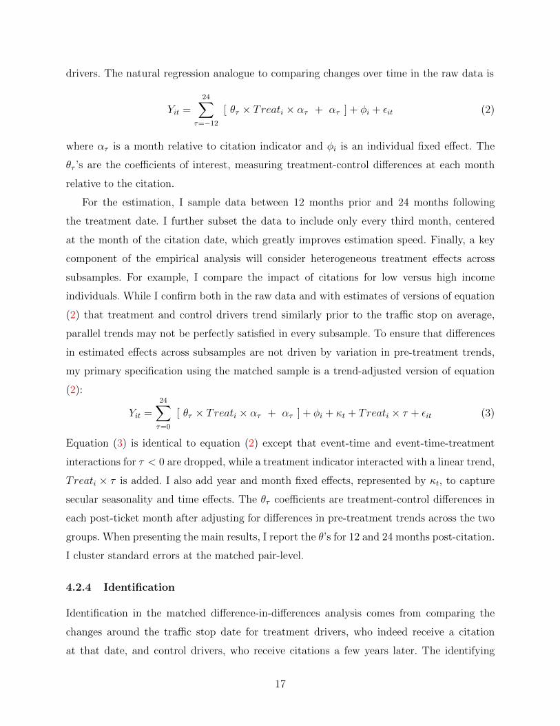
drivers. The natural regression analogue to comparing changes over time in the raw data is

Yit =24∑

τ=−12

[ θτ × Treati × ατ + ατ ] + φi + εit (2)

where ατ is a month relative to citation indicator and φi is an individual fixed effect. The

θτ ’s are the coefficients of interest, measuring treatment-control differences at each month

relative to the citation.

For the estimation, I sample data between 12 months prior and 24 months following

the treatment date. I further subset the data to include only every third month, centered

at the month of the citation date, which greatly improves estimation speed. Finally, a key

component of the empirical analysis will consider heterogeneous treatment effects across

subsamples. For example, I compare the impact of citations for low versus high income

individuals. While I confirm both in the raw data and with estimates of versions of equation

(2) that treatment and control drivers trend similarly prior to the traffic stop on average,

parallel trends may not be perfectly satisfied in every subsample. To ensure that differences

in estimated effects across subsamples are not driven by variation in pre-treatment trends,

my primary specification using the matched sample is a trend-adjusted version of equation

(2):

Yit =24∑τ=0

[ θτ × Treati × ατ + ατ ] + φi + κt + Treati × τ + εit (3)

Equation (3) is identical to equation (2) except that event-time and event-time-treatment

interactions for τ < 0 are dropped, while a treatment indicator interacted with a linear trend,

Treati × τ is added. I also add year and month fixed effects, represented by κt, to capture

secular seasonality and time effects. The θτ coefficients are treatment-control differences in

each post-ticket month after adjusting for differences in pre-treatment trends across the two

groups. When presenting the main results, I report the θ’s for 12 and 24 months post-citation.

I cluster standard errors at the matched pair-level.

4.2.4 Identification

Identification in the matched difference-in-differences analysis comes from comparing the

changes around the traffic stop date for treatment drivers, who indeed receive a citation

at that date, and control drivers, who receive citations a few years later. The identifying

17

assumption is that treatment drivers would have trended similarly to control drivers in the

absence of a traffic stop. As with most applications of difference-in-differences, there are two

primary threats to this assumption – different pre-treatment trends across treatment and

control groups and unobserved shocks correlated with both treatment status and treatment

timing. I verify that the two groups follow similar pre-treatment trends by examining the

raw data and estimating non-parametric event study-style specifications in the spirit of

equation (2) above. Further, to be conservative, I trend-adjust the regression estimates so

that coefficients are identified off deviations from pre-treatment trends as in equation (3).

By construction, treated and control drivers are approximately the same age at the time

of treatment. Hence, one can think of the identification strategy as leveraging differences

in the age at first (observed) citation, with treatment drivers first ticketed when a few

years younger than control drivers. Alternatively, one could think of the matching step as

identifying candidates for a traffic stop at a specific time and the analysis as comparing

candidates with stops that do and do not occur. In this framework, the empirical analysis

parallels studies that compare, for example, accepted and denied applicants around the time

of an application (e.g., Cellini et al. 2010, Mello 2018). Lastly, the empirical design is similar

to studies using individuals who receive treatment but outside the relevant time range as a

control group, such as Currie et al. (2018).

4.3 Estimating Impacts of License Suspensions

A potentially important mechanism through which traffic tickets may impact individuals

is through their impacts on driving privileges. Unpaid citations result in suspended driver

licenses, and a lack of a valid driver’s license may jeopardize an individual’s employment

arrangements. Additionally, the effects of license suspensions are of general interest, because

state and local governments use DL suspensions as punishment for an array of infractions.

For example, many states revoke driver licenses for individuals convicted of drug offenses.

While I cannot cleanly identify nonpayment of fines in the citations data, I estimate

the effect of suspensions levied for accruing too many driver license points. The majority of

citations carry three points and twelve points in twelve months results in a 30 day license

suspension. Hence, I estimate the impacts of license suspensions using an event study ap-

proach around the time of a fourth citation in one year. I also sample individuals receiving

18

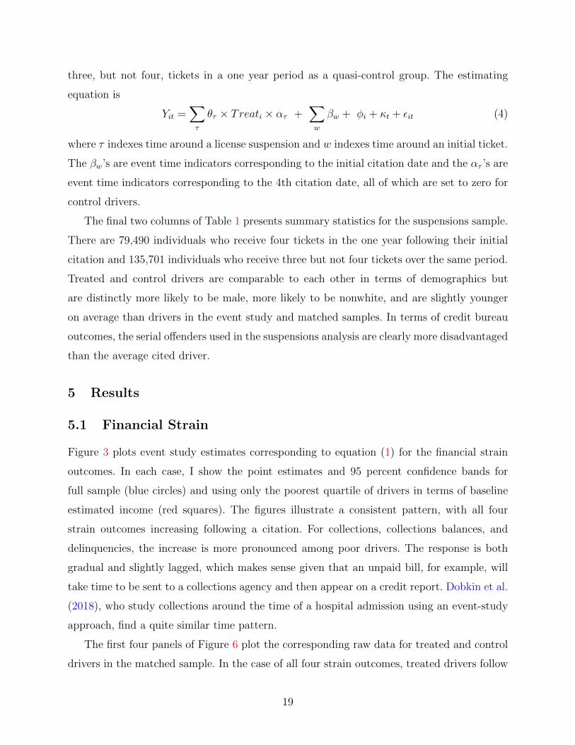
three, but not four, tickets in a one year period as a quasi-control group. The estimating

equation is

Yit =∑τ

θτ × Treati × ατ +∑w

βw + φi + κt + εit (4)

where τ indexes time around a license suspension and w indexes time around an initial ticket.

The βw’s are event time indicators corresponding to the initial citation date and the ατ ’s are

event time indicators corresponding to the 4th citation date, all of which are set to zero for

control drivers.

The final two columns of Table 1 presents summary statistics for the suspensions sample.

There are 79,490 individuals who receive four tickets in the one year following their initial

citation and 135,701 individuals who receive three but not four tickets over the same period.

Treated and control drivers are comparable to each other in terms of demographics but

are distinctly more likely to be male, more likely to be nonwhite, and are slightly younger

on average than drivers in the event study and matched samples. In terms of credit bureau

outcomes, the serial offenders used in the suspensions analysis are clearly more disadvantaged

than the average cited driver.

5 Results

5.1 Financial Strain

Figure 3 plots event study estimates corresponding to equation (1) for the financial strain

outcomes. In each case, I show the point estimates and 95 percent confidence bands for

full sample (blue circles) and using only the poorest quartile of drivers in terms of baseline

estimated income (red squares). The figures illustrate a consistent pattern, with all four

strain outcomes increasing following a citation. For collections, collections balances, and

delinquencies, the increase is more pronounced among poor drivers. The response is both

gradual and slightly lagged, which makes sense given that an unpaid bill, for example, will

take time to be sent to a collections agency and then appear on a credit report. Dobkin et al.

(2018), who study collections around the time of a hospital admission using an event-study

approach, find a quite similar time pattern.

The first four panels of Figure 6 plot the corresponding raw data for treated and control

drivers in the matched sample. In the case of all four strain outcomes, treated drivers follow

19

nearly identical trends to control drivers prior to the traffic stop date, suggesting a successful

matching procedure. However, trends diverge around the time of treatment, with treated

drivers exhibiting relative increases in collections, collections balances, derogatories, and

delinquencies following a traffic stop.

Table 2 plots the corresponding regression estimates. Each row corresponds to an out-

come and column 1 reports the baseline mean. Columns 2-3 report the 12 and 24 month

estimates from the event study approach, while columns 4-5 report the 12 and 24 month

estimates from the matched difference-in-differences approach. Event study estimates imply

that one year (two years) out from a traffic stop, individuals have about 0.09 (0.14) more

reported collections, 0.04 (0.05) more derogatory accounts, and 0.01 (0.02) more delinquen-

cies. Relative to the baseline means, the one (two) year effects are about three (five) percent

for collections, two (three) percent for derogatories, and two (three) percent for delinquen-

cies. In the fourth row, the outcome is an index that combines collections, derogatories, and

delinquencies, with the point estimate implying that traffic stops increase strain by about

2-3 percent of a standard deviation.18 Balances past due and balances in collections also

increase by about 2-5 percent. Estimates from the difference-in-differences approach are very

similar in most cases.

Table 3 reports estimates separately for the poorest and richest quartile of drivers.19 As

was apparent in Figure 3, the impact of traffic stops on collections is significantly larger for

poor than for rich drivers, with the disparity present across both research designs. Estimated

impacts on collections balances, for example, are 3-4 times larger for the poorest quartile of

drivers ($142) than for the richest ($38). The two year impact on collections balances for

poor drivers is over $200, larger than the size of the typical fine, in both specifications.

When considering heterogeneous effects on the account-based measures of financial strain,

we should keep in mind that richer drivers tend to have more accounts and higher balances

18The index is computed by standardizing each component, summing, and then standardiz-ing again. For the event study sample, I standardize relative to the base period. In the matcheddifference-in-differences approach, I standardize relative to the control group in the base period.

19The quartiles are determined using baseline estimated income in the matched sample. I use thesame thresholds when splitting the event study and license suspensions samples. Worth noting isthe fact that the rich quartile of drivers are not particularly well-off due to the apparent negativeselection into receiving a traffic ticket. Nearly 20% of the richest quartile of drivers has a subprimecredit score at baseline. Median estimated income among the richest quartile, about $53, 000, isbelow the 75th percentile of personal income in Florida.

20

(see Table 4), and therefore may have more space for growth in outcomes such as delinquen-

cies and adverse events. Still, I find larger impacts of traffic tickets on delinquencies for poor

than rich drivers. Event study estimates suggest similar effect sizes on derogatory events for

the richest and poorest quartiles, while the difference-in-difference estimates imply a larger

impact for poor drivers.

5.2 Payroll Employment

Figure 4 plots coefficients from event study estimates where the dependent variable is an

indicator for having positive payroll earnings in a given month. Recall that traffic tickets

may impact employment arrangements either through their impacts on financial distress,

which may reduce labor supply or job-finding rates, or through their impacts on driving

costs. Results for the full sample (blue circles) show a flat pre-event trend and a drop in

the likelihood of employment beginning in the first 2-3 months following a traffic stop and

persisting a full two years later. Poorer drivers appear to be trending slightly upward prior to

a traffic stop and experience a more dramatic drop following the date of a citation. The final

panel of Figure 6 plots the corresponding raw data from the matched sample, which reveals

a clear disparity between treatment and control drivers emerging only after the treatment

group’s traffic stop date.

Coefficients are reported in the first two rows of Table 4. For the full sample, regression

estimates imply a half a percentage point decline in the likelihood of positive earnings in

the payroll data, about a four percent decline relative to a baseline mean of twelve per-

cent. Difference-in-differences estimates are nearly identical. Table 5 compares effects for

the richest and poorest quartile of drivers and reveals that the impacts on employment are

significantly more pronounced among poor individuals. For the poorest quartile of drivers,

the one-year impact on employment is nearly a full percentage point (8 percent), while the

effect for rich drivers is about 0.3 percentage points (2.5 percent). The effect size disparities

between rich and poor drivers are even larger when considering the difference-in-differences

specification. Difference-in-differences in estimates of the employment (positive earnings)

effects for the richest quartile of drivers are not statistically different from zero.

Figure A-9 demonstrates that employment effects are driven both by an increase in the

likelihood that a currently employed individual transitions out of the payroll data and a

21

decrease in the probability that an individual transitions into the payroll data. Specifically, I

split the matched sample into individuals with and without payroll earnings as of 12 months

prior to the citation date and plot employment probability over time. The figure shows

that, relative to the control group, treated drivers in the payroll data at baseline become

more likely to transition out following a traffic stop. In the same vein, treated drivers not in

the payroll data at baseline become relatively less likely to transition into the payroll data

post-treatment.

Table A-4, which presents difference in difference estimates for payroll earnings, suggests

that traffic tickets have little impact on earnings for the average driver who remains in a

covered job. Figure A-7 plots event study coefficients where log monthly earnings is the

dependent variable. Consistent with the difference-in-difference estimates, there appears to

be little impact on earnings in the full sample. The event study estimates suggest a 1-2

percent decline in earnings for the poorest quartile of drivers, however. Neither the difference-

in-differences nor the event study estimates are precisely estimated.

5.3 Borrowing and Credit Usage

Event study estimates for the borrowing outcomes are plotted in Figure 5, while the raw

means for the matched sample are shown in Panels E-H of Figure 6. While we would expect a

surprise expense such as a traffic ticket to, if anything, increase financial strain, the predicted

impact of such a shock on borrowing is, ex ante, ambiguous. On one hand, an unplanned

expense may increase demand for credit. However, the impacts on financial duress discussed

above may reduce access to credit through their impacts on credit scores or borrowing limits.

While I estimate relatively small impacts of traffic stops on credit scores (about minus

two points as shown in Table A-3), other studies have found that collections may result in

reduced credit limits. Unfortunately, I do not observe borrowing limits in the credit report

data. Dobkin et al. (2018) estimate that hospital admissions increased collections balances

by $122 and, correspondingly, that credit limits fell by $500, despite also finding a small

effect on credit scores (-1.6).

Both the event study and matched difference-in-differences approaches illustrate a reduc-

tion in number of open revolving accounts following a traffic stop. The event study estimates

for revolving balances are noisy, but the raw means for matched treated and control drivers

22

suggest a relative decline in balances for treated drivers, although the response appears both

delayed in muted. For auto loans, the pattern of results is a bit strange, but if anything,

both the event study and matched difference-in-differences figures would suggest a decline

the likelihood of car ownership beginning 2-3 months following a citation. Both Panel D of

Figure 5 and Panel H of Figure 6 suggest a decline in the likelihood of having a mortgage. The

slightly lagged responses of revolving balances and durable consumption are consistent with

the view that access to credit is affected by the increases in financial strain and reductions

in employment documented above.

Regression estimates, presented in Table 4, show that traffic tickets induce about a 0.04

(1.5 percent) reduction in the number of open revolving accounts in the first year following

a traffic stop. Using the matched difference in differences approach, I find one and two

year effects on revolving balances of -$91 and -$218, with the two year estimate statistically

significant and implying about a three percent decline at the mean. Event study estimates are

smaller ($30-$50) and not statistically different from zero. Both strategies suggest statistically

significant declines in car and home ownership. While one should note that pre-event trends

in car ownership do not match perfectly for treated and matched control drivers, the trend-

adjusted matched difference-in-difference estimate is sizable. The two year estimate, -0.044,

represents about a thirteen percent reduction in the likelihood of having an open auto loan.

Both strategies suggest 1-2 percent reductions in the probability of home ownership.

Examination of heterogeneous effects by driver income, shown in Table 5, yields mixed

results. Estimated impacts of traffic tickets on revolving accounts are similar across the poor

and rich subsamples (-0.042 and -0.038 in the difference-in-differences specification), but

the similar point estimates imply quite different percent effects, -5 percent for poor drivers

and -0.6 percent for rich drivers, given the different baseline means. Both event study and

difference-in-differences approaches suggest a larger impact on auto loans for poor drivers,

but the rich-poor disparity is larger when considering the event study estimates.

5.4 Interpreting Magnitudes

The estimates for credit report outcomes suggest a consistent pattern of results, with traffic

tickets appearing to increase financial strain and reduce credit usage among cited drivers.

However, it is difficult to interpret the estimated magnitudes given that many of the credit

23

report measures are not what we would consider real outcomes. I use two approaches to aid

in the interpretation of the results, detailed below.

5.4.1 Benchmarking to Other Studies

The most similar study to mine is Dobkin et al. (2018), who examine the impact of hospital

admissions on credit report outcomes using an event study approach. Table 6 allows for

a comparison of effect sizes between my paper and Dobkin et al. (2018) (referred to as

DFKN in the table). Panel A highlights that the hospital admissions sample is older and

more advantaged than the cited driver sample. However, the financial shock accompanying

a hospital admission is also more severe. For the nonelderly insured population, the authors

estimate that an average hospital admission increases out-of-pocket medical expenditures by

about $3,300.

As shown in Panel B, estimated 12 month effects of traffic tickets and hospital admissions

on collections (0.075, 0.11) and collections balances ($94, $122) are quantitatively similar.

Given that the average individual in the hospital sample has fewer collections, however, the

percent effects are larger in Dobkin et al. (2018). As shown in Panel B, hospital admissions

are associated with a slightly larger decline in revolving balances, -$293 (-2.5 percent), than

are traffic tickets, -$91 (-1.3 percent). On net, the estimated impacts on financial wellbeing

appear relatively similar across the two contexts, which perhaps makes sense when consid-

ering the larger shock but more advantaged sample in the Dobkin et al. (2018) study.

For context, I also present estimated effects from two other studies in Table 6. Note that

both Herbst (2018) and Dobbie et al. (2017) study positive shocks, and hence the effects are

opposite-signed. Herbst (2018) finds similar effects to mine of income-driven student loan

repayment plans on the number of revolving accounts but larger effects on balances. Un-

surprisingly, Dobbie et al. (2017) find significantly larger impacts of Chapter 13 bankruptcy

protection on financial health outcomes.

5.4.2 Benchmarking to Earnings Changes

An alternative method for benchmarking magnitudes is to ask what change in income would

predict the observed increases in financial strain. To approximate this thought experiment, I

take a cross-section of individuals from the matched sample as of three months prior to the

traffic stop date with positive payroll earnings. I then fit annualized payroll earnings to a

24

quartic in each financial strain measure.20 Using the estimated quartic coefficients combined

with the treatment effect estimate, I compute the income change predicted by the estimated

financial stain effects. Specifically, for strain outcome z, I compute

∆̂(z) =∂y

∂z

(β̂, z̄)× θ̂z.

In words, ∆̂ is the derivative of income with respect to z, a function of the quartic coefficients

β̂ and evaluated at the sample mean of z, scaled by the estimated treatment effect of citations

on z from Table 2. In additional to the individual account measures, I compute the income

metric for the strain index, which can we interpret as the income change implied by the joint

changes in the strain outcomes.

The results are presented in Table 7. Columns 1 and 2 show income losses implying

the difference-in-differences strain coefficients as of 12 and 24 months post citation for the

full sample, while columns 3-6 repeat the analysis for the poorest and richest quartile of

the sample corresponding to the main result tables. In each case, I evaluate at the relevant

baseline mean shown in Table 2 and Table 3. Below the computed dollar values, I show the

implied percentage change in income, evaluated at the relevant sample mean, in brackets.

Row 1 indicates that the sample-wide, one-year impact on collections, 0.075, is about

what would be predicted by a $360 reduction in annual outcome. For poor drivers, the

income-equivalent effect is much larger. The 12 and 24 month increases in collections are

associated with predicted income changes of $663 and $951, respectively. In other words,

a poor individuals’ long-run post-citation increase in collections is observationally similar

to about a 5.5 percent income loss. The estimated treatment effects on derogatories and

delinquencies are notably smaller, and therefore the income-equivalent effects are smaller as

well. The income loss predicting the observed increase in the strain index similar to that

predicting the collections effect alone.

It is also useful to benchmark the treatment effects against the estimated impacts sepa-

rations from payroll-covered jobs, which are presented in Appendix C. The effect of a traffic

ticket on collections (0.075) is about two-thirds as large as the effect of a job separation

(0.114), while the ticketing effect on revolving balances is (-$95) is about one third as large

20A flexible functional form is important for fitting the data well. The observed relationshipbetween, for example, number of collections, and earnings is highly nonlinear, with a steep gradientat low values of collections and a much flatter gradient at high values.

25

as the separation effect (-$280). Job separations increase delinquencies by 0.2, or about

twice as much as traffic fines. The estimated impacts of job separations and traffic tickets

on derogatories and collections balances are similar, while the citation effect on number of

credit cards is about 40 percent larger than the separation effect.

5.5 Heterogeneity

As discussed above, the impacts of traffic tickets on financial strain and employment differed

meaningfully for high- and low-income drivers. In this section, I consider heterogeneity along

other dimensions. To be parsimonious, I first consider only impacts on the financial strain

index and employment using the matched difference-in-differences framework.

Figure 7 plots one year difference-in-differences estimates for the strain index across sub-

sets of drivers. Impacts are larger for younger (under 35) than for older (over 35) drivers and

appear similar for women and men. Treatment effect estimates are similar for subprime and

prime individuals, but are more pronounced for individuals with low credit usage, measured

either as having a below median revolving balance or having any durable account at base-

line. The most striking cut of the data is along the dimension of baseline collections. Traffic

tickets have no effect on strain for drivers with a collections balance below $150 at baseline,

suggesting that the entire effect is driven by individuals who already have unpaid bills.

Figure 8 is identical to Figure 7 except that the dependent variable is employment.

The pattern of heterogeneity is similar – subsamples with a large strain effects also tend

to have larger employment effects and vice versa. Treatment effects on employment are

larger for younger individuals and especially pronounced for young women, and are larger

for individuals with higher collections, lower credit scores, and less borrowing at baseline.

Motivated by the striking difference in strain impacts across individuals with high and

low initial collections, I present one year difference-in-differences estimates by baseline credit

score and collections for all outcomes in Table 8. Note that below the standard errors, I

report the relevant baseline control mean in brackets. As mentioned previously, one caveat

with interpreting differences in effects on borrowing-related outcomes across subsamples is

that credit usage may also differ across samples. Subprime individuals maintain about one

quarter as many revolving accounts, for example, and individuals who do not maintain open

accounts cannot experience increases in delinquencies or decreases in balances.

26

As shown in columns 2-3, impacts on collections and employment are about two times as

large for subprime than for prime individuals. The disparate collections effect makes sense

– credit is more readily available for prime individuals, and such individuals may be able to

cover the unexpected nuisance fine through borrowing.

The effect size gaps are even larger when comparing individuals with high and low base-

line collections in columns 4-5. Point estimates for collections and adverse financial events

are, in fact, negative for individuals with little to no balance under collection at baseline. In-

dividuals with above median baseline collections balances experience a four percent increase

in collections, a six percent increase in collections balances, and a four percent increase in

derogatory accounts in the one year following a traffic stop. Reductions in revolving accounts

and revolving balances are also driven entirely by individuals with unpaid bills at baseline.

The effect of a traffic ticket on payroll employment is about two and a half times larger for

the high collections sample.

Overall, there is a clear pattern to the heterogeneity of the results. For individuals ex-

hibiting financial stability at baseline, e.g. those without unpaid bills and those with high

credit scores, traffic citations have minimal impacts. Drivers showing signs of instability,

such as high collections balance, low credit scores, and low borrowing, experience significant

increases in measures of financial strain and the largest drops in employment. This set of

results suggests the presence of a poverty trap where small shocks have deleterious effects

on already distressed individuals but are negligible for the non-distressed population.

The notion of the poverty or financial distress strap is shown empirically in Figure 9.

The figure shows one year (blue circles) and two year (red squares) difference-in-differences

estimates of the impact of a traffic stop on the financial strain index, estimated separately

by quantiles of strain at baseline. The one year treatment effects are clearly increasing in

baseline strain. Through much of the distribution, the gradient in the two year effects is even

stronger. In other words, the effect of a small shock is larger for more distressed individuals

and, further, effect sizes increase more over time for such individuals.

5.6 Mechanisms

As detailed in the discussion of the institutional background, a traffic citation represents a

potentially multi-faceted treatment, with the exact treatment faced by any given individual

27

depending on post-citation decisions such as whether the individual chooses not to pay or

opts to contest the ticket. While it is useful to note that the Florida Clerk’s office’s records

indicate that over 90% of citations are paid on time, the data from the Florida Clerks include

some information on the court disposition associated with each citation that is potentially

useful for disentangling the relative important of the aspects of traffic fines beyond the pure

expense shock in explaining the estimated effects. 21

Specifically, I examine treatment effects for individuals whose dispositions indicate pay-

ment and those whose dispositions indicate a traffic school election. Individuals making

on-time payment may opt to participate in traffic school, which consists of four hours of in-

struction and costs $25, but suppresses the points associated with the citation from accruing

on the driver’s record. Because she makes an on-time payment and faces no increase in license

points, a driver opting for traffic school almost surely will not suffer a license suspension or

an increase in car insurance premiums.22

Comparing payers and school-attendees to the sample as a whole and to each other

should help isolate the impacts of various components of the treatment. The typical payer

will not incur a license suspension, but those with significant driving histories or making late

payments may. Payers will incur increased license points possibly leading to increased auto

insurance costs. Traffic schools attenders will not bear any burden of license suspensions or

increased license points. However, a traffic school election signals a savviness of institutions,

an ability to come up with an extra $25, and the flexibility to participate in four hours of

instruction. As shown in the footer of Table 9, school participants are older, richer, and have

higher credit scores. While I cannot account for unobservable differences between the two

groups of drivers, I do present estimates using the reweighting scheme from DiNardo et al.

(1996) to account for observable differences across the subsamples at baseline. Specifically,

I group the data into cells according the baseline age, income, and credit score bands used

in the matching step. I then reweight the cells in the payer and school subsamples to match

the distribution in the full sample.

21There are important caveats to consider regarding the court dispositions data. Traffic citationsare resolved through the ticketing county’s court system. The individual county clerks then sharedisposition information with the Florida Clerk of Courts. However, many of the disposition-relatedfields are not required to be shared with the state clerk. Futher, information on dispositions reflectcurrent status. A disposition indicating payment may not reflect on-time payment, for example.

22Moreover, due to concerns over the quality of the dispositions data raised earlier, traffic schoolattendees are the only subsample who are guaranteed to have made on-time payment.

28

Table 9 shows the one-year difference-in-differences estimates for the financial strain index

and employment by disposition. Columns 2-3 indicate that the impact of a citation on strain

is nearly two times larger for payers than for individuals opting for traffic school. Similarly,

employment effects are about 50 percent larger for payers, with the point estimate not

statistically significant in the traffic school sample. While neither difference is statistically

significant, the pattern of results is consistent with the hypothesis that the potential costs of

tickets beyond the pure financial shock, particularly those associated with increased driver

license points, are an important driver of the results.23

However, columns 4-5 reveal that the treatment effect disparities are much smaller after

reweighting the data to account for observable differences between the two samples. While

the point estimates still suggest that those attending traffic school experience slightly smaller

increases in financial strain, the narrowing of the treatment effect disparities suggests that

differences in the type of individuals opting for traffic school are quite important in explaining

the treatment effect disparities. On net, the evidence provides some support for the view

that license suspensions and increased insurance costs are relevant for explaining the impact

of tickets but also highlights that individuals making on-time payment still experience a

worsening in financial standing. The small effects for school attendees using the unweighted

data supports the view that the type of individual choosing traffic school is less susceptible

to the harm caused by a citation.

5.7 Effects of License Suspensions

I supplement the comparison of effects across disposition types with a direct analysis of

license suspensions due to the accrual of driver license points using the empirical approach

described in section 4.3. Figure 10 plots event study coefficients around the time of an

individual’s fourth citation in twelve months, with proxies for the timing of a 30-day points-

based license suspension. Recall that the regressions also include indicators for months since

initial citation (and use individuals accruing three but not four tickets in twelve months to

help in the estimation of these coefficients), so the estimates should be interpreted as additive

23Another piece of evidence consistent with this view is presented in Figure A-12 in the appendix,which plots estimated impacts of citations by quantiles of the imputed fine amount and showsminimal treatment effect gradients with respect to fine size. If effects are due only to financialshocks, we might expect larger impacts associated with larger fines.

29

to the effects of an initial traffic stop.

Panels A and B document sharp increases in collections following a license suspension.

Quantitatively, the impact appears more pronounced than for the average traffic stop, and

strikingly, the increase in collections is nearly as large for the typical driver as for the poor-

est individuals.24 Panel C documents a fall in borrowing, measured with revolving balances,

coinciding with the timing of a license suspension. Finally, Panel D illustrates an immediate

and sustained drop in the likelihood of having positive payroll earnings following the revo-

cation of driving privileges. The short-run fall in employment appears more pronounced for

the poorest quartile of drivers. Figure A-14 plots event study coefficients for other outcomes.

I present the coefficient estimates in Table 10. One year out from a license suspension,

individuals have about 0.15 (4 percent) more collections and $140 (5 percent) higher col-

lections balances. Both effects are larger than the one-year event study estimates focused

on an initial citation. Incidences of adverse financial events increase by about 4 percent. I

also find evidence of a slight increase in bankruptcy, measured by the presence of any public

records bankruptcy filing in the past 24 months on a credit report, following a suspension.

Revolving balances and employment probability are about 2.5 percent and 3 percent lower

one year out from a suspension. As shown in Panel B, estimated effects are slightly larger

for the poorest subset of drivers. Recall from Table 1 that the license suspension sample is

more disadvantaged, and therefore the poor driver group is more representative of the sample

as a whole than in the analysis of initial citations. On average, one year impacts are 10-25

percent larger for poorer drivers. Poor drivers experience larger drops in employment (about

5 percent), but no increase in bankruptcy filings, likely due to the fact that bankruptcy is

quite rare among individuals without much borrowing.

The analysis of license suspensions is not only independently interesting, but also can

provide insights about the mechanisms underlying the main results. Some of the estimated

effect of citations alone is almost certainly due to suspensions imposed on individuals electing

non-payment or those with poor driving records at baseline, both of which are difficult

to observe directly in the data. The fact that the effects of suspensions on wellbeing are

substantial lends credence to this view. On the other hand, the suspension effects are not

24Note that I use a baseline estimated income of $21,000 as the threshold for the poorest subsetin the suspensions analysis for comparability between citation effects and suspensions effects amongpoor drivers. $21,000 is the 37th percentile of baseline estimated income in the suspensions sample.

30

enormous relative to the main estimates, implying that the treatment effects of citations

cannot be due only to ensuing license suspension effects. The observation that citations

increase distress even among individuals who participate in traffic school, discussed above,

also supports this claim.

6 Estimating Welfare Effects

6.1 Framework

Thus far, we have considered an array of evidence illustrating declines in wellbeing in the

two years following a traffic stop. To quantify welfare losses, I adapt a common approach

for valuing policies (e.g. Finkelstein et al. 2015, Deshpande 2016) to the dynamic nature of

the treatment effects. The approach approximates the following thought experiment – at the

time of the traffic stop, how much would an individual be willing to pay to avoid the ensuing

utility loss? Specifically, assume individuals have utility over consumption u(c) and discount

the future at rate β. Let D be an indicator for whether an individual receives a traffic ticket

at t = 0. The parameter of interest is V from the following equation:

u(c0 − V ) +T∑t=1

βtu(ct|D = 0) = u(c0) +T∑t=1

βtu(ct|D = 1). (5)

The left hand side is the utility value of the consumption path for an unticketed driver

except that the individual pays V at time zero. The right hand side is the consumption

path for a ticketed driver. V is the foregone consumption at t = 0 that makes an individual

indifferent between the ticketed and unticketed consumption streams, which we can interpret

as willingness to pay to avoid the negative downstream consequences of a traffic ticket.

Solving equation (5) requires a function form assumption on u(·), as well as estimates of

the two consumption streams. A common form for u(·) is a constant relative risk aversion

(CRRA) utility function,

u(c) =c1−γ

1− γI take γ = 1, implying a logarithmic utility function, the mean estimate in Chetty (2006b), as

a benchmark. Note that, in this framework, increasing the curvature in the utility function

will typically reduce estimates of V by increasing the pain associated with the one-time

31

payment at low levels of c.

For simplicity, I consider one- and two-year effects and assume individual’s discount the

future at rate 0.96. To estimate the consumption paths, I take a proxy measure y and use

means over (event) time as the untreated consumption path. I then add the month specific

treatment effects from estimates of (3) to the means to obtain the treated consumption

stream:

[ct|D0 = 0] = µyt , [ct|D0 = 1] = µyt + θ̂t.

where µyt is the mean of y for the control group at time t.

6.2 Estimating Consumption

Even in credit report data, consumption is not observed. The most straightforward ap-

proach to estimating consumption is to assume no savings and proxy consumption with

income. While income is not observed directly for individuals without payroll earnings, I can

approximate income changes using either the credit bureau’s estimated income measure or

using the employment treatment effects combined with an assumption about the earnings

loss associated with employment transitions. For the average driver, difference-in-differences

estimates imply one- and two-year reductions in estimated income of $189 and $385 (see Ta-

ble A-3). At the mean estimated income of $33,000, and assuming log utility and β = 0.96,

these effects imply V = $534.

Alternatively, using the estimated employment impacts does not rely on a measure of

unknown origin, but requires two important assumptions. First, one needs an assumption

about how the employment estimates should be scaled. Difference in differences estimates

suggest declines in employment by between one half and three quarters of a percentage point,

but rely on an employment measure with low coverage. Scaling by the coverage and assuming

a population-wide employment rate of about 90 percent, the estimates imply one and two

year employment declines of 2.7 and 4.5 percentage points. Second, one needs an assumption

on earnings losses occurring from employment transitions. A comparison of payroll earnings

with ACS data in the matched sample implies payroll covered jobs pay about $8,000 more

annually. Hence, a back-of-the envelope calculation suggests one and two year income losses

of $216 ($8, 000× .027) and $360, yielding a very similar estimate of V .

These welfare calculations ought to be considered conservative. I consider two year im-

32

pacts because that is the time horizon that can be reliably studied in the data. In nearly all

cases, treatment effects persist for the full two years. To the extent that the effects persist or

grow in the long-run, an estimate of V based on a two-year window is understated. Moreover,

the impacts on outcomes such as collections and adverse financial events may have long-run

impacts on access to credit, diminishing an individual’s ability to smooth consumption in

the future and resulting in additional utility losses. Finally, the computation of V does not

consider welfare effects associated with the reductions in durable consumption.

6.3 Discussion

While simplistic, the above welfare calculation is useful for considering the policy implications

of my findings more generally. Before discussing the relevance of the results for policing,

however, it is important to note the argument of Atkinson & Stiglitz (1976) that welfare

losses induced through commodity taxation, in this case the taxation of traffic infractions,

ought to be remedied with redistribution through the income tax system. Moreover, the

finding that many low-income households are not insured against expense shocks suggests

that social programs offering insurance against expenditure or income risk may yield large

benefits.

To consider the implications of my findings for criminal justice policy, note that existing

evidence and standard economic theory would suggest that local governments have two goals

when issuing traffic tickets — promoting safety and raising revenue. For example, DeAngelo

& Hansen (2014), Makowsky & Stratmann (2011), and Luca (2015) show that increases in

traffic citations reduce car accidents. Baicker & Jacobson (2007), Makowsky & Stratmann

(2009), and Garrett & Wagner (2009) find evidence of a revenue-raising motive in policing

decisions. Standard models for analyzing criminal justice policy typically build on Becker

(1968), and I present a formal Becker-style model in Appendix B.

The intuition of the model is that an increase in the traffic ticketing rate deters dangerous

behavior by increasing the probability that an individual is audited and sanctioned, but is

costly in terms of policing effort and reduces the welfare of offenders. Increased ticketing also

raises government revenue. Optimal policing will set marginal benefits equal to marginal

33

costs:

−h′(p)︸ ︷︷ ︸marginal safety benefit

+ r︸︷︷︸marginal revenue benefit

= c′(p)︸︷︷︸marginal cost of policing

− V ′(p)︸ ︷︷ ︸marginal welfare loss

To the extent that a citation represents a lump-sum transfer from an individual to the

government, there are no efficiency implications. An optimizing government should then

trade off the marginal labor costs and marginal deterrence benefits when deciding the optimal

policing intensity.

However, welfare losses associated with citations exceeding the size of the transfer can

be considered deadweight loss and ought to be weighed against the deterrence benefits when

optimizing ticketing intensity. The welfare metric introduced above, which is an individual’s

willingness to pay to avoid future utility losses, embodies the notion of deadweight loss

well.25 I find that the typical ticket, which imposes a fine of about $175, induces welfare

losses slightly larger than $500, implying that the safety benefit associated with a marginal

citation must exceed $300 for its issuance to be optimal. More generally, if governments

set optimal enforcement without taking into account the compounding welfare effects of

fines, they will tend to over-police. Quantifying deterrence benefits is beyond the scope of

this paper, but one could speculate that citations issued for minor offenses such as broken

taillights or marginal citations at already high rates of ticketing are unlikely to provide much

return in terms of safety.

The heterogeneous welfare consequences of fines across driver-income levels also highlight

the potential inefficiency of the flat traffic fine schedule. Appendix B considers in detail the

implications of an income-based fine schedule. In particular, I present a stylized environment

with two types of individuals, low-income (yL) and high-income (yH) and consider the effects

of moving from a one-size-fits-all fine f0 to a scheme that charges high-income drivers f0 +

∆ and low-income drivers f0 − ∆, where ∆ is positive, small, and satisfies an additional

simplifying assumption detailed in the appendix. The welfare effects of such a policy change

25Note that, as shown in Appendix B, for the class of marginal criminals, the welfare cost asso-ciated with writing one more citation is 1

1−p [u(y − f) − u(y)], which for small p is approximatelythe utility cost associated with being sanctioned, i.e. the quantity V estimated above.

34

are proportional to the difference in the marginal utilities for poor and rich drivers:

∆×[∂u

∂c(yL − f0)− ∂u

∂c(yH − f0)

]︸ ︷︷ ︸

difference in marginal utilities

× p[1−G(x∗)]︸ ︷︷ ︸number of tickets

(6)

which is positive when u(·) is concave. The empirical estimates suggest that the difference

in marginal utilities is potentially large. Under various assumptions about the compounding

utility consequences of fines for poor drivers and values of γ, and taking into account that

about two million citations are issued in Florida annually, the welfare gains to setting ∆ = $10

are between $6 and $21 million per year. Using the result in section 6.3, the total utility cost

of traffic tickets is about $2 billion, implying that the simple $10 fine perturbation could

erode the welfare costs of enforcement by as much as one percent.

7 Conclusion

Motivated both by the observation that the incidence of policing falls largely on disadvan-

taged communities and by a growing body of evidence suggesting that many low-income

individuals may be unable to cope with unexpected expenses, this paper studies the effect of

fines for traffic violations on financial wellbeing. To estimate causal effects, I link adminis-

trative traffic citation records to high frequency credit report and payroll data and leverage

variation in the timing of traffic stops for identification.

The empirical analysis reveals that following the receipt of a traffic fine, individuals fare

worse than would otherwise be predicted on a host of credit report outcomes. Citations

increase unpaid bills, delinquencies, and adverse financial events, with the increases most

pronounced for the poorest quartile of drivers. For the average driver, the short-run increases

in measures of financial strain are about what would be predicted by a $285 income loss. For

the poorest drivers, the two-year increases in financial distress are observationally similar

to an $800-900, or about 5 percent, income reduction. I also find evidence of a decline in

borrowing, measured by revolving accounts and balances, as well as the presence of home

and auto loans on credit reports, following a traffic stop

Traffic tickets reduce the likelihood that an individual appears as having any earnings in

payroll data covering large employers by about 0.5 percentage points, or almost 5 percent

relative to the mean. The employment effects are, again, most pronounced among the poor-

35

est drivers. Poor drivers experience an 8 percent drop in the probability of having payroll

earnings in the one year following a traffic stop.

The findings offer several important takeaways. First, consistent with a growing literature

documenting widespread financial fragility among U.S. households, the results imply that

many individuals are not insured against even small financial shocks. When faced with a $175

traffic fine, individuals accrue collections and delinquencies on their credit reports, suggesting

an inability to cover the unexpected expense. Second, individuals exhibiting minimal distress

at baseline are largely unaffected by nuisance fines, while those already facing several unpaid

bills experience the most significant declines in financial wellbeing. This pattern of results is

consistent with a poverty trap, whereby already distressed individuals are derailed by a new

expense. Third, both the pure financial shock component of a traffic citation and the ensuing

increases in driving costs, either through increases in insurance premiums or the revocation of

driving privileges, appear to be important mechanisms. And fourth, a conservative estimate

of the welfare loss associated with the average traffic ticket is more than two times the size of

the revenue raised, suggesting that policies to reduce citations with low public safety benefits

could be welfare enhancing.

36

References

Adams, R. (2015). In Florida, Failure to Pay Fees can Result in Suspended License — andthen More Fees. Miami Herald, 1–13.

Agarwal, S., Liu, C., & Souleles, N. (2007). The Reaction of Consumer Spending and Debtto Tax Rebates—Evidence from Consumer Credit Data. Journal of Political Economy,115 (6), 986–1019.

Aneja, A. & Avenancio-Leon, C. (2017). Credit-Driven Crime Cycles: The Connection Be-tween Incarceration and Access to Credit. Working Paper, 1–70.

Ang, D. (2018). The Effects of Police Violence on Inner-City Students. Working Paper,1–72.

Angrist, J. & Pischke, J.-S. (2009). Mostly Harmless Econometrics. Princeton UniversityPress.

Atkinson, A. & Stiglitz, J. (1976). The Design of Tax Structure: Direct Versus IndirectTaxation. Journal of Public Economics, 6 (1-2), 55–75.

Atkinson, A. & Stiglitz, J. (2015). Lectures on Public Economics. Princeton UniversityPress.

Atkinson, T. (2016). A Fine Scheme: How Municipal Fines Become Crushing Debt in theShadow of the New Debtors Prison. Harvard Civil-Rights Civil-Liberties Law Review,189 (51), 189–238.

Avery, R., Calem, P., Canner, G., & Bostic, R. (2003). An Overview of Consumer Data andCredit Reporting. Federal Reserve Bulletin, 47 (89), 47–73.

Baicker, K. & Jacobson, M. (2007). Finders keepers: Forfeiture laws, policing incentives, andlocal budgets. Journal of Public Economics, 91 (11-12), 2113–2136.

Baily, M. (1978). Some Aspects of Optimal Unemployment Insurance. Journal of PublicEconomics, 10, 379–401.

Balko, R. (2018). The Ongoing Criminalization of Poverty. The Washington Post, 1–3.

Banerjee, A. & Duflo, E. (2011). Poor Economics. Public Affairs.

Barrett, C., Carter, M., & Chavas, J.-P. (Eds.). (2019). The Economics of Poverty Traps.University of Chicago Press.

Bartik, A. & Nelson, S. (2017). Credit Reports as Resumes: The Incidence of Pre-Employment Credit Screening. Working Paper, 1–54.

Baugh, B., Itzhak, B.-D., & Park, H. (2014). Disentangling Financial Constraints, Pre-cautionary Savings, and Mypoia: Household Behavior Surrounding Federal Tax Returns.NBER Working Paper, 1–42.

37

Becker, G. (1968). Crime and Punishment: An Economic Approach. Journal of PoliticalEconomy, 76 (2), 169–217.

Beshears, J., Choi, J., Laibson, D., & Madrian, B. (2018). Behavioral Household Finance.Technical Report 24854.

Board of Governors of the Federal Reserve System (2018). Report on the Economic Well-Being of U.S. Households in 2017. Technical report.

Borusyak, K. & Jaravel, X. (2017). Revisiting Event Study Designs. Working Paper, 1–25.

Brevoort, K., Grimm, P., & Kambara, M. (2015). Data Point: Credit Invisibles. ConsumerFinancial Protection Bureau, 1–37.

Brown, C. & Medoff, J. (1989). The Employer Size-Wage Effect. Journal of Political Econ-omy, 97 (5), 1027–1059.

Burlando, A. & Motta, A. (2016). Legalize, Tax, and Deter: Optimal Enforcement Policiesfor Corruptible Officials. Journal of Development Economics, 118, 207–215.

Card, D., Chetty, R., & Weber, A. (2007). Cash-on-hand and Competing Models of Intertem-poral Behavior: New Evidence from the Labor Market. Quarterly Journal of Economics,122 (4), 1511–1560.

Cardiff-Hicks, B., Lafontaine, F., & Shaw, K. (2015). Do Large Modern Retailers Pay Pre-mium Wages? ILR Review, 68 (3), 633–665.

Carnegie, J. (2007). Driver’s License Suspensions Impacts and Fairness Study. NJ DOTReport, 1–83.

Carroll, C. (1992). The Buffer-Stock Theory of Saving: Some Macroeconomic Evidence.Brookings Papers on Economic Activity, 2, 61–156.

Carroll, C. (1997). Buffer-Stock Saving and the Life Cycle/Permanent Income Hypothesis.Quarterly Journal of Economics, 112 (1), 1–55.

Cellini, S., Ferreira, F., & Rothstein, J. (2010). The Value of School Facility Investments: Ev-idence from a Dynamic Regression Discontinuity Design. Quarterly Journal of Economics,125 (1), 215–261.

Chalfin, A. & McCrary, J. (2017). Criminal Deterrence: A Review of the Literature. Journalof Economic Literature, 55 (1), 5–48.

Chetty, R. (2006a). A general formula for the optimal level of social insurance. Journal ofPublic Economics, 90 (10-11), 1879–1901.

Chetty, R. (2006b). A New Method of Estimating Risk Aversion. American EconomicReview, 96 (5), 1821–1834.

38

Chetty, R. & Szeidl, A. (2007). Consumption Commitments and Risk Preferences. QuarterlyJournal of Economics, 122 (2), 831–877.

Corbae, D. & Glover, A. (2018). Employer Credit Checks: Poverty Traps Versus MatchingEfficiency. NBER Working Paper, 1–63.

Corman, H. & Mocan, N. (2005). Carrots, Sticks, and Broken Windows. The Journal ofLaw and Economics, 48 (1), 235–266.

Council of Economic Advisors (2015). Fines, Fees, and Bail. CEA Issue Brief, 1–12.

Cullen, J., Friedberg, L., & Wolfram, C. (2005). Do Households Smooth Small ConsumptionShocks? Evidence from Anticipated and Unanticipated Variation in Home Energy Costs.Center for the Study of Energy Markets Working Paper, 1–33.

Currie, J., Mueller-Smith, M., & Rossin-Slater, M. (2018). Violent While in Utero? TheImpact of Assaults During Pregnancy on Birth Outcomes. NBER Working Paper, 1–56.

DeAngelo, G. & Hansen, B. (2014). Life and Death in the Fast Lane: Police Enforcementand Traffic Fatalities. 6 (2), 231–257.

Deaton, A. (1991). Saving and Liquidity Constraints. Econometrica, 59 (5), 1221–1248.

Department of Justice Civil Rights Division (2015). The Ferguson Report: Department ofJustice Investigation of the Ferguson Police Department. The New Press.

Deshpande, M. (2016). Does Welfare Inhibit Success? The Long-Term Effects of RemovingLow-Income Youth from the Disability Rolls. American Economic Review, 106 (11), 3300–3330.

Desmond, M. (2016). Evicted. Crown Books.

DiNardo, J., Fortin, N., & Lemieux, T. (1996). Labor Market Institutions and the Distribu-tion of Wages, 1973-1992: A Semiparametric Approach. Econometrica, 64 (5), 1001–1044.

Dobbie, W., Goldsmith-Pinkham, P., Mahoney, N., & Song, J. (2018). Bad Credit, NoProblem? Credit and Labor Market Consequences of Bad Credit Reports. Working Paper,1–75.

Dobbie, W., Goldsmith-Pinkham, P., & Yang, C. (2017). Consumer Bankruptcy and Finan-cial Health. Review of Economics and Statistics, 99 (5), 853–869.

Dobbie, W. & Song, J. (2015). Debt Relief and Debtor Outcomes: Measuring the Effects ofConsumer Bankruptcy Protection. American Economic Review, 105 (3), 1272–1311.

Dobkin, C., Finkelstein, A., Kluender, R., & Notowidigdo, M. J. (2018). The EconomicConsequences of Hospital Admissions. American Economic Review, 108 (2), 308–352.

Enamorado, T., Fifield, B., & Imai, K. (2017). Using a Probabilistic Model to Assist Mergingof Large-scale Administrative Records. Working Paper, 1–54.

39

Federal Reserve Bank of New York (2018). Quarterly Report on Household Debt and Credit,1–33.

Fernald, L. C. H. & Gunnar, M. R. (2009). Poverty-alleviation program participation andsalivary cortisol in very low-income children. Social Science & Medicine, 68 (12), 2180–2189.

Finkelstein, A., Hendren, N., & Luttmer, E. (2015). The Value of Medicaid: InterpretingResults from the Oregon Health Insurance Experiment. NBER Working Paper, 1–63.

Finkelstein, A., Taubman, S., Wright, B., Bernstein, M., Gruber, J., Newhouse, J. P., Allen,H., Baicker, K., & Oregon Health Study Group (2012). The Oregon Health InsuranceExperiment: Evidence from the First Year. The Quarterly Journal of Economics, 127 (3),1057–1106.

Fonseca, J., Strair, K., & Zafar, B. (2017). Access to Credit and Financial Health: Evaluatingthe Impact of Debt Collection. Woring Paper, 1–45.

Gallagher, J. & Hartley, D. (2017). Household Finance after a Natural Disaster: The Caseof Hurricane Katrina. American Economic Journal: Economic Policy, 9 (3), 199–228.

Ganong, P. & Noel, P. (2017a). Consumer Spending During Unemployment: Positive andNormative Implications. Working Paper, 1–81.

Ganong, P. & Noel, P. (2017b). The Effect of Debt on Default and Consumption: Evidencefrom Housing Policy in the Great Recession. Working Paper, 1–97.

Garrett, T. & Wagner, G. (2006). Are Traffic Tickets Countercyclical? Federal Reserve Bankof St. Louis Working Paper Series, 1–22.

Garrett, T. & Wagner, G. (2009). Red Ink in the Rearview Mirror: Local Fiscal Conditionsand the Issuance of Traffic Tickets. The Journal of Law and Economics, 52 (1), 71–90.

Gehrsitz, M. (2017). Speeding, Punishment, and Recidivism: Evidence from a RegressionDiscontinuity Design. Journal of Law and Economics, 60, 497–528.

Goldstein, R., Sances, M., & You, H. Y. (2018). Exploitative Revenues, Law Enforcement,and the Quality of Government Service. Urban Affairs Review, 1–27.

Goncalves, F. & Mello, S. (2017). Does the Punishment Fit the Crime? Speeding Fines andRecidivism. Working Paper, 1–49.

Goncalves, F. & Mello, S. (2018). A Few Bad Apples? Racial Bias in Policing. IndustrialRelations Section Working Paper, 1–88.

Gorzelany, J. (2012). Got A Ticket? Here’s How Much Your Car Insurance Premiums WillIncrease. Forbes.

Grabar, H. (2017). Too Broke to Drive. Slate, 1–8.

40

Gross, T., Notowidigdo, M. J., & Wang, J. (2014). Liquidity Constraints and ConsumerBankruptcy: Evidence from Tax Rebates. Review of Economics and Statistics, 96 (3),431–443.

Hankins, S., Hoekstra, M., & Skiba, P. M. (2011). The Ticket to Easy Street? The FinancialConsequences of Winning the Lottery. Review of Economics and Statistics, 93 (3), 961–969.

Harris, A., Evans, H., & Beckett, K. (2010). Drawing Blood from Stones: Legal Debt andSocial Inequality in the Contemporary United States. American Journal of Sociology,115 (6), 1753–1599.

Hendren, N. (2016). The Policy Elasticity. Tax Policy and the Economy, 30 (1), 51–87.

Herbst, D. (2018). Liquidity and Insurance in Student Loan Contracts: Estimating theEffects of Income-Driven Repayment on Default and Consumption. Working Paper, 1–72.

Holland, A. (2017). Forbearance as Redistribution: The Politics of Informal Welfare in LatinAmerica. Cambridge: Cambridge University Press.

Iacus, S. M., King, G., & Porro, G. (2012). Causal Inference without Balance Checking:Coarsened Exact Matching. Political Analysis, 20, 1–24.

Jappelli, T. & Pistaferri, L. (2010). The Consumption Response to Income Changes. AnnualReview of Economics, 2 (1), 479–506.

Kaplan, G. & Violante, G. (2014). A Model of the Consumption Response to Fiscal StimulusPayments. Econometrica, 82 (4), 1199–1239.

Kaplan, G., Violante, G., & Weidner, J. (2014). The Wealthy Hand-to-Mouth. BrookingsPapers on Economic Activity, 77–153.

Karpman, M., Zuckerman, S., & Gonzales, D. (2018). Material Hardship among NonelderlyAdults and Their Families in 2017. Urban Institute Report, 1–18.

Keys, B. J. (2018). The Credit Market Consequences of Job Displacement. Review ofEconomics and Statistics, 100 (3), 405–415.

Lee, D. & McCrary, J. (2017). The Deterrence Effect of Prison: Dynamic Theory andEvidence. Advances in Econometrics, 38, 73–146.

Lockwood, B. & Taubinsky, D. (2017). Regressive Sin Taxes. NBER Working Paper, 1–66.

Lopez, G. (2016). The Tyranny of a Traffic Ticket. Vox, 1–18.

Luca, D. L. (2015). Do Traffic Tickets Reduce Motor Vehicle Accidents? Evidence from aNatural Experiment. Journal of Policy Analysis and Management, 34 (1), 85–106.

Lusardi, A. (2011). Americans Financial Capability. NBER Working Paper, 1–26.

41

Lusardi, A., Schneider, D., & Tufano, P. (2011). Financially Fragile Households: Evidenceand Implications. Brookings Papers on Economic Activity, 83–134.

Makowsky, M. D. & Stratmann, T. (2009). Political Economy at Any Speed: What Deter-mines Traffic Citations? American Economic Review, 99 (1), 509–527.

Makowsky, M. D. & Stratmann, T. (2011). More Tickets, Fewer Accidents: How Cash-Strapped Towns Make for Safer Roads. The Journal of Law and Economics, 54 (4), 863–888.

Mello, S. (2018). More COPS, Less Crime. Working Paper, 1–70.

Miller, S., Hu, L., Kaestner, R., Mazumder, B., & Wong, A. (2018). The ACA MedicaidExpansion in Michigan and Financial Health. NBER Working Paper, 1–41.

Moyer, J. (2018). More than 7 Million People May Have Lost Driver’s Licenses Because ofTraffic Debt. The Washington Post, 1–5.

Parker, J. (2017). Why Don’t Households Smooth Consumption? Evidence from a 25 MillionDollar Experiment. American Economic Journal: Macroeconomics, 9 (4), 153–183.

Parker, J., Souleles, N. S., Johnson, D. S., & McClelland, R. (2013). Consumer Spending andthe Economic Stimulus Payments of 2008. American Economic Review, 103 (6), 2530–2553.

Peyser, E. (2017). The Democratic Socialists Are Here to Fix Your Brake Lights. Vice.

Sances, M. W. & You, H. Y. (2017). Who Pays for Government? Descriptive Representationand Exploitative Revenue Sources. The Journal of Politics, 79 (3), 1090–1094.

Sanchez, M. & Kambhampati, S. (2018). How Chicago Ticket Debt Sends Black MotoristsInto Bankruptcy.

Schaner, S. (2018). The Persistent Power of Behavioral Change: Long-Run Impacts of Tem-porary Savings Subsidies for the Poor. American Economic Journal: Applied Economics,10 (3), 67–100.

Schierenbeck, A. (2018). A Billionaire and a Nurse Shouldn’t Pay the Same Fine for Speeding.The New York Times, 1–3.

Shipler, D. (2005). The Working Poor: Invisible in America. Knopf Doubleday.

Skiba, P. M. & Tobacman, J. (2011). Do Payday Loans Cause Bankruptcy? VanderbiltUniversity Law School Working Paper Series, 1–52.

Stephens, M. (2001). The Long-Run Consumption Effects of Earnings Shocks. Review ofEconomics and Statistics, 83 (1), 28–36.

Tax Policy Center (2018). Briefing Book.

Thorne, D., Foohey, P., Lawless, R., & Porter, K. (2018). Graying of U.S. Bankruptcy:Fallout from Life in a Risk Society. Working Paper, 1–33.

42

U.S. Commission on Civil Rights (2017). Targeted Fines and Fees Against Communities ofColor, 1–238.

Weisburd, D., Wooditch, A., Weisburd, S., & Yang, S.-M. (2015). Do Stop, Question, andFrisk Practices Deter Crime? Evidence at Microunits of Space and Time. Criminology andPublic Policy, 15 (1), 31–56.

Worrall, J. & Kovandzic, T. (2008). Is Policing for Profit? Answers from Asset Forfeiture.Criminology and Public Policy, 7 (2), 219–244.

Zimmerman, K. & Fishman, N. (2001). Roadblock on the Way to Work: Driver’s LicenseSuspension in New Jersey. New Jersey Institute for Social Justice, 1–23.

43

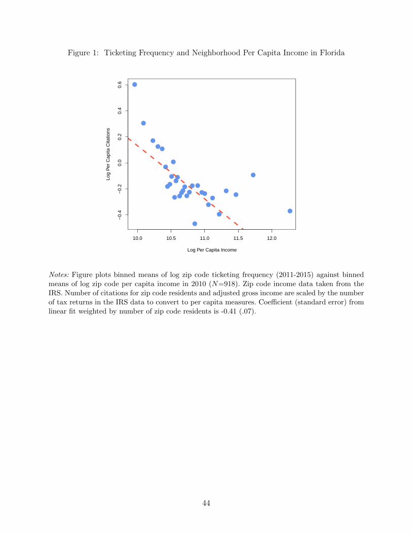
Figure 1: Ticketing Frequency and Neighborhood Per Capita Income in Florida

●

●●●

●

●●

●

●

●

●●

●●●

●

●●

●

●

●

●●

●

●

●

●●

●

●

●

10.0 10.5 11.0 11.5 12.0

−0.

4−

0.2

0.0

0.2

0.4

0.6

Log Per Capita Income

Log

Per

Cap

ita C

itatio

ns

Notes: Figure plots binned means of log zip code ticketing frequency (2011-2015) against binnedmeans of log zip code per capita income in 2010 (N=918). Zip code income data taken from theIRS. Number of citations for zip code residents and adjusted gross income are scaled by the numberof tax returns in the IRS data to convert to per capita measures. Coefficient (standard error) fromlinear fit weighted by number of zip code residents is -0.41 (.07).

44

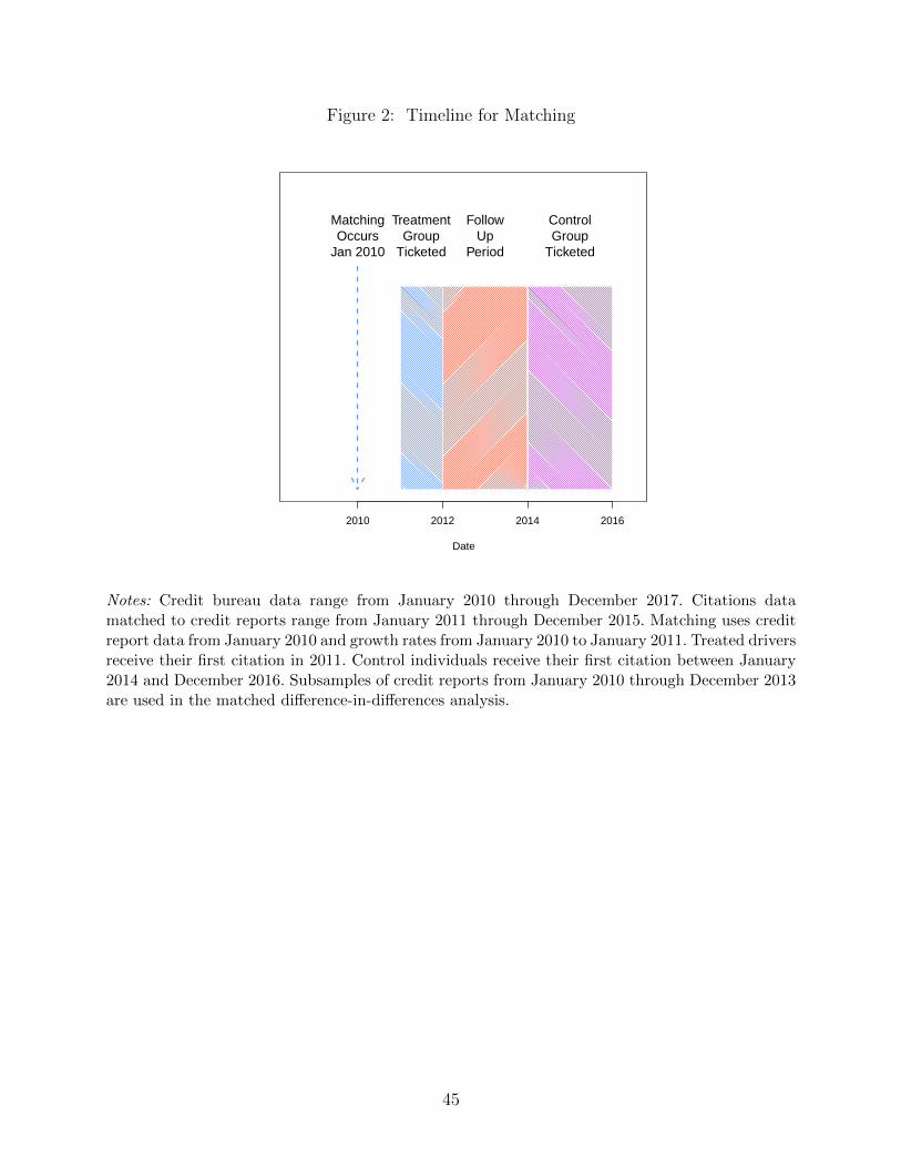
Figure 2: Timeline for Matching

●●●●●●●●●●●●●●●●●●●●●●●●●●●●●●●●●●●●●●●●●●●●●●●●●●●●●●●●●●●●●●●●●●●●●●●●●●●●●●●●●●●●●●●●●●●●●●●●

2010 2012 2014 2016

Date

MatchingOccurs

Jan 2010

TreatmentGroup

Ticketed

FollowUp

Period

ControlGroup

Ticketed

Notes: Credit bureau data range from January 2010 through December 2017. Citations datamatched to credit reports range from January 2011 through December 2015. Matching uses creditreport data from January 2010 and growth rates from January 2010 to January 2011. Treated driversreceive their first citation in 2011. Control individuals receive their first citation between January2014 and December 2016. Subsamples of credit reports from January 2010 through December 2013are used in the matched difference-in-differences analysis.

45

Figure 3: Event Study Estimates for Financial Strain Outcomes

● ● ● ● ● ● ● ● ● ● ● ● ● ● ● ● ● ● ● ● ● ● ● ● ● ● ● ● ● ● ● ● ● ● ● ● ●

−10 −5 0 5 10 15 20 25

−0.

3−

0.1

0.1

0.3

Panel A: Collections

Month Around Traffic Stop

● Full SamplePoorest Quartile

● ● ● ● ● ● ● ● ● ● ● ● ● ● ● ● ● ● ● ● ● ● ● ● ● ● ● ● ● ● ● ● ● ● ● ● ●

−10 −5 0 5 10 15 20 25−

300

−10

00

100

300

Panel B: Collections Balance

Month Around Traffic Stop

● ● ● ● ● ● ● ● ● ● ● ● ● ● ●●

●●

●●

●● ● ● ● ● ● ● ● ● ● ● ● ● ● ● ●

−10 −5 0 5 10 15 20 25

−0.

050.

000.

05

Panel C: Derogatories

Month Around Traffic Stop

● ● ● ● ● ● ● ● ● ● ● ● ● ● ● ● ● ● ● ● ● ● ● ● ● ● ● ● ● ● ● ● ● ● ● ● ●

−10 −5 0 5 10 15 20 25

−0.

06−

0.02

0.02

0.06

Panel D: Delinquencies

Month Around Traffic Stop

N otes: Figure plots event study estimates (with 95% confidence bands) for financial strain outcomesusing the event sample (710, 486 individuals). Blue circles correspond to estimates using the fullsample, while red squares correspond to estimates using the poorest quartile of drivers (estimatedincome < $21, 000). Coefficients are normalized to t = −1. All regressions include individual fixedeffects, time fixed effects, individual trends, and control for a quartic in age. Confidence bandsconstructed from standard errors clustered at the individual level.

46

Figure 4: Event Study Estimates for (Payroll) Employment

● ● ● ● ● ● ● ● ● ● ● ● ●●

●●

●●

● ● ● ● ● ● ● ● ● ● ● ● ● ● ● ● ● ● ●

−10 −5 0 5 10 15 20 25

−0.

02−

0.01

0.00

0.01

0.02

Month Around Traffic Stop

● Full SamplePoorest Quartile

N otes: Dependent variable is an indicator for positive payroll earnings (µ = 11%). Figure plotsevent study estimates (with 95% confidence bands) using the event sample (710, 486 individuals).Blue circles correspond to estimates using the full sample, while red squares correspond to estimatesusing the poorest quartile of drivers (estimated income < $21, 000). Coefficients are normalized tot = −1. All regressions include individual fixed effects, time fixed effects, individual trends, andcontrol for a quartic in age. Confidence bands constructed from standard errors clustered at theindividual level.

47

Figure 5: Event Study Estimates for Borrowing Outcomes

● ● ● ● ● ● ● ● ● ● ● ● ● ● ●●

●●

●●

●● ●

● ● ● ● ● ● ● ● ● ● ● ● ● ●

−10 −5 0 5 10 15 20 25

−0.

050.

000.

05

Panel A: Revolving Accounts

Month Around Traffic Stop

● Full SamplePoorest Quartile

●● ● ●

●● ●

● ● ● ●

●●

● ● ● ● ● ● ●

●● ● ●

● ● ● ● ● ● ● ●● ●

●● ●

−10 −5 0 5 10 15 20 25−

150

−50

050

100

Panel B: Revolving Balance

Month Around Traffic Stop

● ● ● ● ● ● ● ● ●● ●

●●

● ● ●●

●●

●●

●●

●●

●● ● ● ● ● ● ● ● ● ● ●

−10 −5 0 5 10 15 20 25

−0.

020.

000.

02

Panel C: Any Auto Loan

Month Around Traffic Stop

● ● ●●

● ● ●● ● ● ●

●● ● ● ●

● ●● ● ● ● ● ● ● ●

●● ● ● ● ● ● ● ● ● ●

−10 −5 0 5 10 15 20 25

−0.

004

0.00

00.

004

Panel D: Any Mortgage

Month Around Traffic Stop

N otes: Figure plots event study estimates (with 95% confidence bands) for borrowing outcomesusing the event sample (710, 486 individuals). Blue circles correspond to estimates using the fullsample, while red squares correspond to estimates using the poorest quartile of drivers (estimatedincome < $21, 000). Coefficients are normalized to t = −1. All regressions include individual fixedeffects, time fixed effects, individual trends, and control for a quartic in age. Confidence bandsconstructed from standard errors clustered at the individual level.

48

Figure 6: Outcomes Around Traffic Stop for Matched DD Sample (Raw Data)

−10 0 5 10 20

2.6

2.8

3.0

Panel A: Collections

Month Around Traffic Stop

●● ●

●●

●

●

●

●

●

●● ●● Treat

Control

−10 0 5 10 20

2000

2200

2400

Panel B: Collections Balance

Month Around Traffic Stop

●●

●●

●

●

●

●

●

●● ●

●

−10 0 5 10 20

1.65

1.75

1.85

Panel C: Derogatories

Month Around Traffic Stop

●

●

●

●●

●●

●●

●● ●

●

−10 0 5 10 20

0.55

0.65

0.75

Panel D: Delinquencies

Month Around Traffic Stop

● ●●

●●

●

●

●●

●

●●

●

−10 0 5 10 20

2.90

3.00

Panel E: Revolving Accounts

Month Around Traffic Stop

●

●

●

●● ● ●

●● ● ● ● ●

−10 0 5 10 20

6500

7000

7500

Panel F: Revolving Balance

Month Around Traffic Stop

●

●

●

●● ● ●

●●

●●

●●

−10 0 5 10 20

0.33

00.

345

0.36

0

Panel G: Auto Loan

Month Around Traffic Stop

●● ● ●

● ●●

● ● ● ●●

●

−10 0 5 10 20

0.26

00.

270

0.28

0

Panel H: Mortgage

Month Around Traffic Stop

●

●

● ● ● ●●

●●

●

●●

●

−10 0 5 10 20

0.11

00.

116

0.12

2

Panel I: Employment

Month Around Traffic Stop

●●

●

●

● ● ● ● ●

●

●

●

●

N otes: Figure plots averages of denoted outcome for the matched treatment (N = 333, 232) andcontrol (N = 333, 232) groups around the traffic stop date. Blue circles correspond to the treatmentgroup and red squares correspond to the control group. Treatment group means are normalized tothe control group at t = −3.

49

Figure 7: Impacts on Financial Strain by Baseline Characteristics

●

●

●

●

●

●

●

●

●

●

●

●

12 Month Treatment Effect

No Durable

Any Durable

Low Balance

High Balance

Low Collections

High Collections

Prime

Subprime

Women 35+

Women 35−

Men 35+

Men 35−

−0.03 −0.01 0.00 0.01 0.02 0.03

N otes: Figure plots estimated 12 month impacts (and 95% confidence intervals) of traffic tickets onthe financial strain index for the denoted subsamples. The financial strain index is a standardizedindex summing collections, delinquencies, and derogatory accounts. See text for additional details.Estimates obtained via difference-in-differences regressions (equation 3). Each coefficient is froma separate regression. Subprime/Prime refers to credit scores below and above 600. High/LowCollections refers to individuals with above/below median collections balances. High/Low Balancerefers to individuals with above/below median revolving balances. Any Durable refers to individualswith an open auto loan or mortgage.

50

Figure 8: Impacts on Employment by Baseline Characteristics

●

●

●

●

●

●

●

●

●

●

●

●

12 Month Treatment Effect

No Durable

Any Durable

Low Balance

High Balance

Low Collections

High Collections

Prime

Subprime

Women 35+

Women 35−

Men 35+

Men 35−

−0.015 −0.005 0.005 0.015

N otes: Figure plots estimated 12 month impacts (and 95% confidence intervals) of traffic ticketson the employment for the denoted subsamples. Employment is an indicator for having a payroll-covered job (µ = 0.16). Results using the alternate employment measure (positive payroll earnings)are nearly identical. Estimates obtained via difference-in-differences regressions (equation 3). Eachcoefficient is from a separate regression. Subprime/Prime refers to credit scores below and above600. High/Low Collections refers to individuals with above/below median collections balances.High/Low Balance refers to individuals with above/below median revolving balances. Any Durablerefers to individuals with an open auto loan or mortgage.

51

Figure 9: Treatment Effects on Strain by Baseline Financial Distress

●

●

●

●

●●

●

1 2 3 4 5 6 7

−0.

020.

000.

020.

040.

060.

080.

10

Baseline Strain Quantile

Trea

tmen

t Effe

ct

● One YearTwo Years

N otes: Figure plots estimated 12 and 24 month impacts (and 95% confidence intervals) of traf-fic tickets on financial strain (an index capturing collections, derogatories, and delinquencies) byquantiles of baseline strain. Estimates obtained via difference-in-differences regressions (equation3). Quantiles are deciles except that there is excess mass at the lower bound. Hence, quantiles2-7 correspond to the 5th-10th deciles, while quantile 1 is the bottom 40% who are approximatelyat the lower bound (i.e. individuals without collections, etc.). Regressions estimated separately byquantile group.

52

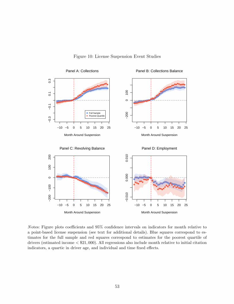
Figure 10: License Suspension Event Studies

●●●●●●●●●●●●●●●●●●●

●●●●●●●●●●●●●●●●●●

−10 −5 0 5 10 15 20 25

−0.

3−

0.1

0.1

0.3

Panel A: Collections

Month Around Suspension

● Full SamplePoorest Quartile

●●●●●●●●●●●●●●●●

●●

●●●

●●●●●●●●●●●●●●●●

−10 −5 0 5 10 15 20 25−

200

010

0

Panel B: Collections Balance

Month Around Suspension

●●●●●●●●●●●●●●●●

●●●●●●●

●●●●●●●●●●

●●

●●

−10 −5 0 5 10 15 20 25

−20

0−

100

010

020

0

Panel C: Revolving Balance

Month Around Suspension

●●●●●●●●●●●●●

●●●

●●●

●●●●●●●●●●●●●●●●

●●

−10 −5 0 5 10 15 20 25

−0.

010

0.00

00.

010

Panel D: Employment

Month Around Suspension

N otes: Figure plots coefficients and 95% confidence intervals on indicators for month relative toa point-based license suspension (see text for additional details). Blue squares correspond to es-timates for the full sample and red squares correspond to estimates for the poorest quartile ofdrivers (estimated income < $21, 000). All regressions also include month relative to initial citationindicators, a quartic in driver age, and individual and time fixed effects.

53

Table 1: Summary Statistics

Matched Suspensions

(1) (2) (3) (4) (5)Event Study Treat Control Treat Control

Panel A: DemographicsFemale 0.44 0.43 0.43 0.36 0.38Nonwhite 0.61 0.61 0.61 0.72 0.69Age 38.35 37.94 37.97 33.86 35.14Credit File Age 14.12 13.54 13.37 11.77 12.57Credit Score 609 608 609 555 573Estimated Income 31859 32901 32827 23678 25942

Panel B: Financial StrainCollections 2.81 2.75 2.58 4.02 3.64Collections Balance 2169 1998 1898 3182 2874Derogatory Accounts 1.65 1.57 1.58 1.97 1.88Delinquent Accounts 0.62 0.56 0.56 0.85 0.79Past Due Balance 4296 3750 3657 5276 5091Prior Bankruptcy 0.02 0.02 0.02 0.01 0.02

Panel C: Credit UsageAny Account 0.8 0.81 0.81 0.66 0.71Revolving Accounts 2.82 3.15 3.19 1.27 1.71Revolving Balance 6471 8663 8485 1884 2722Any Auto Loan 0.34 0.36 0.35 0.29 0.3Any Mortgage 0.25 0.28 0.28 0.11 0.14

Panel D: Payroll DataEmployed 0.16 0.16 0.16 0.15 0.16Positive Earnings 0.11 0.11 0.11 0.11 0.11Monthly Earnings 3399 3422 3566 2507 2778

Individuals 710486 333232 333232 79490 135701

N otes: Column 1 reports means for the event study sample (a random 25% sample of drivers).Columns 2-3 report means for treated and control drivers in the matched sample. See Table A-2for summary statistics for all matching candidates. Columns 5-6 report means for the driver licensesuspensions sample. See text for further details on sample construction. Summary statistics arereported as of the base period for each sample (January of the year prior to citation for the eventstudy sample, January 2010 for the matched sample, and 12 months prior to the initial citation forthe suspensions sample). As of the 2010 ACS, Florida as a whole was 51% female, 41% nonwhite,and the average age was 40.3. Statewide averages in January 2010 were 662 (credit score) and$32,000 (estimated income).

54

Table 2: Impact of Citations on Financial Strain

Event Study Matched DD

(1) (2) (3) (4) (5)Mean 12 Months 24 Months 12 Months 24 Months

Collections 2.66 0.085∗∗∗ 0.137∗∗∗ 0.075∗∗∗ 0.117∗∗∗

(0.006) (0.012) (0.009) (0.015)

Derogatories 1.74 0.038∗∗∗ 0.052∗∗∗ 0.044∗∗∗ 0.078∗∗∗

(0.004) (0.008) (0.006) (0.01)

Delinquencies 0.59 0.012∗∗∗ 0.017∗∗∗ 0.008 0.011(0.003) (0.006) (0.005) (0.008)

Index 0 0.019∗∗∗ 0.028∗∗∗ 0.018∗∗∗ 0.029∗∗∗

(0.001) (0.003) (0.002) (0.003)

Collections Balance 2111.26 75.941∗∗∗ 123.815∗∗∗ 94.069∗∗∗ 166.995∗∗∗

(8.455) (15.652) (13.842) (22.453)

Past Due Balance 4457.96 61.783∗∗ 111.996∗∗ 138.917∗∗∗ 138.496∗

(28.575) (52.139) (46.125) (75.675)

N otes: Mean in Column 1 is the control mean from the matched sample as of 3 months priorto citation. Columns 2-3 report 12 and 24 month estimates from event studies (corresponding toFigure 3). Number of individuals (observations) for event study regressions is 710,486 (34,103,328).Columns 3-4 report 12 and 24 month estimates from matched difference-in-differences regressions(corresponding to Figure 6). Number of individuals (observations) for DD regressions is 666,464(8,664,032). Index refers to the financial strain index, a standardized sum of collections, delinquen-cies, and derogatory accounts. In the event study regressions, standard errors are clustered at theindividual level. In the DD regressions, standard errors are clustered at the matched-pair level.

55

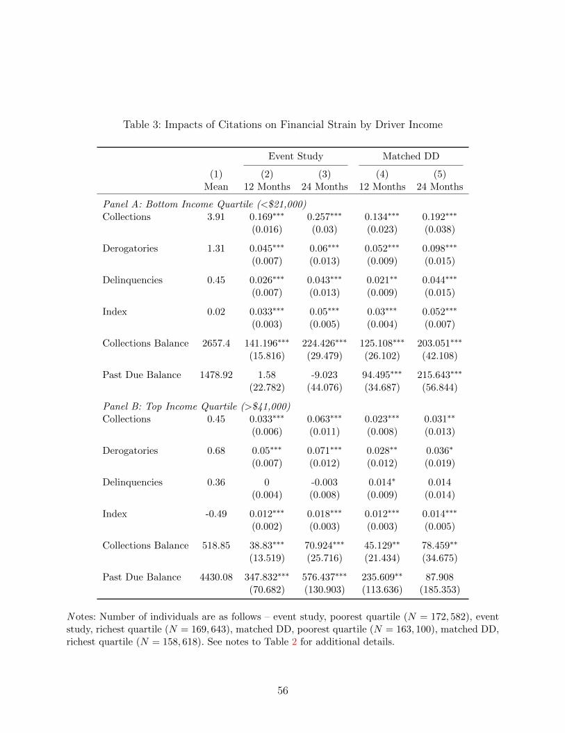
Table 3: Impacts of Citations on Financial Strain by Driver Income

Event Study Matched DD

(1) (2) (3) (4) (5)Mean 12 Months 24 Months 12 Months 24 Months

Panel A: Bottom Income Quartile (<$21,000)Collections 3.91 0.169∗∗∗ 0.257∗∗∗ 0.134∗∗∗ 0.192∗∗∗

(0.016) (0.03) (0.023) (0.038)

Derogatories 1.31 0.045∗∗∗ 0.06∗∗∗ 0.052∗∗∗ 0.098∗∗∗

(0.007) (0.013) (0.009) (0.015)

Delinquencies 0.45 0.026∗∗∗ 0.043∗∗∗ 0.021∗∗ 0.044∗∗∗

(0.007) (0.013) (0.009) (0.015)

Index 0.02 0.033∗∗∗ 0.05∗∗∗ 0.03∗∗∗ 0.052∗∗∗

(0.003) (0.005) (0.004) (0.007)

Collections Balance 2657.4 141.196∗∗∗ 224.426∗∗∗ 125.108∗∗∗ 203.051∗∗∗

(15.816) (29.479) (26.102) (42.108)

Past Due Balance 1478.92 1.58 -9.023 94.495∗∗∗ 215.643∗∗∗

(22.782) (44.076) (34.687) (56.844)

Panel B: Top Income Quartile (>$41,000)Collections 0.45 0.033∗∗∗ 0.063∗∗∗ 0.023∗∗∗ 0.031∗∗

(0.006) (0.011) (0.008) (0.013)

Derogatories 0.68 0.05∗∗∗ 0.071∗∗∗ 0.028∗∗ 0.036∗

(0.007) (0.012) (0.012) (0.019)

Delinquencies 0.36 0 -0.003 0.014∗ 0.014(0.004) (0.008) (0.009) (0.014)

Index -0.49 0.012∗∗∗ 0.018∗∗∗ 0.012∗∗∗ 0.014∗∗∗

(0.002) (0.003) (0.003) (0.005)

Collections Balance 518.85 38.83∗∗∗ 70.924∗∗∗ 45.129∗∗ 78.459∗∗

(13.519) (25.716) (21.434) (34.675)

Past Due Balance 4430.08 347.832∗∗∗ 576.437∗∗∗ 235.609∗∗ 87.908(70.682) (130.903) (113.636) (185.353)

N otes: Number of individuals are as follows – event study, poorest quartile (N = 172, 582), eventstudy, richest quartile (N = 169, 643), matched DD, poorest quartile (N = 163, 100), matched DD,richest quartile (N = 158, 618). See notes to Table 2 for additional details.

56

Table 4: Impact of Citations on Employment and Borrowing

Event Study Matched DD

(1) (2) (3) (4) (5)Mean 12 Months 24 Months 12 Months 24 Months

Employment 0.16 -0.004∗∗∗ -0.004∗∗∗ -0.005∗∗∗ -0.008∗∗∗

(0.001) (0.001) (0.001) (0.002)

Any Earnings 0.12 -0.005∗∗∗ -0.006∗∗∗ -0.005∗∗∗ -0.007∗∗∗

(0.001) (0.001) (0.001) (0.002)

Revolving Accounts 2.93 -0.037∗∗∗ -0.052∗∗∗ -0.049∗∗∗ -0.096∗∗∗

(0.004) (0.007) (0.006) (0.01)

Revolving Balance 7012.45 -33.691 -57.093 -90.98 -217.874∗∗

(25.17) (45.378) (57.02) (91.57)

Any Auto Loan 0.33 -0.007∗∗∗ -0.014∗∗∗ -0.018∗∗∗ -0.044∗∗∗

(0.001) (0.002) (0.002) (0.003)

Any Mortgage 0.27 -0.001∗ -0.002∗ -0.003∗∗∗ -0.006∗∗∗

(0.001) (0.001) (0.001) (0.002)

N otes: Mean in Column 1 is the control mean from the matched sample as of 3 months priorto citation. Columns 2-3 report 12 and 24 month estimates from event studies (corresponding toFigure 4 and Figure 5). Number of individuals (observations) for event study regressions is 710,486(34,103,328). Columns 3-4 report 12 and 24 month estimates from matched difference-in-differencesregressions (corresponding to Figure 6). Number of individuals (observations) for DD regressions is666,464 (8,664,032). In the event study regressions, standard errors are clustered at the individuallevel. In the DD regressions, standard errors are clustered at the matched-pair level.

57

Table 5: Impacts of Citations on Employment and Borrowing by Driver Income

Event Study Matched DD

(1) (2) (3) (4) (5)Mean 12 Months 24 Months 12 Months 24 Months

Panel A: Bottom Income Quartile (<$21,000)Employment 0.16 -0.009∗∗∗ -0.01∗∗∗ -0.011∗∗∗ -0.015∗∗∗

(0.002) (0.003) (0.003) (0.005)

Any Earnings 0.11 -0.009∗∗∗ -0.012∗∗∗ -0.012∗∗∗ -0.019∗∗∗

(0.002) (0.003) (0.003) (0.005)

Revolving Accounts 0.86 -0.039∗∗∗ -0.058∗∗∗ -0.042∗∗∗ -0.099∗∗∗

(0.006) (0.011) (0.008) (0.013)

Revolving Balance 412.5 7.97 -0.741 -30.313∗∗ -78.118∗∗∗

(9.476) (19.552) (13.203) (20.726)

Any Auto Loan 0.13 -0.011∗∗∗ -0.019∗∗∗ -0.02∗∗∗ -0.054∗∗∗

(0.002) (0.004) (0.003) (0.005)

Any Mortgage 0.02 -0.001 -0.002 0 -0.003∗

(0.001) (0.001) (0.001) (0.002)

Panel B: Top Income Quartile (>$41,000)Employment 0.15 -0.003∗∗ -0.004∗ -0.003∗ -0.004

(0.001) (0.002) (0.002) (0.003)

Any Earnings 0.12 -0.003∗∗∗ -0.006∗∗∗ -0.003 -0.003(0.001) (0.002) (0.002) (0.003)

Revolving Accounts 6.07 -0.029∗∗∗ -0.032∗ -0.039∗∗ -0.059∗∗

(0.009) (0.017) (0.016) (0.026)

Revolving Balance 22918.09 -120.313 -182.541 -117.946 -312.501(96.974) (175.894) (223.667) (358.718)

Any Auto Loan 0.49 -0.002 -0.004 -0.018∗∗∗ -0.035∗∗∗

(0.002) (0.004) (0.004) (0.006)

Any Mortgage 0.7 -0.003 -0.005 -0.008∗∗ -0.017∗∗∗

(0.002) (0.003) (0.003) (0.005)

N otes: Number of individuals are as follows – event study, poorest quartile (N = 172, 582), eventstudy, richest quartile (N = 169, 643), matched DD, poorest quartile (N = 163, 100), matched DD,richest quartile (N = 158, 618). See notes to Table 4 for additional details.

58

Table 6: Treatment Effects Across Studies

Studies

(1) (2) (3) (4)This Paper DFKN Herbst DGY

Panel A: Sample MeansIncome 39,000 47,000 – –Credit Score 607 731 589 581Age 37 49 43 45

Panel B: Financial Strain Effects

Collections .075 .11 – -0.15[2.8%] [12%] [-25%]

Collections Balance 94 122 – -1,315[4.5%] [10%] [-31%]

Panel C: Borrowing Effects

Revolving Accounts -.049 – .07 –[-1.7%] [2.3%]

Revolving Balance -91 -293 2,400 -920[-1.3%] [-2.5%] [17%] [-36%]

Any Auto Loan -.18 – 0 .02[-5%] [0%] [11%]

Any Mortgage -.003 – .02 .132[-1%] [10%] [36%]

Notes: DFKN refers to Dobkin et al. (2018) who study the impact of hospital admissions. Thetypical admission results in $3,275 in out-of-pocket spending. Reported estimates from DFKNcorrespond to the 12 month effects for the non-elderly insured population. Herbst refers to Herbst(2018) who studies the impact of income-driven student loan repayment, which reduces studentdebt minimum monthly payments by $140 per month on average. Reported estimates from Herbst(2018) refer to the first year DD estimates. DGY refers to Dobbie et al. (2017), who study theimpact of Chapter 13 bankruptcy protection. Effects sizes scaled by relevant baseline (i.e. percenteffects) are shown in brackets. This list is to provide context about the range of estimates in otherstudies using credit report data and is not meant to be exhaustive.

59

Table 7: Income Changes Predicting Financial Strain Impacts

Full Sample Bottom Quartile Top Quartile

(1) (2) (3) (4) (5) (6)12 Months 24 Months 12 Months 24 Months 12 Months 24 Months

Collections -361 -564 -663 -951 -144 -195[-1.05%] [-1.64%] [-3.74%] [-5.36%] [-0.25%] [-0.34%

Derogatories -250 -443 -324 -611 -208 -267[-0.73%] [-1.29%] [-1.83%] [-3.45%] [-0.36%] [-0.47%

Delinquencies -38 -52 -106 -222 -73 -73[-0.11%] [-0.15%] [-0.6%] [-1.25%] [-0.13%] [-0.13%

Index -285 -459 -465 -806 -281 -328[-0.83%] [-1.34%] [-2.62%] [-4.55%] [-0.49%] [-0.57%

N otes: Table reports an income-based metric for the matched DD treatment effects on financialstrain. Specifically, for each outcome (e.g. collections), sample (e.g. poorest quartile), and time (e.g.12 or 24 months), I estimate the income loss that would predict the treatment effect on the relevantfinancial strain using the estimates from the matched DD approach. See text for further details. Inbrackets, I report the income change as a percentage of the mean income in each subsample.

60

Table 8: Heterogeneous Impacts by Baseline Financial Situation

Baseline Credit Score Baseline Collections

(1) (2) (3) (4) (5)Full Sample Subprime Prime High Low

Collections 0.075∗∗∗ 0.1∗∗∗ 0.047∗∗∗ 0.161∗∗∗ -0.012∗

(0.009) (0.016) (0.007) (0.017) (0.007)[2.66] [4.48] [0.68] [4.29] [1.03]

Collections Balance 94.069∗∗∗ 133.211∗∗∗ 51.357∗∗∗ 200.431∗∗∗ -12.213(13.842) (24.582) (10.878) (23.939) (13.908)[2111.26] [3583.76] [504.43] [3323.54] [899.89]

Derogatories 0.044∗∗∗ 0.046∗∗∗ 0.04∗∗∗ 0.108∗∗∗ -0.021∗∗∗

(0.006) (0.01) (0.007) (0.009) (0.008)[1.74] [2.81] [0.58] [2.53] [0.96]

Delinquencies 0.008 0.001 0.015∗∗∗ -0.004 0.02∗∗∗

(0.005) (0.008) (0.006) (0.007) (0.006)[0.59] [0.86] [0.29] [0.77] [0.4]

Revolving Accounts -0.049∗∗∗ -0.04∗∗∗ -0.06∗∗∗ -0.091∗∗∗ -0.008(0.006) (0.006) (0.01) (0.007) (0.01)[2.93] [1.16] [4.86] [1.53] [4.33]

Revolving Balance -90.98 -72.554 -111.088∗∗∗ -282.195∗∗∗ 100.092(57.02) (54.52) (103.34) (48.507) (103.178)

[7012.45] [2149.66] [12318.82] [2747.69] [11274.03]

Auto Loan -0.018∗∗∗ -0.021∗∗∗ -0.014∗∗∗ -0.018∗∗∗ -0.018∗∗∗

(0.002) (0.002) (0.003) (0.002) (0.003)[0.33] [0.24] [0.44] [0.26] [0.41]

Mortgage -0.003∗∗∗ -0.002 -0.004∗∗∗ -0.002 -0.004∗∗

(0.001) (0.001) (0.002) (0.001) (0.002)[0.27] [0.13] [0.42] [0.15] [0.4]

Employment -0.005∗∗∗ -0.007∗∗∗ -0.003∗∗∗ -0.008∗∗∗ -0.003∗

(0.001) (0.002) (0.002) (0.002) (0.002)[0.16] [0.16] [0.16] [0.16] [0.16]

Individuals 666464 347768 318696 333356 333108

N otes: Table reports 12 month matched difference-in-differences estimates across subsamples. Sub-prime referes to individuals with credit scores below 600 at baseline. High collections refers toindividuals with an above median (∼ $150) collections balance at baseline.

61

Table 9: Treatment Effects of Payers and Traffic School Attendees

Unweighted Reweighted

(1) (2) (3) (4) (5)Full Sample Paid School Paid School

Strain 0.018∗∗∗ 0.0197∗∗∗ 0.0108∗ 0.0195∗∗∗ 0.0159∗∗

(0.002) (0.004) (0.006) (0.004) (0.008)

P-Value - - 0.21 - 0.67Control Mean 0 0.05 -0.16 0.01 0.01

Employment -0.0054∗∗∗ -0.0078∗∗∗ -0.0054 -0.0074∗∗∗ -0.0071(0.001) (0.002) (0.004) (0.002) (0.005)

P-Value - - 0.62 - 0.96Control Mean 0.16 0.16 0.16 0.16 0.16

Individuals 666464 198986 60288 198986 60288N 8664032 2586818 783744 2586818 783744Age 37.95 37.5 39.74 37.96 37.96Income 32.86 31.86 37.94 32.83 32.96Credit Score 609 601 644 608 609

N otes: Table reports 12 month matched difference-in-differences estimates for individuals withdispositions indicating a straight-pay and individuals with dispositions indicating a traffic schoolelection. Columns 2-3 present unweighted estimates. Column 3-4 present estimates DFL reweightingthe payer and school subsamples to replicate the baseline age × baseline income × baseline creditscore distribution of the full sample. P-values are for tests of equality between coefficients in columns2-3 and columns 3-4.

62

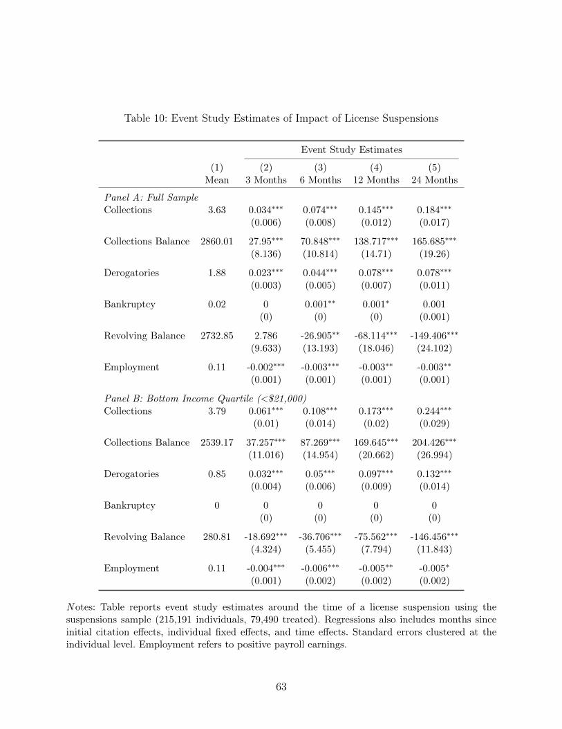
Table 10: Event Study Estimates of Impact of License Suspensions

Event Study Estimates

(1) (2) (3) (4) (5)Mean 3 Months 6 Months 12 Months 24 Months

Panel A: Full SampleCollections 3.63 0.034∗∗∗ 0.074∗∗∗ 0.145∗∗∗ 0.184∗∗∗

(0.006) (0.008) (0.012) (0.017)

Collections Balance 2860.01 27.95∗∗∗ 70.848∗∗∗ 138.717∗∗∗ 165.685∗∗∗

(8.136) (10.814) (14.71) (19.26)

Derogatories 1.88 0.023∗∗∗ 0.044∗∗∗ 0.078∗∗∗ 0.078∗∗∗

(0.003) (0.005) (0.007) (0.011)

Bankruptcy 0.02 0 0.001∗∗ 0.001∗ 0.001(0) (0) (0) (0.001)

Revolving Balance 2732.85 2.786 -26.905∗∗ -68.114∗∗∗ -149.406∗∗∗

(9.633) (13.193) (18.046) (24.102)

Employment 0.11 -0.002∗∗∗ -0.003∗∗∗ -0.003∗∗ -0.003∗∗

(0.001) (0.001) (0.001) (0.001)

Panel B: Bottom Income Quartile (<$21,000)Collections 3.79 0.061∗∗∗ 0.108∗∗∗ 0.173∗∗∗ 0.244∗∗∗

(0.01) (0.014) (0.02) (0.029)

Collections Balance 2539.17 37.257∗∗∗ 87.269∗∗∗ 169.645∗∗∗ 204.426∗∗∗

(11.016) (14.954) (20.662) (26.994)

Derogatories 0.85 0.032∗∗∗ 0.05∗∗∗ 0.097∗∗∗ 0.132∗∗∗

(0.004) (0.006) (0.009) (0.014)

Bankruptcy 0 0 0 0 0(0) (0) (0) (0)

Revolving Balance 280.81 -18.692∗∗∗ -36.706∗∗∗ -75.562∗∗∗ -146.456∗∗∗

(4.324) (5.455) (7.794) (11.843)

Employment 0.11 -0.004∗∗∗ -0.006∗∗∗ -0.005∗∗ -0.005∗

(0.001) (0.002) (0.002) (0.002)

N otes: Table reports event study estimates around the time of a license suspension using thesuspensions sample (215,191 individuals, 79,490 treated). Regressions also includes months sinceinitial citation effects, individual fixed effects, and time effects. Standard errors clustered at theindividual level. Employment refers to positive payroll earnings.

63

A Appendix Figures and Tables

Figure A-1: Local Policing Intensity and Per Capita Income in the U.S.

●

●

●

●●

●●

●

●

●

●

●●

●

●

●

●

●●●

●

●

●

●

●

●

●

●

●

●

10.2 10.4 10.6 10.8 11.0 11.2

−6.

3−

6.2

−6.

1−

6.0

Log Per Capita Income

Log

Per

Cap

ita S

wor

n O

ffice

rs

Notes: Figure plots binned means of log sworn officers per capita against binned means of log localper capita income using a 2010 cross-section from the sample of municipal police departments inMello (2018) (N = 4, 327). Dashed line is a linear fit. Coefficient (standard error) from linear fit is-0.24 (.03).

64

Figure A-2: Reliance on Fines and Fees and Per Capita Income in the U.S.

●

●

●

●

●

●

●

●

●

●

●

●

●

●

●

●

●●●

●●

●●

●

●

● ●

●

●

●

9.5 10.0 10.5 11.0

1.5

2.0

2.5

3.0

Log Per Capita Income

Per

cent

Loc

al R

even

ue fr

om F

ines

Notes: Figure plots local means of the fraction of local revenue generated from fines and fees againstlocal means of log per capita income using the data from Sances & You (2017) (N = 9, 142). Dashedline is a linear fit. Coefficient (standard error) from the implied regression is -0.6 (0.09).

65

Figure A-3: Credit File Match Rate by Zip Code Per Capita Income

●

●

●

●

●

●●

●

●

●

●

●

●

●

●

●

●

●●

●

●

●

●

●

●

●

●

●●

●

10.0 10.5 11.0 11.5 12.0

0.78

0.80

0.82

0.84

0.86

Log Per Capita Income

Mat

ch R

ate

N otes: Figure plots local means of the match rate (fraction of citations matched to the credit file)against the log per capita income of the driver’s home zip code computed from the IRS public usefiles. Sample is the universe of citations sent to credit bureau (N = 8, 851, 688). Dashed line is alinear fit. Coefficient (standard error) from the implied regression is 0.035 (0.003).

66

Figure A-4: Correlation Between Estimated Income and Payroll Earnings

●●●●●●●●●●●● ● ●

●●

●●

●

●

0 20 40 60 80 100

020

4060

8010

0

Annualized Earnings (Payroll Data)

Est

imat

ed In

com

e (C

redi

t Dat

a)

N otes: Figure plots local means of estimated income against annual earnings in the payroll data asof January 2010. Sample is individuals in the matched sample with positive payroll earnings at thatdate (N = 69, 548). Red dashed line is a linear fit. Coefficient (standard error) from the impliedregression is 0.3515 (0.0023). Purple dashed line is the 45-degree line.

67

Figure A-5: Age Profiles for Select Outcomes

20 30 40 50 60

580

620

660

Credit Score

Age

20 30 40 50 60

1525

3545

Estimated Income

Age

20 30 40 50 60

01

23

Collections

Age

20 30 40 50 60

010

0020

00

Collections Balance

Age

20 30 40 50 60

12

34

56

Revolving Accounts

Age

20 30 40 50 60

010

000

2000

0

Revolving Balance

Age

20 30 40 50 60

0.05

0.20

0.35

Auto Loan

Age

20 30 40 50 60

0.0

0.2

0.4

Mortgage

Age

20 30 40 50 60

0.10

0.14

0.18

Employment

Age

N otes: Figure plots the cross-sectional age profiles in January 2010 for selected outcomes usingcited drivers present in the credit report data as of that date using ages 18-64 (N = 2, 720, 749).

68

Figure A-6: Event Study Estimates without Individual Trends

●●●●●●●●●●●●●●●●●●●●●●●●●●●●●●●●●●●●●

−10 0 5 10 20

−0.

3−

0.1

0.1

0.3

Panel A: Collections

Month Around Traffic Stop

● Full SamplePoorest Quartile

●●●●●●●●●●●●●●●●●●●●●●●●●●●●●●●●●●●●●

−10 0 5 10 20

−30

0−

100

100

300

Panel B: Collections Balance

Month Around Traffic Stop

●●●●●●●●●●●●●●●●●

●●●●●●●●●●●●●●●●●●●●

−10 0 5 10 20

−0.

050.

05

Panel C: Derogatories

Month Around Traffic Stop

●●●●●●●●●●●●●●●●●●●●●●●●●●●●●●●●●●●●●

−10 0 5 10 20

−0.

050.

05

Panel D: Delinquencies

Month Around Traffic Stop

●●●●●●●●●●●●●●●●●●●●●●●●●●●●●●●●●●●●●

−10 0 5 10 20

−0.

100.

000.

10

Panel E: Revolving Accounts

Month Around Traffic Stop

●●

●●●

●●●●●●

●●

●●●●●●●●●●●●●●●●●●●

●●●●●

−10 0 5 10 20

−10

00

50

Panel F: Revolving Balance

Month Around Traffic Stop

●●●●●●●●●●●●

●●●●●●●●●●●●●●●●●●●●●●●●●

−10 0 5 10 20

−0.

030.

000.

03

Panel G: Auto Loan

Month Around Traffic Stop

●●●●●●●●●●●●●●●●●●

●●●●●●●●●●●●●●●●●●●

−10 0 5 10 20

−0.

004

0.00

00.

004

Panel H: Mortgage

Month Around Traffic Stop

●●●●●●●●●●●●●●●●●●●●●●●●●●●●●●●●●●●●●

−10 0 5 10 20

−0.

020.

000.

02

Panel I: Employment

Month Around Traffic Stop

N otes: Figure plots coefficients (with 95% confidence bands) from event study regressions. Coef-ficients are normalized to t = −1. Blue circles correspond to estimates using the full sample andRed squares correspond to estimates using the poorest quartile. Identical to Figure 3, Figure 4, andFigure 5 except that regressions do not include individual trends.

69

Figure A-7: Event Study Estimates for Monthly Earnings

● ●●

●● ● ●

● ● ● ● ● ● ●

● ●● ● ●

● ● ● ● ●● ●

● ●● ●

●●

● ●● ● ●

−10 −5 0 5 10 15 20 25

−0.

06−

0.04

−0.

020.

000.

020.

040.

06

Month Around Traffic Stop

● Full SamplePoorest Quartile

N otes: Dependent variable is a log monthly earnings from the payroll data. Figure plots eventstudy estimates (with 95% confidence bands) using individuals from the event sample ever havingpositive earnings (N = 191, 054). Coefficients are normalized to t = −1. All regressions includeindividual fixed effects and time effects.

70

Figure A-8: Fully Non-Parametric Matched Difference-in-Differences Estimates

● ● ● ● ● ● ● ● ● ● ● ● ●

−10 0 5 10 20

−0.

30.

00.

2

Collections

Month Around Traffic Stop

● Full SampleBottom Income QuartileTop Income Quartile

● ● ● ● ● ● ● ●● ● ● ● ●

−10 0 5 10 20−

300

−10

010

030

0

Collections Balance

Month Around Traffic Stop

● ● ● ● ● ● ●● ● ● ● ● ●

−10 0 5 10 20

−0.

150.

000.

10

Derogatories

Month Around Traffic Stop

● ● ● ● ● ● ● ● ● ● ● ● ●

−10 0 5 10 20

−0.

050.

05

Delinquencies

Month Around Traffic Stop

● ● ● ● ● ● ●●

● ●●

● ●

−10 0 5 10 20

−0.

150.

000.

10

Revolving Accounts

Month Around Traffic Stop

● ● ● ● ● ● ● ● ● ● ● ● ●

−10 0 5 10 20−

1000

050

0

Revolving Balance

Month Around Traffic Stop

● ●●

●● ●

●●

●●

●●

●

−10 0 5 10 20

−0.

030.

000.

02

Any Auto

Month Around Traffic Stop

● ● ● ● ● ● ● ● ● ● ● ● ●

−10 0 5 10 20

−0.

020.

000.

02

Any Mortgage

Month Around Traffic Stop

● ● ● ● ●● ● ● ● ● ● ● ●

−10 0 5 10 20

−0.

015

0.00

00.

015

Employment

Month Around Traffic Stop

N otes: Figure plots coefficients (95% confidence intervals) on interactions between a treatmentindicator and event time indicators, normalized to equal zero at t = 3, corresponding to equation(2). All regressions include event time fixed effects, individual fixed effects, and year and monthfixed effects. Standard errors are clustered at the matched pair-level. Blue circles are estimatesusing the full matched sample, red squares are estimates using the poorest quartile of drivers, andpurple diamonds are estimates using the richest quartile of the sample. Each series (outcome ×sample) is from a separate regression.

71

Figure A-9: Employment Effects by Baseline Employment Status

−10 −5 0 5 10 15 20 25

0.6

0.7

0.8

0.9

1.0

Panel A: Employed

Month Around Traffic Stop

●

●

●

●

●

●●

●●

●●

●●

● TreatControl

−10 −5 0 5 10 15 20 250.

240.

280.

32

Panel B: Employed (Poor)

Month Around Traffic Stop

●

●

●

●●

●●

●●

●●

●●

−10 −5 0 5 10 15 20 25

0.00

0.02

0.04

0.06

Panel C: Not Employed

Month Around Traffic Stop

●

●

●

●

●●

●●

● ● ● ● ●

−10 −5 0 5 10 15 20 25

0.03

0.05

0.07

Panel D: Not Employed (Poor)

Month Around Traffic Stop

●

●

●

●

●●

●●

● ● ● ● ●

N otes: Figure plots mean employment rates (covered by payroll data) around the time of a trafficstop for the treatment and control groups (analogous to Figure 6), splitting the sample by baselineemployment status. Blue dots denote the treatment group and red dots denote the control group.Treatment group means normalized to control group at t = −3. Panels A and C plot means for thefull sample, while Panels B and D plot means for the poorest quartile of drivers.

72

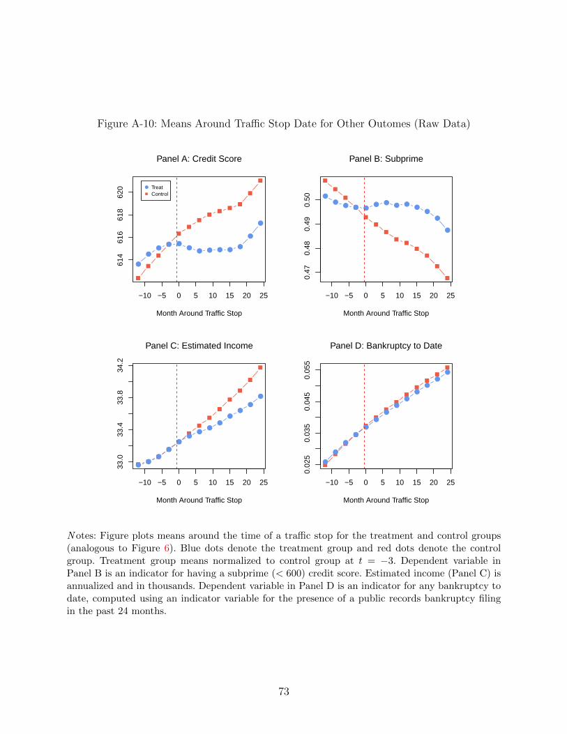
Figure A-10: Means Around Traffic Stop Date for Other Outomes (Raw Data)

−10 −5 0 5 10 15 20 25

614

616

618

620

Panel A: Credit Score

Month Around Traffic Stop

●

●●

● ●●

● ● ● ●●

●

●

● TreatControl

−10 −5 0 5 10 15 20 25

0.47

0.48

0.49

0.50

Panel B: Subprime

Month Around Traffic Stop

●●

● ● ●● ● ● ●

●●

●

●

−10 −5 0 5 10 15 20 25

33.0

33.4

33.8

34.2

Panel C: Estimated Income

Month Around Traffic Stop

●●

●

●

●●

●●

●●

●●

●

−10 −5 0 5 10 15 20 25

0.02

50.

035

0.04

50.

055

Panel D: Bankruptcy to Date

Month Around Traffic Stop

●

●

●

●

●

●

●●

●

●●

●●

N otes: Figure plots means around the time of a traffic stop for the treatment and control groups(analogous to Figure 6). Blue dots denote the treatment group and red dots denote the controlgroup. Treatment group means normalized to control group at t = −3. Dependent variable inPanel B is an indicator for having a subprime (< 600) credit score. Estimated income (Panel C) isannualized and in thousands. Dependent variable in Panel D is an indicator for any bankruptcy todate, computed using an indicator variable for the presence of a public records bankruptcy filingin the past 24 months.

73

Figure A-11: Outcome Means Using All Match Candidates

−10 0 5 10 20

2.6

2.8

3.0

Collections

Month Around Traffic Stop

●● ●

●●

●

●

●

●

●

●● ●

−10 0 5 10 20

1900

2100

2300

2500

Collections Balance

Month Around Traffic Stop

●●

●●

●

●

●

●

●●

● ●●

−10 0 5 10 20

1.60

1.70

1.80

Derogatories

Month Around Traffic Stop

●

●

●

●●

●●

●●

● ● ●●

−10 0 5 10 20

0.55

0.65

0.75

Delinquencies

Month Around Traffic Stop

● ●●

●●

●

●

●

●

●●

●●

−10 0 5 10 20

3.05

3.15

Revolving Accounts

Month Around Traffic Stop

●

●

●

●●

● ●●

● ● ● ● ●

−10 0 5 10 20

6800

7400

8000

Revolving Balance

Month Around Traffic Stop

●

●

●

●● ● ●

●●

●●

●●

−10 0 5 10 20

0.33

50.

350

0.36

5

Any Auto Loan

Month Around Traffic Stop

●● ● ● ●

●●

● ● ● ●●

●

−10 0 5 10 20

0.28

00.

290

Any Mortgage

Month Around Traffic Stop

●

●

●● ● ●

●●

●●

●●

●

−10 0 5 10 20

0.15

40.

158

Employment

Month Around Traffic Stop

●●

●

●●

● ● ● ●●

●

●

●

N otes: Figure plots means of outcomes for treatment and control groups using all match candidates(N=1,430,723). Blue dots denote the treatment group and red squares denote the control group.Treatment groups means normalized to equal control group means at t = −3. Placebo traffic stopdates are assigned to the control group randomly to replicate the distribution of traffic stop datesin the treatment group.

74

Figure A-12: Imputed Fine Gradients

●

●●

●●

0 50 100 200 300

−0.

050.

050.

150.

25

Panel A: Collections

Imputed Fine

● Full SampleBottom Income Quartile

●

●

●

●●

0 50 100 200 300

−50

5015

025

0

Panel B: Collections Balance

Imputed Fine

●

●

●

●

●

0 50 100 200 300

−0.

10−

0.06

−0.

020.

02

Panel C: Revolving Accounts

Imputed Fine

●

●

●

●

●

0 50 100 200 300

−40

00

200

Panel D: Revolving Balance

Imputed Fine

N otes: Figure plots 12 month matched difference-in-differences estimates (and 95% confidenceintervals) separately by quintile of imputed fine for the treatment group’s citation. Blue circlescorrespond to estimates using the full sample, while red squares correspond to estimates using onlythe bottom income quartile.

75

Figure A-13: Effects by Common Violation Types

●

●

●

●

●

●

●

Panel A: Strain Index

Treatment Effect

SDL

Equipment

Toll

Tag

RLC

Seatbelt

Speed

−0.08 −0.04 0.00 0.04 0.08

(21,532)

(29,601)

(29,558)

(35,625)

(33,593)

(30,600)

(38,646)

●

●

●

●

●

●

●

Panel B: Employment

Treatment Effect

SDL

Equipment

Toll

Tag

RLC

Seatbelt

Speed

−0.0100 −0.0025 0.0025 0.0075

N otes: Figure plots 12 month matched difference-in-differences estimates by violation type for com-mon violation categories. SDL refers to driving with a suspended license. Numbers in parenthesesare average estimated income (in thousands) and credit score at baseline for the relevant sample.

76

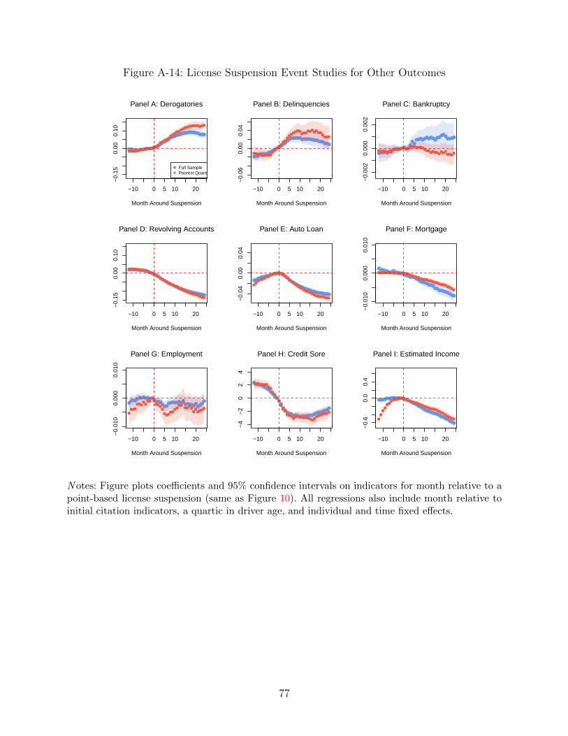
Figure A-14: License Suspension Event Studies for Other Outcomes

●●●●●●●●●●●●●●●●●●●●●●●●●●●●●●●●●●●●●

−10 0 5 10 20

−0.

150.

000.

10

Panel A: Derogatories

Month Around Suspension

● Full SamplePoorest Quartile

●●●●●●●●●●●●●●●●●●●●●●●●●●●●●●●●●●●●●

−10 0 5 10 20

−0.

060.

000.

04

Panel B: Delinquencies

Month Around Suspension

●●●●●●●●●●●●●●●

●●

●●●●●●●●●●●

●●●●

●●●●●

−10 0 5 10 20

−0.

002

0.00

00.

002

Panel C: Bankruptcy

Month Around Suspension

●●●●●●●●●●●●●●●●●●●●●●●●●●●●●●●●●●●●●

−10 0 5 10 20

−0.

150.

000.

10

Panel D: Revolving Accounts

Month Around Suspension

●●●●●●●●●●●●●●●●●●●●●●●●●●●●●●●●●●●●●

−10 0 5 10 20

−0.

040.

000.

04

Panel E: Auto Loan

Month Around Suspension

●●●●●●●●●●●●●●●●●●●●●●●●●●●●●

●●●●●●●●

−10 0 5 10 20

−0.

010

0.00

00.

010

Panel F: Mortgage

Month Around Suspension

●●●●●●●●●●●●●

●●●●

●●●●●●●●●●

●●●●●●

●●●

●

−10 0 5 10 20

−0.

010

0.00

00.

010

Panel G: Employment

Month Around Suspension

●●●●●●●●●

●●

●●

●●

●●●●●●●●●●●●●●●●●●●●●●

−10 0 5 10 20

−4

−2

02

4

Panel H: Credit Sore

Month Around Suspension

●●●●●●●●●●●●●●●●●●●●●●●●●●●●●●●●●●●●●

−10 0 5 10 20

−0.

60.

00.

4

Panel I: Estimated Income

Month Around Suspension

N otes: Figure plots coefficients and 95% confidence intervals on indicators for month relative to apoint-based license suspension (same as Figure 10). All regressions also include month relative toinitial citation indicators, a quartic in driver age, and individual and time fixed effects.

77

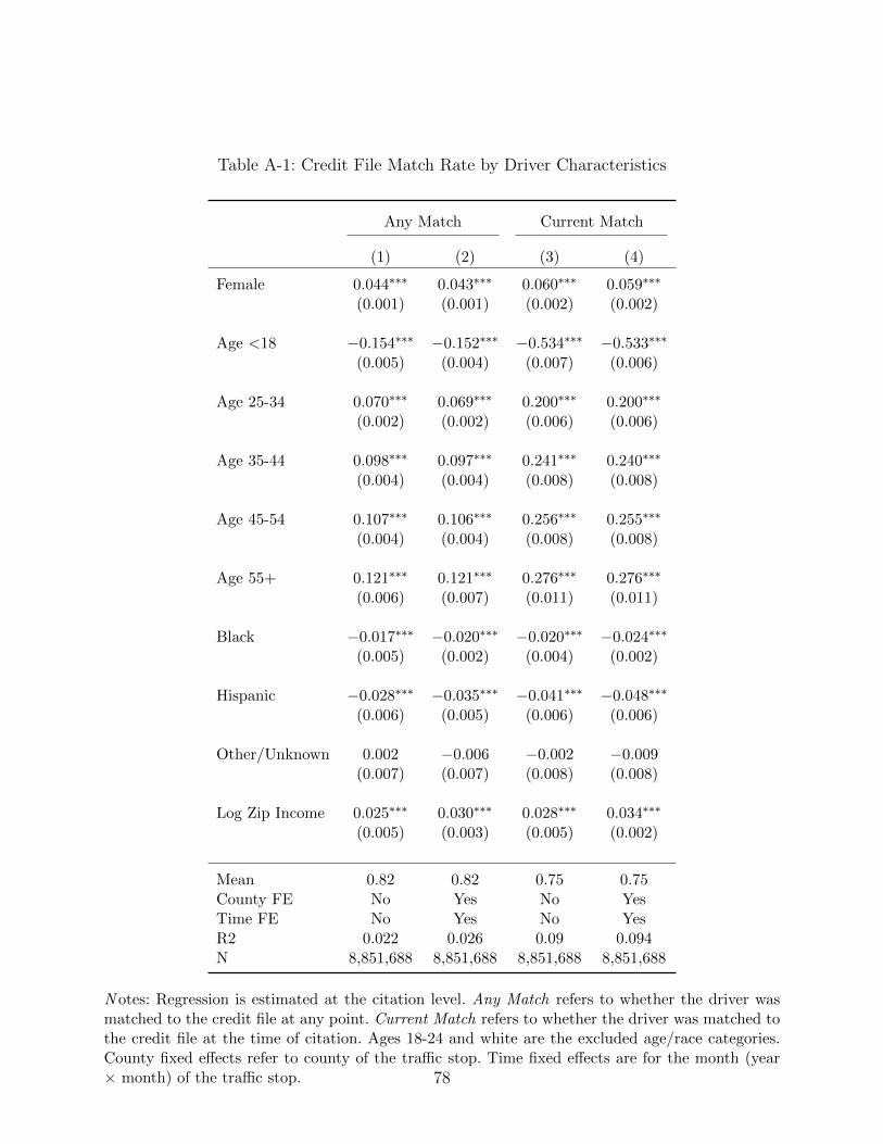
Table A-1: Credit File Match Rate by Driver Characteristics

Any Match Current Match

(1) (2) (3) (4)

Female 0.044∗∗∗ 0.043∗∗∗ 0.060∗∗∗ 0.059∗∗∗

(0.001) (0.001) (0.002) (0.002)

Age <18 −0.154∗∗∗ −0.152∗∗∗ −0.534∗∗∗ −0.533∗∗∗

(0.005) (0.004) (0.007) (0.006)

Age 25-34 0.070∗∗∗ 0.069∗∗∗ 0.200∗∗∗ 0.200∗∗∗

(0.002) (0.002) (0.006) (0.006)

Age 35-44 0.098∗∗∗ 0.097∗∗∗ 0.241∗∗∗ 0.240∗∗∗

(0.004) (0.004) (0.008) (0.008)

Age 45-54 0.107∗∗∗ 0.106∗∗∗ 0.256∗∗∗ 0.255∗∗∗

(0.004) (0.004) (0.008) (0.008)

Age 55+ 0.121∗∗∗ 0.121∗∗∗ 0.276∗∗∗ 0.276∗∗∗

(0.006) (0.007) (0.011) (0.011)

Black −0.017∗∗∗ −0.020∗∗∗ −0.020∗∗∗ −0.024∗∗∗

(0.005) (0.002) (0.004) (0.002)

Hispanic −0.028∗∗∗ −0.035∗∗∗ −0.041∗∗∗ −0.048∗∗∗

(0.006) (0.005) (0.006) (0.006)

Other/Unknown 0.002 −0.006 −0.002 −0.009(0.007) (0.007) (0.008) (0.008)

Log Zip Income 0.025∗∗∗ 0.030∗∗∗ 0.028∗∗∗ 0.034∗∗∗

(0.005) (0.003) (0.005) (0.002)

Mean 0.82 0.82 0.75 0.75County FE No Yes No YesTime FE No Yes No YesR2 0.022 0.026 0.09 0.094N 8,851,688 8,851,688 8,851,688 8,851,688

N otes: Regression is estimated at the citation level. Any Match refers to whether the driver wasmatched to the credit file at any point. Current Match refers to whether the driver was matched tothe credit file at the time of citation. Ages 18-24 and white are the excluded age/race categories.County fixed effects refer to county of the traffic stop. Time fixed effects are for the month (year× month) of the traffic stop. 78

Table A-2: Summary Statistics for Matching Candidates and Matches

Candidates Matches

(1) (2) (3) (4) (5)Treat Control Treat Control Statewide

Panel A: DemographicsFemale 0.4 0.45 0.43 0.43 0.51Nonwhite 0.65 0.53 0.61 0.61 0.41Age 36.96 38.65 37.94 37.97 40.3Credit File Age 13 13.94 13.54 13.37 -Credit Score 597 616 608 609 662Estimated Income 31323 33788 32901 32827 32000

Panel B: Financial StrainCollections 2.95 2.58 2.75 2.58 -Collections Balance 2139 1846 1998 1898 -Derogatory Accounts 1.68 1.53 1.57 1.58 -Delinquent Accounts 0.6 0.54 0.56 0.56 -Past Due Balance 4092 3479 3750 3657 -Prior Bankruptcy 0.02 0.02 0.02 0.02 -

Panel C: Credit UsageAny Account 0.8 0.82 0.81 0.81 -Revolving Accounts 2.85 3.32 3.15 3.19 -Revolving Balance 7802 8929 8663 8485 -Any Auto Loan 0.35 0.36 0.36 0.35 -Any Mortgage 0.26 0.3 0.28 0.28 -

Panel D: Payroll DataEmployed 0.16 0.15 0.16 0.16 -Positive Earnings 0.11 0.11 0.11 0.11 -Monthly Earnings 3203 3612 3422 3566 -

Individuals 817775 612948 333232 333232 -

N otes: Candidates refers to individuals eligible for the matching procedure. Matches refers toindividuals successfully matched. Benchmark values for demographic characteristics computed fromthe 2010 ACS. Benchmark values for credit score and estimated income were provided by the creditbureau.

79

Table A-3: Difference in Difference Estimates for Other Outcomes

(1) (2) (3) (4)Credit Score Subprime Estimated Income Bankruptcy

Panel A: Full Sample

12 Months Post -1.452∗∗∗ 0.006∗∗∗ -186.988∗∗∗ 0(0.25) (0.002) (34.353) (0)

24 Months Post -0.106 0.001 -385.384∗∗∗ 0.001(0.39) (0.003) (54.384) (0.001)

Control Mean 615.38 0.5 33154.02 0.03Individuals 666464 666464 666464 666464N 8641126 8641126 8664025 8664032

Panel B: Bottom Income Quartile (<$21,000)

12 Months Post -2.33∗∗∗ 0.01∗∗∗ 6.055 0(0.532) (0.003) (38.949) (0)

24 Months Post -2.3∗∗∗ 0.01∗ -203.058∗∗∗ 0(0.825) (0.005) (61.563) (0.001)

Control Mean 556.62 0.73 16517.7 0.01Individuals 163100 163100 163100 163100N 2108433 2108433 2120295 2120300

Panel C: Top Income Quartile (>$41,000)

12 Months Post -0.909∗ 0.002 -507.786∗∗∗ 0.001(0.49) (0.003) (114.526) (0.001)

24 Months Post 0.835 -0.007 -871.389∗∗∗ 0.003(0.767) (0.005) (181.841) (0.002)

Control Mean 711.46 0.15 57946.12 0.02Individuals 158618 158618 158618 158618N 2060092 2060092 2062034 2062034

N otes: Table presents matched differences-in-differences estimates (same as columns 4-5 in Table 3)for other outcomes. Dependent variable in column 2 is an indicator for having a subprime (< 600)credit score. Dependent variable in column 4 is any bankruptcy to date, constructed from a variableindicating the presence of a public records bankruptcy filing in the past 24 months. Note thatcredit score and estimated income variables are not imputed and hence missing person-months aredropped.

80

Table A-4: Difference-in-Differences Estimates for Employment and Earnings

Full Sample Positive Earnings

(1) (2) (3) (4)Employed Any Earnings Earnings Log Earnings

Panel A: Full Sample

12 Months Post -0.005∗∗∗ -0.005∗∗∗ -126.103 -0.004(0.001) (0.001) (78.933) (0.009)

24 Months Post -0.008∗∗∗ -0.007∗∗∗ -112.557 -0.007(0.002) (0.002) (131.556) (0.014)

Control Mean 0.16 0.12 3697 7.74Individuals 666464 666464 146141 146141N 8664032 8664032 1015962 1015962

Panel B: Bottom Income Quartile (<$21,000)

12 Months Post -0.011∗∗∗ -0.012∗∗∗ -52.391∗ -0.027(0.003) (0.003) (30.16) (0.022)

24 Months Post -0.015∗∗∗ -0.019∗∗∗ -3.251 -0.041(0.005) (0.005) (69.609) (0.035)

Control Mean 0.16 0.11 1611 7.1Individuals 163100 163100 44652 44652N 2120300 2120300 244051 244051

Panel C: Top Income Quartile (>$41,000)

12 Months Post -0.003∗ -0.003 -279.688 0.004(0.002) (0.002) (192.022) (0.015)

24 Months Post -0.004 -0.003 -425.991 -0.002(0.003) (0.003) (309.955) (0.024)

Control Mean 0.15 0.12 6926 8.39Individuals 158618 158618 27284 27284N 2062034 2062034 241762 241762

N otes: Table presents matched differences-in-differences estimates (same as columns 4-5 in Table 3)for employment and earnings.

81

Table A-5: Sensitivity of 12 Month Effects to Imputation

Data Type

(1) (2)Imputed Not Imputed

Panel A: Financial StrainCollections 0.075∗∗∗ 0.079∗∗∗

(0.009) (0.009)Derogatories 0.044∗∗∗ 0.047∗∗∗

(0.006) (0.006)Collections Balance 94∗∗∗ 94∗∗∗

(14) (14)Past Due Balance 139∗∗∗ 148∗∗∗

(46) (48)

Panel B: Credit UsageRevolving Accounts -0.049∗∗∗ -0.051∗∗∗

(0.006) (0.007)Revolving Balance -91 -58

(57) (109)Any Auto Loan -0.018∗∗∗ -0.022∗∗∗

(0.002) (0.002)Any Mortgage -0.003∗∗∗ -0.003

(0.001) (0.002)

N otes: Table presents 12 month matched difference-in-differences estimates (standard errors inparentheses) with and without data imputation. Column 1 reports estimates identical to those inTable 2 and Table 4.

82

B Becker-Style Model

B-1 Model Environment

The model is based on the canonical model of the economics of crime in Becker (1968) andfollows closely the formulation in Burlando & Motta (2016). Society is comprised of a unitmass of individuals indexed by their endowed income y and taste for crime x. I assumethat income is exogenous, and to start, homogenous in the population. Taste for crime x isdistributed according to the cumulative distribution function G(·). Individuals have strictlyconcave utility over consumption u(c) and receive utility x from (successfully) committingcrime.

Each criminal act causes harm to society. Hence, the government tries to curb crimethrough an enforcement scheme θ = (p, f), where p represents the probability a citizen isaudited and f denotes the fine paid by an individual found to be engaging in crime. Takingthe enforcement scheme as given, individuals choose whether to engage in crime to maximizeexpected utility. Hence, individuals choose crime if

pu(y − f) + (1− p) [u(y) + x]︸ ︷︷ ︸expected utility for criminals

> u(y)︸︷︷︸utility for abstainers

(B.1)

Equation B.1 determines a threshold value of x as a function of y and θ:

x∗(y, p, f) =p

1− p[u(y)− u(y − f)] (B.2)

Individuals with x > x∗ engage in crime, while those with x ≤ x∗ abstain. Given y and θ,the amount of crime is 1−G(x∗(y, θ)). One can think of this expression as a demand curve,mapping the (expected) price of crime to the quantity of offenses.

It is also useful to note that given y and θ, total welfare of citizens can be expressed as

V (y, θ) =

∫ x∗

0

u(y)g(x)dx+

∫ ∞x∗

{pu(y − f) + (1− p) [u(y) + x]

}g(x)dx (B.3)

which is the utility of abstainers and criminals integrated over the distribution of x.

B-2 Enforcement and Welfare

Before turning to policy discussion, it is useful to note that policy analysis in this Becker-style model will require an understanding of the relationship between welfare V and theenforcement scheme θ. In particular, one needs to differentiate V with respect to the policyparameters p and f . Taking y as given and beginning at the enforcement scheme θ0 = (p0, f0),consider a small change in one of the policy parameters moving to θ1.

With respect to a policy change, there are three distinct types of citizens. First, there isa group of never-takers. Never-takers are individuals who abstain from crime regardless ofthe enforcement scheme, i.e. individuals with x ≤ x1. If the policy change is, for example, anincrease in p, then x1 = x∗(y, p0, f0). Second, there is a group or always-takers. Always-takersare citizens who choose crime regardless of the enforcement scheme, i.e. individuals with

83

x > x2, where x2 = x∗(y, p1, f0) for an increase in p. Finally, there is a group of compliers.Compliers are individuals with x ∈ (x1, x2], and therefore whose behavior is altered by thepolicy change. For an increase in p, compliers are individuals who choose crime under θ0 butabstain under θ1. Hence, the welfare change associated with a small policy change can beexpressed as∫ x1

0

[∂u

∂θ|x ≤ x1

]g(x)dx+

∫ x2

x1

[∂u

∂θ|x ∈ (x1, x2]

]g(x)dx+

∫ ∞x2

[∂u

∂θ|x > x2

]g(x)dx (B.4)

The first term is the change in utility for the never-takers. Because such individuals abstainregardless, they receive u(y) under either θ. There is no welfare change for never-takers,meaning the first term is zero.

The second term is the welfare change for the compliers. Such individuals were marginalto abstaining under θ0 and choose to abstain under θ1. By the envelope theorem, there is nowelfare change for compliers. The second term is zero.

The third term is the welfare change for the always-takers. Policy parameters do impactthe expected payoff associated with crime, thereby affecting the expected utility of the in-framarginal criminals. Hence, given tht the first two terms are zero, the only welfare impactsof a small change in enforcement are the effects on inframarginal criminals:

∂V

∂θ=

∫ ∞x2

∂

∂θ

{pu(y − f) + (1− p) [u(y) + x]

}g(x)dx (B.5)

The following discussion below makes use of this result.

B-3 Optimal Enforcement

The government chooses an enforcement scheme to maximize the welfare of citizens, net ofthe social costs of crime and the costs of enforcement. For simplicity, assume the governmenttakes the fine f as given and chooses only p. This assumption captures the fact that, in manycases, fines are set at the state or county-level but policing intensity is chosen locally.26

To begin with a reduced-form version of the planner’s problem, let h(p) represent thesocial cost of crime as a function of p and let c(p) denote the cost of policing. One could thinkof this formulation as expressing that only the government cares about crime or that victim-ization costs are evenly distributed throughout the population. The government’s problemis

maxp

V (p)− h(p)− c(p) (B.6)

Under standard regularity conditions, the solution is characterized by the first-order condi-

26Standard Becker-style models typically assume that increasing the number of searches is costlybut increasing the charged fine is not, which leads to the prediction of much higher fines than aregenerally observed in cases such as traffic enforcement. Assuming the government takes the fineas given is isomorphic to assuming there is maximum acceptable fine amount f̄ , reflecting fairnessconcerns for example, because optimization will always dictate f = f̄ .

84

tion−h′(p)︸ ︷︷ ︸

marginal safety benefit

= c′(p)︸︷︷︸marginal cost of policing

− V ′(p)︸ ︷︷ ︸marginal welfare loss

(B.7)

In words, the government tickets until the marginal safety benefit equals the marginal costof writing tickets and the marginal lost surplus to citizens. It is worth noting that if thegovernment also faces a revenue-raising motive when issuing citations, this would enter thefirst-order condition as a constant on the left-hand side of B.7. With a revenue benefit, thegovernment is willing to allow a larger welfare loss to citizens when optimizing.

Using B.5, the marginal welfare loss associated with increasing p, V ′(p) is

∂V

∂p=

∫ ∞x∗

[u(y − f)− u(y)− x

]g(x)dx (B.8)

This expression depends on the utility losses associated with punishment and the benefits tocriminal behavior. To obtain a more tractable expression, one can think of a small increasein p as writing one more traffic ticket. Moreover, assume that the marginal person ticketedwas close to the margin of criminal behavior. Hence, we can substitute the indifference x∗

condition into the derivative of the expected utility of criminals to get the marginal welfareloss associated with one more ticket is

1

1− p[u(y − f)− u(y)

](B.9)

Assuming p is small, then, optimal enforcement sets

u(y)− u(y − f) = −h′(p)− c′(p) (B.10)

We can think of the left-hand side of B.10 as a reduced-form expression of the quantityestimated in the data, the welfare cost of punishing an individual.

B-4 Income-Based Fines

Now suppose that society is comprised of types of individuals, those with high incomes yHand those with low incomes yL, where yH > yL. Assume taste for crime x is distributedidentically across the two types of individuals. I examine the effect of moving from an initialenforcement scheme θ0 = (p0, f0) to a small perturbation in the fines for the two types.Specifically, I consider an increase in the fine for rich individuals to fH = f0 + ∆ and adecrease in the fine for rich individuals to fL = f0 −∆, where ∆ > 0.

To simplify the exposition, let ∆ satisfy the following condition:

x∗(yH , p, f0 + ∆) = x∗(yL, p, f0) (B.11)

The relevance of this assumption is as follows.27 Recall from section B-2 that, for small ∆,

27To see that such a ∆ exists, note that by the definition x∗, ∆ solves u(yL) − u(yL − f0) =u(yH)−u(yH−f0−∆). The properties of u(·) dictate that u(yL)−u(yL−f0) > u(yH)−u(yH−f0)and that u(yH)− u(yH − f0 −∆) is increasing in ∆.

85

we need only consider the utility implications for the always-takers when evaluating welfareeffects. When moving from f0 to f0 + ∆, the always-takers among the rich are those withx > x∗(yH , p, f0 + ∆), or those who engage in crime when f is either f0 or f + ∆. Whenmoving from f0 to f0−∆, the always-takers among the poor are those with x > x∗(yL, p, f0).Hence, B.11 ensures that the distribution of x’s among the rich and poor always-takers areidentical, allowing for a simpler expression of welfare effect that abstracts from compositionalchanges.

Equation B.5 shows that the derivative of the expected utility of criminals with respectto the relevant enforcement parameter is a key object in evaluating welfare effects. Withrespect to fine changes, this quantity is

∂

∂f{pu(y − f) + (1− p) [u(y) + x]} = −p∂u

∂c(y − f) < 0 (B.12)

Substituting B.12 into B.5 gives the following expression for the net welfare change associatedwith the change in the fine scheme:∫ ∞

x∗(yL,f0,p)

∆p∂u

∂c(yL − f0)g(x)dx+

∫ ∞x∗(yH ,f0+∆,p)

−∆p∂u

∂c(yH − f0)g(x)dx (B.13)

where the first term is the welfare change among poor always-takers and the second termis the welfare change among rich always-takers. Using assumption B.11, which ensures thatthe limits of integration are equal, this expression can be rewritten as

∆×[∂u

∂c(yL − f0)− ∂u

∂c(yH − f0)

]︸ ︷︷ ︸

difference in marginal utilities

× p[1−G(x∗)]︸ ︷︷ ︸number of tickets

(B.14)

The first and last components are positive by assumption and definition. Strict concavityof u(·) ensures that the difference in marginal utilities is positive, and therefore, that thewelfare change is positive.

To obtain a money metric for the welfare changes, I rescale by marginal utility at thelow income level (Chetty, 2006a).28 For a CRRA utility function with risk aversion γ, themoney-metric welfare change is

(yL − f0)−γ − (yH − f0)−γ

y−γL×∆× p[1−G(x∗)] (B.15)

To relate this expression to the paper’s empirical exercise, let yL =$20,000, yH =$40,000,and f0 =$200. One of the main insights offered by the empirical analysis is the fact thatfines have outsized effects on the utility of poor drivers. To incorporate this finding intothe welfare analysis in a reduced-form way, let e capture the excess burden of fines on poordrivers. We can think of this quantity as the “effective” fine size, corresponding to the welfarecost estimates in Section 6. Taking this heterogeneity into account, the change-in-welfare

28The unit of the welfare change is change in utils. Multiplying by one over the marginal utilityscales by the price of a util, i.e. converts the change in utility into dollar units.

86

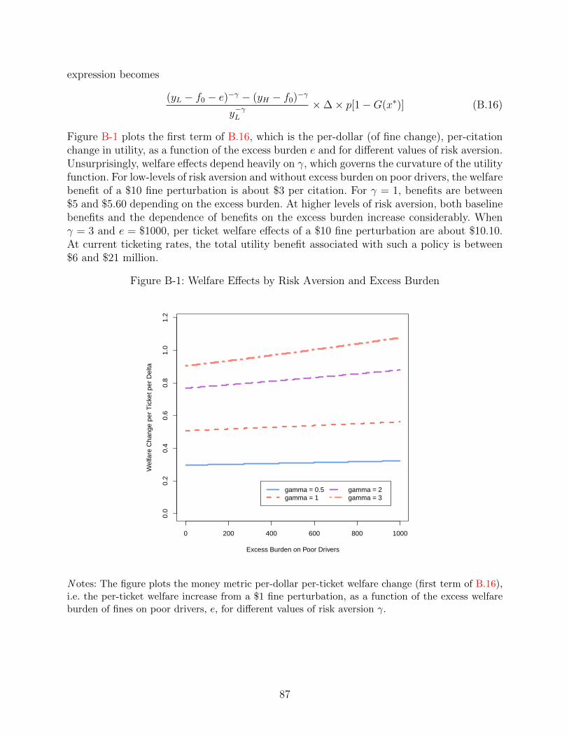
expression becomes

(yL − f0 − e)−γ − (yH − f0)−γ

y−γL×∆× p[1−G(x∗)] (B.16)

Figure B-1 plots the first term of B.16, which is the per-dollar (of fine change), per-citationchange in utility, as a function of the excess burden e and for different values of risk aversion.Unsurprisingly, welfare effects depend heavily on γ, which governs the curvature of the utilityfunction. For low-levels of risk aversion and without excess burden on poor drivers, the welfarebenefit of a $10 fine perturbation is about $3 per citation. For γ = 1, benefits are between$5 and $5.60 depending on the excess burden. At higher levels of risk aversion, both baselinebenefits and the dependence of benefits on the excess burden increase considerably. Whenγ = 3 and e = $1000, per ticket welfare effects of a $10 fine perturbation are about $10.10.At current ticketing rates, the total utility benefit associated with such a policy is between$6 and $21 million.

Figure B-1: Welfare Effects by Risk Aversion and Excess Burden

0 200 400 600 800 1000

0.0

0.2

0.4

0.6

0.8

1.0

1.2

Excess Burden on Poor Drivers

Wel

fare

Cha

nge

per

Tic

ket p

er D

elta

gamma = 0.5gamma = 1

gamma = 2gamma = 3

N otes: The figure plots the money metric per-dollar per-ticket welfare change (first term of B.16),i.e. the per-ticket welfare increase from a $1 fine perturbation, as a function of the excess welfareburden of fines on poor drivers, e, for different values of risk aversion γ.

87

Impacts on Crime

Of course, the net social welfare implications of the policy change also depends on the policy’seffects on crime and/or revenue from fines. Note that for a given y and enforcement regimeθ, the amount of crime is C = 1−G(x∗(y, θ)). Hence, crime changes with f according to

∂C

∂f= −g(x∗)× p

1− p× ∂u

∂c(y − f) (B.17)

where the expression beginning with p1−p follows from differentiating x∗ with respect to f .

The income-based fine regime increases (decreases) the price of crime for the rich (poor),thus decreasing crime among rich individuals but increasing crime among poor individuals.The net effect of the policy on crime can be expressed as

∆p

1− p

[g(x∗(yL, p, f0))

∂u

∂c(yL − f0)− g(x∗(yH , p, f0))

∂u

∂c(yH − f0)

](B.18)

The first term inside the brackets represents in the increase in crime for the poor and thesecond term represents the decline for the rich. While concavity of u(·) ensures that u′(yL−f0) > u′(yH − f0) and x∗0(yL) > x∗0(yH), the sign of B.18 depends on the functional form ofg(·), or more specifically the shape of the distribution of crime tastes in the range of thecutoff values. If x has a strictly decreasing probability distribution function (an exponentialdistribution, for example), the policy increases crime. If g(·) is increasing in the range of theinitial x∗ values, the policy could reduce crime.

An important point to note is that the above analysis of welfare changes relies on aspecific magnitude of ∆ to simplify the exposition. However, one could also have chosen analternate fine scheme specifically to hold crime constant. The redistributive welfare benefitswould still be present under such an alternative policy, but one would also need to considerchanges in the composition of criminals and the associated welfare implications.

88

C Effects of Payroll-Job Separations

In this section, I estimate the impact of a separation from a payroll-covered job on creditreport outcomes. This exercise serves two distinct purposes. First, it provides a test of thehypothesis that payroll employment is a meaningful and positive outcome. Second, to theextent that a separation impacts credit report outcomes, the estimates can be used as abenchmark to help interpret the magnitudes of the estimated traffic ticket effects.

C-1 Sample Construction

To isolate the impacts of separations unrelated to traffic citations, I sample from the set ofindividuals who receive their first traffic ticket after January 2014 and analyze data from Jan-uary 2010 through 2013. I drop individuals included in the matched difference-in-differencessample, require that individuals are present in the credit file in January 2010, and requirethat individuals are between 18 and 60 years of age as of that date.

I then identify individuals with a separation from the payroll data during in 2011 or 2012,measured as a transition from having at least one covered job to having zero covered jobsin adjacent months. Requiring that the separation occurs in the 2011-2012 period allows abalanced 12-month period before and after the separation for analysis and allows for thecomputation of a crude tenure measure. That is, using the one-year pre-period, I can at leastdistinguish between spells of, e.g., three months and spells of longer than twelve months.There are 26,718 individuals meeting all the above requirements. To help estimate time andage effects, I include individuals meeting the same criteria but whose payroll employmentspells begin after 2013 as a quasi-control group. There are 38,345 such individuals.

Table C-1 presents summary statistics for the separations sample. The treatment (sepa-rations) and control groups are quite similar on most dimensions. Compared with the eventstudy and matched difference-in-differences samples, this group of drivers is a higher fractionfemale and slightly younger, but otherwise similar on most dimensions.

C-2 Estimation

To estimate the impacts of separations, I use an event-study approach. Specifically, I estimateregressions of the following form:

Yitτ =∑τ

θτ + φi + κt + γi(t) + εit (C.1)

Here, the θτ ’s are month around separation indicators and φi and κt are individual and timefixed effects. I group event-time values larger than +/-13 into +/-13. I also include individual-specific linear trends γi(t) in the regressions. Finally, I control for a quartic in driver age andinclude a set of job tenure indicators, which are indicators for number of months since thepayroll employment spell began, topcoded at twelve because this is the longest look-backperiod allowed for the universe of separations. Event-time and tenure indicators are set tozero for the control group. I cluster standard errors at the individual-level.

89

C-3 Results

Table C-1: Summary Statistics for Job Separations Sample

(1) (2)Separations Control

Panel A: DemographicsFemale 0.51 0.52Nonwhite 0.47 0.49Age 34.7 35.15Credit File Age 11.85 12.13Credit Score 600 599Estimated Income 28746 28972

Panel B: Financial StrainCollections 3.01 3.03Collections Balance 1991 2010Derogatory Accounts 1.59 1.56Delinquent Accounts 0.53 0.55Past Due Balance 2793 2881Prior Bankruptcy 0.02 0.02

Panel C: Credit UsageAny Account 0.78 0.77Revolving Accounts 2.63 2.63Revolving Balance 5302 5376Any Auto Loan 0.32 0.32Any Mortgage 0.23 0.24

Individuals 26718 38345

N otes: The table reports summary statistics for the event-study analysis of payroll job separations.Columnn 1 reports means as of January 2010 for individuals with a separation in 2011-2012 andcolumn 2 reports means as of January 2010 for control individuals (those with a spell in the payrolldata after January 2014). See notes to Table 1 for further details.

90

Figure C-1: Effect of Payroll Separations on Financial Strain

(a) Collections

●● ● ● ●

● ● ● ● ● ● ●●

● ● ●

●

●

●

●

●

● ●●

●

−10 −5 0 5 10

−0.

15−

0.10

−0.

050.

000.

050.

100.

15

Month Around Separation

● b(12)=0.114

(b) Collections Balance

●

● ●●

● ●

●● ● ●

● ●●

● ●●

●

●

●

● ●

● ●● ●

−10 −5 0 5 10

−10

0−

500

5010

0

Month Around Separation

● b(12)=70

(c) Derogatories

●● ● ● ● ● ●

●● ●

●●

●●

● ●

●● ●

●●

● ●

● ●

−10 −5 0 5 10

−0.

06−

0.04

−0.

020.

000.

020.

040.

06

Month Around Separation

● b(12)=0.038

(d) Delinquencies

● ● ●

●● ●

●● ●

● ● ●● ●

●

●

●

●

●●

●●

●●

●

−10 −5 0 5 10

−0.

04−

0.02

0.00

0.02

0.04

Month Around Separation

● b(12)=0.02

N otes: Each figure plots coefficients and 95% confidence intervals on month around payroll sep-aration indicators. Regressions also include individual and time fixed effects, payroll tenure fixedeffects, a quartic in age, and individual-specific linear trends. Standard errors are clustered at theindividual level. The average separation corresponds to a $1,600 decline in monthly payroll earnings.Legend reports the 12-month estimate.

91

Figure C-2: Effect of Payroll Separations on Credit Cards

(a) Revolving Accounts

●

● ●● ● ● ●

● ● ●●

● ●● ●

●● ●

●

●

●

●●

● ●

−10 −5 0 5 10

−0.

04−

0.02

0.00

0.02

0.04

Month Around Separation

● b(12)=−0.027

(b) Revolving Balance

●●

●● ● ●

●● ●

● ●● ● ●

●●

●● ● ●

●

● ●●

●

−10 −5 0 5 10

−40

0−

200

020

040

0

Month Around Separation

● b(12)=−280

N otes: Each figure plots coefficients and 95% confidence intervals on month around payroll sep-aration indicators. Regressions also include individual and time fixed effects, payroll tenure fixedeffects, a quartic in age, and individual-specific linear trends. Standard errors are clustered at theindividual level. The average separation corresponds to a $1,600 decline in monthly payroll earnings.Legend reports the 12-month estimate.

92