Spectral Methods for Uncertainty Quantification · us to implement the spectral collocation method...
190
Spectral Methods for Uncertainty Quantification Christian Brams Kongens Lyngby 2013 DTU Compute - B.Sc.Eng.- 2013- 3
Transcript of Spectral Methods for Uncertainty Quantification · us to implement the spectral collocation method...

Spectral Methods for UncertaintyQuantification
Christian Brams
Kongens Lyngby 2013DTU Compute - B.Sc.Eng.- 2013- 3
Technical University of DenmarkDepartment of Applied Mathematics and Computer ScienceMatematiktorvet, building 303B, DK-2800 Kongens Lyngby, DenmarkPhone +45 [email protected] DTU Compute - B.Sc.Eng.- 2013- 3
Summary (English)
The goal of the thesis is to apply uncertainty quantification by generalized poly-nomial chaos with spectral methods on systems of partial differential equations,and implement the methods in the Python programming language.
We start off by introducing the mathematical basis for spectral methods for nu-merical computations. Deriving standard forms of differential operators enableus to implement the spectral collocation method on most partial differentialequations. We implement the spectral methods in Python, creating a stan-dardized method for solving a numerical problem spectrally using the spectralcollocation method.
Afterwards we derive the stochastic collocation and Galerkin methods, allowingus to combine the spectral methods with the generalized polynomial chaos meth-ods in order to achieve exponential convergence in both the numerical solutionas well as the quantification of uncertainty.
Using Python as the medium, we implement these combined methods on a liddriven cavity problem as well as a two dimensional tank with nonlinear freesurface movement, in order to examine the impact uncertainty on the inputcan have on a system of partial differential equations, and how to efficientlyquantify the impact. It is discovered that using uncertainty quantification, wecan describe the actual effect of the variables, by looking at what changes whenthe variable is subject to uncertainty, even for nonlinear systems.
The methods derived in this thesis combine excellently, and are easy to im-plement on most partial differential equations, allowing great versatility in im-

ii
plementing these methods of uncertainty quantification on different differentialsystems.

Summary (Danish)
Formålet med denne opgave er at anvende kvantificering af usikkerhed ved meto-den generalized polynomial chaos sammen med spektrale metoder til løsning afpartielle differentialligninger, og at implmenetere dette i programmeringssprogetPython.
Vi starter med at indtroducere den matematiske basis for spektrale metodertil numeriske beregninger. Ved at udlede standardiserede udtryk for differenti-al operatorer, kan vi implementere spektral kollokations metoden på de flestepartielle differential systemer. Vi implementerer de spektrale metoder i Python,og opsætter en standardiseret metode til at løse numeriske problemer med denspektrale kollokations metode.
Herefter udledes stokastisk kollokations og Galerkin metoder, hvilket tilladeros at kombinere spektral metoder med stokastise generalized polynomial chaosmetoder, til at opnå eksponentiel konvergens både på den numeriske løsning ogi kvantificeringen af usikkerhed i et system.
Ved at anvende Python, implementerer vi disse metoder sammen på et lid drivencavity problem og en simuleret to-dimensionel vandtank med ikke-lineær fri over-fladebevægelse. Med udgangspunkt i disse to problemstillinger vil vi undersøgebetydningen af usikkerhed på input i et system af partielle differentialligninger,og hvordan man effektivt kvantificerer dette. Det viser sig at man kan sige me-get om en enkelt konstants indflydelse på et system, ved at analysere hvordanusikkerhed på denne konstant påvirker systemet.
Metoderne der er udledt i denne opgave kan med fordel kombineres og nemt

iv
anvendes på det fleste partielle differentialligninger, hvilket giver stor mulighedfor anvendelse til kvantificering af usikkerhed på forskellige differentiallignings-systemer.

Preface
This thesis was prepared at the department of Applied Mathematics and Com-puter Science at the Technical University of Denmark in fulfillment of the re-quirements for acquiring an B.Sc.Eng. in Mathematics and Technology.
The thesis deals with Spectral Methods, and the application regarding Uncer-tainty Qualification.
The thesis consists of a study of spectral methods, their application and imple-mentation in the Python programming language. It contains a chapter explor-ing the method of generalized polynomial chaos (GPC) for use with uncertaintyquantification. The goal of this thesis is to be able to combine the spectralmethods with the GPC methods for uncertainty quantification, in order to cre-ate an efficient way to quantify the propagation of uncertainty through partialdifferential equation models.
In order to fully comprehend this thesis, it is assumed that the reader has basicknowledge of numerical methods for solving differential equations, as well as anunderstanding of linear algebra and programming on a basic level.
Lyngby, 31-January-2013
Christian Brams

vi

Acknowledgements
I would like to thank my supervisor Allan P. Engsig-Karup and Ph.D. studentDaniele Bigoni for their invaluable help during this project. Without theircounseling and guidance, I would likely never have finished the project.
Additionally, I would like to thank Charlotte Frausing for having an near inex-haustible reservoir of smiles and help whenever I needed it.
I would like to thank my family for providing understanding and support, as wellas relieving me of some of the more menial tasks when the deadline approached.
Kenneth, Anna and Christine deserve a special thanks, for providing a forumwith intelligent feedback, when we first endeavored into spectral methods.

viii

Contents
Summary (English) i
Summary (Danish) iii
Preface v
Acknowledgements vii
1 Introduction 1
2 Problem statement 3
3 Spectral methods as numerical methods 53.1 Orthogonal polynomials . . . . . . . . . . . . . . . . . . . . . . . 5
3.1.1 Generating the polynomials . . . . . . . . . . . . . . . . . 63.1.2 Differentiating the polynomials . . . . . . . . . . . . . . . 113.1.3 Challenges for discrete modeling . . . . . . . . . . . . . . 13
3.2 Constructing spectral solvers . . . . . . . . . . . . . . . . . . . . 153.2.1 Spectral methods . . . . . . . . . . . . . . . . . . . . . . . 153.2.2 Types of differential equation problems . . . . . . . . . . 17
3.3 Solving differential equations . . . . . . . . . . . . . . . . . . . . 183.3.1 Using the spectral collocation method . . . . . . . . . . . 183.3.2 Burgers’ equation . . . . . . . . . . . . . . . . . . . . . . . 19
4 Implementation of spectral methods 214.1 How to use Python for numerical computations . . . . . . . . . . 21
4.1.1 A comparison to MATLAB . . . . . . . . . . . . . . . . . . . 224.1.2 Employed Python packages . . . . . . . . . . . . . . . . . 23
4.2 Challenges using Python instead of MATLAB . . . . . . . . . . . . 25

x CONTENTS
4.2.1 Integer division . . . . . . . . . . . . . . . . . . . . . . . . 254.2.2 Interfacing with MATLAB . . . . . . . . . . . . . . . . . . . 264.2.3 Python overhead . . . . . . . . . . . . . . . . . . . . . . . 26
4.3 Implementation for spectral methods . . . . . . . . . . . . . . . . 274.3.1 Generating the differential operators . . . . . . . . . . . . 274.3.2 Employing the time-stepping method . . . . . . . . . . . . 304.3.3 Handling multi-dimensional problems . . . . . . . . . . . 314.3.4 Sparse matrices . . . . . . . . . . . . . . . . . . . . . . . . 34
4.4 Practical implementation . . . . . . . . . . . . . . . . . . . . . . 344.4.1 Implementing the spectral collocation method . . . . . . . 354.4.2 Burgers’ equation – implementing the solver . . . . . . . . 36
5 Stochastic formulation and uncertainty quantification 395.1 Probability theory . . . . . . . . . . . . . . . . . . . . . . . . . . 39
5.1.1 Basic concepts . . . . . . . . . . . . . . . . . . . . . . . . 405.1.2 How to formulate a stochastic problem . . . . . . . . . . . 425.1.3 Calculating the expectation . . . . . . . . . . . . . . . . . 44
5.2 Quantification of uncertainty . . . . . . . . . . . . . . . . . . . . 455.3 Sampling methods . . . . . . . . . . . . . . . . . . . . . . . . . . 46
5.3.1 Non-intrusive methods . . . . . . . . . . . . . . . . . . . . 465.3.2 Intrusive methods . . . . . . . . . . . . . . . . . . . . . . 48
5.4 Examples of uncertainty quantification . . . . . . . . . . . . . . . 495.4.1 The test equation – stochastic collocation method . . . . 495.4.2 The test equation – stochastic Galerkin method . . . . . . 535.4.3 Burgers’ equation – the influence of uncertainty . . . . . . 565.4.4 The test equation – two dimensional uncertainty . . . . . 59
6 Numerical experiments 616.1 Lid driven cavity . . . . . . . . . . . . . . . . . . . . . . . . . . . 61
6.1.1 Derivation of the spectral model . . . . . . . . . . . . . . 626.1.2 Implementation of the spectral model . . . . . . . . . . . 666.1.3 Introducing uncertainty on the Reynolds number . . . . . 716.1.4 Numerical experiments with UQ on the Reynolds number 726.1.5 Conclusions for the lid driven cavity flow model . . . . . . 80
6.2 A nonlinear 2D wave tank model . . . . . . . . . . . . . . . . . . 806.2.1 Derivation of the spectral model . . . . . . . . . . . . . . 826.2.2 Implementation of the spectral model . . . . . . . . . . . 846.2.3 Introducing uncertainty into the amplitude . . . . . . . . 906.2.4 Numerical experiments with uncertainty . . . . . . . . . . 916.2.5 Conclusions for the wave tank model . . . . . . . . . . . . 94
7 Conclusions 97

CONTENTS xi
A Conventions for notation and plotting 99A.1 Differential notation . . . . . . . . . . . . . . . . . . . . . . . . . 99A.2 Uncertainty quantification in plots . . . . . . . . . . . . . . . . . 99A.3 Coding notation . . . . . . . . . . . . . . . . . . . . . . . . . . . 100
B Allan P. Engsig-Karup, notes 101
C Code used in chapter 3 103C.1 Generating plots . . . . . . . . . . . . . . . . . . . . . . . . . . . 103
D Code used in chapter 4 109D.1 Differential Matrices . . . . . . . . . . . . . . . . . . . . . . . . . 109D.2 Test functions . . . . . . . . . . . . . . . . . . . . . . . . . . . . . 110
D.2.1 The test for the two-dimensional differential . . . . . . . . 113D.2.2 The test for the sparse matrices speed . . . . . . . . . . . 115
D.3 Practical implementations . . . . . . . . . . . . . . . . . . . . . . 116
E Code used in chapter 5 121E.1 Visualization . . . . . . . . . . . . . . . . . . . . . . . . . . . . . 121E.2 Practical examples . . . . . . . . . . . . . . . . . . . . . . . . . . 122
E.2.1 Test equation . . . . . . . . . . . . . . . . . . . . . . . . . 122E.2.2 Burgers’ equation . . . . . . . . . . . . . . . . . . . . . . . 133
F Code used in the lid driven cavity problem 141F.1 Approximating solution . . . . . . . . . . . . . . . . . . . . . . . 141F.2 Visualizing . . . . . . . . . . . . . . . . . . . . . . . . . . . . . . 156
G Code used in the 2D wave tank problem 161G.1 Time-integration functions . . . . . . . . . . . . . . . . . . . . . . 161G.2 Problem implementations . . . . . . . . . . . . . . . . . . . . . . 166
Bibliography 175

xii CONTENTS

Chapter 1
Introduction
Uncertainty quantification is the concept of characterizing the effects of un-certainty to a useable domain. This allows us to quantify the effects a slightchange in the input will have when applied to an advanced mathematical model.This characterization is applicable to most areas of science, as it is infeasible toreplicate the exact conditions for the tests which are run.
Through David A. Kopriva’s "Implementing Spectral Methods for Partial Differ-ential Equations", [Kop09], this thesis will explore the numerical spectral meth-ods used for solving differential equations. This will allow for rapid convergencein the error for the numerical solutions to differential equations, enabling us tosample data with lesser points.
Implementing these numerical methods is essential to the process, as the vastamounts of calculations needed to be done is insurmountable to anything butcomputers. For this we will explore the possibilities for implementing thesemethods in an open and easily acceptable form, through the programming lan-guage of Python. Using the communally developed packages SciPy and NumPy,we can emulate the easy and optimized interface of MATLAB, without the need forcommercial licenses, allowing everyone to utilize the ideas behind these methods.
Using Dongbin Xiu’s "Numerical Methods for Stochastic Computations", un-certainty quantification will be introduced, with the main focus on generalized

2 Introduction
polynomial chaos, a method with very fast convergence in the errors of quan-tifying uncertainty, akin to the spectral methods described in Kopriva’s book.Generalized polynomial chaos is currently "one of the most widely adoptedmethods, and in many cases the only feasible method, for stochastic simulationsof complex systems" as Xiu explains in his preface.
Combining the spectral methods with the generalized polynomial chaos meth-ods, we will create accurate methods for solving partial differential equations,while quantifying the uncertainty propagated through the models, by uncer-tainty on the boundary or initial conditions. This will allow us to effectivelyexamine the impact of uncertainty on complex differential models.

Chapter 2
Problem statement
The main goal of the thesis is to
1. Be able to describe and understand relevant theory, from spectral methodsto uncertainty quantification.
2. Develop routines and spectral solvers in Python.
3. Exemplify uncertainty quantification techniques through application withdifferent equation solvers.
4. Formulate and express a clear set of hypotheses and project aims.
5. Conceive, design and execute appropriate experiments, analytical and/ormodeling methods.
6. Communicate knowledge through well written, well presented, concise,clear and well structured reports and oral presentations. Present projectresults using clear tables and figures.
7. Understand the interaction between the different components of a techno-logical issue.

4 Problem statement
Chapter 3
Spectral methods asnumerical methods
Spectral methods are numerical methods designed for solving ordinary differen-tial equations (ODEs) or partial differential equations (PDEs) as well as otherrelated problems. The basic idea behind spectral methods can be compared tothe finite element methods, where the solution is found as a function of the basisfunctions representing the spectrum. The key difference is that for finite elementmethods, the basis functions are zero on large parts of the domain, while forspectral methods the basis functions are typically nonzero. This gives the func-tions excellent error properties for smooth functions, as the error is minimizedacross the spectrum, allowing exponential convergence.
3.1 Orthogonal polynomials
Orthogonal polynomials are the basis of the spectral methods. The orthogonal-ity property allow us to find a unique set of coefficients to describe our function,and it is central to the concept of spectral methods. The idea of the spec-tral methods lie in approximating the function using a finite sum of orthogonalpolynomials.
6 Spectral methods as numerical methods
Any function ϕ(x, t) can be represented as a sum of a unique set of coefficientspaired with the appropriate orthogonal basis from the family of basis functionsΦn(x)∞n=0 such that
ϕ(x, t) =
∞∑k=0
ϕk(t)Φk(x)
This assumes that the basis functions are orthogonal on an interval [a, b], withrespect to a weight function w, such that
(Φn,Φm)w =
∫ b
a
Φn(x)Φ∗m(x)w(x) dx = Cnδnm δnm
1, n = m
0, n 6= m(3.1)
Another central aspect of the polynomials we will be using, will be that theyhave an associated easy to evaluate quadrature, which is used to approximatethe integral of the functions.
Q[f ] =
N∑j=0
f(xj)wj =
∫ b
a
f(x) dx+E
3.1.1 Generating the polynomials
The main classes of polynomials we will be using are the Lagrange polynomials,for periodic functions using Fourier interpolation, and the Legendre polynomials,for use with non-periodic functions.
3.1.1.1 Periodic functions
For periodic functions, we will be using a Fourier series to approximate our func-tions, since these will have an inherent periodicity – allowing us to exploit this toautomatically ensure periodicity. In essence, any function can be approximatedby a Fourier series, but since we want to truncate the function and not includethe infinite sum, we will only use the Fourier basis for periodic functions. Thefunction F is approximated by the infinite sum
f(x) =
∞∑k=−∞
fkeikx

3.1 Orthogonal polynomials 7
Since the complex exponentials – the Fourier basis functions – are orthogonal,(3.1) makes it easy to calculate the Fourier coefficients fk.
(FN , e
inx)
=
( ∞∑k=−∞
fkeikx, einx
)=
∞∑k=−∞
fk(eikx, einx
)= Cnfn
Where the weights can be calculated to w = 2π, since the basis functions are2π-periodic
Cn =(einx, einx
)=
∫ 2π
0
ei(n−n)x dx = 2π
This relies on infinite sums, and to be able to compute this, we need to truncatethe function, letting us have a truncated function Pnf(x)
PNf(x) =
N/2∑k=−N/2
fkeikx
The error between PNf and f is shown in [Kop09, eq. 1.30] to be directlyrelated to the size of the remaining coefficients. This allows the spectral methodsto obtain exponential convergence for functions where the coefficients decreaseexponentially – functions periodic on [0, 2π] with all derivatives continuous.
A special case of this exists, called INf the Fourier interpolant, where we com-pute the coefficients so they fulfill the following
INf(xn) = f(xn), n = 0, . . . , N − 1 ∧ xn2πn
N
Where the last point is not needed, since INf(0) = INf(2π). The coefficientsand approximation for this expansion is defined in [Kop09, pg. 15] as
fk =1
N
N−1∑j=0
f(xj)e−ikxj INf(x) =
N/2∑k=−N/2
1
ckfke
ikx
ck =
1, k = −N/2 + 1, . . . , N/2− 1
2, k = ±N/2

8 Spectral methods as numerical methods
Which can be rewritten as Lagrange form
f(x) ≈N/2∑
k=−N/2
1
ck
1
N
N−1∑j=0
f(xj)e−ikxj
eikx ⇔f(x) ≈
N/2∑k=−N/2
N−1∑j=0
1
ck
1
Nf(xj)e
−ikxjeikx ⇔
f(x) ≈N−1∑j=0
N/2∑k=−N/2
1
ck
1
Nf(xj)e
−ikxjeikx ⇔
f(x) ≈N−1∑j=0
f(xj)
N/2∑k=−N/2
1
ck
1
Ne−ikxjeikx
We can then use the trigonometric sum formula for reducing the sum in hj(x)to a closed form expression, which is can be evaluated easily in Python. Thetrigonometric sum formula says
K∑k=−K
eiks =sin((K + 1
2
)s)
sin(12s)
Which we can use to rewrite hj(x)
hj(x) =1
N
N/2∑k=−N/2
eik(x−xj) ⇔ hj(x) =1
N
sin(N+12 (x− xj)
)sin(12 (x− xj)
)We can use Lemma A.1 (See appendix B) to show that
hj(x) =1
N
sin(N+12 (x− xj)
)sin(12 (x− xj)
) =1
Nsin
(N
2(x− xj)
)cot
(1
2(x− xj)
)
This allows us to calculate the interpolating polynomial for all points, and verifythat these polynomials are mostly non-zero over most of the domain, as shownin figure 3.1

3.1 Orthogonal polynomials 9
0.0 0.2 0.4 0.6 0.8 1.0−0.2
0.0
0.2
0.4
0.6
0.8
1.0Lagrange polynomials for N=6
Figure 3.1: The Lagrange polynomials for N = 6.
For calculating the integrals for the periodic functions, we will be using a com-posite trapezoidal rule, as [Kop09, pg.13] shows this to be approximating theintegral exactly, giving us the quadrature rule
QF [f ] =2π
N
N−1∑j=0
f(xj), xj =2jπ
N
3.1.1.2 Non-periodic functions
For non-periodic functions, we will be using Jacobi polynomials to model ourfunctions. The Jacobi polynomials which is a family of polynomials that isdefined by 3 variables, α, β and n. The variables α and β define which type ofpolynomial, and n is the order. The polynomial is then defined recursively
P(α,β)0 (x) = 1
P(α,β)1 (x) =
1
2(α− β + (α+ β + 2)x)
a(α,β)n+1,nP
(α,β)n+1 (x) =
(a(α,β)n,n + x
)P (α,β)n (x)−
(a(α,β)n−1,n + x
)P
(α,β)n−1 (x)

10 Spectral methods as numerical methods
Where (a(α,β)n−1,n + x
)=
2(n+ α)(n+ β)
(2n+ α+ β + 1)(2n+ α+ β)(a(α,β)n,n + x
)=
α2 − β2
(2n+ α+ β + 2)(2n+ α+ β)(a(α,β)n+1,n + x
)=
2(n+ 1)(n+ α+ β + 1)
(2n+ α+ β + 2)(2n+ α+ β + 1)(a(α,β)−1,0 + x
)= 0
The Jacobi polynomials form a basis for [−1, 1], and [Kop09, pg. 26] shows thatwe can represent any square-integrable function f as an infinite series
f(x) =
∞∑n=0
fkPα,βk (x) fk =
(f, Pα,βk
)w
‖Pα,βk ‖2wThis allows us to calculate the Legendre polynomials, which are defined as P 0,0
n ,and are the normalized versions are shown in figure 3.2
−1.0 −0.5 0.0 0.5 1.0−3
−2
−1
0
1
2
3Legendre polynomials
N = 0N = 1N = 2N = 3N = 4N = 5
Figure 3.2: The first six Legendre polynomials.
For the Legendre polynomials, we will be using a Legendre-Gauss quadrature,or the Legendre-Gauss-Lobatto rules, depending on wether or not we will beincluding the boundary points. This uses a simple system, where
QJ [f ] =
N∑j=0
f(xj)wj

3.1 Orthogonal polynomials 11
When appropriate xj and wj are chosen.
For the Legendre-Gauss quadrature, where the end points are not included, aredefined in [Kop09, eq. 1.127] as (3.2). For the Legendre-Gauss-Lobatto case,the points and weights are defined by (3.3)
xj = zeros of LN+1(x) wj =2(
1− x2j)[L′N+1
]2 (3.2)
xj = +1,−1, zeros of L′N (x) wj =2
N(N + 1)
1
[LN (xj)]2 (3.3)
We will be using the Legendre-Gauss-Lobatto nodes exclusively, since these willallow us points on the boundary which we will need for enforcing boundaryconditions.
3.1.2 Differentiating the polynomials
For the nodal interpolating polynomials, we can devise a matrix that can dif-ferentiate the nodal values when the matrix product is calculated. This will ofcourse require a tailored matrix to the problem, but when the problem is scaledto the spectrum of the basis functions, and the points are chosen according tothe relevant quadrature rule, we can generate a fixed matrix for all systemsusing the same number of points.
3.1.2.1 Periodic functions
For periodic functions, we recall from section 3.1.1.1 that we can portray themas
INf(x) =
N−1∑j=0
f(xj)hj(x)
Which means that we can calculate the differentiated value as
d
dxINf(x) =
N−1∑j=0
f(xj)h′j(x) (3.4)
We therefore calculate the differentiate of hj(x). Since we can write hj(x) as
hj(x) =1
Nsin
(N
2(x− xj)
)cot
(1
2(x− xj)
)

12 Spectral methods as numerical methods
We can differentiate it using Maple. If we need to use this on a discrete setof points with equal spacing, we can calculate an expression that is easier tocomprehend, since we will be using the indices instead of references to the exactpoint. Our interval is x ∈ [0; 2π] which is parted in N parts, xj will be definedas xj = 2π
N j where j = 1, 2, · · · , N − 1, and we can substitute x with a discretepoint as well, giving us x = 2π
N k where k = 1, 2, · · · , N − 1. With this, Mapleevaluates
h′j(xk) =1
2(−1)
1+k+jcot
(π(j − k)
N
)Now, since we already now how to calculate the derivative of the function from(3.4), we can simply multiply design a matrix D of h′j(xk) such that we cancalculate a vector product rather than a sum. Since h′j(xk) is defined in a way,where h′j(xj) does not exist, we will have to set this manually to zero. Thisgives us the following matrix
Djk =
12 (−1)
1+k+jcot(π(j−k)N
), j 6= k
0 , j = k(3.5)
This allows us to easily calculate the differential by f ′N = DfN, as long as fNare the coefficients of the interpolant polynomial – which are identical to thefunction value in the nodal points.
3.1.2.2 Non-periodic functions
For non-periodic function, we will need to define the Vandermonde matrix V,which is is a matrix characterized by being the matrix that can couple the nodalfunction values f with the modal function values f in the relationship
f = V f Vij = Φj(xi) (3.6)
Where Φj(x) is the jth basis function, being P (0,0)j in our case. The Vander-
monde matrix can be used to construct a first order differentiation matrix. Thisis due to the representation of the differentiation in a nodal expansion
d
dx
N∑j=0
fihj(x)
=
N∑j=0
fid
dxhj(x)
And the modal expansion
d
dx
N∑j=0
fiΦj(x)
=
N∑j=0
fid
dxΦj(x)

3.1 Orthogonal polynomials 13
If we construct a matrix with the derivatives of h called D and a matrix withthe derivatives of Φ called Vx, we can construct the following relation.
df
dx= Df = DV f = Vxf
From where we can isolate D to get a matrix that can calculate the derivatesakin to the method we used for periodic functions.
D = VxV−1
This requires knowledge of the first derivative of our Legendre polynomials, inorder to calculate Vx, and we use the definition of the first derivative of theJacobi Polynomials, as described in [EK11a, Slide 20]
d
dxP (α,β)n (x) =
√n(n+ α+ β + 1)P
(α+1,β+1)n−1 (x)
This allows us to easily differentiate values of the interpolant polynomial fornon-periodic functions as well. The transformation between nodal and modalcoefficients from (3.6), will be useful later, since we can use this to transformvalues from one nodal set to another nodal set, using two Vandermonde matrices.
3.1.3 Challenges for discrete modeling
The discrete modeling we will be using will create a couple of problems, sincewe are truncating the infinite sums.
3.1.3.1 Gibbs phenomenon
As mentioned in section 3.1.1, the error will decrease in a speed determinedby the speed that the coefficients decrease. Gibbs phenomenon is a problemthat arises when we use only smooth functions to approximate a not-smoothfunction. When the approximated function is not smooth, the coefficients willnever go towards zero, as it will need an infinite amount of basis functions toapproximate the discontinuity. We will explore this with the function
f(x) =
1, x > 0
0, x = 0
−1, x < 0
Since this function is not periodic, we will approximate it using the Legendrepolynomials.
14 Spectral methods as numerical methods
−1.0 −0.5 0.0 0.5 1.0−1.5
−1.0
−0.5
0.0
0.5
1.0
1.5
OriginalN=5N=15N=25N=35
0 5 10 15 20 25 30 3510-18
10-16
10-14
10-12
10-10
10-8
10-6
10-4
10-2
100
N=5N=15N=25N=35
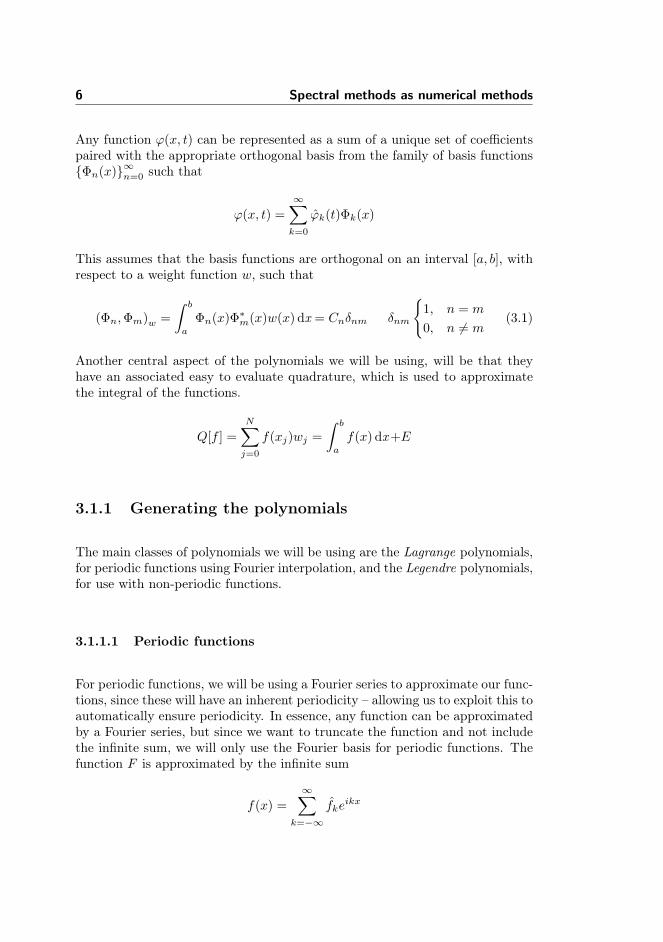
Figure 3.3: An illustration of Gibbs phenomenon by approximating a non-smooth function using only smooth functions. The approximationsare shown to the left, the coefficients are shown to the right.
Figure 3.3 shows that despite the increase in resolution, we maintain an error ofroughly the same size, it simply moves closer to the discontinuity. We also seethat the coefficients assume a close to constant value for rising n, which explainsthat the error will not decrease either.
3.1.3.2 Aliasing
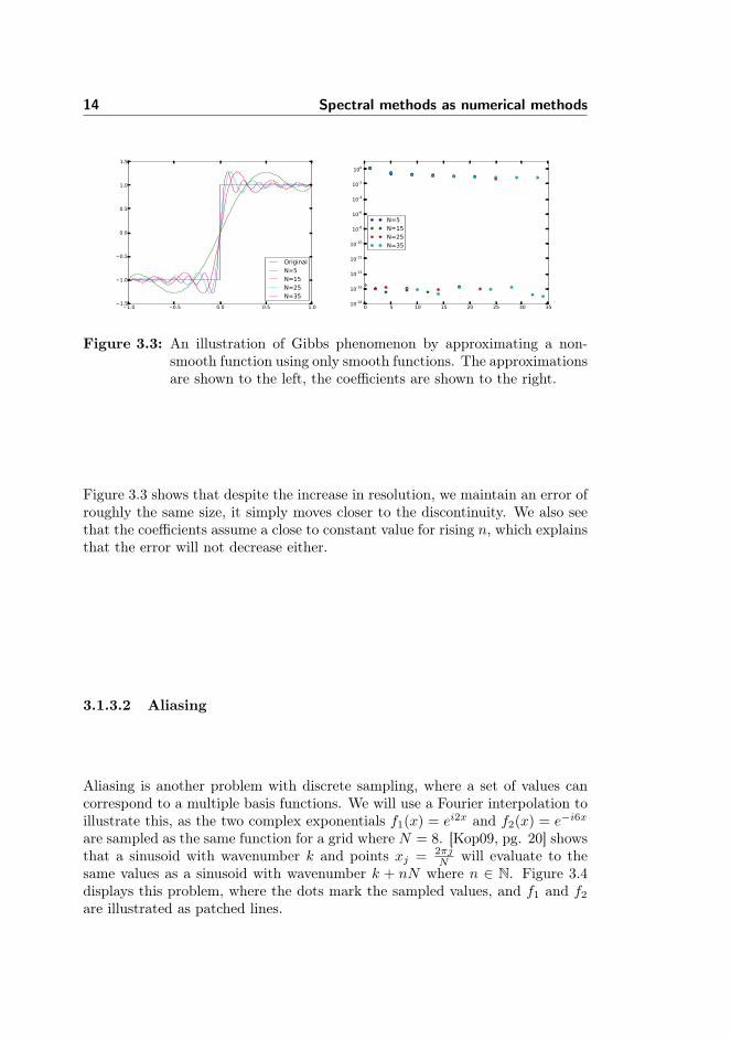
Aliasing is another problem with discrete sampling, where a set of values cancorrespond to a multiple basis functions. We will use a Fourier interpolation toillustrate this, as the two complex exponentials f1(x) = ei2x and f2(x) = e−i6x
are sampled as the same function for a grid where N = 8. [Kop09, pg. 20] showsthat a sinusoid with wavenumber k and points xj = 2πj
N will evaluate to thesame values as a sinusoid with wavenumber k + nN where n ∈ N. Figure 3.4displays this problem, where the dots mark the sampled values, and f1 and f2are illustrated as patched lines.

3.2 Constructing spectral solvers 15
0 1 2 3 4 5 6−1.0
−0.5
0.0
0.5
1.0k=2k=-6
Figure 3.4: On a grid with N = 8 points, the functions f1(x) = ei2x andf2(x) = e−i6x are illustrated.
3.2 Constructing spectral solvers
On the basis of the orthogonal polynomials, we will be constructing spectralsolvers for differential equations. We will be introducing two spectral methods,the collocation method and the Galerkin method. We will not be implementingthe Galerkin method, but briefly explain what it is, to indicate the differentways to implement spectral methods.
We will look at both the solution for boundary value problems, as well as thesolution for initial value problems.
3.2.1 Spectral methods
We will explain both the collocation method and the Galerkin method, andwhile the methods differ in how they approximate the solution as well as easeof implementation, they are both spectral methods, and can be used to achievespectral convergence for a differential problem.

16 Spectral methods as numerical methods
3.2.1.1 The collocation method
The collocation method is based on the idea of collocation points. The basic gistof this method is that we will aim to find an interpolating polynomial INf of afunction f , and we then want to enforce the relationship (3.7) at the collocationpoints.
INf(xj)− f(xj) = 0 (3.7)
This allows us to fulfill the differential equation at each of the collocation points,giving us N independent differential equations. Because of (3.7), we can com-pletely eliminate the need to convert coefficients for the actual implementation,since we will be using the nodal coefficients, which are identical to the functionvalues. This allows us to simple use the matrices derived in section 3.1.2 togenerate the values for the differentials in the differential equation.
The collocation method is very easy to implement, as we will show below, sinceit relies only on the differential matrices, which can be calculated beforehand– but it is also sensitive to aliasing errors, since it only concerns itself withthe solution at the collocation points. We have to implement the boundaryconditions as specific alterations to the operators, should we not be using theFourier collocation methods – where the boundaries are fulfilled by the basisfunctions.
For at problem defined as
ux + uy = 0
We simply construct a linear operator L = Dx + Dy, where the differential-operators are generated from the methods found in section 3.1.2, and we cansolve the problem by solving the linear equation
Lu = 0
3.2.1.2 The Galerkin method
The Galerkin method takes a different approach than the collocation method.We will seek a solution that fulfills the differential equation in basis space only,which means it will be using the weak form – fulfilling the differential equationonly as projected on the basis functions. For the problem
ux + uy = f(x)

3.2 Constructing spectral solvers 17
The Galerkin method will find the approximated solution v, which simply fulfills
(vx, φ) + (vy, φ) = (f(x), φ)
Where φ are the basis functions and (•1, •2) is the inner product, or projectionof •1 unto •2.
The orthogonality of the basis functions gives us N + 1 equations – one foreach basis function including n = 0 – and knowledge of the form the basisfunctions take will make us able to calculate an ordinary ODE for each of theN + 1 equations. This allows us to calculate directly using the modal coef-ficients, transforming into modal coefficients before we start calculations, andtransforming the coefficients to the solution after the calculations.
Since the Galerkin method operates in the modal basis, aliasing errors will not bea problem. The Galerkin method requires us to choose basis functions that fulfillthe boundary conditions, and calculating the the derivatives of these accordingto the differential equation. This makes it more cumbersome to implement ingeneral, since it will need to be tailored to each problem individually.
3.2.2 Types of differential equation problems
We have two main categories of partial differential equations, which we will besolving using our spectral methods, the initial value problems (IVPs) and theboundary value problems (BVPs).
3.2.2.1 Boundary Value Problems
Boundary values are a classic case of differential equations, specifically PDEs.They are characterized – as the name suggests – by supplying the values on theboundaries, and the differential equation then dictates how the interior of thesolution is related.
The primary method we will be using for these solutions, will be to create a lin-ear system of equations, where the solutions are the unknowns in the equation.We will be able to approximate the derivative of the function with the differ-ential operators, allowing us to isolate the function values in a linear system.The collocation approximation will generally lead to a dense system since theirdifferential operators are dense, while an application of the Galerkin methodmight yield a sparse system.

18 Spectral methods as numerical methods
3.2.2.2 Initial Value Problems
Initial value problems are another set of differential equation problems, where wewill be generating a solution from the initial value. This is typically time-relatedproblems, where we will be generating the time-derivative from the solution atthe prior time-step and its derivatives. We will be employing the same strategyas in the BVPs, where we will calculate the derivative values directly from thefunction values. This allows us to generate a set of time derivatives, which willbe used to solve a standard ODE problem.
Because the spectrum for the time-dimension is not exactly defined, we willnot be able to properly utilize the whole spectrum for our calculations, limitingour spectral methods to work on the remaining dimensions. This makes themethod used for solution a pseudo-spectral method, as it will be bounded bythe accuracy of the time-stepping integrator and not by the spectral accuracyof our methods. It will allow us to make N ordinary ODEs for time-stepping,which will be spectrally accurate in between time-steps.
3.3 Solving differential equations
We will employ the discussed methods on a selection of problems, where wewill solve a boundary-value problem and an initial-value problem in the form ofBurgers’ equation, which we will use for uncertainty quantification later as well.
3.3.1 Using the spectral collocation method
For this problem, we will be solving the differential equation
−ε d2
dx2u− d
dxu = 1 u(0) = u(1) = 0 (3.8)
Where ε = 0.01. The solution to this problem is found in Maple as
u(x) =e(1−x)/ε + e1/ε(x− 1)− x
1− e1/ε(3.9)
We will use a Legendre basis for this calculations, which means that we willbe using points defined from the Legendre-Gauss-Lobatto quadrature definedin (3.3). These nodes are defined for xGL ∈ [−1, 1], and we will need to scale
3.3 Solving differential equations 19
them to our domain, which is x ∈ [0, 1], which means that we will apply thetransformation
x =xGL + 1
2⇔ xGL = 2x− 1
This transformation gives us a scaling factor, which we can calculate as
dxGLdx
= 2
Using the spectral collocation method, defined in (3.7), we will seek to satisfythe solution uN the following problem
−εd2uNdx2
(xi)−duNdx
(xi) = 1 1 ≤ i ≤ N − 1uN (xi) = 0 i = 0, N
Using the differential operator from section 3.1.2.2, we can approximate duN (x)dx =
2D · u and d2uN (x)dx2 = 4D2 · u. This allows us to write the problem as
−ε4D2x− 2Dx = 1⇔(−εD2 −D
)x = 1
By creating the linear operator L = −ε4D2−2D, we can impose boundary con-ditions simply by modifying the first and last rows of L such that it correspondsto 1 ·x0 + 0 ·xn = 0 and 1 ·xN + 0 ·xm = 0 where n ∈ [1, N ] and m ∈ [0, N − 1].The right-hand-side vector b needs to be changed as well, such that bi = 1 for1 ≤ i ≤ N − 1 and bi = 0 otherwise.
This allows us to solve the problem defined in (3.8) spectrally by solving thelinear system Lu = 1. The implementation of this problem will be handled insection 4.4.1.
3.3.2 Burgers’ equation
The viscous Burgers’ equation is a partial differential equation of the form
ut + uux = vuxx x ∈ [−1, 1] (3.10)u(−1, t) = 1 u(1, t) = −1 ,∀t > 0
v > 0
This equation will assume a steady state after t has become high enough, as-suming it has an initial condition that satisfies the boundaries. We will be usingthe function −tanh(x) 1
|−tanh(−1)| , which will be normalized for the endpoints to1 and −1.
20 Spectral methods as numerical methods
In order to derive the time-step, we will be using the collocation method as de-scribed in section 3.3.1 to approximate the solution, which gives us the solutionapproximated with the Legendre-Gauss-Lobatto nodes xi
duNdt
(xi, t) + uN (xi, t)duNdx
(xi, t) = vd2uNdx2
(xi, t) 1 ≤ i ≤ N − 1
u(x0, t) = 1 u(xN , t) = −1
Since we are using the collocation points xi, we can generate the differentialoperator D from section 3.1.2.2 and approximate the differentials, giving us.
duN(t)
dt+ uN(t)(DuN(t)) = v
(D2 · uN(t)
)⇔
duN(t)
dt= v(D2 · uN(t)
)− uN(t)(DuN(t)) (3.11)
Since we have an established initial condition, we will simply need to ensure thatdu(0)
dt = 0 and du(N)
dt = 0, and we can solve this as a coupled ordinary differentialequation, using this pseudo-spectral method.
The implementation of Burgers’ equation will be handled in section 4.4.2.
Chapter 4Implementation of spectral
methods
The implementation of the methods is critical to the methods. If the imple-mentation is wrong, we will not be able to achieve the spectral convergencewe desire. It is important that the method of implementation is chosen wisely,such that it will be able to support the computations accurately. We will beusing [Big12] for many of the polynomial computations we will be doing, as thispackage includes functions to evaluate most polynomials apart from the Fourier.
Python has been chosen as the programming language due to the portabilitycompared to the licensed MATLAB – Python can run on most platforms, and itis free to download and install. Python also supports a wide array of librariesthat mimic the functionality of MATLAB, allowing us to use Python with relativeease.
4.1 How to use Python for numerical computa-tions
Using Python as a programming language is not that different from using MATLAB– the code is easy to read, write and understand. Python is unlike a lot of other
22 Implementation of spectral methods
programming languages in that it does not use parentheses to indicate nestingof functions or conditions, but rather uses indentation – as most other languagesuse only as a standard. This gives Python code a guarantee that it will be easyto read, as the standardization of the code formulation is inherent in the way itworks.
Python is – just like MATLAB – a high-level interpreted programming language,allowing the user to focus on the coding aspects of the code, and leave handlingmemory-management, variable types and other machine-dependent things tothe Python interpreter. This also gives it the quality for effective debugging, asyou literally step your way through the code, seeing the results as you go, whichcan be invaluable when trying to discover a calculation error in an implementedmethod.
In addition to this, Python is non-commercial and cross platform, allowingPython scripts to be run on any machine without a license. This, and thefact that it is designed as a general purpose language, allows for a very versatileimplementation, that can be improved and run anywhere, by anyone. WhereMATLAB requires a commercial license to use or even run already compiled code,Python is free. Python also allows for easy interfacing with most other lan-guages, specifically C and C++, further broadening the spectrum of use withPython.
4.1.1 A comparison to MATLAB
Most MATLAB code can be almost cleanly translated to Python code, thanks tothe Python packages NumPy, SciPy and Matplotlib. There are however someclear differences that must be accounted for.
• Zero index – Python uses a zero-indexing standard, while MATLAB usesa one-indexing standard, making most algorithms give a one-off error ifdirectly converted. This is quickly fixed though, but requires some applica-tion of thought for algorithms where the index is part of the mathematicalcalculations.
• Basic array actions – Python is designed as a general purpose languageand does not automatically assume that we are working in matrices. Thisgives most common operators an element-wise property, with specializedfunctions for matrix products and other matrix operations. While Pythoncontains classes for simulating the matrix class in MATLAB, it is not broadlyemployed as it is limited to 2-dimensional matrices.
4.1 How to use Python for numerical computations 23
• Differencing between arrays and functions – Python does not al-low accessing arrays by the a(1) standard and instead uses a[1]. Thiscan cause some confusion as to why a function will not run but can bequickly eliminated, as it casts an error. Functions are still called with softparentheses.
• Implementing sub-functions – Unlike MATLAB, a Python file can containseveral sub-functions that can be accessed from another file, and it is notrestricted to the same name as the function either. This allows for acleaner code-hierarchy.
• Slicing arrays – A Python slice of an array is issued with the : operatorlike MATLAB, but unlike MATLAB, beginning and end are assumed unlessstated otherwise. This allows the formulation a[3:] if you want thearray from the fourth element onwards. For accessing the elements in thelast part of an array, negative numbers are used, and a[-1] will net thelast value of an array. Unlike MATLAB, slice operations do not copy thearray, but simply provides a view into it. This can cause problems withiterative algorithm that assumes the array is constant – Python uses thecopy function to copy arrays, where MATLAB copies them as default.
4.1.2 Employed Python packages
Python allows for a vast number of different capabilities, with a wide-rangingpackage-portfolio. We will concentrate on the five packages that we will be usingfor our spectral methods and uncertainty quantification.
4.1.2.1 NumPy — Numeric calculations in Python
NumPy is a function library that supports large multi-dimensional arrays, aswell as including modified versions of standard mathematical functions, so theycan be employed upon these large arrays. It draws heavy inspiration fromMATLAB, with most of the functions being called the exact same thing as inMATLAB, like linspace and ones. It also supplies functions for matrix multipli-cation and linear solving through the linalg module. It will most commonly beimported simply as np in this code, allowing calling of functions by np.linspace.
A complete description and list of features can be found on http://docs.scipy.org/doc/numpy/contents.html
24 Implementation of spectral methods
4.1.2.2 SciPy — Scientific methods for Python
SciPy is a function library that employs a lot of scientific functions, such as fastFourier transform, ODE integrators, data input and output, statistical functionsand much more. It is intimately tied to NumPy, as many of these functions usethe NumPy array as standard input and output type.
A complete list of features and can be found on http://docs.scipy.org/doc/scipy/reference/
4.1.2.3 Spyder — A MATLAB imitating development environment
Spyder imitates the development environment provided in MATLAB, to a lot offeatures. It supplies easy step-by-step debugging, variable editing while running,and multiple Python consoles. The layout is easily recognizable as the MATLABinterface, and even supports an automatic object inspector, which provides thehelp documentation for any functions imported properly.
The homepage of the Spyder development interface is found at http://code.google.com/p/spyderlib/
4.1.2.4 Matplotlib — The Python plotting tool
Matplotlib supplies many visualization options to Python, but most notable isthe pyplotmodule, which mimics MATLABs plotting features. The pyplot modulecontains functions nearly impersonating MATLAB functions, where the names ofthe functions are called the same as in MATLAB, allowing for very easy conversionbetween these two development interfaces. It only supports 2D plotting, needingsupport in order to achieve 3D plotting, and is also limited by the fact that aplot needs to be closed before data can be manipulated again. These are minorannoyances, and we will be using this library to visualize most of our functions.We will mostly be importing this library as plt, allowing us to plot with thecommand plt.plot(x,y)
Matplotlib is a comprehensive library, with all the documentation found athttp://matplotlib.org/
4.2 Challenges using Python instead of MATLAB 25
4.1.2.5 DABISpectral1D
DABISpectral1D is a module developed by Daniele Bigoni, PhD student at DTUCompute. It is used for generating the needed values for orthogonal polynomialsused in spectral methods. We will be using this to calculate most transforma-tions and quadratures with the Legendre polynomials as well as the Hermitepolynomials needed later. It works by first initializing a polynomial as a vari-able, and this polynomial will then contain the functions needed for quadraturesand transformations as sub-functions. We will typically be importing it as DB,allowing us to call functions as DB.Poly1D()
4.2 Challenges using Python instead of MATLAB
Using Python instead of MATLAB does prove somewhat difficult regarding somepitfalls one may encounter. We will document here how they might affect theprocess, and how to overcome them.
4.2.1 Integer division
Python is not used exclusively as a numeric language, and because of this it doesnot automatically cast integer division as a floating point number, should thedivision not have an integer solution. Python automatically casts integer divisionto another integer, rounding the result down. This can prove problematic ifany of the mathematical expressions include a fraction like 1
2 . It can be easilyovercome though, with two easy solutions.
• Adding a punctuation mark after the integer, to indicate it should betreated as a floating point value. In the above example we would thenwrite 1./2. instead of 1/2.
• Importing the built-in function to convert integer division to floating pointnumbers automatically. This will require the very first line of code in therelevant file to be "from __future__ import division".
Both of these fixes are very easy to implement, although it can easily ruin acode if not remembered, as it will not throw any error, despite reducing theproduct it is a part of to zero. We will mainly be employing the second methodto ensure that we will not have any fractions we have forgotten.

26 Implementation of spectral methods
4.2.2 Interfacing with MATLAB
One of the biggest challenges is interfacing with the many MATLAB scripts whichare available. Many results are approximated using MATLAB scripts, which willbe useful for verifying implementations. There are a few ways that we can solvethis problem
• Convert the scripts – If we convert the scripts manually, they will runnatively with Python. This is fairly straightforward for smaller programs,but can be a daunting task for longer scripts. For most longer scriptswe would have to keep track of which variables are matrices/vectors andwhich are simply constants, in order to update the script correctly, aswell as finding Python replacements for build-in functions that are notstandard.
• Saving the data – MATLAB can save the data as a .mat file, which is fairlyeasy data-format to read, which SciPy can easily read. It requires thatthe problem can be replicated exactly in order to compare with the data,something which is not always possible.
• Actual interface – Many Python libraries exist that can directly interfacewith MATLAB. This requires the running computer to also have a MATLABinstallation, which eliminates the absolute portability of the scripts. Thiscan easily be used for verification purposes, and be disabled in the fi-nal scripts, allowing seasoned MATLAB coders to test their Python scriptsagainst old experiences before shipping Python code.
We will not be dependent on MATLAB scripts that are big enough to not beconverted properly. Most of the data we will be using for confirmation is alsoof the size to simply write into our files. This means that we will at no time beusing the options of loading MATLAB data or interfacing with MATLAB.
4.2.3 Python overhead
Python is a general purpose programming language, and is thus not optimizedto do the advanced mathematical computations, as MATLAB is. While Pythonhas many features, they come with the price of an overhead time-cost MATLABdoes not have. Unlike MATLAB, effort must be made if Python has to become aseffective as MATLAB, but it is unlikely that it is possible, due to the de-centralizeddevelopment of Python. While this overhead in general is not pronounced, itbecomes quite pronounced when dealing with big systems as the ones we will

4.3 Implementation for spectral methods 27
handle in chapter 6. While this is unfortunate for aspiring numerical users ofPython, it is not crippling to the process. This issue is magnified the moredifferent packages are used for the calculations, so it is always a good idea toonly import the packages you need and use when doing numerical computationsin Python.
4.3 Implementation for spectral methods
Before we will be able to solve our problems with spectral methods, we willneed to construct some of the parts that we will be using for our spectral solvers.These implementations or scripts will be used in the development of our spectralmethods.
4.3.1 Generating the differential operators
The differential operators will be central to the collocation method, as these willfind the numerical differentials of the nodal values by a simple matrix product.We will split this into the definition of the Lagrange Fourier matrix DF andthe Legendre matrix DP, which will both be included in a Python script calledDiff.py, from where we will import them when needed. We will not be utilizingthe Fourier differential operator, but implementing it is necessary to be able tohandle periodic boundaries in problems.
4.3.1.1 The Fourier differential operator
We recall the definition of the Fourier differential operator from (3.5), and notethat it is only defined for a grid of even points. Using this, we will implement

28 Implementation of spectral methods
the matrix by the following algorithm.
Data: N - Positive integer designating the size of the array containing theequally spaced points.
Result: A Fourier differentiation matrix DD = Zero NxN Matrixfor i← 0 to N − 1 do
for j ← 0 to N − 1 doif j 6= k then
D[i][j] = 12 (−1)
1+k+jcot(π(j−k)N
)else
D[i][j] = 0end
endend
Algorithm 1: Generating the Fourier differential matrix
The reason that we are excluding the last point, is that it is automaticallyassumed that the last point be equal to the first one by periodicity. The codefor this implementation can be found in appendix D.1.
We will test this implementation by creating a function v(x) = esinπx definedon the grid x ∈ [0, 2]. This will have the true solution v′(x) = π cos (πx)esinπx,which we will be able to test up against. Using algorithm 1, we will calculatethe derivatives, and the convergence with regards to the number of points N
0.0 0.5 1.0 1.5 2.0x
−6
−4
−2
0
2
4
6
v'(x)
AnalyticApproximation
100 101 102
N
10-14
10-13
10-12
10-11
10-10
10-9
10-8
10-7
10-6
10-5
10-4
10-3
10-2
10-1
100
ErrorN^(-3)
Figure 4.1: The numeric differential (by Fourier operator) of v(x) to the left,and the convergence to the right.
Figure 4.1 shows that the differentials are quite precise at even relatively small

4.3 Implementation for spectral methods 29
numbers of N , and that the error converges faster than polynomial speed, satis-fying the condition to be used in a spectral solver by having spectral accuracy.
4.3.1.2 The Legendre differential operator
The definition for the differential operator we will need for non-periodic func-tions is explained in section 3.1.2.2. Since we know that the differential operatoris calculated as
D = VxV−1
Where V is the Vandermonde matrix, and Vx is the Vandermonde matrix of thedifferentiated basis polynomials, when we have calculated them, we will be ableto construct the differential matrix. The package DABISpectral1D contains aroutine to compute the Vandermonde matrix of derivative order n on a set ofpoints x, which we will be using. This allows us to generate the differentialoperator as
Data: N - Positive integer designating the size of the array containingLegendre-Gauss-Lobatto quadrature points.
Result: A Legendre differentiation matrix DD = Zero NxN MatrixCreate the Legendre-Gauss-Lobatto nodes xGL from N withGaussLobattoQuadrature from DABISpectral1DCreate V from N and xGL with GradVandermonde from DABISpectral1DCreate Vx from N and xGL with GradVandermonde from DABISpectral1DSolve the system VD = Vx for D with numpy.linalg.solve
Algorithm 2: Generating the Fourier differential matrix
This implementation can be found in appendix D.1.
We will test the algorithm 2 implementation on the same function as the testfor algorithm 1.

30 Implementation of spectral methods
0.0 0.5 1.0 1.5 2.0x
−6
−4
−2
0
2
4
6
v'(x)
AnalyticApproximation
100 101 102
N
10-11
10-10
10-9
10-8
10-7
10-6
10-5
10-4
10-3
10-2
10-1
100
101
ErrorN^(-2)
Figure 4.2: The numeric differential (by Legendre operator) of v(x) to the left,and the convergence to the right.
As we can see in figure 4.2 the nodal points are not located with the same equalspacing as in figure 4.1. The nodal values are centered more towards the ends ofthe spectrum. We also see that the Legendre differential operator also achievesspectral convergence, qualifying it for use with spectral methods.
4.3.2 Employing the time-stepping method
For the time-dependent problems, we will need an established time-stepping al-gorithm in order to get dependable results. For this we will use the functionscipy.integrate.odeint in most cases. This method is based on the LSODAalgorithm from the FORTRAN ordinary differential equation solver pack, ODEPACK.It automatically adjusts the time-steps, adjusting to the problem stiffness, mak-ing it a good choice for us, since we will not have to calculate a stable solver foreach problem.
The function is called as odeint(func, y0, t, (args)), where the inputs are
func A right-hand-side function which returns the time-derivatives
y0 A vector of the initial states
t A vector containing the time-values we would like to have output thefunction values for. The first element should be the initial time, and thelast should be the last time.
args A Python tuple, containing all the extra arguments to pass to func.

4.3 Implementation for spectral methods 31
The function then returns a RNy×Nt matrix, where each column represents atime-step.
Using this function will force us to define the right-hand-side function explicitly,and ordering all our values into a single vector. This will force us to gather allinput values into a vector before using this, and including a splitting procedurein func. With this in mind, we can employ this as part of the solution for initialvalue problems.
An example of such a right hand side function can be found in the implemen-tation of Burgers’ equation from section 4.4.2.
def dudt(u,t,v,Dx,BoundaryFixer):#Calculate the linear operator
unew= -u*np.dot(Dx,u)+v*np.dot(Dx,np.dot(Dx,u))
#Adjust for boundariesunew = unew*BoundaryFixerreturn unew
4.3.3 Handling multi-dimensional problems
One problem that will arise will be how to handle multi-dimensional problems.The problem with multi-dimensional problems, is that not only will the problemlikely need to be passed as a vector for some functions, but our differentialoperators are also only defined in the 1D spectrum.
4.3.3.1 Multiple dimensions in a single vector
To define a grid of values, we will use a vector of values along each dimension, xand y, and we will create the needed grid by the command X,Y=numpy.meshgrid(x,y),which will net us the grids
X =
x0 x1 · · · xNx
x0. . .
......
. . .x0 · · · · · · xNx
Y =
y0 x0 · · · y0
y1. . .
......
. . .yNy · · · · · · yNy

32 Implementation of spectral methods
We will need to be able to order an entire multi-dimensional array into onevector for the time-integration scheme we have developed. We will do this byutilizing some of the built-in functions of Python, flatten and reshape.
In order to vectorize our multi-dimensional array, we will use the build inflatten function, where we will specify we want to flatten it using the for-tran standard, which is column-major – the first column will be the first partof the new vector, followed by the second column and so on (same result as theMATLAB notation a(:)). Now, we can reform the vector to its previous stateusing reshape, where we will need to specify the number of elements in eachdimension, and the order with which we flattened it.
To avoid continuously flattening and reshaping, we will create a multi-dimensionalarray of indexes, which will include the index of each point in the vector, locatedat the point it should be in the matrix. We will accomplish this by creating anarray of indexes, and reshaping this as we would have our vector. This allowsus to use the notation A[index[x,y]] instead of reshaping A to use A[x,y].
An example for the functions mentioned used in included below
x,wx = LegPol.GaussLobattoQuadrature(Nx)y,wy = LegPol.GaussLobattoQuadrature(Ny)
X,Y = np.meshgrid(x,y)
u = u.flatten("F")
index = np.arange((Nx+1)*(Ny+1)).reshape(Ny+1,Nx+1,order=’F’).copy()
4.3.3.2 Differentiation of multiple dimensional array
Since our differential operators are only defined on the single dimensional space,we will need to find a way to differentiate the multi-dimensional arrays as ifthey were in a single dimension. We will use the vectorized version of the multi-dimensional array. If we recall that the first column would be ordered at thetop, followed by the next column. If we individually used the differentiationoperator on each column, we could differentiate those values along the first axis.To do this, we can generate a new matrix DX 6= Dx, which would be definedas DX = Dx ⊗ INy , where INy is the identity matrix of size Ny × Ny, and ⊗is the kronecker product. This would allow us to use the dot product betweenDX and our vector of values v to generate dv
dx = DX · v. Using the same logic,
4.3 Implementation for spectral methods 33
we can differentiate along the other axis using DY = Dy ⊗ INx . For N > 2dimensional problems, we would add a kronecker product for each dimension.
In order to verify this, we create a mesh from x ∈ [−1, 1] and y ∈ [−1, 1], wherewe will generate the function cos (xy) over. Differentiating this along both axiswill give
d
dx
d
dycos (xy) = −xy cos (xy)− sin (xy)
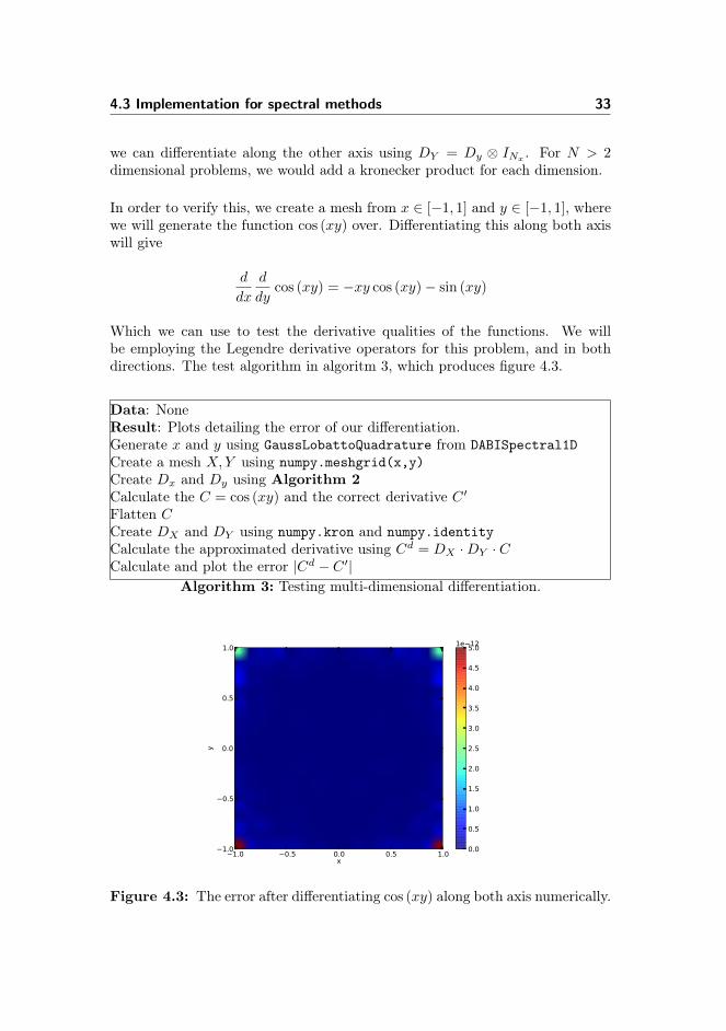
Which we can use to test the derivative qualities of the functions. We willbe employing the Legendre derivative operators for this problem, and in bothdirections. The test algorithm in algoritm 3, which produces figure 4.3.
Data: NoneResult: Plots detailing the error of our differentiation.Generate x and y using GaussLobattoQuadrature from DABISpectral1DCreate a mesh X,Y using numpy.meshgrid(x,y)Create Dx and Dy using Algorithm 2Calculate the C = cos (xy) and the correct derivative C ′Flatten CCreate DX and DY using numpy.kron and numpy.identityCalculate the approximated derivative using Cd = DX ·DY · CCalculate and plot the error |Cd − C ′|
Algorithm 3: Testing multi-dimensional differentiation.
−1.0 −0.5 0.0 0.5 1.0x
−1.0
−0.5
0.0
0.5
1.0
y
0.0
0.5
1.0
1.5
2.0
2.5
3.0
3.5
4.0
4.5
5.01e−12
Figure 4.3: The error after differentiating cos (xy) along both axis numerically.

34 Implementation of spectral methods
As figure 4.3 shows, the error is in the order of machine accuracy, showing thatthis differentiation scheme works as intended.
The full code for the test can be found in appendix D.2.
4.3.4 Sparse matrices
The multi-dimensional differential-operator matrices – as a kronecker productwith the identity matrix – consist largely of zeroes. NumPy does not nativelysupport sparse matrices, but SciPy includes a library that supports sparse ma-trices. This means that we will need to monitor which of our matrices are sparse,and modify the expressions where they are a part.
Since we will mainly be using this on the differential operators – from which allwe need is the dot product – we can utilize the inherent function of the sparsematrices A.dot(b) to get the dot product A · b in a standard vector format.
SciPy offers many different formats for sparse matrices, each suited for differentapplication, and we will be using a form classified as compact-sparse-row matrix,as this will be most efficient for the dot-product according to [JOP+ ].
In order to verify that this is indeed faster, and as correct, we will constructa test-case for this sparse matrix, where we will generate a random 1000x1000matrix A, with non-zero elements in 100 places in the first two rows, and nonzeroelements along the diagonal, and generate a random nonzero 1000x1 array b.We time both the sparse version of the dot product and the full version, andrepeat this procedure 1000 times. This gives us an average of 2.778 · 10−3
seconds for the full dot product, and only 1.289 ·10−4 seconds in average for thesparse dot product, giving us a significant upgrade in speed. The average error‖x2sparse − x2full‖2 was 5.4 · 10−13, which is within acceptable bounds, as we canattribute that to machine accuracy.
The full code for this test can be found in appendix D.2.
4.4 Practical implementation
We have outlined how to implement the different parts of the code, and now wewill implement the actual solutions to the problems from section 3.3, in orderto verify the implementation works, and the convergence behaves as expected.

4.4 Practical implementation 35
4.4.1 Implementing the spectral collocation method
We will use the problem from section 3.3.1, which is defined as
−ε d2
dx2u− d
dxu = 1 u(0) = u(1) = 0
And has the solution (3.9).
Since the derivation was handled in the previous chapter, we will simply imple-ment the method here, using the routines described in this chapter. We choosethe Legendre polynomials to model the equations, which means that we will gen-erate the differential matrices using algorithm 2. Since this algorithm alreadyuses the untransformed points, we will use these as well for our problem.
The construction and modification of our linear operator to adhere to boundarypoints is done as follows
#Construct LL = -epsilon*4*np.dot(D,D) + b*2*D
#Implement boundary conditionsL[0,:] = 0L[-1,:] = 0L[0,0] = 1L[-1,-1] = 1
#Generate right-side function with boundary conditionsf = np.ones((n,1))f[0] = 0f[-1] = 0
After having constructed our linear operator, we will use the function solvefrom the numpy.linalg pack to find the solution. We will continuously increasethe amount of points between 10 ≤ N ≤ 80 in order to generate an errorconvergence plot.

36 Implementation of spectral methods
0.0 0.2 0.4 0.6 0.8 1.0x
0.0
0.2
0.4
0.6
0.8
1.0N=80 and epsilon=0.01
ApproximationExact
101 102
N
10-15
10-14
10-13
10-12
10-11
10-10
10-9
10-8
10-7
10-6
10-5
10-4
10-3
10-2
10-1
100
Error \epsilon=0.01
Figure 4.4: To the left: The calculated solution using N = 80 to the problemgiven in (3.8), compared to the correct solution as given in (3.9).To the right: The error for the approximation as a function of N
Figure 4.4 shows us that the solution is indeed spectral in convergence, andthat the spectral collocation method can be implemented with the previouslydescribed methods.
The full code for the test case can be found in appendix D.3.
4.4.2 Burgers’ equation – implementing the solver
We will be implementing the solution we found in section 3.3.2, which is theviscous Burgers’ equation described as
ut + uux = vuxx x ∈ [−1, 1]
u(−1, t) = 1 u(1, t) = −1 ,∀t > 0
Since the problem has Dirichlet boundary conditions, we will be using the Leg-endre polynomials to, and thus the differential operator from algorithm 2. Usingthe derived form from (3.11), we construct a separate right-hand-side function,in which we include the condition that the time-derivative will be zero on theboundaries.
The right hand side and the "boundary fixer" are constructed as such
#Create boundary fixer to cancel the time derivatives# at the boundaries.

4.4 Practical implementation 37
BDFix = np.ones(x.shape)BDFix[0] = 0BDFix[-1] = 0
def dudt(u,t,v,Dx,BoundaryFixer):#Calculating linear operatorunew= -u*np.dot(Dx,u)+v*np.dot(Dx,np.dot(Dx,u))#Adjust for boundariesunew = unew*BoundaryFixerreturn unew
By multiplying the time-derivative with BDFix, all values will remain the same,except at the boundaries, where the boundary values time-derivative is equal tozero.
We use the time-stepping function described in section 4.3.2, where we generatethe initial condition from the function u0(x) = −tanh(x) 1
|−tanh(x0)| .
In order to generate a numerical solution, we will need to define v > 0, whichwe choose to be v = 0.1.
−1.0 −0.5 0.0 0.5 1.0x
−1.0
−0.5
0.0
0.5
1.0
Solution to Burgers' equation
Initial Valuet=0.40t=0.80t=1.20t=1.60t=2.00t= 4
Figure 4.5: The solution to Burgers’ viscous equation with v = 0.1.
We see in figure 4.5 that the equation quickly achieves a steady state.
The full code for the test case can be found in appendix D.3.

38 Implementation of spectral methods
Chapter 5
Stochastic formulation anduncertainty quantification
The influence of measuring errors or other uncertain quantities in a differentialequation can sometimes change the solution drastically. To enable us to tocorrectly gauge the effect of uncertainties, this chapter describes how to quantifyand implement these factors into our differential equation models.
This will an effective aid in assessing the impact uncertainty can have on com-plicated systems where it can often be very hard or impossible to predict. Wewill mainly be using the method called generalized polynomial chaos, which al-lows us to drastically reduce the time needed to do calculations with acceptableerrors – making the effort worthwhile even under a certain time-constraint.
5.1 Probability theory
In this section, we will explore the probability theory needed to utilize andunderstand uncertainty quantification. We will start by introducing the basicconcepts for probability and stochastic computations, and move on to how wewill formulate and solve stochastic problems numerically. We will draw heavilyon [Xiu10, Chp. 2], which presents and defines these concepts.

40 Stochastic formulation and uncertainty quantification
5.1.1 Basic concepts
In order to include stochastic variables in our models, we need to classify theseand the concepts associated with them.
5.1.1.1 Random variables
The concept of random variables is essential to the formulation of our problems.A random variable is, in essence, what allows us to represent the random natureof our system. We assign a possible outcome the designation ω, wether it be aphysical outcome, such as heads or tails in a coin-flip, or a numerical outcome.This allows us to create the random variable concept as a real-valued functiondependent on ω, such as the random variable X = X(ω). The random variablecan now always be represented in a mathematical model, despite the outcomesnot always being mathematical in nature.
This allows us to represent information about a given mechanic, where we candefine how the outcome might work, but might not be sure how the exactmechanics work.
The random variables in this thesis will have outcomes already defined on thenumerical scale, and but will retain the notation X(ω) as it is still a function ofthe random outcome.
5.1.1.2 Distributions
Random variables are all associated with a given probability, which measuresthe likelihood that each outcome will be the realization of ω. The probabilityof each outcome is a number 0 ≤ p ≤ 1, where 1 signifies that the outcomealways happens, and 0 that it never happens. Associated with the probabilityis the distribution function FX , which is the accumulated probabilities FX(x) =P (X ≤ x).
The distribution is often used to characterize the variable for continuous distri-butions, which are a large part of what we will be working with. Most continuousdistributions also have a density fX which is used to characterize the probabilityfor a given range of outcomes. Since the distribution is continuous it followsthat there is exactly P (X = x) = 0 chance for a given outcome to occur. We
5.1 Probability theory 41
therefore define the density as
FX(x) =
∫ x
−∞fX(y) dy
Where fX(x) ≥ 0 and the sum of all outcomes is exactly 1,∫∞−∞ fX(y) dy = 1.
The two distributions we will be working with will be the gaussian distributionand the uniform distribution. The density of the gaussian distribution N
(µ, σ2
)where x ∈ R is defined as
fX(x) =1√
2πσ2e−
(x−µ)2
2σ2 (5.1)
And the uniform distribution U(a, b) is constant for x ∈ [a, b]
fX(x) =
1b−a x ∈ [a, b]
0 otherwise
5.1.1.3 Moments and expectation
Moments are a very useful way of describing a random variable X, since we cancharacterize the behavior of a random variables using a few concepts. The mthmoment is defined as
E[Xm] =
∫ ∞−∞
xmfX(x) dx
The most commonly used moment is probably the first moment, which is alsocalled the expectation or the mean value. This characterizes the most likelyvalue to be assumed by the variable, hence the name expectation. It is typicallydenoted as µ, and is used as this to characterize the gaussian distribution, asseen in (5.1).
With the expectation defined, we can define another widely-used concept derivedfrom moments, which are the centered moments. They are defined as
E[(X − µX)m
] =
∫ ∞−∞
(x− µX)mfX(x) dx
The first centered moment will always evaluate to zero. The second centeredmoment is called the variance, denoted σ2, and is the square of the standarddeviation σ. The standard deviation is used to describe how far the variation

42 Stochastic formulation and uncertainty quantification
is around the mean, for example 95% of values are within µ ± 2σ for a gaus-sian distribution. It is worth noting that a gaussian distribution is completelycharacterized by the mean and standard deviation.
We will operate with functions of random variables rather than random variablesthemselves. Many of the concepts can be directly applied to functions as well,although the mathematical calculation differs a bit. For any real valued functiong the expectation is calculated by
E[g(X)] =
∫ ∞−∞
g(x)fX(x) dx
5.1.2 How to formulate a stochastic problem
To investigate the effects of having stochastic variables in the formulation of oursystem, we will need to formulate the problems differently. Given a differentialsystem with stochastic variables, we will need to identify and parameterize thestochastic inputs, allowing us to do computations based on these.
Parametrization is generally uncomplicated if the stochastic variables are al-ready operating in RN , and are independent. Since this thesis is generallyconcerned with already parameterized domains, we can typically model ourstochastic variables to this domain – making further parameterization unneces-sary.
5.1.2.1 Generalized polynomial chaos
Generalized polynomial chaos (gPC) is a technique used for parametrization ofa stochastic variable. It involves modeling a stochastic variable by an appro-priately chosen polynomial, allowing easing of the calculations for expectations.By modeling the stochastic variables as a polynomial, we can choose the valuesof our stochastic variables with a deterministic routine instead of allowing thesevalues to be "random".
In general the basis functions of gPC are the polynomials satisfying
E[Φm(Z)Φn(Z)] = γnδmn m,n ∈ N (5.2)
It is clear from the delta-function, that these polynomials must be orthogonal,and that
γn = E[Φ2n(Z)
]n ∈ N

5.1 Probability theory 43
For the probability density function ρ(z), we can calculate the expectation from
E[Φm(Z)Φn(Z)] =
∫Φm(z)Φn(z)ρ(z) dz = γnδmn (5.3)
[Xiu10, Table 5.1] suggest that for gaussian distributions, Hermite polynomialsare chosen for the basis, and for uniform distributions Legendre polynomials arechosen.
Hermite polynomials Hermite polynomials are a family of orthogonal poly-nomials defined as
Hn(x) = (−1)nex
2/2 dn
dxne−x
2/2
And satisfying∫ ∞−∞
Hm(x)Hn(x)w(x) dx = n!δmn w(x) =1√2πe−x
2/2 (5.4)
The similarity between the weight function and the actual density for a gaus-sian variable suggests that Hermite polynomials are easy to use when modelinggaussian variables. The density of gaussian variables is
fX(x) =1√
2πσ2e−
(x−µ)2
2σ2 (5.5)
Which means that the Hermite weight function is exactly the density of thegaussian variable X N (0, 1). The first six Hermite polynomials are visualizedin figure 5.1
−3 −2 −1 0 1 2 3−30
−20
−10
0
10
20
30
HP0HP1HP2HP3HP4HP5
Figure 5.1: The first six Hermite polynomials visualized
44 Stochastic formulation and uncertainty quantification
5.1.3 Calculating the expectation
The expectation of a stochastic variable X is defined as
E[X] =
∫ ∞−∞
xfX(x) dx
For our calculations, we will not always have the analytic solution to the dis-tribution of our values we will not be able to use this integral, but rather aquadrature. For a set of N points chosen at random, we will assign each pointthe same weight, giving us
E[X] =
N∑n=0
1
Nxn for large N
This is a a result of the law of large numbers, which states that
limN→∞
N∑n=0
1
Nxn = µx
5.1.3.1 Gaussian distribution
For a gaussian distribution, we use the Hermite polynomials to approximate thevariable, we will instead use the Gauss-Hermite quadrature, which is defined as∫ ∞
−∞f(x)e−
x2
2 dx ≈n∑i=1
wif(xi) (5.6)
If we want to calculate the expectation of the modeled variable, we use thedefinition from section 5.1.1.3
E[g(X)] =
∫ ∞−∞
g(x)fX(x) dx
Since we will only be modeling gaussian variables by Hermite polynomials, wecan calculate these expectations as
E[H(X)] =
∫ ∞−∞
1
σ√
2πH(x)e−
(x−µ)2
2σ2 dx
Since we would like to use (5.6), we will need to employ a transformation to
x→ y, such that e−(x−µ)2
2σ2 = e−y2
2
y =x− µσ⇔ x = σy + µ
5.2 Quantification of uncertainty 45
This would allow us to calculate the expectation by (5.6)
E[H(X)] =
∫ ∞−∞
1√πH(σy + µ)e−
y2
2 dx ≈ 1√π
n∑i=1
wiHi(σyi + µ) (5.7)
5.1.3.2 Uniform distribution
If we want to use the uniform distribution instead of the gaussian, we will beusing the Legendre-Gauss quadrature instead. We assume a random variable Yis following the uniform distribtion Y ∼ U(a, b)
E[L(Y )] =
∫ b
a
L(y)fY (y) dy =
∫ b
a
L(y)1
b− ady
Since the Legendre-Gauss quadrature only works on the interval [−1, 1], so wetransform y
x =b− a
2y +
a+ b
2
dx
dy=b− a
2
This allows us to calculate the expectancy by the Legendre-Gauss quadrature
E[L(Y )] =b− a
2
∫ 1
−1L(x)
1
b− adx =
1
2
∫ 1
−1L(x)⇔
E[L(Y )] ≈ 1
2
N∑i=1
wiLi(xi) (5.8)
5.2 Quantification of uncertainty
Uncertainty is differentiated between the two causes of uncertainty in a model,the statistic uncertainty, called aleatoric uncertainty, and systematic uncer-tainty, called epistemic uncertainty. Aleatoric uncertainty is the inherent uncer-tainty in many problems, such as measuring errors and errors due to fabricationdifferences of the products used. This uncertainty is hard to suppress in manycases, as it is increasingly difficult to increase measuring accuracy. Based on theunderstanding of the model, most aleatoric uncertainty can be quantified, sincewe are aware of the sources of uncertainty, we can bound them to a quantifiabledomain.
Epistemic uncertainty is the uncertainty inherent in our model, if our modelneglects certain effects either due to inferior knowledge of the system, or due to

46 Stochastic formulation and uncertainty quantification
simplification of the model – for example the exclusion of air-friction. Epistemicuncertainty is hard to quantify by design, as it is often not measurable. We willbe concerning ourselves with aleatoric uncertainty, exploring the effects errorson the input might have on the result.
While we already posses the knowledge to quantify the uncertainty of a variable,what we really need to establish is how uncertainty propagates through a model.The simplest way to do this would be to simply run the model multiple timeswith different input, but as we will discuss in the next chapter, it is not optimal.The general way we will be showing how the uncertainty propagates is also bythe use of mean and standard derivation. This will simplify most of the pointsthrough plots, as we will characterize each function value in a certain point asits own random variable, we will easily be able to calculate the expectation andvariance of the function using the methods from section 5.1.1.3 and quadraturerules.
For our models we will start by constructing a model solution for a problem withfixed constants, allowing us to verify the correctness of our solution. We willthen introduce the uncertainty in variables after the model has been established,and use the complete model to calculate how the uncertainty propagates. Thisputs some limits on our models, as we cannot account for random variablesthat change according to a random pattern - at least not without modifying thesolution model. This generally limits us to allowing stochastic input and notstochastic processes.
5.3 Sampling methods
Sampling methods are the different way we will choose the values of our randomvariables. For our problems we will stick to non-intrusive methods, though wewill quickly touch on what an intrusive method is.
5.3.1 Non-intrusive methods
In this section we will explore some of the non-intrusive methods for calculatingpropagating uncertainty through a model. That the methods are not intrusivemeans that we will simply vary the input to the model, and not the actualsolution process. This allows us to reuse our deterministic model for an uncertainproblem, easing the derivation and implementation of our methods, and theverification of our models.

5.3 Sampling methods 47
5.3.1.1 Monte Carlo method
The Monte Carlo method is derived from the name of a big casino in Monaco.The name is descriptive for the method, which essentially is about randomlygenerating input by the distribution of the variable. For each input generated,the model is run, and the output collected for calculation of expectation andmoments. This makes it extremely simple to implement, as it will typicallyreduce to a simple iteration over the solution of the problem. This does notprovide a very efficient way of solving our problems however, since the conver-gence rate, according to [Xiu10, p. 54] is O
(M−1/2
), which means that we will
need a hundred times more calculation for a precision increase in one digit. Thisis very inefficient, since most problems does not allow for quick computation,and it will require a large amount of samples to generate a stable basic solutionfor most problems. The Monte Carlo method relies on the law of large num-bers, which states that for an infinite set of random points x, we will be able tocalculate the exact mean by
limN→∞
1
N
N∑i=0
xi = µx
5.3.1.2 Stochastic collocation method
The stochastic collocation method derives its name from the numerical colloca-tion method – since they both require the residual of the approximation to bezero in the collocation points. A stochastic collocation method requires that thesolution to the model is formed from the results of the model being run on dif-ferent sets of nodes from the random space. This essentially qualifies the MonteCarlo method as a collocation method as well, but the sense we will be usingit in employs the use of general polynomial chaos. The method will depend onchoosing a set of points to accurately represent the polynomial as detailed insection 5.1.2.1, solving the model with these inputs, and then calculating theresults based on the chosen polynomial type. This requires some more calcula-tions than the Monte Carlo method, but is still fairly easy to implement. Oncethe nodes for the random space has been chosen, and their weights calculated,the method is calculated as normal. This makes it a preferable method, sinceit is easy to implement on most systems, and vastly improves the convergenceover the Monte Carlo method.
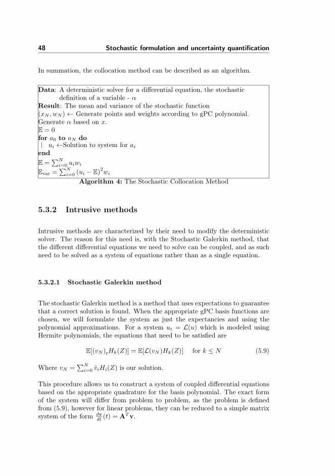
48 Stochastic formulation and uncertainty quantification
In summation, the collocation method can be described as an algorithm.
Data: A deterministic solver for a differential equation, the stochasticdefinition of a variable - α
Result: The mean and variance of the stochastic function(xN , wN )← Generate points and weights according to gPC polynomial.Generate α based on x.E = 0for a0 to aN do
ui ←Solution to system for aiendE =
∑Ni=0 uiwi
Evar =∑Ni=0 (ui − E)
2wi
Algorithm 4: The Stochastic Collocation Method
5.3.2 Intrusive methods
Intrusive methods are characterized by their need to modify the deterministicsolver. The reason for this need is, with the Stochastic Galerkin method, thatthe different differential equations we need to solve can be coupled, and as suchneed to be solved as a system of equations rather than as a single equation.
5.3.2.1 Stochastic Galerkin method
The stochastic Galerkin method is a method that uses expectations to guaranteethat a correct solution is found. When the appropriate gPC basis functions arechosen, we will formulate the system as just the expectancies and using thepolynomial approximations. For a system ut = L(u) which is modeled usingHermite polynomials, the equations that need to be satisfied are
E[(vN )tHk(Z)] = E[L(vN )Hk(Z)] for k ≤ N (5.9)
Where vN =∑Ni=0 viHi(Z) is our solution.
This procedure allows us to construct a system of coupled differential equationsbased on the appropriate quadrature for the basis polynomial. The exact formof the system will differ from problem to problem, as the problem is definedfrom (5.9), however for linear problems, they can be reduced to a simple matrixsystem of the form dv
dt (t) = ATv.
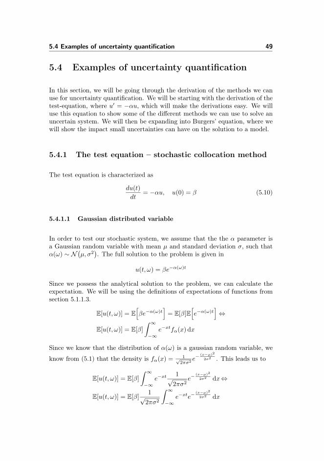
5.4 Examples of uncertainty quantification 49
5.4 Examples of uncertainty quantification
In this section, we will be going through the derivation of the methods we canuse for uncertainty quantification. We will be starting with the derivation of thetest-equation, where u′ = −αu, which will make the derivations easy. We willuse this equation to show some of the different methods we can use to solve anuncertain system. We will then be expanding into Burgers’ equation, where wewill show the impact small uncertainties can have on the solution to a model.
5.4.1 The test equation – stochastic collocation method
The test equation is characterized as
du(t)
dt= −αu, u(0) = β (5.10)
5.4.1.1 Gaussian distributed variable
In order to test our stochastic system, we assume that the the α parameter isa Gaussian random variable with mean µ and standard deviation σ, such thatα(ω) ∼ N
(µ, σ2
). The full solution to the problem is given in
u(t, ω) = βe−α(ω)t
Since we possess the analytical solution to the problem, we can calculate theexpectation. We will be using the definitions of expectations of functions fromsection 5.1.1.3.
E[u(t, ω)] = E[βe−α(ω)t
]= E[β]E
[e−α(ω)t
]⇔
E[u(t, ω)] = E[β]
∫ ∞−∞
e−xtfα(x) dx
Since we know that the distribution of α(ω) is a gaussian random variable, we
know from (5.1) that the density is fα(x) = 1√2πσ2
e−(x−µ)2
2σ2 . This leads us to
E[u(t, ω)] = E[β]
∫ ∞−∞
e−xt1√
2πσ2e−
(x−µ)2
2σ2 dx⇔
E[u(t, ω)] = E[β]1√
2πσ2
∫ ∞−∞
e−xte−(x−µ)2
2σ2 dx

50 Stochastic formulation and uncertainty quantification
Where we will solve the infinite integral using Maple
E[u(t, ω)] = E[β]1√
2πσ2e−
12 t(−tσ
2+2µ)√
2σ2π ⇔
E[u(t, ω)] = E[β]e−12 t(−tσ
2+2µ) (5.11)
We will want to calculate the variance as well, which is done by the sameprocedure as the expectation, but with the second centered moment
E[(βe−α(ω)t − E
[(βe−α(ω)t
)])2]= E
[(βe−α(ω)t − βe−
12 t(−tσ
2+2µ))2]⇔
E[(βe−α(ω)t − E
[(βe−α(ω)t
)])2]=
1√2πσ2
∫ ∞−∞
(βe−xt − βe−
12 t(−tσ
2+2µ))2e−
(x−µ)2
2σ2 dx
This is solveable in Maple, which gives us the solution
E[(βe−α(ω)t − E
[(βe−α(ω)t
)])2]= β2
(et
2σ2
− 1)e−2tµ+t
2σ2
(5.12)
(5.11) and (5.12) allows us to properly calculate the expectancy and variance,and evaluate the correctness of our solution. We will set β = 1.
As u is simply a point in time, we will not need a spectral solver for this problem.We will start by using a Monte Carlo approximation to the problem, where wewill be generating a new α(ω) for each iteration of the problem. We will becalculating the running mean for each step in the approximation, as to showconvergence. We will be generating the random parameter with the Pythonfunction numpy.random.normal
0 20000 40000 60000 80000 100000N
0.015
0.020
0.025
0.030
0.035
0.040
0.045
0.050
0.055
0.060
Running MeanExpectation
100 101 102 103 104 105
N
10-9
10-8
10-7
10-6
10-5
10-4
10-3
10-2
10-1
Error
Figure 5.2: The mean calculated by the Monte Carlo method. The runningmean is seen compared to the analytic mean in the left picture,and the running error is seen in the right picture.
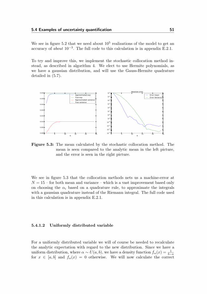
5.4 Examples of uncertainty quantification 51
We see in figure 5.2 that we need about 105 realizations of the model to get anaccuracy of about 10−3. The full code to this calculation is in appendix E.2.1.
To try and improve this, we implement the stochastic collocation method in-stead, as described in algorithm 4. We elect to use Hermite polynomials, aswe have a gaussian distribution, and will use the Gauss-Hermite quadraturedetailed in (5.7).
0 5 10 15 20 25N
0.000
0.005
0.010
0.015
0.020
0.025
0.030
0.035
Approximated expTrue expApproximated varianceTrue variance
0 5 10 15 20 25N
10-13
10-12
10-11
10-10
10-9
10-8
10-7
10-6
10-5
10-4
10-3
10-2Absolute error
Error meanError Variance
Figure 5.3: The mean calculated by the stochastic collocation method. Themean is seen compared to the analytic mean in the left picture,and the error is seen in the right picture.
We see in figure 5.3 that the collocation methods nets us a machine-error atN = 15 – for both mean and variance – which is a vast improvement based onlyon choosing the αi based on a quadrature rule, to approximate the integralswith a gaussian quadrature instead of the Riemann integral. The full code usedin this calculation is in appendix E.2.1.
5.4.1.2 Uniformly distributed variable
For a uniformly distributed variable we will of course be needed to recalculatethe analytic expectation with regard to the new distribution. Since we have auniform distribution, where α ∼ U(a, b), we have a density function fα(x) = 1
b−afor x ∈ [a, b] and fα(x) = 0 otherwise. We will now calculate the correct

52 Stochastic formulation and uncertainty quantification
expectation.
E[u(t)] = E[β]
∫ ∞−∞
e−xtfα(x) dx⇔
E[u(t)] = E[β]
∫ b
a
e−xt1
b− adx⇔
E[u(t)] = E[β]1
b− a
∫ b
a
e−xt dx⇔
E[u(t)] = E[β]1
b− ae−at − e−bt
t
Using this, we will repeat the above exercise using Monte Carlo method infigure 5.4, for α ∼ U(−7, 2)
0 20000 40000 60000 80000 100000N
1
2
3
4
5
6
7
8
9
10
Running MeanExpectation
100 101 102 103 104 105
N
10-6
10-5
10-4
10-3
10-2
10-1
100
101
Error
Figure 5.4: The mean calculated by the Monte Carlo method on a uniformdistribution. The running mean is seen compared to the analyticmean in the left picture, and the running error is seen in the rightpicture.
The full code for the calculation can be found in appendix E.2.1.
For the stochastic collocation method, we will be using Legendre polynomials,and the Legendre-Gauss quadrature detailed in (5.8).
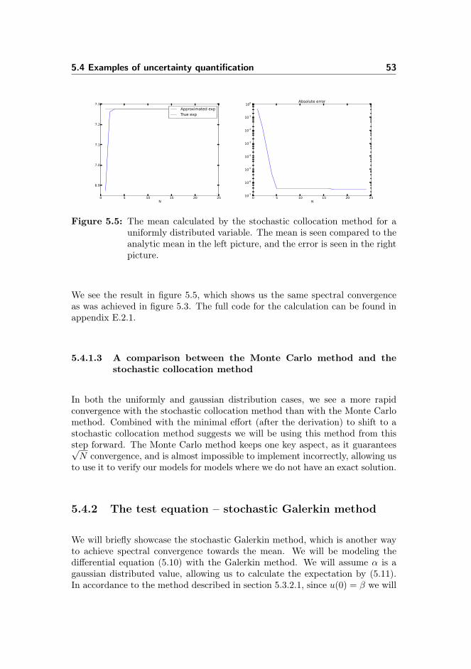
5.4 Examples of uncertainty quantification 53
0 5 10 15 20 25N
6.9
7.0
7.1
7.2
7.3
Approximated expTrue exp
0 5 10 15 20 25N
10-7
10-6
10-5
10-4
10-3
10-2
10-1
100 Absolute error
Figure 5.5: The mean calculated by the stochastic collocation method for auniformly distributed variable. The mean is seen compared to theanalytic mean in the left picture, and the error is seen in the rightpicture.
We see the result in figure 5.5, which shows us the same spectral convergenceas was achieved in figure 5.3. The full code for the calculation can be found inappendix E.2.1.
5.4.1.3 A comparison between the Monte Carlo method and thestochastic collocation method
In both the uniformly and gaussian distribution cases, we see a more rapidconvergence with the stochastic collocation method than with the Monte Carlomethod. Combined with the minimal effort (after the derivation) to shift to astochastic collocation method suggests we will be using this method from thisstep forward. The Monte Carlo method keeps one key aspect, as it guarantees√N convergence, and is almost impossible to implement incorrectly, allowing us
to use it to verify our models for models where we do not have an exact solution.
5.4.2 The test equation – stochastic Galerkin method
We will briefly showcase the stochastic Galerkin method, which is another wayto achieve spectral convergence towards the mean. We will be modeling thedifferential equation (5.10) with the Galerkin method. We will assume α is agaussian distributed value, allowing us to calculate the expectation by (5.11).In accordance to the method described in section 5.3.2.1, since u(0) = β we will

54 Stochastic formulation and uncertainty quantification
be seeking a solution
vN =
N∑i=0
viHi(Z)
where
αN =
N∑i=0
aiHi(Z) βN =
N∑i=0
biHi(Z)
We can truncate the last two sums, as only the two first ais are defined as notzero - as a0 = µ and a1 = σ - as well as the first bi - b0 = β. Using the Galerkinmethod, we acquire the formulation of the system
E[dvndt
Hk(Z)
]= E[−αNvNHk(Z)] for k = 0, . . . , N
If we substitute our gPC approximations into this system, we get
E
ddt
N∑j=0
vjHj(Z)Hk(Z)
= E
− N∑i=0
aiHi(Z)
N∑j=0
vjHj(Z)Hk(Z)
for k = 0, . . . , N
Where we can draw the coefficients out, since they are not affecting the calcu-lation of the expectancy.
d
dt
N∑j=0
vjE[Hj(Z)Hk(Z)] = −N∑i=0
N∑j=0
aivjE[Hi(Z)Hj(Z)Hk(Z)] for k = 0, . . . , N
Since we know our basis functions have the orthogonality quality described in(5.2), we can reduce the right-hand side of the equation
d
dtvkγk = −
N∑i=0
N∑j=0
aivjE[Hi(Z)Hj(Z)Hk(Z)] for k = 0, . . . , N ⇔
d
dtvk =
−1
γk
N∑i=0
N∑j=0
aivjE[Hi(Z)Hj(Z)Hk(Z)] for k = 0, . . . , N
We know that γk = E[H2k(Z)
], but we will use the analytical version shown in
[Xiu10, Eq. 6.8], as γk = k! for Hermite polynomials. We can use Gauss-Hermitequadrature to calculate the expectancy from the right-hands side, as
eijk = E[Hi(Z)Hj(Z)Hk(Z)] =
∫ ∞−∞
Hi(Z)Hj(Z)Hk(Z)dFZ(z)⇔
eijk =
M∑m=0
Hi(zm)Hj(zm)Hk(zm)wm
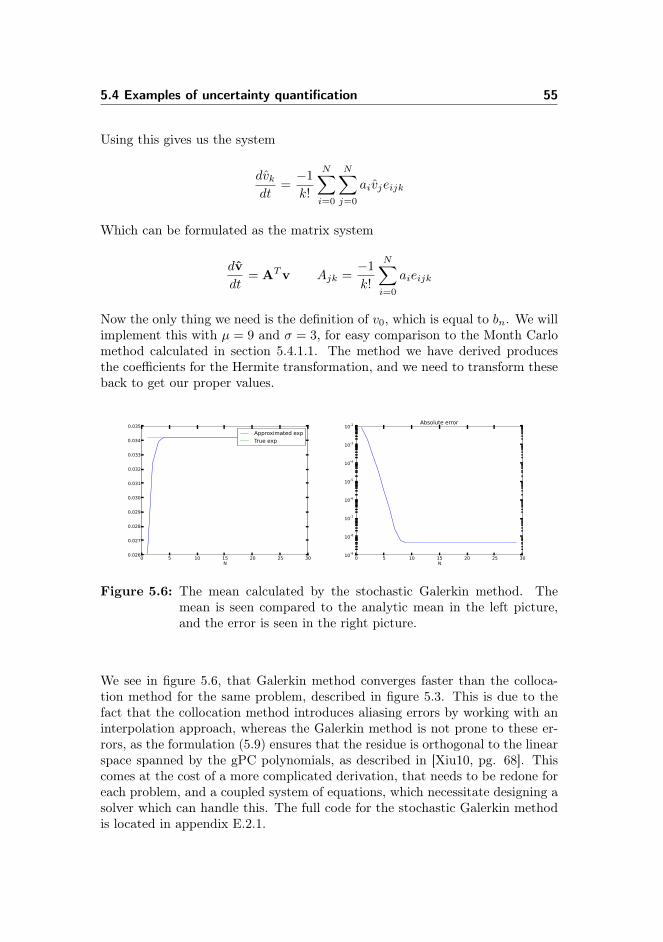
5.4 Examples of uncertainty quantification 55
Using this gives us the system
dvkdt
=−1
k!
N∑i=0
N∑j=0
aivjeijk
Which can be formulated as the matrix system
dv
dt= ATv Ajk =
−1
k!
N∑i=0
aieijk
Now the only thing we need is the definition of v0, which is equal to bn. We willimplement this with µ = 9 and σ = 3, for easy comparison to the Month Carlomethod calculated in section 5.4.1.1. The method we have derived producesthe coefficients for the Hermite transformation, and we need to transform theseback to get our proper values.
0 5 10 15 20 25 30N
0.026
0.027
0.028
0.029
0.030
0.031
0.032
0.033
0.034
0.035
Approximated expTrue exp
0 5 10 15 20 25 30N
10-9
10-8
10-7
10-6
10-5
10-4
10-3
10-2Absolute error
Figure 5.6: The mean calculated by the stochastic Galerkin method. Themean is seen compared to the analytic mean in the left picture,and the error is seen in the right picture.
We see in figure 5.6, that Galerkin method converges faster than the colloca-tion method for the same problem, described in figure 5.3. This is due to thefact that the collocation method introduces aliasing errors by working with aninterpolation approach, whereas the Galerkin method is not prone to these er-rors, as the formulation (5.9) ensures that the residue is orthogonal to the linearspace spanned by the gPC polynomials, as described in [Xiu10, pg. 68]. Thiscomes at the cost of a more complicated derivation, that needs to be redone foreach problem, and a coupled system of equations, which necessitate designing asolver which can handle this. The full code for the stochastic Galerkin methodis located in appendix E.2.1.

56 Stochastic formulation and uncertainty quantification
5.4.3 Burgers’ equation – the influence of uncertainty
We recall the viscous Burgers’ equation from section 3.3.2
ut + uux = vuxx x ∈ [−1, 1]
u(−1, t) = 1 u(1, t) = −1 ,∀t > 0
v > 0
With the initial condition u(x, 0) = −tanh(x) 1|−tanh(−1)|
We saw in figure 4.5 that the solution assumes a steady state which features asteady curve with a rapid shift in the middle of the spectrum.
5.4.3.1 Introducing uncertainty
To introduce uncertainty, we will make the value of v uncertain, as it will allowus to model the problem the same way we modeled it for the test equation,and we will use the stochastic collocation method to approximate the stochasticvariable. We will let v attain a uniform distribution, since we know that vmust always be greater than zero, disallowing us to model it with a gaussianvariable. This gives us v U(0.05, 0.2), which allows us to model the uncertaintyover v. We will implement the uncertainty dimension much as we would with a2-dimensional spectral method, using one vector to represent all the solutions,and reforming the solution afterwards. This will require some code-wise tricksdescribed in section 4.3.3.1.
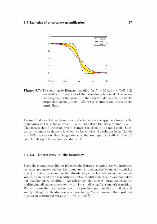
5.4 Examples of uncertainty quantification 57
−1.0 −0.5 0.0 0.5 1.0−1.5
−1.0
−0.5
0.0
0.5
1.0
1.5
UpperExpLow
Figure 5.7: The solution to Burgers’ equation for N = 60 and v U(0.05, 0.2)modeled by 10 iterations of the Legendre polynomial. The yellowband represents the mean µ ± the standard derivation σ, and thepurple lines define µ± 2σ. 95% of the solutions will be inside thepurple lines.
Figure 5.7 shows that variation over v affects neither the approach towards theboundaries or the point at which u = 0, but rather the slope around u = 0.This means that a variation over v changes the slope of the rapid shift. Sincewe can compare to figure 4.5, where we know what the solution looks like forv = 0.05, we can say that the greater v is, the less rapid the shift is. The fullcode for this problem is in appendix E.2.2
5.4.3.2 Uncertainty on the boundary
Since the v parameter did not influence the Burgers’ equation, we will introducean extra parameter on the left boundary, ε, making the boundary conditionu(−1) = 1 + ε. Since our model already keeps the boundaries as their initialvalues, all we need to to is modify the initial condition in order to accommodateour new boundary condition. We will adjust the current initial condition, bymultiplying all values above zero with (1 + ε), allowing for a smooth transition.We will reuse the construction from the previous part, setting v = 0.05, andsimply letting ε be the dimension of uncertainty. We will assume that epsilon isa gaussian distributed variable ε ∼ N
(0.1, 0.052
).
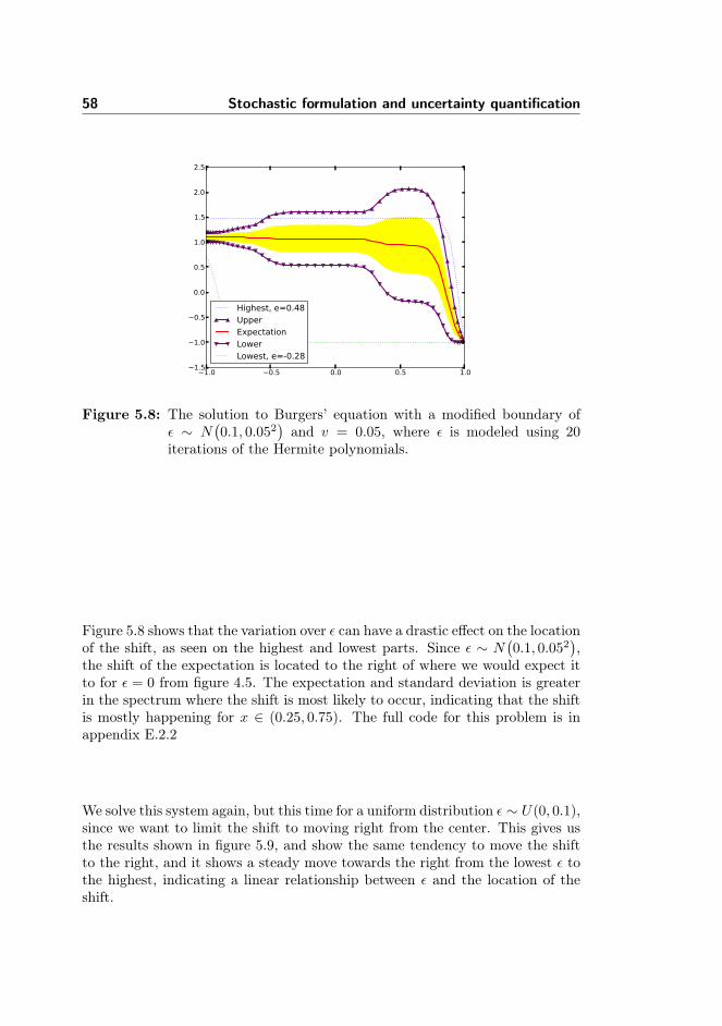
58 Stochastic formulation and uncertainty quantification
−1.0 −0.5 0.0 0.5 1.0−1.5
−1.0
−0.5
0.0
0.5
1.0
1.5
2.0
2.5
Highest, e=0.48UpperExpectationLowerLowest, e=-0.28
Figure 5.8: The solution to Burgers’ equation with a modified boundary ofε ∼ N
(0.1, 0.052
)and v = 0.05, where ε is modeled using 20
iterations of the Hermite polynomials.
Figure 5.8 shows that the variation over ε can have a drastic effect on the locationof the shift, as seen on the highest and lowest parts. Since ε ∼ N
(0.1, 0.052
),
the shift of the expectation is located to the right of where we would expect itto for ε = 0 from figure 4.5. The expectation and standard deviation is greaterin the spectrum where the shift is most likely to occur, indicating that the shiftis mostly happening for x ∈ (0.25, 0.75). The full code for this problem is inappendix E.2.2
We solve this system again, but this time for a uniform distribution ε ∼ U(0, 0.1),since we want to limit the shift to moving right from the center. This gives usthe results shown in figure 5.9, and show the same tendency to move the shiftto the right, and it shows a steady move towards the right from the lowest ε tothe highest, indicating a linear relationship between ε and the location of theshift.
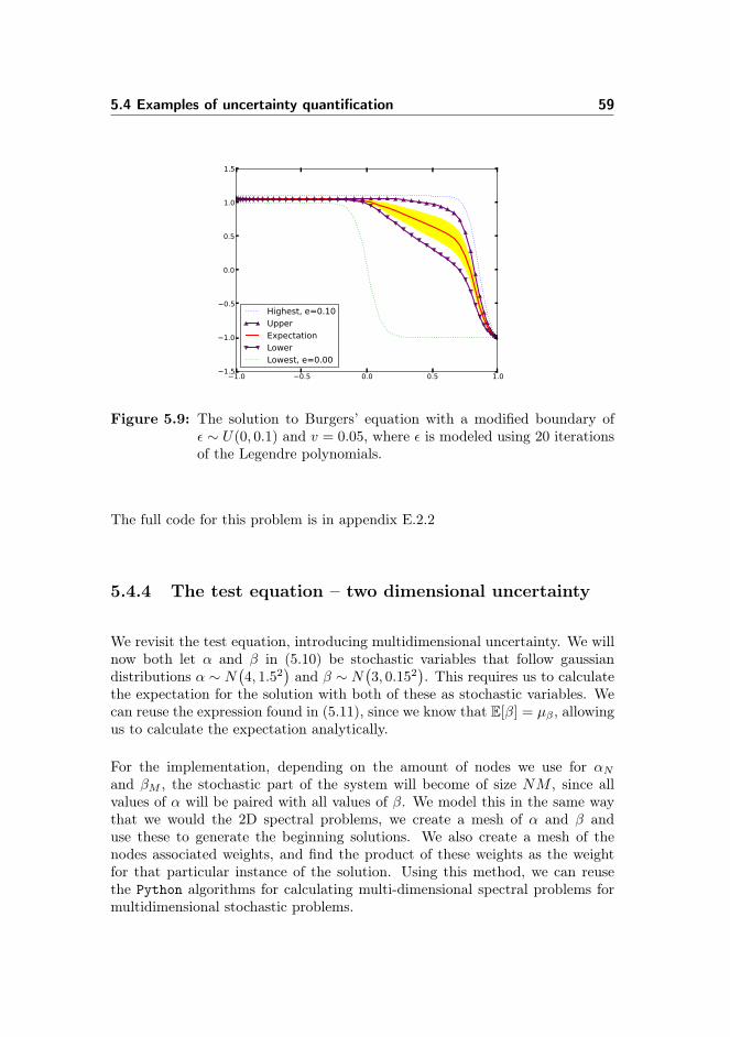
5.4 Examples of uncertainty quantification 59
−1.0 −0.5 0.0 0.5 1.0−1.5
−1.0
−0.5
0.0
0.5
1.0
1.5
Highest, e=0.10UpperExpectationLowerLowest, e=0.00
Figure 5.9: The solution to Burgers’ equation with a modified boundary ofε ∼ U(0, 0.1) and v = 0.05, where ε is modeled using 20 iterationsof the Legendre polynomials.
The full code for this problem is in appendix E.2.2
5.4.4 The test equation – two dimensional uncertainty
We revisit the test equation, introducing multidimensional uncertainty. We willnow both let α and β in (5.10) be stochastic variables that follow gaussiandistributions α ∼ N
(4, 1.52
)and β ∼ N
(3, 0.152
). This requires us to calculate
the expectation for the solution with both of these as stochastic variables. Wecan reuse the expression found in (5.11), since we know that E[β] = µβ , allowingus to calculate the expectation analytically.
For the implementation, depending on the amount of nodes we use for αNand βM , the stochastic part of the system will become of size NM , since allvalues of α will be paired with all values of β. We model this in the same waythat we would the 2D spectral problems, we create a mesh of α and β anduse these to generate the beginning solutions. We also create a mesh of thenodes associated weights, and find the product of these weights as the weightfor that particular instance of the solution. Using this method, we can reusethe Python algorithms for calculating multi-dimensional spectral problems formultidimensional stochastic problems.

60 Stochastic formulation and uncertainty quantification
0.0 0.1 0.2 0.3 0.4 0.5t
−0.5
0.0
0.5
1.0
1.5
2.0
2.5
3.0
3.5
UpperMeanLower
Figure 5.10: The solution to 2-dimensional uncertainty applied to the testequation.
0 5 10 15 20 25N
0.524
0.526
0.528
0.530
0.532
0.534
0.536
0.538
Approximated expTrue exp
0 5 10 15 20 25N
10-12
10-11
10-10
10-9
10-8
10-7
10-6
10-5
10-4
10-3
10-2
10-1Absolute error
Figure 5.11: The approximated expectation and the error of the expectationas a function of the size of our samples.
We see from figure 5.11 that we conserve the fast spectral convergence for mul-tiple dimensions of uncertainty, and we can see in figure 5.10 that in the startthe variation seems to be controlled by the β uncertainty, but as t gets bigger,the variation rises due to the great effect of negative values of α.
The entire code for this problem can be found in appendix E.2.1.
While we will not be using this method from this point on, it is worth notingthat the stochastic collocation method is easily expanded to increase the numberof random parameters.

Chapter 6
Numerical experiments
In this chapter we will focus on pseudo-practical applications of the uncertaintyquantification and spectral methods developed in this book. We will concernourselves with two problems, a lid driven cavity problem, and a wave modelsimulator.
6.1 Lid driven cavity
The lid driven cavity problem aims to describe the flow in a container, wherethe lid is driving the flow in a certain direction, as if to simulate the flowwithin a cavity where a steady stream is passing over. The lid driven cavityproblem comes from the non-dimensional steady-state Navier-Stokes equationsfor incompressible flow as described in [WZ10], which we will be employing ona physical domain Ω = [0, 1]× [0, 1]..
∇ · u = 0 (6.1)
(u · ∇)u = −∇p+Re−1∇2u (6.2)
Here each point is represented by the velocity u = (u, v), where u and v arethe velocity components in the respectively x- and y-direction. Each point also

62 Numerical experiments
has a value of the pressure p associated with it, but only on the interior nodes,in order to eliminate the need for boundary conditions and the possibility ofpollution from nonphysical modes [WZ10]. Re is the Reynolds number, whichis defined as Vchd/ν, which is found by choosing the characteristic velocity Vch– or the speed of the lid – and length d, with ν being the kinematic viscosity.
The problem will be formulated with Dirichlet boundaries, where (u, v) = (0, 0)on all boundaries for the top boundary, where u = 1.
In order to achieve the steady state, we will introduce pseudo-time variables τ ,which will detail the initial-value-problem we will ned to step through.
1
β2
∂p
∂τ+∇ · u = 0 (6.3)
∂u
∂τ+ (u · ∇)u = −∇p+Re−1∇2u (6.4)
Where β2 = 5 is chosen in [WZ10], and since this will not affect the final result,we will choose this as well.
With the model we will seek to examine the influence of uncertainty in the lid-speed, represented through the Reynolds number, and how the stream in thecavity is effected by this.
6.1.1 Derivation of the spectral model
We will be employing the Legendre spectral collocation method to solve thisinitial-value problem. Since we are employing Dirichlet boundaries, we will beusing Legendre polynomials to model both dimensions, both for the full (u, v)grid, as with the inner p grid.
6.1.1.1 Scaling the working grid
This means that with the original Legendre grid xL, yL ∈ [−1, 1] we will needto employ the transformation to xN , yN ∈ [0, 1].
xN =xL + 1
2yN =
yL + 1
2
Which gives us the scaling factors of
dxLdxN
= 2dyLdyN
= 2 (6.5)

6.1 Lid driven cavity 63
Since the pressure p is also modeled by Legendre polynomials, but is connectedto the inner grid of points xi, yi for 1 ≤ i ≤ N − 1, we will need to scale thesepoints as well to xN−2, yN−2 ∈ [−1, 1]. This is easily done with
xi =xixc
yi =yiyc
for 1 ≤ i ≤ N − 1 ∧ c = N − 1 (6.6)
Which will give us the secondary1 scaling factor ofdxidxi
= xcdyidyi
= yc for 1 ≤ i ≤ N − 1 ∧ c = N − 1 (6.7)
6.1.1.2 Using the collocation approximation
Now all we need to do is define the equations (6.3) and (6.4) in the collocationapproximation. Since u = (u, v), we can write the divergence as
∇ · u =
( ddxddy
)·
(u
v
)=du
dx+dv
dx
Which means that we can approximate this using the collocation differentiationoperator
∇ · uN = DxuN +DyvN
This will allow us to formulate the continuity equation (6.3) from the system as
1
β2
∂pN∂τ
+∇ · uN = 0⇔
∂pN∂τ
= −β2(∇ · uN )⇔
∂pN∂τ
= −β2(DxuN +DyvN ) (6.8)
In order to approximate the momentum equation (6.4), we will need to calculatethe Laplacian ∇2u and the convection (u · ∇)u. The Laplacian will be
∇2u =
((ddxddy
)·
(ddxddy
))(u
v
)⇔
∇2u =
(d2
dx2+
d2
dy2
)(u
v
)⇔
∇2u =
(d2udx2 + d2u
dv2
d2vdx2 + d2v
dv2
)(6.9)
1Since we will also need to apply the scaling factor from (6.5)

64 Numerical experiments
And the convection
(u · ∇)u =
((u
v
)·
(ddxddy
))(u
v
)⇔
(u · ∇)u =
(ud
dx+ v
d
dy
)(u
v
)⇔
(u · ∇)u =
(ududx + v dudyu dvdx + v dvdy
)(6.10)
(6.9) and (6.10) allows us to formulate the momentum equation for our model
∂u
∂τ+ (u · ∇)u = −∇p+Re−1∇2u⇔
∂u
∂τ= −(u · ∇)u−∇p+Re−1∇2u⇔
∂u
∂τ= −
(ududx + v dudyu dvdx + v dvdy
)−
(dpdxdpdy
)+
(d2udx2 + d2u
dy2
d2vdx2 + d2v
dy2
)
Which we can also approximate using the collocation approximation
du
dτ= −(uDxu+ vDyu)− dpN−2
dx+D2
xu+D2yu (6.11)
dv
dτ= −(uDxv + vDyv)− dpN−2
dy+D2
xv +D2yv (6.12)
The reason why we have not used a differential operator to approximate ∇p isthat p is only defined on the inner grid, and thus approximated by pN−2. Wewill need to differentiate this on the inner grid, and then interpolate the valuesto the full grid.
6.1.1.3 Interpolating the pressure
The pressure will be modeled by the inner grid with pN−2. Since we calculatethe τ differential in (6.8), we will simply only apply the inner-grid values ofthis differential, and disregard the outer grid completely. For the equations(6.11) and (6.12) however, we will need the space derivative of the pressure forapplication on the full grid – and we will need to interpolate the values fromthe inner grid to the outer grid for this.
We will be using the Vandermonde matrix as defined in (3.6), since it can trans-form the nodal values to the modal values. Once we have the modal values, we
6.1 Lid driven cavity 65
can interpolate these to the outer grid nodal values using another Vandermondematrix. The second Vandermonde matrix will need to be defined on the innergrid extrapolated to the outer values, which means that we will have to reversethe scaling, giving us
xN = xNxc yN = yNyc c = N − 1 (6.13)
This allows us to interpolate the pressure using the functions
pN−2 = V1pN−2 ⇔ pN−2 = V −11 pN−2
pN = V2pN−2
This requires the p values to be allocated into a vector, with the Vandermondematrix V1 being of size (N − 2)
2 × (N − 2)2, while V2 will be of size N2 ×
(N − 2)2.
In order to calculate these Vandermonde matrices, we will use the same methodas we used for the differential operators in section 4.3.3.2, and create the Van-dermonde for the x-direction and the y-direction independently using the pointsxN−2 and yN−2, then creating V1 = VxN−2
⊗ VyN−2. For the second Vander-
monde matrix, we will be creating the Vandermonde matrices using the pointsxN and yN , and then creating V2 = VxN ⊗ VyN .
This allows us to define the interpolation as
∇pN = V2V−11 ∇pN−2
Where ∇pN−2 is found with the differential operator defined on the inner grid.
6.1.1.4 Applying the boundary conditions
Since we are working with nodal points and a collocation approximation, we willsimply ensure that the points on the boundary fulfill the boundary conditions,this being that (u, v) = (0, 0) on all boundaries, except where y = 1, where theboundary is (u, v) = (1, 0). The pressure has no boundary conditions as it isonly defined on the inner grid.
6.1.1.5 The τ-steps
For the time stepping procedure we will be using the explicit four-stage Runge-Kutta method, as it is used in [WZ10], where the time step to guarantee con-vergence is supplied. This means that we will be using the following method

66 Numerical experiments
φ(1) = φn +1
4∆τR(φn)
φ(2) = φn +1
3∆τR
(φ(1)
)φ(3) = φn +
1
2∆τR
(φ(2)
)φ(n+1) = φn + ∆τR
(φ(3)
)(6.14)
Where the R(•) is the right-hand-side function, which is defined independentlyfor u, v and p from (6.11), (6.11) and (6.8).
The pseudo-time steps are defined by
∆τ =CFL
λx + λy(6.15)
Where CFL is the Courant-Friedrichs-Lewy’s number, which we will set to 0.5,and the λs are the limits contributed by the Navier-Stokes equations, which arecalculated as
λx =|umax|+
√u2max + β2
∆x+
1
Re ·∆x2
λy =|vmax|+
√v2max + β2
∆y+
1
Re ·∆y2
Where ∆x and ∆y are the minimum collocation spacing on their respectivegrids.
6.1.2 Implementation of the spectral model
The implementation of the spectral model is necessary to examine the influenceof the Reynolds-number, and we will develop a model for Re = 100, where wehave results to compare against from [WZ10].
6.1.2.1 Generation of points and differential matrices
Since we will be using Legendre polynomials to model the data, we will be gener-ating the points for the outer grid with the function GaussLobattoQuadraturefrom DABISpectral1D. One these points are generated, we will calculate the
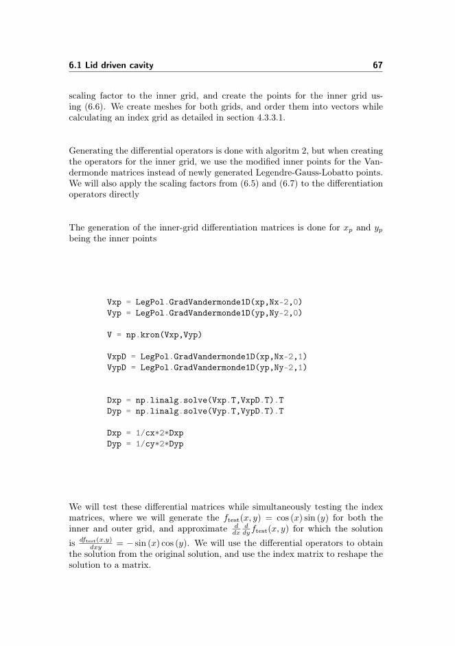
6.1 Lid driven cavity 67
scaling factor to the inner grid, and create the points for the inner grid us-ing (6.6). We create meshes for both grids, and order them into vectors whilecalculating an index grid as detailed in section 4.3.3.1.
Generating the differential operators is done with algoritm 2, but when creatingthe operators for the inner grid, we use the modified inner points for the Van-dermonde matrices instead of newly generated Legendre-Gauss-Lobatto points.We will also apply the scaling factors from (6.5) and (6.7) to the differentiationoperators directly
The generation of the inner-grid differentiation matrices is done for xp and ypbeing the inner points
Vxp = LegPol.GradVandermonde1D(xp,Nx-2,0)Vyp = LegPol.GradVandermonde1D(yp,Ny-2,0)
V = np.kron(Vxp,Vyp)
VxpD = LegPol.GradVandermonde1D(xp,Nx-2,1)VypD = LegPol.GradVandermonde1D(yp,Ny-2,1)
Dxp = np.linalg.solve(Vxp.T,VxpD.T).TDyp = np.linalg.solve(Vyp.T,VypD.T).T
Dxp = 1/cx*2*DxpDyp = 1/cy*2*Dyp
We will test these differential matrices while simultaneously testing the indexmatrices, where we will generate the ftest(x, y) = cos (x) sin (y) for both theinner and outer grid, and approximate d
dxddyftest(x, y) for which the solution
is dftest(x,y)dxy = − sin (x) cos (y). We will use the differential operators to obtain
the solution from the original solution, and use the index matrix to reshape thesolution to a matrix.

68 Numerical experiments
0.0 0.2 0.4 0.6 0.8 1.0x
0.0
0.2
0.4
0.6
0.8
1.0
y
Differentiation test, error for full grid
0.0
0.8
1.6
2.4
3.2
4.0
4.8
5.6
6.4
7.2
1e−11
0.0 0.2 0.4 0.6 0.8 1.0x
0.0
0.2
0.4
0.6
0.8
1.0
y
Differentiation test, error for inner grid
0.0
0.5
1.0
1.5
2.0
2.5
3.0
3.5
4.0
4.5
1e−10
Figure 6.1: The errors of our differential approximation test, the full grid tothe left, and the inner grid to the right
As we can see from figure 6.1, the errors for both test cases are acceptable, andwe can consider these methods implemented correctly. The full script for testingthe errors is featured in the approximation script in appendix F.1.
6.1.2.2 Interpolation of points from the inner grid
The generation of the matrices to interpolate from the inner grid to the outer gridwill rely on Vandermonde matrices generated by the function GradVandermondefrom DABISpectral1D. The matrix V1 is calculated as a standard Vandermondematrix for the points on the inner grid, while the matrix V2 is generated as astandard Vandermonde matrix for the inner grid, but with the scaled pointsfrom (6.13).
In order to test the interpolation, we create the grid of a function exy, whichwe interpolate from the inner grid to the outer grid, and compare to the correctvalues on the outer grid.
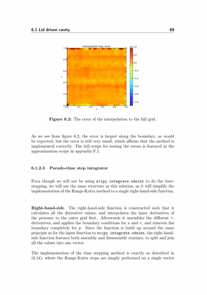
6.1 Lid driven cavity 69
0.0 0.2 0.4 0.6 0.8 1.0x
0.0
0.2
0.4
0.6
0.8
1.0
y
Interpolation test, error
−1.0
−0.8
−0.6
−0.4
−0.2
0.0
0.2
1e−12
Figure 6.2: The error of the interpolation to the full grid.
As we see from figure 6.2, the error is largest along the boundary, as wouldbe expected, but the error is still very small, which affirms that the method isimplemented correctly. The full script for testing the errors is featured in theapproximation script in appendix F.1.
6.1.2.3 Pseudo-time step integrator
Even though we will not be using scipy.integrate.odeint to do the time-stepping, we will use the same structure as this solution, as it will simplify theimplementation of the Runge-Kutta method to a single right-hand-side function.
Right-hand-side The right-hand-side function is constructed such that itcalculates all the derivative values, and interpolates the inner derivatives ofthe pressure to the outer grid first. Afterwards it assembles the different τ -derivatives, and applies the boundary conditions for u and v, and removes theboundary completely for p. Since the function is build up around the sameprinciple as for the input function to scipy.integrate.odeint, the right-hand-side function features both assembly and disassembly routines, to split and joinall the values into one vector.
The implementation of the time stepping method is exactly as described in(6.14), where the Runge-Kutta steps are simply performed on a single vector
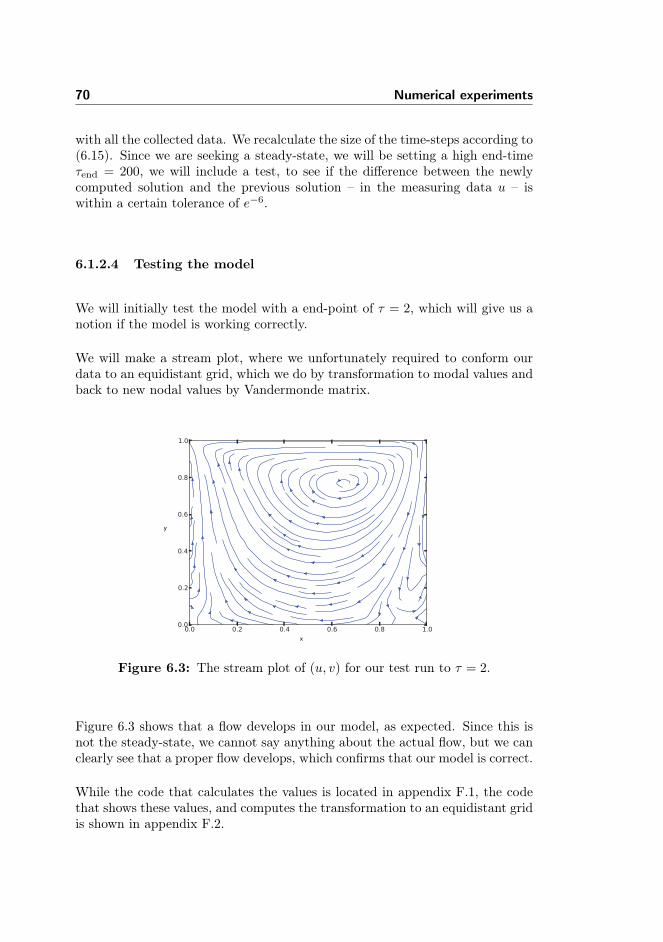
70 Numerical experiments
with all the collected data. We recalculate the size of the time-steps according to(6.15). Since we are seeking a steady-state, we will be setting a high end-timeτend = 200, we will include a test, to see if the difference between the newlycomputed solution and the previous solution – in the measuring data u – iswithin a certain tolerance of e−6.
6.1.2.4 Testing the model
We will initially test the model with a end-point of τ = 2, which will give us anotion if the model is working correctly.
We will make a stream plot, where we unfortunately required to conform ourdata to an equidistant grid, which we do by transformation to modal values andback to new nodal values by Vandermonde matrix.
y
x
Figure 6.3: The stream plot of (u, v) for our test run to τ = 2.
Figure 6.3 shows that a flow develops in our model, as expected. Since this isnot the steady-state, we cannot say anything about the actual flow, but we canclearly see that a proper flow develops, which confirms that our model is correct.
While the code that calculates the values is located in appendix F.1, the codethat shows these values, and computes the transformation to an equidistant gridis shown in appendix F.2.

6.1 Lid driven cavity 71
6.1.3 Introducing uncertainty on the Reynolds number
We wish to introduce uncertainty in the surface speed, which will effectivelychange the Reynolds number, and investigate how the values affects our compu-tations. This is done by the stochastic collocation method, where we can simplyrun the model several times, for the calculated values of our new Reynolds num-bers, where we will compare the results to the velocity profile of u along themiddle of the cavity in the y-axis direction. Since the problem is normalized toa speed of u = 1 along the upper boundary, this will not change.
We will use a modified solver, which simply runs the problem several timeswith different Reynolds numbers, and saves each output. Each run is assigneda weight according to the GPC polynomial, and mean and variance are foundusing the different weighted values.
We do a test run for Re ∼ N(100, 102
), and let it run to τ = 1, just to see if we
are able to quantify the change in the values.
u
y
Figure 6.4: The test for our uncertainty quantification run of the lid drivencavity problem
Figure 6.4 shows us that while the uncertainty in not very pronounced, thatthere is a difference between the highest and lowest values of Re, but that ingeneral the solution will not change much for Re ∼ N
(100, 102
). The code for
this run can be found in appendix F.1.

72 Numerical experiments
6.1.4 Numerical experiments with UQ on the Reynoldsnumber
We have results from [UG82], for the velocity profile of u down the middle ofthe cavity at certain points for Re = [100, 400, 1000], which we will take as ameasure for the correctness of our model.
We will start by running from the initial condition (u, v, p) = (0, 0, 1) on theinner grid, and approximating the results from [UG82] with the same Reynoldsnumbers. This will serve as an initial condition for our uncertainty calculations,since it will likely be closer to the solution, saving computational time.
For our tests, since we are measuring against the velocity u, we will stop atiteration j, once our metric Mj =
‖uj−uj−1‖2‖uj−1‖2 becomes less than 10−6, which we
deem as a steady-state.
The uncertainty we will introduce will be that we have up to 5% uncertaintyin the speed of the lid for our problems – and thus a 5% uncertainty in ourReynolds number – allowing our model to quantify this uncertainty. Since wewill not be allowing more or less uncertainty, we will assume that Re is uniformlydistributed, and modeled using Legendre polynomials.
We will repeat the tests for uncertainty up to 10%, allowing us to study in whichdegree the increase in uncertainty has an impact on the propagating uncertainty.
All the scripts used in these simulations are either in appendix F.1 or ap-pendix F.2.
6.1.4.1 Uncertainty at Re = 100
The initial results for the approximation of the results from [UG82], we get thesolution shown in figure 6.5.
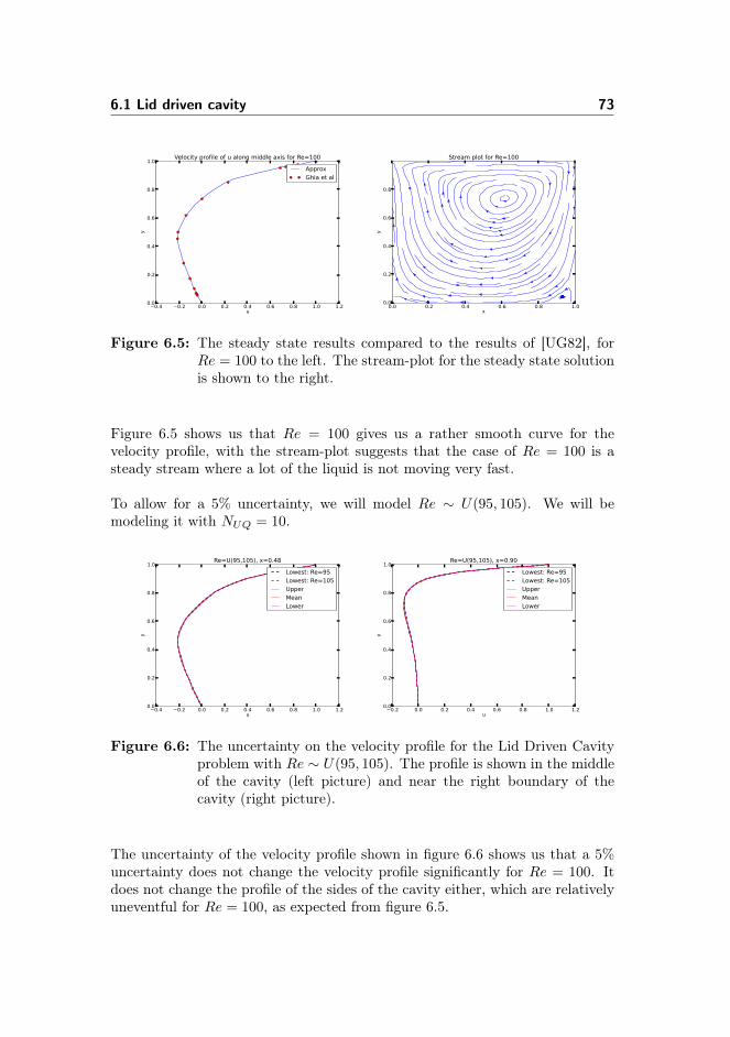
6.1 Lid driven cavity 73
−0.4 −0.2 0.0 0.2 0.4 0.6 0.8 1.0 1.2u
0.0
0.2
0.4
0.6
0.8
1.0
y
Velocity profile of u along middle axis for Re=100
ApproxGhia et al
0.0 0.2 0.4 0.6 0.8 1.0x
0.0
0.2
0.4
0.6
0.8
y
Stream plot for Re=100
Figure 6.5: The steady state results compared to the results of [UG82], forRe = 100 to the left. The stream-plot for the steady state solutionis shown to the right.
Figure 6.5 shows us that Re = 100 gives us a rather smooth curve for thevelocity profile, with the stream-plot suggests that the case of Re = 100 is asteady stream where a lot of the liquid is not moving very fast.
To allow for a 5% uncertainty, we will model Re ∼ U(95, 105). We will bemodeling it with NUQ = 10.
−0.4 −0.2 0.0 0.2 0.4 0.6 0.8 1.0 1.2u
0.0
0.2
0.4
0.6
0.8
1.0
y
Re=U(95,105), x=0.48
Lowest: Re=95Lowest: Re=105UpperMeanLower
−0.2 0.0 0.2 0.4 0.6 0.8 1.0 1.2u
0.0
0.2
0.4
0.6
0.8
1.0
y
Re=U(95,105), x=0.90
Lowest: Re=95Lowest: Re=105UpperMeanLower
Figure 6.6: The uncertainty on the velocity profile for the Lid Driven Cavityproblem with Re ∼ U(95, 105). The profile is shown in the middleof the cavity (left picture) and near the right boundary of thecavity (right picture).
The uncertainty of the velocity profile shown in figure 6.6 shows us that a 5%uncertainty does not change the velocity profile significantly for Re = 100. Itdoes not change the profile of the sides of the cavity either, which are relativelyuneventful for Re = 100, as expected from figure 6.5.
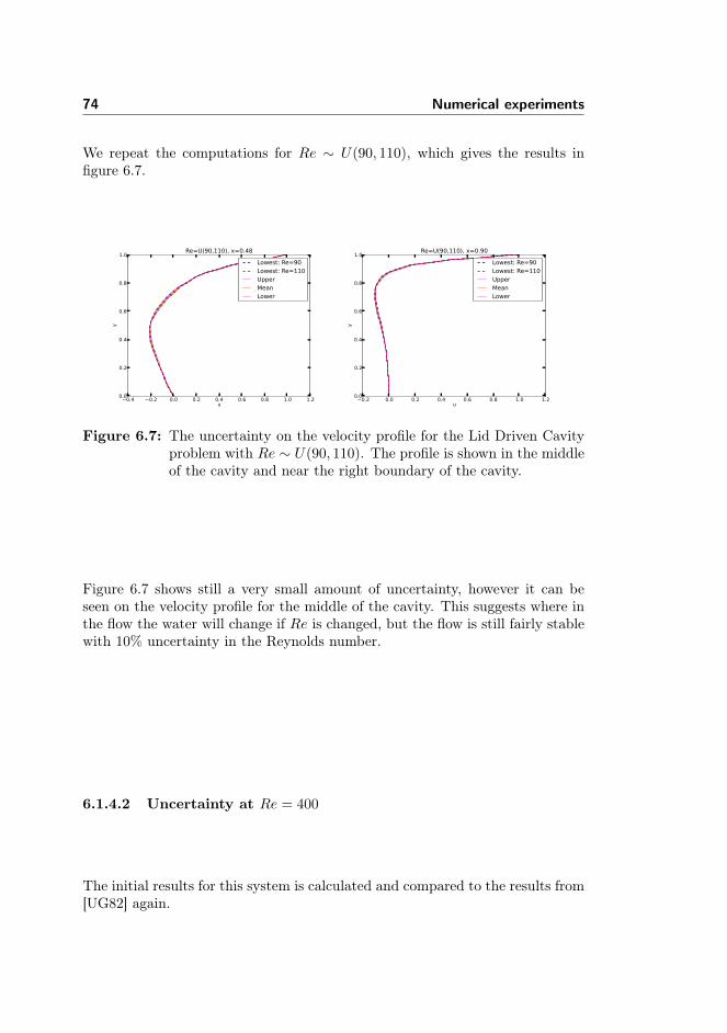
74 Numerical experiments
We repeat the computations for Re ∼ U(90, 110), which gives the results infigure 6.7.
−0.4 −0.2 0.0 0.2 0.4 0.6 0.8 1.0 1.2u
0.0
0.2
0.4
0.6
0.8
1.0
y
Re=U(90,110), x=0.48
Lowest: Re=90Lowest: Re=110UpperMeanLower
−0.2 0.0 0.2 0.4 0.6 0.8 1.0 1.2u
0.0
0.2
0.4
0.6
0.8
1.0
y
Re=U(90,110), x=0.90
Lowest: Re=90Lowest: Re=110UpperMeanLower
Figure 6.7: The uncertainty on the velocity profile for the Lid Driven Cavityproblem with Re ∼ U(90, 110). The profile is shown in the middleof the cavity and near the right boundary of the cavity.
Figure 6.7 shows still a very small amount of uncertainty, however it can beseen on the velocity profile for the middle of the cavity. This suggests where inthe flow the water will change if Re is changed, but the flow is still fairly stablewith 10% uncertainty in the Reynolds number.
6.1.4.2 Uncertainty at Re = 400
The initial results for this system is calculated and compared to the results from[UG82] again.
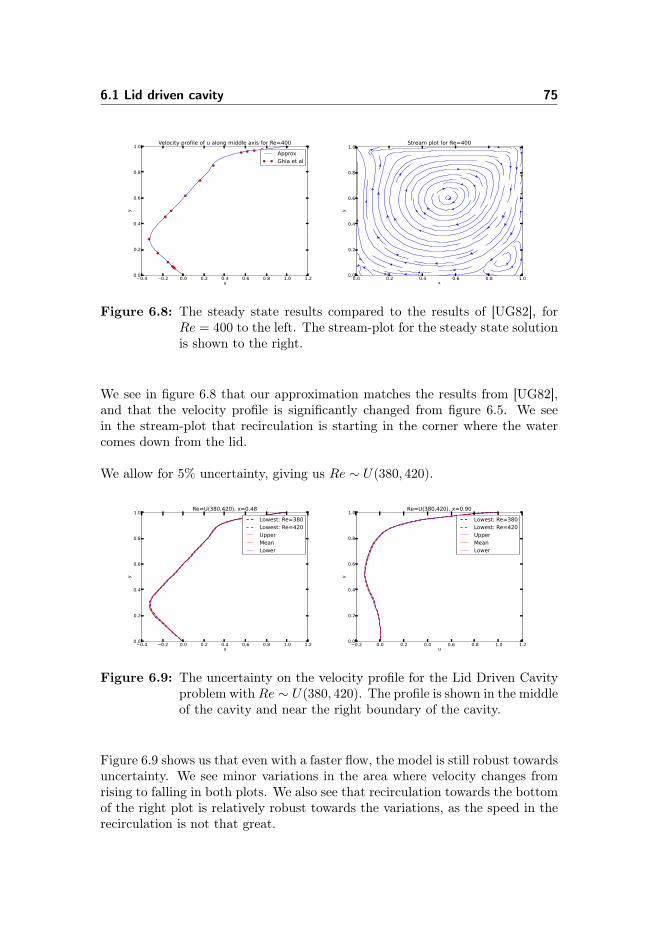
6.1 Lid driven cavity 75
−0.4 −0.2 0.0 0.2 0.4 0.6 0.8 1.0 1.2u
0.0
0.2
0.4
0.6
0.8
1.0
y
Velocity profile of u along middle axis for Re=400
ApproxGhia et al
0.0 0.2 0.4 0.6 0.8 1.0x
0.0
0.2
0.4
0.6
0.8
1.0
y
Stream plot for Re=400
Figure 6.8: The steady state results compared to the results of [UG82], forRe = 400 to the left. The stream-plot for the steady state solutionis shown to the right.
We see in figure 6.8 that our approximation matches the results from [UG82],and that the velocity profile is significantly changed from figure 6.5. We seein the stream-plot that recirculation is starting in the corner where the watercomes down from the lid.
We allow for 5% uncertainty, giving us Re ∼ U(380, 420).
−0.4 −0.2 0.0 0.2 0.4 0.6 0.8 1.0 1.2u
0.0
0.2
0.4
0.6
0.8
1.0
y
Re=U(380,420), x=0.48
Lowest: Re=380Lowest: Re=420UpperMeanLower
−0.2 0.0 0.2 0.4 0.6 0.8 1.0 1.2u
0.0
0.2
0.4
0.6
0.8
1.0
y
Re=U(380,420), x=0.90
Lowest: Re=380Lowest: Re=420UpperMeanLower
Figure 6.9: The uncertainty on the velocity profile for the Lid Driven Cavityproblem with Re ∼ U(380, 420). The profile is shown in the middleof the cavity and near the right boundary of the cavity.
Figure 6.9 shows us that even with a faster flow, the model is still robust towardsuncertainty. We see minor variations in the area where velocity changes fromrising to falling in both plots. We also see that recirculation towards the bottomof the right plot is relatively robust towards the variations, as the speed in therecirculation is not that great.
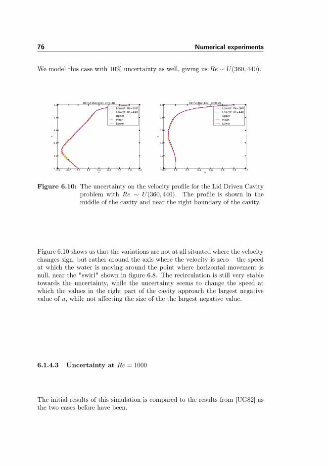
76 Numerical experiments
We model this case with 10% uncertainty as well, giving us Re ∼ U(360, 440).
−0.4 −0.2 0.0 0.2 0.4 0.6 0.8 1.0 1.2u
0.0
0.2
0.4
0.6
0.8
1.0
y
Re=U(360,440), x=0.48
Lowest: Re=360Lowest: Re=440UpperMeanLower
−0.2 0.0 0.2 0.4 0.6 0.8 1.0 1.2u
0.0
0.2
0.4
0.6
0.8
1.0
y
Re=U(360,440), x=0.90
Lowest: Re=360Lowest: Re=440UpperMeanLower
Figure 6.10: The uncertainty on the velocity profile for the Lid Driven Cavityproblem with Re ∼ U(360, 440). The profile is shown in themiddle of the cavity and near the right boundary of the cavity.
Figure 6.10 shows us that the variations are not at all situated where the velocitychanges sign, but rather around the axis where the velocity is zero – the speedat which the water is moving around the point where horizontal movement isnull, near the "swirl" shown in figure 6.8. The recirculation is still very stabletowards the uncertainty, while the uncertainty seems to change the speed atwhich the values in the right part of the cavity approach the largest negativevalue of u, while not affecting the size of the the largest negative value.
6.1.4.3 Uncertainty at Re = 1000
The initial results of this simulation is compared to the results from [UG82] asthe two cases before have been.

6.1 Lid driven cavity 77
−0.4 −0.2 0.0 0.2 0.4 0.6 0.8 1.0 1.2u
0.0
0.2
0.4
0.6
0.8
1.0
y
Velocity profile of u along middle axis for Re=1000
ApproxGhia et al
0.0 0.2 0.4 0.6 0.8 1.0x
0.0
0.2
0.4
0.6
0.8
1.0
y
Stream plot for Re=1000
Figure 6.11: The steady state results compared to the results of [UG82], forRe = 1000 to the left. The stream-plot for the steady statesolution is shown to the right.
We see in figure 6.11 that the system is now having a very well established flow.We also notice that recirculation has developed in both lower corners of thecavity. We can also verify that we have achieved the same results as [UG82]
We introduce 5% uncertainty, giving us Re ∼ U(950, 1050).
−0.4 −0.2 0.0 0.2 0.4 0.6 0.8 1.0 1.2u
0.0
0.2
0.4
0.6
0.8
1.0
y
Re=U(950,1050), x=0.48
Lowest: Re=950Lowest: Re=1050UpperMeanLower
−0.2 0.0 0.2 0.4 0.6 0.8 1.0 1.2u
0.0
0.2
0.4
0.6
0.8
1.0
y
Re=U(950,1050), x=0.90
Lowest: Re=950Lowest: Re=1050UpperMeanLower
Figure 6.12: The uncertainty on the velocity profile for the Lid Driven Cavityproblem with Re ∼ U(950, 1050). The profile is shown in themiddle of the cavity and near the right boundary of the cavity.
Figure 6.12 shows us that with this well established flow, the model is veryrobust towards uncertainty, both along the center of the cavity, and along theedges and in the recirculation zone.
We increase the uncertainty to 10%, giving us Re ∼ U(900, 1100).

78 Numerical experiments
−0.4 −0.2 0.0 0.2 0.4 0.6 0.8 1.0 1.2u
0.0
0.2
0.4
0.6
0.8
1.0
y
Re=U(900,1100), x=0.48
Lowest: Re=900Lowest: Re=1100UpperMeanLower
−0.2 0.0 0.2 0.4 0.6 0.8 1.0 1.2u
0.0
0.2
0.4
0.6
0.8
1.0
y
Re=U(900,1100), x=0.90
Lowest: Re=900Lowest: Re=1100UpperMeanLower
Figure 6.13: The uncertainty on the velocity profile for the Lid Driven Cavityproblem with Re ∼ U(900, 1100). The profile is shown in themiddle of the cavity and near the right boundary of the cavity.
Figure 6.13 shows that the uncertainty mainly focuses around the areas withthe greatest flow towards the left of the cavity, particularly the parts lower thanthese points. This indicates that the uncertainty at Re = 1000 will affect howdeep the flow manages to manifest, towards the unmoving bottom of the cavity.We again notice that even though the recirculation zone is more pronouncedthat for Re = 400, it is still very stable towards uncertainty, indicating that thiszone is not affected by the uncertainty, but driven by the overall unchangingflow.
6.1.4.4 Uncertainty at Re = 1
For Re = 1 we have no results to compare with, but run the test-case under thesame conditions that applied for the other test-cases.
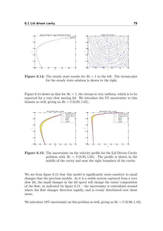
6.1 Lid driven cavity 79
−0.2 0.0 0.2 0.4 0.6 0.8 1.0u
0.0
0.2
0.4
0.6
0.8
1.0
y
Velocity profile of u along middle axis for Re=1
Approx
0.0 0.2 0.4 0.6 0.8 1.0x
0.0
0.2
0.4
0.6
0.8
1.0
y
Stream plot for Re=1
Figure 6.14: The steady state results for Re = 1 to the left. The stream-plotfor the steady state solution is shown to the right.
Figure 6.14 shows us that for Re = 1, the stream is very uniform, which is to beexpected for a very slow moving lid. We introduce the 5% uncertainty to thisdomain as well, giving us Re ∼ U(0.95, 1.05).
−0.4 −0.2 0.0 0.2 0.4 0.6 0.8 1.0 1.2u
0.0
0.2
0.4
0.6
0.8
1.0
y
Re=U(0.95,1.05), x=0.48
Lowest: Re=0Lowest: Re=1UpperMeanLower
−0.2 0.0 0.2 0.4 0.6 0.8 1.0 1.2u
0.0
0.2
0.4
0.6
0.8
1.0
y
Re=U(0.95,1.05), x=0.90
Lowest: Re=0Lowest: Re=1UpperMeanLower
Figure 6.15: The uncertainty on the velocity profile for the Lid Driven Cavityproblem with Re ∼ U(0.95, 1.05). The profile is shown in themiddle of the cavity and near the right boundary of the cavity.
We see from figure 6.15 that this model is significantly more sensitive to smallchanges that the previous models. As it is a stable system captured from a veryslow lid, the small changes in the lid speed will change the entire compositionof the flow, as indicated by figure 6.15 – the uncertainty is centralized aroundwhere the flow changes direction rapidly, and is evenly distributed over theseareas.
We introduce 10% uncertainty on this problem as well, giving usRe ∼ U(0.90, 1.10).

80 Numerical experiments
−0.4 −0.2 0.0 0.2 0.4 0.6 0.8 1.0 1.2u
0.0
0.2
0.4
0.6
0.8
1.0
y
Re=U(0.90,1.10), x=0.48
Lowest: Re=0Lowest: Re=1UpperMeanLower
−0.2 0.0 0.2 0.4 0.6 0.8 1.0 1.2u
0.0
0.2
0.4
0.6
0.8
1.0
y
Re=U(0.90,1.10), x=0.90
Lowest: Re=0Lowest: Re=1UpperMeanLower
Figure 6.16: The uncertainty on the velocity profile for the Lid Driven Cavityproblem with Re ∼ U(0.90, 1.10). The profile is shown in themiddle of the cavity and near the right boundary of the cavity.
Figure 6.16 confirms what we saw in figure 6.15, but simply expanding the areaswhere we have uncertainty. There are no significant changes otherwise.
6.1.5 Conclusions for the lid driven cavity flow model
The numerical experiments from the lid driven cavity problem shows us thatuncertainty in the input parameter can have drastically different manifestationsdependent on which state the problem is in. This means that in order to effec-tively quantify the uncertainty of a system, we will have to do active uncertaintyquantification on that system, and not simply relate to another similar prob-lem. This enhances the strength of the generalized polynomial chaos approach,as this enables us to effectively calculate the mean and standard deviation. Witha Monte-Carlo approach to this problem would we not only be unable to utilizethe last computed solution as a start in order to save computational time – theamount of times we would need to run the model would likely be unfeasiblyhigh. This would discourage the need to recompute the mean and variance fora new state of the system, and might lead to inconclusive results drawn from asimilar problem instead of computed correctly.
6.2 A nonlinear 2D wave tank model
This problem is inspired by [EK11b], and we wish to model the movement ofthe free surface, as defined by the free surface elevation η, and the surface

6.2 A nonlinear 2D wave tank model 81
scalar velocity potential φ. The model we use is a two-dimensional wave tank,illustrated in figure 6.17, and
z
(0, 0)
(−h, L) x
h
η
x1
d(x1)
x2
d(x2)
Figure 6.17: The 2D wave tank
[EK11b] describes the free surface to be governed by kinematic boundary (6.16)and dynamic boundary (6.17)
∂tη = −∂xη∂xφ+ w(
1 + (∂xη)2)
(6.16)
∂tφ = −gη − 1
2
((∂xφ
)2− w2
(1 + (∂xη)
2))
(6.17)
Where g is the gravitational acceleration, and w is the vertical velocity at thesurface.
Potential flow theory represents the velocity field as
(u
w
)=
(∂x
∂w
)φ, which we
can find by solving the two-dimensional Laplace problem
∂xxφ+ ∂zzφ = 0 − h ≤ z < η (6.18)
φ = φ z = η (6.19)(nx
nz
)·
(∂x
∂z
)φ = 0 (x, z) ∈ δΩ (6.20)
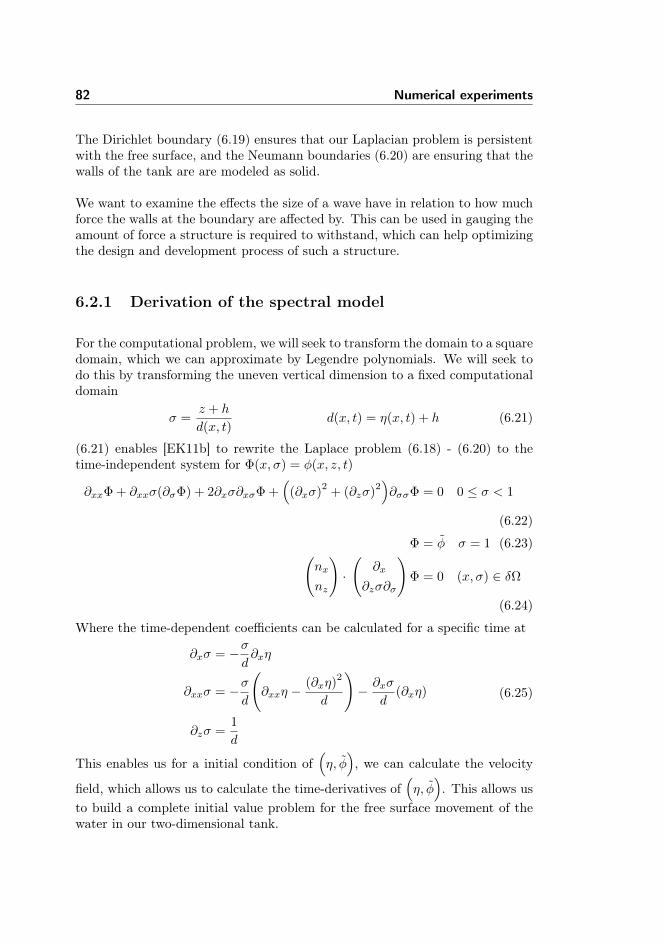
82 Numerical experiments
The Dirichlet boundary (6.19) ensures that our Laplacian problem is persistentwith the free surface, and the Neumann boundaries (6.20) are ensuring that thewalls of the tank are are modeled as solid.
We want to examine the effects the size of a wave have in relation to how muchforce the walls at the boundary are affected by. This can be used in gauging theamount of force a structure is required to withstand, which can help optimizingthe design and development process of such a structure.
6.2.1 Derivation of the spectral model
For the computational problem, we will seek to transform the domain to a squaredomain, which we can approximate by Legendre polynomials. We will seek todo this by transforming the uneven vertical dimension to a fixed computationaldomain
σ =z + h
d(x, t)d(x, t) = η(x, t) + h (6.21)
(6.21) enables [EK11b] to rewrite the Laplace problem (6.18) - (6.20) to thetime-independent system for Φ(x, σ) = φ(x, z, t)
∂xxΦ + ∂xxσ(∂σΦ) + 2∂xσ∂xσΦ +(
(∂xσ)2
+ (∂zσ)2)∂σσΦ = 0 0 ≤ σ < 1
(6.22)
Φ = φ σ = 1 (6.23)(nx
nz
)·
(∂x
∂zσ∂σ
)Φ = 0 (x, σ) ∈ δΩ
(6.24)
Where the time-dependent coefficients can be calculated for a specific time at
∂xσ = −σd∂xη
∂xxσ = −σd
(∂xxη −
(∂xη)2
d
)− ∂xσ
d(∂xη)
∂zσ =1
d
(6.25)
This enables us for a initial condition of(η, φ), we can calculate the velocity
field, which allows us to calculate the time-derivatives of(η, φ). This allows us
to build a complete initial value problem for the free surface movement of thewater in our two-dimensional tank.

6.2 A nonlinear 2D wave tank model 83
6.2.1.1 Deriving the collocation approximation
We will be using the collocation approximation with the Legendre polynomialsin both directions, allowing us to utilize the differential operators calculatedin section 3.1.2. We will be using these as single-dimensional operators in thecalculation of the time-dependent coefficients (6.25), which are calculated indi-vidually for each point in our domain.
∂xσ(x, σ) = − σ
d(x)Dxη(x)
∂xxσ(x, σ) = − σ
d(x)
(D2xη(x)− (Dxη(x))
2
2
)− Dxσ
d(x)(Dxη(x))
∂zσ(x, σ) =1
d(x)
(6.26)
Using the differential operators, we can calculate differential operators for useon the whole domain as explained in section 4.3.3.2 – where we will refer tothe differential operator in the horizontal direction as DX and in the verticaldirection as Dσ – which leads us to formulate a linear operator for solving (6.22)
L = D2X + ∂xxσDσ + 2∂xσDXDσ +
((∂xσ)
2+ (∂zσ)
2)D2σ (6.27)
LΦ = 0 (x, σ) 6∈ ∂Ω (6.28)
In order to enforce the Dirichlet boundary condition, we change the rows of Lcorresponding to the top of the grid, such that the points on the upper boundaryare exactly equal to the right-side, for which we introduce a right-hand-sidefunction
fx,σ =
φx , for σ = 1
0 , otherwise
For the Neumann boundary conditions, we modify linear operator, such thatdifferential at the outer points in the respective direction is always zero, whichis done by assigning
L = −DX for the horizontal boundariesL = −∂zσDσ for the bottom boundary
(6.29)
This allows us to calculate the velocity potential for the domain, which we canuse to calculate the time-derivatives for the free surface described in (6.16) and

84 Numerical experiments
(6.17).
∂tη = −DxηDxΦ + w(
1 + (Dxη)2)
∂tΦ = −gη − 1
2
((DxΦ
)2− w2
(1 + (Dxη)
2))
Where ∼ denotes the values at the top of the grid, and w = DσΦ.
6.2.1.2 Calculating the force on the wall
The force on the side of the domain can be calculated by an integral along thevertical axis of the pressure, according to [EK06, Eq. 2.84].
F =
∫ η
−dp(z) dz
In order to compute this, we will need to calculate the pressure on the rightboundary. This is defined in [EK06, Eq. 2.83] as
p(z)
ρ= g(η − z) +
∫ η
z
∂tw dz+1
2+(u2 − u(z)
2+ w2 − w(z)
2)
Where ρ is the density of the water, which is ρ = 0.998 and u = DXΦ. Theintegral
∫ ηz∂tw dz requires us to transform w to z points where we can utilize
the Legendre-Gauss-Lobatto quadrature, which we do by the method describedin section 6.1.1.3, by converting to modal values first, and then transforming tothe new nodal values. Since we are modelling the vertical axis by a Legendrepolynomial, we can use the Legendre-Gauss-Lobatto quadrature to calculatethe force integral, allowing us to compute F . These calculations will require atransformation of the Legendre polynomials from zL ∈ (−1, 1) to z ∈ [−h, η],which is
z =zL + 1
2(h+ η)− h
For the time-derivative of w, we will be using a simple first order approximationfor the time-derivative.
6.2.2 Implementation of the spectral model
The implementation of the spectral model will consist of three parts, a solverfor our Laplace problem, the integrator for the time-dependent problem, and acalculation of the pressure.
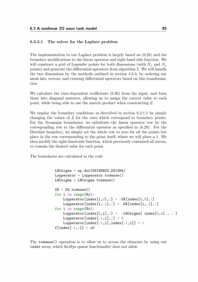
6.2 A nonlinear 2D wave tank model 85
6.2.2.1 The solver for the Laplace problem
The implementation to our Laplace problem is largely based on (6.28) and theboundary-modifications to the linear operator and right hand side function. Wewill construct a grid of Legendre points for both dimensions (with Nx and Nzpoints) and generate the differential operators from algorithm 2. We will handlethe two dimensions by the methods outlined in section 4.3.3, by ordering ourmesh into vectors, and creating differential operators based on this transforma-tion.
We calculate the time-dependent coefficients (6.26) from the input, and formthese into diagonal matrices, allowing us to assign the correct value to eachpoint, while being able to use the matrix product when constructing L.
We employ the boundary conditions as described in section 6.2.1.1 by simplychanging the values of L for the rows which correspond to boundary points.For the Neumann boundaries, we substitute the linear operator row by thecorresponding row to the differential operator as specified in (6.29). For theDirichlet boundary, we simply set the whole row to zero for all the points butplace in the row corresponding to the point itself, where we will place a 1. Wethen modify the right-hand-side function, which previously contained all zeroes,to contain the desired value for each point.
The boundaries are calculated in the code
LBCsigma = np.dot(DSIGMADZ,DSIGMA)Lopperator = Lopperator.todense()LBCsigma = LBCsigma.todense()
DX = DX.todense()for i in range(Ny):
Lopperator[index[i,0],:] = -DX[index[i,0],:]Lopperator[index[i,-1],:] = -DX[index[i,-1],:]
for i in range(Nx):Lopperator[index[0,i],:] = -LBCsigma[ index[0,i] , : ]Lopperator[index[-1,i],:] = 0Lopperator[index[-1,i],index[-1,i]] = 1
f[index[-1,:]] = u0
The todense() operation is to allow us to access the elements by using ourindex array, which SciPys sparse functionality does not allow.

86 Numerical experiments
With the linear operator constructed, we can solve for Φ, which is allows us tocalculate the time-derivatives (6.26) and output these.
The full Laplacian calculator can be found in appendix G.1
6.2.2.2 The time-integrator
The time integrator is composed of two steps, calculating the initial conditionand the time-stepping part. The initial condition is easy to calculate, as weonly need to define a surface elevation η and the surface velocity potential φ.For the time-integration part, we will be using the Runge-Kutta 4-step methodoutlined in (6.14).
For testing this, we introduce the a standing wave in our system, as [YA96, pg.145], which is defined as
ηS(x) =1
2
8∑J=1
J14 aJ cos (Jπx)
There the coefficients aJ are defined as
J aJ1 0.8867 · 10−1
2 0.5243 · 10−2
3 0.4978 · 10−3
4 0.6542 · 10−4
5 0.1007 · 10−4
6 0.1653 · 10−5
7 0.2753 · 10−6
8 0.4522 · 10−1
This allows us to test our model, and we use this as initial conditions, with thezero vector being the scalar velocity potential φ.

6.2 A nonlinear 2D wave tank model 87
−1.0 −0.5 0.0 0.5 1.0x
−0.04
−0.02
0.00
0.02
0.04
η
Initial condition
Figure 6.18: The initial value of the standing wave for the wave model.
Figure 6.18 shows us the initial condition for our standing wave, which we useto test our model. [YA96, pg. 145] tells us that the period of the standing waveis T = 1.13409, which allows us to check exactly one period of movement.
−1.0 −0.5 0.0 0.5 1.0x
−0.04
−0.02
0.00
0.02
0.04
η
Period of the standing wave with 20 steps
InitialEnd
Figure 6.19: The period of movement for the standing wave.
Figure 6.19 shows us that the wave is indeed a standing wave, and the periodis as expected, confirming our model.

88 Numerical experiments
6.2.2.3 Calculating the force on the right boundary
The calculation of the right boundary is done according to the procedure ex-plained in section 6.2.1.2. We can calculate all parts of the pressure easily fromthe values we already posses, as we can find U = DXΦ andW = ∂zσDσΦ. Sincewe will only be concerning ourselves with the right boundary, the calculation ofp apart from the integral become simple vector operations. For the calculationof the integral, we will need to transform the interval between the surface andthe point to a new Legendre-Gauss-Lobatto grid, where we can approximate theintegral using this quadrature. This is done for each point, where the valuesof W are transformed. Since we will be needing the time-derivative of W , wewill need to transform the previous value of W as well, approximating the timederivative by a simple difference quotient dependent on our time-step size.
This calculation is done by the following code-snippet – where the analyticexpressions of the pressure are already stored in t
for i in range(Ny):Z,WZ = LegPol.GaussLobattoQuadrature(Ny-1)
V = LegPol.GradVandermonde1D(Z[Ny-1-i:],i,0)V2 = LegPol.GradVandermonde1D(Z,i,0)VInv = np.linalg.inv(V)TRANS = np.dot(V2,VInv)W2Z = np.dot(TRANS,W2[Ny-1-i:])WLASTZ = np.dot(TRANS,WLAST[Ny-1-i:])WDT = (W2Z-WLASTZ)/tstepintegral = 0for j in range(Ny):
integral = integral + WZ[Ny-1-j]/2*WDT[Ny-1-j]
p[Ny-1-i] = p[Ny-1-i] + (zeta[-1]-ZREAL[Ny-1-i])/2*integral
p = p*densForce = 0for j in range(Ny):
Force = Force + p[j]*WZ[j]Force = Force*2/(d)
The scaling factors are calculated according to the change in variable from real
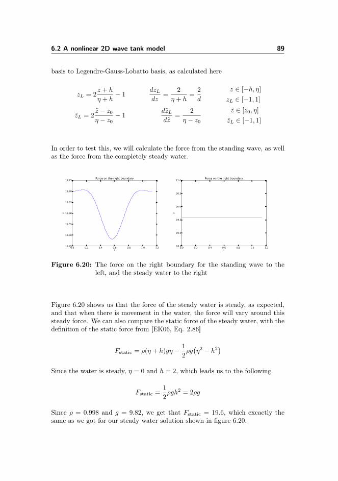
6.2 A nonlinear 2D wave tank model 89
basis to Legendre-Gauss-Lobatto basis, as calculated here
zL = 2z + h
η + h− 1
dzLdz
=2
η + h=
2
d
z ∈ [−h, η]
zL ∈ [−1, 1]
zL = 2z − z0η − z0
− 1dzLdz
=2
η − z0z ∈ [z0, η]
zL ∈ [−1, 1]
In order to test this, we will calculate the force from the standing wave, as wellas the force from the completely steady water.
0.0 0.2 0.4 0.6 0.8 1.0 1.2t
19.45
19.50
19.55
19.60
19.65
19.70
19.75
F
Force on the right boundary
0.0 0.2 0.4 0.6 0.8 1.0 1.2t
18.5
19.0
19.5
20.0
20.5
21.0
F
Force on the right boundary
Figure 6.20: The force on the right boundary for the standing wave to theleft, and the steady water to the right
Figure 6.20 shows us that the force of the steady water is steady, as expected,and that when there is movement in the water, the force will vary around thissteady force. We can also compare the static force of the steady water, with thedefinition of the static force from [EK06, Eq. 2.86]
Fstatic = ρ(η + h)gη − 1
2ρg(η2 − h2
)Since the water is steady, η = 0 and h = 2, which leads us to the following
Fstatic =1
2ρgh2 = 2ρg
Since ρ = 0.998 and g = 9.82, we get that Fstatic = 19.6, which excactly thesame as we got for our steady water solution shown in figure 6.20.
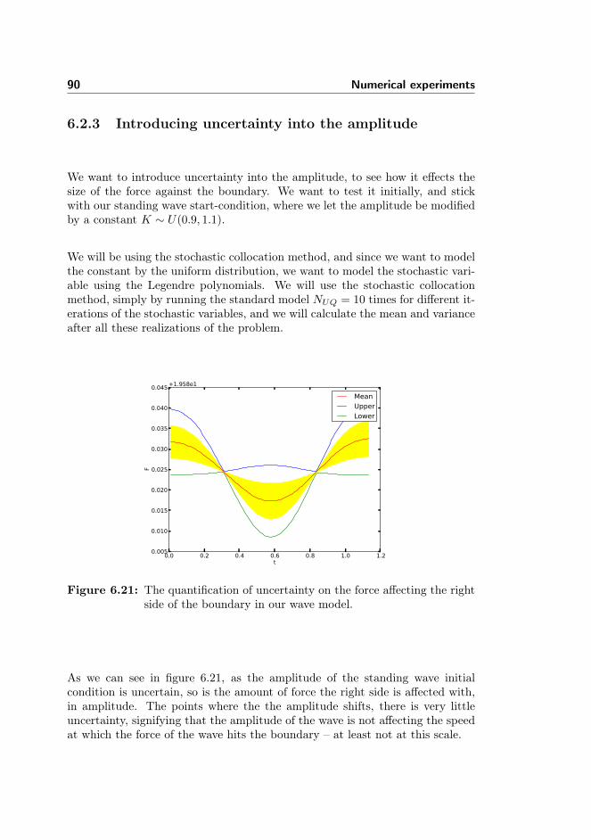
90 Numerical experiments
6.2.3 Introducing uncertainty into the amplitude
We want to introduce uncertainty into the amplitude, to see how it effects thesize of the force against the boundary. We want to test it initially, and stickwith our standing wave start-condition, where we let the amplitude be modifiedby a constant K ∼ U(0.9, 1.1).
We will be using the stochastic collocation method, and since we want to modelthe constant by the uniform distribution, we want to model the stochastic vari-able using the Legendre polynomials. We will use the stochastic collocationmethod, simply by running the standard model NUQ = 10 times for different it-erations of the stochastic variables, and we will calculate the mean and varianceafter all these realizations of the problem.
0.0 0.2 0.4 0.6 0.8 1.0 1.2t
0.005
0.010
0.015
0.020
0.025
0.030
0.035
0.040
0.045
F
+1.958e1
MeanUpperLower
Figure 6.21: The quantification of uncertainty on the force affecting the rightside of the boundary in our wave model.
As we can see in figure 6.21, as the amplitude of the standing wave initialcondition is uncertain, so is the amount of force the right side is affected with,in amplitude. The points where the the amplitude shifts, there is very littleuncertainty, signifying that the amplitude of the wave is not affecting the speedat which the force of the wave hits the boundary – at least not at this scale.

6.2 A nonlinear 2D wave tank model 91
6.2.4 Numerical experiments with uncertainty
For the numerical experiments, we will be using a simple gaussian curve, verymuch like the density function for the gaussian distribution, to emulate a startingwave in our domain.
For this purpose we will be using the function
η0(x) =e
(x−0.01)2
2∗0.082
100(6.30)
Where we will be truncating all values less that e−6, as to simulate a singularwave. We will use this since it confines to our space nicely, and is smooth enoughto approximate correctly.
−1.0 −0.5 0.0 0.5 1.0x
−0.005
0.000
0.005
η
t=0.00
Figure 6.22: The initial condition for our gaussian wave on a grid with Nx =70 and Nz = 25
We will first calculate the solution for this, as to analyze it before introducingthe uncertainty. We simply solve it until t = 1, to briefly evaluate the evolutionof the solution.

92 Numerical experiments
−1.0 −0.5 0.0 0.5 1.0x
−0.005
0.000
0.005
η
t=0.20
−1.0 −0.5 0.0 0.5 1.0x
−0.005
0.000
0.005
η
t=0.60
−1.0 −0.5 0.0 0.5 1.0x
−0.005
0.000
0.005
η
t=0.80
−1.0 −0.5 0.0 0.5 1.0x
−0.005
0.000
0.005
η
t=1.00
Figure 6.23: The evolution of the wave model for the initial condition (6.30)at certain points in time
We see in figure 6.23 that the initial wave collapses into the wave-tank and splitsinto two separate waves, which move towards their respective boundaries.
0.0 0.2 0.4 0.6 0.8 1.0t
9.794
9.796
9.798
9.800
9.802
9.804
9.806
9.808
9.810
F
Force on the right boundary
Nx=70, Ny=25
Figure 6.24: The force on the right boundary wall, exerted by the water.
Figure 6.24 shows us that the force varies as the water moves internally. Wewill be expecting a peak somewhat when the wave we see forming hits the wall.
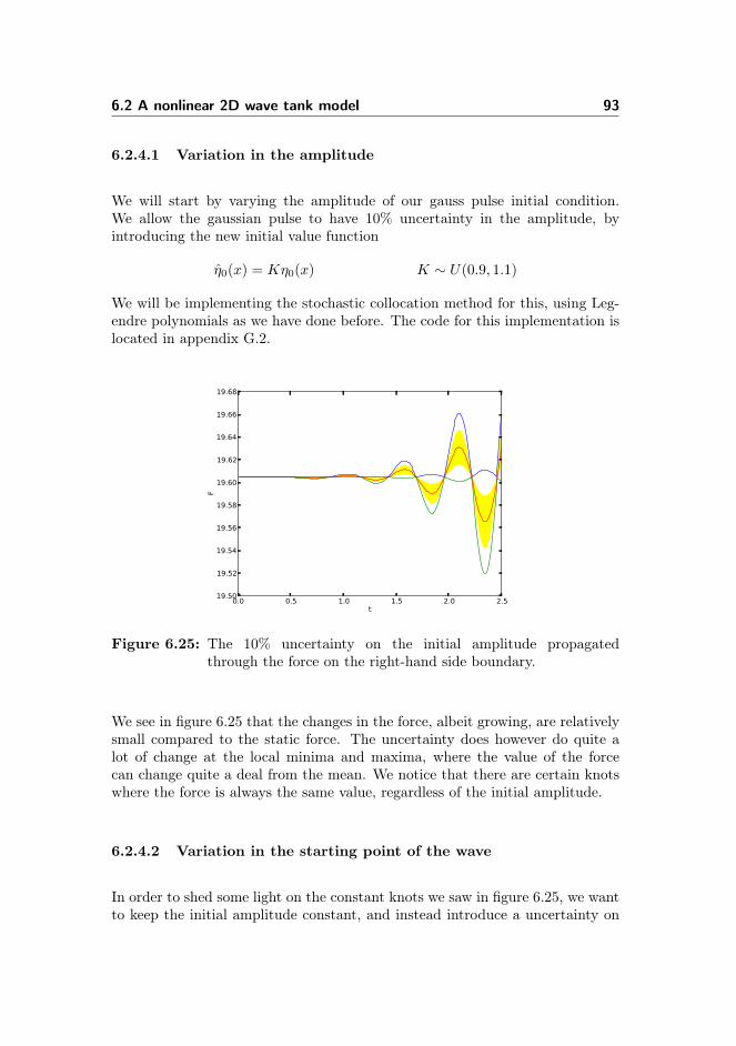
6.2 A nonlinear 2D wave tank model 93
6.2.4.1 Variation in the amplitude
We will start by varying the amplitude of our gauss pulse initial condition.We allow the gaussian pulse to have 10% uncertainty in the amplitude, byintroducing the new initial value function
η0(x) = Kη0(x) K ∼ U(0.9, 1.1)
We will be implementing the stochastic collocation method for this, using Leg-endre polynomials as we have done before. The code for this implementation islocated in appendix G.2.
0.0 0.5 1.0 1.5 2.0 2.5t
19.50
19.52
19.54
19.56
19.58
19.60
19.62
19.64
19.66
19.68
F
Figure 6.25: The 10% uncertainty on the initial amplitude propagatedthrough the force on the right-hand side boundary.
We see in figure 6.25 that the changes in the force, albeit growing, are relativelysmall compared to the static force. The uncertainty does however do quite alot of change at the local minima and maxima, where the value of the forcecan change quite a deal from the mean. We notice that there are certain knotswhere the force is always the same value, regardless of the initial amplitude.
6.2.4.2 Variation in the starting point of the wave
In order to shed some light on the constant knots we saw in figure 6.25, we wantto keep the initial amplitude constant, and instead introduce a uncertainty on

94 Numerical experiments
the midpoint of the wave. We create a new initial value function, from (6.30)
η0(x) =e
(x−ω)2
2∗0.082
100ω ∼ U(−0.02, 0.02)
We use the exact same framework as when we introduced uncertainty to theamplitude, and compute the result
0.0 0.5 1.0 1.5 2.0 2.5t
19.40
19.45
19.50
19.55
19.60
19.65
19.70
19.75
F
MeanUpperLower
Figure 6.26: The uncertainty in the mid-point of our initial pulse ω ∼U(−0.02, 0.02) propagated to the force on the right hand wall.
We see from figure 6.26 that as long as the the starting amplitude is unchanged,the value of the force hitting the wall is close to equal, just either delayed orhurried according to mean. But that is only when the waves are more aligned,which they seem to become at around t = 1.75. Until that, it seems that whereever the pulse starts creates different waves, that hit the wall at different times,allowing those "bubbles" to form on our force plot.
6.2.5 Conclusions for the wave tank model
The wave tank experiment has shown us that the nonlinear systems can packquite a surprise for us, as we have seen in figure 6.26, a small change in the initialcondition can affect the solution in different ways at different times – somethingnot readily apparent from the model itself. This proves that uncertainty quan-tification is a massively useful tool, as it allows us to quantify the effects ofuncertainty we would not be able to understand without this technique. While

6.2 A nonlinear 2D wave tank model 95
this was a relatively heavy model, since each time-step required four solutionsto a Laplace problem on a 70 × 25 grid, it would have been impossible to usethe simple Monte Carlo method to acquire these results.

96 Numerical experiments

Chapter 7
Conclusions
The spectral methods and generalized polynomial chaos methods make for agreat combination when used for quantifying uncertainty through differentialequations. The combination of fast convergence for both types of methodsgrant enormous opportunity for implementation on relatively complex models,as the burden of giant matrix operations become somewhat lessened by havingfewer points.
While the methods are smart, they require a good understanding of the problemto implement properly, and because they work on the whole spectra, it can behard to locate a single error if the methods are not very well understood. Whilebeing more complicated than some easier models, the collocation methods, bothspectral and stochastic merge some good of both worlds, allowing for relativelystraightforward implementation, while retaining the spectral convergence. Withthese two methods, we will be able to do uncertainty quantification on most dif-ferential equation problems relatively easy, while the Galerkin methods requiresomewhat more work per problem.
These methods can of course be paired with other numerical methods or tech-nologies, to increase the speed further, allowing even more applications of thesemethods. One such choice could be to parallelize the processes. With the uncou-pled nature of the stochastic collocation method, many of the processes wouldeasily run in parallel, allowing for fast and efficient calculations, without fear of
98 Conclusions
interdependencies slowing the gain of parallelization.
The applications of uncertainty quantification are everywhere, as it is oftenhard to both measure correctly, and replicate exactly. For some applicationsthis might change the outcome a whole lot, as we saw in burgers equation, orgenerate unanticipated results as we saw in the wave tank model. It might alsojust highlight the inner workings of a model that are not readily apparent fromthe way things work, as we saw in the lid driven cavity model.
Appendix A
Conventions for notationand plotting
A.1 Differential notation
We will be using the following notation for differential notation interchangeably
du(x, t)
dt= ∂tu(x, t) = ut(x, t)
A.2 Uncertainty quantification in plots
We will use two-dimensional plots as a way to visualize the uncertainty quan-tification. We will be using a plot from figure 5.7 to illustrate the point.
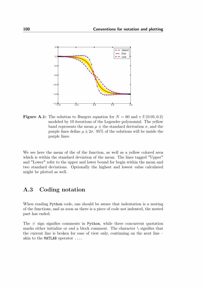
100 Conventions for notation and plotting
−1.0 −0.5 0.0 0.5 1.0−1.5
−1.0
−0.5
0.0
0.5
1.0
1.5
UpperExpLow
Figure A.1: The solution to Burgers equation for N = 60 and v U(0.05, 0.2)modeled by 10 iterations of the Legendre polynomial. The yellowband represents the mean µ ± the standard derivation σ, and thepurple lines define µ± 2σ. 95% of the solutions will be inside thepurple lines.
We see here the mean of the of the function, as well as a yellow colored areawhich is within the standard deviation of the mean. The lines tagged "Upper"and "Lower" refer to the upper and lower bound for begin within the mean andtwo standard deviations. Optionally the highest and lowest value calculatedmight be plotted as well.
A.3 Coding notation
When reading Python code, one should be aware that indentation is a nestingof the functions, and as soon as there is a piece of code not indented, the nestedpart has ended.
The # sign signifies comments in Python, while three concurrent quotationmarks either initialize or end a block comment. The character \ signifies thatthe current line is broken for ease of view only, continuing on the next line –akin to the MATLAB operator ....

Appendix B
Allan P. Engsig-Karup,notes

102 Allan P. Engsig-Karup, notes
Figure B.1: Origin of Lambda A.1

Appendix C
Code used in chapter 3
C.1 Generating plots
Lagrange polynomials
1 # -*- coding: utf-8 -*-2 """3 Created on Tue Jan 22 15:20:30 20134
5 @author: cbrams6
7 This function is simply showing the lagrance polynomials for N=68 """9 import numpy as np
10 import matplotlib.pyplot as plt11
12 N = 613 i = np.array(range(N+1))14 xj = np.zeros((len(i)))15
16 #Calculate the points

104 Code used in chapter 3
17 for j in i:18 xj[j] = 2.*np.pi/float(N)*j19
20 #Create a fine grid to plot on21 x = np.linspace(xj[0]-1e-12,xj[N]+1e-12,100)22
23 #Plot the Lagrange polynomials24 for j in i:25 hj = 1./float(N) * np.sin(N/2. *(x-xj[j])) * np.cos(1./2.*(x-xj[j])) / np.sin(1./2.*(x-xj[j]))26 hj[np.isnan(hj)] = 0.27 plt.plot(x/(2.*np.pi),hj)28 plt.grid()29 plt.xlim(0.,1)30 plt.title("Lagrange polynomials for N=%d"%N)31 plt.savefig("../../Latex/Billeder/Chapter3/LagrangePolynomials.eps")
Legendre polynomials
1 # -*- coding: utf-8 -*-2 """3 Created on Tue Jan 22 15:20:30 20134
5 @author: cbrams6
7 This script is intended to show the Legendre polynomials8 """9
10 #Initilization11 import numpy as np12 import DABISpectral1D13 import matplotlib.pyplot as plt14
15 #Generate x-points16 x = np.linspace(-1,1,100)17 for N in range(6):18
19 #Initialize Legendre polynomial, and calculate values20 # (0.0,0.0) is (alpha, beta)21 polyLeg = DABISpectral1D.Poly1D(DABISpectral1D.JACOBI,(0.0,0.0))22 p5Leg = polyLeg.GradEvaluate(x, N, 0); # N is N23
24 #Plot polynomials
C.1 Generating plots 105
25 plt.plot(x,p5Leg,label=’N = ’+str(N))26 plt.legend()27 plt.title(’Legendre polynomials’)28 plt.savefig("../../Latex/Billeder/Chapter3/LegendrePolynomials.eps")
Gibbs phenomenon
1 # -*- coding: utf-8 -*-2 """3 Created on Sun Jan 20 11:38:19 20134
5 @author: cbrams6
7 This script is intended to show Gibbs phenomenon8 """9 import numpy as np
10 import DABISpectral1D as DB11 import matplotlib.pyplot as plt12
13 #Define the step-function14 def f(x):15 F = np.zeros(x.shape)16 F[x>0] = 117 F[x<0] = -118 return F19
20 #Plot the step-function21 plt.figure(1)22 xi = np.linspace(-1,1,num=1000)23 plt.plot(xi,f(xi),label="Original")24
25 #Initialize polynomial26 LegPol = DB.Poly1D(DB.JACOBI,(0.0,0.0))27
28 #Increasing N and room for error29 N = np.array([5,15,25,35])30 Err = np.zeros(N.shape)31 for i in range(N.size):32 #Approximate the step function using nodal values33 n = N[i]34 x,w = LegPol.GaussLobattoQuadrature(n)35 F = f(x)

106 Code used in chapter 3
36
37 #Calculate modal coefficients and interpolation38 fhat = LegPol.DiscretePolynomialTransform(x,F,n)39 fi = LegPol.LagrangeInterpolate(x,F,xi)40
41 #Plot the coefficients42 plt.figure(1)43 plt.plot(xi,fi,label="N=%d"%n)44 plt.figure(2)45 plt.semilogy(range(n+1),fhat,’o’,label="N=%d"%n)46 Err[i] = max(abs(fi-f(xi)))47
48 #Plot the results49 plt.figure(1)50 plt.legend(loc=4)51 plt.savefig("../../Latex/Billeder/Chapter3/GibbsPhenomenon.eps")52 plt.figure(2)53 plt.legend(loc=6)54 plt.savefig("../../Latex/Billeder/Chapter3/GibbsCoefficients.eps")55 plt.figure(3)56 plt.semilogy(range(N.size),Err)57 plt.title("Error")58 plt.show()
Aliasing
1 # -*- coding: utf-8 -*-2 """3 Created on Sun Jan 20 13:03:12 20134
5 @author: cbrams6
7 This script is intended to illustrate the aliasing problem8 """9 import numpy as np
10 import matplotlib.pyplot as plt11
12 #Calculate the arrays13 x = np.linspace(0,2*np.pi,1000)14 X = np.linspace(0,2*np.pi,9,endpoint=True)15
16 #Calculate the complex exponentials
C.1 Generating plots 107
17 z2 = 1j*2*x18 z6 = 1j*-6*x19 Z = 1j*2*X20 E2 = np.exp(z2)21 E6 = np.exp(z6)22 E = np.exp(Z)23
24 #Plot it all together25 plt.figure()26 plt.plot(x,np.real(E2),label="k=2",linestyle="--")27 plt.plot(x,np.real(E6),label="k=-6",linestyle="--")28 plt.plot(X,np.real(E),’o’)29 plt.xlim(0-0.02,2*np.pi+0.02)30 plt.ylim(-1.02,1.02)31 plt.legend()32 plt.savefig("../../Latex/Billeder/Chapter3/Aliasing.eps")

108 Code used in chapter 3
Appendix D
Code used in chapter 4
D.1 Differential Matrices
The Diff function
1 # -*- coding: utf-8 -*-2 """3 Created on Wed Jan 2 19:52:09 20134
5 @author: cbrams6
7 This script is intended to calculate the differential operators8 """9
10 #Initilization11 import numpy as np12 import DABISpectral1D as DB13
14 #Function generating differentiative matrix15 def DF(N):16 D = np.zeros((N,N))
110 Code used in chapter 4
17 #Generate for even N18 if (N%2)==0:19 for l in range(N):20 for k in range(N):21 if l==k:22 D[k][l] = 023 else:24 D[k][l] = (1/2.)*(-1)**(1+k+l)\25 *np.cos(np.pi*(-k+l)/N)/np.sin(np.pi*(-k+l)/N)26 else:27 D = 028 return D29
30 def DP(N):31 #Initialize Polynomial32 P = DB.Poly1D(DB.JACOBI, (0.0,0.0))33
34 #Generate grid35 (xGL,w) = P.GaussLobattoQuadrature(N-1)36
37 #Generate Vandermonde Matrices38 V = P.GradVandermonde1D(xGL,N-1,0)39 Vx = P.GradVandermonde1D(xGL,N-1,1)40
41 #Solve for D42 D = np.linalg.solve(V.T,Vx.T).T43 return [D,xGL]
D.2 Test functions
The test for the Fourier differential operator
1 # -*- coding: utf-8 -*-2 """3 Created on Wed Jan 2 19:54:08 20134
5 @author: cbrams6
7 This script is intended to test the fourier differentiation8 operator
D.2 Test functions 111
9 """10
11 #Initilization12 from __future__ import division13 from Diff import DF14 import numpy as np15
16 #Setting number of N values evaluated17 Niter = 1518 error = np.zeros(Niter)19
20 for i in range(Niter):21 #Initiliza loop22 N = 4*i+523 x = np.linspace(0,2,N)24
25 #Generating true values26 dv = np.cos(np.pi*x)*np.pi*np.exp(np.sin(np.pi*x))27 v = np.exp(np.sin(np.pi*x))28
29 #Differentiating using D30 Dv = np.zeros(v.shape)31 Dv[0:N-1] = np.dot(DF(N-1),v[0:N-1])*np.pi32 Dv[N-1] = Dv[0]33 error[i] = max(abs(dv-Dv))34
35
36 #Plotting approximation37 import matplotlib.pyplot as plt38 plt.figure()39 plt.plot(x,dv,label=’Analytic’,color=’b’)40 plt.plot(x,Dv,linestyle=’ ’,marker=’x’,color = ’r’,\41 label=’Approximation’)42 plt.xlabel("x")43 plt.ylabel("v’(x)")44 plt.legend()45 plt.savefig("../../Latex/Billeder/Chapter4/FourierDTestResult.eps")46
47
48 #Plotting error49 plt.figure()50 NN = 4*np.array(range(Niter))+551 plt.loglog(NN,error,’r’,label=’Error’)52 plt.loglog(NN,1/NN**(3),’b’,label=’N^(-3)’)
112 Code used in chapter 4
53 plt.xlabel("N")54 plt.legend()55 plt.savefig("../../Latex/Billeder/Chapter4/FourierDTestConvergence.eps")56
57 #Show plots58 #plt.show()
The test for the Legendre differential operator
1 # -*- coding: utf-8 -*-2 """3 Created on Thu Jan 3 14:01:08 20134
5 @author: cbrams6
7 This script is intended to test the LEgendre differential operator8 """9 #Initialization
10 from numpy import pi,sin,exp,cos11 import numpy as np12 import DABISpectral1D as DB13 from numpy.linalg import norm14 import matplotlib.pyplot as plt15 from Diff import DP16
17 #Correct value functions18 v = lambda x: exp(sin(pi*x))19 dv = lambda x: pi*cos(pi*x)*exp(sin(pi*x))20
21 #Initialize polynomials22 P = DB.Poly1D(DB.JACOBI, (0.0,0.0))23
24 #Initialize loop over N25 nn = 526 error = np.zeros(nn)27 for i in range(nn):28 N = 2**(i+2)29
30 #Generate D and x31 [D,xGL] = DP(N)32 x = xGL + 133

D.2 Test functions 113
34 #Calculate function values35 f = v(x)36
37 #Calculate approximated and analytic function values38 df = np.dot(D,f)39 Df = dv(x)40
41 #Record error42 error[i] = norm(df-Df,2)43
44 plt.figure()45 plt.plot(x,Df,label=’Analytic’,color=’b’)46 plt.plot(x,df,linestyle=’ ’,marker=’x’,color = ’r’,\47 label=’Approximation’)48 plt.xlabel("x")49 plt.ylabel("v’(x)")50 plt.legend()51 plt.savefig("../../Latex/Billeder/Chapter4/LegendreDTestResult.eps")52
53
54 #Print error55 plt.figure()56 NN = (np.ones(nn)*2)**(np.array(range(nn))+1)57 plt.loglog(NN,error,label="Error")58 plt.loglog(NN,NN**(-2),label="N^(-2)")59 plt.xlabel("N")60 plt.legend()61 plt.savefig("../../Latex/Billeder/Chapter4/LegendreDTestConvergence.eps")
D.2.1 The test for the two-dimensional differential
1 # -*- coding: utf-8 -*-2 """3 Created on Wed Jan 23 16:42:52 20134
5 @author: cbrams6
7 This is intended for creating a plot showing the effectiveness8 of the differential operators.9 """
10
11 from __future__ import division
114 Code used in chapter 4
12 import numpy as np13 import DABISpectral1D as DB14 from Diff import DP15 import matplotlib.pyplot as plt16
17 N = 2018
19 LegPol = DB.Poly1D(DB.JACOBI,(0.0,0.0))20
21 #Generate the mesh22 x,wx = LegPol.GaussLobattoQuadrature(N)23 y,wy = LegPol.GaussLobattoQuadrature(N)24
25 X,Y = np.meshgrid(x,y)26
27 #Calculate the initial and true value28 C = np.cos(X*Y)29 Cprime = -np.cos(X*Y)*X*Y-np.sin(X*Y)30
31 #Generate the matrices32 [Dx,_] = DP(N+1)33 [Dy,_] = DP(N+1)34
35 #Creating the matrices for multidimensional use36 DX = np.kron(Dx,np.identity(N+1))37 DY = np.kron(np.identity(N+1),Dy)38
39 #Flattening the initial condition40 C = C.flatten("F")41
42 #Calculating the derivative and reshaping43 Cd = np.dot(DX,np.dot(DY,C))44 Cd = Cd.reshape([N+1,N+1],order="F")45
46 #Plotting47 plt.figure()48 plt.imshow(np.abs(Cd-Cprime),origin="lower",extent=[-1,1,-1,1])49 plt.colorbar()50 plt.xlabel(’x’)51 plt.ylabel(’y’)52 plt.axis(’normal’)53 plt.savefig("../../Latex/Billeder/Chapter4/MultiDimDiffTest.eps")

D.2 Test functions 115
D.2.2 The test for the sparse matrices speed
1 # -*- coding: utf-8 -*-2 """3 Created on Thu Jan 24 12:29:22 20134
5 @author: cbrams6
7 This is intended to test the sparse matrix dot product speed8 """9
10 import time11 import numpy as np12 from scipy.sparse import lil_matrix13 from numpy.random import rand14
15 #We’re running the scheme 1000 times16 tN = 100017 timeSparse = np.zeros(tN)18 timeFull = np.zeros(tN)19 errors = np.zeros(tN)20 for i in range(tN):21 #Creating and populating the matrix22 A = lil_matrix((1000, 1000))23 A[0, :100] = rand(100)24 A[1, 100:200] = A[0, :100]25 A.setdiag(rand(1000))26
27 #Transforming the matrix28 A = A.tocsr()29 b = rand(1000)30
31 #Time the Dense product as well32 AA = A.todense()33 T1 = time.clock()34 x = A.dot(b)35 T2 = time.clock()36 y = np.dot(AA,b)37 T3 = time.clock()38
39 #Calculate the error between the two solutions40 errors[i] = np.linalg.norm(x**2-np.array(y)**2,ord=2)41

116 Code used in chapter 4
42 #Storing the time43 timeSparse[i] = T2-T144 timeFull[i] = T3-T245
46 #Calculate and print the averages47 TS = np.average(timeSparse)48 TF = np.average(timeFull)49 E = np.average(errors)50
51 print TS52 print TF53 print E
D.3 Practical implementations
The test script for the boundary value problem
1 # -*- coding: utf-8 -*-2 """3 Created on Thu Jan 24 15:48:05 20134
5 @author: cbrams6
7 This script is intended to solve the problem with BVP presented8 in the spectral chapter9 """
10 #Initialization11 import numpy as np12 from numpy.linalg import norm13 import DABISpectral1D14 import matplotlib.pyplot as plt15 from Diff import DP16 plt.close(’all’)17
18 #Generate iteration parameters19 N = np.linspace(10,80,num=71)20
21 epsilon = 0.0122 error = np.zeros([len(N)])23 for i in range(len(N)):

D.3 Practical implementations 117
24 n = int(N[i] )25 b = -126
27 #Initialize polynomial28 polyLeg = DABISpectral1D.Poly1D(DABISpectral1D.JACOBI, (0.0,0.0))29
30 #Generate Quadrature and transformation31 [D,y] = DP(n)32 x = (y+1)/233
34 #Construct L35 L = -epsilon*4*np.dot(D,D) + b*2*D36
37 #Implement boundary conditions38 L[0,:] = 039 L[-1,:] = 040 L[0,0] = 141 L[-1,-1] = 142
43 #Generate right-side function with boundary conditions44 f = np.ones((n,1))45 f[0] = 046 f[-1] = 047
48 #Solve system and calculate exact solution49 u = np.linalg.solve(L,f)50 uExact = (np.exp((1-x)/epsilon)+np.exp(1/epsilon)*\51 (x-1)-x)/(1-np.exp(1/epsilon))52
53 #Calculate error54 error[i] = norm(u[:,0]-uExact,np.inf)55
56 #Plot function57 plt.figure()58 plt.plot(x,u,’ro’,label="Approximation")59 plt.plot(x,uExact,label="Exact")60 plt.xlabel("x")61 plt.title("N=" + str(n) + " and epsilon="+str(epsilon))62 plt.legend()63 plt.savefig("../../Latex/Billeder/Chapter4/EpsilonSolution.eps")64
65
66 #Errorplot67 plt.figure()
118 Code used in chapter 4
68 plt.loglog(N,error[:],’r’,label="Error \epsilon="+str(epsilon))69 plt.legend()70 plt.xlabel("N")71 plt.savefig("../../Latex/Billeder/Chapter4/EpsilonError.eps")
The test script for Burgers’ equation
1 # -*- coding: utf-8 -*-2 """3 Created on Mon Jan 21 20:05:23 20134
5 @author: cbrams6
7 This script is intended to solve Burger’s problem with a8 pseudo-spectral method9 """
10
11 from __future__ import division12 import numpy as np13 import matplotlib.pyplot as plt14 from Diff import DP15 from scipy.integrate import odeint16
17
18 def initialValue(x):19 #Calculate initial value20 res = -np.tanh((x))21 #Adjust boundaries22 res = res/np.abs(res[0])23 return res24
25 def dudt(u,t,v,Dx,BoundaryFixer):26 #Calculating linear operator27 unew= -u*np.dot(Dx,u)+v*np.dot(Dx,np.dot(Dx,u))28 #Adjust for boundaries29 unew = unew*BoundaryFixer30 return unew31
32
33 #Initialization34 xN = 8035 v = 0.1
D.3 Practical implementations 119
36
37
38 #Generating Dx and u039 Dx,x = DP(xN)40 u0 = initialValue(x)41
42 #Configuring time needed43 tEnd = 444 tNum = 100045 #We create the time-array we want values for46 t = np.linspace(0,tEnd,tNum)47
48 #Create boundary fixer to cancel the time derivatives49 # at the boundaries.50 BDFix = np.ones(x.shape)51 BDFix[0] = 052 BDFix[-1] = 053
54 #Start the time-integrator55 v0 = v56 usol = odeint(dudt,u0,t,tuple([v0,Dx,BDFix]))57
58 #Plot the solutions59 plt.figure()60 plt.title("Solution to Burgers’ equation")61 plt.plot(x,initialValue(x),’r--’,linewidth=2,label="Initial Value")62 for i in range(1,6):63 plt.plot(x,usol[i*100,:],label="t=%.2f"%t[i*100])64 plt.plot(x,usol[-1,:],label="t=%2d"%t[-1])65 plt.xlabel("x")66 plt.ylim(-1.1,1.1)67 plt.legend()68
69 plt.savefig("../../Latex/Billeder/Chapter4/BurgersEQSpectral.eps")

120 Code used in chapter 4
Appendix E
Code used in chapter 5
E.1 Visualization
Visualising the first six Hermite polynomials
1 # -*- coding: utf-8 -*-2 """3 Created on Sat Jan 12 10:39:12 20134
5 @author: cbrams6
7 This script is intended for showing the hermite polynomials8 """9
10 import DABISpectral1D as DB11 import numpy as np12 import matplotlib.pyplot as plt13
14 #Initialize Polynomial15 HPol = DB.Poly1D(’HermitePprob’,())16
122 Code used in chapter 5
17 #Generate grid18 xlim = 319 N = 10020 x = np.linspace(-xlim,xlim,N)21
22 plt.figure()23 for i in range(6):24 #Evaluate and plot polynomials25 polyval = HPol.GradEvaluate(x,i,0)26 plt.plot(x,polyval,label="HP"+str(i))27
28 plt.legend(loc=9)29 plt.savefig("../../Latex/Billeder/Chapter5/HermitePolynomials.eps")
E.2 Practical examples
E.2.1 Test equation
Monte Carlo mean approximation
1 # -*- coding: utf-8 -*-2 """3 Created on Thu Jan 10 12:52:18 20134
5 @author: cbrams6
7 This script is designed for calculating the mean by the8 Monte Carlo methods9 """
10 #Imports11 from __future__ import division12 import numpy as np13 from scipy.integrate import odeint14 from numpy.random import normal as alpha15 from math import e16 import matplotlib.pyplot as plt17
18
19 #Define time-derivative for one random parameter20 def dudt(u,t,args):
E.2 Practical examples 123
21 return -args*u22
23 #True solution24 def u(t,mean,std):25 a = alpha(mean,std)26 return e**(-a*t),a27
28 #Define mean, standard deviation and expectation29 mean = 9.30 std = 3.31 tTrue = 0.532 TrueExp = e**(1/2*tTrue**2*std**2-tTrue*mean)33
34 tN = 10035 t = np.linspace(0,tTrue,tN)36
37
38 #Number of realizations39 M = 10000040
41 NSol = np.zeros(M)42 NRunningMean = np.zeros(M)43 NRunningVar = np.zeros(M)44 for N in range(M):45 #Calculate a random starting point46 y0,a = u(0,mean,std)47
48 #Integrate over time49 sol = odeint(dudt,y0,t,tuple([a]))50
51 #Calculate the running mean52 NSol[N] = sol[-1]53 NRunningMean[N] = np.mean(NSol[:N])54
55 plt.figure()56 plt.plot(range(M),NRunningMean,label="Running Mean");57 plt.plot(range(M),np.ones(M)*TrueExp,label="Expectation")58 plt.xlabel("N")59 plt.legend()60 plt.savefig("../../Latex/Billeder/Chapter5/TestEQMonteCarloRunningMean.eps")61
62 plt.figure()63 plt.loglog(range(M),abs(NRunningMean-TrueExp),label="Error");64 plt.xlabel("N")

124 Code used in chapter 5
65 plt.legend()66 plt.savefig("../../Latex/Billeder/Chapter5/TestEQMonteCarloRunningError.eps")
Collocation mean and variance approximation
1 # -*- coding: utf-8 -*-2 """3 Created on Fri Jan 11 12:46:31 20134
5 @author: cbrams6
7 This script is intended to calculate the mean and variance8 for the test equation by the spectral collocation method9 """
10 from __future__ import division11 import DABISpectral1D as DB12 import numpy as np13 from math import e14 from scipy.integrate import odeint15 import matplotlib.pyplot as plt16
17 #True solution18 def u(t,a):19 return e**(-a*t)20
21 def dudt(u,t,a):22 return -a*u23 #Initialize Polynomial24 HPol = DB.Poly1D(’HermitePprob’,())25
26 #Set number of time steps, as well as calculating the real values27 tN = 100028 mean = 929 std = 330 tTrue = 0.531 TrueExp = e**(1/2*tTrue**2*std**2-tTrue*mean)32 TrueVar = (e**(tTrue**2*std**2)-1)*\33 e**(-2*tTrue*mean+tTrue**2*std**2)34
35 t = np.linspace(0,tTrue,tN)36
37 NMax = 25

E.2 Practical examples 125
38 Exp = np.zeros(NMax-1)39 ExpVar = np.zeros(NMax-1)40 for N in range(1,NMax):41 #Generate points42 x,w = HPol.GaussQuadrature(N)43
44 #Generate the random variable representation45 a = mean + (std)*x;46
47 #Fint initial value48 u0 = u(0,a)49
50 #Integrate over time51 sol = odeint(dudt,u0,t,tuple([a]))52 ufinal = sol[-1]53
54 #Calculate Expectation and variance55 Exp[N-1] = sum(w[:,0]*ufinal)56 ExpVar[N-1] = sum(w[:,0]*((ufinal-Exp[N-1]))**2)57
58 plt.figure59 NN = np.array(range(1,NMax))60 plt.plot(NN,Exp,label="Approximated exp")61 plt.plot(NN,np.ones(NMax-1)*TrueExp,label="True exp")62 plt.xlabel("N")63 plt.legend()64
65 NN = np.array(range(1,NMax))66 plt.plot(NN,ExpVar,label="Approximated variance")67 plt.plot(NN,np.ones(NMax-1)*TrueVar,label="True variance")68 plt.xlabel("N")69 plt.legend()70 plt.savefig("../../Latex/Billeder/Chapter5/TestEQCollocationMean.eps")71
72 plt.figure()73 plt.semilogy(NN,abs(Exp-TrueExp),label="Error mean")74 plt.semilogy(NN,abs(ExpVar-TrueVar),label="Error Variance")75 plt.xlabel("N")76 plt.title("Absolute error")77 plt.legend()78 plt.savefig("../../Latex/Billeder/Chapter5/TestEQCollocationError.eps")79 plt.show()80
81 np.savez("test",Exp=Exp,ufinal=ufinal)
126 Code used in chapter 5
Monte Carlo mean approximation for the uniform case
1 # -*- coding: utf-8 -*-2 """3 Created on Mon Jan 21 10:45:51 20134
5 @author: cbrams6
7 This script is intended to calculate the Monte Carlo mean8 for a uniform distribution9 """
10
11 #Imports12 from __future__ import division13 import numpy as np14 from scipy.integrate import odeint15 from numpy.random import uniform as alpha16 from math import e17 import matplotlib.pyplot as plt18
19
20 #Define time-derivative for once random parameter21 def dudt(u,t,args):22 return -args*u23
24 #True solution25 def u(t,start,end):26 a = alpha(low=start,high=end)27 return e**(-a*t),a28
29 #Define mean, standard deviation and expectation30 start = -731 end = 232 tTrue = 0.533 TrueExp = (-e**(-start*tTrue)+e**(-end*tTrue))/(tTrue*(start-end))34
35 tN = 10036 t = np.linspace(0,tTrue,tN)37
38
39 #Number of realizations40 M = 10000041
E.2 Practical examples 127
42 NSol = np.zeros(M)43 NRunningMean = np.zeros(M)44 for N in range(M):45 #Generate random start46 y0,a = u(0,start,end)47
48 #Integrate over time49 sol = odeint(dudt,y0,t,tuple([a]))50
51 #Calculate running mean52 NSol[N] = sol[-1]53 NRunningMean[N] = np.mean(NSol[:N])54
55 plt.figure()56 plt.plot(range(M),NRunningMean,label="Running Mean");57 plt.plot(range(M),np.ones(M)*TrueExp,label="Expectation")58 plt.xlabel("N")59 plt.legend()60 plt.savefig("../../Latex/Billeder/Chapter5/TestEQMonteCarloRunningMeanUniform.eps")61
62 plt.figure()63 plt.loglog(range(M),abs(NRunningMean-TrueExp),label="Error");64 plt.xlabel("N")65 plt.legend()66 plt.savefig("../../Latex/Billeder/Chapter5/TestEQMonteCarloRunningErrorUniform.eps")
Collocation mean approximation for the uniform case
1 # -*- coding: utf-8 -*-2 """3 Created on Sat Jan 12 10:58:40 20134
5 @author: cbrams6 """7 from __future__ import division8 import DABISpectral1D as DB9 import numpy as np
10 from math import e11 from scipy.integrate import odeint12 import matplotlib.pyplot as plt13
14 #True solution
128 Code used in chapter 5
15 def u(t,a):16 return e**(-a*t)17
18 def dudt(u,t,a):19 return -a*u20 #Initialize Polynomial21 JPol = DB.Poly1D(’Jacobi’,(0.0,0.0))22
23
24 start = -725 end = 226 tTrue = 0.527 TrueExp = (-e**(-start*tTrue)+e**(-end*tTrue))/(tTrue*(start-end))28
29 t = np.linspace(0,tTrue,2)30
31 NMax = 2532 Exp = np.zeros(NMax-1)33 ExpVar = np.zeros(NMax-1)34 for N in range(1,NMax):35 #Generate points36 x,w = JPol.GaussQuadrature(N)37
38 #Generate random representation39 x = (x+1)/2*(end-start)+start40
41 a = x42 a[x>end] = 043 a[x<start] = 044
45
46 #Solve for time47 u0 = u(0,a)48 sol = odeint(dudt,u0,t,tuple([a]))49
50 #Employ correct weights51 w = w/252 Exp[N-1] = sum(w[:,0]*sol[-1])53 ExpVar[N-1] = sum(w[:,0]*sol[-1]**2)54
55 plt.figure56 NN = np.array(range(1,NMax))57 plt.plot(NN,Exp,label="Approximated exp")58 plt.plot(NN,np.ones(NMax-1)*TrueExp,label="True exp")

E.2 Practical examples 129
59 plt.xlabel("N")60 plt.legend()61 plt.savefig("../../Latex/Billeder/Chapter5/TestEQCollocationMeanUniform.eps")62
63 plt.figure()64 plt.semilogy(NN,abs(Exp-TrueExp),label="Error")65 plt.xlabel("N")66 plt.title("Absolute error")67 plt.savefig("../../Latex/Billeder/Chapter5/TestEQCollocationMeanErrorUniform.eps")
Stochastic Galerkin method for the mean approximation
1 # -*- coding: utf-8 -*-2 """3 Created on Mon Jan 21 10:33:56 20134
5 @author: cbrams6 """7 from __future__ import division8 import DABISpectral1D as DB9 import numpy as np
10 from math import e11 from scipy.integrate import odeint12 import matplotlib.pyplot as plt13 from scipy.misc import factorial14
15 #True solution16 def u(t,a):17 return e**(-a*t)18
19 def dudt(u,t,A):20 return np.dot(A.T,u)21
22 #Calculate eijk23 def ef(i,j,k,N):24 M = int(np.ceil(3/2*N))25 ePol = DB.Poly1D(’HermitePprob’,())26 z,wz = ePol.GaussQuadrature(M)27
28 Hi = ePol.GradEvaluate(z,i,0)29 Hj = ePol.GradEvaluate(z,j,0)30 Hk = ePol.GradEvaluate(z,k,0)

130 Code used in chapter 5
31
32 E = sum(Hi*Hj*Hk*wz)33
34 return E35 #Initialize Polynomial36 HPol = DB.Poly1D(’HermitePprob’,())37
38 #Initialize computational parameters39 tN = 100040 mean = 941 std = 342 tTrue = 0.543 TrueExp = e**(1/2*tTrue**2*std**2-tTrue*mean)44 t = np.linspace(0,tTrue,tN)45
46 NMax = 3047 Exp = np.zeros(NMax-1)48 for N in range(NMax):49 #Generate points50 x,w = HPol.GaussQuadrature(N)51
52 #Generate representation53 a = mean + (std)*x;54
55 #Transforming56 u0 = u(0,a)57 v0 = HPol.DiscretePolynomialTransform(x,u0,N)58
59 #Generating the A matrix60 A = np.zeros([N+1,N+1])61 for j in range(N+1):62 for k in range(N+1):63 A[j,k] = -1/factorial(k)*(mean*ef(0,j,k,N)+std*ef(1,j,k,N))64
65 #Solve for time66 sol = odeint(dudt,v0,t,tuple([A]))67
68 #Inversely transform69 ufinal = HPol.InverseDiscretePolynomialTransform(x,sol[-1],N)70
71
72 #Calculating expectancy73 Exp[N-1] = sum(w[:,0]*ufinal)74

E.2 Practical examples 131
75 plt.figure76 NN = np.array(range(1,NMax))77 plt.plot(NN,Exp,label="Approximated exp")78 plt.plot(NN,np.ones(NMax-1)*TrueExp,label="True exp")79 plt.xlabel("N")80 plt.legend()81 plt.savefig("../../Latex/Billeder/Chapter5/TestEQGalerkinMean.eps")82
83
84 plt.figure()85 plt.semilogy(NN,abs(Exp-TrueExp),label="Error")86 plt.xlabel("N")87 plt.title("Absolute error")88 plt.savefig("../../Latex/Billeder/Chapter5/TestEQGalerkinError.eps")
Two dimensional stochastic collocation method for the mean approx-imation
1 # -*- coding: utf-8 -*-2 """3 Created on Sun Jan 20 16:52:00 20134
5 @author: cbrams6 """7
8 from __future__ import division9 import DABISpectral1D as DB
10 import numpy as np11 from math import e12 from scipy.integrate import odeint13 import matplotlib.pyplot as plt14
15 #True solution16 def u(t,a,b):17 return b*e**(-a*t)18
19 def dudt(u,t,a):20 return -a*u21 #Initialize Polynomial22 HPol = DB.Poly1D(’HermitePprob’,())23
24

132 Code used in chapter 5
25 #Generate both gaussian distribution coefficients26 tN = 100027 mean = 428 std = 1.529
30 meanB = 331 stdB = 0.1532
33 #Calculate true expectancy34 tTrue = 0.535 TrueExp = meanB*e**(1/2*tTrue**2*std**2-tTrue*mean)36
37 t = np.linspace(0,tTrue,tN)38
39 NMax = 2540 Exp = np.zeros(NMax-1)41 ExpVar = np.zeros(NMax-1)42 for N in range(1,NMax):43 #Generate points44 x,xw = HPol.GaussQuadrature(N)45 y,yw = HPol.GaussQuadrature(N)46
47 #Calculate both stochastic representations48 a = mean + (std)*x;49 b = meanB+stdB*y50
51 #Create a mesh of both stochastic variables and weights52 A,B = np.meshgrid(a,b)53 XW,YW = np.meshgrid(xw,yw)54 W = XW*YW55 W = W.reshape([(N+1)*(N+1)])56
57 #Calculate starting conditions58 V = HPol.GradVandermonde1D(x,N,0)59 u0 = u(0,A,B)60
61 #Reshape solution62 u0 = u0.reshape([(N+1)*(N+1)])63 A = A.reshape([(N+1)*(N+1)])64
65 #Integrate over time66 sol = odeint(dudt,u0,t,tuple([A]))67 ufinal = sol[-1]68

E.2 Practical examples 133
69 #Calculate mean and expectancy70 Exp[N-1] = sum(W*ufinal)71 ExpVar[N-1] = sum(W*ufinal**2)72
73 ExpRunning = np.sum(np.tile(W,[tN,1])*sol,1)74 test = np.tile(ExpRunning,[(N+1)*(N+1),1]).T75
76 VarRunning = np.sum(np.tile(W,[tN,1])*(sol-test)**2,1)77 plt.figure78 NN = np.array(range(1,NMax))79 plt.plot(NN,Exp,label="Approximated exp")80 plt.plot(NN,np.ones(NMax-1)*TrueExp,label="True exp")81 plt.xlabel("N")82 plt.legend()83 plt.savefig("../../Latex/Billeder/Chapter5/TestEq2DGPCApproxExp.eps")84
85 plt.figure()86 plt.semilogy(NN,abs(Exp-TrueExp),label="Error")87 plt.xlabel("N")88 plt.title("Absolute error")89 plt.savefig("../../Latex/Billeder/Chapter5/TestEq2DGPCError.eps")90
91 plt.figure()92 plt.fill_between(t,ExpRunning-np.sqrt(VarRunning),ExpRunning+np.sqrt(VarRunning),color="yellow")93 plt.plot(t,ExpRunning+2*np.sqrt(VarRunning),’r’,label="Upper")94 plt.plot(t,ExpRunning,label="Mean")95 plt.plot(t,ExpRunning-2*np.sqrt(VarRunning),’r’,label="Lower")96 plt.xlabel("t")97 plt.legend()98 plt.savefig("../../Latex/Billeder/Chapter5/TestEq2DGPCSolution.eps")99 plt.show()
E.2.2 Burgers’ equation
Solution to Burgers’ with uncertainty on v
1 # -*- coding: utf-8 -*-2 """3 Created on Sat Jan 12 17:44:27 20134
5 @author: cbrams
134 Code used in chapter 5
6 """7
8 from __future__ import division9 import numpy as np
10 import DABISpectral1D as DB11 import matplotlib.pyplot as plt12 from Diff import DP13 from scipy.integrate import odeint14
15
16 def initialValue(x):17 return -np.tanh(x*10)18
19 def dudt(u,t,v,Dx,BoundaryFixer):20
21 unew= -u*np.dot(Dx,u)+v*np.dot(Dx,np.dot(Dx,u))22 unew = unew*BoundaryFixer23 return unew24
25
26 LPol = DB.Poly1D("Jacobi",(0.0,0.0))27
28 #Define constants29 start = 0.0530 end = 0.231
32 #Represent the random variable33 zN = 1034 z,Zw = LPol.GaussQuadrature(zN-1)35 Zw = Zw/236 xN = 6037 v =(z+1)/2*(end-start)+start38
39 #Calculate spectral differential operators40 Dx,x,Lw = DP(xN)41 u0 = initialValue(x)42
43 tEnd = 5044 tNum = 100045
46 t = np.linspace(0,tEnd,tNum)47
48 #Prepare system for solution by dudt49 #Instead of running multiple times, we tile the system

E.2 Practical examples 135
50 Dx = np.kron(np.identity(zN),Dx)51 u0 = np.tile(u0,zN)52 xlol = np.tile(x,zN)53
54 #We modify the boundary, so the correct points get zeroed55 BDFix = np.ones(x.shape)56 BDFix[0] = 057 BDFix[-1] = 058 BDFix = np.tile(BDFix,zN)59 v0 = v.repeat(xN)60
61 #Solve and reshape62 usol = odeint(dudt,u0,t,tuple([v0,Dx,BDFix]))63 usol = np.reshape(usol,(tNum,xN,zN),order=’F’)64
65 #Calculate Exp, Var and Std66 Exp = np.sum(usol[-1,:,:]*np.tile(Zw,[1,xN]).T,axis=1)67 Var = np.sum((usol[-1,:,:]-np.tile(Exp,[zN,1]).T)**2*np.tile(Zw,[1,xN]).T,axis=1)68 Std = np.sqrt(Var)69
70 plt.figure()71 plt.fill_between(x,Exp-np.sqrt(Var),Exp+np.sqrt(Var),color="yellow")72 plt.plot(x,Exp+2*Std,marker="^",label="Upper",color="purple")73 plt.plot(x,Exp,linewidth=3,label="Exp",color="red")74 plt.plot(x,Exp-2*Std,marker="v",label="Low",color="purple")75 plt.legend()76 plt.savefig("../../Latex/Billeder/Chapter5/BurgersEQStochV.eps")
Solution to Burgers’ with gaussian uncertainty on the boundary
1 # -*- coding: utf-8 -*-2 """3 Created on Sun Jan 13 14:10:46 20134
5 @author: cbrams6 """7 import numpy as np8 import DABISpectral1D as DB9 import matplotlib.pyplot as plt
10 from Diff import DP11 from scipy.integrate import odeint12

136 Code used in chapter 5
13
14 def initialValue(x):15 return -np.tanh(x*10)16
17 def dudt(u,t,v,Dx,BoundaryFixer):18 unew= -u*np.dot(Dx,u)+v*np.dot(Dx,np.dot(Dx,u))19 unew = unew*BoundaryFixer20 return unew21
22
23
24 LPol = DB.Poly1D("Jacobi",(0.0,0.0))25 HPol = DB.Poly1D("HermitePprob",())26
27 #Preparing Gaussian variable28 mean = 0.129 std = 0.0530
31
32 #Preparing physical and stochastic grid33 zN = 2034 z,Hw = HPol.GaussQuadrature(zN-1)35 xN = 5036
37 delta = mean + z*std38
39
40
41 Dx,x,Lw = DP(xN)42
43 u0i = initialValue(x)44
45 tEnd = 5046 tNum = 100047
48 t = np.linspace(0,tEnd,tNum)49
50 #Prepare system for solution by dudt51 Dx = np.kron(np.identity(zN),Dx)52 u0 = u0i.copy()53 u0[u0>0] = u0[u0>0]*(1+delta[0])54
55 #Generate different starting conditions56 for i in range(1,zN):

E.2 Practical examples 137
57 u0temp = u0i.copy()58 u0temp[u0temp>0] = u0temp[u0temp>0]*(1+delta[i])59 u0 = np.concatenate((u0,u0temp))60
61 #Boundary conditions62 v0 = 0.0563 BDFix = np.ones(x.shape)64 BDFix[0] = 065 BDFix[-1] = 066 BDFix = np.tile(BDFix,zN)67 #v0 = v.repeat(xN)68
69 #Solve and reshape70 usol = odeint(dudt,u0,t,tuple([v0,Dx,BDFix]))71 usol = np.reshape(usol,(tNum,xN,zN),order=’F’)72
73 ufin = usol[-1]74
75 #Preparing to calculate exp76 Hw = np.tile(Hw,(1,xN))77 Hw = Hw.T78
79
80 #Calculate exp, var and std81 Exp = np.sum(Hw*ufin,axis=1)82 ExpTile = np.tile(Exp,(zN,1))83 ExpTile = ExpTile.T84
85 VarCalc = ufin-ExpTile86
87 Var = np.sum(Hw*(VarCalc)**2,axis=1)88 Std = np.sqrt(Var)89
90 plt.figure()91 plt.fill_between(x,Exp-Std,Exp+Std,color="yellow")92 plt.plot(x,ufin[:,-1],’b:’,label="Highest, e=%.2f"%delta[-1])93 plt.plot(x,Exp+2*Std,’^-’,color="purple",label="Upper",linewidth=2)94 plt.plot(x,Exp,’r-’,label="Expectation",linewidth=2)95 plt.plot(x,Exp-2*Std,’v-’,color="purple",label="Lower",linewidth=2)96 plt.plot(x,ufin[:,0],’g:’,label="Lowest, e=%.2f"%delta[0])97 plt.legend(loc=3)98 plt.savefig("../../Latex/Billeder/Chapter5/BurgersEQStochEGauss.eps")

138 Code used in chapter 5
Solution to Burgers’ with uniform uncertainty on the boundary
1 # -*- coding: utf-8 -*-2 """3 Created on Mon Jan 21 13:34:35 20134
5 @author: cbrams6 """7 from __future__ import division8 import numpy as np9 import DABISpectral1D as DB
10 import matplotlib.pyplot as plt11 from Diff import DP12 from scipy.integrate import odeint13
14
15 def initialValue(x):16 return -np.tanh(x*10)17
18 def dudt(u,t,v,Dx,BoundaryFixer):19 unew= -u*np.dot(Dx,u)+v*np.dot(Dx,np.dot(Dx,u))20 unew = unew*BoundaryFixer21 return unew22
23
24 #Preparing for modelling of random coefficients25 LPol = DB.Poly1D("Jacobi",(0.0,0.0))26
27 start = 0.28 end = 0.129
30 zN = 2031 z,Zw = LPol.GaussQuadrature(zN-1)32 Zw = Zw/233 xN = 5034
35 delta = (z+1)/2*(end-start)+start36
37
38 #Calculate for the physical domain as well39 Dx,x,Lw = DP(xN)40
41 u0i = initialValue(x)

E.2 Practical examples 139
42
43 tEnd = 5044 tNum = 100045
46 t = np.linspace(0,tEnd,tNum)47
48 #Prepare system for solution by dudt49 Dx = np.kron(np.identity(zN),Dx)50 u0 = u0i.copy()51 u0[u0>0] = u0[u0>0]*(1+delta[0])52
53 for i in range(1,zN):54 u0temp = u0i.copy()55 u0temp[u0temp>0] = u0temp[u0temp>0]*(1+delta[i])56 u0 = np.concatenate((u0,u0temp))57
58
59 v0 = 0.0560
61 BDFix = np.ones(x.shape)62 BDFix[0] = 063 BDFix[-1] = 064 BDFix = np.tile(BDFix,zN)65 #v0 = v.repeat(xN)66 usol = odeint(dudt,u0,t,tuple([v0,Dx,BDFix]))67 usol = np.reshape(usol,(tNum,xN,zN),order=’F’)68
69 ufin = usol[-1]70
71
72
73 #Adjusting weigts for quadrature74 Zw = np.tile(Zw,(1,xN))75 Zw = Zw.T76
77 Exp = np.sum(Zw*ufin,axis=1)78 ExpTile = np.tile(Exp,(zN,1))79 ExpTile = ExpTile.T80
81 VarCalc = ufin-ExpTile82
83 Var = np.sum((Zw*VarCalc)**2,axis=1)84 Std = np.sqrt(Var)85

140 Code used in chapter 5
86 plt.figure()87 plt.fill_between(x,Exp-Std,Exp+Std,color="yellow")88 plt.plot(x,ufin[:,-1],’b:’,label="Highest, e=%.2f"%delta[-1])89 plt.plot(x,Exp+2*Std,’^-’,color="purple",label="Upper",linewidth=2)90 plt.plot(x,Exp,’r-’,label="Expectation",linewidth=2)91 plt.plot(x,Exp-2*Std,’v-’,color="purple",label="Lower",linewidth=2)92 plt.plot(x,ufin[:,0],’g:’,label="Lowest, e=%.2f"%delta[0])93 plt.legend(loc=3)94 plt.savefig("../../Latex/Billeder/Chapter5/BurgersEQStochEUniform.eps")
Appendix FCode used in the lid driven
cavity problem
F.1 Approximating solution
Approximating Ghia et al
1 # -*- coding: utf-8 -*-2 """3 Created on Sat Jan 26 11:04:08 20134
5 @author: cbrams6
7 This script is intended to approximate a steady state from8 scratch for the lid driven cavity problem.9 """
10
11 from __future__ import division12 import numpy as np13 import DABISpectral1D as DB14 from Diff import DP15 import scipy.sparse as sp

142 Code used in the lid driven cavity problem
16
17
18 def dTime(inputVec,t,beta2,Re,Nx,Ny,DX,DY,V1,VInv,DXP,DYP,index):19 #Split the input20 u = inputVec[:(Nx+1)*(Ny+1)]21 v = inputVec[(Nx+1)*(Ny+1):(Nx+1)*(Ny+1)*2]22 p = inputVec[(Nx+1)*(Ny+1)*2:]23
24 #Generate inner differentials25 pxd = DXP.dot(p)26 pyd = DYP.dot(p)27
28 #Transform inner differentials29 pxd = V1.dot(VInv.dot(pxd))30 pyd = V1.dot(VInv.dot(pyd))31
32 #Calculate outer differentials33 ux = DX.dot(u)34 uy = DY.dot(u)35 vx = DX.dot(v)36 vy = DY.dot(v)37
38 #Calculate outer double differentials39 uxx = DX.dot(ux)40 vyy = DY.dot(vy)41 uyy = DY.dot(uy)42 vxx = DX.dot(vx)43
44 #Calculate the change en pressure45 dpdt = -beta2*(ux+vy)46 dpdt = dpdt[index[1:-1,1:-1]].flatten("F")47
48 #Calculate the change in velocities49 dudt = -(u*ux+v*uy)-pxd+Re**(-1)*(uxx+uyy)50 dvdt = -(u*vx+v*vy)-pyd+Re**(-1)*(vxx+vyy)51
52
53 outputVec = np.zeros((Nx+1)*(Ny+1)*2+(Nx-1)*(Ny-1))54
55 #Impose boundary conditions56 dudt[index[0,:]] = 057 dudt[index[-1,:]] = 058 dudt[index[:,0]] = 059 dudt[index[:,-1]] = 0

F.1 Approximating solution 143
60
61 dvdt[index[0,:]] = 062 dvdt[index[-1,:]] = 063 dvdt[index[:,0]] = 064 dvdt[index[:,-1]] = 065
66 #Collocting output67 outputVec[:(Nx+1)*(Ny+1)] = dudt68 outputVec[(Nx+1)*(Ny+1):(Nx+1)*(Ny+1)*2] = dvdt69 outputVec[(Nx+1)*(Ny+1)*2:] = dpdt70
71
72 return outputVec73
74 #Creating mesh75 LegPol = DB.Poly1D(DB.JACOBI,(0.0,0.0))76 Nx = 3577 Ny = Nx78 x,wx = LegPol.GaussLobattoQuadrature(Nx)79 y,wy = LegPol.GaussLobattoQuadrature(Ny)80 X,Y = np.meshgrid(x,y)81
82 #Creating mesh of real values83 xreal = (x+1)/284 yreal = (y+1)/285 XREAL,YREAL = np.meshgrid(xreal,yreal)86
87 #Creater inner meshes88 xp = x[1:-1]89 yp = y[1:-1]90 xpreal = xreal[1:-1]91 ypreal = yreal[1:-1]92
93 XPREAL,YPREAL = np.meshgrid(xpreal,ypreal)94
95 #Create index functions96 index = np.arange((Nx+1)*(Ny+1)).reshape(Ny+1,Nx+1,\97 order=’F’).copy()98 indexP = np.arange((Nx-1)*(Ny-1)).reshape(Ny-1,Nx-1,\99 order=’F’).copy()
100
101 #Initial conditions102 u = np.zeros(X.shape)103 v = np.zeros(X.shape)

144 Code used in the lid driven cavity problem
104 p = np.ones(XPREAL.shape)105
106
107 #Flatten the matrices108 u = u.flatten("F")109 v = v.flatten("F")110 p = p.flatten("F")111
112 #Initial condition113 u[index[-1,:]] = 1114
115 #Generate and scale differential operators116 [Dx,_,_] = DP(Nx+1)117 [Dy,_,_] = DP(Ny+1)118 Dx = 2*Dx119 Dy = 2*Dy120
121 DY = np.kron(np.identity(Nx+1),Dy)122 DX = np.kron(Dx,np.identity(Ny+1))123
124 #Sparsifying matrices125 DY = sp.csr_matrix(DY)126 DX = sp.csr_matrix(DX)127
128 #Scale inner grid129 cx = xp[-1]130 cy = yp[-1]131
132 xp = xp/cx133 yp = yp/cy134
135 XP,YP = np.meshgrid(xp,yp)136
137 #Calculate Vandermondes for transformation and138 #differentiation139 Vxp = LegPol.GradVandermonde1D(xp,Nx-2,0)140 Vyp = LegPol.GradVandermonde1D(yp,Ny-2,0)141
142 V = np.kron(Vxp,Vyp)143
144 VxpD = LegPol.GradVandermonde1D(xp,Nx-2,1)145 VypD = LegPol.GradVandermonde1D(yp,Ny-2,1)146
147 #Calculate and scale inner differential matrices
F.1 Approximating solution 145
148 Dxp = np.linalg.solve(Vxp.T,VxpD.T).T149 Dyp = np.linalg.solve(Vyp.T,VypD.T).T150 Dxp = 1/cx*2*Dxp151 Dyp = 1/cy*2*Dyp152
153 DXP = np.kron(Dxp,np.identity(Ny-1))154 DYP = np.kron(np.identity(Nx-1),Dyp)155
156 #Sparsify157 DXP = sp.csr_matrix(DXP)158 DYP = sp.csr_matrix(DYP)159
160
161 #Creating final transformation matrices162 Vx1 = LegPol.GradVandermonde1D(x*1/cx,Nx-2,0)163 Vy1 = LegPol.GradVandermonde1D(y*1/cy,Ny-2,0)164 V1 = np.kron(Vx1,Vy1)165 V1 = sp.csr_matrix(V1)166
167 VInv= np.linalg.inv(V)168 VInv = sp.csr_matrix(VInv)169
170
171 """172 TEST FOR DIFFERENTIATION173
174 T1_FULLF = np.cos(XREAL)*np.sin(YREAL)175 T1_FULLSOL = -np.sin(XREAL)*np.cos(YREAL)176
177 T1_INNERF = np.cos(XPREAL)*np.sin(YPREAL)178 T1_INNERSOL = -np.sin(XPREAL)*np.cos(YPREAL)179
180 T1_FULLAPPROX = DX.dot(DY.dot(T1_FULLF.flatten("F")))181 T1_INNERAPPROX = DXP.dot(DYP.dot(T1_INNERF.flatten("F")))182
183 T1_FULLERROR = np.abs(T1_FULLSOL - \184 T1_FULLAPPROX[index[:,:]])185 T1_INNERERROR = np.abs(T1_INNERSOL - \186 T1_INNERAPPROX[indexP[:,:]])187
188 plt.figure()189 plt.title("Differentiation test, error for full grid")190 plt.imshow(T1_FULLERROR,origin="lower",extent=[0,1,0,1])191 plt.colorbar()
146 Code used in the lid driven cavity problem
192 plt.xlabel(’x’)193 plt.ylabel(’y’)194 plt.axis(’normal’)195 plt.savefig("../../Latex/Billeder/LidDrivenCavity/\196 DiffTestFullError.eps")197
198 plt.figure()199 plt.title("Differentiation test, error for inner grid")200 plt.imshow(T1_INNERERROR,origin="lower",extent=[0,1,0,1])201 plt.colorbar()202 plt.xlabel(’x’)203 plt.ylabel(’y’)204 plt.axis(’normal’)205 plt.savefig("../../Latex/Billeder/LidDrivenCavity/\206 DiffTestInnerError.eps")207
208 END OF TEST FOR DIFFERENTIATION209 """210
211 """212 TEST FOR INTERPOLATION213
214 T2_INNER = np.exp(XPREAL*YPREAL)215 T2_OUTERTRUE = np.exp(XREAL*YREAL)216 T2_OUTERAPPROX = V1.dot(VInv.dot(T2_INNER.flatten("F")))217
218 plt.figure()219 plt.title("Interpolation test, error")220 plt.imshow(T2_OUTERAPPROX[index[:,:]]-T2_OUTERTRUE,\221 origin="lower",extent=[0,1,0,1])222 plt.colorbar()223 plt.xlabel(’x’)224 plt.ylabel(’y’)225 plt.axis(’normal’)226 plt.savefig("../../Latex/Billeder/\227 LidDrivenCavity/IntTestError.eps")228
229 END OF TEST FOR INTERPOLATION230 """231
232 #Gatherring input233 inputVec = np.zeros((Nx+1)*(Ny+1)*2+(Nx-1)*(Ny-1))234 inputVec[:(Nx+1)*(Ny+1)] = u235 inputVec[(Nx+1)*(Ny+1):(Nx+1)*(Ny+1)*2] = v
F.1 Approximating solution 147
236 inputVec[(Nx+1)*(Ny+1)*2:] = p237
238
239 """240 Start Reproducing Ghia et Al results241 """242
243 #Iterate over different values of Re244 nG = 3245 R = np.array([100,400,1000])246
247 totalU = np.zeros([u.size,nG])248 totalV = np.zeros([v.size,nG])249 totalP = np.zeros([p.size,nG])250
251 initialVec = inputVec.copy()252 for iG in range(nG):253 Re = R[iG]254 """255 Start time-derivative calculation256 """257 beta2 = 5258 tend = 200259 t = 0260 t0 = 0261
262 #Calculating time-steps263 CFL = 0.5264 deltax = np.min(np.abs(x[1:]-x[:-1]))265 deltay = np.min(np.abs(y[1:]-y[:-1]))266 lambdax = (np.abs(np.max(u))+np.sqrt(np.max(u)**2+beta2))/deltax \267 + 1/(Re*deltax**2)268 lambday = (np.abs(np.max(v))+np.sqrt(np.max(v)**2+beta2))/deltay \269 + 1/(Re*deltay**2)270
271 inputVec = initialVec.copy()272 tstep = CFL/(lambdax+lambday)273
274 #Time each iteration for comparison275 import time276 T = time.clock()277 while t<=tend:278 #Initiate Runge-Kutta279 sol1 = inputVec + 1/4*tstep*dTime(inputVec,t,beta2,Re,Nx,Ny\

148 Code used in the lid driven cavity problem
280 ,DX,DY,V1,VInv,DXP,DYP,index)281 sol2 = inputVec + 1/3*tstep*dTime(sol1,t,beta2,Re,Nx,Ny,DX,\282 DY,V1,VInv,DXP,DYP,index)283 sol3 = inputVec + 1/2*tstep*dTime(sol2,t,beta2,Re,Nx,Ny,DX,\284 DY,V1,VInv,DXP,DYP,index)285
286 #Calculate new vector287 inputVec = inputVec + tstep*dTime(sol3,t,beta2,Re,Nx,Ny,DX,\288 DY,V1,VInv,DXP,DYP,index)289 #Save old result290 uold = u.copy()291 vold = v.copy()292 pold = p.copy()293
294 u = inputVec[:(Nx+1)*(Ny+1)]295 v = inputVec[(Nx+1)*(Ny+1):(Nx+1)*(Ny+1)*2]296 p = inputVec[(Nx+1)*(Ny+1)*2:]297
298 #Calculate test-values299 testValu = np.linalg.norm(u-uold,ord=2)\300 /np.linalg.norm(uold,ord=2)301 #testValv = np.linalg.norm(v-vold,ord=2)\302 #/np.linalg.norm(vold,ord=2)303 #testValp = np.linalg.norm(p-pold,ord=2)\304 #/np.linalg.norm(pold,ord=2)305
306 #Break if satisfyingly stable307 if testValu<1e-6:308 print t309 break310
311 #Recalculate time-steps312 lambdax = (np.abs(np.max(u))+np.sqrt(np.max(u)**2\313 +beta2))/deltax + 1/(Re*deltax**2)314 lambday = (np.abs(np.max(v))+np.sqrt(np.max(v)**2\315 +beta2))/deltay + 1/(Re*deltay**2)316 tstep = CFL/(lambdax+lambday)317
318 #Break if time-step becomes too small319 if tstep < 1e-15 or np.isnan(tstep):320 print t321 print tstep322 break323

F.1 Approximating solution 149
324 #Time step forward325 t = t + tstep326 t0 = t0 + 1327
328 #Print elapsed time329 T2 = time.clock()330
331 print T2-T332
333 #Save results334 totalU[:,iG] = inputVec[:(Nx+1)*(Ny+1)]335 totalV[:,iG] = inputVec[(Nx+1)*(Ny+1):(Nx+1)*(Ny+1)*2]336 totalP[:,iG] = inputVec[(Nx+1)*(Ny+1)*2:]337
338
339 #Save results for another script to plot340 np.savez("GhiaEtAlApprox",totalU=totalU,totalV=totalV,\341 totalP=totalP,R=R,Nx=Nx,Ny=Ny,index=index,indexP=indexP,\342 XREAL=XREAL,YREAL=YREAL,XPREAL=XPREAL,YPREAL=YPREAL)
Example of stochastic collocation
1 # -*- coding: utf-8 -*-2 """3 Created on Mon Jan 28 14:43:36 20134
5 @author: cbrams6
7 This script is using a stochastic collocation method to8 calculate the mean and spread for uncertainty on Re9
10 It will be the only of the 8 used scripts present in the appendix11 since the others are simply duplicates of this with the12 uniform distribution and the initial condition changed.13 """14 from __future__ import division15 import numpy as np16 import DABISpectral1D as DB17 from Diff import DP18 import scipy.sparse as sp19
20
150 Code used in the lid driven cavity problem
21 def dTime(inputVec,t,beta2,Re,Nx,Ny,DX,DY,V1,VInv,DXP,DYP,index):22 #Split the input23 u = inputVec[:(Nx+1)*(Ny+1)]24 v = inputVec[(Nx+1)*(Ny+1):(Nx+1)*(Ny+1)*2]25 p = inputVec[(Nx+1)*(Ny+1)*2:]26
27 #Generate inner differentials28 pxd = DXP.dot(p)29 pyd = DYP.dot(p)30
31 #Transform inner differentials32 pxd = V1.dot(VInv.dot(pxd))33 pyd = V1.dot(VInv.dot(pyd))34
35 #Calculate outer differentials36 ux = DX.dot(u)37 uy = DY.dot(u)38 vx = DX.dot(v)39 vy = DY.dot(v)40
41 #Calculate outer double differentials42 uxx = DX.dot(ux)43 vyy = DY.dot(vy)44 uyy = DY.dot(uy)45 vxx = DX.dot(vx)46
47 #Calculate the change en pressure48 dpdt = -beta2*(ux+vy)49 dpdt = dpdt[index[1:-1,1:-1]].flatten("F")50
51 #Calculate the change in velocities52 dudt = -(u*ux+v*uy)-pxd+Re**(-1)*(uxx+uyy)53 dvdt = -(u*vx+v*vy)-pyd+Re**(-1)*(vxx+vyy)54
55
56 outputVec = np.zeros((Nx+1)*(Ny+1)*2+(Nx-1)*(Ny-1))57
58 #Impose boundary conditions59 dudt[index[0,:]] = 060 dudt[index[-1,:]] = 061 dudt[index[:,0]] = 062 dudt[index[:,-1]] = 063
64 dvdt[index[0,:]] = 0

F.1 Approximating solution 151
65 dvdt[index[-1,:]] = 066 dvdt[index[:,0]] = 067 dvdt[index[:,-1]] = 068
69 #Collocting output70 outputVec[:(Nx+1)*(Ny+1)] = dudt71 outputVec[(Nx+1)*(Ny+1):(Nx+1)*(Ny+1)*2] = dvdt72 outputVec[(Nx+1)*(Ny+1)*2:] = dpdt73
74
75 return outputVec76
77 #Creating mesh78 LegPol = DB.Poly1D(DB.JACOBI,(0.0,0.0))79 Nx = 3580 Ny = Nx81 x,wx = LegPol.GaussLobattoQuadrature(Nx)82 y,wy = LegPol.GaussLobattoQuadrature(Ny)83 X,Y = np.meshgrid(x,y)84
85 #Creating mesh of real values86 xreal = (x+1)/287 yreal = (y+1)/288 XREAL,YREAL = np.meshgrid(xreal,yreal)89
90 #Creater inner meshes91 xp = x[1:-1]92 yp = y[1:-1]93 xpreal = xreal[1:-1]94 ypreal = yreal[1:-1]95
96 XPREAL,YPREAL = np.meshgrid(xpreal,ypreal)97
98 #Create index functions99 index = np.arange((Nx+1)*(Ny+1)).reshape(Ny+1,Nx+1,\
100 order=’F’).copy()101 indexP = np.arange((Nx-1)*(Ny-1)).reshape(Ny-1,Nx-1,\102 order=’F’).copy()103
104 #Initial conditions105 u = np.zeros(X.shape)106 v = np.zeros(X.shape)107 p = np.ones(XPREAL.shape)108
152 Code used in the lid driven cavity problem
109
110 #Flatten the matrices111 u = u.flatten("F")112 v = v.flatten("F")113 p = p.flatten("F")114
115 #Initial condition116 u[index[-1,:]] = 1117
118 #Generate and scale differential operators119 [Dx,_,_] = DP(Nx+1)120 [Dy,_,_] = DP(Ny+1)121 Dx = 2*Dx122 Dy = 2*Dy123
124 DY = np.kron(np.identity(Nx+1),Dy)125 DX = np.kron(Dx,np.identity(Ny+1))126
127 #Sparsifying matrices128 DY = sp.csr_matrix(DY)129 DX = sp.csr_matrix(DX)130
131 #Scale inner grid132 cx = xp[-1]133 cy = yp[-1]134
135 xp = xp/cx136 yp = yp/cy137
138 XP,YP = np.meshgrid(xp,yp)139
140 #Calculate Vandermondes for transformation and141 #differentiation142 Vxp = LegPol.GradVandermonde1D(xp,Nx-2,0)143 Vyp = LegPol.GradVandermonde1D(yp,Ny-2,0)144
145 V = np.kron(Vxp,Vyp)146
147 VxpD = LegPol.GradVandermonde1D(xp,Nx-2,1)148 VypD = LegPol.GradVandermonde1D(yp,Ny-2,1)149
150 #Calculate and scale inner differential matrices151 Dxp = np.linalg.solve(Vxp.T,VxpD.T).T152 Dyp = np.linalg.solve(Vyp.T,VypD.T).T
F.1 Approximating solution 153
153 Dxp = 1/cx*2*Dxp154 Dyp = 1/cy*2*Dyp155
156 DXP = np.kron(Dxp,np.identity(Ny-1))157 DYP = np.kron(np.identity(Nx-1),Dyp)158
159 #Sparsify160 DXP = sp.csr_matrix(DXP)161 DYP = sp.csr_matrix(DYP)162
163
164 #Creating final transformation matrices165 Vx1 = LegPol.GradVandermonde1D(x*1/cx,Nx-2,0)166 Vy1 = LegPol.GradVandermonde1D(y*1/cy,Ny-2,0)167 V1 = np.kron(Vx1,Vy1)168 V1 = sp.csr_matrix(V1)169
170 VInv= np.linalg.inv(V)171 VInv = sp.csr_matrix(VInv)172
173
174
175 #Loading values from Ghia et al approximation176 CalcValues = np.load("GhiaEtAlApprox.npz")177 u = CalcValues[’totalU’][:,0]178 v = CalcValues[’totalV’][:,0]179 p = CalcValues[’totalP’][:,0]180
181 #Gatherring input182 inputVec = np.zeros((Nx+1)*(Ny+1)*2+(Nx-1)*(Ny-1))183 inputVec[:(Nx+1)*(Ny+1)] = u184 inputVec[(Nx+1)*(Ny+1):(Nx+1)*(Ny+1)*2] = v185 inputVec[(Nx+1)*(Ny+1)*2:] = p186
187
188 """189 Start Uncertainty Quantification190 """191
192 #Defining the rangeof uncertainty193 JPol = DB.Poly1D(DB.JACOBI,(0.0,0.0))194 start = 95195 end = 105196

154 Code used in the lid driven cavity problem
197 #Number of iterations198 nUQ = 10199
200 #Calculate grid and weights201 R,Rw = JPol.GaussLobattoQuadrature(nUQ-1)202 Rw = Rw/2203
204 #Tile weights for later use205 oW = np.tile(Rw,[u.size,1])206 iW = np.tile(Rw,[p.size,1])207
208 #Generate space for each iteration209 totalU = np.zeros([u.size,nUQ])210 totalV = np.zeros([v.size,nUQ])211 totalP = np.zeros([p.size,nUQ])212
213 #Iterate over deterministic solver214 for iUQ in range(nUQ):215 Re = (R[iUQ]+1)/2*(end-start)+start216 """217 Start time-derivative calculation218 """219 beta2 = 5220 tend = 100221 t = 0222 t0 = 0223
224 #Calculate time-steps225 CFL = 0.5226 deltax = np.min(np.abs(x[1:]-x[:-1]))227 deltay = np.min(np.abs(y[1:]-y[:-1]))228 lambdax = (np.abs(np.max(u))+np.sqrt(np.max(u)\229 **2+beta2))/deltax + 1/(Re*deltax**2)230
231 lambday = (np.abs(np.max(v))+np.sqrt(np.max(v)\232 **2+beta2))/deltay + 1/(Re*deltay**2)233
234 tstep = CFL/(lambdax+lambday)235 #Start clock236 import time237 T = time.clock()238 while t<=tend:239
240 #Runge-Kutta iteration

F.1 Approximating solution 155
241 sol1 = inputVec + 1/4*tstep*dTime(inputVec,t,beta2,Re\242 ,Nx,Ny,DX,DY,V1,VInv,DXP,DYP,index)243
244 sol2 = inputVec + 1/3*tstep*dTime(sol1,t,beta2,Re,Nx,\245 Ny,DX,DY,V1,VInv,DXP,DYP,index)246
247 sol3 = inputVec + 1/2*tstep*dTime(sol2,t,beta2,Re,Nx,Ny,\248 DX,DY,V1,VInv,DXP,DYP,index)249
250 inputVec = inputVec + tstep*dTime(sol3,t,beta2,Re,Nx,Ny,\251 DX,DY,V1,VInv,DXP,DYP,index)252
253
254 u_old = u.copy()255
256 u = inputVec[:(Nx+1)*(Ny+1)]257 v = inputVec[(Nx+1)*(Ny+1):(Nx+1)*(Ny+1)*2]258 p = inputVec[(Nx+1)*(Ny+1)*2:]259
260
261 #Test for satisfaction262 testVal = np.linalg.norm(u-u_old,ord=2)/\263 np.linalg.norm(u_old,ord=2)264
265 if testVal<1e-6:266 print t267 break268
269
270 #Recalculate time-steps271 lambdax = (np.abs(np.max(u))+np.sqrt(np.max(u)**2+beta2))\272 /deltax + 1/(Re*deltax**2)273
274 lambday = (np.abs(np.max(v))+np.sqrt(np.max(v)**2+beta2))\275 /deltay + 1/(Re*deltay**2)276
277 tstep = CFL/(lambdax+lambday)278 if tstep < 1e-16 or np.isnan(tstep):279 print t280 print tstep281 break282
283 t = t + tstep284 t0 = t0 + 1

156 Code used in the lid driven cavity problem
285
286 T2 = time.clock()287
288 print T2-T289
290
291 #Save the output for each iteration292 totalU[:,iUQ] = inputVec[:(Nx+1)*(Ny+1)]293 totalV[:,iUQ] = inputVec[(Nx+1)*(Ny+1):(Nx+1)*(Ny+1)*2]294 totalP[:,iUQ] = inputVec[(Nx+1)*(Ny+1)*2:]295
296
297 #Calculate mean298 meanU = np.sum(totalU*oW,axis=1)299 meanV = np.sum(totalV*oW,axis=1)300 meanP = np.sum(totalP*iW,axis=1)301
302 #Tile mean for calculation of variance303 meanUT = np.tile(meanU,[nUQ,1]).T304 meanVT = np.tile(meanV,[nUQ,1]).T305 meanPT = np.tile(meanP,[nUQ,1]).T306
307 #Calculate variance308 varU = np.sum(((totalU-meanUT))**2*oW,axis=1)309 varV = np.sum(((totalV-meanVT))**2*oW,axis=1)310 varP = np.sum(((totalP-meanPT))**2*iW,axis=1)311
312 stdU = np.sqrt(varU)313 stdV = np.sqrt(varV)314 stdP = np.sqrt(varP)315
316 #Save data for display317 np.savez("UQRe100",start = start,end = end,meanU = meanU,meanV = meanV,meanP = meanP, varU = varU,varV = varV,varP = varP,oW=oW,iW=iW,totalU=totalU,totalV=totalV,totalP=totalP,R=R,Nx=Nx,Ny=Ny,index=index,indexP=indexP,XREAL=XREAL,YREAL=YREAL,XPREAL=XPREAL,YPREAL=YPREAL)
F.2 Visualizing
Visualizig Ghia et al
1 # -*- coding: utf-8 -*-2 """

F.2 Visualizing 157
3 Created on Sat Jan 26 11:57:08 20134
5 @author: cbrams6
7 This script is intended to simply plot the values calculated when8 approximating the results of Ghia Et al.9 """
10
11 import numpy as np12 import matplotlib.pyplot as plt13 import DABISpectral1D as DB14 import scipy.sparse as sp15
16 """17 GHIA ET AL VALUES18 """19
20 TESTY = np.array([0.0000, 0.0547, 0.0625, 0.0703,\21 0.1016, 0.1719, 0.2813,\22 0.4531, 0.500,0.6172, 0.7344, 0.8516, 0.9531, 0.9609,\23 0.9688, 0.9766, 1.0000])24
25 TESTU100 = np.array([0.0000, -0.03717, -0.04192,\26 -0.04775, -0.06434, -0.10150,\27 -0.15662, -0.21090,-0.20581, -0.13641, 0.00332, \28 0.23151, 0.68717, 0.73722,\29 0.78871, 0.84123, 1.00000])30
31 TESTU400 = np.array([0,-0.08186,-0.09266,-0.10338,\32 -0.14612,-0.24299,-0.32726,\33 -0.17119,-0.11477,0.02135,0.16256,0.29093,0.55892,\34 0.61756,0.68439,0.75837,1])35
36 TESTU1000 = np.array([0,-0.18109,-0.20196,-0.22220,\37 -0.29730,-0.38289,-0.27805,\38 -0.10648,-0.06080,0.05702,0.18719,0.33304,0.46604,\39 0.51117,0.57492,0.65928,1])40
41
42 """43 END GHIA ET AL VALUES44 """45
46 #Load previously calculated values
158 Code used in the lid driven cavity problem
47 CalcValues = np.load("GhiaEtAlApprox.npz")48
49 u100 = CalcValues[’totalU’][:,0]50 u400 = CalcValues[’totalU’][:,1]51 u1000 = CalcValues[’totalU’][:,2]52 index = CalcValues[’index’]53 YREAL = CalcValues[’YREAL’]54 Nx = CalcValues[’Nx’]55
56 """57 START COMPARING VELOCITY PROFILES58 """59
60
61 plt.figure()62 plt.plot(u100[index[:,int(Nx/2)]],YREAL[:,int(Nx/2)],label="Approx")63 plt.plot(TESTU100,TESTY,’ro’,label="Ghia et al")64 plt.legend()65 plt.xlabel("u")66 plt.ylabel("y")67 plt.title("Velocity profile of u along middle axis for Re=100")68 plt.savefig("../../Latex/Billeder/LidDrivenCavity/Ghia100.eps")69
70
71 plt.figure()72 plt.plot(u400[index[:,int(Nx/2)]],YREAL[:,int(Nx/2)],label="Approx")73 plt.plot(TESTU400,TESTY,’ro’,label="Ghia et al")74 plt.legend()75 plt.xlabel("u")76 plt.ylabel("y")77 plt.title("Velocity profile of u along middle axis for Re=400")78 plt.savefig("../../Latex/Billeder/LidDrivenCavity/Ghia400.eps")79
80 plt.figure()81 plt.plot(u1000[index[:,int(Nx/2)]],YREAL[:,int(Nx/2)],label="Approx")82 plt.plot(TESTU1000,TESTY,’ro’,label="Ghia et al")83 plt.legend()84 plt.xlabel("u")85 plt.ylabel("y")86 plt.title("Velocity profile of u along middle axis for Re=1000")87 plt.savefig("../../Latex/Billeder/LidDrivenCavity/Ghia1000.eps")88
89
90 """
F.2 Visualizing 159
91 END COMPARING VELOCITY PROFILES92 """93
94
95 """96 Plot streamplots97 """98 v100 = CalcValues[’totalV’][:,0]99 v400 = CalcValues[’totalV’][:,1]
100 v1000 = CalcValues[’totalV’][:,2]101
102
103 #Calculate transformation matrices104 EQUI = np.linspace(-1,1,Nx+1)105 EQUIREAL = np.linspace(0,1,Nx+1)106 LegPol = DB.Poly1D(DB.JACOBI,(0.0,0.0))107 Ny = CalcValues[’Ny’]108 x,wx = LegPol.GaussLobattoQuadrature(Nx)109 y,wy = LegPol.GaussLobattoQuadrature(Ny)110 SVx = LegPol.GradVandermonde1D(x,Nx,0)111 SVy = LegPol.GradVandermonde1D(y,Ny,0)112
113 SV = np.kron(SVx,SVy)114 SVInv = np.linalg.inv(SV)115 SVInv = sp.csr_matrix(SVInv)116
117 SV2x = LegPol.GradVandermonde1D(EQUI,Nx,0)118 SV2y = LegPol.GradVandermonde1D(EQUI,Ny,0)119 SV2 = np.kron(SV2x,SV2y)120 SV2 = sp.csr_matrix(SV2)121
122
123 #Transform the data124 SU100 = SV2.dot(SVInv.dot(u100))125 SV100 = SV2.dot(SVInv.dot(v100))126
127 SU400 = SV2.dot(SVInv.dot(u400))128 SV400 = SV2.dot(SVInv.dot(v400))129
130 SU1000 = SV2.dot(SVInv.dot(u1000))131 SV1000 = SV2.dot(SVInv.dot(v1000))132
133
134 #Plot the streamplots

160 Code used in the lid driven cavity problem
135 plt.figure()136 plt.streamplot(EQUIREAL,EQUIREAL,SU100[index[:,:]],SV100[index[:,:]])137 plt.title("Stream plot for Re=100")138 plt.xlabel("x")139 plt.ylabel("y")140 plt.savefig("../../Latex/Billeder/LidDrivenCavity/GhiaStream100.eps")141
142 plt.figure()143 plt.streamplot(EQUIREAL,EQUIREAL,SU400[index[:,:]],SV400[index[:,:]])144 plt.title("Stream plot for Re=400")145 plt.xlabel("x")146 plt.ylabel("y")147 plt.savefig("../../Latex/Billeder/LidDrivenCavity/GhiaStream400.eps")148
149 plt.figure()150 plt.streamplot(EQUIREAL,EQUIREAL,SU1000[index[:,:]],SV1000[index[:,:]])151 plt.title("Stream plot for Re=1000")152 plt.xlabel("x")153 plt.ylabel("y")154 plt.savefig("../../Latex/Billeder/LidDrivenCavity/GhiaStream1000.eps")155
156
157 plt.show()
Example of visualizing uncertainty from stochastic colloca-tion
Appendix GCode used in the 2D wave
tank problem
G.1 Time-integration functions
The RHS function
1 # -*- coding: utf-8 -*-2 """3 Created on Wed Jan 30 12:52:54 20134
5 @author: cbrams6
7 This script is merely here to make it easier to comprehend what the8 time-stepping function does9 """
10
11 #Initialization12 from __future__ import division13 import numpy as np14 from laplacefinitediffFunSparse import laplace_finite_diffFun15

162 Code used in the 2D wave tank problem
16 #Function17 def dTime_finite(tmp,t,WLAST,tstep,CalcPressure,Nx,Ny,Dx,Dsigma,\18 DX,DSIGMA):19
20 #Calculate N21 N = int(tmp.shape[0]/2)22
23 #Split array24 phi = tmp[:N]25 eta = tmp[N:]26
27 #Calculate dfuns28 dphi,deta,W2Z,p,Force= laplace_finite_diffFun(phi,eta,WLAST,\29 tstep,CalcPressure,Nx,Ny,Dx,Dsigma,DX,DSIGMA)30
31 #Join array32 res = np.zeros(N*2)33 res[:N] = dphi34 res[N:] = deta35 return res,W2Z,p,Force
The Laplacian solver
1 # -*- coding: utf-8 -*-2 """3 Created on Tue Jan 29 17:54:35 20134
5 @author: cbrams6
7 This is a script for computing the Laplacian for the Wave model8 and the associated values (Force, time-derivatives)9 """
10 #Initialization11 from __future__ import division12 import numpy as np13 import DABISpectral1D14 import DABISpectral1D as DB15 import scipy.sparse as sp16 import scipy.sparse.linalg as spl17
18 def laplace_finite_diffFun(phi,zeta,WLAST,tstep,CalcPressure,\19 Nx,Ny,Dx,Dsigma,DX,DSIGMA):

G.1 Time-integration functions 163
20 h = 221 g = 9.82 #Gravitational acceleration22
23 #Storing phi as u024 u0 = phi25
26 #Initializing quadratures27 polyLeg = DABISpectral1D.Poly1D(DABISpectral1D.JACOBI, (0.0,0.0))28 (y,w) = polyLeg.GaussLobattoQuadrature(Ny-1)29 (x,wx) = polyLeg.GaussLobattoQuadrature(Nx-1)30 X , SIGMA = np.meshgrid((x+1)/2,(y+1)/2)31
32 sigma = (y+1)/233 #Calculating and diagonalising constants34 dZeta = np.dot(Dx,zeta)35 ddZeta = np.dot(Dx,dZeta)36 d = zeta + h37
38 Dsigmadx = np.zeros((Ny,Nx))39 DDsigmadxx = np.zeros((Ny,Nx))40 DsigmadZ = np.zeros((Ny,Nx))41 for i in range(Nx):42 d = zeta[i]+h43 for j in range(Ny):44 Dsigmadx[j,i] = -SIGMA[j,i] * dZeta[i]/d45
46 DDsigmadxx[j,i] = -SIGMA[j,i]/d *(ddZeta[i]-\47 (dZeta[i])**2/d)-Dsigmadx[j,i]/d*dZeta[i]48
49 DsigmadZ[j,i] = 1/d50 DSIGMADX = np.diag(Dsigmadx.flatten(1))51 DDSIGMADXX = np.diag(DDsigmadxx.flatten(1))52 DSIGMADZ = np.diag(DsigmadZ.flatten(1))53
54 DSIGMADX = sp.csr_matrix(DSIGMADX)55 DDSIGMADXX = sp.csr_matrix(DDSIGMADXX)56 DSIGMADZ = sp.csr_matrix(DSIGMADZ)57
58 #Calculating L59 DTEMP = DSIGMADX**2 + DSIGMADZ**260 Lopperator = np.dot(DX,DX) + np.dot(DDSIGMADXX,DSIGMA) \61 + 2*np.dot(DSIGMADX,np.dot(DX,DSIGMA)) + np.dot(DTEMP,np.dot(DSIGMA,DSIGMA))62
63 #Constructing f

164 Code used in the 2D wave tank problem
64 f = np.zeros(Nx*Ny)65
66 #Imposing boundary conditions67 index = np.arange(Nx*Ny).reshape(Ny,Nx,order=’F’).copy()68 LBCsigma = np.dot(DSIGMADZ,DSIGMA)69 Lopperator = Lopperator.todense()70 LBCsigma = LBCsigma.todense()71
72 DX = DX.todense()73 for i in range(Ny):74 Lopperator[index[i,0],:] = -DX[index[i,0],:]75 Lopperator[index[i,-1],:] = -DX[index[i,-1],:]76 for i in range(Nx):77 Lopperator[index[0,i],:] = - LBCsigma[ index[0,i] , : ]78 Lopperator[index[-1,i],:] = 079 Lopperator[index[-1,i],index[-1,i]] = 180 f[index[-1,:]] = u081 Lopperator = sp.csr_matrix(Lopperator)82
83 #Solve for u84 u = spl.spsolve(Lopperator,f)85
86 #Calculating d87 d = np.zeros(Nx)88 for i in range(Nx):89 d[i] = zeta[i]+h90
91
92 #Generating W93 W=DSIGMA.dot(u)[index[-1,:]]94 W = 1/d*W95
96 #Calculating deta and dphi97 on = np.ones(Nx)98 deta = -dZeta*np.dot(Dx,phi) + W *(on+(dZeta)**2)99 dphi = -g*zeta - (np.dot(Dx,phi)**2)/2 + (W**2)/2 + (W**2 * (dZeta**2))/2
100
101 #Calculating pressure and Force102 if CalcPressure:103 U = DX.dot(u)104 U = np.array(U).flatten("F")105
106 W2 = DSIGMADZ.dot(DSIGMA.dot(u) )107

G.1 Time-integration functions 165
108 U = U[index[:,-1]]109 W2 = W2[index[:,-1]]110 dens = .9982071111 #Initializing pressure calculations112 LegPol = DB.Poly1D(DB.JACOBI,(0.0,0.0))113 Z = np.zeros([Ny])114 WZ = np.zeros([Ny])115 p = np.zeros([Ny])116 d = h+zeta[-1]117 ZREAL = sigma*(h+zeta[-1])-h118 p = g*(zeta[-1]-ZREAL)119 p = p + 1/2*(U[-1]**2-U**2+W2[-1]**2-W2**2)120 for i in range(Ny):121 Z,WZ = LegPol.GaussLobattoQuadrature(Ny-1)122
123 #Transoforming for each iteration124 V = LegPol.GradVandermonde1D(Z[Ny-1-i:],i,0)125 V2 = LegPol.GradVandermonde1D(Z,i,0)126 VInv = np.linalg.inv(V)127 TRANS = np.dot(V2,VInv)128 W2Z = np.dot(TRANS,W2[Ny-1-i:])129 WLASTZ = np.dot(TRANS,WLAST[Ny-1-i:])130 WDT = (W2Z-WLASTZ)/tstep131 integral = 0132 for j in range(Ny):133 integral = integral + WZ[Ny-1-j]/2*WDT[Ny-1-j]134
135 #Scaled integral136 p[Ny-1-i] = p[Ny-1-i] + (zeta[-1]-ZREAL[Ny-1-i])/2*integral137
138 p = p*dens139 Force = 0140 #Scaled integral141 for j in range(Ny):142 Force = Force + p[j]*WZ[j]143 Force = Force*2/(d)144
145 else:146 W2 = np.zeros([Ny])147 p = np.zeros([Ny])148 Force = 0149
150 return dphi,deta,W2,p,Force151

166 Code used in the 2D wave tank problem
G.2 Problem implementations
The standing wave
1 # -*- coding: utf-8 -*-2 """3 Created on Thu Jan 31 09:58:43 20134
5 @author: cbrams6
7 Script intended to create a standing wave. Will also serve as8 script for zero-movement wave by uncommenting the #Nu = Nu*0 after9 initial condition calculation
10 """11
12 from __future__ import division13 #import scipy.io as io14 import numpy as np15 import DABISpectral1D16 import matplotlib.pyplot as plt17 from dTimefinite import dTime_finite18 import matplotlib.animation as animation19 import scipy.sparse as sp20 plt.close(’all’)21
22 L = 223 Nx = 4524 Ny = 2025
26 polyLeg = DABISpectral1D.Poly1D(DABISpectral1D.JACOBI, (0.0,0.0))27 #Generate x28 x,xw = polyLeg.GaussLobattoQuadrature(Nx-1)29 xreal = (x+1)/2*L30
31
32 #Generate standing wave33 a = np.array([0.8867*10**(-1),0.5243*10**(-2),0.4978*10**(-3),0.6542*10**(-4),\34 0.1007*10**(-4),0.1653*10**(-5),0.2753*10**(-6),0.4522*10**(-7)])35 Nu = 0;36 for i in range(8):37 Nu = Nu + (i+1)**(1/4)*a[i]*np.cos((i+1)*np.pi*x)38 Nu = Nu*1/2
G.2 Problem implementations 167
39
40 #Nu = Nu*041
42
43
44 """45 CALCULATING DIFFERENTIAL OPERATORS46 """47 L = 2.48 cx = (L)/(2.)49
50 h = 251 csigma = h/252 polyLeg = DABISpectral1D.Poly1D(DABISpectral1D.JACOBI, (0.0,0.0))53 (y,w) = polyLeg.GaussLobattoQuadrature(Ny-1)54 V = polyLeg.GradVandermonde1D(y,Ny-1,0,norm=True)55
56
57 Vx =polyLeg.GradVandermonde1D(y,Ny-1,1,norm=True)58
59 (x,wx) = polyLeg.GaussLobattoQuadrature(Nx-1)60 xV = polyLeg.GradVandermonde1D(x,Nx-1,0,norm=True)61 xVx =polyLeg.GradVandermonde1D(x,Nx-1,1,norm=True)62
63 #Generating Ds64 Dsigma = np.linalg.solve(V.T,Vx.T).T/csigma65 Dx = np.linalg.solve(xV.T,xVx.T).T/cx66 X , SIGMA = np.meshgrid((x+1)/2,(y+1)/2)67
68 #Calculating kronecker Ds69 DX = np.kron(Dx,np.identity(Ny))70 DSIGMA = np.kron(np.identity(Nx),Dsigma)71
72 DX = sp.csr_matrix(DX)73 DSIGMA = sp.csr_matrix(DSIGMA)74
75
76 #Prepare time-integrator77 tmp = np.zeros(Nx*2)78
79 nT = 2080 t = np.linspace(0,1,nT)81 tmp[:Nx] = np.zeros(Nu.shape)82 tmp[Nx:] = Nu

168 Code used in the 2D wave tank problem
83 t = 084 tEnd = 1.1340985 tstep = 0.0186 tN = int(tEnd/tstep)87
88 #Initialize room for results89 yt = np.zeros([tN+1,tmp.size])90 p = np.zeros([tN+1,Ny])91 ForceArr = np.zeros([tN+1])92 yt[0,:] = tmp93 t0 = 094 WLAST = np.zeros(Ny)95 for t0 in range(tN+1):96 #Runge kutta where only the last step computes force and pressure97 set1,_,_,_ = dTime_finite(tmp,t,WLAST,tstep,False,Nx,Ny\98 ,Dx,Dsigma,DX,DSIGMA)99 sol1 = tmp + 1/4*tstep*set1
100 set2,_,_,_ = dTime_finite(sol1,t,WLAST,tstep,False,Nx,Ny\101 ,Dx,Dsigma,DX,DSIGMA)102 sol2 = tmp + 1/3*tstep*set2103 set3,_,_,_ = dTime_finite(sol2,t,WLAST,tstep,False,Nx,Ny\104 ,Dx,Dsigma,DX,DSIGMA)105 sol3 = tmp + 1/2*tstep*set3106 set4,WNEW,press,Force = dTime_finite(sol3,t,WLAST,tstep\107 ,True,Nx,Ny,Dx,Dsigma,DX,DSIGMA)108
109 #Storing values110 sol4 = tmp + tstep*set4111 yt[t0,:] = sol4112 p[t0,:] = press113 ForceArr[t0] = Force114 WLAST = WNEW115 tmp = sol4116 t = t + tstep117
118 #Create grid119 (y,w) = polyLeg.GaussLobattoQuadrature(Ny-1)120 Xs , SIGMA = np.meshgrid(x,(y+1)/2)121
122 #Find phi1 and eta1123 phi1 = yt[:,:Nx]124 eta1 = yt[:,Nx:]125
126

G.2 Problem implementations 169
127 #Plot eta (animation)128 fig = plt.figure()129 ax = fig.add_subplot(111)130 plt.ylim(-np.max(np.abs(eta1)),np.max(np.abs(eta1)))131 def animate(i):132 line.set_ydata(eta1[i,:]) # update the data133 return line,134
135 ##Init only required for blitting to give a clean slate.136 def init():137 line.set_ydata(np.ma.array(x, mask=True))138 return line,139
140 line, = ax.plot(x,eta1[0,:])141
142 ani = animation.FuncAnimation(fig, animate, np.arange(1, tN+1), init_func=init, interval=25, blit=True)143 #End animation144
145 #Plot initial condition146 plt.figure()147 plt.plot(x,Nu)148 plt.title("Initial condition")149 plt.xlabel("x")150 plt.ylabel("$\eta$")151 TT = np.linspace(0+tstep,tEnd,tN)152 plt.savefig("../../Latex/Billeder/WaveModel/TestStandingInitial.eps")153
154
155 #Plot the period plot156 plt.figure()157 plt.plot(x,eta1[0,:],color="blue",label="Initial")158 for i in range(1,tN-1,int(tN/20)):159 plt.plot(x,eta1[i,:],color="gray")160
161 plt.plot(x,eta1[i,:],color="red",label="End")162 plt.title("Period of the standing wave with 20 steps")163 plt.xlabel("x")164 plt.ylabel("$\eta$")165 plt.legend()166
167 plt.savefig("../../Latex/Billeder/WaveModel/TestStandingPeriod.eps")168
169 #Plot the Force170 plt.figure()

170 Code used in the 2D wave tank problem
171 plt.plot(TT,ForceArr[1:])172 plt.xlabel("t")173 plt.ylabel("F")174 plt.title("Force on the right boundary")175 plt.savefig("../../Latex/Billeder/WaveModel/TestStandingForce.eps")176
177
178 ##Needed for export of PNGs in order to create .gif179 #for i in range(1,tN):180 # plt.figure()181 # plt.plot(x,eta1[i,:])182 # plt.ylim(-0.01,0.01)183 # plt.savefig("fig%03d.png"%i)184 plt.show()
The Gauss pulse
1 # -*- coding: utf-8 -*-2 """3 Created on Thu Jan 31 00:45:13 20134
5 @author: cbrams6
7 Script for calculating uncertainty quantification in our wave problem8 """9
10 from __future__ import division11 import numpy as np12 import DABISpectral1D13 import DABISpectral1D as DB14 import matplotlib.pyplot as plt15 from dTimefinite import dTime_finite16 import scipy.sparse as sp17 plt.close(’all’)18
19 L = 220 Nx = 7021 Ny = 2522
23 polyLeg = DABISpectral1D.Poly1D(DABISpectral1D.JACOBI, (0.0,0.0))24 #Generate x25 x,xw = polyLeg.GaussLobattoQuadrature(Nx-1)
G.2 Problem implementations 171
26 xreal = (x+1)/2*L27 Nu = np.exp(-((x-0.01)**2)/(2*(0.08)**2))/10028 Nu[Nu<1e-06] = 029
30
31
32
33 """34 CALCULATING DIFFERENTIAL OPERATORS35 """36 L = 2.37 cx = (L)/(2.)38
39 h = 240 csigma = h/241 polyLeg = DABISpectral1D.Poly1D(DABISpectral1D.JACOBI, (0.0,0.0))42 (y,w) = polyLeg.GaussLobattoQuadrature(Ny-1)43 V = polyLeg.GradVandermonde1D(y,Ny-1,0,norm=True)44
45
46 Vx =polyLeg.GradVandermonde1D(y,Ny-1,1,norm=True)47
48 (x,wx) = polyLeg.GaussLobattoQuadrature(Nx-1)49 xV = polyLeg.GradVandermonde1D(x,Nx-1,0,norm=True)50 xVx =polyLeg.GradVandermonde1D(x,Nx-1,1,norm=True)51
52 #Generating Ds53 Dsigma = np.linalg.solve(V.T,Vx.T).T/csigma54 Dx = np.linalg.solve(xV.T,xVx.T).T/cx55 X , SIGMA = np.meshgrid((x+1)/2,(y+1)/2)56
57 #Calculating kronecker Ds58 DX = np.kron(Dx,np.identity(Ny))59 DSIGMA = np.kron(np.identity(Nx),Dsigma)60
61 DX = sp.csr_matrix(DX)62 DSIGMA = sp.csr_matrix(DSIGMA)63
64 """65 Start Uncertainty Quantification66 """67 #Initiate limits for stochastic variable68 JPol = DB.Poly1D(DB.JACOBI,(0.0,0.0))69 start = 0.9
172 Code used in the 2D wave tank problem
70 end = 1.171
72 #Number of iterations73 nUQ = 1074
75 #Generate grid and weights76 R,Rw = JPol.GaussLobattoQuadrature(nUQ-1)77 Rw = Rw/278 nT = 2079
80 #Setting tEnd81 tEnd = 2.582 tstep = 0.0183
84 #Making room for all results85 tN = int(tEnd/tstep)86 ytTOTAL = np.zeros([tN+1,Nx*2,nUQ])87 ForceArrTOTAL = np.zeros([tN+1,nUQ])88 Weights = np.tile(Rw,[tN+1,1])89 for iUQ in range(nUQ):90 #Prepare time-integrator91 tmp = np.zeros(Nx*2)92
93 #Modify initial condition94 t = np.linspace(0,1,nT)95 tmp[:Nx] = np.zeros(Nu.shape)96 tmp[Nx:] = Nu*(R[iUQ]+1)/2*(end-start)+start97 t = 098
99
100 #Prepare for time integration101 yt = np.zeros([tN+1,tmp.size])102 p = np.zeros([tN+1,Ny])103 ForceArr = np.zeros([tN+1])104 yt[0,:] = tmp105 t0 = 0106 WLAST = np.zeros(Ny)107
108 for t0 in range(tN+1):109 set1,_,_,_ = dTime_finite(tmp,t,WLAST,tstep,False,Nx\110 ,Ny,Dx,Dsigma,DX,DSIGMA)111
112 sol1 = tmp + 1/4*tstep*set1113 set2,_,_,_ = dTime_finite(sol1,t,WLAST,tstep,False,Nx\

G.2 Problem implementations 173
114 ,Ny,Dx,Dsigma,DX,DSIGMA)115
116 sol2 = tmp + 1/3*tstep*set2117 set3,_,_,_ = dTime_finite(sol2,t,WLAST,tstep,False,Nx,\118 Ny,Dx,Dsigma,DX,DSIGMA)119
120 sol3 = tmp + 1/2*tstep*set3121 set4,WNEW,press,Force = dTime_finite(sol3,t,WLAST,tstep\122 ,True,Nx,Ny,Dx,Dsigma,DX,DSIGMA)123
124 sol4 = tmp + tstep*set4125
126 #Save data127 yt[t0,:] = sol4128 p[t0,:] = press129 ForceArr[t0] = Force130 WLAST = WNEW131 tmp = sol4132 t = t + tstep133
134 #Save data for UQ iteration135 ytTOTAL[:,:,iUQ] = yt136 ForceArrTOTAL[:,iUQ] = ForceArr137
138 #Calculate mean139 ForceMean = np.sum(Weights*ForceArrTOTAL,axis=1)140
141 ForceMeanTiled = np.tile(ForceMean,[nUQ,1]).T142
143 #Calculate variance144 ForceVar = np.sum(((ForceArrTOTAL-ForceMeanTiled))**2*Weights,axis=1)145
146 ForceStd = np.sqrt(ForceVar)147
148 #Save data149 np.savez("ForceU10Nx70",Weights = Weights,ForceMean = ForceMean,ForceMeanTiled = ForceMeanTiled,ForceVar = ForceVar,ForceStd = ForceStd,tEnd = tEnd,tstep = tstep,tN=tN,ytTOTAL=ytTOTAL,ForceArrTOTAL=ForceArrTOTAL)150
151
152 #Visualize153 plt.figure()154 TT = np.linspace(0+tstep,tEnd,tN)155 plt.fill_between(TT,ForceMean[1:]-ForceStd[1:],ForceMean[1:]+ForceStd[1:],color="yellow")156 plt.plot(TT,ForceMean[1:],’r’)157 plt.plot(TT,ForceMean[1:]+2*ForceStd[1:],’b’)

174 Code used in the 2D wave tank problem
158 plt.plot(TT,ForceMean[1:]-2*ForceStd[1:],’g’)159 plt.xlabel("t")160 plt.ylabel("F")161 plt.savefig("../../Latex/Billeder/WaveModel/GaussianUQU10.eps")162
163 plt.show()
Bibliography
[Big12] Daniele Bigoni. Implementation of spectral methods in 1 dimension inpython., 2012.
[EK06] Allan Peter Engsig-Karup. Unstructured nodal dg-fem solution of high-order boussinesq-type equations, 2006.
[EK11a] Allan P. Engsig-Karup. Slides for 02689 – polynomial methods. 2011.
[EK11b] Allan Peter Engsig-Karup. Advanced numerical methods for differen-tial equations, assignment 3, Autumn 2011.
[Hun07] John D. Hunter. Matplotlib: A 2d graphics environment. ComputingIn Science & Engineering, 9(3):90–95, May-Jun 2007.
[JOP+ ] Eric Jones, Travis Oliphant, Pearu Peterson, et al. SciPy: Open sourcescientific tools for Python, 2001–.
[Kop09] David A. Kopriva. Implementing Spectral Methods for Partial Differ-ential Equations. Springer, 2009.
[UG82] C. T. Shin U. Ghia, K. N. Ghia. High-re solutions for incompressibleflow using the navier-stokes equations and a multigrid method. Journalof Computational Physics, 1982.
[WZ10] G.Xi W. Zhang, C.H. Zhang. An explicit chebyshev pseudospectralmultigrid method for incompressible navier-stokes equations. Comput-ers & Fluids 39, 2010.
[Xiu10] Dongbin Xiu. Numerical Methods for Stochastic Computations – ASpectral Method Approach. Princeton University Press, 41 WilliamStreet, Princeton, New Jersey, USA, 2010.

176 BIBLIOGRAPHY
[YA96] M. Glozman Y. Agnon. Periodic solutions for a complex hamiltoniansystem: New standing water-waves. Wave Motion, 1996.