Biometrics , 1–19

2017

Fully-Bayesian spectral methods for imaging data

Brian J Reich1, Joseph Guinness1, Simon N Vandekar2, Russell T Shinohara2, Ana-Maria Staicu1

1North Carolina State University

2University of Pennsylvania

Summary: Medical imaging data with thousands of spatially-correlated data points are common in many fields.

Methods that account for spatial correlation often require cumbersome matrix evaluations which are prohibitive for

data of this size, and thus current work has either used low-rank approximations or analyzed data in blocks. We

propose a method that accounts for nonstationarity, functional connectivity of distant regions of interest, and local

signals, and can be applied to large multi-subject datasets using spectral methods combined with Markov Chain

Monte Carlo sampling. We illustrate using simulated data that properly accounting for spatial dependence improves

precision of estimates and yields valid statistical inference. We apply the new approach to study associations between

cortical thickness and Alzheimer’s disease, and find several regions of the cortex where patients with Alzheimer’s

disease are thinner on average than healthy controls.

Key words: Functional connectivity; Markov chain Monte Carlo; Matern correlation; Shrinkage priors; Spherical

harmonics.

This paper has been submitted for consideration for publication in Biometrics

Fully-Bayesian spectral methods for imaging data 1

1. Introduction

Alzheimer’s disease (AD) is a neurodegenerative disease associated with severe memory

impairment and cognitive deficits (McKhann et al., 1984). The prevalence of AD is increasing,

with some projections estimating over 100 million cases across the globe by 2050 (Rocca et al.,

2011; Brookmeyer et al., 2007; Wimo et al., 2006). To accelerate the pace of preventative and

therapeutic strategies, the Alzheimer’s Disease Neuroimaging Initiative (ADNI) (Mueller

et al., 2005) was established as a large multi-center observational prospective cohort and

consortium for sharing clinical, neuroimaging, and other biomarker data for public access.

In this paper, we use ADNI data to identify regions of the cortex most affected by AD.

Modeling spatial dependence in neuroimaging studies such as the ADNI study is key

to efficient and valid inference (e.g. Spence et al., 1997). A major obstacle in modeling

the spatial dependence is the computational burden associated with handling the spatial

covariance. Hyun et al. (2014) and Zhu et al. (2014) modeled spatial dependence with low-

rank models and use Wald-based inference. While this is computationally convenient, low-

rank approximations can fail to adequately capture local dependence (Stein, 2014). Recently,

many approaches have been proposed to model spatiotemporal data. For example, Kang

et al. (2012) introduced a spatio-spectral mixed effects model for fMRI time courses that

is able to capture the multiscale spatial covariance structure as well as stationary temporal

dependence. To handle the temporal correlation the authors work in the Fourier domain

(similar to Lange and Zeger, 1997), as the Fourier coefficients are approximately uncorrelated

across frequencies. Recently Castruccio et al. (2016) proposed a spatio-temporal model

with spatially varying coefficients and multi-resolution error structure. Model estimation

and inference is based on a three-step likelihood approximation approach (Castruccio and

Guinness, 2017), which is computationally expensive.

A Bayesian approach is appealing because it naturally accounts for uncertainty in all

2 Biometrics, 2017

model parameters (Handcock and Stein, 1993). A drawback to the use of Bayesian methods

in large imaging problems is their heavy computational burden, and thus previous work in

this area focuses largely on computational approximation. Woolrich et al. (2004) proposed a

fully-Bayesian model for spatiotemoral fMRI data. To facilitate computation, they assumed

spatial independence given the previous timepoint, and thus it is not clear how to apply this

method to our case with multiple subjects but only a single image per subject. Bowman

(2007) aggregated data to regions of interest and then performed spatiotemporal modeling

on these regional summaries. Musgrove et al. (2017) proposed a Bayesian variable selection

model that divides the brain into regions and performs spatial variable selection within each

region. Zhang et al. (2014) and Zhang et al. (2016) used variational Bayesian techniques to

approximate the posterior distribution. While this methodology is computationally feasible

and has been shown to provide good point estimates, its downside is that it yields poor

estimates of the posterior variances, which may result in misleading inference.

In this paper, we propose a flexible model for cross-sectional multi-subject brain imaging

data. The effect of covariates is allowed to vary spatially and is given a spatial shrinkage

prior to encourage sparsity. The residual covariance is a combination of stationary covariance

for flexible local dependence and a low-rank nonstationary covariance to capture functional

connectivities between distant regions of the brain. The full spatial covariance matrix is

cumbersome for large imaging datasets, and we therefore project to the spectral domain

(Fuentes and Reich, 2010) to decorrelate the responses and facilitate a fully-Bayesian analysis

simultaneously for all subjects. We apply this method to simulated multi-subject data and

the ADNI data, where we find evidence of nonstationary spatial correlation and that properly

accounting for this dependence improves fit.

Fully-Bayesian spectral methods for imaging data 3

2. Description of the ADNI data

This work is motivated by data from the Alzheimers Disease Neuroimaging Initiative (ADNI)

database (adni.loni.usc.edu). The ADNI was launched in 2003 as a public-private partnership,

led by Principal Investigator Michael W. Weiner, MD. A primary goal of ADNI has been

to test whether serial magnetic resonance imaging (MRI) can be used to measure the

progression of mild cognitive impairment (MCI) and early Alzheimers disease (AD). We

consider measures of cortical thickness estimated using FreeSurfer (Fischl and Dale, 2000a)

from the MRI acquired in the ADNI (Jack et al., 2008) in 199 subjects with AD, 409 subjects

with mild cognitive impairment which is thought to be an early stage of AD in some cases,

and 231 healthy controls aged 54-91. The data were collected as part of ADNI1/GO, and

all of the subjects were imaged on 1.5T scanners. Cortical thickness is estimated for each

subject as the distance between the pial and white matter surfaces at each location on the

cortex. Postprocessed maps of cortical thickness were downloaded from the Laboratory of

NeuroImaging repository (http://adni.loni.usc.edu/). Briefly, the T1-weighted images were

inhomogeneity corrected (Sled et al., 1998) and processed using version 4.3 of FreeSurfer

(Fischl and Dale, 2000b) to estimate thickness across the cortex. These measurements were

then registered across subjects to the fsaverage5 template. The images are smoothed at 10mm

on the surface as part of preprocessing. Cortical thickness is known to decrease with normal

aging, but more dramatic and spatially dissociable changes have been widely documented

in AD (Lerch et al., 2005, 2008; Dickerson et al., 2009). These changes have been assessed

primarily using location-specific regression modeling which is known to be suboptimal. We

aim to use the proposed spectral method to study the spatially-varying effects of a diagnosis

and the ADNI composite memory score (Crane et al., 2012) on cortical thickness.

Cortical thickness is measured at 19,715 locations on a sphere in template space after

registration across subjects. Each point on the sphere corresponds to a location on the

4 Biometrics, 2017

cerebral cortex as shown in the Supplementary Materials (Figure 1). Our regressions include

an intercept and p = 5 subject-level covariates: age, gender, ADNI composite memory

(ADNI-Mem) score and binary indicators of AD and MCI status. The continuous covariates

age and ADNI-Mem are standardized. Age and gender are included as potential confounders,

and the main focus is to evaluate associations between the cortical thickness and ADNI-

Mem, AD status and MCI status. Figure 1 plots the z-scores for four covariates (excluding

the intercept and gender which has small effects) from an ordinary least square analysis

conducted separately for each location. There is clearly a spatial pattern in these estimates.

For example the largest positive z-scores for the effect of AD in Figure 1 cluster in the

left/anterior/inferior region of the cortex.

[Figure 1 about here.]

3. Description of the model in the spatial domain

Let Yi(v) be the response at spatial location v = (v1, v2, v3)T for subject i. Associated with

each subject are an intercept Xi0 = 1 and covariates Xi1, ..., Xip. We assume that the n

locations of interest form a regular grid and we do not specify a model that can extrapolate

beyond these n voxels because typically imaging data are defined on an inherently bounded

and discrete domain. The model for subject i is

Yi(v) =

p∑k=0

XikBk(v) +J∑j=1

Zj(v)γij + Ei(v) (1)

where the Bk are the spatially-varying fixed-effect processes; Zj are known basis functions

that explain the large-scale spatial structure; γi = (γi1, ..., γiJ)T are the corresponding

random effects; and Ei(v) are small-scale spatial deviations. The residual spatial process

Ei is a mean-zero Gaussian process with isotropic Matern covariance function (Stein, 1999)

Cov [Ei(v), Ei(v′)] = σ2I(v = v′) + τ 2Mν

(||v − v′||

φ

)(2)

Fully-Bayesian spectral methods for imaging data 5

where Mν is the 3D-Matern correlation Mν(h) = 21−ν

Γ(ν)(3h√ν)

ν Kν (3h√ν) and K is the

modified Bessel function of the second kind. The Matern covariance has four parameters,

θ = (σ2, τ 2, φ, ν): σ2 is the variance of the non-spatial error (nugget); τ 2 is the variance of

the spatial process (partial sill); φ is the spatial range; and ν dictates the shape of the spatial

correlation function. The parameter ν is referred to as the smoothness parameter because

for a continuous process defined at an uncountable number of locations (as opposed to our

discrete domain), realizations of the process are ν times differentiable.

The large-scale spatial structure is determined by the J random-effect covariates Zj.

Selection of the Zj depends on prior knowledge of the process and the desired inference.

One option is binary indicators for J regions of interest, such as anatomical regions. Another

approach is to select data-driven basis functions using principal components. We use outer

products of B-spline or Gaussian kernel basis functions, which have the advantage of being

defined locally (e.g., each basis function has a unique maximizing voxel) and spanning

the entire space of continuous functions as J → ∞. The random effects are distributed

γi ∼ Normal(0,Σ), where Σ = {Σjl} is a J × J covariance matrix. The nonstationary

component of the covariance is

NS(v,v′) =∑j=J

∑l=J

Zj(v)Zl(v′)Σjl. (3)

The overall covariance combining both large-scale nonstationary covariance and small-scale

stationary covariance is

Cov[Yi(v), Yi(v′)] = NS(v,v′) + σ2I(v = v′) + τ 2Mν

(||v − v′||

φ

). (4)

The spatially-varying interceptB0 and slopesBk for k = 1, ..., p are modeled as independent

(over k) Gaussian processes with mean

E[Bk(v)] =J∑j=1

Zj(v)βkj (5)

and Matern covariance with covariance parameters θk = (σ2k, τ

2k , φk, νk). As with the spatial

covariance in (4), the mean functions have both large-scale trends given by the basis functions

6 Biometrics, 2017

Zj and small-scale variation given by a Matern spatial process. Of course, it is possible to

use different basis functions for the mean and covariance, but we select the same basis for

notational simplicity.

As we expect the intercept to be smooth over space we give normal priors β0jindep∼

Normal(0, δ20). In contrast, for the slope parameters we assume that for most of the spatial

domain Bk(v) = 0. To encode this prior, we use a continuous shrinkage prior for the βkj for

k > 0 that concentrates prior mass near zero to give sparsity, but also has heavy tails to

allow for the signal to emerge. The shrinkage prior we select is the horseshoe prior (Carvalho

et al., 2010), which is βkj|δkj ∼ Normal(0, |δkj|2) and δkj ∼ Cauchy(0, δk).

4. Description of the model in the spectral domain

The covariance in (3) is composed of a low-rank nonstationary component and a full-rank

stationary component; the full-rank stationary Matern process poses the computational

challenge for large data sets. To decorrelate the Matern process and permit an analysis

of the entire spatial domain we transform to the spectral domain. Because the data are

defined on a sphere, we use the spherical harmonics transformation (SHT) for the Bk and

Ei. The Ei (Bk are expanded similarly) are represented as

Ei(v) =L∑`=0

∑m=−`

1√2`+ 1

Sm` (s1, s2)Ei(ω) (6)

where Sm` (s1, s2) are the spherical harmonic functions, ω = (`,m), and Ei(ω) are the un-

known coefficients. The spherical harmonic functions are Sm` (s1, s2) = Pm` [cos(s1)] exp(ims2)

where P` is the associated Legendre polynomial. The full representation of the process

requires L =∞, but we approximate the process with a finite L. Transformations (e.g., from

Yi(v) to Yi(ω) or Ei(s) to Ei(ω) in (6)) are conducted using least squares, and the unique

real components Yi(ω) and Ei(ω) are extracted from the complex Yi(ω) and Ei(ω). That is,

Fully-Bayesian spectral methods for imaging data 7

the SHT returns complex conjugate pairs of the form ai(ω) + ibi(ω) and ai(ω)− ibi(ω), and

we extract the unique real values ai(ω) and bi(ω).

Denote Yi(ω), Bk(ω), Zj(ω), Ei(ω) as the real-valued (i.e., the unique real values extracted

from the complex data in the spectral domain) spectral representations of the processes Yi(v),

Bk(v), Zj(v) and Ei(v), respectively, for frequency ω. Since the SHT is a linear operator,

the spatial model in (1) becomes

Yi(ω) =

p∑k=1

XikBk(ω) +J∑j=1

Zj(ω)γij + Ei(ω). (7)

The Gaussian processes Ei and Bk are stationary and defined over a discrete spatial domain

and thus their spectral counterparts Ei and Bk can be expressed in terms of independent

normal random variables (Yaglom, 2012) (including terms from the same conjugate pair)

Ei(ω)indep∼ Normal[0, λ(ω|θ)] (8)

Bk(ω)indep∼ Normal

[J∑j=1

Zj(ω)βkj, λ(ω|θk)

]

where the spectral density function λ is determined by the Matern covariance parameters.

Following Guinness and Fuentes (2016), we take the variance of Ei(ω) to be λ`(θ) = σ2 +

τ 2 (φ−2 + `2)−ν−1/2

. This mimics the flexibility of the Matern covariance function based on

Euclidean distance in that φ controls the range and ν controls the smoothness of the process.

The basis functions Zj(v) are also projected into the spectral domain. The spectral pro-

cesses Zj(ω) will be nonzero for all j and ω. However, since the B-spline basis functions are

smooth functions, they can be approximated accurately with a small number of low-frequency

terms with ω ∈ L. Therefore, to improve computational efficiency, we set Zj(ω) = 0 for terms

with ω /∈ L, and select L to include roughly J terms.

8 Biometrics, 2017

5. Priors and computing details

The model laid out in Sections 3 and 4 can be written succinctly as follows (with all terms

being defined conditionally on lower levels of the hierarchy). For terms with ω ∈ L,

Yi(ω)indep∼ Normal

[p∑

k=0

XikBk(ω) +J∑j=1

Zj(ω)γij, λ(ω|θ)

](9)

γiindep∼ Normal (0,Σ)

Bl(ω)indep∼ Normal

[J∑j=1

Zj(ω)βlj, λ(ω|θl)

]for k = 0, 1, ...., p

β0jindep∼ Normal(0, δ2

0)

βkjindep∼ Normal(0, δ2

kj) and δkj ∼ HalfCauchy(δk) for k > 0.

For terms with ω /∈ L,

Yi(ω)indep∼ Normal

[p∑

k=1

XiBk(ω), λ(ω|θ)

](10)

Bl(ω)indep∼ Normal

[0, λ(ω|θl)

]for l = 1, 2.

After the spectral transformation, Yi(ω) and Bl(ω) are independent across ω. The Matern

parameters are reparameterized from θ = (σ2, τ 2, φ, ν) (and similarly for the θk) to overall

variance v = σ2 +τ 2, the logit of the spatial variance proportion r = logit [τ 2/(σ2 + τ 2)], and

the log range and smoothness, φ′ = log(φ) and ν ′ = log(ν). To complete the Bayesian model

we specify the following uniformative priors: Σ ∼ InvWishart(J + ε, v3J+ε

IJ), v, v0, v1, δ0, δ1 ∼

InvGamma(ε, ε), and φ′, φ′0, φ′1 ∼ Normal(0, 1/ε2) with ε = 0.1; r, r0, r1 ∼ Normal(0, 1) so

the signal-to-noise ratio has prior mass spread over [0, 1]; and ν ′, ν ′0, ν′1 ∼ Normal(−2, 1) to

avoid too much mass on large smoothness parameters.

We explore the posterior with a standard combination of Gibbs and Metropolis sampling.

Bk(ω), γi, Σ, and vk are updated from their conjugate full conditional distributions. The

remaining Matern parameters are updated using random-walk Metropolis sampling with

Fully-Bayesian spectral methods for imaging data 9

Gaussian candidate distributions tuned to give acceptance probability around 0.4. R code is

available in the online supplementary materials.

6. Simulation study

In this section we conduct a simulation study to explore the effects of model misspecification

on Bayesian inference. Each simulated dataset includes m subjects and p = 1 binary covari-

ate. The first m/2 subjects have Xi = 0 and the remaining have Xi = 1. Data are generated

on the unit sphere (i.e., v21 + v2

2 + v23 = 1) at a regular 30×30 grid of n = 900 points defined

by longitude (s1 ∈ [0, 2π]) and latitude (s2 ∈ [0, π]). The intercept B0(v) and the residuals

Ei are generated from a Gaussian process with mean zero and Matern covariance defined by

Euclidean distance in R3 and θ0 = (0.01, 0.99, 0.1, 1) and θ = (0.1, 0.9, 0.1, 1), respectively.

Data are generated with J = 2 basis functions: Z1(v) = I(s1 < π) and Z2(v) = 1 − Z1(v).

Data generation scenarios vary by the number of subjects m = {50, 100}; the magnitude of

nonstationarity with Σ = 0 (“RE = N”) or Σ =

1.0 0.5

0.5 1

(“RE = Y”); and the form of

the signal with either B1(v) = cos(2s1) sin(5s2) (“HotSpot = N”) so the signal is non-sparse

or B1(v) = 2 exp{−3[(s1 − π/2)2 + (s2 − π/2)2]} (“HotSpot = Y”) so that the signal large

only near (s1, s2) = (π/2, π/2).

We fit several versions of the model given in Sections 3 and 4. For all models we approximate

the process with L = 29 levels giving n = 900 terms. The J = 25 basis functions Zj(s) are

taken to be Gaussian kernel basis functions with J knots forming a 5 × 5 rectangular grid

over the observed latitudes and longitudes and L = {ω|l < 5}. The kernel bandwidth is set

to the minimum distance between knots, and distances between knots and data locations

are computed using spherical distance. For each dataset we fit the model with (τ > 0,

“Matern”) and without (τ = 0, “Independent”) spatially-dependent residuals; with (Σ 6= 0,

“Nonstationary”) and without (Σ = 0, “Stationary”) nonstationarity; and with (δ1 > 0,

10 Biometrics, 2017

”SP”) and without (δ1 = 0, “NSP”) sparsity in the prior for B1. For each method and

dataset we generate 10,000 MCMC iterations and discard the first 2,000 as burn-in. The

full model takes around 8 seconds per 1,000 MCMC iterations for m = 50 subjects and 11

seconds per 1,000 MCMC iterations for m = 100 subjects using R on an ordinary PC.

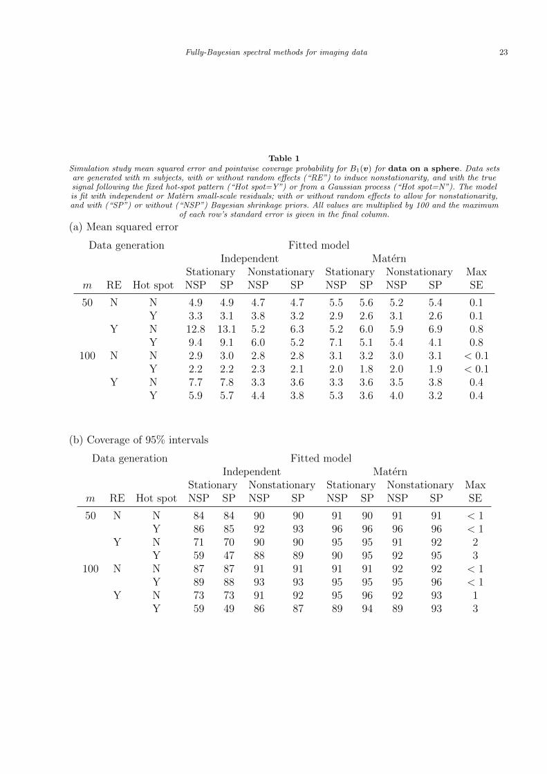
For each dataset we compute the posterior mean B1(v) and 95% equal-tailed credible set

[L1(v), U1(v)] for B1(v) for all voxels and then compute the spatial average mean squared

error∑

v[B1(v)− B1(v)]2/n and coverage∑

v I[L1(v) 6 B1(v) 6 U1(s)]/n. Table 1 reports

the average of the mean squared error and coverage across the 100 simulated datasets for

each scenario. The stationary model with independent residuals often has high MSE and low

coverage. For the models with independent residuals, adding the low-rank non-stationary

covariance improves performance, but coverage remains low in some cases. Coverage is at

or near the nominal 0.95 level for the full model for all scenarios. The inclusion of non-

stationarity and horseshoe priors improve performance in the anticipated settings.

[Table 1 about here.]

7. Analysis of the ADNI data

7.1 Model comparisons

In this section we apply the model proposed in Section 3 to the ADNI data. Unlike Section

3, the covariate effects do not have mean zero because for this application we do not expect

all fixed effects to be centered on zero (e.g., the confounder age should have an increasing

effect throughout the brain). Therefore we modify (5) to be E[Bk(v)] = Bk +∑J

j=1 Zj(v)βkj,

where the Bk is the overall mean and the βkj are have the same prior in as Section 3.

For our analysis we use L = 30 giving a reduction from 18,715 observations for each

subject in the spatial domain to 931 observations in the spectral domain. Exploratory

analysis in the Supplementary Materials (Figure 1) shows that terms beyond L = 30 do

Fully-Bayesian spectral methods for imaging data 11

not appear to contain additional spatial signal. As in Section 3, we allow for a different

set of spatial covariance parameters for the residual process Ei and the fixed effects Bk.

Preliminary analysis shows that the nugget variance is estimated to be near zero and so it

is excluded. Also, while we allow the six fixed effects terms to have a different variance σ2k,

we assume they have to same spatial range (φ) and smoothness parameter (ν) to improve

MCMC convergence. The overall effect Bk have normal priors with mean zero and variance

1,000, and for the remaining hyperparameters we use the same uninformative priors as in

Section 6. The MCMC algorithm is run for 100,000 iterations, the first 10,000 are discarded

as burn-in, and the remaining samples are thinned by 10 to remove autocorrelation. The full

model with Matern correlation, J = 225 basis functions, Horseshoe priors and nonstationary

covariance fit to these data takes around 11 minutes per 1,000 iterations.

We compare several methods using test set prediction. We randomly (across subject and

resolution) remove 10% of the Yi, fit the model to the remaining 90%, and evaluate the

agreement of the posterior predictive distributions and the test set observations. The models

fit vary by the specification of the residual correlation, fixed and random effects as in the simu-

lation study, and also the number of basis function J . Methods are compared in Table 2 using

mean squared error of the posterior predictive means, the average (across all observations)

of the posterior predictive variances, the empirical coverage of the 90% credible sets, and

the posterior predictive mean of the log-likelihood of the test set observations. Comparisons

are made by Legendre resolution in Supplementary Materials (Figure 2). Inclusion of the

Matern covariance is the most important factor in determining the predictive log-likelihood,

and including the nonstationary covariance with J = 225 also improves fit. For these data,

the Gaussian prior for fixed effects is sufficient, and we proceed with Gaussian priors for

the fixed effects and covariance that includes both the stationary Matern component and

non-stationary component with J = 225 basis functions.

12 Biometrics, 2017

[Table 2 about here.]

7.2 Results of the final model

Figure 2 summarizes the nonstationary component NS(v,v′) of the covariance in (4). The

standard deviation of the random effects ranges from 0.1-0.4; the standard deviation of the

response (across subject and location) is 0.53, so the nonstationary random effects account

for a substantial proportion of the variation. Figure 2 also maps the correlation in the

nonstationary component between three locations (indicated with black dots) and all other

locations, and show some interesting patterns. In Figure 2’s second row, all sites in the

superior/posterior region are strongly correlated. The bottom two rows reveal symmetries

between the left and right sides of the cortex in the posterior and anterior regions, respec-

tively, that clearly could not be captured by the stationary Matern correlation function.

[Figure 2 about here.]

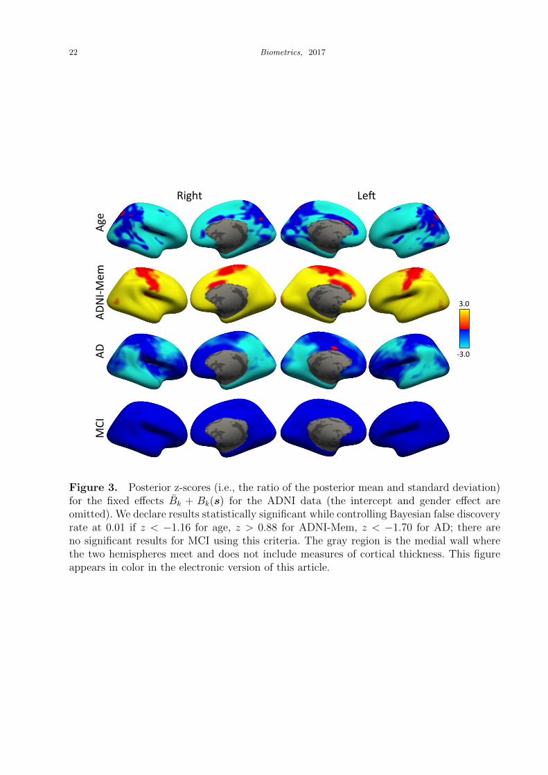
Posterior z-scores plotted in Figure 3. For the z-score maps, the threshold produced using

the method of Sun et al. (2015) to control Bayesian false discovery rate at 0.01 (separate for all

covariates) are given in the caption and statistically significant regions base on this threshold

are displayed in the Supplementary Materials (Figure 5). In this multiple testing problem, the

one-sided null and alternative hypotheses are H0 : βk(s) > 0 and H1 : βk(s) < 0, respectively,

for each covariate except ADNI-Mem which uses H0 : βk(s) 6 0 and H1 : βk(s) > 0.

These plots broadly resemble the least squares results in Figure 1, but are smoother and

in some cases reveal stronger results. Age and ADNI-Mem are the strongest predictors.

Age is negatively correlated with the response throughout the cortex and has the strongest

estimates in the anterior, specifically in the bilateral parahippocampal gyrus, temporal pole,

dorsolateral prefrontal cortex, and superior frontal cortex. ADNI-Mem is positively correlated

throughout the brain with the largest estimates in the anterior/inferior region, including

bilaterally in precuneus, middle and inferior temporal lobes, and medial orbitofrontal gyrus.

Fully-Bayesian spectral methods for imaging data 13

[Figure 3 about here.]

Much of the spatial variation in the voxel-at-a-time MCI regression coefficients (Figure 1,

bottom row) is smoothed out by the spatial model, and as a result none of the posterior

z-scores are significant in the spatial model. Also, the largest least squares effects for AD are

smoothed towards zero, suggesting these positive effects AD may be spurious associations.

However, AD is associated with significantly thinner cortex bilaterally in the inferior tem-

poral lobes (including the parahippocampal gyrus), the occipitoparietal junction and dorsal

prefrontal cortex. These regions overlap with well-established findings of parahippocampal

atrophy in the ADNI by Greene et al. (2010), and are understood to be involved in the

earlier stages of pathology (Braak and Braak, 1991). Atrophy in occipitoparietal junction is

another well-documented change, and pronounced pathology in this area has been associated

with a posterior cortical variant of AD (e.g., Crutch et al., 2012) which manifests in more

visuospatial and visuoperceptive deficiencies. Predominant atrophy of the frontal cortex

accompanies the frontal variant of AD which manifests in behavioral changes (Dubois et al.,

2014). Many of these regions overlap with those found to be associated with ADNI-Mem

scores (Nho et al., 2012).

8. Discussion

In this paper, we proposed a spectral spatial model for large imaging data sets. The model

accommodates features often seen in brain imaging data including nonstationary spatial

covariance and local covariate effects. The spherical harmonics transformation permit a fully-

Bayesian application to large datasets while respecting the spherical nature of the data. Using

simulated data we show that properly accounting for residual spatial correlation is necessary

for efficient estimation and valid inference. When applied to the ADNI data we find that

14 Biometrics, 2017

both stationary Matern and low-rank nonstationary covariance terms improve fit, and that

spatial methods identify regions of the cortex that differ by Alzheimer’s disease status.

We have focused on multi-subject studies, however our methods could be applied for a

single-subject study where data is collected over time. For example, after a discrete Fourier

transform over time at each voxel (Kang et al., 2012) the images for different frequencies

can be considered as independent (analogous to independence across subjects) and the

proposed method can be applied. Another area of future work is to improve computation

by exploiting parallel computing. The likelihood factors across subjects and frequencies, and

therefore likelihood evaluations are embarrassingly parallelizable and many parameters could

be updated in parallel which might improve computation time by an order of magnitude.

9. Supplementary Materials

Web Figures and R code referenced in Sections 2, 5 and 7 are available with this paper at

the Biometrics website on Wiley Online Library.

Acknowledgments

This research was partially supported NIH awards RO1NS085211 (AS and RTS), R21NS093349

(RTS), and T32MH065218 (SNV) and NSF award MS-1613219 (JG). Data collection and

sharing was funded by the Alzheimer’s Disease Neuroimaging Initiative (ADNI) (National

Institutes of Health Grant U01 AG024904) and DOD ADNI (DOD W81XWH-12-2-0012).

ADNI is funded by the National Institute on Aging, the National Institute of Biomedical

Imaging and Bioengineering, and through generous contributions. The Canadian Institutes

of Health Research is providing funds to support ADNI clinical sites in Canada. Private

sector contributions are facilitated by the Foundation for the National Institutes of Health

(www.fnih.org). The grantee organization is the Northern California Institute for Research

and Education, and the study is coordinated by the Alzheimers Therapeutic Research

Fully-Bayesian spectral methods for imaging data 15

Institute at the University of Southern California (USC). ADNI data are disseminated by

the Laboratory for Neuro Imaging at USC. The authors thank

http://adni.loni.usc.edu/wp-content/uploads/how_to_apply/

%ADNI_Acknowledgement_List.pdf

References

Bowman, F. D. (2007). Spatiotemporal models for region of interest analyses of functional

neuroimaging data. Journal of the American Statistical Association 102, 442–453.

Braak, H. and Braak, E. (1991). Neuropathological stageing of Alzheimer-related changes.

Acta Neuropathologica 82, 239–259.

Brookmeyer, R., Johnson, E., Ziegler-Graham, K., and Arrighi, H. M. (2007). Forecasting

the global burden of Alzheimers disease. Alzheimer’s & Dementia 3, 186–191.

Carvalho, C. M., Polson, N. G., and Scott, J. G. (2010). The horseshoe estimator for sparse

signals. Biometrika 97, 465–480.

Castruccio, S. and Guinness, J. (2017). An evolutionary spectrum approach to incorporate

large-scale geographical descriptors on global processes. Journal of the Royal Statistical

Society: Series C in press.

Castruccio, S., Ombao, H., and Genton, M. (2016). A multi-resolution spatio-temporal model

for brain activation and connectivity in fMRI data https://arxiv.org/abs/1602.02435.

Crane, P. K., Carle, A., Gibbons, L. E., et al. (2012). Development and assessment of a

composite score for memory in the Alzheimers Disease Neuroimaging Initiative (ADNI).

Brain Imaging and Behavior 6, 502–516.

Crutch, S. J., Lehmann, M., Schott, J. M., Rabinovici, G. D., Rossor, M. N., and Fox, N. C.

(2012). Posterior cortical atrophy. The Lancet Neurology 11, 170–178.

Dickerson, B. C., Feczko, E., Augustinack, J. C., Pacheco, J., Morris, J. C., Fischl, B., and

16 Biometrics, 2017

Buckner, R. L. (2009). Differential effects of aging and Alzheimer’s disease on medial

temporal lobe cortical thickness and surface area. Neurobiology of Aging 30, 432–440.

Dubois, B., Feldman, H. H., Jacova, C., et al. (2014). Advancing research diagnostic criteria

for Alzheimer’s disease: the IWG-2 criteria. The Lancet Neurology 13, 614–629.

Fischl, B. and Dale, A. M. (2000a). Measuring the thickness of the human cerebral cortex

from magnetic resonance images. Proceedings of the National Academy of Sciences 97,

11050–11055.

Fischl, B. and Dale, A. M. (2000b). Measuring the thickness of the human cerebral cortex

from magnetic resonance images. Proceedings of the National Academy of Sciences 26,

11050–11055.

Fuentes, M. and Reich, B. J. (2010). Spectral domian. In Gelfand, A. E., Diggle, P. J.,

Fuentes, M., and Guttorp, P., editors, Handbook of Spatial Statistics, chapter 5. Chapman

& Hall/CRC Press.

Greene, S. J., Killiany, R. J., and Alzheimer’s Disease Neuroimaging Initiative (ADNI)

(2010). Subregions of the inferior parietal lobule are affected in the progression to

Alzheimer’s disease. Neurobiology of Aging 31, 1304–1311.

Guinness, J. and Fuentes, M. (2016). Isotropic covariance functions on spheres: Some

properties and modeling considerations. Journal of Multivariate Analysis 143, 143–152.

Handcock, M. S. and Stein, M. L. (1993). A Bayesian analysis of Kriging. Technometrics

35, 403–410.

Hyun, J. W., Li, Y. M., Gilmore, J., et al. (2014). SGPP: Spatial Gaussian predictive process

models for neuroimaging data. NeuroImage 89, 70–80.

Jack, C. R., Bernstein, M. A., Fox, N. C., et al. (2008). The Alzheimer’s disease neuroimaging

initiative (ADNI): MRI methods. Journal of Magnetic Resonance Imaging 27, 685–691.

Kang, H., Ombao, H., Linkletter, C., Long, N., and Badre, D. (2012). Spatio-spectral mixed-

Fully-Bayesian spectral methods for imaging data 17

effects model for functional magnetic resonance imaging data. Journal of the American

Statistical Association 107, 568–577.

Lange, N. and Zeger, S. L. (1997). Non-linear fourier time series analysis for human brain

mapping by functional magnetic resonance imaging. Journal of the Royal Statistical

Society: Series C (Applied Statistics) 46, 1–29.

Lerch, J. P., Pruessner, J., Zijdenbos, A. P., Collins, D. L., Teipel, S. J., Hampel, H.,

and Evans, A. C. (2008). Automated cortical thickness measurements from MRI can

accurately separate Alzheimer’s patients from normal elderly controls. Neurobiology of

Aging 29, 23–30.

Lerch, J. P., Pruessner, J. C., Zijdenbos, A., Hampel, H., Teipel, S. J., and Evans, A. C.

(2005). Focal decline of cortical thickness in Alzheimer’s disease identified by computa-

tional neuroanatomy. Cerebral Cortex 15, 995–1001.

McKhann, G., Drachman, D., Folstein, M., Katzman, R., Price, D., and Stadlan, E. M.

(1984). Clinical diagnosis of Alzheimer’s disease Report of the NINCDS-ADRDA Work

Group* under the auspices of Department of Health and Human Services Task Force on

Alzheimer’s Disease. Neurology 34, 939–939.

Mueller, S. G., Weiner, M. W., Thal, L. J., et al. (2005). Ways toward an early diagnosis in

Alzheimers disease: the Alzheimers Disease Neuroimaging Initiative (ADNI). Alzheimer’s

& Dementia 1, 55–66.

Musgrove, D. R., Hughes, H., and Eberly, L. E. (2017). Fast, fully Bayesian spatiotemporal

inference for fMRI data. Biostatistics In press.

Nho, K., Risacher, S. L., Crane, P. K., et al. (2012). Voxel and surface-based topography

of memory and executive deficits in mild cognitive impairment and Alzheimer’s disease.

Brain Imaging and Behavior 6, 551–567.

Rocca, W. A., Petersen, R. C., Knopman, D. S., Hebert, L. E., et al. (2011). Trends in the

18 Biometrics, 2017

incidence and prevalence of Alzheimers disease, dementia, and cognitive impairment in

the United States. Alzheimer’s & Dementia 7, 80–93.

Sled, J. G., Zijdenbos, A. P., and Evans, A. C. (1998). A nonparametric method for

automatic correction of intensity nonuniformity in MRI data. IEEE Transactions on

Medical Imaging 17, 87–97.

Spence, J., Carmack, P., Gunst, R., Schucany, W., Woodward, W., and Haley, R. (1997).

Accounting for spatial dependence in the analysis of SPECT brain imaging data. Journal

of the American Statistical Association 102, 464–473.

Stein, M. (1999). Statistical interpolation of spatial data: Some theory for Kriging. Springer,

New York.

Stein, M. L. (2014). Limitations on low rank approximations for covariance matrices of

spatial data. Spatial Statistics 8, 1–19.

Sun, W., Reich, B. J., Cai, T., Guindani, M., and Schwartzman, A. (2015). False discovery

control in large-scale spatial multiple testing. Journal of the Royal Statistical Society:

Series B 77, 59–77.

Wimo, A., Jonsson, L., and Winblad, B. (2006). An estimate of the worldwide prevalence

and direct costs of dementia in 2003. Dementia and Geriatric Cognitive Disorders 21,

175–181.

Woolrich, M., Jenkinson, M., Brady, J., and Smith, S. (2004). Fully Bayesian spatio-temporal

modeling of fMRI data. IEEE Transactions on Medical Imaging 23, 213–231.

Yaglom, A. M. (2012). Correlation theory of stationary and related random functions.

Springer Science & Business Media.

Zhang, L., Guindani, M., Versace, F., et al. (2016). A spatiotemporal nonparametric Bayesian

model of multi-subject fMRI data. The Annals of Applied Statistics 10, 638–666.

Zhang, L., Guindani, M., Versace, F., and Vannucci, M. (2014). A spatio-temporal non-

Fully-Bayesian spectral methods for imaging data 19

parametric Bayesian variable selection model of fMRI data for clustering correlated time

courses. NeuroImage 95, 162–175.

Zhu, H., Fan, J., and Kong, L. (2014). Spatially varying coefficient model for neuroimaging

data with jump discontinuities. Journal of the American Statistical Association 109,

1084–1098.

Received: April 19, 2017

20 Biometrics, 2017

Right Le)

AD

Age

3.0

-3.0

ADNI-M

em

MCI

Figure 1. Z-scores for the covariate effects from ordinary least squares conducted sepa-rately for each location (the intercept and gender effect are omitted). The gray region isthe medial wall where the two hemispheres meet and does not include measures of corticalthickness. This figure appears in color in the electronic version of this article.

Fully-Bayesian spectral methods for imaging data 21

Right Le)

Cor2

SD

Co

r1

Cor3

1.0

0.0

0.19

0.0

Figure 2. Summaries of the posterior mean of the nonstationary covariance NS(v,v′)in (3). The top row gives the standard deviation

√NS(v,v) and the remaining rows plot

the correlation NS(v,v′)/√NS(v,v)NS(v′,v′) across v for three points v′ denoted with

black dots. The gray region is the medial wall where the two hemispheres meet and does notinclude measures of cortical thickness. This figure appears in color in the electronic versionof this article.

22 Biometrics, 2017

Right Le)

AD

Age

3.0

-3.0

ADNI-M

em

MCI

Figure 3. Posterior z-scores (i.e., the ratio of the posterior mean and standard deviation)for the fixed effects Bk + Bk(s) for the ADNI data (the intercept and gender effect areomitted). We declare results statistically significant while controlling Bayesian false discoveryrate at 0.01 if z < −1.16 for age, z > 0.88 for ADNI-Mem, z < −1.70 for AD; there areno significant results for MCI using this criteria. The gray region is the medial wall wherethe two hemispheres meet and does not include measures of cortical thickness. This figureappears in color in the electronic version of this article.

Fully-Bayesian spectral methods for imaging data 23

Table 1Simulation study mean squared error and pointwise coverage probability for B1(v) for data on a sphere. Data setsare generated with m subjects, with or without random effects (“RE”) to induce nonstationarity, and with the truesignal following the fixed hot-spot pattern (“Hot spot=Y”) or from a Gaussian process (“Hot spot=N”). The modelis fit with independent or Matern small-scale residuals; with or without random effects to allow for nonstationarity,and with (“SP”) or without (“NSP”) Bayesian shrinkage priors. All values are multiplied by 100 and the maximum

of each row’s standard error is given in the final column.

(a) Mean squared error

Data generation Fitted modelIndependent Matern

Stationary Nonstationary Stationary Nonstationary Maxm RE Hot spot NSP SP NSP SP NSP SP NSP SP SE

50 N N 4.9 4.9 4.7 4.7 5.5 5.6 5.2 5.4 0.1Y 3.3 3.1 3.8 3.2 2.9 2.6 3.1 2.6 0.1

Y N 12.8 13.1 5.2 6.3 5.2 6.0 5.9 6.9 0.8Y 9.4 9.1 6.0 5.2 7.1 5.1 5.4 4.1 0.8

100 N N 2.9 3.0 2.8 2.8 3.1 3.2 3.0 3.1 < 0.1Y 2.2 2.2 2.3 2.1 2.0 1.8 2.0 1.9 < 0.1

Y N 7.7 7.8 3.3 3.6 3.3 3.6 3.5 3.8 0.4Y 5.9 5.7 4.4 3.8 5.3 3.6 4.0 3.2 0.4

(b) Coverage of 95% intervals

Data generation Fitted modelIndependent Matern

Stationary Nonstationary Stationary Nonstationary Maxm RE Hot spot NSP SP NSP SP NSP SP NSP SP SE

50 N N 84 84 90 90 91 90 91 91 < 1Y 86 85 92 93 96 96 96 96 < 1

Y N 71 70 90 90 95 95 91 92 2Y 59 47 88 89 90 95 92 95 3

100 N N 87 87 91 91 91 91 92 92 < 1Y 89 88 93 93 95 95 95 96 < 1

Y N 73 73 91 92 95 96 92 93 1Y 59 49 86 87 89 94 89 93 3

24 Biometrics, 2017

Table 2Cross validation results for the ADNI data. The methods fit to the data vary by the residual correlation of E; the

prior for the fixed effects (“FE”) B, the inclusion of the nonstationary subject random effects (“nonstationary”) Z,and the number of basis functions J . Methods are compared by the average (over all test set observations) of logprediction likelihood (“Log Like”), mean squared prediction error (“MSE”), average prediction variance (“Var”);

and coverage of 90% prediction intervals (“Cov”).

Residuals FE Nonstationary J Log Like MSE Var Cov90

Independent Gaussian No 25 -0.945 0.372 0.591 0.959Independent Gaussian No 225 -0.945 0.372 0.591 0.959Independent Gaussian Yes 25 -0.907 0.435 0.334 0.919Independent Gaussian Yes 225 -1.087 0.327 0.295 0.895Independent Horseshoe No 25 -0.945 0.372 0.591 0.959Independent Horseshoe No 225 -0.945 0.372 0.590 0.960Independent Horseshoe Yes 25 -0.907 0.435 0.334 0.919Independent Horseshoe Yes 225 -1.088 0.329 0.295 0.895

Matern Gaussian No 25 -0.520 0.371 0.530 0.901Matern Gaussian No 225 -0.520 0.371 0.530 0.901Matern Gaussian Yes 25 -0.513 0.385 0.342 0.901Matern Gaussian Yes 225 -0.529 0.313 0.302 0.900Matern Horseshoe No 25 -0.520 0.372 0.530 0.901Matern Horseshoe No 225 -0.520 0.372 0.530 0.902Matern Horseshoe Yes 25 -0.512 0.385 0.342 0.901Matern Horseshoe Yes 225 -0.529 0.313 0.301 0.900