Appl Phys A (2012) 107:575–582DOI 10.1007/s00339-012-6832-7

I N V I T E D PA P E R

Spectral density representation of dielectric mixtures

Enis Tuncer

Received: 26 September 2011 / Accepted: 10 February 2012 / Published online: 29 February 2012© Springer-Verlag 2012

Abstract Dielectric relaxation has attracted lot of interestsince the days of J.C. Maxwell. Although relaxation in pure,single materials is a puzzling topic, relaxation in mixtureshas its own perplexing sides. However, with the help of spec-tral density representation, one has the possibility to separatecontributions of the constituents and the geometrical compo-sition of the mixture phases. Here, we will present the theoryof dielectric mixtures with the spectral density representa-tion. It will be shown that depending on the dielectric prop-erties and geometrical description of the constituents differ-ent effective permittivity can be obtained for a chosen pair ofmixture components—binary mixtures. The tools presentedhere can be used to better understand the dielectric proper-ties of materials. The numerical implementations presentedfor immittance data can be used for various physical prop-erties of heterogeneous materials. For mixtures, they pro-vide great value in (i) designing the permittivity of a mix-ture composed of substances with known permittivities andgeometrical composition (for device and insulation applica-tions), (ii) calculating the permittivity of the second com-ponent of a two-component mixture when the permittivitiesof the mixture and the first component are known (for ma-terial and system characterization), and (iii) estimating themorphology of a two-component mixture when the permit-

The manuscript is dedicated to Professor Reimund Gerhard for hiskindness, fruitful discussion and guidance in my research andprofessional life.

E. Tuncer (�)Dielectrics & Electrophysics Lab, GE Global Research Center,Niskayuna, NY 12309, USAe-mail: tuncer@ge.com

E. Tuncere-mail: enis.tuncer@physics.org

tivities of the mixture and each of the components are known(for microstructure and structure/property relationships).

1 Introduction

Many materials used in daily applications are composites,which are often made up of at least two components. Elec-trical and dielectric properties of these heterogeneous ma-terials have been a topic of interest for many decades withpioneering works [1–10], where the simplest case with two-component (binary) mixtures has been the focus. The inter-est never abated and several books [11–16] and review pa-pers [17–28] were published on the topic. The majority ofwork was performed on static properties.

Simulations and analytical modeling performed withcomplex permittivities have investigated only properties atconstant frequencies [24, 29–34], while very few articlesconcentrated on the frequency dispersion of binary mix-tures [25, 35–38]. The beauty of investigating the frequencydependent properties of binary mixtures has been manyfolded; (i) information on system structural properties andhow particle shape and dispersion influence the overall com-posite properties can be studied; (ii) fundamentals of dielec-tric relaxation and interacting systems can be investigated;(iii) the nature of real systems such as polymers, ionic liq-uids, etc. can be elucidated with detailed analysis, for ex-ample, by taking into account the structure of monomersand branched structure; (iv) the generated understandingof system dynamics and structure/property relationship canbe employed to design functional materials, devices, and aswell as diagnostics tools for assessing health of various sys-tems with electrical measurements. Notice that one of theneglected areas in dielectric sciences is the correlation be-tween the synthetic dispersion data of binary mixtures and

576 E. Tuncer

those observed in real polymeric composites and even poly-mers, which contain a complex blend of polarizable unitsand dipoles—also a mixture of phases, a sophisticated one.Polymers are molecular systems composed of various dipo-lar units. Depending on the length scale of interest, they maybe considered dielectric mixtures, either mixtures of dipolesin nanoscale or mixtures of dipolar regions with differentelectrical properties in microscale. The spectral representa-tion can be employed to improve our understanding of thedielectric dispersion in these systems.

The main message of this paper will be the applicationof the spectral density representation. The synthetic datawere generated with constituents having complex permit-tivities. It will be shown that the dispersion of the effec-tive permittivity of a composite can be significantly dif-ferent than the both components due to the introduced in-tricate dielectric dispersion with charge polarization at theconstituent interfaces—interfacial polarization. The polar-ized charge yields different depolarization factors depend-ing on the topology of the interface. Influence of differentdepolarization factors or spectral parameters, in other wordsthe inclusion phase shape, and concentration will be demon-strated.

2 Background

2.1 Electrical properties of materials

The immittance data of a material can be represented in dif-ferent levels [39–42] (i) the complex resistivity ρ∗(ω), (ii)the complex modulus M∗(ω) ≡ ıωε0ρ

∗(ω), (iii) the relativecomplex permittivity ε∗(ω) ≡ [M∗(ω)]1, and (iv) the com-plex conductivity σ ∗(ω) ≡ ıωε0ε

∗(ω) ≡ [ρ∗(ω)]1, whereı ≡ √−1, ω is the angular frequency and ε0 is the permit-tivity of vacuum and equal to 8.854 pF m−1.

Throughout the current presentation, complex permittiv-ity level is used, however, the employment of the complexresistivity can be appropriate in some cases as shown later inthe text. The frequency dependent complex permittivity of amaterial is presented as

ε∗(ω) = ε∞ + σ0(ıε0ω)−1 + χ∗(ω), (1)

= ε′ − ıε′′. (2)

Here, ε∞ and σ0 are frequency independent material con-stants and can be estimated from data using differentmethods—nonlinear complex curve fitting using a modelexpression for the whole ε∗(ω), nonparametric curve fittingusing distribution of relaxation times or the Kramer–Kronigrelationship, which would allow ε∞ to be estimated fromthe high frequency region of the imaginary part of com-plex permittivity ε∗(ω) and σ0 estimated from the low fre-quency region of the real part of the complex permittivity

ε∗(ω). The real and imaginary parts of the permittivity areexpressed with ε′ and ε′′, respectively. One could anticipateto obtain σ0 from the complex resistivity ρ∗(ω), however,the contribution of ohmic losses is usually not clearly visi-ble due to either lack of data at low enough frequencies inthe measurements or the presence of electrode polarization,which is present in many materials with nonelectronic con-duction [43–46]. In theory at low enough frequencies—afterall the polarization processes are finalized, totally polarizedmaterial—the imaginary part of the complex resistivity ρ∗should converge to zero,

�[ρ∗(ω → 0)

] = 0

while the real part of the complex resistivity ρ∗ should con-verge to inverse ohmic conductivity of the material,

[ρ∗(ω → 0)

] = σ−10 .

Similarly in theory at high enough frequencies, instanta-neous polarization due to fast moving charging would con-tribute to the polarization as a constant, which is definedas the high frequency permittivity ε∞, much higher fre-quencies than the highest frequency in the measurement fre-quency range,

[ε∗(ω → ∞)

] = ε∞.

All the frequency dependent polarization and conductionprocesses would be included in the complex susceptibil-ity χ∗(ω) in (1). Different analytical and empirical expres-sions have been reported to describe the immittance data.Some concrete examples are Debye [47], Dissado–Hill [48],Havriliak–Negami [49, 50], Cole-Cole [51], Davidson-Cole [52], stretched exponential [41, 53], etc. Nonparamet-ric dielectric data analysis methods based on the distributionof relaxation times [54–56] were proposed to better under-stand relaxation phenomenon in dielectrics.

2.2 Spectral density representation

Knowing the spectral density function one can estimatethe shape(s) and their distribution in a composite mate-rial. The representation proposed earlier [26, 57–59] andthe simplified version [42, 60] separates intrinsic propertiesof constituents in a composite material from how the con-stituents are arranged. Actually the spectral density is re-lated to the depolarization factors of constituents in dielec-tric mixtures [61–68]. Simple Euclidean shapes, disk, el-lipse, sphere, cylinders, spheroid, etc., would result in delta-function spectral functions, however, any polydispersity andshape deviations would broaden the spectra. The simplifiedeffective medium function based on the spectral density rep-resentation is as follows:

ξ =∫ 1

0g(x)(1 + x)−1 dx, (3)

Spectral density representation of dielectric mixtures 577

where ξ is the complex scaled permittivity,

ξ = (ε − ε1)(ε2 − ε1)−1, (4)

here all the parameters are complex variables, ε is the ef-fective permittivity, and ε1 and ε2 are constituent permit-tivities. The parameters and x are the probing spectralfrequency and spectral parameter, respectively, in (3). Theprobing spectral frequency is expressed with the constituentpermittivities,

= ε2(ε1)−1 − 1. (5)

The spectral frequency cannot directly be measured exper-imentally, however, it is completely depending on the con-stituent permittivities, which are measurable quantities. Thedistribution of shapes or the spectral density function is g(x)

in (3). The limits of the integration in (3) is defined from 0to 1. However, for fractals with dimensionality less than 1,the upper limit needs to be modified—upper limit can belarger than 1.

One needs to modify (3) to define two different structuralcharacteristics in composites, finite and infinite clusters or inother words nonpercolating and percolating paths. The non-percolating structures contribute to the dielectric dispersionas Maxwell–Wagner–Sillars (interfacial) polarization due toclear interface between the constituents. However, the per-colating structures does not generate such contributions. Theextremes of these conditions are the Wiener bounds in di-electric mixtures [69], where fully nonpercolating and lay-ered and percolating layered geometries are considered—the spectral parameters 1 and 0 correspond to nonpercolat-ing and percolating parameters, respectively. With the con-sideration of structural differences between percolating andnonpercolating parts of in a composite, we separate the per-colating clusters as follows using (3):

g(x) = δ(x) (6)

ξ = g(0). (7)

Here, we represent the pole at zero, g(0), with ξp—percolating part contributions in the scaled permittivity,xp ≡ g(0).

The variable ξp is the fraction of phase 2 in phase 1 thatis percolating. The altered scaled permittivity then becomes

ξ = ξp +∫ k

0+g(x)(1 + x)−1 dx. (8)

Observe that the integral upper limit is generalized to k. De-pending on the shapes of inclusions existing in the mixture k

would be different. Even k larger than 1 can be imagined iffractal-like shapes are involved in a mixture. The propertiesof g(x) determine structural information in a binary com-posite. It will be shown later that x > 1 case is possible for

dielectric mixtures, since obtained effective permittivity hasa physical dispersion that does not violate the complex per-mittivity relationship. Integration of spectral function g(x) isthe fraction of phase 2 that is nonpercolating, defined withξn. The most expected value of spectral parameter x yieldsthe most expected shape in a binary composite which hasbeen discussed in the literature [70, 71]. Below are the prop-erties of spectral function g(x),

∫ k

0+g(x)dx = ξn (9)

∫ k

0+xg(x)dx = (1 − ξn)d

−1. (10)

Here, d is the dimensionality, however, it can also be relatedto the depolarization factor in simple shapes, i.e., for spheresd = 3. It should be noted that the right-hand side of (10)couples the physical parameter concentration to dimension-ality. It would be hard to decouple these two parametersin complex geometries. It has been shown previously thatthe expected value for x can be estimated accurately withinverse problem approaches for dilute mixtures [71] andMaxwell Garnett expression [72]. There could be severalpeaks, meaning that there are several structural features, inthat case the integrals would be estimated with other lowerand upper limits as follows:

∫ b

a

g(x)dx = ξn (11)

∫ b

a

xg(x)dx = (1 − ξn)d−1. (12)

While deviations from the expected values are observedwhen concentration of the inclusions are high indicating thatthe dimensionality either changed or the depolarization fac-tor diverge from the expected value due to interaction be-tween inclusion particles. The total concentration Q of phase2 can be expressed as

ξp + ξn = Q. (13)

In the present illustrations, we consider a delta functionfor the spectral function,

g(x) = ξnδ[x − (1 − ξn)d

−1], (14)

a simple dielectric mixture expression can be generated us-ing the integral in (8),

ξ = ξp + ξnd[d + (1 − ξn)

]−1. (15)

Several different mixture dielectric dispersions are gener-ated with (15). The dimensionality is altered between 0.1and 1000. Although d < 1 is the first time introduced in di-electric mixtures, structures with d < 1 exist in fractals—in

578 E. Tuncer

Table 1 Material parameters used in the simulations

Phase ε∞ σ0 [S/m] η [S/m] γ Δ τ [s] α

1 2 10−12 10−14 0.5 0.1 0.1 0.8

2 10 10−10 10−12 0.7 0.1 0.01 0.1

the Nature. Knowing the fractal dimension could be infor-mative, however, just like the orientation of spheroidal, par-allel, or perpendicular to field direction, the fractal dimen-sion would be of importance to determine the depolariza-tion factor. For example, Cantor set geometry in or out offield plane views would have different fractal dimensions.For the Cantor set out of field plane, a fractal dimension d

of less than 1 could be expected yielding a depolarizationfactor higher than 1.

3 Model binary dielectric

The constituents were assumed to have complex permittiv-ity not only with ohmic losses as conventional approach,where (1) is expressed without the complex susceptibil-ity but with complex susceptibility and low frequency dis-persion. Most of the materials in nature have (or exhibit)complex susceptibilities when the dielectric response is ex-pressed on a broad frequency range. The permittivities ofphase 1 and 2 are as follows in the current simulations:

ε∗1(ω) = ε∞1 + σ01(ıε0ω)−1 + χ∗

1 (ω) with (16)

χ∗1 (ω) = η1(ıω)γ1 + Δ1

[1 + (ıτ1ω)α1

]−1 (17)

ε∗2(ω) = ε∞2 + σ02(ıε0ω)−1 + χ∗

2 (ω) with (18)

χ∗2 (ω) = η2(ıω)γ2 + Δ2(1 + ıτ2ω)−α2 . (19)

Here, we have both a dielectric relaxation with broad dis-tribution function described with Cole–Cole and Cole–Davidson functions. We have also included a low frequencydispersion for both phases to further implement a completedispersion to the constituent permittivities. The material pa-rameters employed in the simulations are presented in Ta-ble 1.

4 Simulation results and discussion

The permittivity of the constituents and the composites withdifferent d are shown in Fig. 1. The concentration of the con-stituent are kept constant for nonpercolating part ξn = 0.5and no percolation contribution is included ξp = 0. It isclear in the imaginary part of the permittivity ε′′ that the val-ues are between the two constituent complex permittivities,

Fig. 1 Complex permittivity of a mixture composed of two con-stituents with complex dielectric permittivities. The dark lines indicatethe dielectric properties of the constituents. It is straightforward to dif-ferentiate the responses at high frequencies (above 10 cps) in the realpart of the permittivity ε′(ω) with regard to the mixture and constituentresponses. However, at low frequencies (between 1 mcps and 10 cps),there are cases that the permittivity of the mixture is higher than thepermittivity of the constituents. This is due to the interfacial polariza-tion. The arrows indicate the increasing dimensionality values that areconsidered in the simulations

lower limit is ε′′1 and upper limit is ε′′

2 . The permittivities ofcomposites indicate different dispersions with changing d

value—higher the d-value higher the real part of the permit-tivity at low frequencies. One can achieve a higher permittiv-ity than both phases for d > 5 between 1 ms−1 and 1 s−1 asshown in Fig. 1. For the considered cases, the complex sus-ceptibilities are shown in Fig. 2, which illustrates the dielec-tric dispersions more clearly than the permittivity level. It isnot always easy to obtain the susceptibility level in real sys-tems due to exact calculation of high frequency permittivityε∞ and ohmic losses σ0 due to lack of broadband dielec-tric data and required Kramer–Kronig relations [55, 73, 74]

Spectral density representation of dielectric mixtures 579

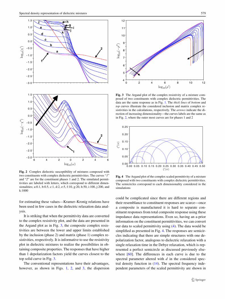
Fig. 2 Complex dielectric susceptibility of mixtures composed withtwo constituents with complex dielectric permittivities. The curves “1”and “2” are for the constituent phases 1 and 2. The simulated permit-tivities are labeled with letters, which correspond to different dimen-sionalities; a:0.1, b:0.5, c:1, d:2, e:5, f:10, g:20, h:50, i:100, j:200, andk:1000

for estimating these values—Kramer–Kronig relations havebeen used in few cases in the dielectric relaxation data anal-ysis.

It is striking that when the permittivity data are convertedto the complex resistivity plot, and the data are presented inthe Argand plot as in Fig. 3, the composite complex resis-tivities are between the lower and upper limits establishedby the inclusion (phase 2) and matrix (phase 1) complex re-sistivities, respectively. It is informative to use the resistivityplot in dielectric mixtures to realize the possibilities in ob-taining composite properties. The responses that have higherthan 1 depolarization factors yield the curves closest to thetop solid curve in Fig. 3.

The conventional representations have their advantages,however, as shown in Figs. 1, 2, and 3, the dispersion

Fig. 3 The Argand plot of the complex resistivity of a mixture com-posed of two constituents with complex dielectric permittivities. Thedata are the same response as in Fig. 1. The thick lines of bottom andtop curves illustrate the considered inclusion and matrix complex re-sistivities in the calculations, respectively. The arrows indicate the di-rection of increasing dimensionality—the curves labels are the same asin Fig. 2, where the outer most curves are for phases 1 and 2

Fig. 4 The Argand plot of the complex scaled permittivity of a mixturecomposed with two constituents with complex dielectric permittivities.The semicircles correspond to each dimensionality considered in thesimulations

could be complicated since there are different regions andtheir resemblance to constituent responses are scarce—oncea composite is manufactured it is hard to separate con-stituent responses from total composite response using theseimpedance data representations. Even so, having an a-priorinformation on the constituent permittivities, we can convertour data to scaled permittivity using (4). The data would besimplified as presented in Fig. 4. The responses are semicir-cles indicating that there are simple structures with one de-polarization factor, analogous to dielectric relaxation with asingle relaxation time in the Debye relaxation, which is rep-resented a perfect semicircle as discussed previously else-where [60]. The differences in each curve is due to thespectral parameter altered with d in the considered spec-tral density function in (14). The spectral frequency inde-pendent parameters of the scaled permittivity are shown in

580 E. Tuncer

Fig. 5 The low and high spectral frequency values of scaled permittiv-ity ξ∗, expressed with min and max values as a function of considereddifferent dimensionality

Fig. 6 The complex spectral frequency as a function of angularfrequency ω

Fig. 5. As observed in the Debye relaxation, the maximumof the imaginary part of the scaled permittivity �[ξ ] is halfof the real part of the scaled permittivity strength [Δξ ].The change in the scaled permittivity as a function of thedimensionality or the depolarization factor indicates that thehighest polarization would be observed at d = 1. Layered ar-rangement of phases perpendicular to the applied field gen-erates the highest effective permittivity via interfacial polar-ization [1, 3, 4, 8].

Observe that the spectral frequency is a complexnumber and its real and imaginary parts have a frequencydispersion as shown in Fig. 6. Although with the currentphase parameters the dispersion in resembles the Debyeresponse—a step in the real part and a loss peak in the imag-

Fig. 7 The complex scaled permittivity ξ∗ as a function of angularfrequency ω for different delta function spectral distributions g(x).The simulated scaled permittivities are labeled with letters, which cor-respond to different dimensionalities; a:0.1, b:0.5, c:1, d:2, e:5, f:10,g:20, h:50, i:100, j:200, and k:1000

Fig. 8 The effective ohmic conductivity normalized with vacuum per-mittivity σe

0 (ε0) as a function of effective high frequency permittivityεe∞ for different dimensionality d−1, shown next to each data point.Different dimensionalities considered in the simulations were previ-ously used for labeling as a:0.1, b:0.5, c:1, d:2, e:5, f:10, g:20, h:50,i:100, j:200, and k:1000

inary part—it can have a more complicated dependence onthe frequency. The final dispersion we obtain is the complexscaled permittivity ξ∗ as a function of angular frequency asshown in Fig. 7 again for different selected spectral param-eters x via changing d in (10). The dependence of complexpermittivity on different spectral functions is clear. Whilethe values of expected x are changed on a large scale, therelaxation in scale permittivity is in a short range, between1 ms−1 to 100 s−1. Compared to the dispersion in com-

Spectral density representation of dielectric mixtures 581

plex permittivity and resistivity level, the dispersion of thecomplex scaled permittivity is less complicated for simplecomposites—current systems have only one spectral param-eter; g(τ ) is a delta function rather than a distribution.

The frequency independent parameters of the mixture ef-fective high frequency permittivity εe∞ and effective ohmicconductivity σ e

0 as a function of altered spectral parame-ter are shown in Fig. 8. As known from depolarization fac-tors of different shapes and their effect on effective prop-erties [8, 66], the higher the expected spectral parameterfrom (10) is higher the dielectric response and ohmic losseswill be. The consequences of this relationship is that notonly the intrinsic properties of the constituents are impor-tant, but one can also use the shape of the inclusions to tailorcomposites specific applications.

5 Conclusion

An attempt to present effective dielectric properties of abinary composite is demonstrated with constituents havingcomplex dielectric permittivities. Spectral density represen-tation is introduced to analyze the dielectric data of compos-ites which could have advantages over conventional meth-ods. It is shown that complex resistivity plot is a graphictool to display and analyze data.

References

1. J.C. Maxwell, A Treatise on Electricity and Magnetism, Vol. 1,3rd edn. (Clarendon Press, Oxford, 1891), pp. 450–464, reprint byDover

2. J.C.M. Garnett, Philos. Trans. R. Soc. Lond. A 203, 385 (1904)3. K.W. Wagner, Ann. Phys. 40, 817 (1913)4. K.W. Wagner, Archiv Electrotech II, 371 (1914)5. H. Fricke, Phys. Rev. 24, 575 (1924)6. H.H. Lowry, J. Franklin Inst. 203, 413 (1927)7. D.A.G. Bruggeman, Ann. Phys. (Leipz.) 24, 636 (1935)8. R. Sillars, J. Inst. Elect. Eng. 80, 378 (1937)9. R. Landauer, J. Appl. Phys. 23, 779 (1952)

10. H. Fricke, J. Phys. Chem. 57, 934 (1953)11. M. Sahimi, Heterogeneous Materials I: Linear Transport and Op-

tical Properties, vol. 22 (Springer, Berlin, 2003)12. S. Torquato, Random Heterogeneous Materials: Microstructure

and Macroscopic Properties, vol. 16 (Springer, Berlin, 2001)13. R. Landauer, in Electrical Transport and Optical Properties of In-

homogeneous Media, ed. by J.C. Garland, D.B. Tanner. AIP Con-ference Proceedings, vol. 40 (American Institute of Physics, NewYork, 1978), pp. 2–43

14. A. Sihvola, Electromagnetic Mixing Formulas and Applications,IEE Electromagnetic Waves Series, vol. 47 (The Institute of Elec-trical Engineers, London, 1999)

15. G.W. Milton, The Theory of Composites, Cambridge Monographson Applied and Computational Mathematics, vol. 6 (CambridgeUniversity Press, Cambridge, 2002)

16. A. Priou (ed.), Progress in Electromagnetics Research, Dielec-tric Properties of Heterogeneous Materials (Elsevier, New York,1992)

17. P.A.M. Steeman, J. van Turnhout, in Broadband Dielectric Spec-troscopy, ed. by F. Kremer, A. Schönhals (Springer, Berlin, 2003),pp. 495–522

18. W.R. Tinga, in Dielectric Properties of Heterogeneous Materials.Progress in Electromagnetic Research, vol. 6 (Elsevier, Amster-dam, 1992), pp. 1–40, Chap. 1

19. Y.P. Emets, Y.V. Obnosov, Sov. Phys. Tech. Phys. 35, 907 (1990)20. Y.P. Emets, Y.V. Obnosov, Sov. Phys. Dokl. 34, 972 (1989)21. K. Golden, G. Papanicolaou, Commun. Math. Phys. 90, 473

(1983)22. H. Looyenga, Physica 31, 401 (1965)23. A. Sihvola, Subsurf. Sensing Technol. Appl. 1, 393 (2000)24. C. Brosseau, A. Beroual, Progress. Mater. Sci. 48, 373 (2003)25. E. Tuncer, Y.V. Serdyuk, S.M. Gubanski, IEEE Trans. Dielectr.

Electr. Insul. 9, 809 (2002)26. D.J. Bergman, Phys. Rep. 43, 377 (1978)27. G.A. Niklasson, C.G. Granqvist, J. Appl. Phys. 55, 3382 (1984)28. G.A. Niklasson, J. Appl. Phys. 57, 157 (1985)29. C. Brosseau, A. Beroual, J. Phys. D, Appl. Phys. 34, 704 (2001)30. A. Boudida, A. Beroual, C. Brosseau, J. Appl. Phys. 88, 7278

(2000)31. C. Brosseau, A. Beroual, Eur. Phys. J. Appl. Phys. 6, 23 (1999)32. B. Sareni, L. Krähenbühl, A. Beroual, A. Nicolas, C. Brosseau, J.

Electrost. 40 & 41, 489 (1997)33. B. Sareni, L. Krähenbühl, A. Beroual, C. Brosseau, J. Appl. Phys.

81, 2375 (1997)34. D. Gershon, J.P. Calame, A. Birnboim, J. Appl. Phys. 89, 8110

(2001)35. E. Tuncer, B. Nettelblad, S.M. Gubanski, J. Appl. Phys. 92, 4612

(2002)36. E. Tuncer, S.M. Gubanski, B. Nettelblad, J. Appl. Phys. 89, 8092

(2001)37. E. Tuncer, Ph.D. thesis, Chalmers University of Technology,

Gothenburg, Sweden (2001)38. C. Brosseau, J. Appl. Phys. 75, 672 (1994)39. J.R. Macdonald, Impedance Spectroscopy: Theory, Experiment

and Applications, 2nd edn. (Wiley, New York, 2005), pp. 275–281

40. J.R. Macdonald, Braz. J. Phys. 29, 332 (1999)41. J.R. Macdonald, J. Appl. Phys. 82, 3962 (1997)42. E. Tuncer, Materials 3, 585 (2010), ISSN 1996-1944, http://www.

mdpi.com/1996-1944/3/1/58543. A. Ramos, H. Morgan, N.G. Green, A. Castellanos, J. Phys. D,

Appl. Phys. 31, 2338 (1998)44. L.A. Dissado, R.M. Hill, Phys. Rev. B 37, 3434 (1988)45. K.L. Ngai, A.K. Jonscher, C.T. White, Nature 277, 185 (1979)46. A.K. Jonscher, Dielectric Relaxation in Solids (Chelsea Dielectric,

London, 1983)47. P. Debye, Polar Molecules (Dover Publications, New York, 1945)48. L.A. Dissado, R.M. Hill, J. Chem. Soc. Faraday Trans. II 80, 291

(1984)49. S. Havriliak, S. Negami, J. Polym. Sci.: Part C 14, 99 (1966)50. S. Havriliak, S. Negami, Polymer 8, 161 (1967)51. K.S. Cole, R.H. Cole, J. Chem. Phys. 9, 341 (1941)52. D.W. Davidson, R.H. Cole, J. Chem. Phys. 19, 1484 (1951)53. J.R. Macdonald, J. Non-Cryst. Solids 212, 95 (1997)54. E. Tuncer, J.R. Macdonald, J. Appl. Phys. 99, 074106 (2006)55. E. Tuncer, S.M. Gubanski, IEEE Trans. Dielectr. Electr. Insul. 8,

310 (2001)56. J.R. Macdonald, E. Tuncer, J. Elctroanal. Chem. 602, 255 (2007)57. G.W. Milton, J. Appl. Phys. 52, 5286 (1981)58. D.J. Bergman, Phys. Rev. B 19, 2359 (1979)59. K. Ghosh, R. Fuchs, Phys. Rev. B 38, 5222 (1988)60. E. Tuncer, J. Phys., Condens. Matter 17, L125 (2005), cond-mat/

0502580

582 E. Tuncer

61. R. Fuchs, in Electrical Transport and Optical properties of Inho-mogeneous Media, ed. by J.C. Garland, D.B. Tanner. AIP Con-ference Proceedings, vol. 40 (American Institute of Physics, NewYork, 1978), pp. 276–281

62. R. Fuchs, Phys. Rev. B 11, 1732 (1975)63. R. Fuchs, S.H. Liu, Phys. Rev. B 14, 5521 (1976)64. E. Tuncer, S.M. Gubanski, in NORD-IS’99 Nordic Insulation

Symp. Lyngby Denmark (1999), pp. 223–23065. E. Tuncer, arXiv:cond-mat/0107618 (2001)66. E. Tuncer, S.M. Gubanski, Turk. J. Phys. 26, 1 (2002)

67. R. Vila, M.J. de Castro, J. Phys. D, Appl. Phys. 25, 1357 (1992)68. A. Mejdoubi, C. Brosseau, Phys. Rev. E 74, 031405 (2006)69. O. Wiener, Der Abhandlungen der Mathematisch-Physischen

Klasse der Königl. Sächs. Ges. Wiss. 32, 509 (1912)70. E. Tuncer, G.A. Niklasson, Opt. Commun. 281, 4374 (2008)71. E. Tuncer, J. Phys. D, Appl. Phys. 38, 223 (2005)72. E. Tuncer, Phys. Rev. B 71, 012101 (2005), cond-mat/040324373. H.A. Kramer, Nature (London) 117, 775 (1926)74. G.W. Milton, D.J. Eyre, J.V. Mantese, Phys. Rev. Lett. 79, 3062

(1997)