Specialization in Ocean Energy

MODELLING OF WAVE ENERGY CONVERSION

António F.O. FalcãoInstituto Superior Técnico,

Universidade de Lisboa2014

PART 2LINEAR THEORY OF OCEAN

SURFACE WAVES

The free-surface is unknown, which makes the problem non-linear.

FLUID MOTION IN WAVES

• Surface tension neglected (no ripples)• Perfect fluid (no viscosity) Incompressible flow Irrotational flow

02

Boundary conditions• At the free-surface: (atmospheric pressure) At the bottom: (normal velocity is zero)

app

In general the boundary condition is applied at the undisturbed free-surface (flat surface): LINEAR THEORY.

Laplace equation

0 u uu or 0

0nu

zgpp a 0

Excess pressure due to waves

x

yz

waves)(no pressure dundisturbe0 p

pressure catmospheriap

0pppe

ku

gpt

D

D

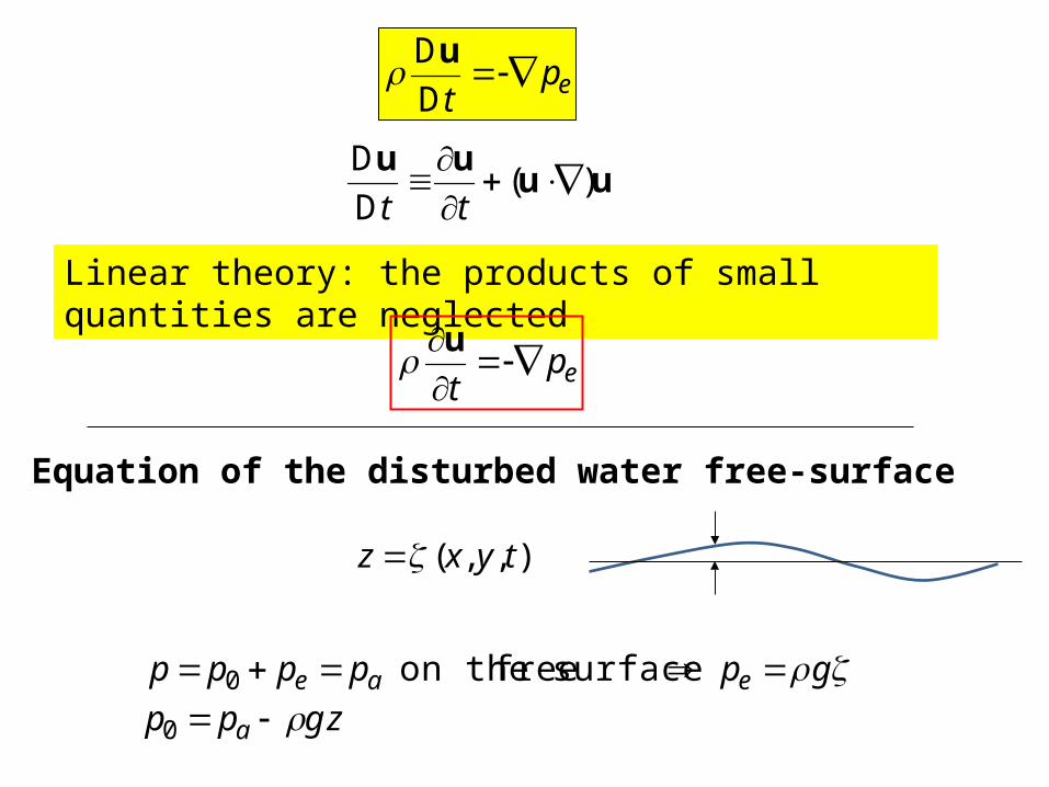
Euler’s equation (perfect fluid)

ept

D

Du

flow thefollowing derivativeD

D t

particle fluid ofon acceleratiD

D

t

u

ept

D

Du

uuuu

)(D

D

tt

Linear theory: the products of small quantities are neglected

ept

u

Equation of the disturbed water free-surface

),,( tyxz

gppppp eae surface free on the 0

zgpp a 0

gppppp eae surface free on the 0

ept

u

u tpe

),,( tyxz

gpe

g

t z

gt z

0

Kinematic boundary condition on the free surface

zztt

uD

D

0

zzt

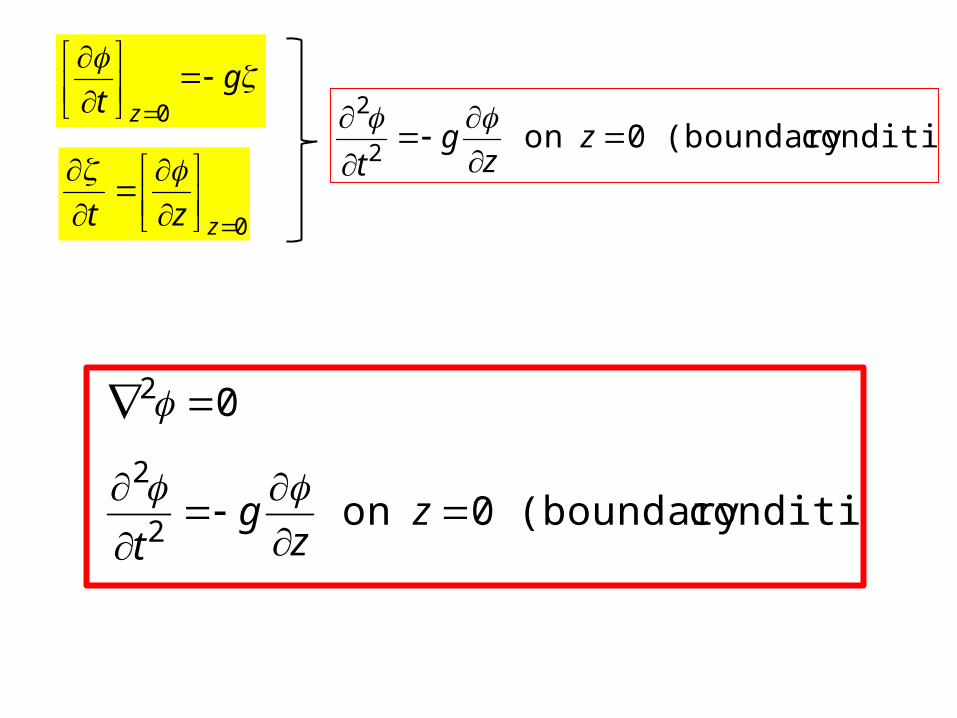
g

t z

0

0

zzt

condition)(boundary 0on

2

2

zz

gt

02

condition)(boundary 0on 2

2

zz

gt

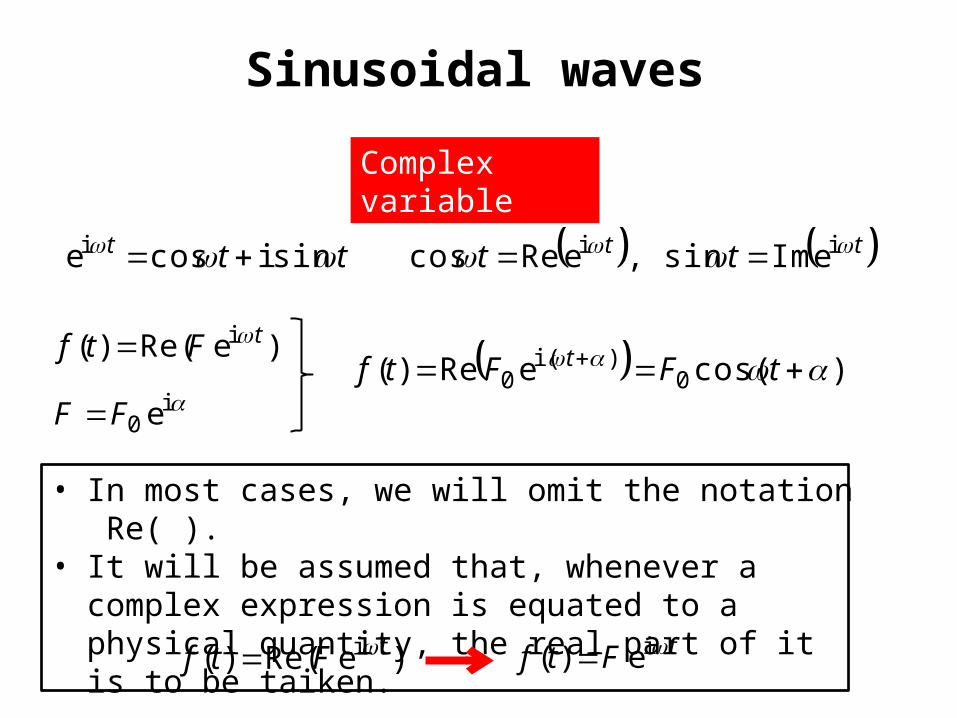
Sinusoidal waves

Complex variable

ttt sinicosei tt tt ii eImsin,eRecos

)eRe()( i tFtf

i0 eFF

)cos(eRe)( 0)i(

0 tFFtf t

• In most cases, we will omit the notation Re( ).• It will be assumed that, whenever a complex expression is

equated to a physical quantity, the real part of it is to be taiken.

)eRe()( i tFtf tFtf ie)(

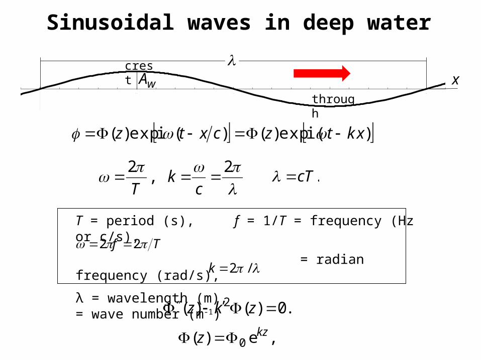
Sinusoidal waves in deep water

0. 5 1. 0 1. 5 2. 0

1. 0

0. 5

0. 5

1. 0

wA x

)i(exp)()(iexp)( xktzcxtz

2

,2

c

kT

.cT

.0)()( 2 zkz

,e)( 0kzz

T = period (s), f = 1/T = frequency (Hz or c/s),

= radian frequency (rad/s),

λ = wavelength (m), = wave number (m-1)

Tf 22

/2k

crest

through

)i(exp)()(iexp)( xktzcxtz

,e)( 0kzz

Sinusoidal waves in deep water

s9.13m/s6.21m300

s4.4m/s8.6m30

Tc

Tc

.2

2121

g

k

g

kcWave velocity

Dispersion relationship

0. 5 1. 0 1. 5 2. 0

1. 0

0. 5

0. 5

1. 0

wA x

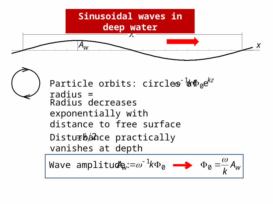
Sinusoidal waves in deep water

Particle orbits: circles of radius =

Wave amplitude: 01 kAw wA

k

0

kzk e01

Radius decreases exponentially with distance to free surface

Disturbance practically vanishes at depth 2

In deep water, the water particles have circular orbits.

The orbit radius decreases exponentially with the distance to the surface.

Sinusoidal waves in water of arbitrary, but uniform, depth h

)i(exp)()(iexp)( xktzcxtz

0. 5 1. 0 1. 5 2. 0

1. 0

0. 5

0. 5

1. 0

wA x

0)( h boundary condition at bottom

kzkzz ee)( 210)()( 2 zkz

khkh ee 21

)(cosh)( 0 hzkz

xxx eecosh21 xx

x

xx xx tanhcoshee

d

coshdsinh

21

0.0 0.5 1.0 1.5 2.00

1

2

3

4

x

xtanh

xsinh

xcosh

Sinusoidal waves in water of arbitrary, but uniform, depth h

0on 2

2

zz

gt

khgk tanh2

212

tanh2

hg

c

211 )tanh( khgkk

c

c

h

gc

tanh

Wave speed

Shallow water or long-wave limit: kh small khkh tanh

1for)( 21 khghc

Sinusoidal waves in water of arbitrary, but uniform, depth h

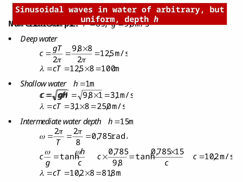
Numerical example: 8T s, 2m/s 8,9g

Deep water

m/s 5,122

88,9

2

gT

c

m 10085,12 cT

Shallow water 1h m

m/s 1,318,9 gHc

m/s 0,2581,3 cT

Intermediate water depth 15h m

rad/s 785,08

22

T

c

h

gc

tanh

cc

15785,0tanh

8,9

785,0 m/s 2,10c

m 8,8182,10 cT

Sinusoidal waves in water of arbitrary, but uniform, depth h

ghc

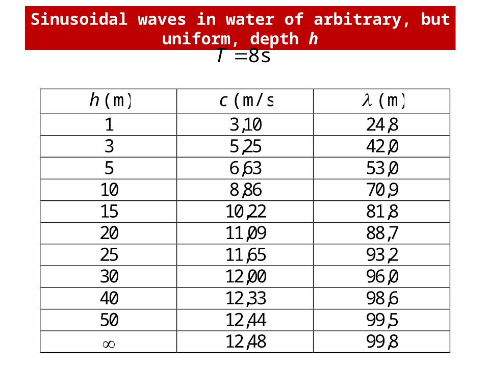
(m) h (m/s) c (m) 1 3,10 24,8 3 5,25 42,0 5 6,63 53,0

10 8,86 70,9 15 10,22 81,8 20 11,09 88,7 25 11,65 93,2 30 12,00 96,0 40 12,33 98,6 50 12,44 99,5 12,48 99,8

s8T

Sinusoidal waves in water of arbitrary, but uniform, depth h

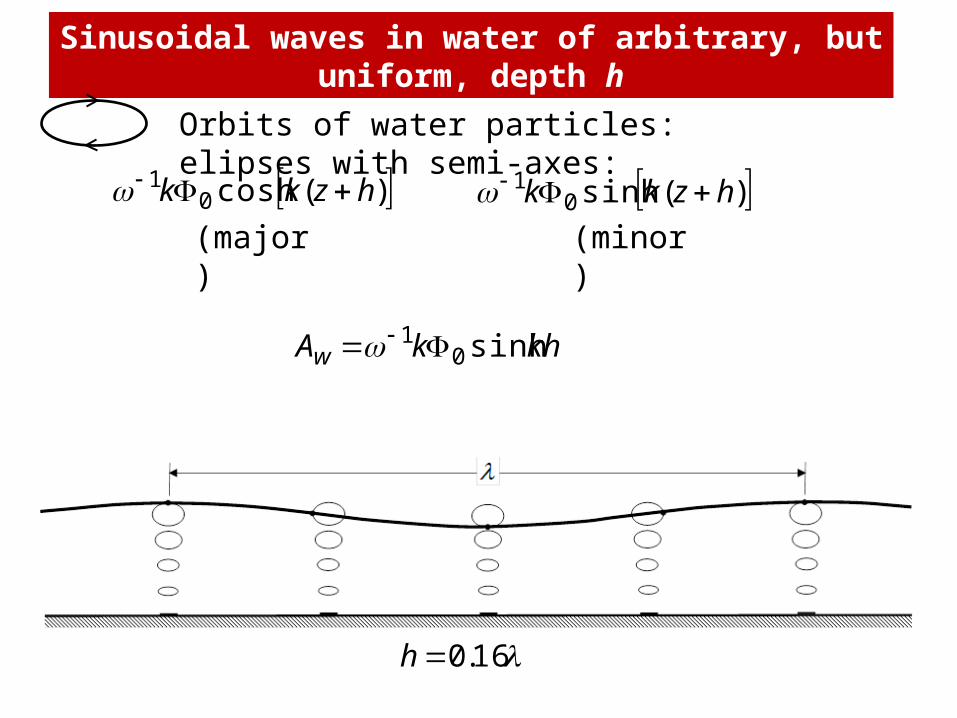
Sinusoidal waves in water of arbitrary, but uniform, depth h

Orbits of water particles: elipses with semi-axes:

)(cosh01 hzkk )(sinh0

1 hzkk (major) (minor)

khkAw sinh01

16.0h

wave crests

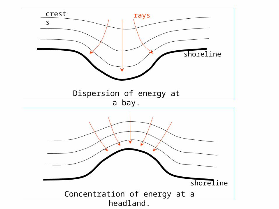
Refraction effects due to bottom bathymetry

The propagation velocity c decreases with decreasing depth h.

As the waves propagate in decreasing depth, their crests tend to become parallel to the shoreline

shoreline

rayscrests

shoreline

shoreline

Dispersion of energy at a bay.

Concentration of energy at a headland.

Standing waves. Reflection on a vertical wall

Standing waves. Reflection on a vertical wall

)(iexp)(,)(iexp)( 21 kxtzkxtz

kxzz tkxkxt cose)(2eee)( iiii1

tkxAtx w sincos2),(

kxzkx t sine)(2 i ...,2,1,0,at 0 nnkx

Horizontal velocity component:

Satisfies condition for reflection at vertical wall

antinodes nodes

Surface elevation

Wave energy and wave energy fluxUnlike wind, waves permit the transport of energy without the need for any net transport of material.

Kinetic energy (circular or elliptic orbits)

Potential energy (sea surface is not plane)

v

Potential energy per unit horizontal surface area (time averaged)

2potential 4

1wgAE

Kinetic energy per unit horizontal surface area (time averaged)

2kinetic 4

1wgAE

Total energy per unit horizontal surface area (time averaged, any water depth)

2kineticpotential 2

1wgAEEE

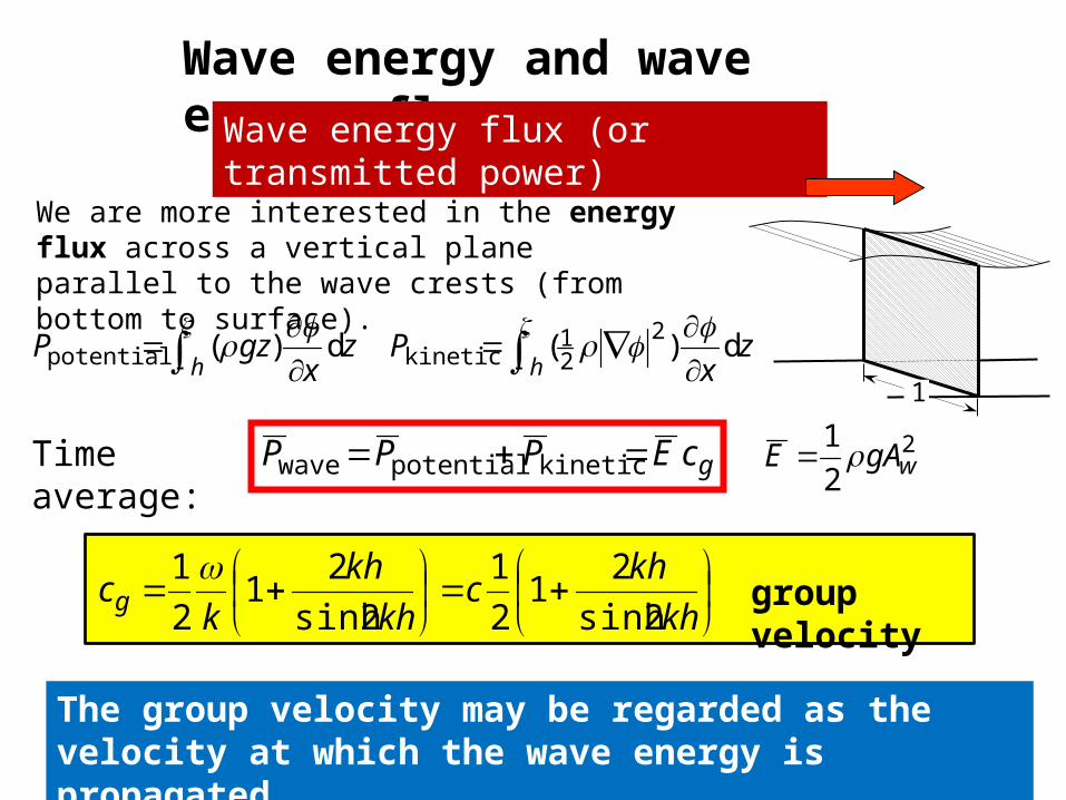
Wave energy and wave energy fluxWave energy flux (or transmitted power)

We are more interested in the energy flux across a vertical plane parallel to the wave crests (from bottom to surface).

1

h

zx

gzP d)(potential

h

zx

P d)(2

21

kinetic

gcEPPP kineticpotentialwaveTime average: 2

2

1wgAE

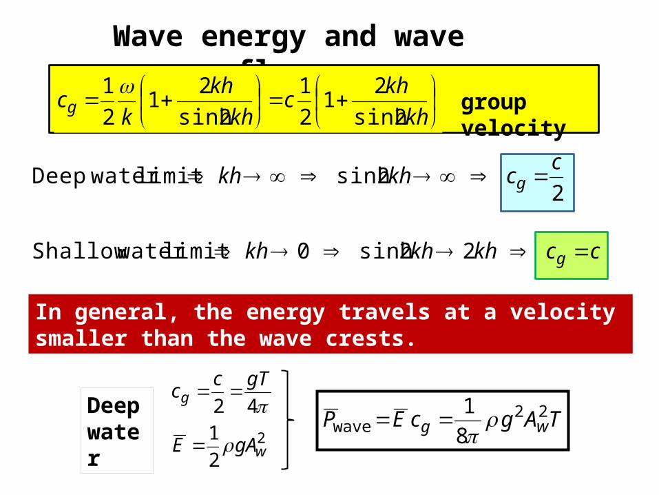
The group velocity may be regarded as the velocity at which the wave energy is propagated.

kh

khc

kh

kh

kcg 2sinh

21

2

1

2sinh

21

2

1 group velocity

Wave energy and wave energy flux

kh

khc

kh

kh

kcg 2sinh

21

2

1

2sinh

21

2

1 group velocity

2 2sinh limit water Deep

cckhkh g

cckhkhkh g 22sinh 0 limit water Shallow

In general, the energy travels at a velocity smaller than the wave crests.

Deep water 2

2

1wgAE

42

gTccg

TAgcEP wg22

wave 8

1

Exercise

)(tp

)(tp

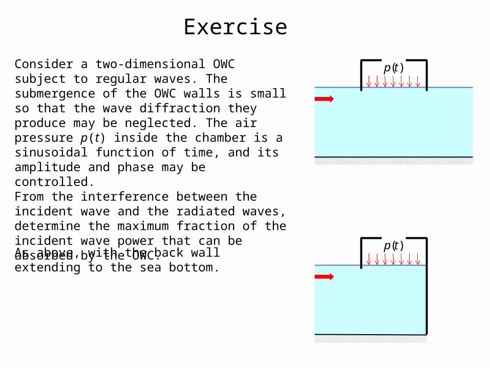
Consider a two-dimensional OWC subject to regular waves. The submergence of the OWC walls is small so that the wave diffraction they produce may be neglected. The air pressure p(t) inside the chamber is a sinusoidal function of time, and its amplitude and phase may be controlled.From the interference between the incident wave and the radiated waves, determine the maximum fraction of the incident wave power that can be absorbed by the OWC.

As above, with the back wall extending to the sea bottom.

Irregular waves

100 150 200 250 300ts

1

0.5

0

0.5

1

1.5m

Real ocean waves are not regular: they are irregular and random

Sea surface elevation at one location as a function of time

We want to describe the sea surface as a stochastic process, i.e. to characterize all possible observations (time records) that could have been made under the conditions of the actual observation.

An observation is thus formally treated as one realization of a stochastic process.

100 150 200 250 300ts

1

0.5

0

0.5

1

1.5

m

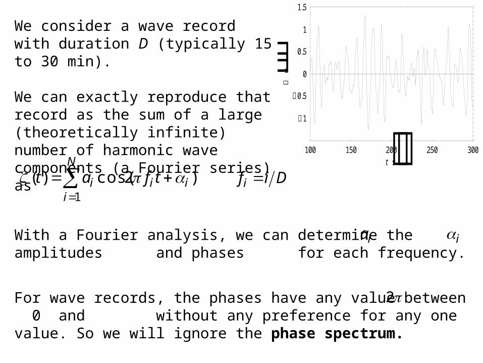
We consider a wave record with duration D (typically 15 to 30 min).

We can exactly reproduce that record as the sum of a large (theoretically infinite) number of harmonic wave components (a Fourier series) as

N

iiii tfat

1

),2cos()(

With a Fourier analysis, we can determine the amplitudes and phases for each frequency.

ia i

For wave records, the phases have any value between 0 and without any preference for any one value. So we will ignore the phase spectrum.

2

Difi

Only the amplitude spectrum remains to characterize the wave record.

To remove the sample character of the spectrum, we should repeat the experiment many times (M) and take the average over all these experiments, to find the average amplitude spectrum

i

M

mmii fa

Ma sfrequencie allfor

1

1,

However, it is more meaningful to use the variance

of each wave component . An important reason is that the wave energy is proportional to the square of the wave amplitude (not to the amplitude).

M

mmii a

Ma

1

2,2

1221 1

The variance spectrum is discrete, i.e., only the frequencies are present, whereas in fact all frequencies are present at sea.

This is resolved by letting the frequency interval .

The variance density spectrum is defined as

Difi

.01 Df

221

0

1lim)( if

f af

fS

Units for are or )( fS f sm2 /Hzm2

0.05 0.10 0.15 0.20 0.25

1

2

3

4

(Hz) Frequency f

Typical variance density spectrum

The variance density spectrum gives a complete description of the surface elevation of ocean waves in statistical sense, provided that the surface elevation can be seen as a stationary Gaussian process.

To use this approach, a wave record needs to be divided into segments that are each assumed to be approximately stationary (a duration of about 30 min is commonly used).

The sea surface elevation is a random function of time. Its total variance is

0

2 d)( ffS f

We recall that the time-averaged total (potential plus kinetic energy) of a regular wave per unit horizontal surface is

If we multiply by we obtain the energy density spectrum

221

wgAE

)( fS f g

.1

lim)()( 2

021

if

ff af

gfgSfE

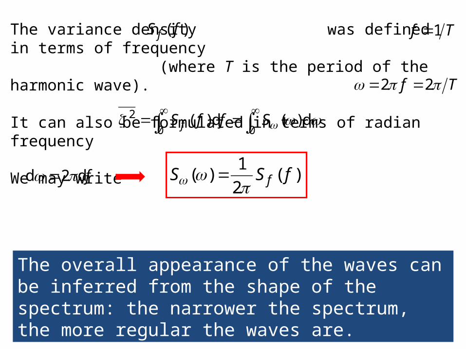
The variance density was defined in terms of frequency (where T is the period of the harmonic wave).

It can also be formulated in terms of radian frequency

We may write

Tf 1)( fS f

Tf 22

00

2 d)(d)( SffS f

).(2

1)( fSS f

fd2d

The overall appearance of the waves can be inferred from the shape of the spectrum: the narrower the spectrum, the more regular the waves are.

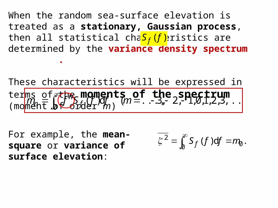
When the random sea-surface elevation is treated as a stationary, Gaussian process, then all statistical characteristics are determined by the variance density spectrum .

These characteristics will be expressed in terms of the moments of the spectrum (moment of order m)

)( fS f

,...).3,2,1,0,1,2,3...,(d)(0

mffSfm fn

n

For example, the mean-square or variance of surface elevation: .d)( 00

2 mffS f

Significant wave height and mean wave period

The significant wave height is the mean value of the highest one-third of wave heights in the wave record.

sH

It is given approximately by 00 4 mHH ms

Several different definitions of “mean” period for irregular waves are used.

One is the peak period

Another is the energy period

pp fT 1

pf

0

1

m

mTe

The characteristics of the frequency spectra of sea waves have been fairly well established through analyses of a large number of wave records taken in various oceans and seas.

The spectra of fully developed waves in deep water can be approximated by the Pierson-Moskowitz equation

4542 )(675.0exp1688.0)( fTfTHfS eesf

4542 )(1052exp6.262)( ees TTHS

ExerciseEstablish a relationship between the peak period and the energy period for the Pierson-Mokowitz spectrum.

In regular waves:• energy per unit horizontal surface area

• energy flux per unit wave crest length

• In deep water

221

wgAE

Energy flux of irregular waves

gcEP wave

.)4(21 fgccg

In irregular waves:• In

• By integration

)d,( fff

ff

fSg

ffSgcffEcP ffgfg d1

)(4

d)(d)(d2

wave

1

2

0

2

wave 4d

1)(

4

mg

ff

fSg

P f

01 mmTe

04 mHs .

642

2

wave es THg

P

irregular waves

2sm8.9 g

3mkg1025 es THP 2wave 490.0

kW/m inwaveP

m in sH

s in eT

1

2

wave 4 mg

P

Wave climateSo far, the statistical characteristics of the waves were considered for short term, stationary conditions, usually for the duration of a wave record (15 to 30 min).

• For long-term statistics, over durations of several years (possibly tens of years) the conditions are not stationary.

• For these long time scales, each stationary condition (with a duration of 15 to 30 min) is replaced with its values of the significant wave height and period. This gives a long-term sequence of these values with a time interval of typically 3 h, which can be analysed to estimate the long-term statistical characteristics of the waves.

• The number of observations in then presented (instead of the probability density) in bins of size ),( es TH

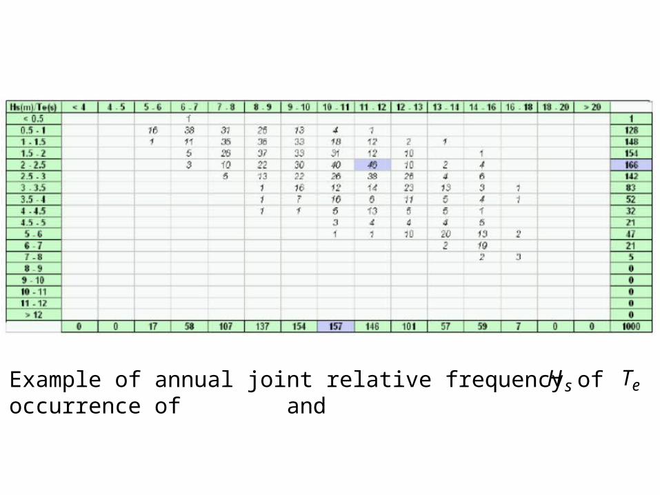
Example of annual joint relative frequency of occurrence of and sH eT

END OF PART 2LINEAR THEORY OF OCEAN

SURFACE WAVES