SPE-169640

The Use of Computational Fluid Dynamics to Troubles hoot Excessive Metal Loss in a Carbon Steel Flowline: A Case History Eugenia Marinou, Valdir de Souza, Lesmana Djayapertapa, Ken Watson, Senergy Ltd; Craig Moor, Frances Chalmers, Centrica UK

Copyright 2014, Society of Petroleum Engineers This paper was prepared for presentation at the SPE International Oilfield Corrosion Conference and Exhibition held in Aberdeen, United Kingdom, 12–13 May 2014. This paper was selected for presentation by an SPE program committee following review of information contained in an abstract submitted by the author(s). Contents of the paper have not been reviewed by the Society of Petroleum Engineers and are subject to correction by the author(s). The material does not necessarily reflect any position of the Society of Petroleum Engineers, its officers, or members. Electronic reproduction, distribution, or storage of any part of this paper without the written consent of the Society of Petroleum Engineers is prohibited. Permission to reproduce in print is restricted to an abstract of not more than 300 words; illustrations may not be copied. The abstract must contain conspicuous acknowledgment of SPE copyright.

Abstract Greater Kittiwake Area (GKA) well KA-15, while not a significant oil producer anymore, provides large amounts of hot produced water which assists the field’s first stage separation process. Historically, there have been numerous records of significant metal loss in the carbon steel flowline, especially at bends and welds, attributed to the line’s convoluted configuration, flow rates and associated potential for erosion-corrosion effects. This paper outlines the investigation process and corresponding findings. For fluid velocity calculations, computational fluid dynamics (CFD) was employed to allow highly accurate determination of the fluid velocity profile as well as the magnitude of localised wall shear stress. This was so as to assess the efficiency of the applied corrosion inhibitor and to provide a means of well management to avoid exceeding erosional velocities. In addition, a thorough review of the input parameters used for the corrosion inhibitor selection was performed; this revealed that erroneous inputs and inadequate testing were used for laboratory qualification of the chemical, with detrimental consequences for the flowline’s integrity. The study eventually concluded that the original material selection for the flowline was not appropriate for at least the current operating conditions and chemical testing was performed on unverified assumptions. This highlights the importance of using accurate methodology to validate inputs and that of periodic in-depth system reviews to ensure that new field parameters are re-evaluated correctly. Introduction The flowline associated with producing well KA-15 in the Greater Kittiwake Area has been historically prone to spool change-outs, caused by excessive metal loss as verified by regular inspections. The 4″ line is made of carbon steel and spans the distance from the wellhead to the separator through what is described as a “convoluted” path with a lot of bends and drops from height. The line is seven years old (installed in 2006 to replace the previous flowline). The examination report of the latter highlighted some corrosion on the welds. Currently the flowline transports produced fluids at 97 °C with an approximate watercut of 95% and is treated continuously with a corrosion inhibitor at concentrations typically around 50 ppm, although higher injection rates have also been attempted to try and arrest the high corrosion rates measured. This paper discusses the investigation conducted to identify the possible causes of the high wall loss detected by the inspections and advise on suitable mitigation measures going forward. To this end, the review performed concentrated on evaluating the following aspects initially independently and eventually through establishing interrelated factors that may have preferentially influenced the observed outcome:

• Inspection data between years 2008-2012;

2 SPE 169640

• Corrosion monitoring data (between 2010-2011 for the corrosion coupon and September 2012 to February 2013 for the corrosion probe);

• Review of well test data to ensure that the velocities used for chemical testing were compatible with the flowing regime in place;

• Calculation of flow velocities and wall shear rates in sensitive parts of the system using a range of recent well test data to simulate high/low flowrates, using computational fluid dynamics (CFD) analysis. The results were then compared with accepted velocity limits for the material;

• Review of chemical qualification testing and application history; and

• Review of the examination report for the replaced flowline in 2006.

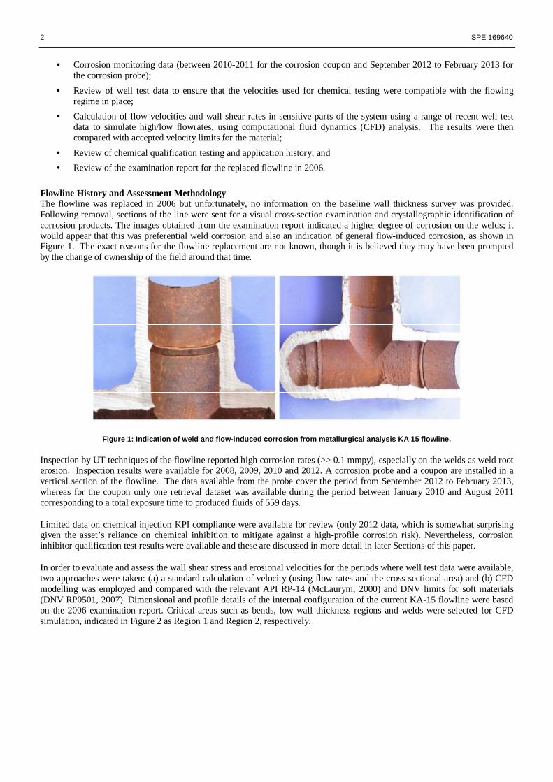
Flowline History and Assessment Methodology The flowline was replaced in 2006 but unfortunately, no information on the baseline wall thickness survey was provided. Following removal, sections of the line were sent for a visual cross-section examination and crystallographic identification of corrosion products. The images obtained from the examination report indicated a higher degree of corrosion on the welds; it would appear that this was preferential weld corrosion and also an indication of general flow-induced corrosion, as shown in Figure 1. The exact reasons for the flowline replacement are not known, though it is believed they may have been prompted by the change of ownership of the field around that time.

Figure 1: Indication of weld and flow-induced corro sion from metallurgical analysis KA 15 flowline.

Inspection by UT techniques of the flowline reported high corrosion rates (>> 0.1 mmpy), especially on the welds as weld root erosion. Inspection results were available for 2008, 2009, 2010 and 2012. A corrosion probe and a coupon are installed in a vertical section of the flowline. The data available from the probe cover the period from September 2012 to February 2013, whereas for the coupon only one retrieval dataset was available during the period between January 2010 and August 2011 corresponding to a total exposure time to produced fluids of 559 days.

Limited data on chemical injection KPI compliance were available for review (only 2012 data, which is somewhat surprising given the asset’s reliance on chemical inhibition to mitigate against a high-profile corrosion risk). Nevertheless, corrosion inhibitor qualification test results were available and these are discussed in more detail in later Sections of this paper.

In order to evaluate and assess the wall shear stress and erosional velocities for the periods where well test data were available, two approaches were taken: (a) a standard calculation of velocity (using flow rates and the cross-sectional area) and (b) CFD modelling was employed and compared with the relevant API RP-14 (McLaurym, 2000) and DNV limits for soft materials (DNV RP0501, 2007). Dimensional and profile details of the internal configuration of the current KA-15 flowline were based on the 2006 examination report. Critical areas such as bends, low wall thickness regions and welds were selected for CFD simulation, indicated in Figure 2 as Region 1 and Region 2, respectively.

SPE 169640 3

Figure 2: Pipework region selection for CFD modelli ng.

The assessment focussed on the expected degradation mechanisms for the flowline, which for carbon steel are as follows:

• CO2 corrosion (efficiency of the corrosion inhibitor dosage and its availability);

• Erosion-corrosion or flow-induced corrosion;

• MIC corrosion (unlikely due to the high reservoir temperature);

• Cracking mechanisms due to H2S (not assessed as the material specification was not available, but the material may be required to comply with ANSI/NACE (MR0175/ ISO15156, 2010) for sour service, as the produced fluids contain H2S).

Sand presence in the system has not been reported in the field to-date and, therefore, in this case the system was considered to be solids-free. Also, the chemical composition of the welds was not known and these have not been discussed in this paper.

Results and Discussion

Inspection and Corrosion Monitoring: Wall thickness measurements performed by UT showed values of wall loss that were much higher than the acceptable 0.1 mmpy for carbon steel. The line has been inspected every year since 2008 at different locations. KA-15 is a 4″ line with a nominal wall thickness of 20 mm and a 6 mm corrosion allowance (CA). There is no information available on the initial wall thickness (baseline survey) of the flowline when installed in 2006. The first available inspection results in 2008 indicated the wall thickness to be between 14.3 to 23.5 mm.

The CA of 6 mm would allow for a 0.3 mmpy corrosion rate for an expected design life of 20 years. However, there are two issues with this statement:

• The design life of 20 years is not certain but has been suggested by the Operator as a reasonable assumption;

• The corrosion rate of 0.3 mmpy is not supported by any documented reference.

For this reason and in the absence of the formal documentation and information on the parameters used for the initial material selection for the line, all further assessments were conducted on the premise of a maximum inhibited annual corrosion rate of 0.1 mmpy.

A summary of the inspection results for the areas with measured wall thickness which resulted in corrosion rates higher than 0.1 mmpy is shown in Table 1.

4 SPE 169640

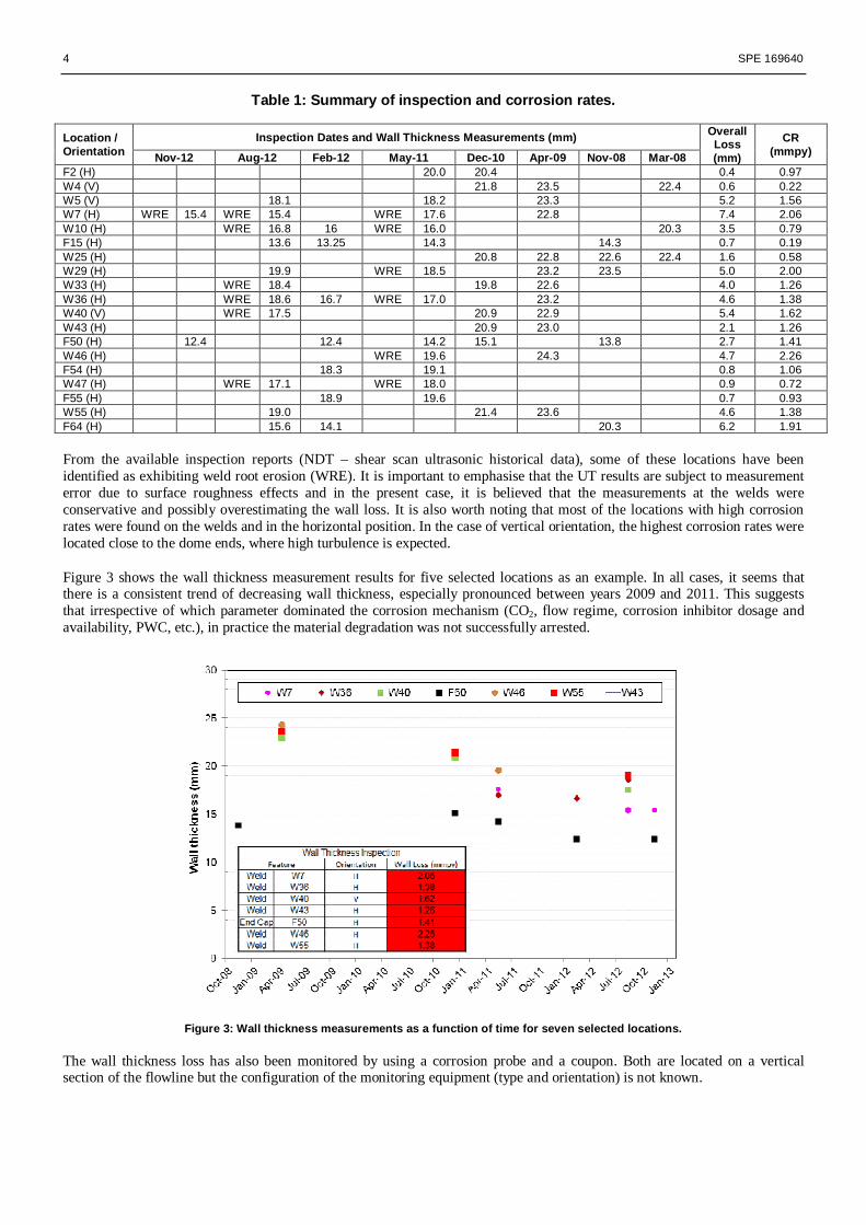
Table 1: Summary of inspection and corrosion rates.

Location / Orientation

Inspection Dates and Wall Thickness Measurements (m m) Overall Loss (mm)

CR (mmpy) Nov-12 Aug-12 Feb-12 May-11 Dec-10 Apr-09 Nov-08 Ma r-08

F2 (H) 20.0 20.4 0.4 0.97 W4 (V) 21.8 23.5 22.4 0.6 0.22 W5 (V) 18.1 18.2 23.3 5.2 1.56 W7 (H) WRE 15.4 WRE 15.4 WRE 17.6 22.8 7.4 2.06 W10 (H) WRE 16.8 16 WRE 16.0 20.3 3.5 0.79 F15 (H) 13.6 13.25 14.3 14.3 0.7 0.19 W25 (H) 20.8 22.8 22.6 22.4 1.6 0.58 W29 (H) 19.9 WRE 18.5 23.2 23.5 5.0 2.00 W33 (H) WRE 18.4 19.8 22.6 4.0 1.26 W36 (H) WRE 18.6 16.7 WRE 17.0 23.2 4.6 1.38 W40 (V) WRE 17.5 20.9 22.9 5.4 1.62 W43 (H) 20.9 23.0 2.1 1.26 F50 (H) 12.4 12.4 14.2 15.1 13.8 2.7 1.41 W46 (H) WRE 19.6 24.3 4.7 2.26 F54 (H) 18.3 19.1 0.8 1.06 W47 (H) WRE 17.1 WRE 18.0 0.9 0.72 F55 (H) 18.9 19.6 0.7 0.93 W55 (H) 19.0 21.4 23.6 4.6 1.38 F64 (H) 15.6 14.1 20.3 6.2 1.91

From the available inspection reports (NDT – shear scan ultrasonic historical data), some of these locations have been identified as exhibiting weld root erosion (WRE). It is important to emphasise that the UT results are subject to measurement error due to surface roughness effects and in the present case, it is believed that the measurements at the welds were conservative and possibly overestimating the wall loss. It is also worth noting that most of the locations with high corrosion rates were found on the welds and in the horizontal position. In the case of vertical orientation, the highest corrosion rates were located close to the dome ends, where high turbulence is expected.

Figure 3 shows the wall thickness measurement results for five selected locations as an example. In all cases, it seems that there is a consistent trend of decreasing wall thickness, especially pronounced between years 2009 and 2011. This suggests that irrespective of which parameter dominated the corrosion mechanism (CO2, flow regime, corrosion inhibitor dosage and availability, PWC, etc.), in practice the material degradation was not successfully arrested.

Figure 3: Wall thickness measurements as a function of time for seven selected locations.

The wall thickness loss has also been monitored by using a corrosion probe and a coupon. Both are located on a vertical section of the flowline but the configuration of the monitoring equipment (type and orientation) is not known.

SPE 169640 5

It is understood that historical corrosion monitoring data are only available for the time periods as follows:

• For the corrosion coupon: from 30-Jan-2010 until 12-Aug-2011; there is no information as to whether a new coupon was installed in the line after the last recorded retrieval.

• For the corrosion probe: the provided information indicated that a new logger and T80 ER probe were installed in August of 2012 with monitoring from September 2012 to February 2013; there is no information regarding an earlier probe in the line or the status of the probe post-March 2013 (records indicate that the probe expired at that time).

The corrosion coupon retrieved in 2011 and covering the time period between January 2010 and August 2011 (559 days) showed 0.041 mmpy of general corrosion and 0.072 mmpy for pitting. These values are considered low according to NACE (RP0775, 2005), however, it is important to emphasise that the coupon is located in a suboptimal part of the system, as the majority of the observed high metal loss has been found in horizontal sections.

The corrosion probe readings from September 2012 to February 2013 resulted in an average corrosion rate of 0.7 mmpy (±0.1). The corrosion probe is also located in a vertical section of the flowline close to the coupon so similar considerations to those outlined above apply. As mentioned, the probe expired in March 2013 and no further readings have since been available.

Despite the limitations originating from the position of the corrosion probe, the corrosion rate measured appears to indicate that unacceptable corrosion is taking place and that would corroborate the historical NDT findings. This investigation also assessed the impact of high liquid flow rates (from well test data); again, the corrosion rate appears to increase as a function of higher fluid velocities (Figure 4).

Figure 4: Probe readings and well test data for the case designated ‘high flow’ rate.

CFD Modelling and System Velocities: Computational Fluids Dynamics (CFD), in its simple term, is a computational method used to model and simulate fluid flow in a bounded domain. The bounded domain is needed to generate what is known as the ‘volume mesh’ where the fluid would flow. The fluid simulated could be of any type, such as liquids (e.g. water, oil), gas (e.g. air, nitrogen, methane), or particles (e.g. sand). The combination of multiple fluids, known as multiphase flow, can also be simulated, e.g., water, oil and gas, or water with sand which leads to erosion analysis.

Behind the scenes of CFD is simple physics; the motion of a fluid element in a three dimensional space is described by the continuity, momentum and energy equations and the governing mathematical equations are solved numerically using computers, hence the term Computational. CFD is a powerful technique and a proven technology, particularly in the aerospace and automotive industries. CFD has been used regularly and aggressively as a design tool, troubleshooting tool, or as a means to understand what happens with the dynamics of the fluids. Conventional velocity modelling of flow in pipes assumes uniform flow for the cross sectional area. Whilst this may be true for some flow in straight pipelines it is certainly not the case where there are bends and tortuosity in more convoluted flow lines. The CFD approach is rigorous in that the geometry of the

0

0.1

0.2

0.3

0.4

0.5

0.6

0.7

0.8

0.9

1

Sep-12 Oct-12 Nov-12 Dec-12 Jan-13 Feb-13

Cor

rosi

on r

ate

(mm

py)

High flow rate

14488 bpd-

Well Test

Probe Readings - Corrosion Rates (mmpy)

6 SPE 169640

pipes is honoured together with the fluid properties, rates and dynamics giving a true picture of velocity maxima and minima across the entire system. This velocity fluctuation can lead to poor inhibitor retention, increased corrosion and increased erosion at high velocity regions of the system. The impact of the increased velocity needs to be considered along with the area subject to this velocity.

Therefore, given the complexity of the flowline’s geometry in the present case (especially around bends) and as standard flowrate/pipe diameter calculations would inevitably provide only bulk, average liquid velocities, it was decided that CFD would be the best available modelling approach to obtain highly accurate flow velocities and wall shear stress profiles.

Flow parameters and well test data

Flow conditions were derived using well test data. The modelling approach taken in this study attempted to represent two different flow rate regimes for the line, a “low flow” at ca. 9,000 bpd and a “high flow” one at ca. 15,000 bpd. This was to ascertain the KA-15-specific threshold above which flow effects may become too significant for chemical inhibition to be successful. As the watercut is high, the fluid through the flowline was assumed to be only water with a temperature of 97 °C. The outlet conditions were assumed to be comparable and hence match those of the inlet.

Geometry configuration and selected sections

The external geometry was based on the as-built isometrics. Two regions (sections) of the KA-15 flowline were initially chosen to perform CFD analysis as illustrated in Figure 2. These regions represent areas with high wall loss (>>0.1 mmpy) on the dome ends and also weld root erosion from the inspection results. The boundaries of Region 1 cover the length between the wellhead to a dome-end feature; this was chosen because the fluid velocity would be at its maximum in the flowline (prior to frictional pressure losses further downstream). Region 2 was selected to cover a number of locations with a high measured wall thickness loss. Figure 5 shows an example of the CFD preparation for modelling the external geometry using specialised 3D graphics software.

Figure 5: Example of an original Isometric drawing and the external geometry preparation for CFD model ling.

The following assumptions were made for the CFD simulations:

• Pipe wall thickness 15 mm throughout; this was selected based on the last inspection results for the dome ends and so as to represent current pipeline flowing conditions and simplify the geometry for the CFD modelling. According to this, the fluid O.D. is 84.3 mm;

• Added the butt weld feature on each Tee; this weld protrudes into the bore by 6 mm; • Added 500 mm to the inlet, so there is approximately 1,000 mm straight at both the inlet and outlet end of each

region;

SPE 169640 7

• The flowing fluid was assumed to be only water (and since the watercut is 95%).

CFD simulation results

CFD simulations were performed for Regions 1 and 2 for the high/low water flow rates. To facilitate the interpretation of the results (influence of geometrical configuration and analysis of velocity and wall shear stress), ‘corners' or bends were designated for each region. For simplicity, only the high flow rate results for Region 1 are described in detail and depicted pictorially in this paper, as these represent the worst-case conditions for the system.

The velocity and shear stress profiles modelled for Region 1 are shown in Figure 6 (a-b). The velocity reaches values higher than 10 m/s in dome ends (the “red” regions) especially on the weld locations. In (b), the areas in “red” highlight high values of shear stresses in agreement with the velocity profile, and reach a magnitude in excess of 200 Pa. In terms of the corner profiles, (c) and (d) show a close-up image of the velocity and shear stress profile for Corner 3 emphasising high shear stress areas. Similar results were obtained when modelling Region 2.

Figure 6: Velocity and wall shear stress profiles f or pipework designated “Region 1” for a high flow r ate.

It is worth noting that performing standard fluid velocity calculations for the ‘low/high’ cases, gave average velocities of 2.8 and 4.7 m/s (assuming a 15 mm wall thickness), respectively, i.e., if CFD had not been used for this assessment, the impact of flow-related effects on the overall corrosivity would have been missed.

The CFD simulations also identified areas of excessive shear rates, i.e., in the order of a few thousands of Pa. These are the result of localised ‘wavelets’ of hydrodynamic energy and were found in regions around all the welds. Figure 7 ‘zooms’ into such a section to highlight the location and extent of these regions.

8 SPE 169640

Figure 7: Velocity and wall shear stress profiles f or pipework designated “Region 1” for a high flow r ate. The length of the “red” area spans ca. 8 mm.

A summary of the maximum velocity and maximum shear stress for each region under high and low flow conditions obtained through CFD is shown in Table 2. The velocity can reach values of 11.6 m/s and shear stress of 3,156 Pa under high flow conditions and 7 m/s velocity and 1,316 Pa shear stress under low flow conditions. These values are very high and are expected to affect the corrosion inhibitor’s ability to form a homogeneous protective film on a metal surface, which is discussed in more detail later in this paper.

Table 2: Summary of the maximum velocity and maximu m shear stress for high and low flow conditions.

Flow (bpd) Standard Velocity Calculation (m/s) (1) Region Vmax (m/s)

Average WSS (Pa) (2) Max WSS (Pa)

Flat area Weld

Low 2.8 1 6.5 61.9 203.8 525

2 7.0 60.5 197.4 1,316

High 4.7 1 10.8 169.7 556.1 1,298

2 11.6 164.6 545.5 3,156

Notes: (1) Calculation based on the expression: velocity = flow-rate/cross-sectional area. The wall thickness used for calculating the ID of the pipe was 15 mm. (2) Example for one of the corners for each region at low and high flow rate.

The velocity of 11.6 m/s is above the maximum of 10 m/s for soft materials (DNV-RP0501, 2007) and also the limits established by API RP 14E of 6 m/s (McLaurym, 2000). Although the DNV-RP0501 does not state a velocity limit specifically for steel, the 10 m/s was used as the reference limit in this paper.

On this basis, the low flow rate modelled scenario did not lead to erosional velocities; however, the high flow rate exceeded the 10 m/s limit. The CFD modelling performed here has highlighted high calculated values of velocities and shear stresses at the dome ends which suggests a good correlation with the UT inspection results and the findings of the 2006 examination report and implied WRE and PWC in a number of areas. It should be stressed that irrespective of flow rate (high/low), the inherent corrosivity of the fluid is such that velocity-related effects serve primarily to accelerate corrosion and compromise the inhibitor’s ability to form a uniform protective layer, as discussed in the Section on chemical selection. What this means in practice is that there are synergistic effects into play, with the erosional velocity being a contributing factor rather than the dominant material degradation mechanism.

Chemical Mitigation and Qualification Testing From the records available it appears that the flowline has been historically treated with a corrosion inhibitor, at least from 2010 onwards. Between 2010 and Q2 of 2011, a combined scale/corrosion inhibitor (Product “A”) was injected into the KA-15 flowline at 50 ppm on total fluids to begin with based on produced water rates, though later lowered to 15 ppm for a period in response to deteriorating oil-in-water/separation issues. The asset changed out this chemical to another combined scale/corrosion inhibitor (Product “B”), with an improved environmental profile. The injection rate was then set to 50 ppm.

SPE 169640 9

However, the corrosion rates as measured by the corrosion probe continued to be unacceptable despite the good compliance with the injection rate KPI, at least in 2012 which is the only year for which data were readily available for review (Figure 8).

As expected, the asset’s first response was to increase the injection dosage of the chemical and continue to monitor metal loss readings. Despite a significant increase in injection rate, the measured corrosion rates remained unacceptable, hence why additional factors had to be assessed, especially around the laboratory testing parameters for the chemical qualification, flow regime in the flowline and the tolerance of the carbon steel metallurgy to the in situ corrosive environment.

Figure 8: Corrosion inhibitor KPI compliance in 201 2.

Chemical qualification parameters: The review conducted brought to light a number of findings regarding the chemical qualification testing:

• It seems that no testing on pipe welds has ever taken place, at least not for the two most recent chemical changes (Products “A” and “B”). This is surprising and not in compliance with standard corrosion inhibitor selection criteria, especially given the indications of pipe weld corrosion from the 2006 examination report.

• The dosage established for Product “A” was based on the flowing conditions of another subsea tieback in the wider field (Goosander):

o Temperature = 70 °C o CO2 partial pressure = 0.69 bar o Linear velocity = 0.65 m/s (or 1,050 rpm)

These parameters, however, are not representative of the KA-15 flowline conditions, as will be discussed further in this Section. It would appear that an empirical extrapolation took place to derive the 50 ppm injection rate without validation of conditions so as to reflect the different flowing environment.

When Product “A” was replaced by Product “B”, laboratory testing specific to KA-15 was conducted. For the RCE testing at least, which is the most representative of a flowing system, the following input parameters were used:

o Temperature = 70 °C o CO2 partial pressure = 0.53 bar o Linear velocity = 1.24 m/s (or 2,000 rpm)

10 SPE 169640

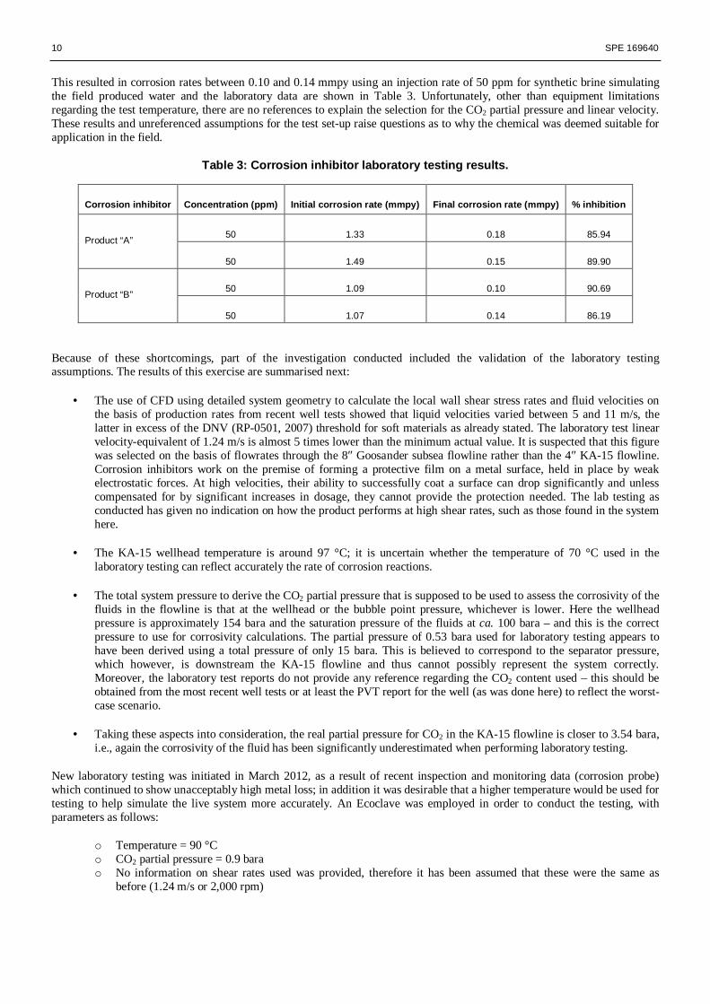
This resulted in corrosion rates between 0.10 and 0.14 mmpy using an injection rate of 50 ppm for synthetic brine simulating the field produced water and the laboratory data are shown in Table 3. Unfortunately, other than equipment limitations regarding the test temperature, there are no references to explain the selection for the CO2 partial pressure and linear velocity. These results and unreferenced assumptions for the test set-up raise questions as to why the chemical was deemed suitable for application in the field.

Table 3: Corrosion inhibitor laboratory testing res ults.

Corrosion inhibitor Concentration (ppm) Initial cor rosion rate (mmpy) Final corrosion rate (mmpy) % in hibition

Product “A” 50 1.33 0.18 85.94

50 1.49 0.15 89.90

Product “B” 50 1.09 0.10 90.69

50 1.07 0.14 86.19

Because of these shortcomings, part of the investigation conducted included the validation of the laboratory testing assumptions. The results of this exercise are summarised next:

• The use of CFD using detailed system geometry to calculate the local wall shear stress rates and fluid velocities on the basis of production rates from recent well tests showed that liquid velocities varied between 5 and 11 m/s, the latter in excess of the DNV (RP-0501, 2007) threshold for soft materials as already stated. The laboratory test linear velocity-equivalent of 1.24 m/s is almost 5 times lower than the minimum actual value. It is suspected that this figure was selected on the basis of flowrates through the 8″ Goosander subsea flowline rather than the 4″ KA-15 flowline. Corrosion inhibitors work on the premise of forming a protective film on a metal surface, held in place by weak electrostatic forces. At high velocities, their ability to successfully coat a surface can drop significantly and unless compensated for by significant increases in dosage, they cannot provide the protection needed. The lab testing as conducted has given no indication on how the product performs at high shear rates, such as those found in the system here.

• The KA-15 wellhead temperature is around 97 °C; it is uncertain whether the temperature of 70 °C used in the laboratory testing can reflect accurately the rate of corrosion reactions.

• The total system pressure to derive the CO2 partial pressure that is supposed to be used to assess the corrosivity of the fluids in the flowline is that at the wellhead or the bubble point pressure, whichever is lower. Here the wellhead pressure is approximately 154 bara and the saturation pressure of the fluids at ca. 100 bara – and this is the correct pressure to use for corrosivity calculations. The partial pressure of 0.53 bara used for laboratory testing appears to have been derived using a total pressure of only 15 bara. This is believed to correspond to the separator pressure, which however, is downstream the KA-15 flowline and thus cannot possibly represent the system correctly. Moreover, the laboratory test reports do not provide any reference regarding the CO2 content used – this should be obtained from the most recent well tests or at least the PVT report for the well (as was done here) to reflect the worst-case scenario.

• Taking these aspects into consideration, the real partial pressure for CO2 in the KA-15 flowline is closer to 3.54 bara, i.e., again the corrosivity of the fluid has been significantly underestimated when performing laboratory testing.

New laboratory testing was initiated in March 2012, as a result of recent inspection and monitoring data (corrosion probe) which continued to show unacceptably high metal loss; in addition it was desirable that a higher temperature would be used for testing to help simulate the live system more accurately. An Ecoclave was employed in order to conduct the testing, with parameters as follows:

o Temperature = 90 °C o CO2 partial pressure = 0.9 bara o No information on shear rates used was provided, therefore it has been assumed that these were the same as

before (1.24 m/s or 2,000 rpm)

SPE 169640 11

As can be seen, while the temperature chosen is much closer to the system’s at 97 °C, again the partial pressure of CO2 is much lower than the actual 3.54 bara, therefore, the lab tests are still not representative of the conditions in the KA-15 flowline. Perhaps not unexpectedly, the chemical failed to confer the required inhibition (1.58 mmpy as shown in Table 4) at a dosage of 50 ppm but more alarmingly at conditions that are far less corrosive than those in the field. The vendor’s recommendation in response to the high corrosion probe readings was to keep increasing the chemical injection rate in increments of 25 ppm, measure chemical residuals in the laboratory and try to correlate with the readings of the corrosion probe; this also failed to arrest the corrosion rate and had to be suspended because of its detrimental impact on oil-in-water concentration.

Table 4: Measured corrosion rates for Product “B” u sing an Ecoclave.

Product “B” dosage (ppm)

Initial corrosion rate (mmpy)

Final corrosion rate (mmpy)

% Inhibition

50 11.52 1.58 86.28

Further to the cost associated with chemical injection at high concentration rates, it is important to highlight the significance of providing and sense-checking the input parameters for the design of the testing set-up. To appreciate the impact of using erroneous data in the present case, some theoretical corrosion rate calculations were performed using different industry-accepted models to represent (a) the chemical vendor’s inputs for the laboratory testing and qualification of the corrosion inhibitor, i.e., a pressure of 15 bara, temperature of 70 °C, a brine salinity of ca. 58 g/l, a CO2 content of 3.54 mole% and a linear velocity of 1.24 m/s, and (b) using actual flowline data, as verified in previous sections of this document in terms of pipework configuration, dimensions, flowrates from the latest well tests available, inspection data and CFD for accurate velocity/shear rate calculations for the same brine composition, i.e., a bubble point pressure of 100 bara, a temperature of 97 °C, the same salinity and CO2 content as the ones used in the laboratory testing, and an average linear velocity of 5 m/s. The results in each case are discussed next:

• Laboratory testing: this gives a pCO2 of 0.53 bara and a calculated corrosion rate of 3.2 mmpy (DeWaard ’93 model for liquid velocity of < 1.5 m/s) and 3.3 mmpy - modified DeWaard model to account for multiphase flow (5,500 bpd of produced water) with negligible oil and gas flow to achieve the selected 1.24 m/s (De Waard, 1993). Using these assumptions, carbon steel is a suitable material selection with chemical inhibition, although, as evidenced, the laboratory-measured corrosion rate with 50 ppm of Product “B” did not give the required inhibition at <0.1 mmpy.

• Theoretical prediction using data representative of the flowline: this gives a pCO2 of 3.54 bara (again compare this to the max 0.9 bara used for laboratory testing) and a corrosion rate that depending on model ranges from 20 to 27 mmpy (De Waard, 1995) and Multiphase, respectively. The full results of the simulations as a function of predictive model and liquid velocity are summarised in Table 5.

Table 5: Predicted uninhibited corrosion rates usin g different models.

Pressure (bara) Temperature (°C) Velocity (m/s)

Predicted uninhibited corrosion rate - CR uninhibited (mmpy) De Waard 93 (valid only for low flow) De Waard 95 Multiphase

100 97

1.24

10.4

10.4 NA 2.00 13.6 NA 5.00 20.2 27.0 8.00 23.6 NA 10.00 25.0 NA

It should be stressed that the velocity used for these calculations corresponds to the straight sections of the line; as shown through the CFD modelling, bends will inevitably experience higher velocities and shear stress rates (and thus the corrosion rate will go up accordingly), especially where there are restrictions or protrusions due to the welds. This is significant because high turbulence can contribute to inadequate film coverage and may lead to increased corrosion rates because the chemical cannot physically form a bond on the surface. Similar considerations would apply to the formation of a protective iron carbonate film; this was not considered further here, because the applied chemical product contains a scale inhibitor component to control carbonate scales and may interfere with the effective crystallisation and deposition of FeCO3.

The efficiency of a corrosion inhibitor depends on the extent of coverage. If this is patchy, pits can form that typically penetrate at 10 to 100 times the rate of uniform corrosion. The reason is that galvanic couples can form between filmed metal

12 SPE 169640

and relatively bare metal. Depending on the ratio of areas of cathode and anodes the pit corrosion can have high rates and the inhibitor might not offer any protection at a certain pitting depth.

The conclusion drawn from these results in terms of flowline integrity is that the carbon steel material is experiencing a corrosive environment that may be outside its acceptable operating envelope; this is further supported by the laboratory results which even at corrosivity levels that proved to be milder than actual conditions failed to control corrosion rates to < 0.1 mmpy. Of the calculated corrosion rates shown, even if the lowest value (i.e., 10.4 mmpy) was accepted as the most accurate or at least reasonably representative of the corrosivity of the fluid, it is unlikely that chemical inhibition would be sufficient to provide the protection required. A separate assessment for the risk of not finding an effective inhibitor and achieving an inhibited corrosion rate of ≤ 0.1 mmpy was also performed, using the following expression (Crossland, 2011):

Environmental score = Temp (°C) / 40 + Shear (Pa) / 240 + TDS (ppm) / 125,000

This gave an environmental score which is classed as “high” risk; what this means in practice is that the in situ conditions are very challenging for corrosion inhibition and there are significant problems in finding successful inhibitors. Inhibition is likely but concentrations of up to about 300 ppm or more in brine may be required. Therefore, it is highly unlikely that the applied dosage of 50 ppm would be realistically capable of controlling the corrosion rate to acceptable levels. As discussed, this has been corroborated both by the laboratory tests, as well as field experience.

Another thing to note is that from data available from test programmes it has been shown that for shear rates up to 320 Pa it has generally been possible to find an effective inhibitor through laboratory testing. Again that would require very high chemical injection rates that are at least an order of magnitude higher than what has been used here. In the present case, where wall shear stress rates in critical locations have been calculated to range between 200 and ca. 3,000 Pa, it would be remarkable if the injection of the corrosion inhibitor at 50 ppm would confer the desired benefit, especially since this injected product is a combined chemical (scale/corrosion inhibitor) and industry experience has indicated that these tend to be somewhat less effective than individual products.

Original Material Selection Prompted by the findings of this investigation, it became apparent that a re-evaluation of the parameters used for the original material selection for the KA-15 flowline would be beneficial to help establish the suitability of carbon steel for the prevalent field conditions.

The KA-15 carbon steel flowline in place has a 6 mm corrosion allowance (CA) and is believed to have been designed for a service life of 20 years. The flowline is directly connected to the wellhead with an average wellhead pressure of 154 bara and a temperature of approximately 97 °. The fluid currently has a water cut of 95% and contains 3.54% mol of CO2. On the basis of these parameters, the produced water pH was calculated using NORSOK (M-506, 2005) at approximately 5.1.

Having the benefit of the CFD analysis enabled a highly accurate determination of velocity and shear stress magnitudes in the system. The subsequent calculation of the corrosion allowance showed this to range between 22 and 52 mm for a 20 year design life (depending on flow conditions and corrosion inhibitor availability which has to be at least 90%), as shown in Table 6. It is important to note that as production profiles were not available, these calculations assume that each of the flow rates used (from 1.24 m/s to 10 m/s) remain unchanged throughout the line’s service life.

In accordance with NORSOK (M-001, 2004) and ISO (21457, 2010) carbon steel is an acceptable material selection only when the corrosion allowance is up to 10 mm. As the calculated allowance here is much higher than this threshold, by definition either higher metallurgy (CRA) or cladding/lining of the carbon steel line would be required. Therefore, the original material selection was not correct for this application and like-for-like replacements are unlikely to mitigate against the integrity risk identified and quantified in this work.

Table 6: Estimation of corrosion allowance for car bon steel (assuming a 90% corrosion inhibition availability and a 20 year design life).

Velocity (m/s) De Waard 95 Multiphase

CRu(mmpy) CA (mm) 1 CRu(mmpy) CA (mm) 1

1.2 10.4 22.6 NA NA 2.0 13.6 29.0 NA NA 5.0 20.2 42.2 12.6 25.8 8.0 23.6 49.0 NA NA

10.0 25.0 51.8 NA NA

SPE 169640 13

CA = ����%���

∗ CR�� ∗ Designlife + ��1− ���%

���� ∗ CR�� ∗ Designlife (M001, 2004)

Conclusions A detailed study was performed to try and understand the root causes of the observed metal loss in the carbon steel KA-15 flowline despite the continuous injection of corrosion inhibitor. For this purpose, a number of parameters were evaluated and analysed, as follows:

• Inspection results: wall loss in excess of 0.1 mmpy has been reported through UT inspection, primarily at horizontal positions. A comparative analysis between the data from the corrosion probe and coupon (both in a vertical position) indicated a low corrosion rate (0.041 mmpy) for the coupon from only one retrieval result (January 2010 to August 2011) while the average probe result was 0.7 mmpy for the periods between September 2012 to February 2013. These results indicate that the flow in the horizontal regions near the dome ends was more severely affected by flow velocity effects than the vertical regions. The UT inspection reports observed high corrosion rates on the welds, reported as weld root erosion, with the results indicating that some features have already consumed the corrosion allowance of 6 mm.

• Flow regime modelling: conventional velocity modelling of flow in pipes assumes uniform flow for the cross sectional area. Whilst this may be true for some flow in straight pipelines, it is not the case in cases of more convoluted geometry, especially around bends and corners. For this reason, computational fluid dynamics was selected as the most analytically suitable approach to simulate the actual system. This modelling exercise highlighted numerous areas where the erosional velocity is in excess of acceptable thresholds as defined in relevant standards for soft materials such as carbon steel, depending on well flow rate.

• Fluid corrosivity and inhibition strategy: this review brought to light a number of deficiencies in how the fluid corrosivity was determined and consequently, how the chemical testing designed and approved to proceed. The latter has not been done on representative KA-15 conditions as the corrosive environment has been underestimated, e.g., CO2 partial pressure and fluid velocities (through the use of wrong pipework dimensions). In addition, the corrosion inhibitors have not historically been assessed for preferential weld corrosion, which is surprising, given the indications of PWC in the material failure investigation report (2006). The CFD results indicate that the shear stresses used for the chemical qualification testing were not representative of the system, as the velocities used in the laboratory were much lower than actual. Yet, even though the chemical failed to reduce the corrosion rate to values lower than 0.1 mmpy in laboratory testing at much milder conditions, its field application was not challenged or otherwise optimised.

An assessment of the corrosion inhibitor’s ability to provide sufficient protection to the flowline showed that this is a ‘high-risk’ application and the chemical would need to be injected at dosage in the hundreds of ppm to attempt to control the excessive corrosion rates and at efficiency levels close to 100%, which is practically unattainable.

• Suitability of material for field conditions (original material selection): using accurate data for the calculation of expected corrosion rates and associated corrosion allowance, it was found that a corrosion allowance of at least 22 mm would be required so as to achieve the desired service life. However, when the calculated corrosion allowance for carbon steel is in excess of 10 mm, the material (even with inhibition) is not normally considered a suitable option according to NORSOK (M001, 2004) and ISO (21457, 2010). Therefore, this is an application that by default requires either a corrosion resistant alloy or lining/cladding of carbon steel.

It is clear from the analysis performed in this study that the root cause of the issue is erroneous material selection for the corrosive regime present in the KA-15 flowline. The persistence in trying to mitigate chemically has also helped identify some procedural gaps around chemical qualification, selection and internal approval. The use of CFD in addition, proved very helpful in quantifying the high wall shear stresses experienced in some parts of the system further confirming that using carbon steel with inhibition is not appropriate for the specific application.

Acknowledgements The authors would like to thank Centrica UK for allowing the publication of this paper.

14 SPE 169640

Nomenclature

API = American petroleum institute bpd = barrels per day CA = Corrosion allowance CIA% = Corrosion inhibitor availability (%) CFD = Computational fluid dynamics CR = Corrosion rate CRA = Corrosion resistant alloys CRu = Corrosion rate uninhibited CRi = Corrosion rate inhibited DNV = Det Norske Veritas ER = Electrical resistance GKA = Greater Kittiwake Area H = Horizontal orientation ISO = International Organisation for Standardisation KPI = Key performance indicators MIC = Microorganism-induced corrosion mm = millimetres mmpy = millimetres per year NACE = National association of corrosion engineers NDT = Non-destructive testing OD = Outside diameter PWC = Preferential weld corrosion RP = Recommended practice TDS = Total dissolved solids UT = Ultrasonic testing V = Vertical orientation WRE = Weld root erosion WSS = Wall shear stress

References

McLaurym B.S., Shirazi S.A. 2000, An Alternative Method to API RP 14E for Predicting Solids Erosion in Multiphase Flow, Journal of Energy Resources Technology (ASME)

DNV RP 0501, 2007, Recommended Practice, Erosive wear in piping systems

ANSI/NACE MR0175/ ISO15156, 2010, Petroleum and Natural Gas Industries - Materials for Use in H2S Containing Environments in Oil and Gas Production

NACE RP0775, 2005, Preparation, Installation, Analysis, and Interpretation of Corrosion Coupons in Oilfield Operations

Lotz U., De Waard C. 1993, Paper No 69, Prediction of CO2 corrosion of carbon steel, Corrosion, NACE

Dugstad, A.,Lotz U., De Waard C. 1995, Paper No. 128, Influence of liquid flow velocity on CO2 corrosion: A semi empirical model, Corrosion, NACE

Crossland A., Woollam R., Turgoose S., Palmer J., Gareth J., Vera J., , 2011, Corrosion Inhibitor Efficiency Limits and Key Factors, Paper 11062, NACE

NORSOK M506, 2005, CO2 Corrosion Rate Calculation Model

NORSOK M-001, 2004, Material Selection

ISO 21457, 2010, Petroleum, petrochemical and natural gas industries - Materials selection and corrosion control for oil and gas production systems