Spatial Patterns and Spatiotemporal Dynamics in Chemical ... · SPATIAL PATTERNS AND SPATIOTEMPORAL...
79
SPATIAL PATTERNS AND SPATIOTEMPORAL DYNAMICS IN CHEMICAL SYSTEMS A. DE WIT Service de Chimie Physique, Centre for Nonlinear Phenomena and Complex Systems CP 231, Universitd Libre de Bruxelles, Campus Plaine, 1050 Brussels, Belgium CONTENTS I. Introduction 11. The Turing Instability 111. Experimental Background A. Role of the Gel and the Color Indicator B. Two-Dimensional Patterns C. Ramps and Dimensionality of Patterns D. Three-Dimensional Patterns E. Turing-Hopf Interaction E New Systems A. Weakly Nonlinear Analysis B. Degeneracies C. Reaction-Diffusion Models vs Amplitude Equations A. Reaction-Diffusion Models B. Two-Dimensional Pattern Selection 1. Standard Bifurcation Diagrams 2. Re-entrant Hexagons 3. Localized Structures in Subcritical Regimes 4. Boundaries 5. Long-Wavelength Instabilities and Phase Equations 1. Bifurcation Diagrams 2. Minimal Surfaces A. Interaction between Steady and Hopf Modes 1. Mixed Modes IV. Pattern Selection Theory V. Turing Patterns C. Three-Dimensional Pattern Selection VI. Turing-Hopf Interaction Advances in Chemical Physics, Volume109, Edited by I. Prigogine and Stuart A. Rice ISBN 0-471-32920-7 0 1999 John Wiley & Sons, Inc. 435
Transcript of Spatial Patterns and Spatiotemporal Dynamics in Chemical ... · SPATIAL PATTERNS AND SPATIOTEMPORAL...

SPATIAL PATTERNS AND SPATIOTEMPORAL DYNAMICS IN CHEMICAL SYSTEMS
A. DE WIT
Service de Chimie Physique, Centre for Nonlinear Phenomena and Complex Systems CP 231, Universitd Libre de Bruxelles, Campus Plaine, 1050 Brussels,
Belgium
CONTENTS
I. Introduction 11. The Turing Instability
111. Experimental Background A. Role of the Gel and the Color Indicator B. Two-Dimensional Patterns C. Ramps and Dimensionality of Patterns D. Three-Dimensional Patterns E. Turing-Hopf Interaction E New Systems
A. Weakly Nonlinear Analysis B. Degeneracies C. Reaction-Diffusion Models vs Amplitude Equations
A. Reaction-Diffusion Models B. Two-Dimensional Pattern Selection
1. Standard Bifurcation Diagrams 2. Re-entrant Hexagons 3. Localized Structures in Subcritical Regimes 4. Boundaries 5. Long-Wavelength Instabilities and Phase Equations
1. Bifurcation Diagrams 2. Minimal Surfaces
A. Interaction between Steady and Hopf Modes 1. Mixed Modes
IV. Pattern Selection Theory
V. Turing Patterns
C. Three-Dimensional Pattern Selection
VI. Turing-Hopf Interaction
Advances in Chemical Physics, Volume 109, Edited by I. Prigogine and Stuart A. Rice ISBN 0-471-32920-7 0 1999 John Wiley & Sons, Inc.
435

436 A , DE WIT
2. Bistability and Localized Structures B. Subharmonic Instabilities C. Genericity D. Two-Dimensional Spatiotemporal Dynamics
VII. Bistable Systems A. Zero Mode B. Morphologic Instabilities
VIII. Conclusions and Perspectives Acknowledgments References
I. INTRODUCTION
In chemical systems, a spatial differentiation of concentrations is valuable for all applications that rely on a selective reactivity organized in space. Spatially varying chemical activity can, of course, be manufactured by build- ing up systems in which different chemical species are distributed at desired locations through externally imposed separations. Nevertheless, chemical sys- tems are able to spontaneously self-organize in space if they are maintained out of equilibrium, and if their kinetic and diffusional characteristics allow for local activation processes balanced by long-range inhibition. The concentrations of the different chemical species then form stationary spatial patterns that periodically span the space. These spontaneous spatial organ- izations emerge out of a base state when this latter one becomes unstable as the result of the change of parameters, such as the temperature or the con- centration of some species. In two-dimensional systems, the spatial patterns resulting from such an instability take the form of higher concentration stripes or hexagons in a lower concentration background (Fig. 1). Such rolls and hon- eycombs are similar to striped or hexagonal convection cells arising in a fluid layer sandwiched between two plates and heated from below when it under- goes a Rayleigh-BCnard instability, In chemical systems, such patterns arise through a so-called Turing instability resulting from the sole coupling between nonlinear chemical kinetics and diffusion processes. This instability, first described by the mathematician Turing in 1952 [l] has for a long time been a paradigm of pattern-forming instabilities in chemical [2-111 and bio- logical [ 12-15] systems. Sustained steady periodic Turing structures were observed experimentally for the first time in 1989. Since this experimental discovery, the study of Turing structures has gained increased attention.
The aim of this chapter is to review a variety of theoretical and numerical results that allow us to better understand the characteristics of the Turing patterns and to discuss some related spatiotemporal dynamics. We will focus principally on the advances made since 1989. Some recent reviews on patterns in chemical systems can be found in Refs. [4,5,7,9,16-181. A com-

SPATIAL PATTERNS AND SPATIOTEMPORAL DYNAMICS 437
1Q1 (C1
Figure 1. Experimental stationary Turing structures obtained using the chlorite-iodide- malonic acid (CIMA) reaction in a continuously fed unstirred disk gel reactor The black and white regions correspond to regions with high and low concentrations in iodide, respectively, made visible to the eye by a color indicator (starch) The wavelength is on the order of 0 2 mm These photographs show only a small part of the patterned zone of the reactor that encom- passes several hundreds of wavelengths (a) Triangular array of clear spots on an hexagonal ddrk background, (b) stripes, (c) transient array of dark triangles on a clear background Courtesy of P De Kepper (CRPPICNRS)
prehensive review of pattern formation outside of equilibrium (including examples in hydrodynamic systems, solidification fronts, nonlinear optics, heterogeneous catalysis, semiconductors, and excitable biological media) was provided by Cross and Hohenberg [19], who discuss the theory used to study pattern formation, emphasizing on the universal characteristics of spatial structures in the framework of amplitude equations. Other reviews on pattern formation can be found in Refs. [20-261.
Although Turing patterns fit into that general framework, we will here rather focus on the peculiarities of reaction-diffusion systems that are not often encountered in other physical systems featuring spatial and spatiotem- poral patterns. Chemical systems indeed exhibit several characteristic proper- ties that we want to stress here.
One of the main originalities of the Turing instability lies in the fact that it leads to patterns with an intrinsic wavelength fbnction only of the kinetic constants and diffusion coefficients. In most of other spatial structures, such as the Rayleigh-Benard patterns, the wavelength is set by geometric factors and patterns are one-dimensional (1D) or two-dimensional (2D). In chemical systems on the contrary, three-dimensional (3D) patterns are obtained as soon as the length, width, and depth of the pattern-forming zone are on the order of or larger than the Turing wavelength. Chemical sys- tems also allow for the study of patterns in the presence of ramps of parameter values as the chemical reactors used to study Turing patterns exhibit genuine gradients of concentration as they are fed from the sides. Another important characteristic of reaction-diffusion systems is that their nonlinearities stem from local kinetics, contrary to hydrodynamic systems, for instance,

438 A . DE WIT
in which, for normal fluids, nonlinearities emerge in general from inertial or advective terms in the evolution equation for the velocity field. Hence, even when the effects of transport processes are quenched by turbulent mix- ing, the nonlinear chemical kinetics are responsable for numerous dynamic behaviors, such as temporal oscillations of the concentrations arising through a so-called Hopf instability, excitability, bistability, and chaos [7]. Chemical systems are thus privilegied systems in which one can observe the wealth of spatiotemporal dynamics that exists when a pattern-forming instability competes with other instabilities [27]. This is the case for the coupling between aTuring instability and temporal oscillations or for pattern formation in bis- table systems, as will be detailed later.
This review is mainly restricted to spatial structures arising through a dif- fusive Turing instability Little will be said about other pattern-forming mechanisms (such as front instabilities, global control, or mechanisms related to pulses) that can be important in chemical systems. In addition, the major part of this chapter will focus on the Turing structures observed in the chlor- ite-iodide-malonic acid (CIMA) system and its variants, in which lots of results on sustained Turing patterns have been obtained, and not on chemical patterns observed in Liesegang rings [28,29] or heterogeneous catalytic sys- tems [ 17,30,31], for instance. Because introductions to nonlinear theory can be found in numerous books and reviews [3,5,6,9,12,13,16,19,21,32-341, we will limit the description of theoretical tools to an overall introduction, refering the reader to these more detailed sources. Eventually, let us note that several works have been devoted to the study of the Turing instability in a biological framework [12-141 but we do not intend to review this aspect.
This chapter is organized as follows. We first review in Section I1 what is meant by a Turing instability and what are the conditions for its occurence in reaction-diffusion systems. Section 111 focuses on the experimental obser- vations of Turing structures and related spatiotemporal dynamics. After having described the general basis of pattern selection theory in Section IV, we then show how the experimental findings can be understood theoreti- cally by the analysis of the 2D and 3D pattern-selection problems in mono- stable systems. We review in Section VI what theory tells us about the possible spatiotemporal dynamics that can occur because of a Turing- Hopf interaction. Specificities of bistable systems are addressed in Section VII.
11. THE TURING INSTABILITY
In 1952 [ 11, Turing developed the original idea that the coupling between reac- tions and diffusion of chemical species might play a role in morphogenesis, i.e., in the creation in living organisms of differentiated structures out of

SPATIAL PATTERNS AND SPATIOTEMPORAL DYNAMICS 439
initially identical elementary cells. Turing showed that a uniform state may in some circumstances evolve because of a diffusive instability toward a new state in which the concentrations are stationary and periodically organized in space. The spatial symmetry of the initial state of the system is thus broken during the transition. The fact that this symmetry breaking results from the sole coupling between chemistry obeying mass action laws and diffusion ruled by Fick’s law is apriovi counterintuitive, as diffusion on its own is usually a stabilizing process, smoothing out any concentration heterogeneities. In fact, detailed studies have shown that this spontaneous pattern-forming insta- bility can occur only in chemical systems maintained out of equilibrium and in which autoactivation processes are present [l-3,6,8,12,35,36]. This last cri- terion can be expressed in different ways, depending on the number of vari- ables in the system. For the sake of simplicity, we will restrict ourselves to two-variable systems. In that case, three ingredients must be gathered for a stable steady state to become unstable because of a Turing instability:
1. An activator X implied in an autocatalytic reaction enhances its own
2. An inhibitor Y slows down the preceding activation step. 3. The inhibitor diffuses quicker than the activator (Dy > D, where D, and
Dy are the diffusion coefficients of the activator and the inhibitor, respectively).
A spatial pattern settles down because of a balance between the local acti- vation processes and the long-range inhibition provided by molecular diffu- sion. This mechanism is quite general and hence the principle of a Turing instability can be recovered in other fields, such as heterogeneous catalysis [ 17,30,31], nonlinear optics [24], gas discharges [37], semiconductor devices [20,26,38], and materials irradiated by energetic particles [9,39,40] or light [40,41]. The common denominator of these various systems is that they can be modeled by reaction-diffusion-type equations, such as those that nat- urally describe chemical systems. In all cases, the wavelength of the Turing-type spatial pattern accounts for the balance between the reac- tion-type mechanisms and the diffusion-like transport processes and is, therefore, intrinsic to the system.
Let us now look, from a more quantitative point of view, at which con- ditions a reaction-diffusion system can go through a diffusive instability Let us consider a concentration field C the components of which are the con- centrations of the various variables of the system. The spatiotemporal evol- ution of C is described by the following reaction-diffusion equations:
production (or consumption).

440 A . DE WIT
where a, and V are the partial derivatives with regard to time and space, respectively; F(C, r ) represents the nonlinear reaction speed; and y stands for the tunable parameters in the system. For given boundary conditions, this system usually admits a homogeneous steady state CJ such that E(C,) = 0. Perturbing this homogeneous steady state by small local inhomo- geneous perturbations, we take C = + g , where g can be written as
where the &(r) satis@
V24,(r) = -k ;4m (2.3)
for the given boundary conditions. Inserting this into Eq. (2.1) and linearizing around the homogeneous steady state, we get down to the following eigenvalue problem
where L is the Jacobian matrix and 1 is the identity matrix. The sign of the real part ofthe eigenvalues o, = o,(k:rcontrols the stability of the system. If the real part co of all eigenvalues is negative for any k,, then the perturbations - u decay exponentially in time, and the system is defined as asymptotically stable. The system is said to be marginally stable if one eigenvalue has a real part vanishing for lk,\ = k, and is negative otherwise, while all the other eigenvalues have negative real parts. The system is unstable as soon as one eigenvalue has a positive real part for all wave vectors k, of length k,, because then perturbations grow exponentially in time. The change of the value of one parameter can lead to a switch from a stable state toward an unstable state. In that case, the solutions of the nonlinear system modify their qualitative character, and a bifurcation takes place. The parameter ruling this transition is dubbed the bifurcation parameter or the control parameter. The bihrcation point is the value y , of the control parameter for which the system becomes unstable.
Let us consider two possible symmetry breaking instabilities. If the critical eigenvalue is real and positive for jk,J = k, (Fig. 2), the system evolves toward a new state, breaking the spatial symmetry, and a Turing bifixcation occurs. The concentrations are then modulated spatially with a periodicity given by the intrinsic critical wavelength %, = 2n/k,.
If the critical eigenvalues correspond to a pair of complex conjugated roots with a nonvanishing imaginary part iwi and if the real part is zero at lknl = k,, the system evolves toward a new state in which the concentrations oscillate in

SPATIAL PATTERNS AND SPATIOTEMPORAL DYNAMICS 441
Figure 2. Dispersion relation displaying the growth rate w of perturbations versus their wave- number in the case of a Turing instability The most unstable mode is that for which Ikl = k,.
time with frequency coi. This is the Hopf instability For two variable reaction- diffusion systems, the first mode to become unstable always has k, = 0, and the temporal oscillations are homogeneous in space. For three or more vari- able systems, the Hopf instability can occur for a finite k,, which then gives rise to propagating and standing waves.
111. EXPERIMENTAL BACKGROUND
The study of spatial patterns in reaction-diffusion media has recently boomed because of the first experimental observations of stationary Turing patterns in a chemical system. These structures, as such, can be sus- tained only if the system is maintained far from equilibrium, which implies to continuously feed the reactor with fresh reactants and to eliminate the products. This principle has been applied since the 1970s in open continuously stirred tank reactors, devoted to the study of stationary and temporal beha- viors of chemical reactions out of equilibrium [7,42,43]. Incorporation of the spatial component was achieved in the 1980s in a series of unstirred open reactors, developed to produce and sustain chemical dissipative struc- tures [44-461.
In 1989, De Kepper and co-workers used such a single-phase open reactor to obtain the first sustained standing Turing patterns [47]. Their reactor con- sisted of a thin, flat piece of gel, the sides of which were in contact with non- reacting chemical reservoirs containing subsets of reactants of the oscillating CIMA reaction. The overall redox CIMA reaction consists of the oxidation of iodide by chlorite complicated by the iodination of malonic acid [48,49]. The mechanism of this reaction was obtained by Epstein and co-workers [50]. In De Kepper’s experiment, the gel was used to avoid any perturbing hydrodynamical current. The chemicals leaked on to the gel, where they were solely transported through diffusion and where the reac- tions took place. To make the concentration changes visible to the eye, the gel was loaded with starch, a specific color indicator that turns blue in the pre-

442 A . DE WIT
sence of polyiodide and is colorless in the absence of iodide [51]. At the begin- ning of the experiment, several clear and dark lines parallel to the feeding edges developed in the central region of the reactor inside the front between the reduced and oxydized states present at the opposite boundaries. Beyond a given value of malonic acid concentration, some of these lines split up into periodic spots that broke the symmetry of the imposed gradients of concentration [52] (Fig. 3). The typical wavelength of this array of spots was 0.2 mm, a length much smaller than any geometric size of the gel slab [Fig. 4(a) and 4(b)]. Hence the first observed Turing structure was a three-dimensional object with an intrinsic wavelength appearing solely from the interaction between chemical reactions and molecular diffusion. At that time, it was still unclear whether the difference of diffusion coefficients between the activator and inhibitor species of the reaction was inherent to that specific reaction or if the gel was playing an active role in the process.
Thereafter, Ouyang and Swinney built an open reactor using an analogous geometry but a different direction of visualization [Fig. 4(c)]. Their setup allowed one to visualize quasi-2D Turing structures in the same CIMA reac- tion [53]. The patterns observed were hexagons and stripes, analogous to those shown in Fig. 1, and developing in a plane perpendicular to the feeding direction.
These two experiments set the stage for a complete renewal of the study of chemical patterns. Indeed, they are at the start of different streams of works devoted to unraveling the characteristics of these experimentally observed patterns and answering the newly raised questions. The first chal- lenge is to understand the origin of the difference in diffusivity necessary for a Turing instability to occur. In parallel, several authors set out to answer questions related to the possible symmetries of the structures in two and three dimensions. Are the hexagons and stripes observed the only stable pat- terns in two dimensions? What are the bihrcation scenarios that can be obtained? Do they match the theoretical predictions available at that time? What is the influence of the gradients of concentration owing to the feeding on the selection, spatial localization, and orientation of the patterns? Let us review some of the works that have focused on these problems.
A. Role of the Gel and the Color Indicator
The simple chlorine dioxide-iodine-malonic acid (CDIMA) reaction is known to be at the core of the temporal oscillations of the CIMA system [49,50,54,55], and Turing patterns have been obtained experimentally in the CDIMA reaction [56] . Epstein and co-workers [50] extracted from their kinetic studies a five-variable reaction-diffusion model of the CDIMA reaction. Lengyel and Epstein noted that a two-variable version of this model can sustain Turing structures if ClO; (inhibitor) diffuses

SPATIAL PATTERNS AND SPATIOTEMPORAL DYNAMICS 443
Figure 3. Experimental stationary Turing structure obtained using the CIMA reaction in a continuously fed, unstirred, thick strip gel reactor fed from the lateral boundaries. Iodide and malonic acid are injected at the left and the chlorite and iodide enter from the right. The system is hence in a reduced state with high concentrations of iodide (black) to the left; the oxydized (white) state dominates at the right. Turing spots breaking the feed symmetry develop in the central region of the gel where the reactants meet. The wavelength is on the order of 0.2 mm. Courtesy of F? De Kepper (CRPPICNRS).

444 A . DE WIT
A
fb)
(C)
Figure 4. Open spatial reactors. @)The basic principle. A blockof hydrogel of length L, height h, and width w is in contact with the contents of two separated reservoirs (A and B). The reservoirs are vigorously stirred and fed with fresh solutions of reactants. The reactants diffuse into the gel from opposite sides, and Turing structures with a characteristic wavelength I develop in the central zone of the gel where the reactants meet. The patternforming region is of width A. Two main types of reactors have been used in the experiments. (b) The thin strip reactor for which i, - h 9 w 5 L. Patterns are looked at perpendicularly to the feeding direction. (c) The disk reactor, in which ,I - w 5 h = L. Patterns are looked at along the feeding direction. Courtesy of l? De Kepper (CRPPICNRS).
more rapidly than I- (activator) [57]. At that time, the origin of the low dif- fixivity of iodide in the CIMA and CDIMA reactions was not clearly under- stood. Since then, it has been shown that a reversible complexation of the activator into an immobile unreactive complex slows down its effective dif- fbsivity, thereby facilitating the development of Turing patterns [55,58]. This effect renormalizes the evolution equations by a factor proportional to the complexation constant. The complexation mechanism, alluded to by Hunding and Scerensen [59] in a biological framework, was proposed as a systematic way to design chemical systems able to produce stationary spatial structures [58,60,61].

SPATIAL PATTERNS AND SPATIOTEMPORAL DYNAMICS 445
Several authors have enlightened the role played in such complexation events by gels and the color indicators of iodide [62]. Agladze and co-workers [63,64] showed that Turing patterns can be obtained in gels of different natures and even in gel-free solutions. In absence of gels, the concentration of the color indicator is critical for the spontaneous development of the spatial structures. In that case, the low diffusivity of iodide originates from its binding to this indicator, a large molecule that diffuses more slowly than the ions involved in the CIMA reaction, and its variants [62]. Therefore, if the con- centration of the color indicator is decreased, the standing Turing spots can be changed into a region of pulsatile waves [63,64]. If gels are not necess- ary to act on the diffusivities of the species in the CIMA family of reactions, they are, however, not always inert to the chemistry involved. Stationary pat- terns have indeed been observed by light diffraction to remain printed in the matrix of polyacrylamide gels in absence of starch [65]. In that case, polar groups of the gel matrix play an essential role in the process. Agarose, polyvinyl alcohols, and silica gels are more inert [48,63]; therefore, they have been mostly used in later experiments related to the CIMA system. Today, the dependence of the Turing wavelength on the diffusivity of the species and the concentration of starch has been studied in detail [66].
B. Two-Dimensional Patterns
The observation of quasi 2D Turing patterns [53,67-711, such as those seen in Fig. 1, and the drawing of experimental phase diagrams [48,69,71,72] that gather the domain of existence of the various structures have launched the comparison of theoretical predictions of bifurcation diagrams and experi- mental data. Several works [73-751 predicted that in 2D reaction-diffusion systems, hexagons should generally be the first spatial structures to appear subcritically followed by supercritical stripes, as in most pattern-forming sys- tems [19,76-791. It was also predicted that hexagons and stripes should coexist in some regions of parameters.
Experimental findings are supporting these predictions, as a direct tran- sition from a uniform state to an hexagonal planform owing to a variation of temperature has been recorded [53]. Bistability between hexagons and stripes has also been obtained [68,72]. The predicted subcriticality of hexagons could not be unambiguously found within the available experimental resol- ution, but localized hexagons embedded into a homogeneous background, a signature of possible subcriticality, have been recently put forth in the CDIMA system [80]. In parallel, hexagons and stripes, analogous to those obtained experimentally, were obtained in numerical integrations of reac- tion -diffusion models [ 81 -881.
The traditional hexagon and stripe competition has been recovered in chemical patterns; but several experimental observations have, however,

446 A . DE WIT
called for additional theoretical work. First, the experimentally obtained Turing structures mostly develop in large aspect ratio reactors, i.e., in reactors with a characteristic length much larger than the Turing wavelength. Hence the recorded Turing patterns typically exhibit several hundreds of concen- tration cells in which defects unavoidably appear [53,81]. This fact underlines the need to distinguish the characteristics of patterns in small- and large- aspect ratios systems. Next, unexpected bihrcations were also observed, such as a transition from a stationary 2D Turing pattern to chemical turbu- lence [67], a direct transition from a uniform base state to stripes [68], and re-entrance of other phases far from onset [68,70]. In addition, planforms such as 2D rhomb-like [53,89-911, triangular [69], and even more intricate structures [69,70,91] did not fit into the list of theoretically predicted stable patterns. Eventually, several growth mechanisms of Turing structures out of a homogeneous background [ 80,92,93] have attracted attention to the nucleation mechanisms of Turing patterns. Most of these findings have trig- gered new theoretical and numerical work.
C. Ramps and Dimensionality of Patterns
The geometry of the open reactors used in the study of Turing patterns una- voidably introduces gradients of concentration as the gel is fed from its bound- aries (Fig. 4). Hence it is important to understand the influence of these ramps on the dimensionality of the structures and on their selection. Two main types of reactors have been used in the experimental approach. The first one is the thin strip reactor of dimensions h 5 w 5 L, developed by De Kepper and co-workers [48], in which observations are made perpendicularly to the feed direction [Fig. 4(b)]. This geometry provides a direct view of the width A of the area of the pattern-forming region. Patterns develop in rows of spots parallel to the feed boundaries (Fig. 3), which are orthogonal to the direction of the concentration gradients. If the gel strip is thin enough, i.e., if its height h is on the order of the Turing wavelength 1, only one layer of structure can develop. These patterns will then be 1D or 2D, depend- ing on the width A of the region in which the gradients localize [70]. On the other hand, if all three sides of the Turing zone are wider than I., the pattern is 3D [64].
The second geometry developed by Ouyang and Swinney [91] is a disk reactor that is fed perpendicularly to the faces [Fig. 4(c)]. Observation is made along the direction of feeding. This geometry gives a view of planes parallel to the faces of feeding and hence of uniform values of input concen- tration. Depending on the thickness A of the pattern-forming region, the structures are then 2D or 3D. Ouyang and co-workers [68] modified such a reactor to demonstrate that the hexagonal and stripe-type patterns they

SPATIAL PATTERNS AND SPATIOTEMPORAL DYNAMICS 447
had obtained before had a thickness A on the order of 3, and not more, proving that they are actually quasi-2D patterns.
The dimensionality of the patterns has been investigated in detail by Dulos and co-workers [69,70], who used beveled gel reactors specially designed to make possible the unfolding of a pattern sequence in one direction of the plane of observation. Later, this geometry was adapted to yield a reactor fed only on one side [71,94].
From the theoretical point of view, conditions on the position along the gradient and the possible three-dimensionality of the structures were obtained by Lengyel, Kadar and Epstein [95] in a linear stability analysis of their model of the CDIMA reaction. Several theoretical studies examined the influence of gradients of concentrations on the selection and localization of ID [96,97], 2D [52,81,82,85,98-102,102a] and 3D [ 102,103] patterns in the framework of reac- tion-diffusion models. More recently, conditions for which structures develop in monolayers or bilayers were studied by Dufiet and Boissonade [lo41 and Bestehorn [ 1051. Chemical systems thus genuinely present the opportunity to test the general theoretical works that were devoted to the analysis of the effect of ramps in pattern-forming systems (see also [106-1161 and refer- ences therein).
D. Three-Dimensional Patterns
The fact that chemical patterns can be true 3D structures when their intrinsic wavelength is smaller than any dimension of the pattern-forming zone in the gel gives to chemical systems a specific role in pattern-forming media. It is indeed one of the few systems that can generate a true 3D symmetry-break- ing instability, This fact was clearly evidenced in the first experimental finding of aTuring pattern [47]. Further observations made under different angles [64] show beady structures that could be consistent with a body-centered cubic symmetry Because of the presence of gradients of concentration, various modes can sometimes develop in different depths of the gel [64,69,70,92] and multilayer spatial organizations are obtained. In that specific case, the actual 3D structures are made of a juxtaposition of 2D patterns and res- olution of the involved symmetries can become much more complicated [69,104]. This resolution is also impaired by the presence of defects that in 3D can become quite involved [117].
E. Turing-Hopf Interaction
One of the most interesting aspects of studying pattern formation in chemical systems lies in the fact that reaction-diffusion media genuinely sustain dif- ferent types of instabilities, such as a Hopf instability, bistability, or excitability. Chemical systems provide possibilities of studying interactions between dif- ferent instabilities. In particular, several studies of the interaction between

448 A . DE WIT
Figure 5. Experimental flip-flop observed with the CIMA reaction in a thin strip reactor for parameter values that allow interactions between Turing patterns and temporal oscillations. A stationary central Turing dot emits waves alternatively to each side (u, b), giving rise to a train of plane waves traveling along a line parallel to the feeding edges, seen here at the top and bottom (c). Courtesy of P. De Kepper (CRPPICNRS).
spatial and temporal symmetry-breaking instabilities have been conducted in the CIMA reaction, because the thresholds of the Turing and Hopf instabil- ities can be brought to coincide in this system.
Today, it is clearly understood that in the CIMA system, the color indicator (for instance starch or polyvinyl alcohol) can play a key role in obtaining Turing patterns by slowing down the diffusivity of the activator of the reaction through a specific complexation with it. In agarose gels and in gel-free media, a transition from standing Turing patterns toward traveling waves is observed when the concentration of starch is decreased [63,64,92,118]. In the vicinity of this transition point, complex spatiotemporal dynamics resulting from the interaction between the Turing and Hopf modes, i.e., between a steady spatial mode and a homogeneously temporally oscillating mode, are obtained. In 1992, Perraud and co-workers [64,118] reported the first of such spatiotemporal dynamics owing to aTuring-Hopf interaction. It consists in an unusual wave source corresponding to an isolated Turing spot that emits wave trains along a thin band parallel to the feed surfaces (Fig. 5). The exper- iment was conducted in a thin strip gel reactor, and the thickness of the gel was small enough to ensure that the dynamics was one-dimensional.

SPATIAL PATTERNS AND SPATIOTEMPORAL DYNAMICS 449
A peculiarity of these waves is that they are not emitted synchronously by the source but alternatively to each side. This dynamics has, therefore, been coined chemical flip-flop [64,92,98,118,119]. Theoretical approaches have unraveled the different bihrcation scenarios that can arise thanks to the inter- actions between a Turing and a Hopf instability, as will be detailed later. In particular, they have shown the chemical flip-flop to be a Turing structure localized in a Hopf oscillating medium and existing in a region of bistability between the two solutions. In 2D systems, the equivalent of the flip-flop is a spiral, the core of which is a Turing dot, as observed experimentally [48,92,98] and numerically [120,121]. De Kepper and co-workers reported that, in 2D experiments, the Turing-Hopf interaction can also lead to spa- tiotemporal intermittency [69,92] and an interaction between standing Turing structures and spiral waves in geometries in which different modes develop into adjacent layers of the reactor [92].
F. New Systems
The first experiments performed on Turing patterns dealt with the CIMA reaction. Meanwhile, progress has been made in obtaining chemical patterns in other systems. First, Lengyel and Epstein proposed a methodology to design newTuring systems, exploiting the complexation step between the acti- vator of the reaction and a slowly diffusing species [56,58,122]. This mechan- ism is also at play in the CDIMA reaction, at the core of the CIMA chemical scheme [56,95], which also exhibits Turing structures [56]. Because the CDIMA reaction is described quantitatively by the two variable Lengyel-Epstein model, it provides a good system to compare analytically predicted behaviors and experimental findings [95,123]. Moreover, transient Turing patterns were obtained in a closed reactor using this CDIMA system [ 122,1231, making the phenomenon accessible to lecture demonstrations.
In 1995, Watzl and Munster obtained Turing-like patterns in the polyacry- lamide-methylene blue-sulfide-oxygen (PA-MBO) system [124,125]. This oscillating reaction, discovered by Burger and Field [126], is essentially a redox relationship between the colorless reduced form MBH and the blue MB+ form of the methylene blue monomer. The mechanism for the MBO temporal oscillations is explicitly known [127] and can be cast into a five-vari- able model [128]. In this system, the Turing structures are transient because experiments are performed in a semiclosed Petri dish. Nevertheless, the sys- tem is rich and allows the observation of hexagons, stripes, and zigzags [124,125]. An advantage of these patterns is that their wavelengths are on the order of 2 mm. They can thus be visualized straigthforwardly. In this sys- tem, the effect of an externally applied electrical field [93,125] and light [93] has been shown to affect the selection and orientation of the obtained structures. In the PA-MBO system, the polyacrylamide gel plays a role in
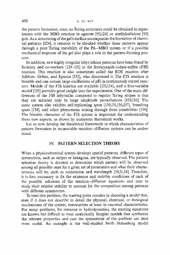
450 A . DE WIT
the pattern formation, since no Turing structures could be obtained in exper- iments with the MBO reaction in agarose [93,124] or methylcellulose [93] gels. As a structuring of the gel's surface accompanies the formation of chemi- cal patterns [124], it remains to be checked whether these patterns appear through a pure Turing instability of the PA-MBO system or if a possible mechanical response of the gel also plays a role in the pattern-forming pro- cess.
In addition, new highly irregular labyrinthine patterns have been found by Swinney and co-workers [129-1311 in the ferrocyanide-iodate-sulfite (FIS) reaction. This reaction is also sometimes called the EOE reaction after Edblom, Orban, and Epstein [132], who discovered it. The FIS reaction is bistable and can sustain large oscillations of pH in continuously stirred reac- tors. Models of the FIS kinetics are available [133,134], and a four-variable model [135] provides good insight into the experiments. One of the main dif- ferences of the FIS labyrinths compared to regular Turing stripes is that they are initiated only by large amplitude perturbations [129,130]. The same system also exhibits self-replicating spots [130,131,136,137], breathing spots [ 1381, and other phenomena arising through front instabilities [130]. The bistable character of the FIS system is important for understanding these new aspects, as shown by numerous theoretical works.
Let us now develop the theoretical framework in which characteristics of pattern formation in monostable reaction-diffusion systems can be under- stood.
1% PATTERN SELECTION THEORY
When a physicochemical system develops spatial patterns, different types of symmetries, such as stripes or hexagons, are typically observed. The pattern selection theory is devoted to determine which pattern will be observed among all possible ones for a given set of parameters and what their charac- teristics will be, such as orientation and wavelength [19,21,34]. Therefore, it is first necessary to fix the existence and stability conditions of each of the possible solutions of the reaction-diffusion equations and next to study their relative stability to account for the competition among patterns with different symmetries.
To treat this problem, the starting point consists in choosing a model that, even if it does not describe in detail the physical, chemical, or biological mechanisms of the system, summarizes at least its essential characteristics. For many problems, for instance in hydrodynamics, the starting equations are known but difficult to treat analytically Simpler models that synthetize the relevant properties and cast the symmetries of the problem are then most usefbl. An example is the well-studied Swift-Hohenberg model
SPATIAL PATTERNS AND SPATIOTEMPORAL DYNAMICS 451
[139]. In chemistry and biology, evolution equations are often simply not known, and the use of reaction-diffusion models can then be justified a for- tiori.
A linear stability analysis of the stationary steady states of these models determines at which values of the parameters different instabilities occur. In particular, it gives the critical value y c of the control parameter, above which the steady state becomes unstable because of a Turing instability and a new spatially organized solution appears. This Turing instability occurs when the growth rates of perturbations around the steady state are real and when one of them becomes positive for a wavenumber lkl = k, (see Section 11). Beyond this critical point, a certain number of spatial modes grow exponentially in time (Fig. 2). This linear exponential growth is saturated when the nonlinear terms in the evolution equations come into play The non- linear competitions between modes then select the preferred spatial planform and lead to a new spatial structure of finite amplitude, constructed with N - dominating modes. The description of the asymptotic behavior of the system beyond the instability threshold hence calls for a nonlinear approach of the problem.
A. Weakly Nonlinear Analysis
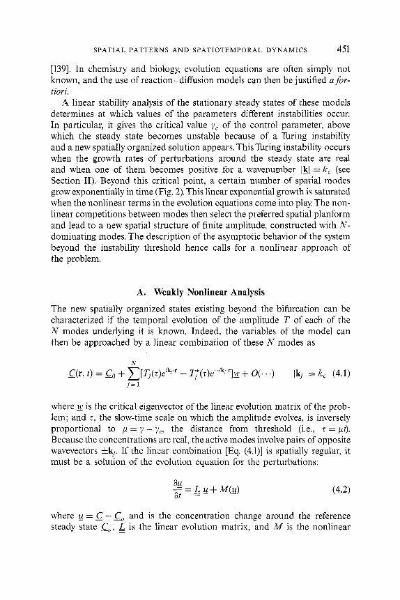
The new spatially organized states existing beyond the bihrcation can be characterized if the temporal evolution of the amplitude T of each of the N modes underlying it is known. Indeed, the variables of the model can then be approached by a linear combination of these N modes as
where g is the critical eigenvector of the linear evolution matrix of the prob- lem; and z, the slow-time scale on which the amplitude evolves, is inversely proportional to p = y - ye , the distance from threshold (i.e., z = pt). Because the concentrations are real, the active modes involve pairs of opposite wavevectors i k j . If the linear combination [Eq. (4.1)] is spatially regular, it must be a solution of the evolution equation for the perturbations:
where g = C - C, and is the concentration change around the reference steady state C,, L - is the linear evolution matrix, and A4 is the nonlinear

452 A . DE WIT
Figure 6. Bifurcation diagrams displaying the modulus R versus the bifurcation parameter p. The plain line and dashed line represent stable and unstable branches of solutions, respectively. (a) Supercritical case; (b) subcritical case; (c) saturated subcritical case, in which the stable non- linear branch of solutions appears with a finite amplitude at a secondary saddle-node bifurcation when p = pSN.
part in g. In the vicinity of the bifurcation, one seeks to determine g through an asymptotic expansion:
(4.3) 2 3 - U = E g l + E g2+E g3+ . . .
where the small expansion parameter E is related to the distance p from threshold as
(4.4) 2 p = y - y c = E y , + E y 2 + . . .
Solving the system of equations at each order in E allows us to obtain gl, g 2 , . . . , which define the structure of the nonlinear solution through the expansion [Eq. (4.3)]. If y1 # 0, the new solution reduces at lowest order to g - g,, with E - (y - yc)/yl , The solution g exists for both positive and negative F, and the bifurcation is said to be transcritical. If y1 = 0, we still have g - g,, but then E - Jm. The bifurcation occurs for y > ye if y 2 > 0 or y < y c if y2 < 0. The transition is then called supercritical or subcritical, respectively (Fig. 6). The dynamics of the system in the vicinity of the instability occur on different time scales than those of the reference steady state. Hence the partial differential operator in time is also developed in E as
(4.5) 2 a, = E a,, + E a,, + . . .
As the control parameter y usually comes into play in L,, we have -

SPATIAL PATTERNS AND SPATIOTEMPORAL DYNAMICS 453
where Lz_ , is the linear operator computed at B,. Substituting expressions (4.3)- (4.6) into (4.2) and isolating the different orders in E , the nonlinear initial problem gets down to solving successions of linear equations:
where i = 2, 3, . . . and LO = a, - L,. Eq. (4.7), at first-order, defines the criti- cal wave vector g,. Thisequation ichomogeneous in gl so that the amplitudes 7;. of the modes constructing this first-order solution remain unknown. The higher-order equations are nonhomogeneous and have a nontrivial solution only if their right-hand side is orthogonal to the kernel of L,;, the adjoint operator of Lz_ 0. This solvability condition, also called the Fredholm alterna- tive, determines at successive orders the different coefficients of the perturbation expansion (4.3) expliciting hence the new solution appearing beyond the instability, In particular, the Fredholm alternative makes explicit the amplitude T of the first-order solution by providing its temporal evolution equation, the so-called amplitude equation, which takes the general form:
(4.9) dT. A- - !-q + Gj({T;J) dt
where Gj({Ti}) are nonlinear polynomials in the active amplitudes. Details on the standard bihrcation techniques used to derive amplitude evolution equations can be found in [6,19,21,32,34].
The main advantage of the description in terms of amplitude equations is that close to the bifurcation point, the amplitude evolves on the slow-time scale of the critical modes that is inversely proportional to the distance from threshold. On this scale, the dynamics of the amplitude depends only on the type of instability Indeed, the terms appearing in the amplitude equations are functions only of the broken symmetries and not of the details of the system that appear only in the value of the coefficients of these equations [140]. Note that the amplitude equations were obtained by a perturbation expansion and are, therefore, valid only in the vicinity of the bifurcation point. Other descriptions of the system will be necessary farther away from threshold.
B. Degeneracies
The nonlinear analysis of the problem must take into account the degeneracies of the system. In small systems (the size of which is on the order of the critical wavelength), the spectrum of the linearized operator is discrete and at most

454 A . DE WIT
finitely degenerate [3,12,21,141]. Only a small number of modes are excited and the variables of the model can be constructed as a finite linear combination of these unstable modes. In that case, it can be shown that the reaction-diffusion system is correctly described by the reduced dynamics of the amplitude equations derived by standard bifurcation theory This is not true, however, for large systems, the boundaries of which are either at infinity or at such a far distance that they do not constrain the spectrum of spatial modes. The majority of experimental Turing patterns belong to the class of these large systems because several hundred of wavelengths are commonly obtained in the experiments.
The spectrum of unstable modes in large systems is then degenerated for two reasons. The first degeneracy is an orientational degeneracy In reac- tion-diffusion systems, the linear stability analysis shows that the growth rate of the unstable modes depends only on the modulus of the critical wave vectors. This means that the structures break the translational symmetry but not the rotational symmetry, All wave vectors lying on the sphere (or on the circle in 2D) of modulus Ik/ = k, are equally excited and must be included in the nonlinear treatment of the model. In other words, the number of linear combinations such as Eq. (4.1) is infinite. In practice, one chooses from among all possible combinations those that are linked to regular pavements of space, unless the focus is on more complex structures. This number N of modes used fixes the geometrical aspect of the pattern. For reaction-dif- fusion systems, the patterns considered in 2D for instance, are typically stripes ( N = l), squares ( N = 2), or hexagons ( N = 3). The linear combinations for N > 3 give rise to more complex multiperiodic structures [ 1421, such as those observed in experiments with parametric exci- tation [143,144] or in nonlinear optics [145]. These platforms have not been obtained in chemical systems and will thus not be considered here. A temporal evolution equation for the amplitude of the modes can be derived for each linear combination. To study the nonlinear competition between modes, one must first find solutions to the amplitude equations and then study their relative stability This procedure (discussed below) shows which structure will be observed based on the values of the parameters of the system and is thus the basis of the pattern selection theory [ 19,21,78,79,146].
The second degeneracy that we must deal with is continuous band quasi- degeneracy When the control parameter’s value is above criticality, there is a finite but continuous band of modes that become unstable in addition to the critical wave vectors (Fig. 2). In large systems, the number of such modes is so large that they form a quasi-continuous ensemble of modes of various lengths close to k,, spanning degenerate irregular spatial structures. This degeneracy can be treated by defining the amplitude as a

SPATIAL PATTERNS AND SPATIOTEMPORAL DYNAMICS 455
slowly variable function not only of time but also of space. In other words, we write
N
- C(r, t ) = Go + E [ ~ ( T , X)ezkj" + Tj* (z , X)e-'k~'r]w lkil = k, (4.10)
where the amplitude is now also a function of a slow space scale X. This space scale is proportional to to/cp - y,), where 5 , is the coherence length on the order of k;l. The amplitude equation, in that case, is a partial differential equation in space and time of the following form:
j = 1
9 = p q + Gj({Ti}) + (:02Tj (4.1 1)
where O2 is a spatial operator describing the modulation of the patterns on the long length scale. Amplitude Eq. (4.11) describes the nonlinear interactive behavior of the wave packets that account for the dynamics of all the modes included in the unstable band. Such envelope equations have become dynamic models on their own, because they reproduce numerous properties of nonequilibrium systems [ 19,211. They allow the study of defect dynamics, of localized structures in weakly nonlinear regimes, and of spatiotemporal chaotic dynamics.
The amplitude of a spatial pattern is a complex variable. Its modulus cor- responds to the intensity of the spatial modulation of the model's variables. Its phase is related to the breaking of translational symmetry. If the system is perturbed, variations of intensity relax on a slow characteristic time scale and are inversely proportional to the distance from the bifurcation tres- hold. The system remains neutral, however, in regard to a uniform phase change 7 j -+ Tjei@ that corresponds to a global translation of the pattern. The phase 0 thus evolves on an even slower time scale. Far from the bifur- cation point, the phase evolution on this time scale can then suffice to totally describe some properties of the system, such as typically long-wave instabil- ities. In that respect, phase equations have become a subject of research on their own [19].
at
C. Reaction-Diffusion Models vs Amplitude Equations
We have just seen that to tackle the pattern selection problem, two cornp- lementary points of view are available for theoreticians. The first one is to look at reaction-diffusion models. These models are the basis for an under- standing of the effect of changing parameters. The advantage of their numeri- cal integration is that the active modes are selected by the internal nonlinearities of the problem and not imposed a priori. Nevertheless,

456 A . DE WIT
from an analytical point of view, the thresholds of instability are often the only relevant quantities that can be obtained. The nonlinear regime must then be studied numerically.
The second tool available is that of amplitude equations that allow ana- lytical insight into the selection and possible transitions between different spatial planforms. Because the amplitude equations have a universal form and are a function only of the symmetries broken at the bifurcation point, the advantage of studying them is that all bifurcation scenarios predicted on their basis are applicable to any physicochemical system that presents the related breaking of symmetries. The disadvantages are that amplitude equations are valid only in the vicinity of the bifurcation point and that they depend on the modes considered. They are hence of no help if one does not know which modes are involved a priori.
V. TURING PATTERNS
The theoretical approach devoted to understand which types of patterns can be observed in reaction-diffusion systems and what their succession will be when a control parameter is varied is now outlined for 2D and 3D systems.
A. Reaction-Diffusion Models
To study pattern formation in chemical systems owing to the coupling of chemical reactions and diffusion processes, it is natural to turn to reac- tion-diffusion models [12,147]. The best model is, of course, the one that is the closest to the experimental system, as the ultimate goal of any theory is quantitative predictions. Unfortunately, chemical kinetics are often com- plicated; thus it is useful to study typical bihrcation scenarios via simpler models that are more easily mathematically handled.
Several works on Turing patterns have focused on quantitative comparison with experimental results. The Lengyel-Epstein model is the most realistic model available for quantitative comparisons with the CDIMA reaction [50,54,57]. This model provides structures with wavelengths that are in good agreement with those observed experimentally [58,122,123] and has been used to obtain conditions on possible three-dimensionality of the pat- terns in parameter space [58]. Jensen and co-workers thoroughly investigated the 1D and 2D pattern selection problem of the Lengyel-Epstein model [88,100,120,121,148,149]. They show that, in one-dimension, it exhibits a strong subcriticality of stripes and bistability between the stripes and a Hopf state. In the subcritical regime, a study of the wavenumber selection and propagation speed was performed in the case of a moving front between the stripes and the homogeneous steady state [120]. Pinning effects resulting in a van-

SPATIAL PATTERNS AND SPATIOTEMPORAL DYNAMICS 457
ishing front velocity because of interaction of the front with the underlying Turing pattern were evidenced [ 100,120,121].
In two dimensions, both stripes and hexagons appear subcritically. As a consequence, many localized structures exist in the domain of parameters for which bistability between two different states occur. In particular, stable spatial coexistence of stripes and hexagons [88], patches of hexagons embed- ded into the homogeneous steady state [88,120], and growing mechanisms of hexagons into a homogeneous background [120] were obtained in the Lengyel-Epstein model and enlighten the recent experimental observations of some of these phenomena [80]. Localized Turing-Hopf structures were also observed in the Turing-Hopf bistability regime of the Lengyel- Epstein [100,120,149].
Another model that has been extensively studied in the framework of pat- tern formation in chemical systems is the two-variable Schnackenberg model [150]. Dufiet and Boissonade showed that this model reproduces 2D patterns seen in the experiments and clarifies long-wave instabilities, such as zigzag or Eckhaus instabilities of patterns [86,87]. Quantitative com- parison between analytical predictions and numerical simulations made with the Schnackenberg model have greatly helped test pattern selection theories [48,86,87,151].
Recently, a good insight into such comparisons was provided by the ad hoc construction of reaction-diffusion models in which the coefficients in front of the variables in the model are simply related to those of the amplitude equations [48,104]. Note that prototype models for pattern formation, such as the Swift-Hohenberg model [139], have also been studied in relation to chemical problems [90,99,152].
In this chapter, we mainly focus on the Brusselator model [3,153]. This two- variable model can exhibit both aTuring and a Hopf instability. Its advantage is that the base state, the thresholds of both instabilities, and the coefficients of the related amplitude equations for pattern formation or temporal oscilla- tions are straightforwardly obtained analytically [9,97,154,155]. Moreover the Brusselator model has been the subject of many studies, so we have a good knowledge of the possible spatiotemporal dynamics it can exhibit [3,75,79,119]. It is, therefore, the model we will focus on in this review, because it has been used to analyze most of the topics discussed here. The reac- tion-diffusion equations of the irreversible Brusselator are as follows:
a,x = A - ( B + 1)X + X 2 Y + D, v2x a,Y = BX - x2 Y + D, v2 Y (5.1)
The concentration of species B is usually chosen as the bifurcation par- ameter. The homogeneous steady state (&, Y,) = ( A , B/A) of system Eqs.

458 A . DE WIT
(5.1) undergoes a Turing instability when B > BT = (1 + A , / m ) 2 . A stationary spatial pattern then emerges, characterized by an intrinsic critical wave vector k: = A/- . The steady state may also go through a Hopf instability if B > BY = 1 + A 2 , evolving then into an homogeneous limit cycle characterized by a critical frequency oc = A . The thresholds of these two instabilities coincide at a codimension-two Turing-Hopf point, defined as the point at which B," = B,'. This condition is achieved when the ratio of the diffusion coefficients g = D,/D, reaches its critical value
Note that these models do not exhibit some of the hndamental charac- teristics of the experimental reaction-diffusion systems, such as bistability, excitability, and formation of traveling waves owing to a Hopf bihrcation with a nonzero wavenumber. This latter instability occurs only in three-vari- able models. Because bistability is an important characteristic of the FIS reac- tion, some studies devoted to understanding spatial patterns formed in that system have used the bistable FitzHugh-Nagumo model [ 156,1571, the Gaspar-Showalter model of the FIS reaction [134,135] and the Gray and Scott model [158].
r7, = [ (d i -Tz - 1)/AI2.
B. Two-Dimensional Pattern Selection
In this section, we will briefly illustrate the nonlinear analysis techniques sket- ched in Section IV to study the 2D pattern selection problem in reaction- diffusion systems in the weakly nonlinear regime. To do so, we will first neglect any possible spatial variation of the mode's amplitude and obtain standard bihrcation diagrams that are valid in the vicinity of the bihrcation point. We will then discuss specificities of chemical systems, such as re-entrance of hexagons and localized structures in subcritical regimes before comment- ing on effects induced by spatial modulations of the amplitudes.
1. Standard Bifurcation Diagram
Let us successively consider amplitude equations for the regular 2D spatial structures constructed with one (stripes), two (squares), or three (hexagons) pairs of wave vectors.
A perfect periodic structure in only one direction of space, such as stripes, is built on one pair ( N = 1) of wave vectors; and in that case, the concen- tration field [Eq. (4.1)] can be constructed as
- C(r, t ) = Go + [T(z)eik"' + T*(z)e-ik1'']41r: (kll = k, (5.2)

SPATIAL PATTERNS AND SPATIOTEMPORAL DYNAMICS 459
At the lowest order, the amplitude equation for T, derived using techniques discussed in Section IYA, reads
d T -=pT -glT12T dt (5.3)
The amplitude T is imaginary, and if we separate its modulus and phase, writing T = Rei8, we get
d R - = pR - gR3 dt _ - - 0 dB dt
The phase can take any constant value, a signature of translation invar- iance. The phase may thus be set to zero by a suitable choice of coordinates. The modulus equation [Eq. (5.4)] has two stationary solutions: either Rs = 0, characterizing the homogeneous steady state, or R, = m, corre- sponding to stripes. Two subcases can be distinguished: if g > 0, the bihr- cation is supercritical, and the new solution exists for ,u > 0; whereas if g < 0, the new solution arises for p i 0, and the bihrcation is subcritical. In both cases, we have a pitchfork bifurcation [19,21].
To investigate the stability of these solutions, a standard linear stability analysis of each of them must be performed. The difficulty in the analysis arises from the fact that for each state one must discuss the stability with respect to all possible types of perturbations: phase, modulus, orientation of the wavevector, and resonant perturbations to other structures with differ- ent symmetries. Let us first consider perturbations of the modulus (the other perturbations will be considered later). Writing R = R, + 6R, and inserting it into Eq. (5.4), we see that the trivial state R, = 0 looses stability when p > 0, whereas the stripes are stable for p > 0 if g > 0. If g < 0, the stripes that arise subcritically are unstable for ,u < 0, as the instability is not saturated by nonlinear terms. The bifurcation calculation must then be carried out to higher orders, where we get the following amplitude equation:
dT -=pT -glT12T-g’jT14T dt
If g’ is positive, the bihrcation saturates, leading to stripes that appear sub- critically at the point ps, = -g2/4g‘, where a secondary saddle-node bifur- cation occurs [Fig. 6(c)]. The stability of the various branches are then calculated in a standard fashion. For psN < p < 0, there is bistability between the stripes and the trivial homogeneous state, with the possibility of observing

460 A. D E WIT
localized structures (see Section V.B.3). If g' is negative, the bifurcation is not yet saturated, and we must proceed at still higher orders.
Let us now consider 2D structures built on more than one pair of wave vectors that are regular pavements, i.e., pavements for which the N pairs of modes make z / N angles between them. When N = 2, this corresponds to squares for which the concentration field becomes
where c.c stands for complex conjugate. The corresponding amplitude equations for squares are
with j , 1 = 1 ,2 and 8 = 7c/2. We see that a nonlinear coupling term between the two sets of modes must now be taken into account. Let us consider here the cases in which the instability is saturated at this order, i.e., g > 0, g N D > 0. Writing ~j = Rje"], we get
(5.9)
(5.10)
In the case of stripes, the constant factor phases correspond to a simple translation of the pattern. The solutions to the evolution equation for the mod- ulus Rj are the trivial homogeneous steady state (R1 = R2 = 0) and stripes corresponding to R1 # 0, R2 = 0 (stripes perpendicular to k l ) or R1 = 0, R2 # 0 (stripes perpendicular to k z ) . The squares correspond to the case R1 = R2 = RR, with
(5.11)
A linear stability analysis of these supercritical branches shows that squares and stripes are mutually exclusive, i.e., stripes are the stable pattern if g < g N D , and squares are stable if g > g N D . Note that, if the system is even slightly anisotropic, 0 might be different from n/2, and the squares then become rhombs. As the coefficient g N D takes values that vary with 8, the stability domain of these rhombs may differ with that of the squares; but nevertheless, they remain unstable in regard to stripes as long as g < gND(B).When 8 = n/3, the Eq. (5.8) for rhombs is no longer valid, because in such a case, the vector kl + k2 falls on the circle of critical wave vectors and

SPATIAL PATTERNS AND SPATIOTEMPORAL DYNAMICS 461
(a) (b)
Figure 7. The resonance condition on the circle of radius k,. (a) Nonresonant combination of two wave vectors kl and k2: Their sum is wave vector k with Ikl # k,. (b) Resonant combination of two wave vectors that make an angle of 2z/3 between them and, therefore, excite a third critical wave vector.
is excited as well (Fig. 7). Its dynamics must then be taken into account. The resulting pattern is a regular structure corresponding to hexagons and con- structed with three pairs of wavenumbers ( N = 3) such that kl + k2 + k3 = 0. The amplitude equations for these three modes are
(5.12)
The amplitude for the two other modes are obtained by cyclic permuta- tions of the indices. These amplitude equations and in particular the quadratic term present in Eq. (5.12) can be obtained only in systems for which the T -+ -T symmetry is broken. This is, for instance, the case in non- Boussinesq Rayleigh-Benard convection [ 191 or typically in chemical sys- tems. As in the case of rhombs, the coefficients g and h of the coupling term are functions of the angles between the three wave vectors. For the sake of simplicity, let us assume that g and h are positive and that the hex- agonal pavement is regular, i.e., the angle between modes is strictly equal to n/3. The evolution equation for the sum of the phases 0 = 81 + 6, + 83 reads
sin 0. (5.13) R:R: + R:Ri + R, 2R21 dO
dt R1 R2R3
Contrary to the cases of stripes and rhombs, the phases of hexagons are not free to translate independently Two phases are free, because we have two degrees of translation freedom on a plane and the third phase is fixed by the dynamics of the system. The evolution Eq. (5.13) has two stationary sol-
462 A . DE WIT
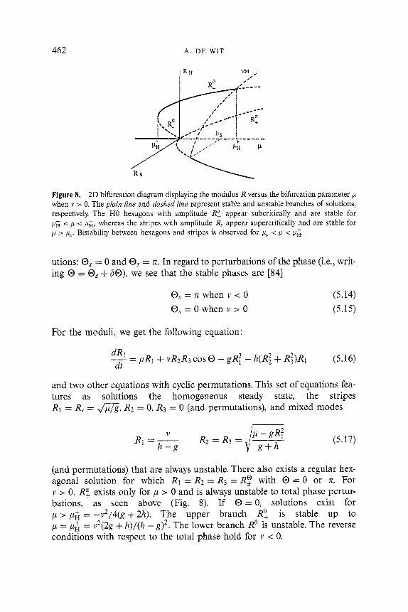
Figure 8. 2D bifurcation diagram displaying the modulus R versus the bihrcation parameter ,u when v > 0. The plain line and dashed line represent stable and unstable branches of solutions, respectively. The HO hexagons with amplitude R: appear subcritically and are stable for p~ < ,u < p&, whereas the stripes with amplitude R, appear supercritically and are stable for ,u z p,. Bistability between hexagons and stripes is observed for p, < p < ,u&
utions: 0, = 0 and 0, = n. In regard to perturbations of the phase (i.e., writ- ing 0 = @, + SO), we see that the stable phases are [84]
0, = n when v < 0 0, = 0 when v > 0
(5.14) (5.15)
For the moduli, we get the following equation:
(5.16)
and two other equations with cyclic permutations. This set of equations fea- tures as solutions the homogeneous steady state, the stripes R1 = R, = m, R2 = 0, R3 = 0 (and permutations), and mixed modes
dR1 dt - = pR1 + v R ~ R ~ cos 0 - gR: - h(R2 + Ri)R1
(5.17)
(and permutations) that are always unstable. There also exists a regular hex- agonal solution for which Rl = R2 = R3 = RZ with 0 = 0 or 71. For v > 0, RT exists only for ,u > 0 and is always unstable to total phase pertur- bations, as seen above (Fig. 8). If 0 = 0, solutions exist for p > p g = -v2/4(g+2h). The upper branch R! is stable up to ,u = ,u& = v2(2g + h) / (h - g)2. The lower branch Ro is unstable. The reverse conditions with respect to the total phase hold for v < 0.

SPATIAL PATTERNS AND SPATIOTEMPORAL DYNAMICS 463
r l x i ?h 1 fc j
Figure 9. Stationary 2D Turing structures. The concentrations vary between their absolute mini- mum (black) and maximum (white) values. (a) HX hexagons for which the maxima are on an hexagonal honeycomb lattice, (b) stripes, (c) HO hexagons for which the maxima are on a tri- angular lattice.
Depending on the sign of the quadratic coupling v, the first hexagonal phases to appear subcritically are thus either HO hexagons ( v > 0 and 0 = 0), for which the maxima of concentrations are organized as a triangular lattice [Fig. 9(c)], or Hn hexagons (v < 0 and 0 = n), for which the maxima of concentrations span a honeycomb lattice [Fig. 9(a)]. In chemical systems, one type of hexagon is commonly observed in experiments, whereas the other type of hexagon appears only transiently (Fig. 1). Two types of hexagons have also been observed in Faraday instability [ 1591, in oscillated granular layers [160,161], in nonlinear optics [ 162-1641, and in hydrodynamics [19].
To complete the bifurcation diagram, it is also necessary to study the stab- ility of stripes in regard to perturbations favoring hexagons. Writing R1 = R, + 6R1, R2 = 6R2, R3 = 6R3 and inserting this into Eq. (5.16), we see that stripes are unstable with respect to the formation of hexagons, if
To summarize the pattern selection in 2D, a supercritical branch of stripes is stable if g < g N D , whereas a supercritical branch of rhombs is obtained when the reverse is true. In all reaction-diffusion models studied to date, one usually has g < gND, and stripes are observed. In addition, a branch of hexagons can appear subcritically with a finite amplitude (Fig. 8). Depending on the sign of the quadratic term v, these hexagons are HO- or Hn hexagons and become unstable when P > P,. The stripes are unstable for p < pp Stripes and hexagons thus coexist for p s < p < yH. This bifix- cation scenario corresponds to the standard hexagon-stripe competition, widely described in the literature [19] and observed in hydrodynamics [73,77], nonlinear optics [162,164], and gas discharges [ 165,1661 among others. This standard roll-hexagon competition is recovered in the experimental Turing patterns [48,91] and in reaction-diffusion models [84,86,120]. In
P < P, = v2g/(h - gI2.

464 A . DE WIT
that respect, chemical systems join the group of pattern-forming systems that present a generic behavior. Modification of this scenario in the vicinity of the primary bifurcation point p = 0 arises if g and/or h are not positive. If g < 0 but g + h > 0, stripes appear subcritically, as seen in the Lengyel-Epstein model [ 1201, whereas hexagons are still well described by the third-order amplitude Eq. (5.12). If both g and h are negative, the ampli- tude equations for the stripes and hexagons are both saturated only at higher orders, and the pattern selection is consequently different.
Let us now focus on the peculiarities of chemical systems that bring some complexity into this standard 2D picture of pattern selection.
2. Re-entrant Hexagons
We have seen that the sign of the quadratic term v controls the type of hexa- gons (HO or HTC) observed. Chemical systems are characterized by the fact that the sign of v may change within a given experiment following an increase of the control parameter. This arises because the control parameter often multiplies one variable in the kinetic terms of the reaction-diffusion equations. In the Brusselator model for instance, the control parameter B appears in terms proportional to BX in the evolution equations for the two variables X and Y. This results in the fact that, sufficiently far away from the bifurcation point, the coefficients of the amplitude equations are renormalized by the distance p from the bifurcation threshold, i.e., we typically have < = 2 + p t1 , In the Brusselator model, for example, the quad- ratic term v is equal to [84]
(5.18)
where A is a parameter of the model [Eqs. (5,1)], This affects the stability of hexagons and the stability of stripes in regard to hexagons. If V is positive, then the overall quadratic term v remains positive when B is increased beyond B,, and HO hexagons are stable toward stripes up to p$ = v2(2g + h)/(h - g)2. If on the contrary, V is negative, which means that Hn hexagons are the first stable structure to appear subcritically, then an increase of B can change the sign of v and lead to the switch from one type of hexagon to the other. We thus have the succession Hn, HxlS, S, WHO, HO (where AIB indi- cates bistability of structures A and B). This sequence was first observed numerically in reaction-diffusion models [84,86] (Fig. 10) and then con- firmed experimentally in the CIMA reaction [66]. A complete analysis of the effect of renormalizations carried out for the Schnackenberg model [150] showed that, depending on the parameter values, other scenarios such as S , SIHO, HO; HO, HOIS, S, SIHO, HO; HO, HOIS, HO; and HO are

SPATIAL PATTERNS AND SPATIOTEMPORAL DYNAMICS 465
4 - i 10 15 20 25 B
Figure 10. Numerical bifurcation diagram for the variable X of the Brusselator model as a function of parameter B. Here the amplitude is defined as X,,, - X,. The parameters are A = 4.5, D, = 7, and D, = 56. Near the bifurcation threshold (B, =6.71), we recover the standard hexagon-stripe competition with an hysterisis loop, and hexagons with the reverse total phase become stable for higher values of B.
also possible and are sometimes seen in experiments [48]. Note that a renor- malization of the quadratic term v can also result from a coupling with a bistable regime (see Section VILA). Re-entrance of various planforms can also be the result of the presence of higher-order terms in the amplitude equation because in that case the standard bifurcation scenario is also modi- fied [99].
3. Localized Structures in Subcritical Regimes
The standard bifurcation theory predicts that the hexagons should appear subcritically, leading to a bistability regime between the hexagons and the homogeneous stable steady state. In addition, stripes may appear subcritically, as seen before. This situation is encountered in the Lengyel-Epstein model, which features a strong subcritical regime of stripes in 1D and of both hexa- gons and stripes in 2D [@I. In this subcritical domain, different steady states coexist; and the system usually evolves toward one or the other solution, depending on the initial condition. A common way to know which state is dominant is to look at the propagation of wavefronts connecting the two states, because in this case the prefered state invades the other one.
In lD, Jensen and co-workers [120] studied such propagating fronts on the Lengyel-Epstein model in the subcritical regime. They observed that the wavenumber selected when a stable striped structure invades the homo- geneous steady state is different from that obtained from spontaneous growth of the pattern out of noise added on the homogeneous steady state [12,167]. Moreover, there exists a band of values of the control parameter

466 A. DE WIT
for which the velocity of the front vanishes, giving rise to a stable stationary front between the homogeneous steady state and the Turing structure, The stability of such a front is related to the interaction of the front with the period- icity of the spatial organization [79,168-1701, a so-called nonadiabatic effect common in solid state physics. This effect, which is not contained in the amplitude equation formalism, can occur for fronts between two states, one of which is periodic in space [168]. It appears, for instance, in the growth of crystals, in which the interaction between the interface and the periodic structure gives rise to a periodic potential. If the difference in free energy between the two phases is smaller than the energy required to move the front by one wavelength, the front remains pinned. The Lengyel-Epstein model is a nonpotential model; thus one cannot define a function to mini- mize. The picture of an interaction between the front and theTuring structure, however, remains qualitatively correct and gives rise to an intrinsic pinning of the front for a large set of values of the control parameter. Calculation of the front velocity via the usual techniques [171-1731 shows a change in behavior at the crossover between the subcritical and the supercritical regimes. In par- ticular, in the subcritical domain, the front no longer moves uniformly but jumps one wavelength at a time, the interval between two successive jumps increases as the pinning band is approached. Such interactions are also the result of the interaction between the front and the Turing pattern. The interaction between two fronts can lead to the formation of stable pulses
In 2D, the Lengyel-Epstein model exhibits subcriticality of both hexagons and stripes. There thus exists a range of parameters for which tristability among the hexagons, stripes, and homogeneous steady state occurs. As in lD, localized structures of one of these states into another stable one can occur; and indeed, stable patches of hexagons inside a homogeneous back- ground are obtained (Fig. 11). Note that such localized hexagons have been recently observed experimentally in the CDIMA reaction and that this observation could point toward a subcritical regime [80,91]. Such loca- lized hexagons can also appear in the strong resonant forcing of oscillators [ 179,180] or because of localized heating in thermocapillary convection [ 1811. Another possible localized structure consists of stripes coexisting with hexagons [88,120]. In 2D, the growth of fronts between different types of structures [170,182] is, nevertheless, not as simple as in lD, because pinning occurs only when the front is perpendicular to the wave vectors of the pattern [120]. Hence the growth of subcritical localized hexagons out- side the pinning zone is qualitatively different from that of supercritical hexa- gons inside an unstable background. In the former case, hexagons grow by adding new points in the directions in which the pinning is the weakest, as observed in the subcritical region of the Lengyel-Epstein model. In
[ 174- 1781.

SPATIAL PATTERNS AND SPATIOTEMPORAL DYNAMICS 4 67
Figure 11. integration of a generalized Swift-Hohenberg model. From Ref. [loll.
Subcritical hexagons localized in a homogeneous background obtained by numerical
the growth of supercritical hexagons, stripes form along the sides of the hexa- gons and successively break up into dots, as seen in experiments with the PA- MBO system [93], in convection cells [170], and in the Brusselator [120] model, for instance.
4. Boundaries
Let us now examine how the perfect stripes and hexagons can be affected by boundaries. In reaction-diffusion systems, boundaries have an important effect on the characteristics of patterns, such as selection and orientation of patterns and the relaxation time necessary to obtain a stationary spatial structure or to relax a defect. These effects are particularly important in small systems in which only a few wavelengths develop [3,21,85,183-1881,
Figure 12 compares hexagons obtained at a same time for the same values of parameters and starting from the same random initial condition in a small system with periodic, no flux, or fixed boundary conditions. The peri- odic boundary conditions lead to regular planforms, and the periodicity for-

468 A . DE WIT
Figure 12. Hexagons obtained by numerical integration of a 2D Brusselator model with A = 4.5, D, = 7, D, = 56, and B = 7, starting from the same random noise initial condition in a system of size 64 x 64. (a) Periodic boundary conditions; (b) no flux boundary conditions; (c) conditions fixing X = X, = A and Y = Y, = B / A at the boundaries.
ces the pattern’s alignment. Nevertheless, if the length of the system is not exactly an integer multiple of the wavelength, the periodic boundary con- ditions give rise to a distortion of the hexagonal planform, as shown in Figure 12(a>, in which the angle between the wave vectors is not exactly 71/3 and the hexagons look rather like rhombs. Periodic boundary conditions partially lift the orientational degeneracy of the initial condition, because the wave vectors can align only along the directions that allow the periodicity to be achieved. Symmetry group arguments [I891 have shown that in a square domain with periodic boundary conditions, rhombic patterns and even more complex structures have the potential of being stable [141]. Rhombs can also have other origins: Temporal forcing of hexagons can select rhombic arrays in some cases [190]. Nonequilateral patterns based on two or three wave vectors of different lengths also occur when rotational invariance is broken [191]. It is, therefore, necessary to be cautious when determining whether rhomblike structures observed experimentally in small aspect ratio systems result from a distortion of hexagons because of the boundaries or from a genuine stable solution of the pattern selection problem. A Fourier transform of the pattern can be of some help in that regard, as pure rhombs are characterized by two Fourier modes of same amplitude, whereas deformed hexagons correspond to three peaks of different ampli- tudes.
No flux boundary conditions also lead to the rapid development of the structures but often result in a distortion of the pattern close to the boundaries [Fig. 12(b)]. Dufiet and Boissonade showed for instance, that striped patterns develop preferentially orthogonally to the walls when no flux boundary con- ditions are applied [87]. In the middle of the system, the intrinsic wavelength is not constrained, and hexagons develop according to the directions privi- leged by the initial condition. The fixed boundary conditions, on the

SPATIAL PATTERNS AND SPATIOTEMPORAL DYNAMICS 469
other hand, strongly constrain the structure and easily lead to the formation of defects [Fig. 12(c)]. Note that several studies have used mesoscopic lattice-gas cellular automaton models to examine the effects of fluctuations and small system size on Turing structures [192-1961.
5. Long-Wavelength Instabilities and Phase Equations
In systems large enough that several dozens of wavelengths develop, boundary conditions usually play a role limited to a little layer close to the boundaries. In such a case, starting from random initial conditions, the orientational degeneracy leads to the formation of domains with different orientations. The compatibility between these domains is ensured by the presence of defects. The defects that evolve on a long time scale are typically dislocations, disclinations, or grain boundaries in stripe structures or penta-hepta defects in hexagons. Numerous works characterized such defects in detail [9,19,21,34,197-2001 and clarified in particular the interactions among them [201,202]. A particular type of defect [170,182,203] is the boundary between two different types of 2D spatial structures. Defects also play a role in the transition between patterns of different symmetries [204]. Some studies have indeed shown that the unstable planforms are present in the heart of the stable patterns defects [76,202].
Beyond the influence of boundaries and defects, patterns can also be deformed because of modulational instabilities owing to a spatial modulation of the amplitude of their underlying modes. For example, Figure 13 shows zigzag stripes obtained in the Brusselator model. These stripes coexist with straight rolls for the same parameter values. One or the other structure is obtained, depending on the initial condition. In this context, Dufiet and Boissonade studied the generical instabilities of the stripes in great detail on the Schnackenberg model 1861. The zigzags are stable until the angle of the deformation reaches n/3, when they become unstable toward hexagons [85]. The zigzag branch exists because of the competition between wave vectors belonging to the same band of unstable modes. This effect can be described only if we take a spatial variation of the amplitude into account. Straight stripes with their wave vector aligned along x with Ik] = k, can be described as
(5.19)
On the other hand, zigzags imply a transverse modulation along direction y . They can thus be described as a first approximation as
(5.20)

470 A. DE WIT
Figure 13. Figure 10, and B = 8.
Zigzag stripes observed in the Brusselator model for the parameter values given
This modulation leads to a change in the local value of the wave vector or equivalently of the stripes phase. The amplitude equation taking this spatial effect into account is the Newell- Whitehead- Segel (NWS) equation [205,206]
aT - = p T - I T I 2 T + ar
(5.21)
where X and JJ are the length scales on which the spatial modulation of the amplitude occurs. This equation can be derived [21] by the standard pertur- bation expansion techniques if the slow time and space scales are developed as z = E 2 t , X = EX, Y = ~ f y . The NWS equation features as solution the straight stripes with wavevector Q:
TQ = 4- eiQx + C.C. Q2 < p (5.22)

SPATIAL PATTERNS AND SPATIOTEMPORAL DYNAMICS 471
where Q belongs to the band of unstable wave vectors, i.e., is proportional to k - k,. To study the stability of these straight stripes in regard to modulus and phase perturbations, let us take
(5.23)
In the absence of spatial derivatives in the amplitude equations, we recover the stability analysis described previously in the construction of the bifurcation diagrams. If this expression is now inserted into the NWS equation we get at the lowest order the evolution equation for the phase O(z, X, y) :
&d = DxV$O + DyV$ (5.24)
with
(5.25)
When the phase diffusion coefficients D x and Dy become positive, the longitudinal and transverse perturbations relax through a diffusive process, and the straight rolls are stable. On the other hand, the stripes are unstable toward long-wavelength instabilities if these diffusion coefficients are negative. When Q < 0, D y becomes negative, and the stripes are transversally modu- lated through a zigzag instability [207-2091; but if Q2 < p < 3Q2, DX becomes negative, and the bands are longitudinally modulated (Eckhaus instability) [210,211]. Higher-order terms in Eq. (5.24) could saturate this insta- bility, which explains why stable zigzags can be obtained in experiments [48,66,91,124] and numerical simulations [86].
Analogous modulational instabilities occur in hexagonal planforms. For example, an Eckhaus instability of one of the three modes forming a hexag- onal planform is shown in Figure 14. Phase equations for hexagonal planforms have recently been derived [ 182,212-2141, and their long-wavelength instabil- ities have been analyzed [212-2141.
Here it is important to note that the spatial derivatives appearing in the NWS Eq. (5.21) for stripes take this form only because we assumed at the beginning that the stripes were aligned along x. This apriori choice supposes that one direction is privileged. Recently, a debate appeared in the literature arguing that amplitude equations should satisfy rotational invariance [34,90,215-2191. In that case, the spatial derivatives present in the amplitude equations are different from those in the NWS. The main consequence of the new nonlinear gradient terms [220,221] that appear in the amplitude equations satisfying such rotational invariance is that they affect the stability of the different planforms and, in particular, allow the stabilization of rhombs

472 A . DE WIT
Figure 14. Eckhaus instability of one of the three wave vectors that underly an HO hexagonal planform. The succession in time must be read from top to bottom and left to right. The starting HO hexagons are obtained in the Brusselator model for A = 2, D, = 4, D j = 20, and B = 4.5.When B is increased to 5.5, the original wavelength is too large and an Eckhaus instability takes place.
[89,90,215,221], such as those observed in the CIMA reaction, which are other- wise unstable in the standard bifurcation theory.
C. Three-Dimensional Pattern Selection
One of the main characteristics of the experimental Turing structures is that they are generally three-dimensional objects [47,48,64,69,70,72,98] as soon as the wavelength of the pattern is smaller than any side of the region of the gel in which the symmetry-breaking instability takes place. Hence the pattern selection problem must take into account the possible new structures that arise in 3D.
1. Bifurcation Diagrams
As in 2D, the 3D pattern selection approach starts by writing the concen- tration in the system as a linear combination of N modes, such as Eq. (4.1). Each 3D structure is also characterized by the number N of modes that underlie its construction. The general temporal evolution equations for the amplitudes Ti with i = 1, . . . , N become in absence of spatial

SPATIAL PATTERNS AND SPATIOTEMPORAL DYNAMICS 473
modulations [79,117,222] :
The coefficients gND(i j ) and p(ijkl) are functions of the angles between the wave vectors considered. Among the solutions to these amplitude equations, we recover the N = 1,2, 3 solutions already studied in 2D. If N = 1, the stripes become 3D parallel isoconcentration planes, also called lamellae. The 3D extension of the rhombs with N = 2 are prisms, with a rhombic base; whereas the hexagons (N = 3) correspond to hexagonally packed cylin- ders (HPC). The relative stability of these patterns extend into 3D the con- clusions drawn in 2 4 i.e., in the simplest case, lamellae appear supercritically, the rhombic prisms are unstable with respect to the lamellae if g D < g N D and HPC arise through a subcritical bifurcation. The total phase of the HPC's hexagonal basis relaxes either to 0 or ?I, giving rise to two possible solutions: the HPCO or the HPCn.
The interest of the 3D pattern selection problem lies in the possibility of getting new structures that have no 2D equivalent. If N = 4, for instance, the basic wave vectors can form noncoplanar quadrilaterals (kl + k2 + k3 + k4 = 0) in Fourier space, a combination corresponding to a face-centered cubic (FCC) structure in real space [223]. Again, the con- dition g D < g N D ensures that the FCC structure is unstable. If N = 6, a maxi- mum number of resonances [224] is obtained if the six wave vectors are aligned along the edges of a regular octahedron (Fig. 15) which corresponds
Figure 15. 3D body-centered cubic symmetry In Fourier space, the six pairs ofwave vectors are parallel to the edges of a regular octahedron. Each pair is involved into two nonplanar resonant triads. From Ref. [151].

414 A. DE WIT
in real space to a body-centered cubic (bcc) structure. In this case, each wave vector belongs to two equilateral triangles, and the following three indepen- dent resonance conditions must be satisfied [151]:
(5.27)
Recalling that the amplitudes T j = RjeieJ, the resonance conditions on the wave vectors in Fourier space come down to conditions on the phases 0,. It can be shown that three independant phases 0 1 = 81 +02 + 03, 0 2 = 81 + 8 4 + 85, and O3 = 82 - 8 4 + O6 must be known to completely characterize the BCC pattern. A stability analysis of the BCC pattern indi- cates that only two possibilities exist:
(5.28) (5.29)
(a)
Figure 16. Continued opposite.

SPATIAL PATTERNS AND SPATIOTEMPORAL DYNAMICS 475
(bl
Figure 16. 3D BCCz Turing pattern obtained by numerical integration of the Brusselator model in a cube with sides equal to 40 and periodic boundary conditions along the three axes. The parameters are A = 4.5. D, = 2, Dj = 16. and B = 6.9. Isoconcentration surfaces are looked at perpendicularly to one face of the cube. (a) Spheres of lower isoconcentrations ( X = 2.737) organized with the BCC symmetry; (b) higher isoconcentrations (X = 5.153) filling in the interspace between the lower isoconcentrations.
The corresponding structures are thus called BCCO and BCCn. In real space, BCCO has its maxima of concentrations organized as a body-centered cubic lattice, whereas the minima fill in the interspace between the maxima as fila- mental structures with cubic symmetry The reverse situation is obtained in the BCCn case (Fig. 16). The relative stability analysis of the BCC structure with the other 3D patterns shows that the BCC pattern arises subcritically and becomes unstable toward the HPC at higher values of the control parameter. A succession of BCC-HPC-lamellae with regions of bistability is, therefore, predicted analytically; the total phase of the BCC depends on the sign of the quadratic term v 175,117,222,2251. This bifurcation scenario was confirmed

476 A. DE WIT
7 , , , , , , , , , , , _ , / , , , , , , , , , , , , ,
c
4
3
2
i 1 ' I I , I , ,
6.8 7 7.2 7.4 7.6 7.8 0 B
Figure 17. 3D numerical bifurcation diagram obtained with the Brusselator model for the set of parameters given in Figure 16 and varying the control parameter B. The amplitude here is defined as x m a x - Xmm
by numerical integration of the Brusselator model (Fig. 17) [117] and bears analogies with those occuring in equilibrium systems [226]. It was suggested that other 3D patterns, for instance a double-diamond structure in which the maxima and minima form two interlocked diamond lattices, could be stable as well [79,227]. In fact, a classification of the primary solution branches of different lattices with periodic boundary conditions was performed in 3D by Dionne and co-workers [228,229]. Callahan and Knobloch checked the stability conditions of several of these 3D patterns (including FCC and double-diamond structures) on three cubic lattices [227,230,231]. In particu- lar, they specified parameter regions in the Brusselator model [227,231] and the Lengyel-Epstein model [231] for which rolls, FCC, or the double-diamond should be stable with respect to perturbations on these lat- tices. Unfortunately, these values are outside those already scanned in 3D numerical simulations [117,222]. It remains to be checked how these con- clusions generalize to arbitrary boundary conditions and spatially extended systems. The problem is even more complicated as evidence exists that out- side the weakly nonlinear regime, the traditional pattern selection compe- tition is drastically changed when higher harmonics come into play [232,233]. Such effects should be kept in mind when experimental data are analyzed.

SPATIAL PATTERNS AND SPATIOTEMPORAL DYNAMICS 477
2. Minimal Surfaces
The experimentally observed 3D Turing patterns could be compatible with the BCC, HPC, or lamellae symmetries [63,64,72] predicted by the theoretical works. Nevertheless, a clear interpretation of the experiments is often made cumbersome by the difficulty in resolving the changes in concentration in the depth of the gel and by the presence of gradients and defects [72]. Ramps localize the 3D structures in subregions of the reactor [102], and dif- ferent patterns can develop and coexist spatially at different depths in the gel reactor [48,68-70,92,91,104]. This localization favors the appearance of defects in the transition zone between two different symmetries. It is, there- fore, important to have insight into the possible defects existing in 3D. The defects of 3D patterns were the subject of extensive studies in solid state [223], liquid crystal [234-2371, and macromolecular [238] physics. The 3D chemical Turing structures contain the traditional defects of 3D crys- tals, such as dislocations and disclinations (Fig. 18). The description of these defects can be made as in 2D in the framework of phase diffusion equations [19,239,240]. In particular, Pismen [239] used phase equations to show that resonance conditions can cause confinement of dislocations in 3D.
In addition to point and line defects, a class of defects organized along a minimal surface was recently noted in the Brusselator model [117]. This defect consists in a twist-grain boundary continuously joining two orthogonal sets of perfect lamellae (Fig. 19). The same kind of twist-grain boundary was evi- denced in block copolymers [238,241], amphiphilic systems [242] and liquid crystals [237]. It can be shown that such a twist-grain boundary embodies a whole family of constant mean curvature surfaces spanned by the isocon- centration surfaces. Among them, the zero mean curvature surface corre- sponding to the unstable reference state’s isoconcentration surface is of particular interest, as it corresponds to the first Scherk minimal surface [238]. In this minimal surface, the connection between the two orthogonal sets of lamellae consists in a doubly periodic array of saddle surface regions (Fig. 19). Such minimal surfaces are frequently encountered in numerical simulations of the Brusselator model in the region of parameters where the lamellae are stable. It can be understood theoretically on the basis of phase equations that both the lamellae and the Scherk surface have the same domain of stability [117] (Fig. 17).
The observation of a Scherk minimal surface in simulations of a reaction- diffusion model points toward a new vision of the 3D pattern selection prob- lem that should now also take into account all possible structures built on continuous sheets and surfaces rather than on only discrete points or centers on a lattice. This particularity comes from the fact that Turing structures are based on the spatial structuration of concentrations that are by nature

478 A . D E WIT
!%j fw Figure 18. Dislocation in a 3D hexagonal prism pattern obtained by numerical integration of the Brusselator model in a cube with sides equal to 40 and with periodic boundary conditions along the three axes. The parameters are those given in Figure 16, with B = 7.0. (a) One upper face of the cube displays two zones of prisms with different orientations; (b , c) planes cut- ting the previous plane perpendicularly at the locations indicated to by the arrows.
continuous variables rather than on discrete elements, such as atoms in the case of crystals. Chemical Turing structures in that respect join the domain of flexocrystals [243,244] observed in soft matter, i.e., in polymers, microe- mulsions, and biological vesicles in which complicated geometries (e.g., hex- agonally packed hollow loops [245]) have been observed. It is, therefore, probable that other organizations known to embody various kinds of minimal surfaces such as the Schwarz surface, the gyroid structure, and the lamellar

SPATIAL PATTERNS A N D SPATIOTEMPORAL DYNAMICS 479
Figure 19. Scherk surface observed in the numerical integration ofthe Brusselator model for the set of parameters given in Figure 16 and B = 7.2. Periodic boundary conditions are applied along the x- and y-axes, and no flux boundary conditions are applied along the vertical direction. To have a better visualization of the saddle region, typical of the Scherk surface, the figure zooms in on half the system. The isoconcentration surface corresponds to that of the uniform unstable reference state.
catenoid [242,246], could exist in 3D nonlinear chemical systems because of a Turing instability If not stable per se, these minimal surfaces could appear as transient states between two stable steady states. In that respect, perforated lamellar states have been evidenced in the transition from lamellae to HPC using a time-dependent Ginzburg-Landau equation [247,248]. It can be reasonably expected that similar effects should exist in reaction-diffu- sion models as well. In the same spirit for bistable systems, sponge phases [117,249] can be expected to provide the 3D equivalent of the 2D labyrinthine patterns observed in the FIS reaction.
If it may seem trivial at first sight that the pattern selection problem is more involved in 3D systems than in 2D systems, today we are beginning to under- stand that this complexity is even greater because the nature of the spatial organization of 3D and 2D systems differ. In this context, it is important to bear in mind that in the experiments, the presence of concentration gra- dients sometimes leads to distinguish a true 3D situation from a succession

480 A . DE W I T
of coupled 2D layers [68-70,921. Bestehorn [lo51 indeed showed that the cou- pling of two pattern-forming layers may lead to the stabilization in one layer of mixed states and triangles such as those observed experimentally [68,90,92], which are otherwise unstable in a single 2D system. Dufiet and Boissonade [lo41 analyzed how the 2D pattern selection is affected when theTuring structures are confined to a monolayer by a gradient of parameters in a 3D system. Note that many studies have also been devoted to the study of 3D oscillatory, bistable, and excitable regimes [5,151,250].
VI. TURING-HOPF INTERACTION
The Turing patterns obtained experimentally exist thanks to the reversible formation of a complex of low mobility between iodide, the activator of the CIMA reaction and the color indicator of the system. Lengyel and Epstein [58] and Pearson [60,61] showed that this complex-forming step does not affect the threshold of theTuring instability but moves the threshold of the Hopf instability away. Therefore, if the concentration of the color indi- cator is progressively decreased, a transition from standing stationary spatial structures toward temporal oscillations occurs [63,64]. In the transition region, several complex spatiotemporal dynamics have been observed for par- ameters suggesting the presence of a codimension-two Turing-Hopf point (CTHP) [48,63,64,92,118]. Such a codimension-two point is defined as the point in parameter space for which the thresholds of the Turing and Hopf instabilities are equal.
Degenerated bifurcation points were the subject of several detailed math- ematical studies, which mainly considered the temporal dynamics of systems for which a real eigenvalue and a pair of purely imaginary eigenvalues simul- taneously cross the imaginary axis [32,251-2531. Near such a degeneracy point, the system can present complex or even chaotic temporal dynamics. Simplified models have also allowed the study of the competition between instabilities breaking the temporal and spatial symmetries, respectively [254-2581. Studies of codimension-two bifurcation have been achieved in hydrodynamics [259-2641, electronic networks [265], semiconductors [266], and nonlinear optics [267,268]. In some of these examples, the oscil- lating regime occurs through a Hopf bifurcation with a finite wavenumber k. Here we will study the interaction between steady and oscillating instabil- ities for a Hopf bifurcation with a zero wavenumber, i. e., when the temporal oscillations are homogeneous. This situation was treated theoretically in sev- eral works that focused mainly on small systems [147,155,269,270]. Here we enlarge the description of the spatiotemporal dynamics arising in the vicinity of such a CTHP in connection with the recent experimental observations. In particular, experiments performed in large systems call for additional

SPATIAL PATTERNS A N D SPATIOTEMPORAL DYNAMICS 481
insight into long-wavelength instabilities, leading to complex dynamics not studied before.
Let us first review the various 1D dynamics that can be obtained close to a CTHP as predicted on .the basis of amplitude equations that account for the coupling between a steady Turing-type mode and a Hopf mode. Owing to resonance possibilities between the Turing and Hopf modes and their harmonics, new solutions arise in addition to the pure modes. These predicted solutions are recovered in numerical integrations of reaction-dif- hsion models. We will see, however, that several dynamics observed in these models (including some that are observed experimentally) cannot be casted into the amplitude equation formalism. We will also review some of the recent works that focused on the Turing-Hopf interaction in 2D.
A. Interaction between Steady and Hopf Modes
In the vicinity of a CTHP, the concentration field C of a 1D reaction-diffusion system may be expressed in terms of two complex amplitudes T and H :
where E~ and w, are the critical Turing and Hopf eigenvectors of the linear- ized reaction-diffusion operator, respectively; 03, is the critical frequency of the limit cycle; and k, is the critical Turing wave vector. The competition between these modes can be described by two coupled amplitude equations for the Turing and Hopf modes [32,155]:
a2 H + (0: + iD7) - ax2 where pH and pT = pH + v are the distances from theTuring and Hopf thresh- olds, respectively Let us here mention that in the CIMA experiments, the transition between Turing patterns and temporal oscillations can be obtained by varying the malonic acid concentration for a fixed starch concentration or by varying the starch concentration for a given malonic acid concentration. These two concentrations fix the CTHP. The starch concentration determines the ratio between the diffusion coefficients of activator and inhibitor and hence the distance v between the thresholds of the Turing and Hopf instabil- ities. Varying the concentration of malonic acid would here correspond to vary pH. The two thresholds pH and pT can thus be varied independently

482 A. DE WIT
We assume in the following that g, p,., DT, and Dp are positive so that both bifurcations are supercritical. Eqs. (6.2) and (6.3) have nonvariational forms because of their asymmetry and the presence of imaginary terms. This set of equations has three nontrivial global solutions:
1. A family of Turing structures:
2. A one-parameter family of plane waves:
with the frequency renormalization: L ~ K = -pilH~12 - DyK2, where HK is the pre-exponential factor in H .
3. A two-parameter family of mixed modes:
with A = p,g - 3,6, and QKQ = - - p i ( H ~ ~ l 2 - 6 i l T ~ ~ 1 ~ - DyK2, where HKQ and TKQ are the pre-exponential factors of H and T.
Various bifurcation scenarios may be obtained by studying, along the lines of the procedure detailed previously, the stability of each of these solutions in regard to homogeneous perturbations and perturbations favoring the other solutions. When A < 0, the mixed mode is always unstable and bistabil- ity between the limit cycle and the Turing mode occurs [Fig. 2O(a)]. When A > 0, the mixed mode exists and is stable in the domain in which both pure Turing and Hopf modes are unstable [155,269] [Fig. 2O(b)].
The coupling between theTuring and Hopf instabilities allows us to observe Turing-Hopf bistability or a Turing-Hopf mixed mode, depending on the values of parameters. In the bistability regime, the system is expected to give rise, for the same set of parameters, either to a steady spatial pattern or to a homogeneously oscillating concentration, depending on the initial condition. In the mixed mode stability domain, a spatial structure

SPATIAL PATTERNS AND SPATIOTEMPORAL DYNAMICS 483
v > 0 (v < 0)
_ - - - f i r / I f
Figure 20. Bifurcation diagrams that are valid close to a CTHI? The plain line and dashed line represent stable and unstable branches of solutions, respectively When the distance v between the Turing and Hopf thresholds is fixed, we have either (a) Turing-Hopf bistability when A < 0 or (b) a stable mixed mode when A > 0. If v is positive, the first bifurcation occurs toward the Hopf temporal oscillations (H), whereas the first instability is toward Turing patterns ( T ) when v < 0.
characterized by theTuring wavelength is expected, each point of the structure oscillating in phase with the same Hopf frequency.
These predictions are altered in large systems, in which spatial modulations of the amplitude can lead to long-wavelength instabilities. In the absence of spatial modulations, Eqs. (6.2) and (6.3) are invariant under the transforma- tions T -+ Te" and H -+ He'$. As a result, the corresponding matrix line- arized around the mixed mode has two zero eigenvalues. When spatially inhomogeneous perturbations are taken into account, these marginal modes may induce diffusive instabilities of the phases. The marginal mode associated to the amplitude equation for T is related to the long-wave- length instabilities of stationary structures, such as the zigzag or Eckhaus instabilities [19] (see Section V.B.5). The marginal mode associated with H can undergo the Benjamin-Feir instability of the limit cycle. This instability leads to a desynchronization of the temporal oscillations at various locations in the system, resulting in spatiotemporal chaos. The Benjamin-Feir insta- bility occurs when the inequality
(6.7) Dyji + D p j y < 0
is true. An analogous criterion of instability can be obtained for the Turing- Hopf mixed mode [271]. In particular, the most stable mixed mode ( Q = 0, K = 0) undergoes such an instability when
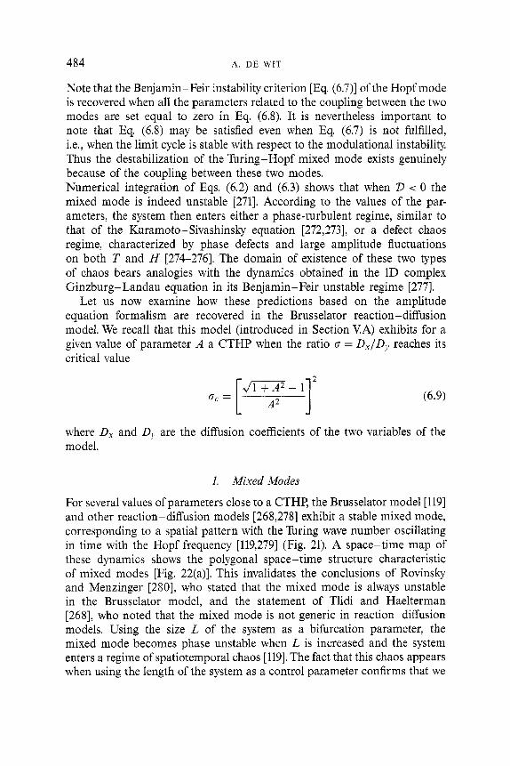
484 A . DE WIT
Note that the Benjamin-Feir instability criterion [Eq. (6.7)] of the Hopf mode is recovered when all the parameters related to the coupling between the two modes are set equal to zero in Eq. (6.8). It is nevertheless important to note that Eq. (6.8) may be satisfied even when Eq. (6.7) is not fulfilled, i.e., when the limit cycle is stable with respect to the modulational instability Thus the destabilization of the Turing-Hopf mixed mode exists genuinely because of the coupling between these two modes. Numerical integration of Eqs. (6.2) and (6.3) shows that when 2) < 0 the mixed mode is indeed unstable [271]. According to the values of the par- ameters, the system then enters either a phase-turbulent regime, similar to that of the Kuramoto-Sivashinslcy equation [272,273], or a defect chaos regime, characterized by phase defects and large amplitude fluctuations on both T and H [274-2761. The domain of existence of these two types of chaos bears analogies with the dynamics obtained in the ID complex Ginzburg-Landau equation in its Benjamin-Feir unstable regime [277].
Let us now examine how these predictions based on the amplitude equation formalism are recovered in the Brusselator reaction-diffusion model. We recall that this model (introduced in Section YA) exhibits for a given value of parameter A a CTHP when the ratio c = D,/D, reaches its critical value
where D, and D, are the diffusion coefficients of the two variables of the model.
1. Mixed Modes
For several values of parameters close to a CTHP, the Brusselator model [119] and other reaction-diffusion models [268,278] exhibit a stable mixed mode, corresponding to a spatial pattern with the Turing wave number oscillating in time with the Hopf frequency [119,279] (Fig. 21). A space-time map of these dynamics shows the polygonal space-time structure characteristic of mixed modes [Fig. 22(a)]. This invalidates the conclusions of Rovinslcy and Menzinger [280], who stated that the mixed mode is always unstable in the Brusselator model, and the statement of Tlidi and Haelterman [268], who noted that the mixed mode is not generic in reaction-diffusion models. Using the size L of the system as a bifurcation parameter, the mixed mode becomes phase unstable when L is increased and the system enters a regime of spatiotemporal chaos [119]. The fact that this chaos appears when using the length of the system as a control parameter confirms that we

SPATIAL PATTERNS AND SPATIOTEMPORAL DYNAMICS 485
Space
(a)
x
Time
ibi
Figure 21. A Turing-Hopf mixed mode observed in a 1D Brusselator model in a system of length 64 with periodic boundary conditions: A = O&D, = l , l l , D , = 10, and B = 1.675. (a) The spatial profile taken at one given time. The spatial structure corresponds to a Turing pattern with wavenumber k,. (b) Periodic temporal dynamics at one given fixed point of the sys- tem, showing oscillations with the Hopf frequency w,
(a)
Figure 22. A space-time map of the three types of mixed modes existing near a CTHP, dis- playing the ID spatial dynamics in the Brusselator model versus time running upward. (a) Turing-Hopf mixed mode with A = 0.8, D, = 1.11, D, = 10, and B = 1.675; (b) subharmonic Turing mode with A = 3, D, = 5.1949, D,, = 10, and B = 10.45; (c) subharmonic Turing-Hopf mode with A = 3, D, = 5.71, Dy = 10, and B = 11.
are dealing with the predicted long-wavelength instability and not with a homoclinic type of chaos. Such spatiotemporal chaos obtained close to a CTHP may be relevant to experimental observations in gas discharges [281] or to those observed in the CIMA reaction [64,92]. It might also be the mechanism leading to chemical turbulence numerically obtained in an enzymatic reaction-diffusion system [282]. Complex mixing of different spa-
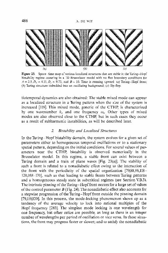
486 A . DE WIT
in) fbi ((.I Figure 23. Space-time map of various localized structures that are stable in the Turing-Hopf bistability regime occuring in a 1D Brusselator model with no flux boundary conditions for A = 2.5, D, = 4.11, Dy = 9.73, and B = 10. Time is running upward. (a) Turing-Hopf front: (b) Turing structure imbedded into an oscillating background; (c) flip-flop.
tiotemporal dynamics are also obtained: The stable mixed mode can appear as a localized structure in a Turing pattern when the size of the system is increased [119]. This mixed mode, generic of the CTHP, is characterized by one wavenumber k, and one frequency o, Other types of mixed modes are also observed close to the CTHP, but in such cases they occur as a result of subharmonic instabilities, as will be described later.
2. Bistability and Localized Structures
In the Turing-Hopf bistability domain, the system evolves for a given set of parameters either to homogeneous temporal oscillations or to a stationary spatial pattern, depending on the initial conditions. For several values of par- ameters near the CTHP, bistability is observed numerically in the Brusselator model. In this regime, a stable front can exist between a Turing domain and a train of plane waves [Fig. 23(a)]. The stability of such a front is related to a nonadiabatic effect owing to the interaction of the front with the periodicity of the spatial organization [79,88,98,118- 120,168-1701, such as that leading to stable fronts between Turing patterns and a homogeneous steady state in subcritical regimes (see Section V.B.3). The intrinsic pinning of theTuring-Hopf front occurs for a large set of values of the control parameter B (Fig. 24). The nonadiabatic effect also accounts for a stepwise progression of the Turing-Hopf front outside the pinning domain [79,119,120]. In this process, the mode-locking phenomenon shows up as a tendency of the average velocity to lock into rational multiples of the Hopf frequency [283]. The simplest mode locking is one wavelength for one frequency, but other ratios are possible, as long as there is an integer number of wavelengths per period of oscillation or vice versa. In these situa- tions, the front may progress faster or slower; and to satisfy the nonadiabatic

SPATIAL PATTERNS AND SPATIOTEMPORAL DYNAMICS 487
Flip-flop
8 10 12 14 16 18
Figure 24. Stability domain ofvarious localized Turing structures imbedded inside a Hopf back- ground versus the control parameter B. The parameters are those given in Figure 23. If the loca- lized Turing pattern contains more than four wavelengths, the nonadiabatic effect is dominant, and the pinning zone limited by the two vertical lines is the same as that for the front. Beyond this pinning band, the only stable localized Turing patterns are those that have a small enough core (less or equal to four wavelengths) for nonvariational interactions to come into play. The localized structure stable in the widest domain is the flip-flop.
constraint, the system then sometimes creates temporary localized subzones [119]. Recently, the velocity of such Turing-Hopf fronts has been studied in detail by Or-Guil and Node [283a].
Two interacting fronts may then build up droplets of one global state imbed- ded into another [ 174-1781. The juxtaposition of twoTuring-Hopf fronts leads to stable localized droplets of a Turing (Hopf) state imbedded into a Hopf (Turing) domain [Fig. 23(b)].We observe that, if theTuring core contains sev- eral wavelengths, the stability domain of such localized structures is the same as that of the front (Fig. 24); and their stabilization can correspondingly be ascribed to nonadiabatic pinning effects, as in the case of the simple front. If the localized Turing domain contains few wavelengths, this stabilizing non- adiabatic effect can no longer be invoked alone. Stable localized Turing pat- terns with few wavelengths are nevertheless observed in the Brusselator model; and the fewer wavelengths they contain, the larger their stability domain. Thus their stability results from nonvariational effects that in other systems [284-2871 stabilize localized structures if they provide a repul- sive interaction between two fronts that otherwise attract each other [19,174,175,288]. They can, therefore, account for the existence of localized dro- plets of one state imbedded :into the other state. This effect is strongest for the so-called flip-flop localized pattern with the smallest core [Fig. 23(c)] and, therefore, the widest stability domain (Fig. 24). This could explain why the flip-flop is the only localized pattern to be observed experimentally in the CIMA reaction for concentration values near the CTHP [64] (Fig. 5).

488 A . DE WIT
Turing-Hopf localized structures have also been observed experimentally in 1D arrays of resistively coupled nonlinear LC oscillators [265] and in binary fluid convection [262].
Bistability between theTuring and Hopf modes near a CTHP had long been predicted in the amplitude equation formalism [ 1551. Recent studies have shown that in this bistability regime, localized structures of one state embed- ded into the other can be stabilized by a combination of nonadiabatic and nonvariational effects [118-1201.
B. Subharmonic Instabilities
When numericul integration of reaction-diffusion models are carried out near a CTHP, scenarios [119,278] occur that do not fit in the bihrcation dia- grams of Figure 20 predicted by the amplitude equations Eqs. (6.2) and (6.3) for the coupled Turing and Hopf modes. Jn particular, two new mixed modes are observed that contain more than one wavenumber. Fourier transforming these spatiotemporal dynamics point out the presence of subharmonic modes of both Turing and Hopf states. These subharmonic modes can be excited because of subharmonic instabilities of the pure Turing and Hopf modes. Indeed, if the bihrcation parameter near the
51 . -.
Figure 25. Dispersion relations explaining the resonances between theTuring and Hopf modes, with their subharmonic in the vicinity of a CTHP. Theplain line and dashedline represent the real and imaginary part, respectively, of the eigenvalues of the linear stability analysis. (a) The sub- harmonic k / 2 of the Turing wavenumber k corresponds to an eigenvalue with a nonvanishing frequency w(k/2). The coupling between the Turing mode and its subharmonic leads to a sub- harmonic Turing mode with two wavenumbers k, k / 2 and one frequency w(k/2). (b) The sub- harmonic w/2 of the Hopf mode is a wave with wavenumber k(w/2). If this wavenumber is on the order of the subharmonic of the Turing wavenumber 2k, then resonance between the Hopf mode, its subharmonic, and the Turing mode leads to a subharmonic Turing-Hopf mode with two wavenumbers k(o/2) , 2k and two frequencies w, w/2.

SPATIAL PATTERNS AND SPATIOTEMPORAL DYNAMICS 489
CTHP is increased, conditions are often such that the root of the characteristic equation corresponding to the subharmonic of the Turing mode, with wave- number k,/2, crosses the imaginary axis (i.e., this mode becomes active), and its imaginary part iw is different from zero, i.e., o(kJ2) # 0 [Fig. 25(a)]. Therefore, the subharmonic mode lies in the Hopf part of the linear dispersion relation. A resonance can then occur between the Turing mode with a wavenumber-frequency couple (k,, 0) of amplitude T and its subhar- monic mode (k,/2, w[k,/2]) corresponding to left and right traveling waves of amplitude AR and AL [289]. The concentration field is then described as
where j y L and W, are the critical eigenvectors corresponding to the left- and right-going waves of wave number kc/2 and frequency w(k,/2) The coupled amplitude equations for the modes read [ 119,290-2921
(6.12)
A linear stability analysis of the solutions to this set of equations shows that for some values of coefficients a mixed standing wave mode (T # 0, A R = AL # 0), characterized by two wavenumbers k,, k,/2 and one frequency o(kc/2b can bifiu-cate from the pure Turing mode (T # 0, A R = AL = 0) [291]. This situation corresponds to one of the mixed modes observed in the Brusselator 11191 [Fig. 22(b)] and in the Gray and Scott model [293]. It also describes oscillating subharmonic pat- terns observed experimentally in the flow of a viscous fluid inside a partially filled rotating horizontal cylinder [263,264]. This subharmonic Turing mode can hrthermore become phase unstable [291], giving rise to spatiotem- poral chaos, as seen in the hydrodynamics experiments.
A subharmonic instability can also affect the Hopf mode (0, we) when it interacts with its subharmonic mode k(o,/2), oc/2. A theoretical analysis
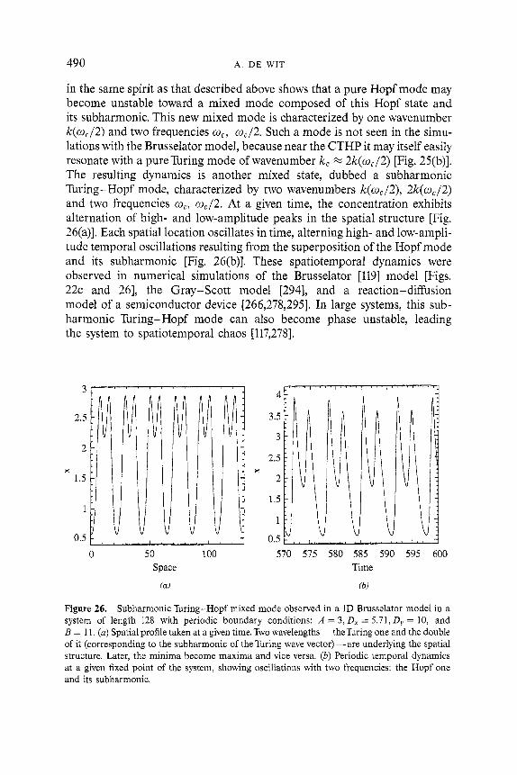
490 A . DE WIT
in the same spirit as that described above shows that a pure Hopf mode may become unstable toward a mixed mode composed of this Hopf state and its subharmonic. This new mixed mode is characterized by one wavenumber k(coJ2) and two frequencies wC, wc/2. Such a mode is not seen in the simu- lations with the Brusselator model, because near the CTHP it may itself easily resonate with a pure Turing mode of wavenumber k, 2k(wC/2) [Fig. 25(b)]. The resulting dynamics is another mixed state, dubbed a subharmonic Turing-Hopf mode, characterized by two wavenumbers k(w,/2), 2k(oc/2) and two frequencies wc, wc/2. At a given time, the concentration exhibits alternation of high- and low-amplitude peaks in the spatial structure [Fig. 26(a)]. Each spatial location oscillates in time, alterning high- and low-ampli- tude temporal oscillations resulting from the superposition of the Hopf mode and its subharmonic [Fig. 26(b)]. These spatiotemporal dynamics were observed in numerical simulations of the Brusselator [119] model [Figs. 22c and 261, the Gray-Scott model [294], and a reaction-diffusion model of a semiconductor device [266,278,295]. In large systems, this sub- harmonic Turing- Hopf mode can also become phase unstable, leading the system to spatiotemporal chaos [117,278].
4
2.5 3.5
3
2.5
1.5 2
1.5
1
0.5 0.5
3
2
X X
1
0 50 100 570 575 580 585 590 595 600 Space Time
(a) (b)
Figure 26. Subharmonic Turing-Hopf mixed mode observed in a 1D Brusselator model in a system of length 128 with periodic boundary conditions: A = 3, D, = 5.71, D, = 10, and B = 11. (a) Spatial profile taken at a given time. Two wavelengths - the Turing one and the double of it (corresponding to the subharmonic of the Turing wave vector) -are underlying the spatial structure. Later, the minima become maxima and vice versa. (b) Periodic temporal dynamics at a given fixed point of the system, showing oscillations with two frequencies: the Hopf one and its subharmonic.

SPATIAL PATTERNS AND SPATIOTEMPORAL DYNAMICS 491
C. Genericity
To summarize, four main types of 1D spatiotemporal dynamics are commonly encountered near a CTHP:
1. Turing-Hopf bistability, which leads to various localized structures, such as the flip-flop.
2. ATuring-Hopf mixed mode, a pureTuring structure oscillating in time with the Hopf frequency
3. A subharmonic Turing mode, a spatial structure with two wavenumbers and one frequency.
4. A subharmonic Turing-Hopf mode, which leads in the vicinity of a Turing bifurcation, to structures with two wavenumbers and two fre- quencies.
In the Brusselator model, these dynamics were classified in an A versus o/gc parameter space (Fig. 27). Here it is important to recall that in the Brusselator model, the frequency of Hopf temporal oscillations is equal to the value of the parameter A, which thus fixes the time scale of the system. Similarly, g relates to the diffusion coefficients that fix the space scale. Figure 27 displays a time scale versus a space scale parameter space. An anal- ogous classification has been performed for the spatiotemporal dynamics occurring in a reaction- diffusion model that describes semiconductor trans- port near a CTHP [278]. In that system, Turing-Hopf bistability (and related localized structures) and the simple and subharmonic mixed modes have been observed as well. In that case the spatiotemporal self-organization is that of the current density rather than that of chemical concentrations. In the semiconductor model, the classification in the time scale versus space scale of the various spatiotemporal dynamics near the CTHP presents strong similarities with the one shown for the Brusselator model.
We propose, therefore, that a time-scale versus length-scale diagram might be an appropriate way for organizing the comparison with other models that present CTHP, because it separates the different scales that reflect the spatial character of the Turing mode and temporal character of the Hopf mode. In this sense, this type of diagram might be usehl for looking for the predicted spatiotemporal dynamics characteristic of an interaction between a steady instability (not necessarily theTuring one) and a Hopf instability. In particular, in nonlinear optics, Turing-Hopf bistability and related localized structures [267] as well as the Turing-Hopf mixed mode [267,268] were identified close to codimension-twoTuring-Hopf points. We believe that the subharmo- nic mixed modes could also be found in the parameter space of these non- linear optical systems using the above classification.

492 A. DE WIT
Turing
a HOPf O T-MM-H A T-B-H A H-B-T 0 H-MM-T
0 SubT 4 SubHT
A
0 0
0 0
rn
A
0
rn
+ +
+ + A
A
a a
0 0
I I I
0.8 1 .o 1.2 OiOC
Figure 27. Summary of the various bifurcation scenarios observed for the Brusselator model and classified in the parameter space A versus a/uc. B stands for Turing-Hopf bistability (with the corresponding localized structures), MM relates to the Turing-Hopf mixed mode (characterized by the wavevector k, and the frequency 0,). The subharmonic Turing mode with two wavevectors k,, k , / 2 and one frequency w, is designated by sub T; the subharmonic Turing-Hopf mode with two wavevectors k,, k,/2 and two frequencies o,, w,/2 is designated by sub HT The succession T-MM-H, for example, means that, when increasing the bifurcation parameter for the given A , cr/crc couple, successive transitions between pure Turing patterns, a mixed mode, and Hopf oscillations are observed. When cr/cr, z 1, the first solution to appear beyond the critical point is a Hopf mode, whereas the Turing mode is dominant at criticality when cr/cr, < 1.

SPATIAL PATTERNS AND SPATIOTEMPORAL DYNAMICS 493
D. Two-Dimensional Spatiotemporal Dynamics
All the Turing-Hopf spatiotemporal dynamics predicted in 1D systems have equivalents in 2D systems. Beyond the pure Turing and pure Hopf solutions, the Turing-Hopf interaction can lead to 2D mixed modes, such as stripes and hexagons, oscillating homogeneously in time with one frequency or to bistability between Turing patterns and a Hopf homogeneous temporal oscil- lation [9,119,296]. In the bistability regimes, Jensen and co-workers [120,121] showed that aTuring dot at the tip of a 2D spiral obtained numeri- cally in the Lengyel-Epstein model is the equivalent of the 1D well-studied flip-flop [64,100]. Such a Turing-Hopf spiral was observed experimentally [48,92,98]. Localized structures with more than one Turing dot are difficult to obtain, because in 2D, pinning of aTuring-Hopf front owing to the under- lying interaction of the front with the pattern occurs only in some privileged directions. This explains why fronts between 2D Turing structures with several wavelengths and an oscillating zone have been obtained only as transients up to now (Fig: 28). Pure 2D Turing-Hopf mixed modes involving only one wavenumber and one frequency have, to our knowledge, never been observed experimentally or numerically, although they should probably be stable for some values of parameters.
On the contrary, the other main types of spatiotemporal dynamic charac- teristics of the Turing-Hopf interaction, i.e., subharmonic instabilities, arise in 2D simulations of the Brusselator model for parameter values close to a CTHP (Fig. 29). In that case, hexagons or stripes oscillate in time with two frequencies. The hexagonal dots have a little bump in their cen- ter, which correspond to the intermediate minima observed in the case of the 1D subharmonic Turing mode [Fig. 26(a)] and are the signature of subhar-
(a) (6)
Figure 28. (a) Transient front between 2D Turing structures and a Hopf oscillating zone observed in the Brusselator model for A = 2.5, D, = 4.49, Dy = 8.91, and B = 8.6 in a system of size 256 x 256 with no flux boundary conditions. The asymptotic state of the system was highly irregular spatiotemporal dynamics. (b) Here B = 11. The 2D spirals are obtained for the same parameter values that give rise to 1D flip-flops.

494 A . DE WIT
X
(c)
Figure 29. The 2D subharmonic Turing-Hopf modes observed in the Brusselator model for A = 2.5, D, = 4.49, and D, = 8.91 in a system of size 256 x 256 with no flux boundary con- ditions. (a) Here B = 7.5. The highly 2D irregular hexagonal-type patterns shown at a given time. Each spot features a little local minimum in its center, indicating the presence of subhar- monics. (b) Here B = 7.8. The 2D stripes shown at a given time. Each band also exhibits a little local minimum in its middle. In both (a) and (b) , each point of the system oscillates in time with two frequencies, as can be seen in the space-time map, showing the dynamics along one line parallel to the y-axis in part (b) versus time running upward. This space-time map is reminiscent of Figure 22(c), evidencing the spatiotemporal dynamics characteristic of a 1D subharmonic Turing-Hopf mixed mode.
monics. The stripes also present analogous little wiggles in their maxima. This behavior can be clearly seen in Figure 29(c), which displays a space-time map of the dynamics along one line of the 2D spatial system. This space-time map is reminiscent of the one characterizing the 1D subharmonic Turing-Hopf mixed mode with two wavenumbers and two frequencies [119] [Fig. 22(c)]. It is however not clear yet which spatial and temporal subharmonics are involved when more than one basic wave vector is present, as in the case of hexagons [297].
Earlier we saw that phase instabilities of the various Turing-Hopf mixed modes may lead to spatiotemporal chaos in 1D [271,291]. Chaotic 2D dynam- ics have often been observed experimentally [48,69,92] and numerically

SPATIAL PATTERNS AND SPATIOTEMPORAL DYNAMICS 495
[ 119,121,2951 in the vicinity of a codimension-two Turing-Hopf point, but no characterization of the destabilizing instabilities have been provided. The study of the 2D Turing-Hopf spatiotemporal dynamics is thus still in its infancy
In several systems, the Turing-Hopf interaction implies a Hopf mode with a nonzero wavenumber [256,258,298]. In that case, the number of possible resonances between the Turing and Hopf wavenumbers become much more important. These resonances provide interesting new 2D dynamics, such as winking hexagons [299], drifting rhombs [300], or hexagons [301], and even quasicrystalline patterns [302,303].
We saw that characteristics of the patterns emerging in a monostable reac- tion-diffusion system are greatly affected by the vicinity of another competing bifurcation, such as the Hopf one. The main advantage of chemical systems is that they allow competition with a bifurcation between different homogeneous steady states. Let us now examine which type of spatiotemporal dynamics such an interplay may induce.
VII. BISTABLE SYSTEMS
The labyrinthine patterns observed in the FIS reaction [129-1311 call for insight into pattern formation in bistable systems. Indeed, bistability between two homogeneous steady states (HSS) characterizes the parameter space in which the FIS spatial structures are obtained. Several other pattern-forming systems, such as gas discharges [37,304], liquid crystals [305], and nonlinear optics [24,164,306], also exhibit bistable regimes. In bistable systems, patterns can result fromTuring bifurcations of different homogeneous branches or from morphological instabilities of fronts connecting different HSS. Let us succes- sively examine these two possibilities.
A. Zero Mode
In bistable systems, patterns can emerge through Turing instabilities on the various HSS branches. Recently, some studies focused on the pattern selection problem using the bistable FitzHugh-Nagumo model [27,307,308] or the Gray and Scott model [293,309]. Two situations leading to bistability are a pitchfork bifurcation (generally imperfect) from one HSS toward two different HSS or an hysterisis loop formed by two back-to-back saddle-node bifurca- tions, as encountered in the FIS system. The study of the pattern selection can be carried out in the vicinity of the cusp point of these transitions. This analysis relies on the fact that the homogeneous perturbations are quasi neutral. As a consequence, a zero mode becomes active and must be taken into account in the dynamics. If some of the HSS undergo diffusive instabilities, it is expected that for some values of parameters the Turing

496 A. DE WIT
and homogeneous bifurcations can interact. In that case, the concentration field C is constructed as
N - C(r, t) = c0 + TOPV~ + C [TjeikI" + ~ j * e - ' ~ ~ ' ' ] w + o(. . .> (7.1)
j = 1
where wo and w are the eigenvectors of the Jacobian matrix of the homo- geneous and distributed systems, respectively The pattern selection problem is then ruled by coupled amplitude equations for TO and the 7;.. The coupling with the zero mode has a profound influence on the possible bifurcation sce- narios. In lD, it can give rise to a rich variety of subharmonic and superhar- monic patterns [310] and even to spatial chaos [311]. In 2D, the corresponding amplitude equations are [32,225]
-g2[IT212 + IT3l2]T~ -g3T1$ -g4ToT,*T,* (7.3)
where PI , P2, g3, and g4 are taken to be positive and kl + k2 + k3 = 0. The equations for T2 and T3 are obtained by cyclic permutations of the subscripts in Eq. (7.3). These equations admit the following classes of solutions:
1. Homogeneous solutions T," given byf( T,O) = 0 with Ti = 0 correspond- ing to the reference HSS of the bistable regime.
2. Mixed spatial pattern solutions with smectic (Ti f 0,l TI I # 0 , T2 = T3 = 0) or hexagonal symmetry (Tt # 0, I TI 1 = I T*l = 1 T3 1 # 0).
It is important to note here that pure stripes or hexagons are generally not solutions to the problem. Moreover, the presence of the amplitude of the homogeneous mode in the pseudo quadratic term v = g4 TI - CI of the ampli- tude Eq. (7.3) for theTuring modes has several consequences for pattern selec- tion. First of all, the sum of the phases 0 = 81 + 02 + 03 of the spatial component of the hexagons depends on the sign of TO, the amplitude of the homogeneous component of the spatial pattern, because it now obeys an equation of the type
dO - dt - (gilTgh - x> sin o (7.4)
The phase 0 relaxes to zero or rc, depending on whether (g4T,h - x ) is < 0 or > 0, respectively, forming HO or Hn mixed hexagons that may even coexist.

SPATIAL PATTERNS AND SPATIOTEMPORAL DYNAMICS 497
Figure 30. Front between HO and Rn hexagons observed in a numerical integration of the FitzHugh-Nagumo model for conditions such that a Turing instability occurs in the vicinity of a bifurcation between different honiogeneous steady states. From Ref. [loll.
In this latter case, fronts between HO and Hrt hexagons can be sustained (Fig. 30). Such fronts have been observed experimentally in convection with SF6 near its critical point [312] and in oscillated granular layers [161]. As Ti is modified when varying the bifurcation parameter, it may bring about a change of sign of the overall quadratic term v, leading to possible re-entrance of hexagons, as observed in liquid crystals [305] or in a gas discharge exper- iment [304]. In 3D systems, the same process applies, and re-entrant BCC or HPC phases are also obtained [225], leading to bifurcation diagrams similar to those obtained for block copolymers [313]. Note that this re- entrance should not be confused with the model-dependent re-entrance that occurs when the nonlinear terms vary with the bifurcation parameter [84,86] (see SectionV.B.2). The re-entrance from a zero mode is more generic and occurs as soon as theTuring instability arises in the vicinity of bifurcations among different HSS. The fact that the quadratic term is a function of TO also leads to the large subcritical appearance of the various planforms and, as a consequence, to possible localized structures, such as 2D hexagonal domains of HO or Hrt embedded into the uniform state [99]. More strikingly, if = 0, the vicinity of a bifurcation toward HSS can give rise to the stabi- lization beyond the stripes of both hexagonal phases, even in systems exhi- biting inversion symmetry [27,225,314].

498 A . DE WIT
The possible bifurcation scenarios in bistable systems can thus be different from those occuring in the absence of the zero mode. Let us also note that, in bistable systems, the amplitude of the mixed Turing-homogeneous mode patterns is on the order of the difference in amplitudes between the two HSS and is thus usually quite large. In some cases, isolated branches of such patterns can form [307,308], and the corresponding high amplitude structures can then be reached only by local finite perturbations applied to the HSS as observed in the FIS experiment [ 1291. Such perturbations gen- erate fronts connecting the two HSS. If such a front now undergoes a mor- phologic instability, the system may evolve toward the isolated Turing branch and settle down as a high-amplitude stationary labyrinthine or hex- agonal pattern, as observed in numerical simulations of the FitzHugh- Nagumo model [151]. In addition to the labyrinthine structures oberved by Lee and co-workers [129], this could also explain experimental obser- vations with the CDIMA system conducted near a cusp point in the mono- stable regime in the vicinity of two different HSS. There, a flowerlike structure develops when a circular front between the two HSS is unstable because of a morphologic instability The flower petals successively break into a hexagonal pattern, which is the asymptotic state of the system [80].
B. Morphologic Instabilities
Many studies have been devoted to the properties of fronts linking two HSS in bistable systems [26,274,315-3171. If the system is composed of at least two species with sufficiently different diffusion coefficients, planar fronts can become unstable, because of morphologic instabilities that lead to a defor- mation of the interface between the two HSS [274,315]. When two fronts come close together, repulsion at short distances occurs, excluding fusion or breakup of the fronts and leading to labyrinthine patterns [129-1311. Numerous theoretical works focused on such instabilities that give rise to fronts and patterns of this type [26,138,174,318-3301.
In such systems, a wealth of different spatiotemporal dynamics is observed, depending on the ratios between the characteristic time and space scales of the activator and inhibitor of the system [26,318,319]. For example, an investigation of the front dynamics in bistable systems was performed in both the fast inhibitor limit [26,318,320] and the slow inhibitor limit [321-3241. The models commonly used in these investigations on reaction-diffusion systems are the bistable FitzHugh-Nagumo-type models [26,138,156,157,319,324,325], the Gaspar-Showalter model of the FIS reaction [130,135,137], and the Gray-Scott model. This last model has allowed, among other things, detailed study of the spot replication process [ 130,131,136-138,293,309,319,326,331-3331.
To account for the properties of labyrinthine structures observed in the FIS reaction, several complementary approach& have been used, such as a general

SPATIAL PATTERNS AND SPATIOTEMPORAL DYNAMICS 499
asymptotic theory of instabilities for patterns with sharp interfaces [328], interfacial dynamic approaches [321,328,329], and parity-breaking bifurca- tions of planar fronts [138,324,330].
VIII. CONCLUSIONS AND PERSPECTIVES
The study of chemical temporal oscillations started with Belousov's experi- mental observations of the now well-known Belousov-Zhabotinskii reaction [42], which was skeptically received by the scientific community [334]. It was only in the 1970s that the number of works devoted to these temporal oscillations took off [7,42,43]. Today, oscillating reactions are a classical domain of nonlinear science and are recognized as a key element in the under- standing of several biorythms [335]. They are now being considered in the engineering domain for applications such as temporally modulated drug release [336,337] and possible digital logic [338].
Spatial chemical patterns may now be on their way to an analogous history Turing structures were predicted theoretically quite a long time ago; and the recently experimentally observed structures have led to many studies devoted to spatial chemical patterns and related spatiotemporal dynamics. Nevertheless, more work is needed to unravel the richness of these spatial chemical structures.
First, several aspects of the experimentally obtained Turing patterns call for additional studies, such as the 3D pattern selection problem. The fact that the Turing wavelength is intrinsic places reaction- diffusion systems in a unique position among pattern-forming systems for studying all possible 3D self-organizations, which are much richer than in 2D systems [117]. Unavoidably related to that is the problem of gradients and how spatial vari- ation of parameters affects the selection and orientation of spatial structures. Another area of chemical systems is the interaction with other instabilities. The Turing-Hopf coupling provides very rich spatiotemporal dynamics, which are now being discovered in other systems, such as nonlinear optics [267]. It is expected that several dynamics, such as the subharmonic mixed modes and phase instabilities of the Turing-Hopf mixed modes that lead to spatiotemporal chaos, will soon be discovered in those systems as well. Note that the different mechanisms that give rise to chaotic space-time behaviors near a CTHP provide tools for testing to what extent measures that quantify chaotic dynamics are independent from the instability mechanism in the same system. In addition, the spatiotemporal chaos owing to a phase instability of the various mixed modes is much richer than the chaos in the complex Ginzburg-Landau equation, for instance, because the underlying unstable base state contains different Turing and/or Hopf modes. This fact was exploited by Petrov and co-workers [294], who stabilized

500 A . DE WIT
a spatial pattern and a temporal oscillation out of a chaotic Turing-Hopf mixed mode using chaos-control techniques. In the same spirit, the obser- vation of spatial patterns in bistable reaction-diffusion systems has shown that the pattern selection problem can be affected in the bistability regime by the presence of a homogeneous mode.
The analysis of the coupling between Turing modes with Hopf or homo- geneous modes participate in a stream of studies that enlarge the number of modes considered to play a role in the buildup of spatial planforms and spatiotemporal dynamics. In the first classical papers devoted to the Rayleigh-Benard instability [77,207] and in many papers that focused on spatial patterns, the only structures considered were stripes, squares, and hexagons. Experiments have shown, however, that more spatial modes some- times need to be considered already in 2D systems, as in the case of quasi- crystalline structures observed in the Faraday instability [ 143,1441 and in non- linear optical systems [145]. Other structures built on the whole circle of unstable modes, such as turbulent crystals [339], have also been described. In addition, modes of different lengths may sometimes coexist [340] or res- onate to yield nonequilateral patterns, black-eyes, decagons, etc. [ 191,3411. In the same spirit, the coupling between a nonoscillatory short-wavelength instability and a long-wavelength neutrally stable mode was recently shown to produce new spatiotemporal dynamics intermediate between those of the traditional long- and short-wavelength ones [342,343]. Oscillatory modes with a finite wavenumber are also able to lead to pat- tern-forming dynamics in reaction- diffusion systems, such as traveling and standing waves and target patterns in 1D systems [344-3461. In 2D sys- tems, resonance interactions among several pure Hopf waves produce a multi- plicity of patterns, including traveling and blinking rolls, rhombs, and hexagons [301,347,348]. All these possibilities are potentially viable in chemi- cal systems and remain topics of future research.
Beyond the complexity related to the increasing number of modes con- sidered, one must also deal with the complexity arising from heterogeneities and anisotropies. Voroney and co-workers [349] analyzed the effect of spatial inhomogeneities in the distribution of complexing agents on Turing patterns and their switch toward oscillating behaviors. Such a distribution arises if one assumes that diffusion coefficients are space dependent owing to the geometry of the medium [350] or to an imposed spatial distribution of the color indicator in the CIMA system, as was done for the study of waves in patterned systems [351]. This could allow for an understanding of the interplay between the wavelength of the pattern and the typical length scale of the inhomogeneities that sometimes leads to time-dependent sol- utions [349,352,353]. Such possible coupling is connected with the interaction of different spatial modes alluded to above.

SPATIAL PATTERNS AND SPATIOTEMPORAL DYNAMICS 501
In the same spirit, Turing patterns can be affected by anisotropies, such as those arising from gradients [85], electrical fields [93,125,354-3561, and aniso- tropic diffusion coefficients [357]. An important source of anisotropies is hydrodynamic flows. In the past, hydrodynamic effects prevented the obser- vation of Turing patterns [358,359]. Now that the conditions for obtaining Turing structures in gels to avoid any perturbing hydrodynamic current are better understood, possible competition of Turing structures with flows can be studied. Two different situations occur, depending on whether hydrodynamic currents are of internal or external origins. Internal currents may arise owing to chemically driven convection. In gel-free media [63], the density gradients inherent to the spatial variation of concentrations in the Turing pattern can generate local convective motions [360-3621. External currents refer to global flows imposed along a given direction as the result of gradients of pressure or shearing, which lead to advected Turing patterns [196,363-3681. In that case, an absolute and a convective instability [369] of the Turing modes can arise, depending on the flow rate; and the linear stability analysis of the patterns is modified [48,368]. In such systems, one needs to be cautious with the origin of patterns. It is indeed known that noise-sustained spatial structures may emerge in convec- tively unstable regimes [370], which should not be confused with Turing pat- terns. Moreover, systems with reactive flows exhibit differential flow- induced chemical instabilities (DIFICI) [371] that are typically convectively unstable [79]. This traveling wave-forming instability occurs when one reactive is binded to a support and another one flows onto it. Owing to the richness of different pattern-forming mechanisms in advection-reaction-diffusion sys- tems and the possible interactions among them [ 193,366,368,372,3731, more work must be done to understand the properties of spatial structures in the presence of flows.
Although the Turing instability and the Rayleigh-Benard instabilities have been the paradigms of pattern formation instabilities in chemical and hydro- dynamic systems, respectively, other pattern-forming conditions related to chemical systems have also been studied. For example, Petrov and co-workers [374] recently confirmed experimentally that the external periodic forcing by light of a photosensitive variant of the Belousov-Zhabotinslq reaction can lead to a resonant pattern formation, which was predicted theoretically by Coullet and Emilsson [ 179,1801. Another source of pattern formation is global coupling, which plays an important role in some reaction-diffusion systems. Global coupling arises as a limiting case of infinite diffusivity of one of the variables. The temporal evolution equation of this variable is then given by an integral equation of the type xt = ( f ( x , y ) ) , where (...) denotes averaging over the entire reactive domain. Such a global control is encountered, e.g., in experiments with catalytic wires [375,376], in which

502 A . DE WIT
global coupling results from a constant mean temperature. Similarly, conser- vation of the total current leads to a global control in electrochemical [377] and glow discharge devices [286]. In such systems, propagating waves owing to oscillatory local kinetics are transformed into standing waves by global coupling, which can also lead to complex dynamics of pulses and kinks [285]. Standing waves owing to a global control occur in catalytic reactions as well [ 17,378-3821. There global control is achieved through the gas phase, which mixes the substances and thus imposes a rapid communication among different locations of the catalytic surface and even among different surfaces [383]. Recently, Middya and Luss [384] suggested that the same effect could apply when a reaction-diffusion system operates in a thin slab in contact with a surrounding vessel in which rapid homogeneitization of the concentrations take place. They showed that, if global interaction between the gel and the vessel is taken into account, then spatial patterns can result from the global control, even when reaction-diffusion mechanisms cannot create patterns on their own. In that case, the patterns bear analogies with those observed in the FIS experiments [129,384,385], and transitions between striped and spotted patterns with changing levels of global control can be obtained [384,386].
To conclude, let us say that a movement is under way to complement the analysis of temporal complexity in chemical reactions by their spatial aspect. This evolution toward an increase in complexity is also parallel to an increase of diversity and richness of the possible spatial and related spa- tiotemporal behaviors to be discovered in chemical systems. Chances are, therefore, great that in the near future spatial patterns will provide numerous potential applications wherever a spatial distribution of chemical activity is necessary.
Acknowledgments
I wish to thank Professor G. Nicolis for his continuous support and interest in this work. I am much indebted to Pierre Borckmans and Guy Dewel, in collaboration with whom all my contributions to the field of Turing patterns have been obtained, for numerous enlightening dis- cussions. I thank them for suggesting various modifications of this manuscript. I also acknowledge discussions with I? De Kepper, E. Dulos, J. Boissonade, D. Lima, M’F. Hilali, J. Verdasca, S. Metens, J. Pontes, J. Lauzeral, and D. Walgraef. I thank in particular P. De Kepper for his comments on the manuscript and for providing me with the figures of experimental results. I acknowledge the financial support from the Belgian Federal Office for Scientific, Technical, and Cultural Affairs under the Pales #Attraction Interuniversitaire program.
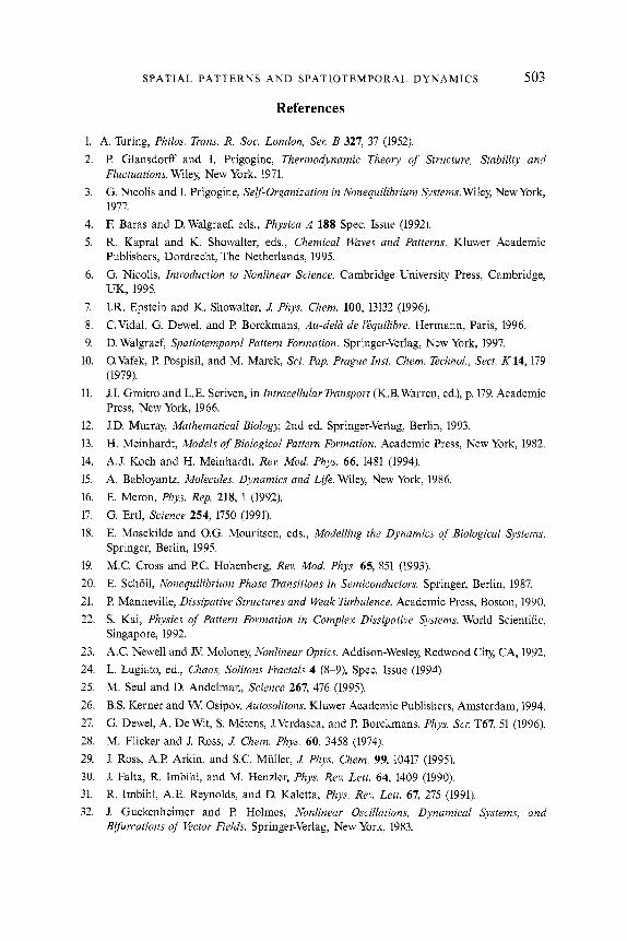
SPATIAL PATTERNS A N D SPATIOTEMPORAL DYNAMICS 503
References
1. A. Turing, Philos. Trans. R. Soc. London, Ser. B 327, 37 (1952).
2.
3.
4.
5.
6.
7.
8.
9.
10.
11.
12.
13.
14.
15.
16.
17.
18.
19.
20.
21.
22.
23.
24.
25.
26.
27.
28.
2 9.
30. 31.
32.
P. Glansdorff and I. Prigogine, Thermodynamic Theory of Structure, Stability and Fluctuations. Wiley, New York, 1971.
G. Nicolis and I. Prigogine, Self-Organization in Nonequilibrium Systems. Wiley, New York, 1977.
E Baras and D. Walgraef, eds., Physica A 188 Spec. Issue (1992).
R. Kapral and K. Showalter, eds., Chemical Waves and Patterns. Kluwer Academic Publishers, Dordrecht, The Netherlands, 1995.
G. Nicolis, Introduction to Nonlinear Science. Cambridge University Press, Cambridge, UK, 1995.
I.R. Epstein and K. Showalter, J Phys. Chem. 100, 13132 (1996).
C.Vida1, G. Dewel, and I? Borckmans, Au-deli de IEquilibre. Hermann, Paris, 1996.
D. Walgraef, Spatiotemporal Pattern Formation. Springer-Verlag, New York, 1997.
O.Vafek, P. Pospisil, and M. Marek, Sci. Pap. Prague h s t . Chem. Technol., Sect. K 14, 179 (1979).
J.I. Gmitro and L.E. Scriven, in Intracellular Transport (K.B. Warren, ed.), p. 179. Academic Press, New York, 1966.
J.D. Murray, Mathematical Biology, 2nd ed. Springer-Verlag, Berlin, 1993.
H. Meinhardt, Models of Biological Pattern Formation. Academic Press, New York, 1982.
A.J. Koch and H. Meinhardt, Rev. Mod. Phys. 66, 1481 (1994).
A. Babloyantz, Molecules, Dynamics and Life. Wile5 New York, 1986.
E. Meron, Phys. Rep. 218, 1 (1992).
G. Ertl, Science 254, 1750 (1991).
E. Mosekilde and O.G. Mouritsen, eds., Modelling the Dynamics of Biological @stems. Springer, Berlin, 1995.
M.C. Cross and P.C. Hohenberg, Rev. Mod. Phys. 65, 851 (1993).
E. Scholl, Nonequilibrium Phase Transitions in Semiconductors. Springer, Berlin, 1987.
P. Manneville, Dissipative Structures and Weak Turbulence. Academic Press, Boston, 1990.
S. Kai, Physics of Pattern Formation in Complex Dissipative Systems. World Scientific, Singapore, 1992.
A.C. Newel1 and JX Moloney, Nonlinear Optics. Addison-Wesley, Redwood City, CA, 1992.
L. Lugiato, ed., Chaos, Solitons Fractals 4 (8-9), Spec. Issue (1994).
M. Seul and D. Andelman, Science 267, 476 (1995).
B.S. Kerner and W. Osipov, Autosolitons. Kluwer Academic Publishers, Amsterdam, 1994.
G. Dewel, A. De Wit, S . Metens, J.Verdasca, and P. Borckmans, Phys. Scv. T67, 51 (1996).
M. Flicker and J. Ross, J . Chem. Phys. 60, 3458 (1974).
J. Ross, A.P. Arkin, and S.C. Muller, J Phys. Chem. 99, 10417 (1995).
J. Falta, R. Imbihl, and M. Henzler, Phys. Rev. Lett. 64, 1409 (1990).
R. Imbihl, A.E. Reynolds, and D. Kaletta, Phys. Rev. Lett. 67, 275 (1991).
J. Guckenheimer and I? Holmes, Nonlineav Oscillations, Dynamical Systems, and Bifurcations of Vector Fields. Springer-Verlag, New York, 1983.

504 A . DE WIT
33. S.K. Scott, Chemical Chaos. Clarendon Press, Oxford, 1991. 34. A.C. Newell, T. Passot, and J. Lega, Annu. Rev. Fluid Mech. 25, 399 (1993). 35. L. Szili and J. Toth, Phys. Rev. E 48, 183 (1993). 36. J.A.Vastano, J.E. Pearson,W Horsthemke, and H.L. Swinney, Phys. Lett. A 124,320 (1987). 37. C. Radehaus, H. Willebrand, R. Dohmen, E-J. Niedernostheide, G. Bengel, and H.-G.
Purwins, Phys. Rev. A 45, 2546 (1992). 38. F.-J. Niedernostheide, M. Ardes, M. Or-Guil, and H.-G. Purwins, Phys. Rev. B 49, 7370
(1994). 39. K. Krishan, Nature (London) 287, 420 (1980). 40. D. Walgraef and N.M. Ghoniem, eds., Patterns, Defects and Material Instab
Academic Publishers, Dordrecht, the Netherlands, 1990. 41. YJ. Emelyanov, Laser Phys. 2, 389 (1992). 42. R.J. Field and M. Burger, Oscillations and Traveling Waves in Chemical Systems. Wiley, New
York, 1985.
43. J. Ross, S.C. Miiller, and C.Vida1, Science 240, 460 (1988). 44. Z . Noszticzius, W Horsthemke, WD. McCormick, H.L. Swinney, and WY Tam, Nature
(London) 329, 619 (1987).
45. WN. Tam, J.A.Vastano, H.L. Swinney, and W. Horsthemke, Phys. Rev. Lett. 61,2163 (1988). 46. Q. Ouyang, J. Boissonade, J.C. Roux, and I? De Kepper, Phys. Lett. A 134, 282 (1989). 47. Y Castets, E. Dulos, J. Boissonade, and P. De Kepper, Phys. Rev. Lett. 64, 2953 (1990). 48. J. Boissonade, E. Dulos, and €? De Kepper, in Chemical Waves and Patterns (R. Kapral and
K. Showalter, eds.), p. 221. Kluwer Academic Publishers, Dordrecht, the Netherlands, 1995.
49. €? De Kepper, J. Boissonade, and I.R. Epstein, J . Phys. Chem. 94, 6525 (1990). 50. I. Lengyel, G. Rabai, and LR. Epstein, J . Am. Chem. Soc. 112, 4606 (1990). 51. A. Cesaro, J.C. Benegas, and D. R. Ripoll, J . Phys. Chern. 90, 2787 (1986). 52. J. Boissonade, J. Phys. (Paris) 49, 541 (1988). 53. Q. Ouyang and H.L. Swinney, Nature (London) 352, 610 (1991). 54. I. Lengyel, G. Rabai, and I.R. Epstein, J . Am. Chem. Soc. 112, 9104 (1990). 55. I. Lengyel and I.R. Epstein, in Chemical Waves and Patterns (R. Kapral and K. Showalter,
eds.), p. 297. Kluwer Academic Publishers, Dordrecht, the Netherlands, 1995.
56. I.R. Epstein, I. Lengyel, S. Kadar, M. Kagan, and M.Yokoyama, Physica A 188,26 (1992). 57. 1. Lengyel and I.R. Epstein, Science 251, 650 (1991). 58. I. Lengyel and I.R. Epstein, Proc. Natl. Acad. Sci. U X A . 89, 3977 (1992).
59. A. Hunding and P.G. Scerensen, J . Math. Biol. 26, 27 (1988). 60. J.E. Pearson, Physica A 188, 178 (1992). 61. J.E. Pearson and WJ. Bruno, Chaos 2, 513 (1992). 62. Z . Noszticzius, Q. Ouyang,W.D. McCormick, and H.L. Swinney, J . Phys. Chem. 96, 6302
(1 9 92). 63. K. Agladze, E. Dulos, and P. De Kepper, J . Phys. Chem. 96, 2400 (1992). 64. J.-J. Perraud, K. Agladze, E. Dulos, and P. De Kepper, Physica A 188, 1 (1992). 65. K.J. Lee,WD. McCormick, H.L. Swinney, and Z . Noszticzius, J . Chem. Phys. 96, 4048
(1992). 66. Q. Ouyang, R. Li, G. Li, and H.L. Swinney, J . Chem. Phys. 102, 2551 (1995).

SPATIAL PATTERNS AND SPATIOTEMPORAL DYNAMICS 505
67.
68.
69.
70.
71.
72.
73.
74.
75.
76.
77.
78.
79.
Q. Ouyang and H.L. Swinney, Chaos 1, 411 (1991).
Q. Ouyang, Z. Noszticzius, and H.L. Swinney, J . Phys. Chem. 96, 6773 (1992).
B. Rudovics, E. Dulos, and P. De Kepper, Phys. Scr. T67, 43 (1996).
E. Dulos, I? Davies, B. Rudovics, and P. De Kepper, Physica D 98, 53 (1996).
B. Rudovics, Ph.D. Thesis, Bordeaux University, 1995. I? De Kepper,Y Castets, E. Dulos, and J. Boissonade, Physica D 49, 161 (1991).
L.M. Pismen, J . Chem. Phys. 72, 1900 (1980).
H. Haken and H. Olbrich, J . Math. Biol. 6, 317 (1978).
D. Walgraef, G. Dewel, and P. Borckmans, Adv. Chem. Phys. 49, 311 (1982).
S. Ciliberto, P. Coullet, J. Lega, E. Pampaloni, and C. Perez-Garcia, Phyx. Rev. Lett. 65, 2370 (1990).
F.H. Busse, J . Fluid Mech. 30, 625 (1967). L.M. Pismen, in Dynamics of Nonlinear @stems (V. Hlavacek, ed.), p. 47. Gordon & Breach, New York, 1986.
P. Borckmans, G. Dewel, A. De Wit, and D. Walgraef, in Chemical Waves and Patterns (R. Kapral and K. Showalter, eds,), p. 323. Kluwer Academic Publishers, Dordrecht, the Netherlands, 1995.
80. P.W. Davies, P. Blanchedeau, E. Dulos, and P. De Kepper, J . Phys. Chem. A 102,8236 (1998).
81. J. Boissonade,V. Castets, E. Dulos, and P. De Kepper, Int. J . Numer. Math. 97, 67 (1991).
82. T.C. Lacalli, D.A. Wilkinson, and L.C. Harrison, Development (Cambridge, UK) 104, 105 (1988).
83. P. Borckmans, G. Dewel, and A. De Wit, Rev. Cytol. Biol. Eg.-Bot. 14, 209 (1991).
84. IVerdasca, A. De Wit, G. Dewel, and P. Borckmans, Phys. Lett. A 168, 194 (1992).
85. P. Borckmans, A. De Wit, and G. Dewel, Physica A 188, 137 (1992).
86. V. Dufiet and J. Boissonade, J . Chem. Phys. 96, 664 (1992).
87. V. Dufiet and J. Boissonade, Physica A 188, 158 (1992).
88. 0. Jensen,YO. Pannbacker, G. Dewel, and P. Borckmans, Phys. Lett. A 179, 91 (1993).
89. Q. Ouyang, G.H. Gunaratne, and H.L. Swinney, Chaos 3,707 (1993).
90. G.H. Gunaratne, Q. Ouyang, and H.L. Swinney Phys. Rev. E 50, 2802 (1994).
91. Q. Ouyang and H.L. Swinney, in Chemical Waves and Pattevns (R. Kapral and K. Showalter, eds.), p. 269. Kluwer Academic Publishers, Dordrecht, the Netherlands, 1995.
92. €? De Kepper, J.-J. Perraud, B. Rudovics, and E. Dulos, In?. J . Bifurcation Chaos 4, 1215 (1994).
93. M. Watzl and A.F. Miinster, J . Phys. Chem. A 102, 2540 (1998).
94. R.D.Vigi1, Q. Ouyang, and H.L. Swinney, Physica A 188, 17 (1992).
95. I. Lengyel, S . Kadar, and I.R. Epstein, Phys. Rev. Lett. 69, 2729 (1992).
96. M. Herschkowitz-Kaufman and G. Nicolis, J . Chem. Phys. 56, 1890 (1972).
97. J.F. Auchmuty and G. Nicolis, Bull. Math. Biol. 37, 323 (1975).
98. G. Dewel, P. Borckmans, A. DeWit, B. Rudovics, J.-J. Perraud, E. Dulos, J. Boissonade, and P. De Kepper, Physica A 213, 181 (1995).
99. M’E Hilali, S. Mktens, G. Dewel, and I? Borckmans, Phys. Rev. E 51, 2046 (1995). 100. 0. Jensen, E. Mosekilde, I? Borckmans, and G. Dewel, Phys. Scr. 53, 243 (1996).
101. M’E Hilali, Ph.D. Thesis, Brussels University, 1997.

506 A. DE WIT
102. A. De Wit, P. Borckmans, and G. Dewel, in Instabilities and Nonequilibrium Structures IV (E. Tirapegui and W Zeller, eds.), p. 247. Kluwer Academic Publishers, Dordrecht, the Netherlands, 1993.
102a. E. Barillot, PhD Thesis (Bordeaux University, 1996).
103. A. Hunding and M Brans, Physica D 44, 285 (1990).
104. V. Dufiet and J. Boissonade, Phys. Rev. E 53, 4883 (1996).
105. M. Bestehorn, Phys. Rev. E 53, 4842 (1996).
106. P.M. Eagles, Proc. R. SOC. London, Ser. A 371, 359 (1980).
107. L. Kramer, E. Ben-Jacob, H. Brand, and M.C. Cross, Phys. Rev. Lett. 49, 1891 (1982).
108. Y. Pomeau and S. Zaleski, J . Phys. Lett. (Orsay, Fr.) 44, L135 (1983).
109. I.C. Walton, J . Fluid Mech. 131, 455 (1983).
110. M.A. Dominguez-Lerma, D.S. Cannell, and G. Ahlers, Phys. Rev. A 34, 4956 (1986).
111. H. Riecke and H.-G. Paap, Phys. Rev. Lett. 59, 2570 (1987).
112. G. Dewel and P. Borckmans, Phys. Lett. A 138, 189 (1989).
113. B.A. Malomed and A.A. Nepomnyashchy, Europhys. Lett. 21, 195 (1993). 114. J. da Rocha Miranda Pontes, Ph.D. Thesis, Brussels University, 1994.
115. R.B. Hoyle, Phys. Rev. E 51, 310 (1995).
116. R.J. Wiener, G.L. Snyder, M.P. Prange, D. Frediani, and P.R. Diaz, Phys. Rev. E 55, 5489 (1997).
117. A. De Wit, P. Borckmans, and G. Dewel, Proc. Natl. Acad. Sci. U X A . 94, 12765 (1997).
118. J.-J. Perraud, A. DeWit, E. Dulos, P. De Kepper, G. Dewel, and P. Borckmans, Phys. Rev. Lett. 71, 1272 (1993).
119. A. De Wit, D. Lima, G. Dewel, and P. Borckmans, Phys. Rev. E 54, 261 (1996).
120. 0. Jensen,V.O. Pannbacker, E. Mosekilde, G. Dewel, and P. Borckmans, Phys. Rev. E50,736 (1994).
121. 0. Jensen,V.O. Pannbacker, E. Mosekilde, G. Dewel, and P. Borckmans, Open Syst. Inf Dyn. 3, 215 (1995).
122. 1.R. Epstein and I. Lengyel, Physica D 84, 1 (1995).
123. I. Lengyel, S. Kadar, and I.R. Epstein, Science 259, 493 (1993).
124. M. Watzl and A.E Miinster, Chenz. Phys. Lett. 242, 273 (1995).
125. A.E Miinster, M. Watzl, and EVI! Schneider, Phys. Scr. T67, 58 (1996).
126. M. Burger and R.J. Field, Nature (London) 307, 720 (1984).
127. P. Resch, A.E Miinster, and Ec\! Schneider, J Phys. Chem. 95, 723 (1991).
128. YX. Zhang and R.J. Field, J Phys. Chem. 95, 6270 (1991).
129. K.J. Lee,WD. McCormick, Q. Ouyang, and H.L. Swinney, Science 261, 192 (1993).
130. K.J. Lee and H.L. Swinney, Phys. Rev. E 51, 1899 (1995).
131. G. Li, Q. Ouyang and H.L. Swinney, J Chem. Phys. 105, 10830 (1996). 132. E.C. Edblom, M. Orban, and I.R. Epstein, J . Am. Chem. Soc. 108, 2826 (1986). 133. E.C. Edblom, L. Gyorgyi, and I.R. Epstein, J Am. Chem. SOC. 109, 4876 (1987).
134. V. Gaspar and K. Showalter, J . Am. Chem. SOC. 109,4869 (1987). 135. V. GaspAr and K. Showalter, J Phys. Chem. 94, 4973 (1990). 136. K.J. Lee,WD. McCormick, J. Pearson and H.L. Swinney, Nature (London) 369,215 (1994).
137. K.J. Lee and H.L. Swinney, Int. J Bifurcation Chaos 7, 1149 (1997).

SPATIAL PATTERNS AND SPATIOTEMPORAL DYNAMICS 5 07
138. D. Haim, G. Li, Q. Ouyang,WD. McCormick, H.L. Swinney, A. Hagberg, and E. Meron, Phys. Rev. Lett. 77, 190 (1996).
139. J. Swift and P.C. Hohenberg, Phys. Rev. A 15, 319 (1977).
140. F. Hynne and P.G. Saxensen, Phys. Rev. E 40, 4106 (1993).
141. B. Dionne, M. Silber, and A.C. Skeldon, Nonlinearity 10, 321 (1997).
142. B.A. Malomed, A.A. Nepomnyashchy, and M.I. Tribelsb, Sov. Phys.-JETP (Engl. Trans/.) 69, 388 (1989).
143. B. Christiansen, P. Alstrerm, and M.T. Levinsen, Phys. Rev. Lett. 68, 2157 (1992).
144. WS. Edwards and S. Fauve, Phys. Rev. E 47, R788 (1993).
145. E. Pampaloni, P.L. Ramazza, S. Residori, and F.T. Arecchi, Phys. Rev. Lett. 74, 258 (1995).
146. B.A. Malomed and M.I. Tribelsb, Sov. Phys.-JETP (Engl. Transl.) 65, 305 (1987).
147. G. Nicolis, T. Erneux, and M. Herschkowitz-Kaufman, Adv. Chem. Phys. 38, 263 (1978).
148. E. Mosekilde, 0. Jensen, G. Dewel, and P. Borckmans, Syst. Anal. Model. Simul. 18-19,45 (1995).
149. E. Mosekilde, F. Larsen, G. Dewel, and P. Borckmans, Int J . Bifurcation Chaos 8, 1003 (1998).
150. J. Schnackenberg, J . Theor. Biol. 81, 389 (1979).
151. S. Metens, Ph.D. Thesis, Brussels University, 1998.
152. M’E Hilali, S. Metens, G. Dewel, and €? Borckmans, in Instab es and Nonequilibrium Structures V (E. Tirapegui and W Zeller, eds.). Kluwer Academic Publishers, Dordrecht, the Netherlands, 1996.
153. I. Prigogine and R. Lefever, 1 Chem. Phys. 48, 1695 (1968).
154. Y. Kuramoto and T Tsuzuki, Prog. Theor. Phys. 52, 1399 (1974).
155. H. Kidachi, Pvog. Theor. Phys. 63, 1152 (1980).
156. R. FitzHugh, Biophys. J 1, 445 (1961).
157. J. Nagumo, S. Arimoto, and S. Yoshizawa, Proc. IRE SO, 2061 (1962).
158. P. Gray and S.K. Scott, Chem. Eng. Sci. 38, 29 (1983).
159. K. Kumar and K.M.S. Bajaj, Phys. Rev. E 52, R4606 (1995).
160. C. Bizon, M.D. Shattuck, J.B. Swift,WD. McCormick, and H.L. Swinney, Phys. Rev. Lett. 80, 57 (1998).
161. F. Melo, P.B. Umbanhowar, and H.L. Swinney, Phys. Rev. Lett. 75, 3838 (1995).
162. W.J. Firth and A. J. Scroggie, Europhys. Lett. 26, 521 (1994).
163. G. D’Alessandro and WJ. Firth, Phys. Rev. A 46, 537 (1992).
164. T. Ackemann,YA. Logvin, A. Heuer, and W Lange, Phys. Rev. Lett. 75, 3450 (1995).
165. Y. Astrov, E. Ammelt, S. Teperick, and H.-G. Purwins, Phys. Lett. A 211, 184 (1996).
166. E. Ammelt,Y Astrov, and H.-G. Purwins, Phys. Rev. E 55, 6731 (1997).
167. G. Dee and J.S. Langer, Phys. Rev. Lett. SO, 383 (1983).
168. Y. Pomeau, Physica D 23, 3 (1986).
169. D. Bensimon, B.I. Shraiman, and V. Croquette, Phys. Rev. A 38, 5461 (1988).
170. B.A. Malomed, A.A. Nepomnyashchy, and M.I. Tribelsky Phys Rev. A 42, 7244 (1990). 171. E. Ben-Jacob, H. Brand, G Dee, L. Kramer, and J.S. Langer, Physica D 14, 348 (1985). 172. W van Saarloos, Phys. Rev. A 37, 211 (1988).
173. W van Saarloos, Phys. Rev. A 39, 6367 (1989).
508 A. DE WIT
174. S. Koga and Y Kuramoto, Prog. Theor. Phys. 63, 106 (1980). 175. 0. Thual and S. Fauve, J Phys. (Paris) 49, 182 (1988).
176. W van Saarloos and P.C. Hohenberg, Physica D 56, 303 (1992).
177. V. Hakim, l? Jakobsen, and Y Pomeau, Europhys. Lett. 11, 19 (1990).
178. G. Dewel and P. Borckmans, Europhys. Lett. 17, 523 (1992).
179. P. Coullet and K. Emilsson, Physica A 188, 190 (1992).
180. l? Coullet and K. Emilsson, Physica D 61, 119 (1992).
181. AM Gaponov-Grekhov, A.S. iomov, GY Osipov, and M.1 Rabinovich, in Nonlinear Waves 1: Dynamics and Evolution (AM Gaponov-Grekhov, M.I. Rabinovich, and J. Engelbrecht, eds.), Res. Rep. Phys., p. 65. Springer-Verlag, Berlin, 1989.
182. H. Herrero, C. Perez-Garcia, and M. Bestehorn, Chaos 4, 15 (1994).
183. M.D. Graham, I.G. Kevrekidis, K. Asakura, J. Lauterbach, K. Krischer, H.-H. Rotermund, and G. Ertl, Science 264, 80 (1994).
184. C.Varea, J.L. Aragbn, and R.A. Barrio, Phys. Rev. E 56, 1250 (1997).
185. B. von Haeften, G. Izus, R. Deza, and C. Borzi, Physica A 236, 403 (1997).
186. B. Hasslacher, R. Kapral, and A. Lawniczak, Chaos 3, 7 (1993).
187. S. Kondo and R. Asai, Nature (London) 376, 765 (1995).
188. G. Izus, R. Deza, C. Borzi, and H. Wio, Physica A 237, 135 (1997).
189. J.D. Crawford and E. Knobloch, Annu. Rev. Fluid Mech. 23, 341 (1991).
190. V. Perez-Munuzuri, M. Gomez-Gesteira, A.P. Munuzuri, L.O. Chua, and V. Perez-Villar, Physica D 82, 195 (1995).
191. B.A. Malomed, A.A. Nepomnyashchy, and A.E. Nuz, Physica D 70, 357 (1994).
192. R. Kapral, A.T. iawniczak, and l? Masiar, Phys. Rev Lett. 66, 2539 (1991).
193. R. Kapral, Physica D 86, 149 (1995). 194. D. Dab, J.-P. Boon and Y-X. Li, Phys. Rev. Lett. 66, 2535 (1991).
195. S. Ponce Dawson, S. Chen, and G.D. Doolen, J Chem. Phys. 98, 1514 (1993).
196. J.R. Weimar and J.-€? Boon, Physica A 224, 207 (1996). 197. A.C. Newell, T. Passot, C. Bowman, N. Ercolani, and R. Indik, Physica D 97, 185 (1996).
198. C. Bowman and A.C. Newell, Rev. Mod. Phys. 70, 289 (1998). 199. L.M. Pismen and A.A. Nepomnyashchy, Europhys. Lett. 24, 461 (1993).
200. M.I. Rabinovich and L.S. Tsimring, Phys. Rev. E 49, R35 (1993).
201. S. Rica and E. Tirapegui, Phys. Rev. Lett. 64, 878 (1990). 202. L.S. Tsimring and M.I. Rabinovich, Spatio-Temporal Pattern Nonequilib. Complex @st.,
Proc. NATO-ARK Santa Fe, 1993.
203. L.M. Pismen and A.A. Nepomnyashchy, Europhys. Lett. 27, 433 (1994). 204. S. Ciliberto, E. Pampaloni, and C. Pirez-Garcia, J Stat. Phys. 64, 1045 (1991). 205. A.C. Newell and J.A. Whitehead, J. Fluid Mech. 38, 279 (1969).
206. LA. Segel, J Fluid Mech. 38, 203 (1969). 207. F.H. Busse, Rep. Prog. Phys. 41, 1929 (1978).
208. H. Sakaguchi, Prog. Theor. Phys. 86, 759 (1991).
209. S. Sasa, Prog. Theor. Phys. 84, 1009 (1990). 210. W Eckhaus, Studies in Nonlinear Stability Theory. Springer, Berlin, 1965. 211. J.S. Stuart and R.C. Di Prima, Proc. R. SOC. London, Ser. A 362, 27 (1978).

SPATIAL PATTERNS AND SPATIOTEMPORAL DYNAMICS 509
212. J. Lauzeral, S. Mirtens, and D. Walgraef, Europhys. Lett. 24, 707 (1993).
213. M.M. Sushchik and L.S. Tsimring, Physica D 74, 90 (1994).
214. M. Bestehorn, Intern. J . Bifurcation Chaos 4, 1085 (1994).
215. G.H. Gunaratne, Phys. Rev. Lett. 71, 1367 (1993).
216. R. Graham, Phys. Rev. Lett. 76, 2185 (1996); 80, 3887, 3888 (1998).
217. K. Matsuba and K. Nozaki, Phys. Rev. Lett. 80, 3886 (1998).
218. M.C. Cross and A.C. Newell, Physica D 10, 299 (1984).
219. M. Bestehorn and H. Haken, Phys. Rev. A 42, 7195 (1990).
220. H.R. Brand, Prog. Theoe Phys. Suppl. 99, 442 (1989).
221. H. Sakaguchi and H.R. Brand, Phys. Lett. A 227, 209 (1997).
222. A. De Wit, G. Dewel, P. Borckmans, and D. Walgraef, Physica D 61, 289 (1992).
223. C. Kittel, Introduction to Solid State Physics, 6th ed. Wiley, New York, 1986.
224. S. Alexander and J. McTague, Phys. Rev. Lett. 41, 702 (1978).
225. G. Dewel, S. Mktens, M’F. Hilali, P. Borckmans, and C.B. Price, Phys. Rev. Lett. 74,4647 (1995).
226. S. Sakurai, Trends Polym. Sci. 3, 90 (1995).
227. T.K. Callahan and E. Knobloch, Phys. Rev. E 53, 3559 (1996).
228. B. Dionne and M. Golubitslq, 2. Angew. Math. Phys. 43, 36 (1992).
229. B. Dionne, 2. Angew. Math. Phys. 44, 673 (1993).
230. T.K. Callahan and E. Knobloch, Nonlinearity 10, 1179 (1997).
231. T.K. Callahan and E. Knobloch, Physica D (submitted for publication) (1998).
232. M. Olvera de la Cruz, Phys. Rev. Lett. 67, 85 (1991).
233. C.M. Marques and M.E. Cates, Europhys. Lett. 13, 267 (1990).
234. S. Chandrasekhar, Liquid Crystals. Cambridge University Press, Cambridge, UK, 1992.
235. J. Toner and D.R. Nelson, Phys. Rev. B 23, 216 (1981).
236. E. Guazelli, E. Guyon, and J.E. Wesfreid, Philos. Mag. [8] 48, 709 (1983).
237. S.R. Renn and T.C. Lubensky, Phys. Rev. A 38, 2132 (1988).
238. E.L. Thomas, D.M. Anderson, C.S. Henkee, and D. Hoffman, Nature (London) 334, 598 (1988).
239. L.M. Pismen, Phys. Rev. E 50, 4896 (1994).
240. Y. Shiwa, Phys. Lett. A 228, 279 (1997).
241. S.P. Gido, J. Gunther, E.L. Thomas, and D. Hoffman, Macromolecules 27, 4506 (1994).
242. S. Andersson, S.T. Hyde, K. Larsson, and S. Lidin, Chem. Rev. 88, 221 (1988).
243. A.L. Mackay, Proc. R . Soc. London, Ser. B 442, 47 (1993).
244. A.L. Mackay, Cure Sci. 69, 151 (1995).
245. L. Zhang, C. Bartels,Y Yu, H. Shen, and A. Eisenberg, Phys. Rev. Lett. 79, 5034 (1997).
246. WX Gbidz and R. Holyst, Phys. Rev. E 54, 5012 (1996).
247. S. Qi and Z.-G. Wang, Phys. Rev. E 55, 1682 (1997).
248. M. Laradji, A.-C. Shi, R.C. Desai, and J. Noolandi, Phys. Rev. Lett. 78, 2577 (1997).
249. D. Roux, Physica A 213, 168 (1995).
250. A. Malevanets and R. Kapral, Phys. Rev. E 55, 5657 (1997).

510 A . DE WIT
251. J. Guckenheimer, in Dynamical Systems and lhrbulence (D.A. Rand and L A . Young, eds.). Springer-Verlag, Berlin, 1981.
252. €? Holmes, Ann. XY Acad. Sci. 357, 473 (1980). 253. M. Golubitsky, JX! Swift, and E. Knobloch, Physica D 10, 249 (1984). 254. H.R. Brand, RC. Hohenberg, and V. Steinberg, Phys. Rev. A 30, 2548 (1984). 255. W Zimmermann, D. Armbruster, L. Kramer, and W Kuang, Europhys. Lett. 6,505 (1988). 256. R. Becerril and J.B. Swift, Phys. Rev. E 55, 6270 (1997). 257. A. Arnkodo and 0. Thual, Le chaos Syntheses Commissariat B l’Energie Atomique -
Eyrolles, France, 1988. 258. P. Colinet, P. GBoris, J.C. Legros, and G. Lebon, Phys. Rev. E 54, 514 (1996). 259. I. Rehberg and G. Ahlers, Phys. Rev. Lett. 55, 500 (1985). 260. T. Mullin and T.J. Price, Nature (London) 340, 294 (1988). 261. B.J.A. Zielinska, D. Mukamel, and Y Steinberg, Phys. Rev. A 33, 1454 (1986). 262. l? Kolodner, Phys. Rev. E 48, R665 (1993). 263. D.P. Vallette, WS. Edwards, and J.P. Gollub, Phys. Rev. E 49, R4783 (1994). 264. D.P.Vallette, G. Jacobs, and J.P. Gollub, Phys. Rev. E 55, 4274 (1997). 265. G. Heidemann, M. Bode, and H.-G. Purwins, Phys. Lett. A 177, 225 (1993). 266. A. Wacker, S. Bose, and E. Scholl, Europhys. Lett. 31, 257 (1995). 267. M. Tlidi, P. Mandel, and M. Haelterman, Phys. Rev. E 56, 6524 (1997). 268. M. Tlidi and M. Haelterman, Phys. Lett. A 239, 59 (1998). 269. J.P. Keener, Stud. Appl. Math. 55, 187 (1976). 270. M. Herschkowitz-Kaufman and T. Erneux, Ann. XY Acad. Sci. 316, 296 (1979). 271. A. De Wit, G. Dewel, and P. Borckmans, Phys. Rev. E 48, R4191 (1993). 272. Y. Kuramoto, Prog. Theor. Phys., Suppl. 64, 346 (1978). 273. G.I. Sivashinsb, Acta Astron. 6, 569 (1979). 274. Y. Kuramoto, Chemical Oscillations, Waves and Turbulence. Springer, Tokyo, 1984. 275. H. Sakaguchi, Prog. Theor. Phys. 84, 792 (1990). 276. P. Coullet, L. Gil, and J. Lega, Phys. Rev. Lett. 62, 1619 (1989). 277. B.I. Shraiman, A. Pumir, W van Saarloos, P.C. Hohenberg, H. Chat&, and M. Holen,
Physica D 57, 241 (1992). 278. M. Meixner, A. De Wit, S. Bose, and E. Scholl, Phys. Rev. E 55, 6690 (1997). 279. M. Sangalli and H.-C. Chang, Phys. Rev. E 49, 5207 (1994). 280. A. Rovinsky and M. Menzinger, Phys. Rev. A 46, 6315 (1992). 281. H. Willebrand, E-J. Niedernostheide, R. Dohmen, and H.-G. Purwins, in Oscillations and
Morphogenesis (L. Rensing, ed.), p. 81. Dekker, New York, 1993. 282. l? Strasser, O.E. Rossler, and G. Baier, J Chem. Phys. 104, 9974 (1996). 283. P. Bak, T. Bohr, and M.H. Jensen, Phys. Scr. T9, 50 (1985). 283a. M. Or-Guil and M. Bode, Physica A 249, 174 (1998). 284. G. Ahlers, Physica D 51, 421 (1991). 285. U. Middya, M. Sheintuch, M.D. Graham, and D. Luss, Physica D 63, 393 (1993). 286. H. Willebrand, T. Hunteler, E-J. Niedernostheide, R. Dohmen, and H.-G. Purwins, Phys.
Rev. A 45, 8766 (1992). 287. H.H. Rotermund, S. Jakubith, A. von Oertzen, and G. Ertl, Phys. Rev. Lett. 66,3083 (1991).

SPATIAL PATTERNS A N D SPATIOTEMPORAL DYNAMICS 511
288. E Barra, 0. Descalzi, and E. Tirapegui, Phys. Lett. A 221, 193 (1996).
289. A. Hill and I. Stewart, Dyn. Stab. Syst. 6, 149 (1991).
290. K. Fujimura and Y Renardy, Physica D 85, 25 (1995).
291. D. Lima, A. De Wit, G. Dewel, and P. Borckmans, Phys. Rev. E 53, R1305 (1996).
292. M. Cheng and H.-C. Chang, Phys. Fluids A 4, 505 (1992).
293. K.E. Rasmussen,W Mazin, E. Mosekilde, G. Dewel, and F? Borckmans, Int. J. Bifurcation Chaos 6, 1077 (1996).
294. V. Petrov, S. Metens, P. Borckmans, G. Dewel, and K. Showalter, Phys. Rev. Lett. 75, 2895 (1995).
295. M. Meixner, S. Bose, and E. Scholl, Physica D 109, 128 (1997).
296. D. Walgraef, “Lecture Notes delivered at the Latin American School on Complex Systems,” in Centro Latinoamericano de Estudios, I. Prigogine, ed., San Luis, Argentina, 1998.
297. YA. Logvin, T Ackemann, and W Lange, Phys. Rev. A 55, 4538 (1997).
298. M. Hoyuelos, P. Colet, M. San Miguel, and D. Walgraef, Phys. Rev. E. 58, 2992 (1998).
299. YA. Logvin, T Ackemann, and W Lange, Europhys. Lett. 38, 583 (1997).
300. YA. Logvin, B.A. Samson, A.A. Afanas’ev, A.M. Samson, andN.A. Loiko, Phys. Rev. E54, R4548 (1996).
301. YA. Logvin and N.A. Loiko, Phys. Rev. E 56, 3803 (1997).
302. B.Y Rubinstein and L.M. Pismen, Phys. Rev. A 56, 4264 (1997).
303. L.M. Pismen and B.Y Rubinstein, preprint (1998).
304. W Breazeal, K.M. Flynn, and E.G. Gwinn, Phys. Rev. E 52, 1503 (1995).
305. G. Ahlers, L.I. Berge, and D.S. Cannell, Phys. Rev. Lett. 70, 2399 (1993).
306. WJ. Firth, A.J. Scroggie, and G.S. McDonald, Phys. Rev. A 46, 3609 (1992).
307. S. Metens, G. Dewel, P. Borckmans, and R. Engelhardt, Europhys. Lett. 37, 109 (1997).
308. S. Metens, l? Borckmans, and G. Dewel, in Instabilities and Non-equilibrium Structures VI (E. Tirapegui and W Zeller, eds.). Kluwer Academic Publishers, Dordrecht, the Netherlands, 1998.
309. W Mazin, K.E. Rasmussen, E. Mosekilde, P. Borckmans, and G. Dewel, Math. Comput. Simul. 40, 371 (1996).
310. M’E Hilali, G. Dewel, and P. Borckmans, Phys. Lett. A 217, 263 (1996).
311. K.A. Gorshkov, L.N. Korzinov, M.I. Rabinovich, and T.S. Tsimring, J. Stat. Phys. 74,1033 (1994).
312. M. Assenheimer and V. Steinberg, Phys. Rev. Lett. 70, 3888 (1993).
313. ES. Bates and G.H. Fredrickson, Annu. Rev. Phys. Chem 41, 525 (1990).
314. C.B. Price, Phys. Lett. A 194, 385 (1994).
315. D. Horvath,V. Petrov, S.K. Scott, and K. Showalter, J. Chem. Phys. 98, 6332 (1993).
316. L.M. Pismen, J. Chem. Phys. 71, 462 (1979).
317. l? Ortoleva and J. Ross, J . Chem. Phys. 63, 3398 (1975).
318. B.S. Kerner and W Osipov, Sov. Phys.-Usp. (Engl. Transl.) 32, 101 (1989).
319. W Osipov and AV. Severtsev, Phys. Lett. A 227, 61 (1997). 320. D.M. Petrich and R.E. Goldstein, Phys. Rev. Lett. 72, 1120 (1994).
321. T. Ohta, M. Mimura, and R. Kobayashi, Physica D 34, 115 (1989).
322. T. Ohta, A. Ito, and A. Tetsuka, Phys. Rev. A 42, 3225 (1990).

512 A. DE WIT
323. A. Hagberg and E. Meron, Phys. Rev. E 48, 705 (1993). 324. C. Elphick, A. Hagberg, and E. Meron, Phys. Rev. E 51, 3052 (1995). 325. C.B. Muratov and W. Osipov, Phys. Rev. E 53, 3101 (1996). 326. J.E. Pearson, Science 261, 189 (1993). 327. C.B. Muratov, Phys. Rev. E 55, 1463 (1997). 328. C.B. Muratov and W Osipov, Phys. Rev. E 54, 4860 (1996). 329. R.E. Goldstein, D.J. Muraki, and D.M. Petrich, Phys. Rev. E 53, 3933 (1996). 330. P. Coullet, J. Lega, B. Houchmanzadeh, and J. Lajzerowich, Phys. Rev. Lett. 65,1352 (1990). 331. WN. Reynolds, S. Ponce Dawson, and J.E. Pearson, Phys. Rev. E 56, 185 (1997). 332. A. Doelman, T.J. Kaper, and P.A. Zegeling, Nonlinearity 10, 523 (1997). 333. N. Parekh,V. Ravi Kumar, and B.D. Kulkarni, Phys. Rev. E 52, 5100 (1995). 334. A. Pacault and J.-J. Perraud, Rythmes et formes en chimie, (Que sais-je, Presses
Universitaires de France, 1997). 335. A. Goldbeter, Biochemical Oscillations and Cellular Rythms. Cambridge University Press,
New York, 1997. 336. S.A. Giannos and S.M. Dinh, Polym. News 21, 118 (1996). 337. R. Yoshida, H. Ichijo, T Hakuta, and T. Yamaguchi, Macromol. Rapid Commun. 16, 305
(1995). 338. A. Hjelmfelt, Eu! Schneider, and J. Ross, Science 260, 335 (1993). 339. A.C. Newel1 and Y Pomeau, j: Phys. A: Math. Gen. 26, L429 (1993). 340. S . Residori, P.L. Ramazza, E. Pampaloni, S. Boccaletti, and F.T. Arecchi, Phys. Rev. Lett.
76, 1063 (1996). 341. M.A.Vorontsov and B.A. Samson, Phys. Rev. A 57, 3040 (1998). 342. M.I. Tribelsky and M.Velarde, Phys. Rev. E 54, 4973 (1996). 343. I.L. Kliakhandler and B.A. Malomed, Phys. Lett. A 231, 191 (1997). 344. H. Levine and X. Zou, Phys. Rev. E 48, 50 (1993). 345. A.M. Zhabotinsb, M. Dolnik, and I.R. Epstein, J: Chem. Phys. 103, 10306 (1995). 346. A.B. Rovinsb, A.M. Zhabotinsb, and I.R. Epstein, Phys. Rev. E 56, 2412 (1997). 347. M. Silber and E. Knobloch, Nonlinearity 4, 1063 (1991). 348. H.R. Brand and R.J. Deissler, Phys. Lett. A 231, 179 (1997). 349. J.-P.Voroney, A.T. Lawniczak, and R. Kapral, Physica D 99, 303 (1996). 350. I. Bose and I. Chaudhuri, Phys. Rev. E 55, 5291 (1997). 351. 0. Steinbock, P. Kettunen, and K. Showalter, Science 269, 1857 (1995). 352. G. Hartung, EH. Busse, and I. Rehberg, Phys. Rev. Lett. 66, 2741 (1991). 353. W Zimmermann and R. Schmitz, Phys. Rev. E 53, R1321 (1996). 354. H. Malchow, H. Rosi, and C. Sattler, j: Non-Equilib. Thermodyn. 17, 41 (1992). 355. A.F. Miinster, P. Hasal, D. Snita, and M. Marek, Phys. Rev. E 50, 546 (1994). 356. J. Mosquera, M. Gomez-Gesteira,V. Perez-Munuzuri, A.P. Munuzuri, and V. Perez-Villar,
Int. J Bifurcation Chaos 5, 797 (1995). 357. E Mertens, N. Gottschalk, M. Bar, M. Eiswirth, and A. Mikhailov, Phys. Rev. E 51, R5193
(1995). 358. €? Borckmans, G. Dewel, D. Walgraef, and Y Katayama, J Stat. Phys. 48, 1031 (1987). 359. J.-C. Micheau, M. Gimenez, I? Borckmans, and G. Dewel, Nature (London) 305,43 (1983).

SPATIAL PATTERNS AND SPATIOTEMPORAL DYNAMICS 513
360. M. Diewald and H.R. Brand, Phys. Rev. E 51, R5200 (1995).
361. D.A.Vasquez, JM Wilder, and B.F. Edwards, Phys. Rev. Lett. 71, 1538 (1993).
362. M. Marlow,Y Sasaki, and D.A.Vasquez, J . Chem. Phys. 107, 5205 (1997). 363. E.A. Spiegel and S. Zaleski, Phys. Lett. A 106, 335 (1984). 364. R. Friedrich, M. Bestehorn, and H. Haken, Znt. J. Mod. Phys. 4, 365 (1990). 365. C.R. Doering and W Horsthemke, Phys. Lett. A 182, 227 (1993). 366. S. Ponce Dawson, A. Lawniczak, and R. Kapral, J . Chem. Phys. 100, 5211 (1994). 367. G.P. Bernasconi and J. Boissonade, Phys. Lett. A 232, 224 (1997). 368. S.P. Kuznetsov, E. Mosekilde, G. Dewel, and P. Borckmans, J . Chem. Phys. 106,7609 (1997). 369. L. Landau and E.M. Lifshitz, Fluid Mechanics. Pergamon, London, 1959. 370. R.J. Deissler, J . Stat. Phys. 40, 371 (1985). 371. A.B. Rovinsky and M Menzinger, Phys. Rev. Lett. 69, 1193 (1992); 70, 778 (1993). 372. A.B. Rovinsb, A. Malevanets, and M Menzinger, Physica D 95, 306 (1996).
373. R. Satnoianu, J. Merkin, and S. Scott, Phys. Rev. E 57, 3246 (1998). 374. V. Petrov, Q. Ouyang, and H.L. Swinney, Nature (London) 388, 655 (1997). 375. G.A. Gordonier, F. Schuth, and L.D. Schmidt, J . Chem. Phys. 91, 5374 (1989). 376. G. Philippou, F. Schulz, and D. Luss, J . Chem. Phys. 95, 3224 (1991). 377. 0. Lev, M. Sheintuch, L.M. Pismen, and C. Yarnitzky, Nature (London) 336, 458 (1988). 378. S . Jakubith, H.H. Rotermund,W Engel, A. von Oertzen, and G. Ertl, Phys. Rev. Lett. 65,
3013 (1990). 379. H. Levine and X. Zou, Phys. Rev. Lett. 69, 204 (1992). 380. M. Falcke and H. Engel, J . Chem. Phys. 101, 6255 (1994).
381. F. Mertens, R. Imbihl, and A. Mikhailov, J . Chem. Phys. 101, 9903 (1994). 382. K.C. Rose, D. Battogtokh, A. Mikhailov, R. Imbih1,W Engel, and A.M. Bradshaw, Phys.
Rev. Lett. 76, 3582 (1996).
383. M. Ehsasi, 0. Frank, J.H. Block, and K. Christmann, Chem. Phys. Lett. 165, 115 (1990). 384. U. Middya and D. Luss, J. Chem. Phys. 100, 6386 (1994). 385. K. Krischer and A. Mikhailov, Phys. Rev. Lett. 73, 3165 (1994). 386. L.M. Pismen, J . Chem. Phys. 101, 3135 (1994).