Ann. Geophys., 29, 823–838, 2011www.ann-geophys.net/29/823/2011/doi:10.5194/angeo-29-823-2011© Author(s) 2011. CC Attribution 3.0 License.

AnnalesGeophysicae

Spatial dependence of magnetopause energy transfer: Clustermeasurements verifying global simulations

M. Palmroth 1, T. V. Laitinen 1, C. R. Anekallu1,*, T. I. Pulkkinen 2, M. Dunlop3, E. A. Lucek4, and I. Dandouras5

1Finnish Meteorological Institute, Helsinki, Finland2Aalto University, School of Electrical engineering, Espoo, Finland3Rutherford Appleton Laboratory, Chilton, Didcot, UK4Imperial College, London, UK5CESR, Universite de Toulouse, Toulouse, France* also at: University of Helsinki, Department of Physics, Helsinki, Finland

Received: 22 November 2010 – Revised: 15 March 2011 – Accepted: 9 May 2011 – Published: 13 May 2011

Abstract. We investigate the spatial variation of magne-topause energy conversion and transfer using Cluster space-craft observations of two magnetopause crossing events aswell as using a global magnetohydrodynamic (MHD) sim-ulation GUMICS-4. These two events, (16 January 2001,and 26 January 2001) are similar in all other aspects ex-cept for the sign of the interplanetary magnetic field (IMF)y-component that has earlier been found to control the spa-tial dependence of energy transfer. In simulations of thetwo events using observed solar wind parameters as input,we find that the GUMICS-4 energy transfer agrees with theCluster observations spatially and is about 30 % lower inmagnitude. According to the simulation, most of the the en-ergy transfer takes place in the plane of the IMF (as previ-ous modelling results have suggested), and the locations ofthe load and generator regions on the magnetopause are con-trolled by the IMF orientation. Assuming that the model re-sults are as well in accordance with the in situ observationsalso on other parts of the magnetopause, we are able to pindown the total energy transfer during the two Cluster magne-topause crossings. Here, we estimate that the instantaneoustotal power transferring through the magnetopause during thetwo events is at least 1500–2000 GW, agreeing withε scaledusing the mean magnetopause area in the simulation. Hencethe combination of the simulation results and the Cluster ob-servations indicate that theε parameter is probably underes-timated by a factor of 2–3.

Keywords. Magnetospheric physics (Magnetopause, cusp,and boundary layers; Solar wind-magnetosphere interac-tions) – Space plasma physics (Numerical simulation stud-ies)

Correspondence to:M. Palmroth(minna.palmroth@fmi.fi)

1 Introduction

Dynamical phenomena within the near-Earth space are pow-ered by the solar wind energy. The central large-scale man-ifestation of the solar wind energy transfer is related to theplasma and magnetic field circulation within the magneto-sphere and ionosphere, which is often referred to as “globalconvection”. Dungey (1961) explained global convectionas a consequence of magnetic reconnection, where the day-side magnetospheric magnetic field is broken and re-joinedwith the interplanetary magnetic field (IMF), advected withthe solar wind flow towards the magnetospheric tail, whereagain the oppositely directed open magnetic flux from bothhemispheres reconnect and form closed flux tubes. On theother hand,Axford and Hines(1961) related the global con-vection to viscous interactions on the magnetopause surface.Both mechanisms produce circulation of high-latitude mag-netic field and plasma from dayside to nightside and subse-quently from nightside to dayside on lower latitudes. Theglobal convection pattern maps into the ionosphere, wherea global electric potential pattern forms; in Dungey’s modelbecause the interplanetary electric field maps along equipo-tential field lines directly to the ionosphere, and in the vis-cous model because the plasma motion within the magneticfield yields also an electric field. While both mechanisms areat work, the fact that the ionospheric potential is very lowduring times of small dayside reconnection rate (e.g., Boyleet al., 1997) suggests that dayside reconnection is the mostimportant contributor to the solar wind energy transfer.

The current theory for extracting the solar wind poweris associated with a load-generator mechanism (Siscoe andCummings, 1969; Lundin and Evans, 1985) allowed by day-side reconnection. In the dayside reconnection region, mag-netic energy is converted into kinetic energy of the plasma asreconnection accelerates plasma away from the reconnection

Published by Copernicus Publications on behalf of the European Geosciences Union.

824 M. Palmroth et al.: Spatial energy transfer at the magnetopause

60

240

30

210

0

180

330

150

300

120

270

(b) IMF clock angle 210°

60

240

30

210

0

180

330

150

300

120

270 90

(a) IMF clock angle 140°

Fig. 1. Event selection strategy. The gray areas show the inte-grated amount of energy transfer on the magnetopause surface insix azimuthal sectors during IMF clock angle of(a) θ = 140◦ and(b) θ = 210◦ looking tailwards, and the IMF direction is illustratedwith a black arrow. The yellow areas in the diagram illustrate thedesired areas of Cluster crossings; in panel(a) Cluster would notobserve significant energy transfer while in panel(b) the energytransfer would be increased and the amount and sign would dependon the upstream parameters as well as the exact location of crossing.The energy transfer results are from a previous unpublished run andare here only to facilitate an a priori hypothesis for the investigation.

site. After a field line has been reconnected, it evolves acrossthe magnetopause and is added to the tail lobes of open mag-netic flux in the nightside, where it eventually reconnects andclosed flux is created. Therefore, current theory suggests thaton the dayside equatorward of the cusp, energy is transferredto the plasma by magnetic reconnection, which represents aload in the system. On the other hand, tailward of the cuspenergy is extracted from the motion of the magnetosheathplasma and converted to magnetic energy, making hence thetail magnetopause a generator. While the qualitative pic-ture of the cause and effect of the energy transfer is clear,the quantitative formulation has proven markedly difficult.Mostly, the global energy transfer estimates rely on correla-tions of the solar wind parameters to magnetospheric activityindices (Akasofu, 1981; Newell et al., 2007). However, suchproxies of the energy transfer lack spatial information of theprocess and the magnitude of the transferred energy is ap-proximated from the magnetospheric response.

Using a global MHD simulation GUMICS-4, Palmroth etal. (2003, 2006) found a general temporal correspondenceto the energy transfer proxies, but also found a distinct spa-tial variation in the energy transfer, where the energy trans-fers in a plane of the IMF orientation. That is, if the IMFclock angleθ = tan−1(IMF y/IMF z) is 180◦ and the IMF ispurely southward, the energy transfers in the north-south di-rection on the magnetopause, while deviations from the duesouth orientation shifts the energy transfer spatial distribu-tion. This was explained by Poynting flux focussing (Pa-padopoulos et al., 1999; Palmroth et al., 2003), where theelectromagnetic energy focusses towards the magnetopausein the plane of the IMF and deviates away from the mag-

netopause in a plane perpendicular to the IMF orientation.Mathematically, the Poynting flux focussing is complemen-tary to the load-generator mechanism (Palmroth et al., 2010)and it is enabled because the Poynting vector at the magne-topause surface is nonzero in areas where the open field linesadvect tailwards. While the spatial variation of the energytransfer is a trivial consequence of the Poynting theorem, ithas never been observationally verified on the magnetopausesurface.

An important step towards quantitative energy transfer es-timates were taken byRosenqvist et al.(2006, 2008b), whopresented a method to compute energy conversion withinthe magnetopause current layer using Cluster observations.Later, they compared the Cluster results with ones obtainedfrom a global MHD simulation (Rosenqvist et al., 2008a). Inthis paper we carry on with their methodology to investigatethe spatial energy transfer distribution on the magnetopausebut compare the results to another global MHD simulation.Our strategy is illustrated in Fig.1: Based on earlier globalMHD simulation results, the energy transfer occurs in theplane of the IMF such that for example during IMF clockangle isθ = 140◦ (210◦), the energy transfers in the north-ern dawn and the southern dusk (northern dusk and southerndawn) portions of the magnetopause, predominantly sunwardof x = −10RE (Palmroth et al., 2003, 2006). We search forevent pairs in which the upstream parameters are otherwisethe same and steady, but for which the IMF y-component isequal but of different sign. The steady upstream conditionsare desired as the pressure variations affect the local energytransfer values, while the different sign in IMF y shifts theenergy transfer pattern on the magnetopause as illustrated inFig. 1. From the event pairs, we take only events where theCluster constellation crosses the magnetopause within thesame area, and for which the separation is preferably suchthat it allows the determination of the current density usingthe accurate curlometer technique (Dunlop et al., 2002). Weexpect that for an event similar to that in Fig.1a, Clusterwould not observe much energy conversion, while in an eventdepicted in Fig.1b significant energy conversion would beobserved.

With the above search strategy, we identified two events;16 January 2001, and 26 January 2001, for which we carryout the simulations and investigate the energy transfer re-sults. By coincidence, the 26 January 2001 event has beenextensively studied, and it includes several magnetopausecrossings (Dunlop et al., 2002; Bosqued et al., 2001) forwhich the energy conversion estimates are obtained (Rosen-qvist et al., 2008b). Hence we are able to compare our sim-ulation results to the ones already obtained (Rosenqvist etal., 2008a). The two selected events are almost perfect mir-rors of each other as the upstream parameters are steadyand similar in magnitude, while there is a difference is theIMF y-component; yet the Cluster crossings occur within thesame area of the magnetopause in both events (x = 4.4REandθCluster= 45◦ for 16 January 2001, andx = 3.5RE and

Ann. Geophys., 29, 823–838, 2011 www.ann-geophys.net/29/823/2011/

M. Palmroth et al.: Spatial energy transfer at the magnetopause 825

θCluster= 36◦ for 26 January 2001). The paper is organizedas follows: first, we briefly review the methodology for in-ferring the energy transfer from the global MHD simulationas well as from Cluster observations. Second, we investigatethe two Cluster magnetopause crossings in detail and presentthe performed simulations. Finally, we compare the simu-lation results on the energy transfer to those obtained fromCluster observations, and end the paper with discussion andconclusions. Overall, GSE coordinates are used in this paper.

2 Methodology

2.1 GUMICS-4

GUMICS-4 (Janhunen, 1996) is a state-of-the-art globalMHD simulation that solves the fully conservative MHDequations within the the simulation box extending from+32RE to −224RE in x-direction and±64RE in the yz-directions. The magnetospheric domain is coupled with anelectrostatic ionosphere: The magnetosphere determines thefield-aligned currents and electron precipitation, which aregiven as boundary conditions to the ionospheric simulationdomain. The field-aligned currents and the conductivity pat-tern resulting from precipitation and solar irradiation are usedto determine the electric potential, which is given back to themagnetosphere, where it is used as an ionospheric bound-ary condition. Solar wind density, velocity, temperature andmagnetic field are introduced as an input to the code at thesunward wall of the simulation box, while a variety of quan-tities are given as an output of the computation in space andtime. GUMICS-4 uses a cell-by-cell adaptive grid, where thecells are divided into two at places with large spatial gradi-ents.

Palmroth et al.(2003) introduced a method with whichthe global energy transfer can be investigated using theGUMICS-4 simulation. The method first identifies the mag-netopause boundary, and then computes the simulation to-tal energy flux perpendicular to the surface and defines thisas the transferred energy. The GUMICS-4 magnetopausesurface coincides with the statistical magnetopause location(Shue et al., 1997, 1998), and the method has also been foundto work in other simulation runs (Shukhtina et al., 2009) us-ing the OpenGGCM code (e.g., Raeder, 2003).

The total energy perpendicular to the magnetopauseboundary is defined as the portion of energy through the mag-netopause as

Pmp=

∫A

K ·ndA, (1)

whereK is the total energy flux (kinetic + thermal + elec-tromagnetic) in the GUMICS-4 simulation determined at thesurface of the magnetopause,n is the unit normal vector ofthe surface pointing outwards, anddA is the area of the sur-face element. In this paper, the general term “energy trans-

fer” refers to Eq. (1). The computation requires that the sur-face is identified for each time instant, and the integrationproceeds from the nose to−30RE in the tail. The mag-netopause can be divided in smaller integration domains tostudy the spatial distribution of energy transfer, and one con-venient way to do this is given by

PAZ(1φ) =

∫1φ

∫−30

x=noseK ·ndA(φ,x), (2)

where the integration is carried out from nose to the−30REin sectors1φ that are defined similarly as the IMF clockangle (zero in the north, 180◦ in the south). For example, theenergy transfer spatial distribution on the magnetopause inFig. 1 is illustrated using Eq. (2) in 6 azimuthal bins (1φ =

60◦), and shown as polar histograms for the prevailing clockangle.

Laitinen et al.(2006, 2007) introduced a method to evalu-ate the magnetopause dynamo and reconnection powers atthe magnetopause from the GUMICS-4 simulation. Theycomputed the “energy conversion surface density”, given by

Pec= −

∫ l2

−l1

∇ ·Sdl, (3)

where the subscript “ec” denotes energy conversion,S is thePoynting vector, and the integration is carried out along themagnetopause normal through the magnetopause layer from−l1 to l2. Essentially, Eq. (3) computes how much magneticenergy is destroyed in the dayside reconnection region andhow much magnetic energy is generated within the lobe dy-namo converting the solar wind kinetic energy into magneticenergy. In this paper, a general term “energy conversion” insimulation refers to Eq. (3).

2.2 Cluster instruments and methods

In a time-independent case, a straightforward calculationshows that

−∇ ·S = E ·J = J ×B ·v (4)

whereE is the electric field,J is current density,B is mag-netic field, andv is plasma velocity. Using Eq. (4), it ispossible to compute the energy conversion from spacecraftobservations during a magnetopause crossing (Rosenqvist etal., 2006). Now, the integration lengthdl is converted intodl = |vmp|dt , where thevmp is the magnetopause velocitywith respect to the spacecraft and thedt is the duration of thecurrent layer crossing. Hence, the energy conversion duringa magnetopause crossing is evaluated as

Q =

∫(J ×B) ·v|vmp|dt. (5)

Notice that whilevmp is defined in the normal direction and itcan hence be either positive or negative, in Eq. (5) one must

www.ann-geophys.net/29/823/2011/ Ann. Geophys., 29, 823–838, 2011

826 M. Palmroth et al.: Spatial energy transfer at the magnetopause

use the absolute value of the velocity. This is because the signof the integrand must choose the sign of the energy conver-sion and the integration measuredl = |vmp|dt only decidesthe size of the subareas to be summed in the final integral.

In this paper, Eq. (5) is evaluated using Cluster space-craft observations. The magnetic field and plasma veloc-ity are directly obtained from the Flux-Gate Magnetometer(FGM, Balogh et al., 2001) and Cluster Ion Spectrometer(CIS, Reme et al., 2001). The current density is computedusing the curlometer technique (Dunlop et al., 2002), wherethe current density is obtained from Ampere’s law and thecurl of the magnetic field is computed using the observedspatial gradients within the spacecraft constellation (tetrahe-dron). The curlometer technique gives the most reliable esti-mates of the current amplitude and direction in cases wherethe spacecraft separation is smaller than the scale length atwhich the current density varies, and where the tetrahedronis not elongated but equally separated (Dunlop et al., 2002).

For the velocity of magnetopause, both multi-spacecraftmethods based on timing analysis as well as single space-craft methods are available. The relative timing of the fourspacecraft observations can be used in determining the ve-locity and orientation of any discontinuity. Here we useconstant velocity approach (CVA) assuming that the mag-netopause moves at a constant speed during the constellationfly-by. The relative timings of the magnetopause crossingsare found by correlating similar structures, and the orien-tation and velocity of the discontinuity are then computedfrom the timings (Dunlop and Woodward, 1998). For thesingle-spacecraft methods,Sonnerup et al.(2006) introduceda generic residue analysis (GRA) method, where classicalconservation laws are used to determine the orientation andmotion of a plasma discontinuity. The method includes con-servation laws for mass, momentum, total energy, entropy,magnetic flux, and electric charge, and gives results for eachconservation law. The optimal value for the orientation andmotion of the discontinuity is obtained by weighting.

3 Event descriptions

3.1 Upstream conditions

Figure 2 presents the upstream conditions for the two se-lected events. Advanced Composition Explorer (ACE) solarwind Level 2 data are presented for the periods of 16 January2001 (left panels) and 26 January 2001 (right panels), and adelay of 71 min and 69 min from the ACE position to 15REis added, respectively. The IMF observations are recordedby the magnetic field instrument (MAG) (Smith et al., 1998),while the solar wind density and velocity are determined bythe Solar Wind Electron Proton Alpha Monitor (SWEPAM)instrument (McComas et al., 1998). The vertical lines denotethe Cluster magnetopause crossings examined in this paper.Both crossings occur during relatively steady solar wind, and

hence the exact determination of the delays added to the ACErecordings is not crucially important. The IMF intensity andsolar wind density and velocity in the two events are almostidentical. The significant difference during the events is thatthe IMF y-component is almost as much positive during theCluster magnetopause crossing on 16 January as it is nega-tive during the crossing at 26 January, making the clock an-gleθ during the events almost symmetric with respect to duesouth (∼166◦ and 224◦). Furthermore, during 26 January,the IMF is steadily southward for several hours prior to thetime of interest, while on 16 January the IMF is northwardfor several hours prior to the Cluster magnetopause crossing.Theε parameter computed from the upstream parameters inthe events is the same,∼200 GW at the times of the magne-topause crossings. As will be shown later, the time periodduring which the IMF is southward prior to the events is suf-ficiently long so that the energy transfer distribution has hadtime to develop at the magnetopause.

3.2 Magnetopause crossing on 16 January 2001

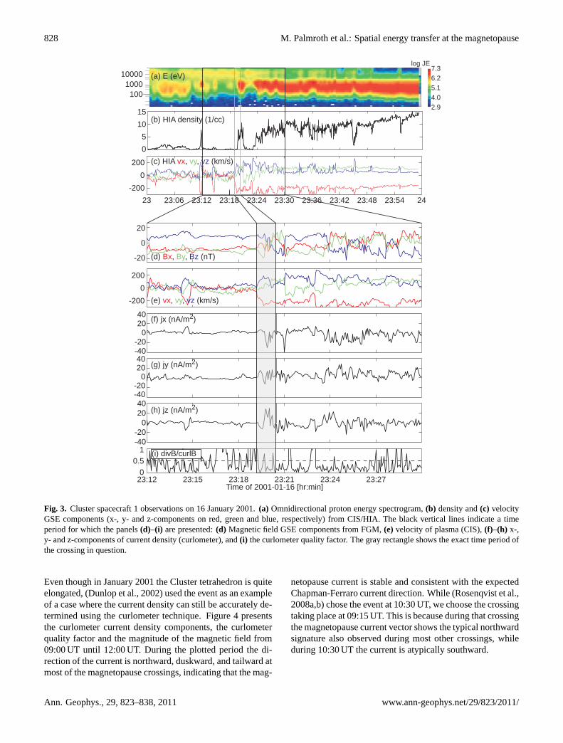
Figure 3 presents the first Cluster (spacecraft 1) magne-topause crossing at [4.4, 9.2, 9.3]RE investigated in thispaper. The panels (a)–(c) of Fig.3 show the overall pic-ture of the time period around the magnetopause crossing,representing the CIS omnidirectional proton energy spectro-gram, the CIS density, and the CIS GSE velocity compo-nents from 23:00 UT until midnight. Just after 23:00 UT,Cluster observed the high energy population of the magne-tosphere, while at the end of the presented period near mid-night the dense magnetosheath low energy population wasobserved. The data show several crossings of the magne-topause, of which some are partial showing mixed popu-lations of magnetosheath-like and magnetospheric plasma(e.g., at 23:23 UT). At 23:19 UT a full crossing occurs, dur-ing which the spacecraft passes from the magnetosphereproper into the magnetosheath proper. After 23:23 UT, theenergy spectrogram shows that the spacecraft encounteredthe magnetopause vicinity several times. During each ofthese encounters, the plasma velocities increased (especiallyin thevz component shown in blue). This indicates a ratherstationary high speed plasma stream near the magnetopause,indicating that the structure of the magnetopause during theplotted period is rather stationary, while the magnetopausedoes move towards and away from the spacecraft quite a bit.

Figure3d–i are blow-ups of the period marked with blacklines in Fig.3a–c, representing 18 min worth of data. Quan-tities needed to determineQ are shown in the plot: themagnetic field (Fig.3d) and plasma velocity components(Fig. 3e), as well as the current density components deter-mined by the curlometer technique (Fig.3f–h). During Jan-uary 2001, the spacecraft separation was sufficiently small toallow accurate determination ofJ , and in Fig.3i we plot theratio of magnetic field divergence over the magnitude of curl.The curlometer gives reliable estimates on the current density

Ann. Geophys., 29, 823–838, 2011 www.ann-geophys.net/29/823/2011/

M. Palmroth et al.: Spatial energy transfer at the magnetopause 827

400

200

0

2

1

0

3

42

6

108

400

350

300

42

6

0

8

240

120

0

360

07:00 08:00 09:00 10:00Time of 2001-01-26

Epsilon (GW)

Dynamic pressure (nPa)

Density (cm-3)

Speed (km/s)

Magnetic field intensity (nT)Mean Bx = -0.8 nT

IMF clock angle (°) Cluster crossing

20:00 21:00 22:00 23:00Time of 2001-01-16

Cluster crossing

Epsilon (GW)

Dynamic pressure (nPa)

Density (cm-3)

Speed (km/s)

Magnetic field intensity (nT)Mean Bx = -2.0 nT

IMF clock angle (°)

(a)

(b)

(c)

(d)

(e)

(f)

(g)

(h)

(i)

(j)

(k)

(l)

11:00

Fig. 2. Four hours worth of Advanced Composition Explorer (ACE) solar wind observations on 16 January 2001 (left panels), and on 26January 2001 (right panels). A delay of 1 h 11 min and 1 h 9 min from ACE position to +15RE has been added, respectively.(a) and(g) IMFclock angle in the yz-plane,(b) and(h) magnetic field intensity,(c)and(i) solar wind speed,(d) and(j) solar wind density,(e)and(k) dynamicpressure, and(f) and(l) ε parameter computed using the solar wind parameters. The vertical lines denote the Cluster magnetopause crossingson each day.

when this ratio is smaller than 0.5 (Dunlop et al., 2002).The period from 23:12 UT until 23:19 UT shows positiveBzcomponent, whileBx is negative, indicating that Cluster wascrossing the dayside magnetopause equatorward of the cusp.The At 23:19 UT, an anti-sunward, duskward and northwardcurrent is observed, and the magnetic field rotates reachingvalues of the magnetosheath magnetic field. The curlometerquality factor in Fig.3g shows that except for a few points,the current estimate is reliable.

Next, we estimate the magnetopause normal and velocityfor the 16 January event. The first block of Table1 shows theresults of the single-spacecraft analysis of the magnetopausenormal, de Hoffman-Teller velocity, and magnetopause ve-locity in the normal direction. The largest ratio of the in-termediate and normal eigenvalues is given by the MVABmethod. The velocity of the magnetopause in the normaldirection is around−20 km s−1 for the methods using mag-netic field records. Since the spacecraft velocity is negligiblecompared to the magnetopause velocity, the magnetopause

moves inward over the spacecraft during this outbound cross-ing; i.e., the velocity direction is opposite to the outwardpointing normal vector, explaining the negative sign in themagnetopause velocity. We also performed the CVA analy-sis for the magnetopause crossing using the magnetic fieldL component in the boundary layer frame (using the MVABnormal from spacecraft 1) from all four spacecraft around the23:19 UT. The results for the multi-spacecraft analysis aregiven in the second block of Table1. The multi-spacecraftanalysis is consistent with the MVAB analysis, suggestingthat the magnetopause velocity during the event is around−30 km s−1. We use both these values in the rest of the pa-per.

3.3 Magnetopause crossing on 26 January 2001

The second interval of interest occurred in the morning of 26January 2001. This interval is extensively studied previouslyas it includes several consecutive magnetopause crossingsover a period of almost three hours (Bosqued et al., 2001).

www.ann-geophys.net/29/823/2011/ Ann. Geophys., 29, 823–838, 2011

828 M. Palmroth et al.: Spatial energy transfer at the magnetopause

15

10

5

0

200

0

-200

20

0

-20

200

0

-200

200

-20

40

-40

200

-20

40

-40

200

-20

40

-401

00.5

23 24

23:12 23:15 23:18 23:21 23:24 23:27Time of 2001-01-16 [hr:min]

23:06 23:12 23:18 23:24 23:30 23:36 23:42 23:48 23:54

(i) divB/curlB

(d) Bx, By, Bz (nT)

(e) vx, vy, vz (km/s)

(f) jx (nA/m2)

(g) jy (nA/m2)

(h) jz (nA/m2)

100001000

100

(a) E (eV)

2.94.05.16.27.3

log JE

(b) HIA density (1/cc)

(c) HIA vx, vy, vz (km/s)

Fig. 3. Cluster spacecraft 1 observations on 16 January 2001.(a) Omnidirectional proton energy spectrogram,(b) density and(c) velocityGSE components (x-, y- and z-components on red, green and blue, respectively) from CIS/HIA. The black vertical lines indicate a timeperiod for which the panels(d)–(i) are presented:(d) Magnetic field GSE components from FGM,(e) velocity of plasma (CIS),(f)–(h) x-,y- and z-components of current density (curlometer), and(i) the curlometer quality factor. The gray rectangle shows the exact time period ofthe crossing in question.

Even though in January 2001 the Cluster tetrahedron is quiteelongated, (Dunlop et al., 2002) used the event as an exampleof a case where the current density can still be accurately de-termined using the curlometer technique. Figure4 presentsthe curlometer current density components, the curlometerquality factor and the magnitude of the magnetic field from09:00 UT until 12:00 UT. During the plotted period the di-rection of the current is northward, duskward, and tailward atmost of the magnetopause crossings, indicating that the mag-

netopause current is stable and consistent with the expectedChapman-Ferraro current direction. While (Rosenqvist et al.,2008a,b) chose the event at 10:30 UT, we choose the crossingtaking place at 09:15 UT. This is because during that crossingthe magnetopause current vector shows the typical northwardsignature also observed during most other crossings, whileduring 10:30 UT the current is atypically southward.

Ann. Geophys., 29, 823–838, 2011 www.ann-geophys.net/29/823/2011/

M. Palmroth et al.: Spatial energy transfer at the magnetopause 829

Table 1. Magnetopause normal and velocity analysis for 16 January 2001; time interval 23:18:48 UT to 23:20:28 UT. Ratio is the ratio ofintermediate and normal eigenvalue given by the analysis,vHT is the de Hoffman Teller velocity, andvHT ·n gives the magnetopause velocityin the normal direction.

Method Ratio vHT Normal vHT ·n (km s−1)

Minimum variance (MVAB) 11.4 (−186.5,−1.6, 116.3) (0.57 0.31 0.76) −17.9Minimum Faraday residue (MFR) 10.2 (−145.1, 84.4, 40.7) (0.55 0.33 0.77) −20.5Minimum mass flux residue (MMR) 4.8 (−228.6, 103.0, 84.3) (0.93 0.09 0.36) −171.8Minimum entropy residue (MER) 4.6 (−229.5, 103.4, 84.3) (0.93 0.09 0.37) −171.6Combined (MVAB, MFR, MMR, MER) 3.4 (−193.4, 59.0, 86.3) (0.74 0.27 0.62) −72.6

Constant velocity analysis (CVA) (0.66 0.32 0.67) −24.1

Fig. 4. The current density inferred using the curlometer technique, from 09:00 UT until 12:00 UT at 26 January 2001. Highlighted in greyare two magnetopause crossing, at 09:15 UT and 10:30 UT.

Figure5a–c present one hour of data on 26 January 2001,from Cluster spacecraft 1 at approximately [3.5 6.7 9.1]RE,in the same format as in Fig.3. According toBosqued etal. (2001), the core magnetosheath population is observedat 09:17 UT (after the second gray vertical line in Fig.5a–c). The transition from the magnetosphere into the coremagnetosheath population occurs through a boundary layer,

where mixed populations of magnetosheath-like and mag-netospheric populations are observed. After 09:14 UT, thespacecraft traverses through the boundary layer into thesheath. The presented period includes many partial crossingsor skimmings of the Earthward edge of the boundary layer,during which high-velocity plasma jets oriented roughly par-allel to the magnetopause are observedBosqued et al.(2001).

www.ann-geophys.net/29/823/2011/ Ann. Geophys., 29, 823–838, 2011

830 M. Palmroth et al.: Spatial energy transfer at the magnetopause

These observations indicate that the jets are associated withthe structure of the boundary layer during the event.

Figure5d–i shows 18 min worth of data around the mag-netopause crossing in the same format as in Fig.3d–i. Theperiod from 09:06 UT until 09:11 UT is associated with al-most zeroBx, and negativeBz, indicating a dayside crossingequatorward of the cusp. At about 09:15 UT, the magneticfield rotates, the velocity components show a distinct change,and the current density shows an anti-sunward, duskwardand northward increase consistent with the Chapman-Ferrarocurrent direction circulating the cusps in the post-noon sec-tor. Notice that during most of the skimmings of the bound-ary layer, such as at 09:23 UT, the current direction is anti-sunward, dawnward, and northward. This current directionis parallel to theB × v electric field, and hence we arguethat the current signature observed during these periods isnot the Chapman-Ferraro system, but is associated with thehigh-velocity jets.

We performed a similar single spacecraft and multi space-craft boundary orientation and velocity analysis as for the 16January case. The results are presented in Table2. As thecrossing does not occur from the magnetosphere proper intothe sheath proper, the quality of the results are not as good asin the 16 January case. The MVAB method yields again thelargest eigenvalue ratio. The CVA timing analysis is difficultas all four spacecraft do not cross the entire magnetopauselayer. However, we performed the timing analysis using thefirst clear magnetosphere-to-boundary layer magnetic struc-ture, and obtained a value of−58 km s−1 for the magne-topause velocity. The value is similar to the one found inBosqued et al.(2001), who obtained−40 km s−1 using bothsingle- and multi-spacecraft methods later during the sameday, at 10:30 UT. As the duration of the 09:15 UT crossing isalso similar to the 10:30 UT crossing, we use in the rest ofthe analysis the value−40 km s−1, agreeing sufficiently wellwith the CVA and MVAB.

4 GUMICS runs

GUMICS-4 was executed with the solar wind input from theperiods given in Fig.2. The smallest grid spacing in thesimulation runs is 0.25RE, ensuring a sharp boundary at themagnetopause. Due to the code setup where the solar windmagnetic field needs to be divergenceless, solar windBx wasset to zero. The dipole tilt angle in both runs is set to zero,otherwise the code setup is typical that has been used in sev-eral event simulations (e.g., Palmroth et al., 2003). There areindications that the IMFBx and the tilt angle affect the re-connection line location (e.g., Trenchi et al., 2008) and hencethe approximations for the tilt angle and the IMFBx mightbe invalid in investigations of the load and generator areas.However, as the negative tilt in January and the negativeIMF Bx shift the reconnection line into opposite directions,and the negative tilt has only a slight effect in the North-

ern Hemisphere where the Cluster crossings occur (Palmrothet al., 2011), the assumptions concerning the tilt and IMFBx are valid. Figure6 illustrates the Cluster orbits on 16January (left panels) and 26 January (right panels) overlaidwith GUMICS-4 reproduction of the plasma density for bothevents.

5 Results: energy transfer and conversion onmagnetopause

Figure7 shows the total energy computations and azimuthalenergy distributions for the 16 January event. The temporalvariation of the total energy transfer through the GUMICS-4 magnetopause resembles that of theε parameter, whilethe magnitudes are different. This is due to the fact thatε

is scaled to the magnetospheric energy consumption, whilethe GUMICS-4 energy transfer (Eq.1) includes all energytransferred through the surface untilx = −30RE, which isnot necessarily deposited within the ionosphere or the innermagnetosphere. Therefore, Fig.7b also shows theε parame-ter scaled with the simulation magnetopause mean area (red)during the run instead of the traditional 4πl20 scaling param-eter, wherel0 = 7RE. The vertical lines in Fig.7b denote thetime instants at which we present azimuthal energy transferdistributions shown in Fig.7c computed using Eq. (2). Theφ

axis at the outer circle shows the magnetopause in yz-planelooking tailward, and the energy transfer through each sector1φ is given by a bar, whose size is proportional to the energyinput in that sector, normalized to the outer circle (100 GW).The black line and dot in each energy distribution shows theIMF orientation and clock angle.

The azimuthal energy transfer distributions in Fig.7cclearly show that during southward IMF, the energy trans-fers through the magnetopause surface in sectors alignedwith the plane of the IMF due to the Poynting flux focussing(Palmroth et al., 2003): the electromagnetic energy vectorpoints towards the magnetopause in those locations, wherethe newly opened field lines are advecting tailwards, becauseonly at those locations the magnetic field lines are at an an-gle with the magnetosheath velocity field allowing a nonzeroPoynting flux. The field line advection in sectors alignedwith the plane of the IMF is also predicted by the Coolingmodel (Cooling et al., 2001) used to track the flux transferevents on the magnetopause. In Fig.7c, it is important tonotice that while the rightmost distribution resembles the en-ergy transfer distribution during the actual Cluster magne-topause crossing, the distributions are all qualitatively sim-ilar: they are all tilted in the plane of the IMF that staysbetween 116◦ and 166◦. Based on Fig.7c, we expect a pri-ori that the energy conversion on the Cluster magnetopausecrossing will be small, as Cluster is not sampling the mag-netopause in the sector of large energy transfer (see Clusterposition in Fig.6b).

Ann. Geophys., 29, 823–838, 2011 www.ann-geophys.net/29/823/2011/

M. Palmroth et al.: Spatial energy transfer at the magnetopause 831

15

10

5

0

2000

-200

20

0

-20

2000

-200

0

50

-50

1

00.5

(i) divB/curlB

(d) Bx, By, Bz (nT)

(e) vx, vy, vz (km/s)

(f) jx (nA/m2)

(g) jy (nA/m2)

(h) jz (nA/m2)

(b) HIA density (1/cc)

(c) HIA vx, vy, vz (km/s)-400

-400

9 1009:06 09:12 09:18 09:24 09:30 09:36 09:42 09:48 09:54

0

50

-50

0

50

-50

09:06 09:12 09:18 09:2409:09 09:15 09:21Time of 2001-01-26 [hr:min]

2.73.95.16.37.5

log JE

100001000100

(a) E (eV)BC A

BC A

Fig. 5. Cluster spacecraft 1 observations on 26 January 2001, from spacecraft 1.(a) Omnidirectional proton energy spectrogram,(b) densityand(c) velocity GSE components (x-, y- and z-components on red, green and blue, respectively) from CIS/HIA. The black vertical linesindicate a time period for which the panels(d)–(i) are presented:(d) magnetic field GSE components from FGM,(e) velocity of plasma(CIS), (f)–(h) x-, y- and z-components of current density (curlometer), and i) the curlometer quality factor. The gray rectangle, verticaldashed lines and letters A, B and C refer to Table3.

Figure 8 shows theε parameter, total energy transfer inGUMICS-4 as well as the azimuthal energy transfer distri-butions for 26 January, in the same format as in Fig.7. Thevertical lines are now showing the time instants separatedby 10 min, and centered by the Cluster magnetopause cross-ing that took place about 09:15 UT. Again, the energy trans-fers in the plane of the IMF, and the distributions in Fig.8cstay qualitatively similar at an after 09:15 UT, although the

amount of the transferred energy varies slightly. The scaledε

is again in good accordance with the simulation energy inputthrough the magnetopause. Figure6d shows the Cluster or-bit for the denoted time instants, and now the spacecraft crossthe magnetopause in a sector, where also a large amount ofenergy is transferring. Hence, we again expect that Clus-ter observes a large amount of energy conversion during themagnetopause crossing.

www.ann-geophys.net/29/823/2011/ Ann. Geophys., 29, 823–838, 2011

832 M. Palmroth et al.: Spatial energy transfer at the magnetopause

Table 2. Magnetopause normal and velocity analysis for 26 January 2001; time interval 09:14:30 UT to 09:15:20 UT. The format is the sameas in Table1.

Method Ratio vHT Normal vHT ·n (km s−1)

Minimum variance (MVAB) 3.3 (−321.6 68.9 145.7) (0.45−0.20 0.87) −33.3Minimum Faraday residue (MFR) 2.4 (−73.9 161.4 41.3) (0.42−0.01 0.91) 5.2Minimum mass flux residue (MMR) 1.0 (−36.1 82.7 25.4) (0.54−0.83 0.16) −83.9Minimum entropy residue (MER) 1.1 (−21.0 87.8 16.1) (0.54−0.82 0.15) −81.4Combined (MVAB, MFR, MMR, MER) 2.5 (−253.4 90.9 116.9) (0.44−0.12 0.89) −19.0

Constant velocity analysis (CVA) (0.60 0.33 0.73) −58.2

Fig. 6. Cluster spacecraft positions (magenta circles) on 16 January(panelsa andb), and 26 January (panelsc andd) during the periodpresented in Fig.2. The colorcoding is the GUMICS-4 reproductionof logarithm of plasma density during the two events. Panels(a) and(c) are depicted in xy-plane atz = 0, whereas panels(b) and(d) arethose for yz-plane atx = 0.

Figure9 shows the results of the detailed comparison be-tween the GUMICS-4 simulation against the Cluster esti-mate of the energy conversion, calculated using the data fromtimes highlighted with gray in Figs.3 and5. The left (right)panels are again for 16 January (26 January) events. The toprow shows the GUMICS-4 energy conversion computed us-ing Eq. (3), while the second row gives the energy transferusing Eq. (1). The magnetopause is viewed from the frontlooking tailwards. The magenta dots give the Cluster posi-tion in each event at the given time. The GUMICS-4 resultson the energy conversion and transfer at the Cluster posi-tion are given in the respective legends of Fig.9a–b and9d–e. The GUMICS-4 results for 16 January are evaluated at23:15 UT, and 09:15 UT on 26 January. The energy transferdistributions depicted in Fig.9b and9e are almost as muchtilted with respect of due south and show almost similar mag-nitudes of energy transfer as the other solar wind conditions

0

100

200

300

400

500(a) Epsilon (GW)

2001−01−16

21 22 23 240

500

1000

1500

2000(b) GUMICS total energy input (GW) Epsilon scaled with GUMICS m’pause area (GW)

50 100

30

210

60

240

90270

120

300

150

330

180

0

θ = 116o

(c) Az. energy distributions (GW)

50 100

30

210

60

240

90270

120

300

150

330

180

0

θ = 136o

50 100

30

210

60

240

90270

120

300

150

330

180

0

θ = 151o

50 100

30

210

60

240

90270

120

300

150

330

180

0

θ = 161o

50 100

30

210

60

240

90270

120

300

150

330

180

0

θ = 166o

Fig. 7. (a)Theε parameter for 16 January event, delayed to +15REusing a delay 1 h 11 min.(b) Total energy transfer through themagnetopause in the GUMICS-4 simulation against time in the 16January event (black) andε parameter scaled with the simulationmagnetopause area (red). Vertical lines denote the times at whichthe instantaneous energy transfer distributions in(c) are given. Thesize of the bar in panels(c) gives the portion of energy transfer inthe yz-plane integrated from the nose to−30RE. The bar size isnormalized to the outer circe (100 GW), and the IMF orientationis given by the black line, with the filled dot referring to the clockangle given in the bottom left legend of each distribution.

are similar. The bottom row gives the Cluster estimate of theenergy conversionQ using Eq. (5) in the two events. Theintegral of the energy conversion through the magnetopauseis computed as a cumulative sum, and hence the final valueof the plotted curve given in the legend of Fig.9c, f is to becompared with the simulation results. The Cluster estimatefor 16 January is computed using two values for the mag-netopause velocity: 20 km s−1 (black) and 30 km s−1 (red),while the value for 26 January uses 40 km s−1 found hereand inBosqued et al.(2001).

Figure9 illustrates that on 16 January, the spatial distri-bution of energy conversion and transfer is tilted away from

Ann. Geophys., 29, 823–838, 2011 www.ann-geophys.net/29/823/2011/

M. Palmroth et al.: Spatial energy transfer at the magnetopause 833

Table 3. Cluster estimations of the energy conversion using different time intervals and including all current density values in the calculation(Q1) and omitting those current density values where the curlometer quality factor is larger than 0.5 (Q2). The difference (%) tells howmuchQ1 differs fromQ2.

Time Q1 (µW m−2) Q2 (µW m−2) vmp (km s−1) Difference

16 January 2001

23:18:36–23:20:27 UT −8.6 −5.3 20 38 %23:18:36–23:20:27 UT −12.8 −8.0 30 38 %

26 January 2001

A: 09:14:27–09:16:23 −106.4 −95.9 40 10 %B: 09:13:30–09:16:23 −102.1 −89.1 40 13 %C: 09:11:31–09:16:23 −130.0 −114.3 40 12 %

0

100

200

300

400

500(a) Epsilon (GW)

2001−01−26

8 9 10 110

500

1000

1500

2000

2500

(b) GUMICS total energy input (GW)Epsilon scaled with GUMICS m’pause area

50 100

30

210

60

240

90270

120

300

150

330

180

0

θ = 183o

(c) Az. energy distributions (GW)

50 100

30

210

60

240

90270

120

300

150

330

180

0

θ = 213o

50 100

30

210

60

240

90270

120

300

150

330

180

0

θ = 224o

50 100

30

210

60

240

90270

120

300

150

330

180

0

θ = 230o

50 100

30

210

60

240

90270

120

300

150

330

180

0

θ = 234o

Fig. 8. (a)Theε parameter for 26 January event, delayed to +15REusing a delay 1 h 9 min.(b) Total energy transfer through the mag-netopause in the GUMICS-4 simulation against time in the 26 Jan-uary event (black) andε parameter scaled with the simulation mag-netopause area (red). Vertical lines denote the times at which theinstantaneous energy transfer distributions in(c) are given. The for-mat of the figure is the same as Fig.7.

the north-south direction, and occurs in the northern dawnand southern dusk sectors at the magnetopause. The Clustercrossing of the magnetopause occurs in between the load andgenerator regions away from the strongest energy conversionand transfer, and indeed in Fig.9c the Cluster estimate ofthe energy conversion within the magnetopause current layeris small, only from−8 to −13 µW m−2. The Cluster esti-mate is larger than in GUMICS, but still in quantitative ac-cordance with the simulation results: The simulation showslittle energy conversion and transfer, as the conversion esti-mate is about−3 µW m−2 and transfer about−4 µW m−2.The pixels neighboring the Cluster crossing location givesimilar magnitudes, but can be of different sign. On 26 Jan-

uary, however, Cluster crosses the magnetopause in a regionwhere the simulation results indicate large energy conversionand transfer. Based on the simulation, the location of thecrossing occurs well within the generator region as now theneighboring pixels show similar magnitudes and sign for en-ergy conversion, indicating also that our initial assumptionsof the tilt angle and IMFBx are valid. The simulation esti-mates for the conversion and transfer are−28 µW m−2 and−50 µW m−2, respectively, lower than the Cluster estimate,which is−106 µW m−2. In both events, the Cluster estimateof the energy conversion exceeds that of the GUMICS-4 lo-cal energy conversion by the same factor∼4.

Table3 gives Cluster estimations of the energy conversionfrom the two events using different crossing parameters. The16 January crossing is “clean”, such that there is no ambigu-ity on the timing of the crossing, and as indicated by Fig.3,the spacecraft traverses from the magnetospheric-like intosheath-like population rapidly without observing a boundarylayer. The ambiguity within the crossing comes from the ex-act value of the magnetopause velocity, and the few pointsof possibly erroneous curlometer current density measure-ments. Hence, we present theQ calculation using the twomagnetopause velocity values as well as omitting the datapoints having a larger curlometer quality factor than 0.5. ThevalueQ1 is hence computed using all points from the timeperiod, but in computing the valueQ2 the points where thecurlometer quality factor exceeds the 0.5 limit are set to zero.As the GUMICS-4 result was−2.9 µW m−2, the Cluster es-timate is larger by a factor of 2–3.

The 26 January event is more ambiguous in timing, asthe spacecraft flies through the boundary layer and the high-velocity jets and their associated currents disturb the timingbased on the current density increase. Table3 shows the dif-ferences in estimates forQ in three crossing durations (let-ters A, B, and C in Fig.5). Taking into account the ambiguityassociated with the timing, the curlometer, and the velocityof the magnetopause, our best estimate of the energy con-version within the magnetopause in the 26 January event is

www.ann-geophys.net/29/823/2011/ Ann. Geophys., 29, 823–838, 2011

834 M. Palmroth et al.: Spatial energy transfer at the magnetopause

−30

−20

−10

0

10

20

302001−01−16: 23:15 UT

(a) Pec

at Cluster: −2.9 μW/m2

Simulation energy conversion

ZG

SE [R

E]

−40 −20 0 20 40−30

−20

−10

0

10

20

30

YGSE

[RE]

(b) Pmp

at Cluster: −4.2μW/m2

Simulation energy transfer

ZG

SE [R

E]

18:54 19:12 19:30 19:48 20:06−15

−10

−5

0

5x 10

−5

Time after 23 UT [min:sec]

cum

sum

(Q)

[W/m

2 ]

c) Cluster observationsQ (v

mp = 20 km/s): −8.5

Q (vmp

= 30 km/s): −12.8

2001−01−26: 09:15 UT

(d) Pec

at Cluster: −28.3μW/m2

Simulation energy conversion

−25

0

25

50

μW/m2

−40 −20 0 20 40Y

GSE [R

E]

(e) Pmp

at Cluster: −50.3μW/m2

Simulation energy transfer

−25

0

25

50

15:00 15:36 16:12−15

−10

−5

0

5x 10

−5

Time after 09 UT [min:sec]

Q (vmp

= 40 km/s): −106.0(f) Cluster observations

Fig. 9. Left (right) panels: results for 16 January at 23:15 UT (26 January at 09:15 UT).(a) and(d) divergence of the Poynting vector at themagnetopause surface in the GUMICS-4, looking tailwards from the front of the magnetopause.(b) and(e) total energy transfer through themagnetopause surface in the GUMICS-4.(c) and(f) Cumulative sum (representing the time evolution of theQ integral) of energy conversionat Cluster orbit through the magnetopause; red (black) curve usingvmp= 20 (30) km s−1 for 16 January. The magenta dots in panels(a), (b),(d) and(e)show the Cluster position on the given time, and the values in the respective legends show the simulation result on Cluster positionat the given time. The Cluster estimate of the integral of the energy conversion (the final value of the cumulative sum) in the magnetopausecurrent layer is given in the legends of panels(c) and(f). All values in legends are given in µW m−2

about−100 µW m−2, again larger by a factor of 3 comparedto the GUMICS-4 local values. Hence in both events, am-biguity of the measurements explained a factor of 1 discrep-ancy between the measurements and the simulation results,but the same scaling factor of 2–3 was found between theCluster observations and the simulation results.

6 Discussion

In this paper, our main goal is to use the simulation to verifythe IMF By dependence of the spatial energy transfer sug-gested by earlier simulations (Palmroth et al., 2003). We canalso take the opportunity to estimate the global energy trans-fer using the two local measurements to scale the simulation

Ann. Geophys., 29, 823–838, 2011 www.ann-geophys.net/29/823/2011/

M. Palmroth et al.: Spatial energy transfer at the magnetopause 835

results. We find the same scaling parameter (a factor of 2–3)from both local estimates. We have also briefly reviewed themethodology developed earlier to infer the simulation energytransfer and conversion from GUMICS-4 global MHD simu-lation (Palmroth et al., 2003; Laitinen et al., 2006, 2007). Thetwo methods represent two complementary viewpoints in themagnetopause energetics and they are both consequences ofthe dayside magnetopause reconnection. The energy trans-fer method tells us how much total energy (kinetic, electro-magnetic and thermal) transfers across the magnetopause,while the energy conversion method yields an estimate ofhow much of the transferring energy is converted from oneform to another, and directly evaluates the power consumedby reconnection. Hence in principle, the magnitude of en-ergy conversion cannot exceed that of the energy transfer.The spatial variation of the transfer and conversion is notnecessarily exactly the same as the integrals are different,although using primarily the same quantities. The energyconversion occurs primarily within or adjacent to the recon-nection region, but energy can transfer (via Poynting flux fo-cussing) anywhere on the surface, where open field lines ex-ist. The energy conversion method should be comparable tothe Cluster methodology (Rosenqvist et al., 2006) in a time-independent case, as shown by Eq. (4). Time-independencyis a good assumption if the magnetopause structure remainssteady during the event. This is the case in both of the eventsdiscussed here.

In computing the Cluster estimate of the magnetopause en-ergy conversion, obvious sources of errors include the deter-mination of the current density and the magnetopause veloc-ity. Especially the latter is a constant multiplier in Eq. (5) andorder-of-magnitude errors would introduce an order of mag-nitude discrepancy in the final estimation. Here, we havecarefully measured the velocity of the magnetopause. Wehave also used the best available method (curlometer) to in-fer the current density, and we note that the single space-craft methods yield similar values (not shown). Hence, ourcurrent density estimate is generally reliable, while instan-taneous observations include uncertainties that lead to dis-crepancies within the final estimate (Table3). As witnessedduring the 26 January 2001 event, the magnetopause can in-clude local effects that are associated with boundary layerdynamics. Hence, we argue that the timing should be done ascarefully as possible, so that only the large scale Chapman-Ferraro current contributes toQ. Special care should be paidon the timing of the event if it includes spiky current densityfeatures that are not consistent with the large-scale currentdirection. However, one of the most important finding of thispaper is that even with the best possible means to infer energyconversion (multi-spacecraft techniques, carefully selectedevents and stable upstream conditions) an uncertainty factorexists within the observations. Here, the final estimates in-clude 10 %–40 % differences, which were due to timing, ve-locity of the magnetopause as well as momentary bad valuesof the curlometer. We envisage that in more dynamic events

having unstable upstream conditions, the discrepancies canbe larger.

The 26 January case was also one of many crossings anal-ysed byRosenqvist et al.(2008b,a). They +67 µW m−2 forQ at 10:30 UT and interpreted the event as being a cross-ing of the load region. Using the BATS-R-US global MHDsimulation,Rosenqvist et al.(2008a) computed bothQ and−∇ ·S from the simulation results along the Cluster orbit.The comparison yielded favorable results only after they ar-tificially lowered the spacecraft trajectory in the simulationtowards the subsolar magnetopause. We note that inRosen-qvist et al.(2008a,b) the a priori assumption on the load na-ture of the crossing was made based on the current theoreti-cal understanding that the load exists equatorward of the cusp(Lundin and Evans, 1985). However, most importantly, thecurrent density during the 10:30 UT event shows southwardsignatures, while typically the magnetopause crossings on 26January show northward current densities (Fig.4). Flippingthe sign of theJz to positive at 10:30 UT flips the sign ofQinto negative, consistent with our findings of the 09:15 UTcrossing. Since the current shows northward signatures dur-ing several of the crossings, we note that the current densitydirection at 09:15 UT is consistent with the global Chapman-Ferraro direction, while the 10:30 UT crossing possibly in-cludes local signatures that influence the current direction.The global simulations cannot easily reproduce local signa-tures, while the global pattern is reproduced on average. In-deed, Fig.9 shows a large positive region equatorward ofthe generator region, and hence the artificial lowering of thespacecraft orbit in a simulation would yield a good agree-ment.

The current theoretical understanding states that the loadregion resides equatorward of the cusp, while the genera-tor region is found poleward of the cusp. The Cluster re-sults shown in this paper suggest that generator region canbe found from the dayside magnetosphere on field lines thatare equatorward of the cusp. The use of the spatially limitedcusp to distinguish the load and generator regions is mislead-ing especially for nonzero IMF y when the magnetosphericaxis of symmetry is not in the noon-midnight meridian. Forinstance in the presented 26 January 2001 case, the IMF yis negative and hence the cusps are found from the north-ern pre-noon and the southern post-noon regions (Newell etal., 1989), while the Cluster crossing occurs in the northernpost-noon, a large longitudinal distance away from the cusp.Instead, we argue that theoretically the accurate separator forthe load and generator regions, at least for low-latitude recon-nection, is the location at which the solar wind thrust forceexceeds theJ ×B stress caused by the curvature of the openfield line. In other words, the separator for load and gen-erator should appear where the Alfven velocity equals themagnetosheath velocity, and the field line is being draggedby the magnetosheath flow instead of being accelerated byreconnection. As such, this occurs tailward of the last closedfield line that indeed is the cusp field line somewhere on the

www.ann-geophys.net/29/823/2011/ Ann. Geophys., 29, 823–838, 2011

836 M. Palmroth et al.: Spatial energy transfer at the magnetopause

surface, and hence the cusp is a special case of this generalcondition. While it would be interesting to find this separator,we leave it for further study with a notion that the separatorsearch should start by finding a location where the accelera-tion fields caused by the magnetosheath flow and theJ ×B

force are in balance. This also introduces interesting avenuesfor further studies of the magnetopause energy transfer as itsuggests that the load and generator regions (their sizes andpossibly also their intensities) can be dependent on the mag-netosheath velocity field, which in turn is related not only tothe velocity of the solar wind but also to the shock structure.

In a global simulation using a quantitative methodologythe a priori assumptions are more easily formed as the out-come of the calculation is plainly visible as in Fig.1, em-phasizing the power of the approach combining the simu-lations with observations. When looking at the simulationdata giving a full three-dimensional global picture of the twoevents, the Cluster estimates fall naturally in place and arealmost in quantitative agreement with the simulation results.We believe that here the Cluster estimate and the simula-tion results validate each other: the simulations show thatthe large differences in the Cluster estimates is natural anddue to the spatial variation of energy transfer and conversion.On the other hand, the carefully measured Cluster estimatepins down the magnitudes of the simulation results. Assum-ing that the comparison between in situ observations and thesimulation is as good also in other parts of the magnetopause,we are able to pin down the total energy transfer during thetwo time instants. We estimate that the total energy transfer-ring through the magnetopause during the two events is about1500–2000 GW, three times the value ofε. Theε representsPoynting flux through a circular area of radiusl0, where theradius is used to scale the energy input to equal the magneto-spheric output. To make the simulation results more directlycomparable withε, we have scaled theε again with the mag-netopause mean area during the events, as measured from thesimulation. Our results show that the local values in the sim-ulation are underestimated by a factor of probably 2–3, whilethe scaledε is in quantitative agreement with the simulationenergy input. This indicates thatε is underestimated basedon the evidence of this paper. In accordance,Koskinen andTanskanen(2001) also suggested in a broad review of theε

parameter thatε should be scaled up by a factor of 1.5–2.

7 Summary and conclusions

We conclude that the GUMICS-4 simulation results are ingood agreement with the Cluster observations in these twocases. The magnitude of energy conversion in the simula-tion, obtained by means that are directly comparable to themethodology using the Cluster observations, is around 30 %of the Cluster estimate during both events, without any as-sumptions made on the magnetopause velocity or the rela-tive location of the Cluster magnetopause crossing within the

code. The simulation energy transfer values are around 50 %of the Cluster estimate. However, as the observations also in-clude uncertainties, we conclude that using the present gridresolution and within the global framework the comparisonis as perfect as it can be.

Our main findings in this paper are the following:

1. Cluster observations verify the simulation results on theIMF By dependence of the energy transfer on the mag-netopause.

2. To estimate global energy transfer, one should only takecurrent layers being part of the Chapman-Ferraro sys-tem.

3. The separator for load and generator should appearwhere the Alfven velocity equals the magnetosheath ve-locity, and the field line is being dragged by the magne-tosheath flow instead of being accelerated by reconnec-tion.

4. The amount of energy conversion and transfer inGUMICS-4 agrees well with Cluster observations dur-ing the presented events, even though shows probablya factor of 2–3 lower values, however, also the Clusterestimate ofQ includes ambiguities.

5. The combined results from the simulation and Clusterobservations suggest that theε parameter is underesti-mated by a factor of 2–3.

Acknowledgements.The Cluster data have been retrieved from theCluster Active Archive (CAA), and we thank Harri Laakso andteam for maintaining the system. ACE spacecraft recordings are re-trieved from the ACE homepage (http://www.srl.caltech.edu/ACE/).We thank the ACE MAG and SWEPAM PI’s C. W. Smith andD. J. McComas for distributing the Level 2 data freely in the in-ternet. We thank the CDAWeb facility for distributing the data. Theresearch leading to these results has received funding from the Eu-ropean Research Council under the European Community’s Sev-enth Framework Programme (FP7/2007-2013)/ERC Starting Grantagreement number 200141-QuESpace. The work of MP is sup-ported by the Academy of Finland. MWD is partly supported byChinese Academy of Sciences (CAS) visiting Professorship for se-nior international scientists grant no. 2009S1-54 and the SpecializedResearch Fund for State Key Laboratories of the CAS.

Guest Editor M. Taylor thanks M. Liemohn and A. R. Retinofor their help in evaluating this paper.

References

Akasofu, S.-I.: Energy coupling between the solar wind and themagnetosphere, Space Sci. Rev., 28, 121–190, 1981.

Axford, W. I. and Hines, C. O.: A unifying theory of high-latitudegeophysical phenomena and geomagnetic storms, Can. J. Phys.39, 1433–1464, 1961.

Balogh, A., Carr, C. M., Acuna, M. H., Dunlop, M. W., Beek, T.J., Brown, P., Fornacon, K.-H., Georgescu, E., Glassmeier, K.-H., Harris, J., Musmann, G., Oddy, T., and Schwingenschuh, K.:

Ann. Geophys., 29, 823–838, 2011 www.ann-geophys.net/29/823/2011/

M. Palmroth et al.: Spatial energy transfer at the magnetopause 837

The Cluster Magnetic Field Investigation: overview of in-flightperformance and initial results, Ann. Geophys., 19, 1207–1217,doi:10.5194/angeo-19-1207-2001, 2001.

Bosqued, J. M., Phan, T. D., Dandouras, I., Escoubet, C. P.,Reme, H., Balogh, A., Dunlop, M. W., Alcayde, D., Amata, E.,Bavassano-Cattaneo, M.-B., Bruno, R., Carlson, C., DiLellis, A.M., Eliasson, L., Formisano, V., Kistler, L. M., Klecker, B., Ko-rth, A., Kucharek, H., Lundin, R., McCarthy, M., McFadden, J.P., Mobius, E., Parks, G. K., and Sauvaud, J.-A.: Cluster observa-tions of the high-latitude magnetopause and cusp: initial resultsfrom the CIS ion instruments, Ann. Geophys., 19, 1545–1566,doi:10.5194/angeo-19-1545-2001, 2001.

Boyle, C. B., Reiff, P. H., and Hairston, M. R.: Empiricalpolar cap potentials, J. Geophys. Res., 102(A1), 111–125,doi:10.1029/96JA01742, 1997.

Cooling, B. M. A., Owen, C. J., and Schwartz, S. J.: Role ofthe magnetosheath flow in determining the motion of open fluxtubes, J. Geophys. Res., 106, 18764–18775, 2001.

Dungey, J. W.: Interplanetary field and the auroral zones, Phys. Res.Lett., 6, 47–48, 1961.

Dunlop, M. W. and Woodward, T. I.: Multi-spacecraft discontinuityanalysis: orientation and motion, in: Analysis methods for multi-spacecraft data, chapter 11, 271–306, edited by: Paschmann, G.and Daly, P. W., ISSI scientific report SR-001, ESA PublicationsDivision, The Netherlands, 1998.

Dunlop, M. W., Balogh, A., Glassmeier, K.-H., and Robert,P.: Four-point Cluster application of magnetic field analysistools: The Curlometer, J. Geophys. Res., 107(A11), 1384,doi:10.1029/2001JA005088, 2002.

Janhunen, P.: GUMICS-3: A global ionosphere-magnetospherecoupling simulation with high ionospheric resolution, in: Pro-ceedings of Environmental Modelling for Space-Based Applica-tions, 18–20 September 1996, Eur. Space Agency Spec. Publ.,ESA SP-392, 1996.

Koskinen, H. E. J. and Tanskanen, E. I.: Magnetospheric energybudget and the epsilon parameter, J. Geophys. Res., 107(A11),1415,doi:10.1029/2002JA009283, 2002.

Laitinen, T. V., Janhunen, P., Pulkkinen, T. I., Palmroth, M., andKoskinen, H. E. J.: On the characterization of magnetic recon-nection in global MHD simulations, Ann. Geophys., 24, 3059–3069,doi:10.5194/angeo-24-3059-2006, 2006.

Laitinen, T. V., Palmroth, M., Pulkkinen, T. I., Janhunen, P.,and Koskinen, H. E. J.: Continuous reconnection line andpressure-dependent energy conversion on the magnetopausein a global MHD model, J. Geophys. Res., 112, A11201,doi:10.1029/2007JA012352, 2007.

Lundin, R. and Evans, D. S.: Boundary layer plasmas as a source forhigh-latitude, early afternoon, auroral arcs, Planet. Space Sci.,33, 1389–1406, 1985.

McComas, D. J., Bame, S. J., Barker, P., Feldman, W. C., Phillips,J. L., Riley, P., and Griffee, J. W.: Solar Wind Electron ProtonAlpha Monitor (SWEPAM) for the Advanced Composition Ex-plorer, Space Sci. Rev., 86, 563–612, 1998.

Newell, P. T., Meng, C.-I., and Sibeck, D. G.: Some low-altitudecusp dependencies on the interplanetary magnetic field, J. Geo-phys. Res., 94, 8921–8927, 1987.

Newell, P. T., Sotirelis, T., Liou, K., Meng, C.-I., and Rich, F. J.: Anearly universal solar wind-magnetosphere coupling function in-ferred from 10 magnetospheric state variables, J. Geophys. Res.,

112, A01206,doi:10.1029/2006JA012015, 2007.Palmroth, M., Pulkkinen, T. I., Janhunen, P., and Wu, C.-C.: Storm-

time energy transfer in global MHD simulation, J. Geophys.Res., 108(A1), 1048,doi:10.1029/2002JA009446, 2003.

Palmroth, M., Laitinen, T. V., and Pulkkinen, T. I.: Magnetopauseenergy and mass transfer: results from a global MHD simu-lation, Ann. Geophys., 24, 3467–3480,doi:10.5194/angeo-24-3467-2006, 2006.

Palmroth, M., Koskinen, H. E. J., Pulkkinen, T. I., Toivanen, P.K., Janhunen, P., Milan, S. E., and Lester, M., Magnetosphericfeedback in solar wind energy transfer, J. Geophys. Res., 115,A00I10,doi:10.1029/2010JA015746, 2010.

Palmroth, M., Fear, R., and Laitinen, T. V.: Magnetopause energytransfer dependence on dipole tilt and solar wind parameters: Aview from a global MHD simulation, in preparation, 2011.

Papadopoulos, K., Goodrich, C., Wiltberger, M., Lopez, R., andLyon, J. G.: The physics of substorms as revealed by the ISTP,Phys. Chem. Earth, 24, 189–202, 1999.

Raeder, J.: Global Magnetohydrodynamics – A Tutorial, in: SpacePlasma Simulation, edited by: Buechner, J., Dum, C. T., andScholer, M., Lecture Notes in Physics, vol. 615, Springer Verlag,Heidelberg, 2003.

Reme, H., Aoustin, C., Bosqued, J. M., Dandouras, I., Lavraud,B., Sauvaud, J. A., Barthe, A., Bouyssou, J., Camus, Th., Coeur-Joly, O., Cros, A., Cuvilo, J., Ducay, F., Garbarowitz, Y., Medale,J. L., Penou, E., Perrier, H., Romefort, D., Rouzaud, J., Vallat, C.,Alcayde, D., Jacquey, C., Mazelle, C., d’Uston, C., Mobius, E.,Kistler, L. M., Crocker, K., Granoff, M., Mouikis, C., Popecki,M., Vosbury, M., Klecker, B., Hovestadt, D., Kucharek, H.,Kuenneth, E., Paschmann, G., Scholer, M., Sckopke, N., Seiden-schwang, E., Carlson, C. W., Curtis, D. W., Ingraham, C., Lin, R.P., McFadden, J. P., Parks, G. K., Phan, T., Formisano, V., Amata,E., Bavassano-Cattaneo, M. B., Baldetti, P., Bruno, R., Chion-chio, G., Di Lellis, A., Marcucci, M. F., Pallocchia, G., Korth,A., Daly, P. W., Graeve, B., Rosenbauer, H., Vasyliunas, V., Mc-Carthy, M., Wilber, M., Eliasson, L., Lundin, R., Olsen, S., Shel-ley, E. G., Fuselier, S., Ghielmetti, A. G., Lennartsson, W., Es-coubet, C. P., Balsiger, H., Friedel, R., Cao, J.-B., Kovrazhkin, R.A., Papamastorakis, I., Pellat, R., Scudder, J., and Sonnerup, B.:First multispacecraft ion measurements in and near the Earth’smagnetosphere with the identical Cluster ion spectrometry (CIS)experiment, Ann. Geophys., 19, 1303–1354,doi:10.5194/angeo-19-1303-2001, 2001.

Rosenqvist, L., Buchert, S., Opgenoorth, H., Vaivads, A., and Lu,G.: Magnetospheric energy budget during huge geomagnetic ac-tivity using Cluster and ground-based data, J. Geophys. Res.,111, A10211,doi:10.1029/2006JA011608, 2006.

Rosenqvist, L., Opgenoorth, H. J., Rastaetter, L., Vaivads, A., andDandouras, I.: Comparison of local energy conversion estimatesfrom Cluster with global MHD simulations, Geophys. Res., Lett.,35, L21104,doi:10.1029/2008GL035854, 2008a.

Rosenqvist, L., Vaivads, A., Retino, A., Phan, T., Opgenoorth,H. J., Dandouras, I., and Buchert, S.: Modulated reconnec-tion rate and energy conversion at the magnetopause understeady IMF conditions, Geophys. Res., Lett., 35, L08104,doi:10.1029/2007GL032868, 2008b.

Shue, J.-H., Chao, J. K., Fu, H. C., Russell, C. T., Song, P., Khurana,K. K., and Singer, H. J.: A new functional form to study the solarwind control of the magnetopause size and shape, J. Geophys.

www.ann-geophys.net/29/823/2011/ Ann. Geophys., 29, 823–838, 2011

838 M. Palmroth et al.: Spatial energy transfer at the magnetopause

Res., 102(A5), 9497–9511,doi:10.1029/97JA00196, 1997.Shue, J.-H., Song, P., Russell, C. T., Steinberg, J. T., Chao, J.

K., Zastenker, G., Vaisberg, O. L., Kokubun, S., Singer, H. J.,Detman, T. R., and Kawano, H.: Magnetopause location underextreme solar wind conditions, J. Geophys. Res., 103, 17691–17700, 1998.

Shukhtina, M. A., Gordeev, E. I., and Sergeev, V. A.: Time-varying magnetotail magnetic flux calculation: a test of themethod, Ann. Geophys., 27, 1583–1591,doi:10.5194/angeo-27-1583-2009, 2009.

Siscoe, G. L. and Cummings, W. D.: On the cause of geomagneticbays, Planet. Space Sci., 17, 1795–1802, 1969.

Smith, C. W., Acuna, M. H., Burlaga, L. F., Heureux, J. L., Ness,N. F., and Scheifele, J.: The ACE magnetic fields experiment,Space Sci. Rev., 86, 613–632, 1998.

Sonnerup, B. U.O., Haaland, S., Paschmann, G., Dunlop, M.W., Reme, H., and Balogh, A.: Orientation and motion ofa plasma discontinuity from single-spacecraft measurements:Generic residue analysis of Cluster data, J. Geophys. Res., 111,A05203,doi:10.1029/2005JA011538, 2006.

Trenchi, L., Marcucci, M. F., Pallocchia, G., Consolini, G., Bavas-sano Cattaneo, M. B., Di Lellis, A. M., Reme, H., Kistler, L.,Carr, C. M., and Cao, J. B., Occurrence of reconnection jets atthe dayside magnetopause: Double Star observations, J. Geo-phys. Res., 113, A07S10,doi:10.1029/2007JA012774, 2008.

Ann. Geophys., 29, 823–838, 2011 www.ann-geophys.net/29/823/2011/