Research Division Federal Reserve Bank of St. Louis Working Paper Series

Spatial Dependence in Models of State Fiscal Policy Convergence

Cletus C. Coughlin Thomas A. Garrett

and Rubén Hernández-Murillo

Working Paper 2006-001B http://research.stlouisfed.org/wp/2006/2006-001.pdf

January 2006 Revised June 2006

FEDERAL RESERVE BANK OF ST. LOUIS Research Division

P.O. Box 442 St. Louis, MO 63166

______________________________________________________________________________________

The views expressed are those of the individual authors and do not necessarily reflect official positions of the Federal Reserve Bank of St. Louis, the Federal Reserve System, or the Board of Governors.

Federal Reserve Bank of St. Louis Working Papers are preliminary materials circulated to stimulate discussion and critical comment. References in publications to Federal Reserve Bank of St. Louis Working Papers (other than an acknowledgment that the writer has had access to unpublished material) should be cleared with the author or authors.

Spatial Dependence in Models of State Fiscal Policy Convergence*

Cletus C. Coughlin Thomas A. Garrett

Ruben Hernandez-Murillo

Federal Reserve Bank of St. Louis

Draft Date: June 23, 2006

Abstract

We apply spatial econometric techniques to models of state and local fiscal policy convergence. Total tax revenue and expenditures, as well as broad tax and expenditure categories, of state and local governments in each of the 48 contiguous U.S. states are examined. We extend work by Scully (1991) and Annala (2003) in much the same way that Rey and Montouri (1999) extended the literature dealing with income convergence among U.S. states. Our results indicate that most fiscal policies have been converging and exhibit spatial dependence. A more specific interpretation of our general spatial results is that the finding of spatial dependence indicates that the growth paths of state and local fiscal policies are not independent. In addition, we find that total expenditures have been converging faster than output, whereas total tax revenues have been converging slower that output. Our models further demonstrate that state expenditure growth is dependent upon expenditure growth in economically and demographically similar states, while output growth and revenue growth in a state are dependent on output growth and revenue growth, respectively, in contiguous states.

JEL Codes: C21, H71, H72, R11 Keywords: convergence, state fiscal policy, fiscal policy dependence, spatial econometrics * The views expressed here are those of the authors and are not necessarily the views of the Federal Reserve Bank of St. Louis or the Federal Reserve System.

2

Spatial Dependence in Models of State Fiscal Policy Convergence

Introduction

Neoclassical growth models as developed by Solow (1956) predict that incomes

across space (e.g. countries or states) will converge over time.1 For such convergence to

occur, lower income jurisdictions must experience higher growth rates than higher

income jurisdictions. Convergence as a process of long-run growth has received

significant attention in the academic literature. Beginning with Easterlin (1960),

�������� ����� ������ ���� �������� ����� �� �-convergence or divergence across

countries (Pritchett, 1997; Hoover and Perez, 2004), Canadian provinces (DeJuan and

Tomljanovich, 2005), U.S. states (Barro and Sala-i-Martin, 1995; Carlino and Mills,

1996; Webber et al., 2005), U.S. counties (Bukenya et al., 2002), and geographic regions

(Miller and Gene, 2005).2 In the United States, state incomes have generally been

converging over time, although a temporary divergence was seen in the 1970s and 1980s

(Coughlin and Mandelbaum, 1988; Carlino and Mills, 1996). Although estimated speeds

of convergence depend upon the units of observation and the sample period, studies of

U.S. states suggest a speed of convergence of roughly two percent a year (Barro and

Sala-i-Martin, 1995).

One potential problem with many of the preceding studies stems from an

underlying assumption that each cross-sectional unit is independent. However, as

discussed in Rey and Montouri (1999) and Abreu et al. (2004), units of observation, such 1 By contrast, endogenous growth models as developed by Romer (1986) allow for divergence. 2� ��� � �-convergence test for income convergence is done by regressing average annual income growth on an initial level of income. A negative value for the estimated coefficient on initial income indicates convergence while a positive value indicates divergence. Another form of convergence, σ−convergence, refers to a decline in the standard deviation of income over time. Work by Fingleton (2003), Magrini (2004) and Rey and Janikas (2005) provide surveys of the convergence literature and critiques of the various empirical methodologies used.

3

as states or countries, are typically defined by politically established boundaries rather

than economic boundaries. Technology spillovers, migration, trade flows, commuting

patterns and public policy can link economies together despite their political separation.

Ignoring the possible spatial interactions between economic units in an empirical model

may lead to incorrect inferences regarding the magnitude and significance of economic

variables (Anselin, 1988; Rey and Janikas, 2005).

Numerous studies, such as Moreno and Trehan (1997), Conley and Ligon (2002),

Ramirez and Loboguerrero (2002), and Le Gallo (2004), have applied spatial

econometric techniques to traditional models of income convergence and have found

strong evidence that the income growth of a country is dependent upon the income

growth of neighboring countries. Even more relevant to the current study is the work of

Rey and Montouri (1999), who have generated new insights concerning the geographical

features of state income growth and on the role of geography in the econometric analysis

of state income convergence. We extend recent work by Scully (1991) and Annala

(2003) on fiscal policy convergence in much the same way that Rey and Montouri (1999)

extended the literature dealing with income convergence among U.S. states.

The study of converging state and local government fiscal policies is a

straightforward extension of traditional income convergence studies. The growth model

by Solow (1956) implies that the growth rates of tax revenue and government

expenditures are equal to the growth rate of income under the assumption that taxes are a

constant proportion of output.3 Based on the Solow growth model and the finding of

3 In reality, taxes and expenditures are not a constant portion of income. However, there is relatively little variability over time. For example, U.S. Federal government revenues have averaged 18.5 percent of GDP between 1977 and 2002, with a standard deviation of 0.95 percent. At the state and local level, revenues to

4

state income convergence by previous studies, it is a reasonable hypothesis that state

fiscal policies are also converging.

Based on a public-choice model, Scully (1991) has examined this hypothesis. In

contrast to a Tiebout (1956) model in which migration reinforces the differences in local

fiscal regimes, migration contributes to the convergence of fiscal regimes in Scully’s

model. The theory is straightforward, beginning with the idea that migration contributes

to a convergence of incomes across regions. Assuming that voter preferences for net

public income transfers do not differ across regions, fiscal regimes will converge

spatially as incomes converge. Empirically, Scully finds that the spatial convergence of

total state and local taxes coincides with the spatial convergence of per capita incomes

across states.

Recently, Annala (2003) has extended the empirical portion of Scully’s (1991)

analysis by examining the convergence of several state and local fiscal policy variables

(revenue sources and expenditure categories) over the period 1977 to 1996. He finds

strong support for state fiscal policy convergence – most expenditure and revenue

categories grew at a greater rate in those states having a lower initial level of expenditure

and revenue. For example, Annala (2003) finds that the growth rate in total state and

local tax revenue and expenditures have been converging at roughly 4.8 percent and 4.0

percent a year, respectively.

In this paper we extend the work of Scully (1991) and Annala (2003) by

considering spatial dependence in models of state and local fiscal policy convergence.

Our spatial econometric models follow those used by Rey and Montouri (1999) in their

state and local governments have averaged 9.6 percent of gross domestic product between 1977 and 2002, with a standard deviation of 0.5 percent.

5

study of state income convergence. Because spatial dependence has been found in

traditional models of income growth, it is reasonable to believe that growth in state and

local fiscal policy is also correlated across states. Citizen preference for taxation and

government services, while certainly different at an individual level, are not dependent

upon the location of a state or local government boundary. This notion is empirically

supported by Case et al. (1993) who find evidence that the level of per capita government

expenditures in a state is positively related to the level of government expenditures in

neighboring states. In addition, unobserved regional shocks to government revenues and

expenditures suggest spatial correlation in the error structure of convergence models.

Applying spatial econometrics to models of state fiscal policy convergence can

offer new insights into the behavior of long run fiscal policy growth. First, the presence

of spatial dependence suggests that earlier estimates of rates of state fiscal policy

convergence may be biased unless spatial effects are incorporated into the analysis. In

addition to reducing bias, a greater efficiency of coefficient estimates can be obtained if

spatial correlation is considered (Anselin, 1988). Second, the potential for spatial

dependence in long run state fiscal policy growth will provide evidence on how these

fiscal policies interact over time. In particular, evidence of spatial dependence suggests

that states’ fiscal policies are not converging independently of each other’s but rather

display similar paths because of strategic interaction or common responses to regional

shocks. From this we can gain insights that contribute to the literature on tax competition

and intergovernmental competition in general (Kanbur and Keen, 1993; Besley and Case,

1995; Wilson, 1991, 1999; Hernandez-Murillo, 2003; Bailey et al., 2004).4

4 In a recent survey Brueckner (2003) illustrates the use of spatial econometrics models to analyze strategic interaction among different governmental units.

6

Data and Empirical Methodology

We use data for each of the 48 contiguous states for 1977 and 2002.5 Gross state

product and the nine fiscal policy variables enumerated in Table 1 are in real per capita

dollars and encompass both state and local governments unless specified otherwise.6 All

state and local government tax and expenditure data were obtained from the U.S. Bureau

of the Census, Federal, State, and Local Government Division. Gross state product data

were obtained from the Bureau of Economic Analysis.

[Table 1 about here]

Preliminary evidence on converging or diverging state and local fiscal policies

can be generated by computing the coefficient of variation for each fiscal policy variable

for the initial year and the ending year. The coefficient of variation reflects dispersion

from the mean and can be used to compare the degree of inequality for each fiscal policy

variable in the two years, with each year having a different mean.7 A smaller coefficient

of variation in 2002 compared to 1977 suggests a converging policy, whereas a larger

coefficient of variation in 2002 suggests a diverging policy.

The computed coefficients of variation, shown in Table 2, reveal that total tax

revenues and expenditures as well as most broad categories of taxes and expenditures

have been converging over the sample period. For example, the coefficient of variation

5 Annala (2003) used data on all 50 states for 1977 and 1996. We ignore Alaska and Hawaii because they have very unique economies. States with no state sales tax (Alaska, Delaware, Oregon, New Hampshire, and Montana) are excluded from the analysis of sales tax convergence (n=44). The states with no state personal income tax (Florida, Nevada, South Dakota, Texas, Washington and Wyoming) are omitted from the analysis of income tax convergence (n=42). The results were similar when New Hampshire and Tennessee (state personal income tax on dividend and interest only) were omitted from the analysis. 6 Real gross state product is in chained 2000 dollars, while all fiscal policy variables have been deflated using the consumer price index, whose base is 1982-1984=100. 7 The coefficient of variation for gross state product and each fiscal policy variable is computed as:

2 0.5

1

[{ ( ) / 47} ]/N

ii

CV FP FP FP=

= −∑ where FP denotes the fiscal policy variable as well as, to simplify the

notation, gross state product.

7

for total tax revenues declined from 0.22 in 1977 to 0.18 in 2002, while the coefficient of

variation for total expenditures declined from 0.18 in 1977 to 0.14 in 2002. With respect

to broad categories of taxes and expenditures, public welfare expenditures and income

tax revenue (for those states having state income taxes) have become less diverse across

states over time, followed by education expenditures and highway expenditures. The

coefficient of variation for sales tax and gross receipts revenue (for those states having a

state sales tax) is virtually identical for 1977 and 2002. Only health and hospital

expenditures appear to be diverging over the sample period.8 Finally, the coefficient of

variation of gross state product has declined only slightly, thus suggesting little

convergence between 1977 and 2002.

[Table 2 about here]

Empirical Methodology

Although the coefficients of variation provide initial insights into the convergence

of state and local fiscal policies over time, traditional regression methods are better suited

to obtaining estimates on the speed of convergence as well as incorporating spatial

dependence. Our empirical methodology is presented below.

For each state, we calculate the average annual percent change (YFP) in gross state

product and each fiscal policy variable (FP) as:

YFP = [ln(FP/pop)2002 – ln(FP/pop)1977]/T

8 Our results differ from Merriman and Skidmore (2002), who found that the coefficient of variation in per capita state government health care spending declined between 1988 and 1998. We found an increase in the coefficient of variation between 1988 and 1998. The difference appears to be due to what is included in health care spending. Following Annala (2003), we use the hospitals and health categories of social services and income maintenance spending, while Merriman and Skidmore (2002) have also included medical vendor payments. A second difference is that Merriman and Skidmore (2002) use state government expenditures, while we also include local government expenditures.

8

where T is the number of time periods and pop is state population. We then use this

variable as the dependent variable in the following ���� �� �-convergence:

(1)

where the (unconditional) speed of convergence or divergence for each fiscal policy

variable is determined by the sign and magnitude of �1.9

As discussed in the introduction, the existence of spatial dependence can create

bias and efficiency problems for estimates of �1 based on a standard ordinary least

squares regression. The general spatial econometric model (Anselin, 1988) allows for

potential spatial correlation in both the dependent variable (fiscal policy growth in this

case) and the error term. The spatial econometric model does not induce cross-sectional

correlation if none is present; it simply provides an established and flexible framework

for relaxing the assumption of cross-sectional correlation with regard to a model's

dependent variable and/or error term. As Anselin (1988) notes, unlike time-series

correlation that is one dimensional, spatial correlation in cross-sectional models is multi-

dimensional in that it depends upon all contiguous or influential units of observations (in

this case states). Incorporating spatial effects into the convergence model presented

earlier gives the following spatial econometric model, specified in matrix notation:

9 The st������� ���� �� �-convergence has been criticized for several reasons. Quah (1993) notes that implicit in the empirical specification is the idea that each economy has a steady-state growth path that follows a time trend. He provides cross-county evidence on income growth that refutes this assumption. Durlauf (2001) points to several problems inherent in traditional convergence models, such as the potential for spillover effects and nonlinearities, a disconnect between growth theory and empirical modeling (i.e., which variables should be included in growth models and how the potential problem of simultaneity between these variables should be handled), and, finally, heterogeneous parameters (i.e., the marginal change in a variable may produce different effects in very different countries). We recognize the potential ������� � �� �� ���� ��� � � �������� ���� �� �-convergence, but we argue that differences across states in terms of heterogeneous parameters and different growth paths is likely to be significantly less than across countries due to the fact that political systems and components of government revenue and spending are much more similar across states than across countries. In addition, we account for spillover effects in our empirical model, thereby addressing a concern of Durlauf (2001).

0 1 1977FPY FPβ β ε= + +

9

0 1 1977FP FPβ β ρ= + + +Y FP WY ε (2a)

λ= +ε ε νW (2b)

The spatial lag component is given by �WYFP, where W denotes the exogenous

(N×N) spatial weights matrix. The scalar ρ is the spatial lag, or spatial autoregressive,

coefficient that must be estimated. Positive spatial correlation in fiscal policy growth

exists if ρ > 0, negative spatial correlation exists if ρ < 0, and no spatial correlation exists

if ρ = 0.10 The spatial error component of the model is given by λ= +Wε ε ν , where � is

a (N×1) vector of error terms, W is the same (N×N) spatial weights matrix as in equation

(2a), ν is a (N×1) white noise error component, and � � ��� ���� ����� ��������� ����

must be estimated.

The errors are positively correlated if � �� ������� � ����� ���� � � �� ���� �

������� ���� � � ��� Spatial error correlation can result from omitted variables,

including spatially weighted independent variables and a spatial lag, and unobserved

spatial heterogeneity in the error structure (Anselin, 1988). Note that if there is no spatial

correlation in the dependent variable or the error structure, then ρ � � � ��� ��� ������ �

spatial model reduces to the standard ordinary least squares regression model. Typically,

spatial lag and spatial error models are estimated separately to avoid possible

identification problems (Anselin, 1988). In models of strategic interaction among

governments, the spatial lag parameter is usually interpreted as the slope of the reaction

function. Brueckner (2003) indicated that strategic interaction may correspond to several

interpretations of the underlying game among governments, including models of tax

10 Generally, when a spatial weights matrix is row-standardized, the values for the spatial correlation coefficients are smaller than 1 and larger than the inverse of the smallest eigenvalue of the weights matrix. See Anselin (1995).

10

competition and yardstick competition. Spatial correlation in the error term, on the other

hand, can be interpreted as reflecting states’ common reaction to shocks because of

omitted variables that are spatially correlated, such as topographical features.11

Since the spatial lag term in Equation (2a) is correlated with the error term and the

spatial error component is also non-spherical, estimating equations (2a) and (2b) by

ordinary least squares will result in biased, inconsistent, and inefficient parameter

estimates (Anselin, 1988). Assuming the random component of the spatial error (ν ) is

homoskedastic and jointly normally distributed, Equations (2a) and (2b) can be estimated

by maximum likelihood.12,13

The elements of the spatial weights matrix (W) are generally specified a priori.

The elements of W commonly reflect a measure of contiguity or distance between units

of observation. The most common weights matrix in the growth literature (and the

applied spatial econometrics literature in general) is the binary contiguity matrix (Cliff

and Ord, 1981; Anselin, 1988). In this representation, the individual elements of W,

denoted �ij, are set equal to unity if observations i and j (i� j) share a common border,

and are set to zero otherwise. The limitations of this specification are that all neighboring

observations are assumed to have equal influence and any spatial correlations beyond

common-border neighbors are ignored.

11 In the models surveyed by Brueckener (2003), the spatial lag model is used to estimate reaction functions in strategic games of tax or yardstick competition among governments. Ignoring spatial correlation in the error term in this case may provide false evidence of strategic interaction. 12 See Anselin (1988) for a description of the likelihood function for the spatial lag and spatial error models. We use programs in James P. LeSage’s Econometrics Toolbox to run the spatial models. The programs can be found at: www.spatial-econometrics.com. 13 As an alternative to maximum likelihood, Kelejian and Prucha (1998) suggest a method based on instrumental variables that yields a consistent estimate of ρ even in the presence of spatial error dependence. This method traditionally uses the independent variables and their spatial lags as instruments. We chose not use this method in our final estimations because, in our case, the sole independent variable corresponding to the initial values of the fiscal policies turned out to be a poor instrument for the spatial lag of the growth rate.

11

It is not clear, however, that geography is the most relevant factor in capturing

spatial dependence in long run fiscal policy growth. States may formulate their fiscal

policies based not only on the behavior of their neighbors, but also on the policies of

states sharing similar economic or demographic characteristics regardless of their

proximity. Although choosing weights matrices is somewhat arbitrary (Case et al, 1993),

we have chosen three weights matrices that are likely to best capture spatial correlation in

state policy decisions.14 We therefore follow Case et al. (1993) and specify three

different weights matrices, one based on proximity (border) and economics (income), and

two based on proximity (border) and demographics (percent of population that is black or

percent of population aged 65 years or older). Our three weights matrices are:

Wincome � �WI + (1-��WG

Wrace � �WR + (1-��WG

Wage � �WA + (1-��WG

Each element of WG is equal to one divided by the number of borders state i shares if

states i and j share a common border. Individual elements of WI are equal to 1/|incomei –

incomej|���j1/|incomei – incomej|) where incomei is real per capita income in state i.

Elements of WR equal 1/|blacki – blackj| ���j1/|blacki – blackj|), where blacki is the

proportion of state i’s population that is black, and the elements of WA are equal to

1/|agedi – agedj| ���j1/|agedi – agedj|), where agedi is the proportion of state i’s population

that is aged 65 years or older.15 The elements along the diagonal of each weights matrix

(i=j) are set to zero by convention. T�� �� �� �� � is determined by a grid-search of log-

likelihoods (0 � � � 1). Each weights matrix collapses to the standard contiguity matrix

14� ������ � ����� �������� � ����� � ���������� � ��� � ��� � ����������� � �� �� � 15 We use the 1976 value for incomei, blacki , and agedi . Using 1977 values would render each weights matrix endogenous.

12

(WG) � ��� . A finding of � �1 suggests that economics or demographics defines a

spatial neighbor better than contiguity.

Empirical Results

For gross state product and each of the fiscal policy variables, we estimate one

ordinary least squares model and three spatial autoregressive (SAR) and spatial error

(SEM) models using each of the spatial weights matrices described earlier.16 Our

regression results are shown in Table 3.17

[Table 3 about here]

Evidence of Fiscal Policy Convergence

The results support several general conclusions regarding state and local fiscal

policy convergence, most of which are consistent with Annala (2003).18 The regression

results present strong evidence that state and local fiscal policies have been converging.

Our estimated speeds of convergence are less, however, than those obtained by Annala

(2003). In addition to our inclusion of spatial effects, this is likely due to the fact that our

sample period extends to 2002, which includes the recent 2001 recession. As shown in

Owyang et al. (2005), both the timing and the magnitude of the 2001 recession were not

homogenous across the states – many states entered their own recession prior to the

official National Bureau of Economic Research start date for the U.S. recession (March

16 We also estimated a model that included the spatially-weighted fiscal policy variable, i.e. WFP1977, to capture the possibility that long run fiscal policy growth in a state is a function of the initial level of fiscal policy in neighboring states. The coefficient on this variable was not statistically significant for any of the nine fiscal policies, thus we chose to omit this variable from our final models. 17 The results shown in Table 3 are the log-likelihood maximizing results from a grid search of all possible ������ � �� � � �� ��� ���� ������� � ��� � ���� � �� ���� ���������� ������ � �� � �������� ��� � � � � � � � � ����� � ��������� ��provided a large amount of output, which will gladly be provided upon request. 18 We also estimated our models using the 1977 to 1996 sample period of Annala (2003). The spatial econometric results using this shorter sampler period are very similar to those presented here, and the conclusions regarding fiscal policy convergence are generally consistent with those of Annala (2003).

13

2001) and exited the recession after the official ending date (November 2001). This was

especially true for the traditionally poorer states of the south. Thus, extended periods of

negative income growth, revenue growth, and expenditure growth, especially in poorer

states, can explain a greater divergence (or less convergence) in these later years.

Regardless of the regression model, the results indicate that seven of the nine

variables we study are converging over the sample period. For two fiscal policy

variables, sales taxes and gross receipts and health and hospital expenditures, the

evidence for convergence is, at best, weak. For these variables the estimate of �1 is

always negative, but statistically significant relationships are found only for the

autoregressive models for sales taxes and gross receipts and are not found for any of the

models using health and hospital expenditures. Annala (2003) obtains similar results for

sales taxes and health expenditures over the period 1977 and 1996. Like Annala (2003),

we find that none of the fiscal policy variables have been diverging over the sample

period.

For the seven fiscal policies that have been converging, the speed of convergence

is similar across all seven regression models, although the speed of convergence is often

slightly less, on average, when spatial effects are considered. For example, if we

consider total tax revenue, the ordinary least squares model suggests a speed of

convergence of about 1.3 percent a year, whereas the average annual speed of

convergence of the spatial models ranges from 1.0 percent to 1.2 percent.

Comparing the average speed of convergence based on the spatial models for the

broad categories of fiscal policies, it appears that public welfare expenditures have had

the greatest speed of convergence – roughly 2.6 percent a year. Highway and education

14

expenditures round out the top three fastest converging fiscal policies, each having had

average speeds of convergence of 1.8 percent. The fiscal policy with the lowest

statistically significant average speeds of convergence is property tax revenue (roughly

0.7 percent a year).19

Finally, it is interesting to compare the speed of convergence of gross state

product (a measure of output) and several government fiscal policy variables. We find

that, on average, gross state product has been converging at a rate of roughly 1.2 percent

a year. In comparison, total expenditures have had a speed of convergence of about 1.5

percent a year and total tax revenue has had a speed of convergence of about 1.1 percent

a year. These statistics reveal that total expenditures have been converging faster than

output and that total tax revenues have been converging slightly slower than output. This

broadly suggests that state governments, especially those with lower initial levels of

general expenditures, have been increasing expenditures faster than the average rate of

economic growth. It also appears that the driving force behind this rate of growth is

public welfare expenditure that, of all government expenditure variables, has had the

greatest speed of convergence.

Evidence of Fiscal Policy Dependence

While the literature on intergovernmental competition mainly focuses on spatial

dependence in short-run state or local government policies that arise out of action-

reaction type responses by competing governments, our models better demonstrate the

long-run effect of interstate competition. The first result is that in six of the nine cases

19 Although property taxes are predominately a decision of local governments, state governments often legislate restrictions and other laws on local property taxes, such as assessment rates, revenue caps, etc.

15

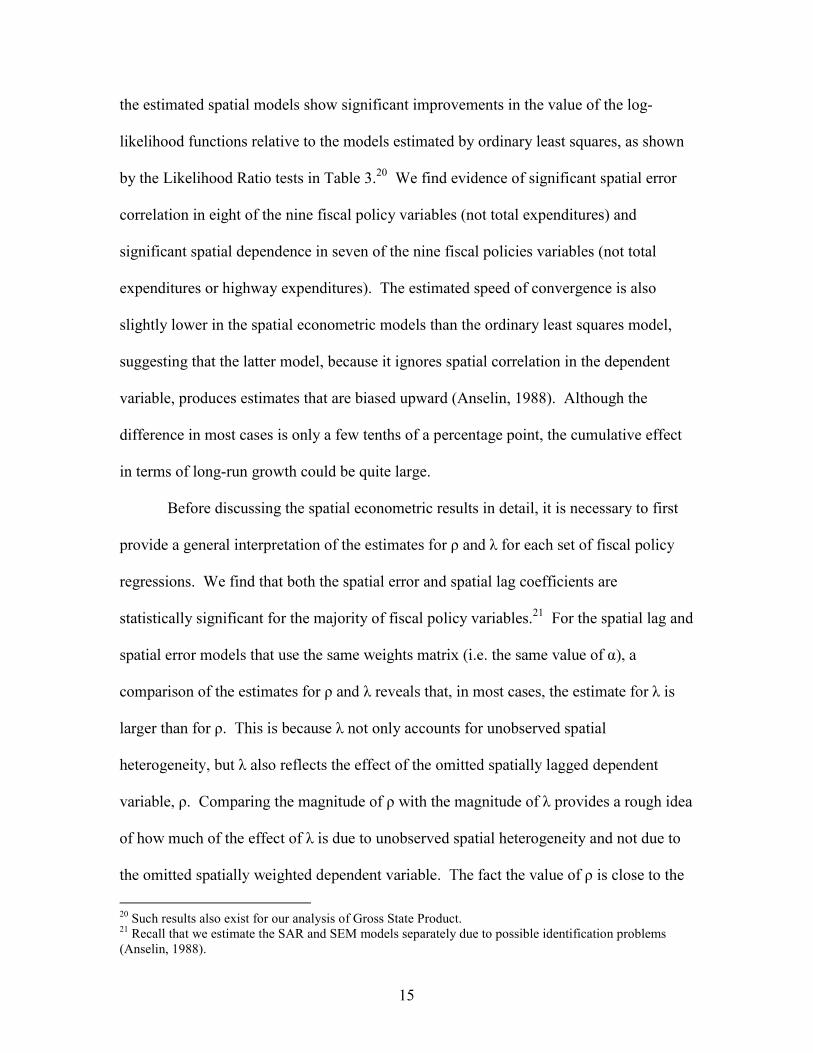
the estimated spatial models show significant improvements in the value of the log-

likelihood functions relative to the models estimated by ordinary least squares, as shown

by the Likelihood Ratio tests in Table 3.20 We find evidence of significant spatial error

correlation in eight of the nine fiscal policy variables (not total expenditures) and

significant spatial dependence in seven of the nine fiscal policies variables (not total

expenditures or highway expenditures). The estimated speed of convergence is also

slightly lower in the spatial econometric models than the ordinary least squares model,

suggesting that the latter model, because it ignores spatial correlation in the dependent

variable, produces estimates that are biased upward (Anselin, 1988). Although the

difference in most cases is only a few tenths of a percentage point, the cumulative effect

in terms of long-run growth could be quite large.

Before discussing the spatial econometric results in detail, it is necessary to first

����� � ������ ����������� �� ��� �������� ��� ��� ��� ���� ��� �� ���� � �� �

regressions. We find that both the spatial error and spatial lag coefficients are

statistically significant for the majority of fiscal policy variables.21 For the spatial lag and

���� ����� ���� � ���� ��� ��� ���� ������ ���� ���� ��� ���� �� �� �� �� ��

�������� �� ��� �������� ��� ��� ����� � ����� � ���� ������ ��� ������� ��� � � �

����� ���� ��� � !�� � "������ ��� � only accounts for unobserved spatial

������������� "�� � �� ��� ���� ��� ������ �� ��� ������ ���� � ����� ���������

����" �� � #������ ��� �������� �� ��� ��� �������� �� ������ � ����� ��� �

�� ��� ���� �� ��� ������ �� � ��� ��� unobserved spatial heterogeneity and not due to

��� ������ ���� � ������� �������� ����" �� !�� ���� ��� �� �� �� is close to the

20 Such results also exist for our analysis of Gross State Product. 21 Recall that we estimate the SAR and SEM models separately due to possible identification problems (Anselin, 1988).

16

value of ��� ��� ��$���� �� ���� ��� �� ���� � �� ���������� �������� ���� ��� "� %�

of the spatial error effect is due to the omitted spatially weighted dependent variable.

Although the spatial error estimates relative to the spatial lag estimates suggest

some degree of spatial error correlation, which may be masquerading as strategic

interaction, it was not possible to disentangle the source of the spatial effects using

diagnostic tests as in Anselin et al. (1996).22 A more specific interpretation of our

general spatial results is that the finding of spatial dependence indicates that the growth

paths of state and local fiscal policies are not independent. To illustrate the effects on

long run policy growth, the remaining discussion of the empirical results will focus on

the SAR models.

&���� �� ��� ������� �� � � e find that a one percentage point average increase

in neighboring states’ gross state product growth will increase a state’s average annual

gross state product growth by 0.37 percentage points. Similarly, a one percentage point

average increase in neighboring states’ total tax revenue growth will increase a state’s

average annual tax revenue growth by roughly 0.38 percent. Finally, a one percentage

point average increase in neighboring states’ total expenditure growth does not appear to

have a statistically significant effect on a state’s average total expenditure growth.

Again, our results do not reveal the direct effects of action-reaction types of policy

competition across states, but rather they demonstrate the long-run effect of such

competition.

The results also provide insights into the broad categories of fiscal policies that

are the most correlated in a spatial sense across states and those that are not correlated

across states. One general finding is that spatial correlation is much more prevalent for 22 Also see footnote #13.

17

revenue categories than for expenditure categories. In fact, we find spatial error

correlation and spatial dependence using all three weights matrices when we use total tax

revenue. In contrast, we find no statistically significant spatial correlation for total

expenditures.

Turning to separate categories, property tax revenue has the greatest degree of

correlation across states – a one percentage point average increase in neighboring states’

property tax revenue growth will increase a state’s property tax revenue growth by 0.56

percent. One explanation for this finding is that property values are similar within

geographic regions but differ across regions (Baffoe-Bonnie, 1998). This fact, coupled

with the trend in the devolution of government services and the fact that property tax

revenue is the primary revenue source for local governments across the country (Fisher,

1996), can explain the relatively large degree of spatial dependence in property tax

revenue. It is also interesting to note that while property tax revenues have the greatest

degree of spatial dependence across states, the speed at which they are converging is the

slowest (about 0.7 percent a year) of all fiscal policy variables having a statistically

significant �1. This finding likely reflects the growing dispersion in home values across

different regions of the country (e.g., Midwest versus the east and west coasts).23

We find little evidence that health and hospital expenditures are spatially

correlated. Health expenditures are likely to be based on the health needs of each state’s

population. It is more difficult for a state to change its health expenditures when its

population and its health needs are relatively constant one year to the next. States may

thus find it more difficult to spend more on health than is needed by its population.

23 See the house price index, by Census region, produced by the Office of Federal Housing and Oversight (http://www.ofheo.gov/HPIRegion.asp).

18

Several interesting conclusions can also be made regarding the spatial weights

matrix that best captures (in terms of maximizing the log-likelihood) the nature of spatial

dependence in each fiscal policy variable. An especially interesting result is that

contiguity is, by far, the key factor in capturing the spatial dependence in the revenue

variables. In the vast majority of cases for the revenue variables we find th�� ��� �����

suggests that contiguity is the exclusive factor in the construction of the weights matrix.

For the expenditure variables, however, income, race, and age are useful in capturing the

spatial correlation. Proximity continues to play a role, but to a lesser degree than it did

for the revenue variables. This suggests that economic growth (measured by gross state

product) and the revenue streams based on economic growth (e.g. income tax revenue,

sales tax revenue, etc.) are a function of economic growth in neighboring states,

regardless of whether these states share similar economic and demographic

characteristics.

For the majority of expenditure variables, with education expenditures being the

exception, we find that economic and/or demographic similarities across the states play a

role in capturing the spatial correlation. The proximity of the states to one another still

matters in many cases, but certainly not to the extent it matters for the revenue variables.

For example, the spatial dependence of public welfare expenditures depends relatively

more on income and demographics than on proximity. On the other hand, proximity

matters more than income and demographics in terms of capturing spatial dependence in

education expenditures across states.

In sum, there is strong evidence that expenditure growth in a state is dependent

upon the expenditure growth in economically and demographically similar states,

19

regardless of the states’ location to each other. Economic growth and tax revenue growth

in a state, however, appear to be most dependent upon the economic growth and tax

revenue growth in contiguous states regardless of their specific economic and

demographic similarities.

Summary and Conclusions

We have contributed to the empirical literature on fiscal policy convergence by

extending the traditional convergence model to allow for spatial correlation across states.

Specifically, we apply the spatial econometric techniques used in studies of income

growth to a model of long run state and local fiscal policy growth. Of the nine fiscal

policies examined in this study, we find strong evidence that seven of the nine have been

converging over the period 1977 to 2002. Speeds of convergence range from about 0.7

percent a year for property tax revenue to 2.6 percent a year for public welfare

expenditures. We also find that total tax revenues have been converging slightly slower

than output and that total government expenditures have been converging faster than

output. This latter point suggests that poorer states have been increasing government

expenditures faster than the average rate of economic growth.

While our results are supportive of previous results on state and local fiscal policy

convergence, we do find that our estimates are somewhat smaller in magnitude. Two

explanations for this finding are: 1) the time period our analysis covers includes the 2001

recession where economic growth and government revenues and expenditures slowed

considerably, yet unequally across the states, and 2) the inclusion of spatial dependence

in the model reduces the potential for bias.

20

We find strong evidence that long run state and local fiscal policy growth in one

state is a function of long run of fiscal policy growth in neighboring states. For example,

we find that a one percentage point average increase in neighboring states’ total tax

revenue growth will increase a state’s average annual tax revenue growth by roughly 0.38

percent. Of all the fiscal policies we studied, property tax revenue growth exhibits the

greatest degree of spatial dependence, with a spatial lag coefficient of 0.56. We argue

this finding reflects the increasing nationwide role local governments have taken relative

to state governments in providing goods and services.

Our analysis also considered several different source of spatial influence –

geography, economics, and demographics. Many of the spatial lag and spatial error

coefficients in each set of fiscal policy models are statistically significant regardless of

which weighting scheme is used. However, we find that the spatial effects for state

revenue policies are generally different than for expenditure policies. Specifically,

expenditure growth in a state is dependent upon the expenditure growth in economically

and demographically similar states, regardless of the states’ locations to one another.

However, output growth and revenue growth in a state appears to be most dependent on

the output growth and revenue growth in contiguous states regardless of their specific

economic and demographic similarities. This likely reflects the notion that states who

share a common border are more likely to have economies and revenue streams that are

similarly affected by changes in economic conditions, whereas state expenditures, the

bulk of which is education and public welfare, are more a function of the income and

demographic characteristics of each state.

21

Future research could explore the possibility of spatial clusters (Rey and Janikas,

2005). One approach to doing so is that the spatial econometric models could be

modified to allow the spatial lag and spatial error coefficients to differ by geographic

region, thus providing insights into how long run fiscal policy growth may differ by

region. Similarly, it would be of interest to explore whether the degree of spatial

dependence in fiscal policy growth changes over time. This may have relevance for the

political business cycle literature. Finally, there is an opportunity for future research to

better identify differences in both speeds of convergence and spatial dependence during

recessionary periods versus periods of economic growth.

22

References

Abreu, M., De Groot, H., Florax, R.(2004) Space and growth: A survey of empirical evidence and methods. Tinbergen Institute Discussion Paper no. 04-129/3. Annala, C. (2003) Have state and local fiscal policies become more alike? Evidence of beta convergence among fiscal policy variables. Public Finance Review, 31: 144-165. Anselin, L. (1988) Spatial econometrics: Methods and models. Kluwer: Dordrecht. Anselin, L. (1995) SpaceStat, A software program for the analysis of spatial data, Version 1.80. Regional Research Institute, West Virginia University, Morgantown, West Virginia. Anselin, L., Bera A.K., Florax, R., Yoon M.J. (1996) Simple diagnostic tests for spatial dependence. Regional Science and Urban Economics, 26:77-104. Baffoe-Bonnie, J. (1998) The dynamic impact of macroeconomic aggregates on housing prices and stock of houses: A national and regional analysis. Journal of Real Estate Finance and Economics, 17: 179-97. Bailey, M., Rom, T., Taylor, M. (2004) State competition in higher education: A race to the top, or a race to the bottom? Economics of Governance, 5: 53-75. Barro, R., Sala-i-Martin, X. (1995) Economic growth. Advanced Series in Economics. New York: McGraw Hill. Besley, T., Case, A. (1995) Incumbent behavior: Vote-seeking, tax setting, and yardstick competition. American Economic Review, 85: 25-45. Brueckner, J. K. (2003) Strategic interaction among governments: An overview of empirical studies. International Regional Science Review, 26: 175-188. Bukenya, J., Gebremedhin, T., Schaeffer, P. (2002) Income convergence: A case study of West Virginia counties. Research Paper 2002-03, Alabama A&M University. Carlino, G., Mills, L. (1996) Convergence and the U.S. states: A time-series analysis. Journal of Regional Science, 36: 597-616 Case, A., Rosen, H., Hines, J. (1993) Budget spillovers and fiscal policy interdependence: Evidence from the states. Journal of Public Economics, 52: 285-307. Cliff, A., Ord, J. (1981) Spatial processes, models, and applications. Pion, London. Conley, T., Ligon, E. (2002) Economic distance and cross-county spillovers. Journal of Economic Growth, 7: 157-187.

23

Coughlin C., Mandelbaum, T. (1988) Why have state per capita incomes diverged recently? Federal Reserve Bank of St. Louis Review, 70: 24-36. DeJuan, J., Tomljanovich, M. (2005) Income convergence across Canadian provinces in the 20th century: Almost but not quite there. The Annals of Regional Science, 39: 567-592. Durlauf, S. (2001) Manifesto for a growth econometrics. Journal of Econometrics, 100: 65-69. Easterlin, R. (1960) Regional growth of income. In: Kuznets S., Miller A., Easterlin R. (eds.) Population redistribution and economic growth in the United States, 1870-1950. American Philosophical Society, Philadelphia. Fingleton, B. (2003) European regional growth. New York: Springer-Verlag. Fisher, R. (1996). State and local public finance. Irwin: Chicago. Hernandez-Murillo, R. (2003) Strategic interaction in tax policies among states. Federal Reserve Bank of St. Louis Review, 85: 47-56. Hoover, K., Perez, S. (2004) Truth and robustness in cross-country growth regressions. Oxford Bulletin of Economics and Statistics, 66: 765-798. Kanbur, R., Keen, M. (1993) Jeux sans frontieres: Tax competition and tax coordination when countries differ in size. American Economic Review, 83: 877-892. Kelejian, H.H., Prucha, I.R. (1998) A generalized spatial two-stage least squares procedure for estimating a spatial autoregressive model with autoregressive disturbances. Journal of Real Estate Finance and Economics, 17: 99-121. LeGallo, J. (2004) Space-time analysis of GDP disparities among European regions: A Markov chains approach. International Regional Science Review, 27: 138-163. Magrini, S. (2004) Regional (di)convergence. In V. Henderson and J. Thisse (eds) Handbook of regional and urban economics. New York: Elsevier. Merriman, D., Skidmore, M. (2002) Convergence in state government health care spending and fiscal distress. Proceedings: Ninety-fourth Annual Conference on Taxation, Baltimore, MD, November 8-10, 2001 and minutes of the annual meeting of the National Tax Association, 81-89. Miller, J., Gene, I. (2005) Alternative regional specifications and convergence of U.S. regional growth rates. The Annals of Regional Science, 39: 241-252.

24

Moreno, R., Trehan, B. (1997) Location and the growth of nations. Journal of Economic Growth, 2: 399-418. Owyang, M., Piger, J., Wall, H. (2005) Business cycle phases in U.S. states. Review of Economics and Statistics, 87: 604-616. Pritchett, L. (1997) Divergence, big time. Journal of Economic Perspectives, 11: 3-17. Quah, D. (1993) Empirical cross-section dynamics in economic growth. European Economic Review, 37: 426-434. Ramirez, M., Loboguerrero, A. (2002) Spatial correlation and economic growth: evidence from a panel of countries. Central Bank of Columbia Working paper No. 206. Rey, S., Janikas, M. (2005) Regional convergence, inequality, and space. Journal of Economic Geography, 5: 155-176. Rey, S., Montouri, B. (1999) U.S. regional income convergence: a spatial econometric perspective. Regional Studies, 33: 143-156. Romer, D. (1996) Advanced macroeconomics. McGraw Hill, New York. Scully, G. (1991) The convergence of fiscal regimes and the decline of the Tiebout effect. Public Choice, 72: 51-59. Solow, R. (1956) A contribution to the theory of economic growth. Quarterly Journal of Economics, 70: 65-94. Tiebout, C. (1956) A pure theory of local expenditures. Journal of Political Economy, 64: 416-424. Webber D., White, P., Allen, D. (2005) Income convergence across U.S. states: An analysis using measures of concordance and discordance. Journal of Regional Science, 45: 565-589. Wilson, J. (1991) Tax competition with interregional differences in factor endowment. Regional Science and Urban Economics, 21: 423-431. Wilson, J. (1999) Theories of tax competition. National Tax Journal, 52: 269-304.

25

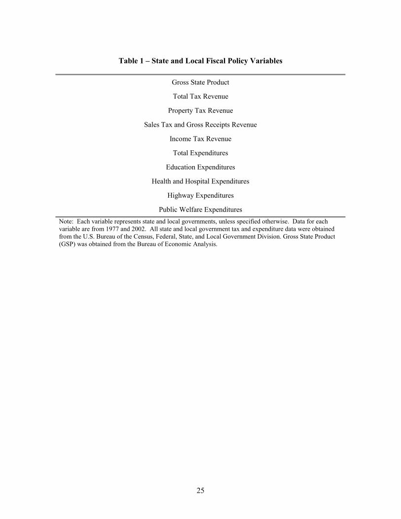
Table 1 – State and Local Fiscal Policy Variables

Gross State Product

Total Tax Revenue

Property Tax Revenue

Sales Tax and Gross Receipts Revenue

Income Tax Revenue

Total Expenditures

Education Expenditures

Health and Hospital Expenditures

Highway Expenditures

Public Welfare Expenditures Note: Each variable represents state and local governments, unless specified otherwise. Data for each variable are from 1977 and 2002. All state and local government tax and expenditure data were obtained from the U.S. Bureau of the Census, Federal, State, and Local Government Division. Gross State Product (GSP) was obtained from the Bureau of Economic Analysis.

26

Table 2: Coefficients of Variation – Fiscal Policies

Variable 1977 2002

Gross State Product 0.19 0.18

Total Tax Revenue 0.22 0.18

Property Tax Revenue 0.44 0.39

Sales Tax and Gross Receipts Revenue 0.28 0.29

Income Tax Revenue 0.57 0.45

Total Expenditures 0.18 0.14

Education Expenditures 0.16 0.12

Health and Hospital Expenditures 0.27 0.41

Highway Expenditures 0.37 0.29

Public Welfare Expenditures 0.43 0.26 Notes: A smaller coefficient of variation in 2002 compared to 1977 suggests convergence, whereas a larger coefficient of variation in 2002 compared to 1977 suggests divergence. See footnote #7 in the text for a description of how the coefficient of variation was calculated. All variables are in real per capita dollars and represent state and local governments, unless specified otherwise. Number of observations for each variable was 48 except for income tax revenue (n=42) and sales tax revenue (n=44).

27

Table 3: Fiscal Policy Convergence - Empirical Results

Dependent Variable: Real Gross State Product average annual growth, 1977-2002 Model β1 λ ρ α No. Obs. Log-likelihood LR stat OLS -0.0121*** 48 188.56 SEM (Wrace) -0.0130*** 0.4860*** 0 48 193.51 9.90*** SAR (Wrace) -0.0115*** 0.3740** 0 48 191.88 6.64*** SEM (Wincome) -0.0130*** 0.4860*** 0 48 193.51 9.90*** SAR (Wincome) -0.0115*** 0.3740** 0 48 191.88 6.64*** SEM (Wage) -0.0130*** 0.486*** 0 48 193.51 9.90*** SAR (Wage) -0.0115*** 0.3740** 0 48 191.88 6.63**

Dependent Variable: Total Tax Revenue average annual growth, 1977-2002 Model β1 λ ρ α No. Obs. Log-likelihood LR stat OLS -0.0127*** 48 199.99 SEM (Wrace) -0.0120*** 0.4460*** 0 48 203.42 6.86*** SAR (Wrace) -0.0098*** 0.3800*** 0 48 202.93 5.88** SEM (Wincome) -0.0120*** 0.4460*** 0 48 203.42 6.86*** SAR (Wincome) -0.0098*** 0.3800*** 0 48 202.93 5.88** SEM (Wage) -0.0120*** 0.4460*** 0 48 203.42 6.84*** SAR (Wage) -0.0098*** 0.3800*** 0 48 202.93 5.86**

Dependent Variable: Property Tax Revenue average annual growth, 1977-2002 Model β1 λ ρ α No. Obs. Log-likelihood LR stat OLS -0.0105*** 48 164.15 SEM (Wrace) -0.0080*** 0.5850*** 0 48 170.09 11.88*** SAR (Wrace) -0.0067*** 0.5630*** 0 48 170.43 12.56*** SEM (Wincome) -0.0080*** 0.5850*** 0 48 170.09 11.88*** SAR (Wincome) -0.0067*** 0.5630*** 0 48 170.43 12.56*** SEM (Wage) -0.0080*** 0.5850*** 0 48 170.09 11.87*** SAR (Wage) -0.0067*** 0.5630*** 0 48 170.43 12.56***

Dependent Variable: Sales Tax and Gross Receipts Revenue average annual growth, 1977-2002 Model β1 λ ρ α No. Obs. Log-likelihood LR stat OLS -0.0043 44 175.97 SEM (Wrace) -0.0041 0.4370*** 0 44 178.58 5.22** SAR (Wrace) -0.0044* 0.4479*** 0 44 179.57 7.20*** SEM (Wincome) -0.0041 0.4370*** 0 44 178.58 5.22** SAR (Wincome) -0.0044* 0.4479*** 0 44 179.57 7.20*** SEM (Wage) -0.0038 0.5490*** 0.25 44 178.69 5.44** SAR (Wage) -0.0043* 0.5589*** 0.25 44 179.76 7.57***

Dependent Variable: Income Tax Revenue average annual growth, 1977-2002 Model β1 λ ρ α No. Obs. Log-likelihood LR stat OLS -0.0135*** 42 128.06 SEM (Wrace) -0.0133*** 0.1020 0 42 128.22 0.32 SAR (Wrace) -0.0129*** 0.1490 0 42 128.41 0.70 SEM (Wincome) -0.0127*** -0.3650 1 42 128.88 1.64 SAR (Wincome) -0.0148*** -0.3960* 1 42 129.34 2.56 SEM (Wage) -0.0133*** -0.8390* 1 42 129.29 2.46 SAR (Wage) -0.0136*** -0.8140* 1 42 129.31 2.49

28

Table 3: Fiscal Policy Convergence - Empirical Results (continued)

Dependent Variable: Total Expenditures average annual growth, 1977-2002 Model β1 λ ρ α No. Obs. Log-likelihood LR stat OLS -0.0155*** 48 207.64 SEM (Wrace) -0.0154*** 0.2210 0.5 48 207.98 0.68 SAR (Wrace) -0.0150*** 0.1630 0.5 48 207.91 0.54 SEM (Wincome) -0.0155*** 0.1780 0.25 48 207.90 0.52 SAR (Wincome) -0.0148*** 0.1030 0 48 207.84 0.40 SEM (Wage) -0.0150*** -0.3760 1 48 207.89 0.49 SAR (Wage) -0.0146*** -0.721 1 48 208.63 1.97

Dependent Variable: Education Expenditures average annual growth, 1977-2002 Model β1 λ ρ α No. Obs. Log-likelihood LR stat OLS -0.0201*** 48 205.77 SEM (Wrace) -0.0187*** 0.2920* 0 48 207.04 2.54 SAR (Wrace) -0.0167*** 0.2600* 0 48 207.34 3.14* SEM (Wincome) -0.0189*** 0.3710* 0.25 48 207.08 2.61 SAR (Wincome) -0.0167*** 0.2600* 0 48 207.34 3.14* SEM (Wage) -0.0187*** 0.2920* 0 48 207.04 2.54 SAR (Wage) -0.0167*** 0.2600* 0 48 207.34 3.15*

Dependent Variable: Health and Hospital Expenditures average annual growth, 1977-2002 Model β1 λ ρ α No. Obs. Log-likelihood LR stat OLS -0.0024 48 137.28 SEM (Wrace) -0.0082 0.3440* 1 48 138.05 1.54 SAR (Wrace) -0.0042 0.2440 1 48 137.77 0.98 SEM (Wincome) -0.0011 -0.0740 0 48 137.35 0.14 SAR (Wincome) -0.0016 -0.0740 0 48 137.36 0.16 SEM (Wage) -0.0013 -0.2090 0.75 48 137.39 0.22 SAR (Wage) -0.0017 -0.2110 0.75 48 137.40 0.25

Dependent Variable: Highway Expenditures average annual growth, 1977-2002 Model β1 λ ρ α No. Obs. Log-likelihood LR stat OLS -0.0174*** 48 170.16 SEM (Wrace) -0.0165*** -0.3200 1 48 170.90 1.48 SAR (Wrace) -0.0184*** -0.3060 1 48 171.51 2.7 SEM (Wincome) -0.0185*** -0.6530*** 1 48 173.21 6.10** SAR (Wincome) -0.0179*** -0.3860* 1 48 171.60 2.88* SEM (Wage) -0.0182*** 0.5900** 1 48 171.52 2.71* SAR (Wage) -0.0178*** 0.3720 1 48 170.59 0.84

Dependent Variable: Public Welfare Expenditures average annual growth, 1977-2002 Model β1 λ ρ α No. Obs. Log-likelihood LR stat OLS -0.0261*** 48 161.73 SEM (Wrace) -0.0256*** -0.7930*** 0.75 48 164.48 5.50** SAR (Wrace) -0.0271*** -0.3840* 0.5 48 163.41 3.36* SEM (Wincome) -0.0257*** -0.2720 0 48 162.44 1.42 SAR (Wincome) -0.0242*** 0.2960* 1 48 163.30 3.14* SEM (Wage) -0.0257*** -0.2720 0 48 162.44 1.41 SAR (Wage) -0.0284*** -0.9940*** 0.75 48 164.89 6.33** Notes: *** denotes significance at 1%, ** at 5%, and * at 10%. All regressions were estimated with a constant term, not reported. SEM is the spatial error model and SAR is the spatial autoregressive model. All variables are in real per capita terms and refer to state and local governments, unless specified otherwise. An � = 0 reveals the contiguity weights matrix is used, an 0�� � �� � ������ � ��� �� �

weights matrix is a linear combination of contiguity and income, race or age, and an � = 1 reveals that only the income, race, or age weights matrix is used. See text for description of weights matrices, Wrace, Wincome, and Wage and of the weighting coefficient α.

29