Solutions to the Exercises Linear Algebra · Solutions to the Exercises* on Linear Algebra Laurenz...

Solutions to the Exercises* on

Linear Algebra

Laurenz WiskottInstitut fur Neuroinformatik

Ruhr-Universitat Bochum, Germany, EU

4 February 2017

Contents

1 Vector spaces 4

1.1 Definition . . . . . . . . . . . . . . . . . . . . . . . . . . . . . . . . . . . . . . . . . . . . . . . 4

1.2 Linear combinations . . . . . . . . . . . . . . . . . . . . . . . . . . . . . . . . . . . . . . . . . 4

1.3 Linear (in)dependence . . . . . . . . . . . . . . . . . . . . . . . . . . . . . . . . . . . . . . . . 4

1.3.1 Exercise: Linear independence . . . . . . . . . . . . . . . . . . . . . . . . . . . . . . . 4







1.3.8 Exercise: Linear independence in C3 . . . . . . . . . . . . . . . . . . . . . . . . . . . . 7

1.4 Basis systems . . . . . . . . . . . . . . . . . . . . . . . . . . . . . . . . . . . . . . . . . . . . . 8

1.4.1 Exercise: Vector space of the functions sin(x+ φ) . . . . . . . . . . . . . . . . . . . . . 8

© 2017 Laurenz Wiskott (homepage https://www.ini.rub.de/PEOPLE/wiskott/). This work (except for all figures fromother sources, if present) is licensed under the Creative Commons Attribution-ShareAlike 4.0 International License. To viewa copy of this license, visit http://creativecommons.org/licenses/by-sa/4.0/. Figures from other sources have their owncopyright, which is generally indicated. Do not distribute parts of these lecture notes showing figures with non-free copyrights(here usually figures I have the rights to publish but you don’t, like my own published figures).

Several of my exercises (not necessarily on this topic) were inspired by papers and textbooks by other authors. Unfortunately,I did not document that well, because initially I did not intend to make the exercises publicly available, and now I cannot traceit back anymore. So I cannot give as much credit as I would like to. The concrete versions of the exercises are certainly myown work, though.

In cases where I reuse an exercise in different variants, references may be wrong for technical reasons.*These exercises complement my corresponding lecture notes available at https://www.ini.rub.de/PEOPLE/wiskott/

Teaching/Material/, where you can also find other teaching material such as programming exercises. The table of contents ofthe lecture notes is reproduced here to give an orientation when the exercises can be reasonably solved. For best learning effectI recommend to first seriously try to solve the exercises yourself before looking into the solutions.

1

https://www.ini.rub.de/PEOPLE/wiskott/

http://creativecommons.org/licenses/by-sa/4.0/

https://www.ini.rub.de/PEOPLE/wiskott/Teaching/Material/

https://www.ini.rub.de/PEOPLE/wiskott/Teaching/Material/

1.4.2 Exercise: Basis systems . . . . . . . . . . . . . . . . . . . . . . . . . . . . . . . . . . . 8

1.4.3 Exercise: Dimension of a vector space . . . . . . . . . . . . . . . . . . . . . . . . . . . 8

1.4.4 Exercise: Dimension of a vector space . . . . . . . . . . . . . . . . . . . . . . . . . . . 9

1.5 Representation wrt a basis . . . . . . . . . . . . . . . . . . . . . . . . . . . . . . . . . . . . . . 9

1.5.1 Exercise: Representation of vectors w.r.t. a basis . . . . . . . . . . . . . . . . . . . . . 9

1.5.2 Exercise: Representation of vectors w.r.t. a basis . . . . . . . . . . . . . . . . . . . . . 10

2 Euclidean vector spaces 11

2.1 Inner product . . . . . . . . . . . . . . . . . . . . . . . . . . . . . . . . . . . . . . . . . . . . . 11

2.1.1 Exercise: Inner product for functions . . . . . . . . . . . . . . . . . . . . . . . . . . . . 11

2.1.2 Exercise: Representation of an inner product . . . . . . . . . . . . . . . . . . . . . . . 13

2.2 Norm . . . . . . . . . . . . . . . . . . . . . . . . . . . . . . . . . . . . . . . . . . . . . . . . . 14

2.2.1 Exercise: City-block metric . . . . . . . . . . . . . . . . . . . . . . . . . . . . . . . . . 14

2.2.2 Exercise: Ellipse w.r.t. the city-block metric . . . . . . . . . . . . . . . . . . . . . . . . 14

2.2.3 Exercise: From norm to inner product . . . . . . . . . . . . . . . . . . . . . . . . . . . 15

2.2.4 Exercise: From norm to inner product (concrete) . . . . . . . . . . . . . . . . . . . . . 16

2.3 Angle . . . . . . . . . . . . . . . . . . . . . . . . . . . . . . . . . . . . . . . . . . . . . . . . . 16

2.3.1 Exercise: Angle with respect to an inner product . . . . . . . . . . . . . . . . . . . . . 16



3 Orthonormal basis systems 17

3.1 Definition . . . . . . . . . . . . . . . . . . . . . . . . . . . . . . . . . . . . . . . . . . . . . . . 17

3.1.1 Exercise: Pythagoras’ theorem . . . . . . . . . . . . . . . . . . . . . . . . . . . . . . . 17

3.1.2 Exercise: Linear independence of orthogonal vectors . . . . . . . . . . . . . . . . . . . 18

3.1.3 Exercise: Product of matrices of basis vectors . . . . . . . . . . . . . . . . . . . . . . . 19

3.2 Representation wrt an orthonormal basis . . . . . . . . . . . . . . . . . . . . . . . . . . . . . . 20

3.2.1 Exercise: Writing vectors in terms of an orthonormal basis . . . . . . . . . . . . . . . 20

3.3 Inner product . . . . . . . . . . . . . . . . . . . . . . . . . . . . . . . . . . . . . . . . . . . . . 21

3.3.1 Exercise: Norm of a vector . . . . . . . . . . . . . . . . . . . . . . . . . . . . . . . . . 21

3.3.2 Exercise: Writing polynomials in terms of an orthonormal basis and simplified innerproduct . . . . . . . . . . . . . . . . . . . . . . . . . . . . . . . . . . . . . . . . . . . . 21

3.4 Projection . . . . . . . . . . . . . . . . . . . . . . . . . . . . . . . . . . . . . . . . . . . . . . . 23

3.4.1 Exercise: Projection . . . . . . . . . . . . . . . . . . . . . . . . . . . . . . . . . . . . . 23

3.4.2 Exercise: Is P a projection matrix . . . . . . . . . . . . . . . . . . . . . . . . . . . . . 24

2

3.4.3 Exercise: Symmetry of a projection matrix . . . . . . . . . . . . . . . . . . . . . . . . 25

3.5 Change of basis . . . . . . . . . . . . . . . . . . . . . . . . . . . . . . . . . . . . . . . . . . . . 25

3.5.1 Exercise: Change of basis . . . . . . . . . . . . . . . . . . . . . . . . . . . . . . . . . . 25



3.6 Schmidt orthogonalization process . . . . . . . . . . . . . . . . . . . . . . . . . . . . . . . . . 27

3.6.1 Exercise: Gram-Schmidt orthonormalization . . . . . . . . . . . . . . . . . . . . . . . . 27

3.6.2 Exercise: Gram-Schmidt orthonormalization . . . . . . . . . . . . . . . . . . . . . . . . 28

3.6.3 Exercise: Gram-Schmidt orthonormalization of polynomials . . . . . . . . . . . . . . . 29

4 Matrices 30

4.0.1 Exercise: Matrix as a sum of a symmetric and an antisymmetric matrix . . . . . . . . 30

4.1 Matrix multiplication . . . . . . . . . . . . . . . . . . . . . . . . . . . . . . . . . . . . . . . . . 31

4.2 Matrices as linear transformations . . . . . . . . . . . . . . . . . . . . . . . . . . . . . . . . . 31

4.2.1 Exercise: Antisymmetric matrices yield orthogonal vectors . . . . . . . . . . . . . . . . 31

4.2.2 Exercise: Matrices that preserve the length of all vectors . . . . . . . . . . . . . . . . . 33

4.2.3 Exercise: Derivative as a matrix operation . . . . . . . . . . . . . . . . . . . . . . . . . 33



4.3 Rank of a matrix . . . . . . . . . . . . . . . . . . . . . . . . . . . . . . . . . . . . . . . . . . . 37

4.4 Determinant . . . . . . . . . . . . . . . . . . . . . . . . . . . . . . . . . . . . . . . . . . . . . . 37

4.4.1 Exercise: Determinants . . . . . . . . . . . . . . . . . . . . . . . . . . . . . . . . . . . 37

4.4.2 Exercise: Determinant . . . . . . . . . . . . . . . . . . . . . . . . . . . . . . . . . . . . 38

4.4.3 Exercise: Determinant . . . . . . . . . . . . . . . . . . . . . . . . . . . . . . . . . . . . 39

4.5 Inversion + . . . . . . . . . . . . . . . . . . . . . . . . . . . . . . . . . . . . . . . . . . . . . . 39

4.6 Trace . . . . . . . . . . . . . . . . . . . . . . . . . . . . . . . . . . . . . . . . . . . . . . . . . . 39

4.6.1 Exercise: Trace and determinant of a symmetric matrix . . . . . . . . . . . . . . . . . 39

4.7 Orthogonal matrices . . . . . . . . . . . . . . . . . . . . . . . . . . . . . . . . . . . . . . . . . 40

4.8 Diagonal matrices . . . . . . . . . . . . . . . . . . . . . . . . . . . . . . . . . . . . . . . . . . 40

4.8.1 Exercise: Matrices as transformations . . . . . . . . . . . . . . . . . . . . . . . . . . . 40

4.8.2 Exercise: Matrices as transformations . . . . . . . . . . . . . . . . . . . . . . . . . . . 41

4.8.3 Exercise: Matrices with certain properties . . . . . . . . . . . . . . . . . . . . . . . . . 41

4.9 Eigenvalue equation for symmetric matrices . . . . . . . . . . . . . . . . . . . . . . . . . . . . 42

4.9.1 Exercise: Eigenvectors of a matrix . . . . . . . . . . . . . . . . . . . . . . . . . . . . . 42

3

4.9.2 Exercise: Eigenvalue problem . . . . . . . . . . . . . . . . . . . . . . . . . . . . . . . . 42

4.9.3 Exercise: Eigenvectors of a matrix . . . . . . . . . . . . . . . . . . . . . . . . . . . . . 43

4.9.4 Exercise: Eigenvectors of a matrix of type∑

vivTi . . . . . . . . . . . . . . . . . . . . 44

4.9.5 Exercise: Eigenvectors of a symmetric matrix are orthogonal . . . . . . . . . . . . . . 44

4.10 General eigenvectors . . . . . . . . . . . . . . . . . . . . . . . . . . . . . . . . . . . . . . . . . 45

4.10.1 Exercise: Matrices with given eigenvectors and -values . . . . . . . . . . . . . . . . . . 45

4.10.2 Exercise: From eigenvalues to matrices . . . . . . . . . . . . . . . . . . . . . . . . . . . 46

4.10.3 Exercise: Generalized eigenvalue problem . . . . . . . . . . . . . . . . . . . . . . . . . 48

4.11 Complex eigenvalues . . . . . . . . . . . . . . . . . . . . . . . . . . . . . . . . . . . . . . . . . 49

4.11.1 Exercise: Complex eigenvalues . . . . . . . . . . . . . . . . . . . . . . . . . . . . . . . 49

4.12 Nonquadratic matrices + . . . . . . . . . . . . . . . . . . . . . . . . . . . . . . . . . . . . . . 50

4.13 Quadratic forms + . . . . . . . . . . . . . . . . . . . . . . . . . . . . . . . . . . . . . . . . . . 50

1 Vector spaces

1.1 Definition

1.2 Linear combinations

1.3 Linear (in)dependence

1.3.1 Exercise: Linear independence

Are the following vectors linearly independent? Do they form a basis of the given vector space V ?

(a) v1 =

130

, v2 =

8−20

, V = R3.

(b) f1(x) = x2 + 3x+ 1, f2(x) = 3x2 + 6x, f3(x) = x+ 1, vector space of polynomials of degree 2.



(a) v1 =

(02

), v2 =

(−34

), V = R2.

(b) f1(x) = 2x, f2(x) = −3 + 4x, V = vector space of polynomials of degree 2.



4

(a) v1 =

(02

), v2 =

(31

), V = R2.

Solution: v1 and v2 are obviously linearly independent and then they are also a basis of V = R2 fordimensionality reasons.

(b) f1(x) = x2− 2x− 3, f2(x) = 2x2 + 3x− 5, f3(x) = x− 1, V = vector space of polynomials of degree 2.

Solution: Linear independence of the three vectors can be shown by the proof that no linear com-bination of the three vectors (besides the trivial solution: all coefficients equal 0) results in the zerovector.

0 = a(x2 − 2x− 3) + b(2x2 + 3x− 5) + c(x− 1) (1)

= (a+ 2b)x2 + (−2a+ 3b+ c)x+ (−3a− 5b− c) (2)

⇐⇒ 0 = a+ 2b (3)

∧ 0 = −2a+ 3b+ c (4)

∧ 0 = −3a− 5b− c (5)

⇐⇒ 0 = a+ 2b (6)

∧ 0 = −4a (equations (3) + (4) + (5)) (7)

∧ 0 = −3a− 5b− c (8)

⇐⇒ a = 0 (9)

∧ b = 0 (since a = 0) (10)

∧ c = 0 (since a = 0 and b = 0) . (11)

There is no other solution than the trivial one. Thus, f1–f3 are linearly independent and form a basisof the vector space of polynomials of degree 2 for dimensionality reasons.



(a) v1 =

024

, v2 =

321

, V = R3.

Solution: v1 and v2 are obviously linearly independent, but they are not a basis for dimensionalityreasons. One vector is missing to span the three dimensional space V = R3.

(b) f1(x) = 3x2 − 1, f2(x) = x, f3(x) = 1, V = vector space of polynomials of degree 2.

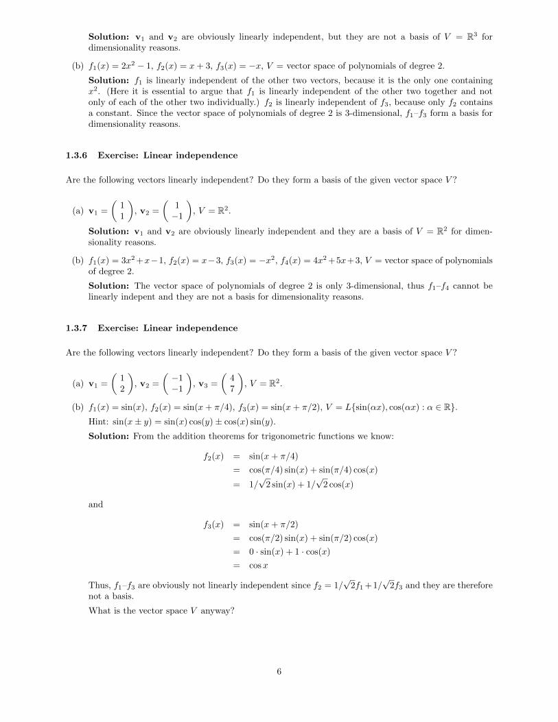
Solution: f1 is linearly independent of the other two vectors, because it is the only one containing x2.(Here it is essential to argue that f1 is linearly independent of the other two together and not only ofeach of the other two individually.) We thus can discard the first vector and only consider the othertwo vectors for linear dependence. But it is quite obvious that f2 and f3 are not linearly dependent.Thus all three vectors are linearly independent. Since the vector space of polynomials of degree 2 is3-dimensional, f1–f3 form a basis for dimensionality reasons.



(a) v1 =

310

, v1 =

1−20

, V = R3.

5

Solution: v1 and v2 are obviously linearly independent, but they are not a basis of V = R3 fordimensionality reasons.

(b) f1(x) = 2x2 − 1, f2(x) = x+ 3, f3(x) = −x, V = vector space of polynomials of degree 2.

Solution: f1 is linearly independent of the other two vectors, because it is the only one containingx2. (Here it is essential to argue that f1 is linearly independent of the other two together and notonly of each of the other two individually.) f2 is linearly independent of f3, because only f2 containsa constant. Since the vector space of polynomials of degree 2 is 3-dimensional, f1–f3 form a basis fordimensionality reasons.



(a) v1 =

(11

), v2 =

(1−1

), V = R2.

Solution: v1 and v2 are obviously linearly independent and they are a basis of V = R2 for dimen-sionality reasons.

(b) f1(x) = 3x2 +x−1, f2(x) = x−3, f3(x) = −x2, f4(x) = 4x2 +5x+3, V = vector space of polynomialsof degree 2.

Solution: The vector space of polynomials of degree 2 is only 3-dimensional, thus f1–f4 cannot belinearly indepent and they are not a basis for dimensionality reasons.



(a) v1 =

(12

), v2 =

(−1−1

), v3 =

(47

), V = R2.

(b) f1(x) = sin(x), f2(x) = sin(x+ π/4), f3(x) = sin(x+ π/2), V = L{sin(αx), cos(αx) : α ∈ R}.Hint: sin(x± y) = sin(x) cos(y)± cos(x) sin(y).

Solution: From the addition theorems for trigonometric functions we know:

f2(x) = sin(x+ π/4)

= cos(π/4) sin(x) + sin(π/4) cos(x)

= 1/√

2 sin(x) + 1/√

2 cos(x)

and

f3(x) = sin(x+ π/2)

= cos(π/2) sin(x) + sin(π/2) cos(x)

= 0 · sin(x) + 1 · cos(x)

= cosx

Thus, f1–f3 are obviously not linearly independent since f2 = 1/√

2f1 +1/√

2f3 and they are thereforenot a basis.

What is the vector space V anyway?

6

1.3.8 Exercise: Linear independence in C3

Are the following vectors in C3 over the field C linearly independent? Do they form a basis?

r1 =

111

, r2 =

1+i+i

, r3 =

1−i−i

. (1)

Solution: The question is, whether there exist three constants a, b, and c in C, which are not all zero, butfor which ar1 + br2 + cr3 = 0 holds. With b =: br + i bi und c =: cr + i ci we find

0 = ar1 + br2 + cr3 (2)(1)⇐⇒ 0 = a+ b+ c (3)

∧ 0 = a+ i b− i c (4)

⇐⇒ a = −b− c (5)

∧ 0 = −b− c+ i b− i c (6)

= b(−1 + i) + c(−1− i) (7)

= (br + i bi)(−1 + i) + (cr + i ci)(−1− i) (8)

= −br + i br − i bi − bi − cr − i cr − i ci + ci (9)

= (−br − bi − cr + ci) + i (+br − bi − cr − ci) (10)

⇔ 0 = −br − bi − cr + ci (11)

= (−bi − cr) + (−br + ci) (12)

∧ 0 = br − bi − cr − ci (13)

= (−bi − cr)− (−br + ci) (14)

⇔ bi = −cr (15)

∧ br = ci (16)

⇐= a = −1− i (17)

∧ b = 1 (18)

∧ c = i , (19)

and verify

ar1 + br2 + cr3 = (−1− i)

111

+

1+i+i

+ i

1−i−i

(20)

=

−1−1−1

+

−i−i−i

+

1+i+i

+

i11

(21)

=

000

. (22)

This shows that the three vectors in C3 are linearly dependent.

The ⇐= in line (17) is needed here, because we are searching for a solution of Equation (2), but we cannotderive a unique solution, i.e. if we set a = −1− i, b = 1, c = i then (2) is true, but from (2) does not followa = −1− i, b = 1, c = i.

One could have suspected that right from the start, because the second and third component are copies ofeach other in all three vectors. This means that the three vectors can only be linearly independent if thevectors shortened by the last component are linearly independent. But since there are no three linearlyindependent vectors in C2 over the field C2, like in R2, the three vectors r1 to r3 must be linearly dependent.

Extra question: What is the dimensionality and a basis of

7

(a) C3 over the field C ?

(b) C3 over the field R ?

1.4 Basis systems

1.4.1 Exercise: Vector space of the functions sin(x+ φ)

Show that the set of functions V = {f(x) = A sin(x + φ)|A ∈ R, φ ∈ [0, 2π]} generates a vector space overthe field of real numbers. Find a basis for V and determine its dimension.

Hint: The addition theorems for trigonometric functions are helpful for the solution, in particular sin(x+y) =sin(x) cos(y) + sin(y) cos(x).

Solution: From the addition theorems for trigonometric functions follows:

f(x) = A sin(x+ φ) = A sin(x) cos(φ) +A sin(φ) cos(x) . (1)

Since A, sin(φ), and cos(φ) are simply real numbers, every f(x) can be written as a linear combination ofsin(x) and cos(x).

On the other hand, every linear combination of sin(x) und cos(x) can be written as A sin(x + φ) and istherefore an element of V , since A(cos(φ), sin(φ))T can realize any pair of two real numbers.

Since the latter also holds for the pairs (1, 0)T and (0, 1)T , the two functions sin(x) and cos(x) are elementsof V .

These three properties make sin(x) and cos(x) a basis of V , which implies that V is a two-dimensional vectorspace.

Extra question: What is the dimensionality and a basis of V = {f(x) = A sin(kx)|A, k ∈ R} over R ?

Extra question: What is is the dimensionality and a basis of V = {f(x) = A exp(iα + x)|A,α ∈ R} overC ?

1.4.2 Exercise: Basis systems

1. Find two different basis systems for the vector space of the polynomials of degree 3.

Solution: The most obvious basis is 1, x, x2, x3. A different basis can be derived from this by simplyadding some of the previous ones, e.g. 1, x+ 1, x2 + 1, x3 + 1.

2. Find a basis for the vector space of symmetric 3×3 matrices.

Solution: For symmetric matrices the diagonal elements can be chosen independently, but opposingoff-diagonal elements are coupled together. Thus, a basis for symmetric 3× 3-matrices, for instance, is 1 0 0

0 0 00 0 0

,

0 1 01 0 00 0 0

,

0 0 10 0 01 0 0

, (1)

0 0 00 1 00 0 0

,

0 0 00 0 10 1 0

,

0 0 00 0 00 0 1

. (2)

1.4.3 Exercise: Dimension of a vector space

Determine the dimension of the following vector spaces.

8

(a) Vector space of real symmetric n× n matrices (for a given n).

Solution: A symmetric n× n matrix has n2 coefficients. However, only the coefficients in the upperright triangle (including the diagonal) can be choosen freely, those in the lower left triangle (withoutthe diagonal) follow from the symmetry condition. Thus, there are n(n + 1)/2 free parameters andthat is the dimension of the vector space of symmetric n× n matrices.

Extra question: What is the dimensionality of real anti-symmetric n× n matrices (for a given n)?

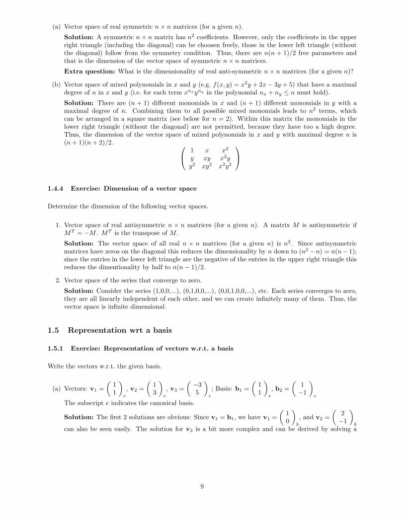
(b) Vector space of mixed polynomials in x and y (e.g. f(x, y) = x2y + 2x− 3y + 5) that have a maximaldegree of n in x and y (i.e. for each term xnxyny in the polynomial nx + ny ≤ n must hold).

Solution: There are (n + 1) different monomials in x and (n + 1) different monomials in y with amaximal degree of n. Combining them to all possible mixed monomials leads to n2 terms, whichcan be arranged in a square matrix (see below for n = 2). Within this matrix the monomials in thelower right triangle (without the diagonal) are not permitted, because they have too a high degree.Thus, the dimension of the vector space of mixed polynomials in x and y with maximal degree n is(n+ 1)(n+ 2)/2. 1 x x2

y xy x2yy2 xy2 x2y2

1.4.4 Exercise: Dimension of a vector space

Determine the dimension of the following vector spaces.

1. Vector space of real antisymmetric n × n matrices (for a given n). A matrix M is antisymmetric ifMT = −M . MT is the transpose of M .

Solution: The vector space of all real n × n matrices (for a given n) is n2. Since antisymmetricmatrices have zeros on the diagonal this reduces the dimensionality by n down to (n2−n) = n(n− 1);since the entries in the lower left triangle are the negative of the entries in the upper right triangle thisreduces the dimentionality by half to n(n− 1)/2.

2. Vector space of the series that converge to zero.

Solution: Consider the series (1,0,0,...), (0,1,0,0,...), (0,0,1,0,0,...), etc. Each series converges to zero,they are all linearly independent of each other, and we can create infinitely many of them. Thus, thevector space is infinite dimensional.

1.5 Representation wrt a basis

1.5.1 Exercise: Representation of vectors w.r.t. a basis

Write the vectors w.r.t. the given basis.

(a) Vectors: v1 =

(11

)e

, v2 =

(13

)e

, v3 =

(−35

)e

; Basis: b1 =

(11

)e

, b2 =

(1−1

)e

The subscript e indicates the canonical basis.

Solution: The first 2 solutions are obvious: Since v1 = b1, we have v1 =

(10

)b

, and v2 =

(2−1

)b

can also be seen easily. The solution for v3 is a bit more complex and can be derived by solving a

9

linear system of equations. (−35

)e

= a

(11

)e

+ b

(1−1

)e

(1)

⇐⇒ −3 = a+ b (2)

∧ 5 = a− b (3)

⇐⇒ 2 = 2a (1st + 2nd equation) (4)

∧ 5 = a− b (5)

⇐⇒ a = 1 (6)

∧ b = −4 (since a = 1) (7)

⇐⇒ v3 =

(1−4

)b

. (8)

(b) Vector: f(x) = −3x2 + 23x− 1; Basis: x2, x, 1

Solution: This is very easy to solve, since the basis consists of the pure monomials. One simply stacksthe coefficients of the polynomial, which yields

f(x) =

−323−1

. (9)

(c) Vector: g(x) = (x+ 1)(x− 1); Basis: x3, x2 + 1, x, 1.

Solution: This, too, is easy to solve, once the polynomial is multiplied out.

g(x) = (x+ 1)(x− 1) = x2 − 1 =

010−2

. (10)

1.5.2 Exercise: Representation of vectors w.r.t. a basis

Write the vectors w.r.t. the given basis.

(a) Vector: v =

123

e

; Basis: b1 =

1−10

e

, b2 =

10−1

e

, b3 =

001

e

The subscript e indicates the canonical basis.

Solution: This can be easily solved in a cascade. First one determines the contribution of b1 to getthe second component, since b1 is the only basis vector that contributes there. Then one determinesthe contribution of b2 to get the first component, since b3 does not contribute there. Finally onedetermines the contribution of b3 to get the third component. This way one finds

v =

−236

b

.

(b) Vector: h(x) = 3x2 − 2x− 3; Basis: x2 − x+ 1, x+ 2, x2 − 1

Solution: This example is difficult to solve directly. Thus, one has to solve a system of linear

10

differential equations.

3x2 − 2x− 3 = a(x2 − x+ 1) + b(x+ 2) + c(x2 − 1) (1)

= (a+ c)x2 + (−a+ b)x+ (a+ 2b− c) (2)

⇐⇒ 3 = a+ c (3)

∧ −2 = −a+ b (4)

∧ −3 = a+ 2b− c (5)

⇐⇒ 3 = a+ c (6)

∧ 1 = b+ c (1st + 2nd equation) (7)

∧ −6 = 2b− 2c (3rd − 1st equation) (8)

⇐⇒ 3 = a+ c (9)

∧ 1 = b+ c (10)

∧ −8 = −4c (3rd − 2×2nd equation) (11)

⇐⇒ a = 1 (since c = 2) (12)

∧ b = −1 (since c = 2) (13)

∧ c = 2 (14)

⇐⇒ h =

1−12

. (15)

2 Euclidean vector spaces

2.1 Inner product

2.1.1 Exercise: Inner product for functions

Consider the space of real continuous functions defined on [−1, 1] for which∫ 1

−1[f(x)]2 dx exists. Let theinner product be

(f, g) :=

∫ 1

−1w(x)f(x)g(x) dx , (1)

with an arbitrary positive weighting function

0 < w(x) <∞ . (2)

1. Prove that (1) is indeed an inner product.

11

Solution: We simply have to verify the axioms of the inner product. The first three are trivial.

(λf, g) =

∫ 1

−1w(x)λf(x)g(x) dx (3)

= λ

∫ 1

−1w(x)f(x)g(x) dx (4)

= λ(f, g) . (5)

(f + h, g) =

∫ 1

−1w(x)(f(x) + h(x))g(x) dx (6)

=

∫ 1

−1w(x)f(x)g(x) dx+

∫ 1

−1w(x)h(x)g(x) dx (7)

= (f, g) + (h, g) . (8)

(f, g) =

∫ 1

−1w(x)f(x)g(x) dx (9)

=

∫ 1

−1w(x)g(x)f(x) dx (10)

= (g, f) . (11)

The fourth one is more subtle. We first show (f, f) ≥ 0.

f2(x) ≥ 0 (12)(2)

=⇒ w(x)f2(x) ≥ 0 (13)

=⇒∫ 1

−1w(x)f2(x) dx ≥ 0 (14)

(1)⇐⇒ (f, f) ≥ 0 . (15)

It is also easy to show that (f(x) = 0)⇒ ((f, f) = 0), since

f(x) = 0 (16)

=⇒ w(x)f2(x) = 0 (17)

=⇒∫ 1

−1w(x)f2(x) dx = 0 (18)

(1)⇐⇒ (f, f) = 0 . (19)

Really difficult is the other direction, ((f, f) = 0) ⇒ (f(x) = 0). We can prove that by showing theinverse direction for the negation, i.e. ¬((f, f) = 0)⇐ ¬(f(x) = 0).

¬(f(x) = 0) means that there is an x0 ∈ [−1, 1], for which f(x0) 6= 0. Because of the continuity of fthere is then also a finite δ-neighborhood around x0 for which f(x) 6= 0, and because of w(x) > 0 follows∫ x0+δ

x0−δ w(x)f2(x) dx > 0 (for simplicity I have assumed here that x0 is an inner point, but something

analogous hold for a point at the border). Furthermore, one can easily show that∫ baw(x)f2(x) dx ≥ 0

for arbitrary −1 ≤ a < b ≤ 1, compare proof above for (f, f) ≥ 0. But that means that the positivecontribution of the integral around x0 cannot be compensated for by a negative contribution at another

location. Therefore∫ 1

−1 w(x)f2(x) dx = (f, f) > 0. Thus we have shown that ¬((f, f) = 0) ⇐¬(f(x) = 0), and ((f, f) = 0) ⇒ (f(x) = 0) holds as well. Since we have shown the other directionalready farther above, we have proven

(f, f) = 0 ⇐⇒ f(x) = 0 , (20)

as required. (1) therefore is a scalar product.

2. Show whether (1) is an inner product also for non-continuous functions.

12

Solution: We show that (1) is no inner product by finding a counter example. If, for instance,f(0) = 1 and f(x) = 0 otherwise, then f is obviously not the zero-function, but still the weightedintegral over f(x) vanishes, because f differs from zero only in a single point. Thus, the fourth axiomis violated and we don’t have an inner product anymore.

3. Show whether (1) is an inner product for continuous functions even if the weighting function is positiveonly in the inner of the interval, i.e. if w(x) > 0∀x ∈ (−1, 1) but w(±1) = 0.

Solution: The first properties of the inner product are not critical. Only the fourth one requiresfurther consideration. With the new weighting function, a difference to the inner product above couldonly be at the border. If w(−1) = 0, then f(−1) could be non-zero without contributing to the integral.However, since f has to be continuous, f(x) 6= 0 would then also hold in a small δ-neighborhood, andin this neighborhood w(x) > 0 holds, so that there we would indeed get a positive contribution to theintegral. This means, the fourth axiom is still valid and (1) an inner product.

2.1.2 Exercise: Representation of an inner product

Let V be an N -dimensional vector space over R and let {bi} with i = 1, ..., N be a basis. Let x = (x1, ..., xN )Tband y = (y1, ..., yN )Tb be the representations of two vectors x,y ∈ V with respect to the basis {bi}. Showthat:

(x,y) = xTAy . (1)

where A is an N ×N -matrix.

Solution: Since x and y are representations of x and y with respect to the basis bi, we have x =∑Ni=1 xibi

and y =∑Ni=1 yibi. With this we get

(x,y) =

∑i

xibi,∑j

yjbj

(2)

=∑i,j

xi (bibj)︸︷︷︸Aij

yj (3)

= xTAy . (4)

It is interesting that this holds no matter what the original vector space and inner product are. Thus, theintuition we have developed for the Euclidean space generalized to any other vector space and inner product,if we consider the representations wrt the inner product.

Extra question: Write the following expressions in component notation and determine their data type(scalar, column or row vector, or matrix):

(a) xTy

(b) Ay

(c) AB

(d) ABC

(e) xTABCy

(f) xyT

(g) xy

13

2.2 Norm

2.2.1 Exercise: City-block metric

The norm of the city-block metric is defined as:

‖x‖CB :=∑i

|xi|

Prove that this actually is a norm.

Solution:

Properties 1 and 3 are trivially true. Property 2 holds because

‖x + y‖CB =∑i

|xi + yi| ≤∑i

|xi|+ |yi| =∑i

|xi|+∑j

|yj | = ‖x‖CB + ‖y‖CB . (1)

2.2.2 Exercise: Ellipse w.r.t. the city-block metric

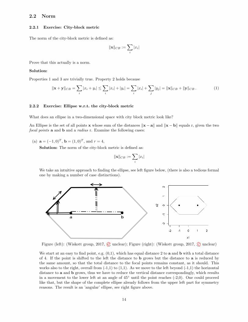
What does an ellipse in a two-dimensional space with city block metric look like?

An Ellipse is the set of all points x whose sum of the distances ‖x− a‖ and ‖x− b‖ equals r, given the twofocal points a and b and a radius r. Examine the following cases:

(a) a = (−1, 0)T , b = (1, 0)T , and r = 4,

Solution: The norm of the city-block metric is defined as:

‖x‖CB :=∑i

|xi|

We take an intuitive approach to finding the ellipse, see left figure below, (there is also a tedious formalone by making a number of case distinctions).

Figure (left): (Wiskott group, 2017, © unclear); Figure (right): (Wiskott group, 2017, © unclear)

We start at an easy to find point, e.g. (0,1), which has equal distance 2 to a and b with a total distanceof 4. If the point is shifted to the left the distance to b grows but the distance to a is reduced bythe same amount, so that the total distance to the focal points remains constant, as it should. Thisworks also to the right, overall from (-1,1) to (1,1). As we move to the left beyond (-1,1) the horizontaldistance to a and b grows, thus we have to reduce the vertical distance correspondingly, which resultsin a movement to the lower left at an angle of 45◦ until the point reaches (-2,0). One could proceedlike that, but the shape of the complete ellipse already follows from the upper left part for symmetryreasons. The result is an ’angular’ ellipse, see right figure above.

14

(b) a = (1, 1)T , b = (2, 2)T , and r = 4.

Solution:

Figure (left): (Wiskott group, 2017, © unclear); Figure (right): (Wiskott group, 2017, © unclear)

One can find the solution in a similar way as described in (a), see left figure above. We start at aneasy to find point, e.g. (1,0). If you move from (1,0) to the right, you see that the distance to a grows,but the distance to b is reduced by the same amount, so that the total distance remains constant, asit should. However, beyond (2,0), the distance to b also grows. Therefore, the point has to be shiftedupwards at the same rate as it move to the right to keep the total distance to the focal points constant.The point thus moves at an angle of 45◦ to the abscissa until it reaches (3,1). One can proceed in thisway, but the complete ellipse already follows from these two parts for symmetry reasons. The result isan octagon, see right figure above.

Extra question: What is the pattern here? How does an ellipse look in general?

Extra question: How does an ellipse with large radius look?

Extra question: How does an ellipse with smallest possible radius look?

Extra question: Does an ellipse uniquely define its focal points?

Extra question: How does a circle look for the maximum norm ‖x‖ := maxi |xi|?

Extra question: How does an ellipse look for the maximum norm ‖x‖ := maxi |xi|?

2.2.3 Exercise: From norm to inner product

Every inner product (·, ·) defines a norm by ‖x‖ =√

(x,x). Show that a norm can also define an inner productover the field R (if it exists, which is the case if the parallelogram law ‖x + y‖2 + ‖x−y‖2 = 2(‖x‖2 + ‖y‖2)holds).

Hint: Make the ansatz (x + y,x + y) = . . . and derive a formula for the inner product given a norm.

15

Solution:

(x + y,x + y) = (x,x + y) + (y,x + y) (1)

= (x,x) + (x,y) + (y,x) + (y,y) (2)

= (x,x) + 2(x,y) + (y,y) (3)

⇐⇒ (x,y) =1

2((x + y,x + y)− (x,x)− (y,y)) (4)

=1

2

(‖x + y‖2 − ‖x‖2 − ‖y‖2

). (5)

Thus, given a norm ‖x‖, a corresponding inner product can be derived with:

(x,y) :=1

2

(‖x + y‖2 − ‖x‖2 − ‖y‖2

). (6)

Alternatively, one can also use

(x,y) :=1

4

(‖x + y‖2 − ‖x− y‖2

), (7)

known as the polarization identity (D: Polarisationsidentitat)

See also http://en.wikipedia.org/wiki/Parallelogram_law.

Extra question: What is the inner product for the city-block metric?

Extra question: Does the parallelogram law hold for the maximum norm ‖x‖∞ := maxi(|xi|)?

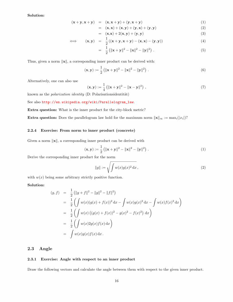
2.2.4 Exercise: From norm to inner product (concrete)

Given a norm ‖x‖, a corresponding inner product can be derived with

(x,y) :=1

2

(‖x + y‖2 − ‖x‖2 − ‖y‖2

). (1)

Derive the corresponding inner product for the norm

‖g‖ :=

√∫w(x)g(x)2 dx , (2)

with w(x) being some arbitrary strictly positive function.

Solution:

(g, f) =1

2

(‖g + f‖2 − ‖g‖2 − ‖f‖2

)=

1

2

(∫w(x)(g(x) + f(x))2 dx−

∫w(x)g(x)2 dx−

∫w(x)f(x)2 dx

)=

1

2

(∫w(x)

((g(x) + f(x))2 − g(x)2 − f(x)2

)dx

)=

1

2

(∫w(x)2g(x)f(x) dx

)=

∫w(x)g(x)f(x) dx .

2.3 Angle

2.3.1 Exercise: Angle with respect to an inner product

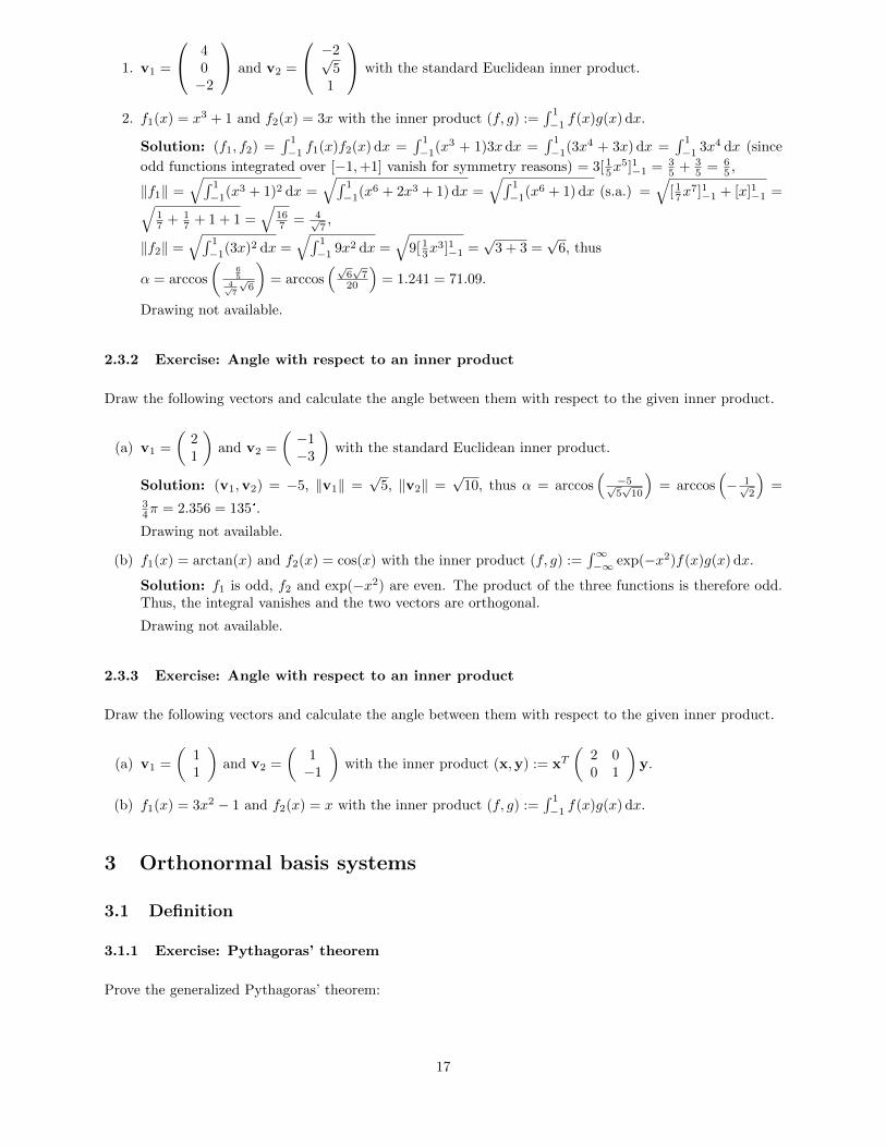
Draw the following vectors and calculate the angle between them with respect to the given inner product.

16

http://en.wikipedia.org/wiki/Parallelogram_law

1. v1 =

40−2

and v2 =

−2√5

1

with the standard Euclidean inner product.

2. f1(x) = x3 + 1 and f2(x) = 3x with the inner product (f, g) :=∫ 1

−1 f(x)g(x) dx.

Solution: (f1, f2) =∫ 1

−1 f1(x)f2(x) dx =∫ 1

−1(x3 + 1)3xdx =∫ 1

−1(3x4 + 3x) dx =∫ 1

−1 3x4 dx (since

odd functions integrated over [−1,+1] vanish for symmetry reasons) = 3[ 15x5]1−1 = 3

5 + 35 = 6

5 ,

‖f1‖ =√∫ 1

−1(x3 + 1)2 dx =√∫ 1

−1(x6 + 2x3 + 1) dx =√∫ 1

−1(x6 + 1) dx (s.a.) =√

[ 17x7]1−1 + [x]1−1 =√

17 + 1

7 + 1 + 1 =√

167 = 4√

7,

‖f2‖ =√∫ 1

−1(3x)2 dx =√∫ 1

−1 9x2 dx =√

9[ 13x3]1−1 =

√3 + 3 =

√6, thus

α = arccos

(65

4√7

√6

)= arccos

(√6√7

20

)= 1.241 = 71.09.

Drawing not available.



(a) v1 =

(21

)and v2 =

(−1−3

)with the standard Euclidean inner product.

Solution: (v1,v2) = −5, ‖v1‖ =√

5, ‖v2‖ =√

10, thus α = arccos(−5√5√10

)= arccos

(− 1√

2

)=

34π = 2.356 = 135°.


(b) f1(x) = arctan(x) and f2(x) = cos(x) with the inner product (f, g) :=∫∞−∞ exp(−x2)f(x)g(x) dx.

Solution: f1 is odd, f2 and exp(−x2) are even. The product of the three functions is therefore odd.Thus, the integral vanishes and the two vectors are orthogonal.




(a) v1 =

(11

)and v2 =

(1−1

)with the inner product (x,y) := xT

(2 00 1

)y.

(b) f1(x) = 3x2 − 1 and f2(x) = x with the inner product (f, g) :=∫ 1

−1 f(x)g(x) dx.

3 Orthonormal basis systems

3.1 Definition

3.1.1 Exercise: Pythagoras’ theorem

Prove the generalized Pythagoras’ theorem:

17

Let vi, i ∈ {1, ..., N} be pairwise orthogonal vectors. Then∥∥∥∥∥N∑i=1

vi

∥∥∥∥∥2

=

N∑i=1

||vi||2.

holds.

Solution: We can show directly∥∥∥∥∥N∑i=1

vi

∥∥∥∥∥2

=

N∑i=1

vi,

N∑j=1

vj

(1)

=

N∑i,j=1

(vi,vj) (2)

=

N∑i=1

(vi,vi) (because (vi,vj) = 0 if i 6= j) (3)

=

N∑i=1

||vi||2 . (4)

Extra question: Does this also hold for the Manhatten/city-block or maximum norm?

3.1.2 Exercise: Linear independence of orthogonal vectors

Show that N pairwise orthogonal vectors (not permitting the zero vector) are always linearly independent.

Solution: Proof by contradiction: We assume the pairwise orthogonal non-zero vectors vi are linearlydependent. Then there exist factors ai, of which at least one is not zero, so that

∑i aivi = 0. From this

follows

0 =∑i

aivi (1)

=⇒ 0 =

(∑i

aivi,vj

)∀j (2)

=∑i

ai(vi,vj) ∀j (3)

= aj(vj ,vj) ∀j (since the vectors are orthogonal) (4)

⇐⇒ 0 = aj ∀j (since the vectors have finite norm) , (5)

which is a contradiction to the assumption. Thus, the assumption is not true and all orthogonal vectors arelinearly independent.

18

Ekaterina Kuzminykh (SS 2017) came up with the following solution.

0 =∑i

aivi (6)

⇐⇒ 0 =

∥∥∥∥∥∑i

aivi

∥∥∥∥∥ (7)

=

∑i

aivi,∑j

ajvj

(8)

=∑ij

aiaj (vi,vj) (9)

=∑i

a2i (vi,vi) (since (vi,vj) = 0 for i 6= j) (10)

⇐⇒ 0 = ai ∀i (since the vectors have finite norm) . (11)

Extra question: Does this also hold for vectors with a pairwise angle of 80° (or 10°)?

Extra question: Does this also hold for vectors with a pairwise angles αij with 80 < αij < 100 (or30 < αij < 150)?

3.1.3 Exercise: Product of matrices of basis vectors

Let {bi}, i = 1, ..., N , be an orthonormal basis and 1N indicate the N -dimensional identity matrix.

1. Show that (b1,b2, ...,bN )T (b1,b2, ...,bN ) = 1N . Does the result also hold if one only takes the firstN − 1 basis vectors? If not, try to interpret the resulting matrix.

Solution:

(b1,b2, ...,bN )T (b1,b2, ...,bN ) =

bT1bT2...

bTN

(b1,b2, ...,bN ) = 1N (1)

follows directly from the fact that bTi bj = δij by definition of an orthonormal basis.

Extra question: What happens if one only takes the first N − 1 vectors?

2. Show that (b1,b2, ...,bN )(b1,b2, ...,bN )T = 1N . Does the result also hold if one only takes the firstN − 1 basis vectors? If not, try to interpret the resulting matrix.

Solution: Writing an arbitrary vector v in terms of the basis bi is done by

vb =

v1bv2b. . .vNb

b

=

bT1 v

bT2 v. . .

bTNv

b

=

bT1bT2...

bTN

v . (2)

Writing the vector vb, which is written in terms of the basis bi, in terms of the Euclidean basis againis done by

v =∑i

vibbi = (b1,b2, ...,bN )

v1bv2b. . .vNb

b

= (b1,b2, ...,bN )vb . (3)

19

Combining these two transformations results in

v = (b1,b2, ...,bN )

bT1bT2...

bTN

v . (4)

Since this is true for any vector v, we conclude that

(b1,b2, ...,bN )(b1,b2, ...,bN )T = (b1,b2, ...,bN )

bT1bT2...

bTN

= 1N . (5)

Extra question: What happens if one only takes the first N − 1 vectors?

3.2 Representation wrt an orthonormal basis

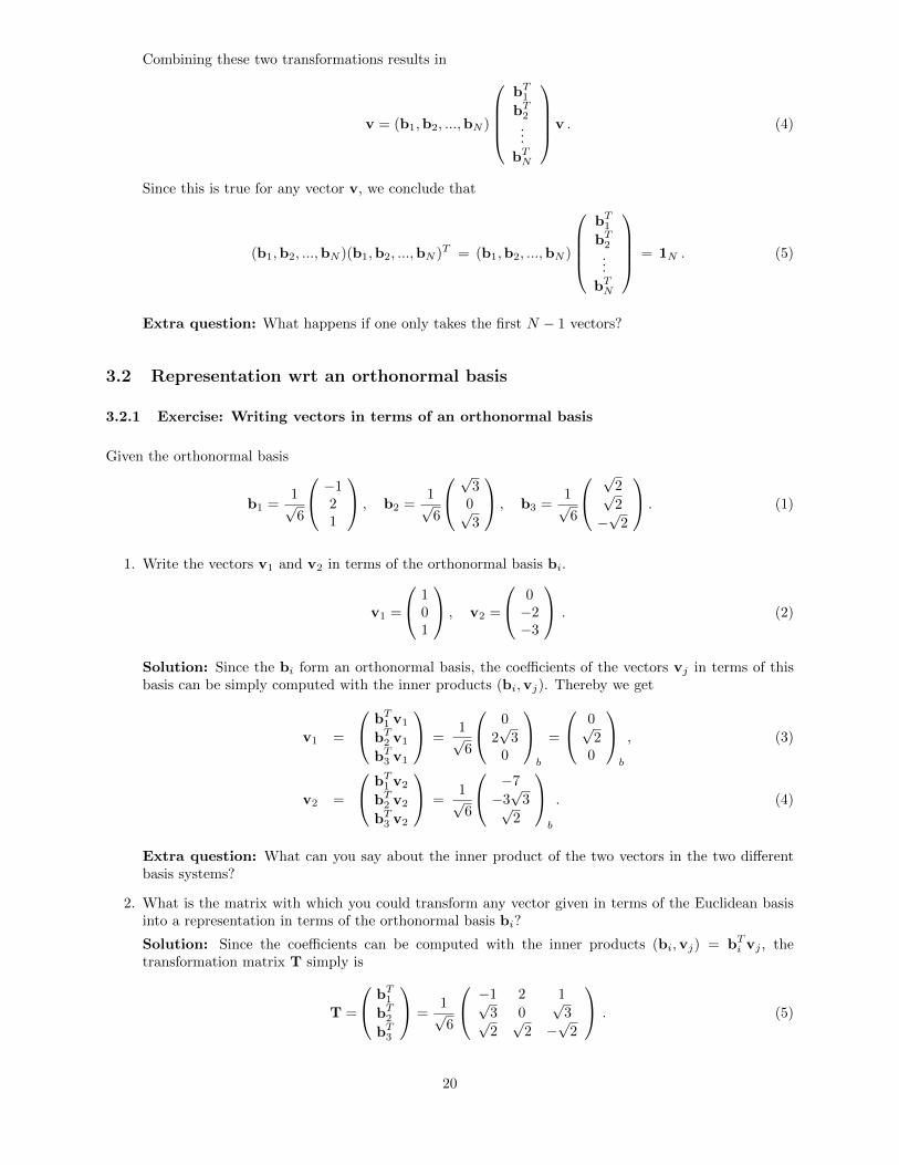
3.2.1 Exercise: Writing vectors in terms of an orthonormal basis

Given the orthonormal basis

b1 =1√6

−121

, b2 =1√6

√30√3

, b3 =1√6

√2√2

−√

2

. (1)

1. Write the vectors v1 and v2 in terms of the orthonormal basis bi.

v1 =

101

, v2 =

0−2−3

. (2)

Solution: Since the bi form an orthonormal basis, the coefficients of the vectors vj in terms of thisbasis can be simply computed with the inner products (bi,vj). Thereby we get

v1 =

bT1 v1

bT2 v1

bT3 v1

=1√6

0

2√

30

b

=

0√2

0

b

, (3)

v2 =

bT1 v2

bT2 v2

bT3 v2

=1√6

−7

−3√

3√2

b

. (4)

Extra question: What can you say about the inner product of the two vectors in the two differentbasis systems?

2. What is the matrix with which you could transform any vector given in terms of the Euclidean basisinto a representation in terms of the orthonormal basis bi?

Solution: Since the coefficients can be computed with the inner products (bi,vj) = bTi vj , thetransformation matrix T simply is

T =

bT1bT2bT3

=1√6

−1 2 1√3 0

√3√

2√

2 −√

2

. (5)

20

3.3 Inner product

3.3.1 Exercise: Norm of a vector

Let bi, i = 1, ..., N , be an orthonormal basis. Then we have (bi,bj) = δij and

v =

N∑i=1

vibi with vi := (v,bi) ∀v . (1)

Show that

‖v‖2 =

N∑i=1

v2i . (2)

Solution: We can show directly that

‖v‖2 = (v,v) (3)

=

N∑i=1

vibi,

N∑j=1

vjbj

(4)

=

N∑i,j=1

vivj (bi,bj)︸︷︷︸δij

(5)

=

N∑i=1

v2i (bi,bi) (since (bi,bj) = 0 for i 6= j) (6)

=

N∑i=1

v2i (since the basis vectors are normalized to 1) . (7)

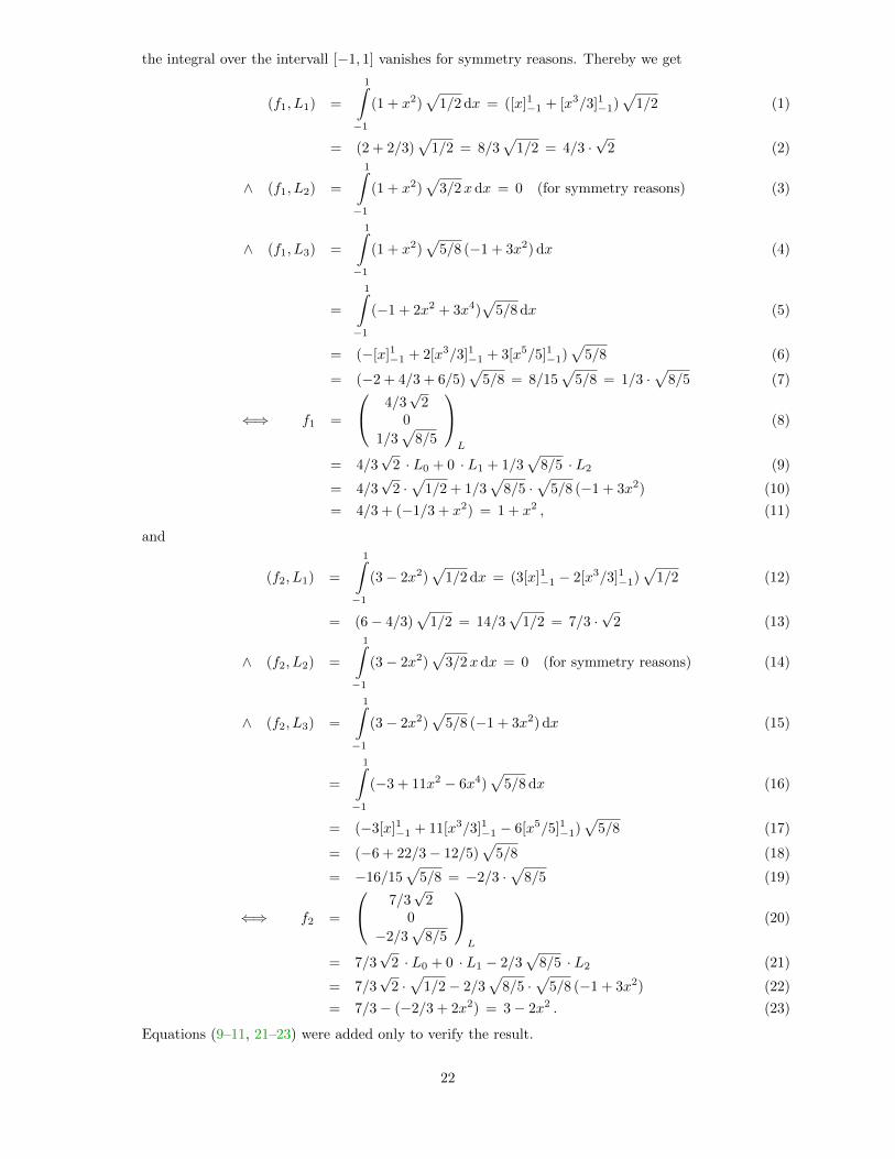
3.3.2 Exercise: Writing polynomials in terms of an orthonormal basis and simplified innerproduct

The normalized Legendre polynomials

L0 =√

1/2 , L1 =√

3/2x , L2 =√

5/8 (−1 + 3x2)

form an orthonormal basis of the vector space of polynomials of degree 2 with respect to the inner product

(f, g) =

1∫−1

f(x)g(x) dx .

1. Write the following polynomials in terms of the basis L0, L1, L2:

f1(x) = 1 + x2 , f2(x) = 3− 2x2 .

Verify the result.

Solution: Since the Li form an orthonormal basis, the coefficients of the vectors fj in terms of thisbasis can be simply computed with the inner products (fi, Lj). Note that if fi×Lj is an odd function,

21

the integral over the intervall [−1, 1] vanishes for symmetry reasons. Thereby we get

(f1, L1) =

1∫−1

(1 + x2)√

1/2 dx = ([x]1−1 + [x3/3]1−1)√

1/2 (1)

= (2 + 2/3)√

1/2 = 8/3√

1/2 = 4/3 ·√

2 (2)

∧ (f1, L2) =

1∫−1

(1 + x2)√

3/2x dx = 0 (for symmetry reasons) (3)

∧ (f1, L3) =

1∫−1

(1 + x2)√

5/8 (−1 + 3x2) dx (4)

=

1∫−1

(−1 + 2x2 + 3x4)√

5/8 dx (5)

= (−[x]1−1 + 2[x3/3]1−1 + 3[x5/5]1−1)√

5/8 (6)

= (−2 + 4/3 + 6/5)√

5/8 = 8/15√

5/8 = 1/3 ·√

8/5 (7)

⇐⇒ f1 =

4/3√

20

1/3√

8/5

L

(8)

= 4/3√

2 · L0 + 0 · L1 + 1/3√

8/5 · L2 (9)

= 4/3√

2 ·√

1/2 + 1/3√

8/5 ·√

5/8 (−1 + 3x2) (10)

= 4/3 + (−1/3 + x2) = 1 + x2 , (11)

and

(f2, L1) =

1∫−1

(3− 2x2)√

1/2 dx = (3[x]1−1 − 2[x3/3]1−1)√

1/2 (12)

= (6− 4/3)√

1/2 = 14/3√

1/2 = 7/3 ·√

2 (13)

∧ (f2, L2) =

1∫−1

(3− 2x2)√

3/2xdx = 0 (for symmetry reasons) (14)

∧ (f2, L3) =

1∫−1

(3− 2x2)√

5/8 (−1 + 3x2) dx (15)

=

1∫−1

(−3 + 11x2 − 6x4)√

5/8 dx (16)

= (−3[x]1−1 + 11[x3/3]1−1 − 6[x5/5]1−1)√

5/8 (17)

= (−6 + 22/3− 12/5)√

5/8 (18)

= −16/15√

5/8 = −2/3 ·√

8/5 (19)

⇐⇒ f2 =

7/3√

20

−2/3√

8/5

L

(20)

= 7/3√

2 · L0 + 0 · L1 − 2/3√

8/5 · L2 (21)

= 7/3√

2 ·√

1/2− 2/3√

8/5 ·√

5/8 (−1 + 3x2) (22)

= 7/3− (−2/3 + 2x2) = 3− 2x2 . (23)

Equations (9–11, 21–23) were added only to verify the result.

22

2. Calculate the inner product (f1, f2) first directly with the integral and then based on the coefficientsof the vectors written in terms of the basis L0, L1, L2.

Solution: We calculate directly

(f1, f2) =

1∫−1

(1 + x2)(3− 2x2)dx =

1∫−1

(3 + x2 − 2x4)dx (24)

= 3[x]1−1 + [x3/3]1−1 − 2[x5/5]1−1 (25)

= 6 + 2/3− 4/5 = 6− 2/15 = 88/15 , (26)

(f1, f2) =

4/3√

20

1/3√

8/5

T

L

7/3√

20

−2/3√

8/5

L

(27)

= 4/3√

2 · 7/3√

2− 1/3√

8/5 · 2/3√

8/5 (28)

=4 · 7 · 2

3 · 3− 2 · 8

3 · 3 · 5=

4 · 7 · 10

3 · 3 · 5− 2 · 8

3 · 3 · 5=

264

45=

88

15. (29)

3.4 Projection

3.4.1 Exercise: Projection

1. Project the vector v = (1, 2,−1)T onto the space orthogonal to the vector b1 = (2, 1,−2)T .

Solution: The ’standard’ way would be to construct basis vectors b2 and b3 for the space orthogonalto b1 and then project onto these with v‖ =

∑3i=2(v,bi)bi. Simpler, however, is it to subtract the

projection onto the space spanned by b1. For that we first normalize b1 to obtain

b1 :=1

‖b1‖b1 =

1√(4 + 1 + 4)

21−2

=1

3

21−2

. (1)

v‖ can then be calculated as

v‖ = v − v⊥ = v − (v,b1)b1 (2)

=

12−1

− 1

3(2 + 2 + 2)

1

3

21−2

(3)

=

12−1

− 2

3

21−2

=1

3

−141

. (4)

We verify that v‖ is indeed orthogonal to b1 and that it is shorter than v.

(v‖,b1) =1

9(−2 + 4− 2) = 0 , (5)

‖v‖ = (1 + 4 + 1) = 6 , (6)

‖v‖‖ =1

9(1 + 16 + 1) =

18

9= 2 < 6 = ‖v‖ . (7)

2. Construct a 3×3-matrix P that realizes the projection onto the subspace orthogonal to b1, so thatv‖ = Pv for any vector v.

23

Solution: We start from what we have written above to calculate v‖ and rewrite it with a matrix.

v‖ = v − (v,b1)b1 = v − b1(b1,v) = 13v − b1bT1 v =

(13 − b1b

T1

)︸︷︷︸

P

v (8)

=⇒ P = 13 − b1bT1 =

1 0 00 1 00 0 1

− b11b11 b11b12 b11b13

b12b11 b12b12 b12b13b13b11 b13b12 b13b13

(9)

=

1 0 00 1 00 0 1

− 1

9

4 2 −42 1 −2−4 −2 4

=1

9

5 −2 4−2 8 2

4 2 5

. (10)

We verify that we get the same vector v‖ for v = (1, 2,−1)T as above but with matrix P.

v‖ = Pv =1

9

5 −2 4−2 8 2

4 2 5

12−1

(11)

=1

9

5− 4− 4−2 + 16− 2

4 + 4− 5

=1

9

−3123

=1

3

−141

. (12)

Extra question: What do you notice about the projection matrix?

Extra question: Is that a coincidence or expected?

3. Calculate the product of P with itself, i.e. PP.

Solution: There are different ways to solve this problem.

� The intuitive way is to realize that after we have projected a vector onto a subspace, the projectedvector lies within the subspace and thus projecting it a second time does not make any difference.Thus, we expect PP = P.

� If we want to be more formal we can show that

PP =(13 − b1b

T1

)(13 − b1b

T1

)(13)

= 1313 − 13b1bT1 − b1b

T1 13 + b1 bT1 b1︸︷︷︸

=1

bT1 (14)

= 13 − b1bT1 − b1b

T1 + b1b

T1 = 13 − b1b

T1 = P . (15)

� Finally, one can do it the direct (hard) way by simply multiplying the matrices.

PP =1

9

5 −2 4−2 8 2

4 2 5

1

9

5 −2 4−2 8 2

4 2 5

= ... (16)

Extra question: Is the product of two projection matrices P1 and P2 again a projection matrix?

3.4.2 Exercise: Is P a projection matrix

Determine whether matrix

P =1

5

(1 22 4

)(1)

is a projection matrix or not.

Solution: The defining property of a projection matrix is that you get the same result if you apply it twice,i.e. PP = P. We verify that

PP =1

5 · 5

(1 22 4

)(1 22 4

)=

1

5 · 5

(5 10

10 20

)=

1

5

(1 22 4

)= P . (2)

24

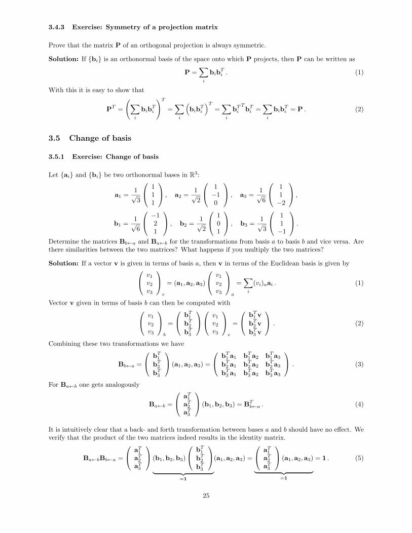
3.4.3 Exercise: Symmetry of a projection matrix

Prove that the matrix P of an orthogonal projection is always symmetric.

Solution: If {bi} is an orthonormal basis of the space onto which P projects, then P can be written as

P =∑i

bibTi . (1)

With this it is easy to show that

PT =

(∑i

bibTi

)T=∑i

(bib

Ti

)T=∑i

bTiTbTi =

∑i

bibTi = P . (2)

3.5 Change of basis

3.5.1 Exercise: Change of basis

Let {ai} and {bi} be two orthonormal bases in R3:

a1 =1√3

111

, a2 =1√2

1−10

, a3 =1√6

11−2

,

b1 =1√6

−121

, b2 =1√2

101

, b3 =1√3

11−1

.

Determine the matrices Bb←a and Ba←b for the transformations from basis a to basis b and vice versa. Arethere similarities between the two matrices? What happens if you multiply the two matrices?

Solution: If a vector v is given in terms of basis a, then v in terms of the Euclidean basis is given by v1v2v3

e

= (a1,a2,a3)

v1v2v3

a

=∑i

(vi)aai . (1)

Vector v given in terms of basis b can then be computed with v1v2v3

b

=

bT1bT2bT3

v1v2v3

e

=

bT1 v

bT2 v

bT3 v

. (2)

Combining these two transformations we have

Bb←a =

bT1bT2bT3

(a1,a2,a3) =

bT1 a1 bT1 a2 bT1 a3



. (3)

For Ba←b one gets analogously

Ba←b =

aT1aT2aT3

(b1,b2,b3) = BTb←a . (4)

It is intuitively clear that a back- and forth transformation between bases a and b should have no effect. Weverify that the product of the two matrices indeed results in the identity matrix.

Ba←bBb←a =

aT1aT2aT3

(b1,b2,b3)

bT1bT2bT3

︸︷︷︸

=1

(a1,a2,a3) =

aT1aT2aT3

(a1,a2,a3)

︸︷︷︸=1

= 1 . (5)

25

For the concrete bases given above we find with (3)

Bb←a =

√

2/9 −√

3/4 −√

1/36√2/3

√1/4 −

√1/12√

1/9 0√

8/9

= BTa←b (6)

and verify that

Ba←bBb←a =

√

2/9√

2/3√

1/9

−√

3/4√

1/4 0

−√

1/36 −√

1/12√

8/9

√

2/9 −√

3/4 −√

1/36√2/3

√1/4 −

√1/12√

1/9 0√

8/9

= 1 . (7)

Extra question: What would change if the basis would not be orthonormal?

Extra question: How can you generalize this concept of change of basis to vector spaces of polynomials ofdegree 2?


Consider {ai} and {bi}, where

a1 =

111

,a2 =

1−10

,a3 =

11−2

,

b1 =1√6

−121

,b2 =1√2

101

,b3 =1√3

11−1

.

1. Are {ai} and {bi} an orthonormal basis of R3? If not, make them orthonormal.

2. Find the transformation matrix Bb←a.

3. Find the inverse of matrix Bb←a.


Let {ai} and {bi} be two orthonormal bases in R2:

a1 =1√2

(11

), a2 =

1√2

(1−1

), b1 =

1√5

(−1

2

), b2 =

1√5

(21

). (1)

Write the vector

v =

(2−3

)a

, (2)

which is given in terms of the basis a, in terms of basis b.

Solution: First we determine the vector in the Euclidean basis.

v =

(2−3

)a

= 2a1 − 3a2 =1√2

(22

)− 1√

2

(3−3

)=

1√2

(−1

5

). (3)

Then we write this vector wrt basis b.

v =

(v1v2

)b

=

(bT1 v

bT2 v

)b

=1√10

(113

)b

. (4)

26

3.6 Schmidt orthogonalization process

3.6.1 Exercise: Gram-Schmidt orthonormalization

Construct an orthonormal basis for the space spanned by the vectors

v1 =

10−2

, v2 =

210

, v3 =

112

.

Solution: There is something suspicious here. Either the three vectors are linearly independent, then theEuclidean basis (1, 0, 0)T , (0, 1, 0)T , (0, 0, 1)T would do, or they are linearly dependent, then one of the threevectors can be ignored. With some guessing one sees that v3 = v2−v1, so the problem reduces to finding abasis for the first two vectors. We apply the Gram-Schmidt orthonormalization to obtain the basis vectorsb1 and b2.

‖v1‖ =√

1 + 0 + 4 =√

5 , (1)

b1 :=v1

‖v1‖=

1√5

10−2

, (2)

b2 := v2 − (v2,b1)b1 (3)

=

210

− 1√5

(2 + 0 + 0)1√5

10−2

(4)

=

210

− 2

5

10−2

=1

5

854

, (5)

‖b2‖ =√

(64 + 25 + 16)/5 =√

105/5 , (6)

b2 :=b2

‖b2‖=

5√105· 1

5

854

=1√105

854

. (7)

Now, if one has not guessed that v3 can be expressed as a linear combination of the other two vectors butproceeds with the Gram-Schmidt procedure, one gets the following.

b3 = v3 − (v3,b1)b1 − (v3,b2)b2 (8)

=

112

− 1√5

(1 + 0− 4)1√5

10−2

− 1√105

(8 + 5 + 8)1√105

854

(9)

=

112

− −3

5

10−2

− 21

105

854

(10)

=1

5

5510

+1

5

30−6

− 1

5

854

=1

5

000

= 0 . (11)

Thus, it becomes apparent that v3 is linearly dependent on v1 and v2 and is therefore redundant. So weare done and the basis is b1 and b2. It is easy to see that the two vectors are normalized and orthogonal.

27

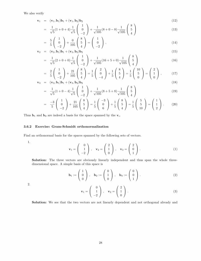
We also verify

v1 = (v1,b1)b1 + (v1,b2)b2 (12)

=1√5

(1 + 0 + 4)1√5

10−2

+1√105

(8 + 0− 8)1√105

854

(13)

=5

5

10−2

+0

105

854

=

10−2

, (14)

v2 = (v2,b1)b1 + (v2,b2)b2 (15)

=1√5

(2 + 0 + 0)1√5

10−2

+1√105

(16 + 5 + 0)1√105

854

(16)

=2

5

10−2

+21

105

854

=1

5

20−4

+1

5

854

=1

5

1050

=

210

, (17)

v3 = (v3,b1)b1 + (v3,b2)b2 (18)

=1√5

(1 + 0− 4)1√5

10−2

+1√105

(8 + 5 + 8)1√105

854

(19)

=−3

5

10−2

+21

105

854

=1

5

−306

+1

5

854

=1

5

5510

=

112

. (20)

Thus b1 and b2 are indeed a basis for the space spanned by the vi.

3.6.2 Exercise: Gram-Schmidt orthonormalization

Find an orthonormal basis for the spaces spanned by the following sets of vectors.

1.

v1 =

01−2

, v2 =

210

, v3 =

201

. (1)

Solution: The three vectors are obviously linearly independent and thus span the whole three-dimensional space. A simple basis of this space is

b1 :=

100

, b2 :=

010

, b3 :=

001

. (2)

2.

v1 =

01−2

, v2 =

210

. (3)

Solution: We see that the two vectors are not linearly dependent and not orthogonal already and

28

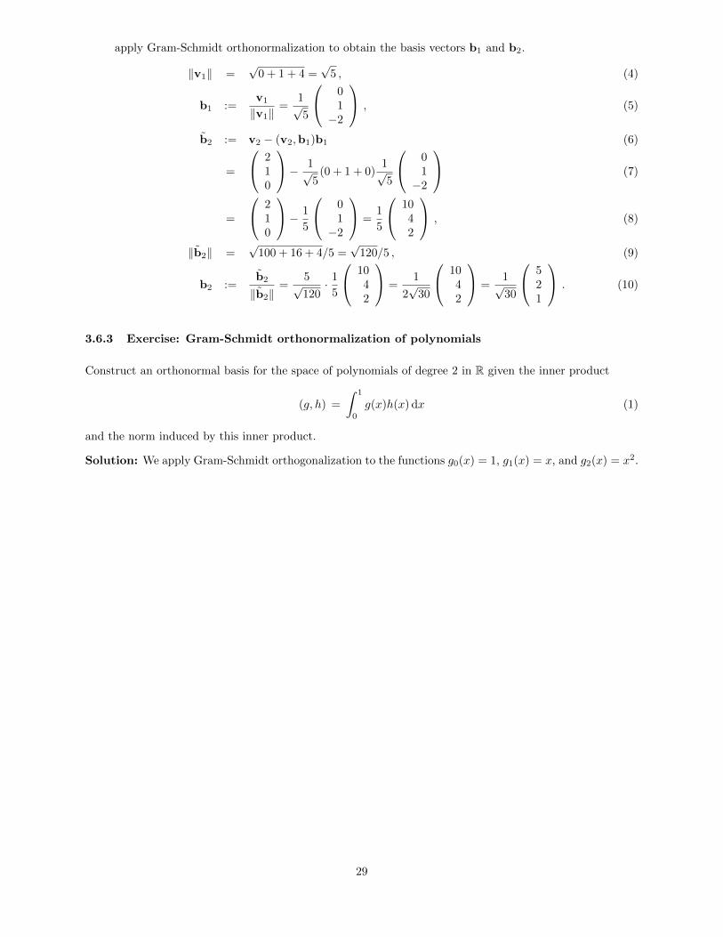
apply Gram-Schmidt orthonormalization to obtain the basis vectors b1 and b2.

‖v1‖ =√

0 + 1 + 4 =√

5 , (4)

b1 :=v1

‖v1‖=

1√5

01−2

, (5)

b2 := v2 − (v2,b1)b1 (6)

=

210

− 1√5

(0 + 1 + 0)1√5

01−2

(7)

=

210

− 1

5

01−2

=1

5

1042

, (8)

‖b2‖ =√

100 + 16 + 4/5 =√

120/5 , (9)

b2 :=b2

‖b2‖=

5√120· 1

5

1042

=1

2√

30

1042

=1√30

521

. (10)

3.6.3 Exercise: Gram-Schmidt orthonormalization of polynomials

Construct an orthonormal basis for the space of polynomials of degree 2 in R given the inner product

(g, h) =

∫ 1

0

g(x)h(x) dx (1)

and the norm induced by this inner product.

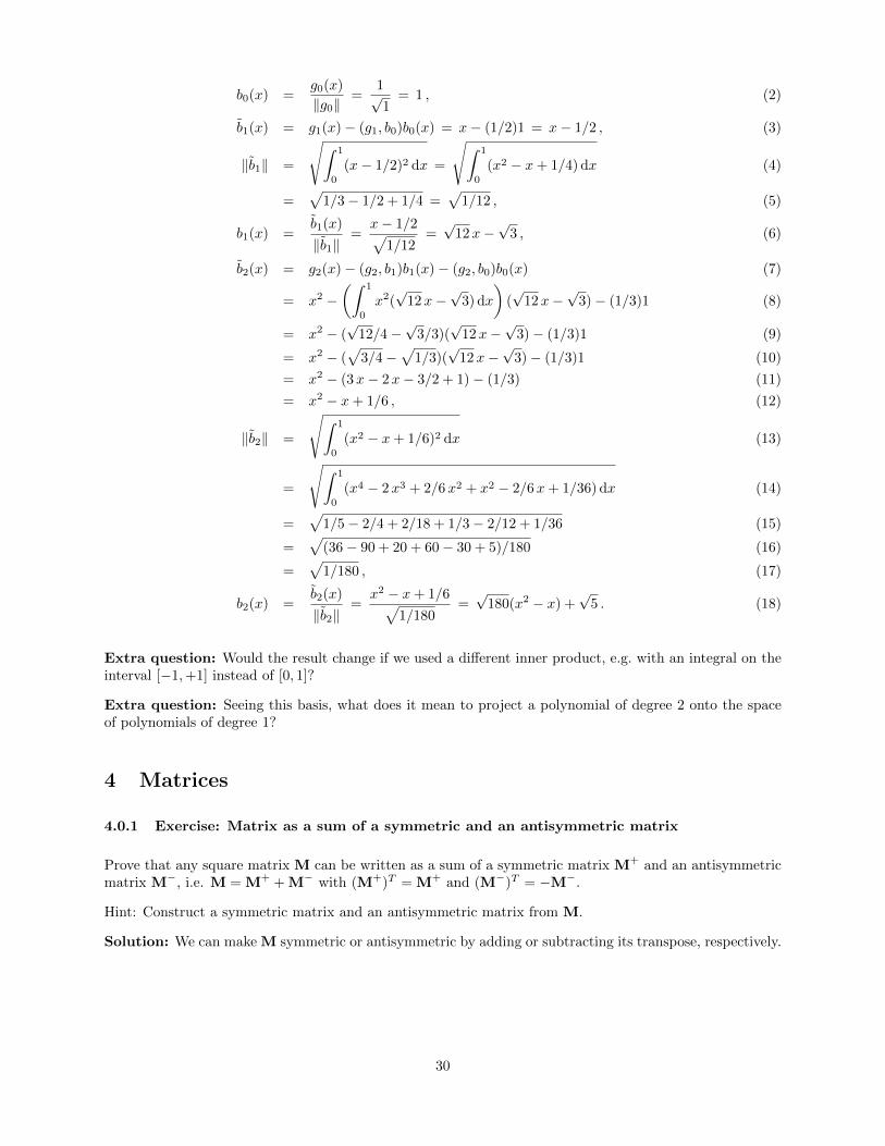
Solution: We apply Gram-Schmidt orthogonalization to the functions g0(x) = 1, g1(x) = x, and g2(x) = x2.

29

b0(x) =g0(x)

‖g0‖=

1√1

= 1 , (2)

b1(x) = g1(x)− (g1, b0)b0(x) = x− (1/2)1 = x− 1/2 , (3)

‖b1‖ =

√∫ 1

0

(x− 1/2)2 dx =

√∫ 1

0

(x2 − x+ 1/4) dx (4)

=√

1/3− 1/2 + 1/4 =√

1/12 , (5)

b1(x) =b1(x)

‖b1‖=

x− 1/2√1/12

=√

12x−√

3 , (6)

b2(x) = g2(x)− (g2, b1)b1(x)− (g2, b0)b0(x) (7)

= x2 −(∫ 1

0

x2(√

12x−√

3) dx

)(√

12x−√

3)− (1/3)1 (8)

= x2 − (√

12/4−√

3/3)(√

12x−√

3)− (1/3)1 (9)

= x2 − (√

3/4−√

1/3)(√

12x−√

3)− (1/3)1 (10)

= x2 − (3x− 2x− 3/2 + 1)− (1/3) (11)

= x2 − x+ 1/6 , (12)

‖b2‖ =

√∫ 1

0

(x2 − x+ 1/6)2 dx (13)

=

√∫ 1

0

(x4 − 2x3 + 2/6x2 + x2 − 2/6x+ 1/36) dx (14)

=√

1/5− 2/4 + 2/18 + 1/3− 2/12 + 1/36 (15)

=√

(36− 90 + 20 + 60− 30 + 5)/180 (16)

=√

1/180 , (17)

b2(x) =b2(x)

‖b2‖=

x2 − x+ 1/6√1/180

=√

180(x2 − x) +√

5 . (18)

Extra question: Would the result change if we used a different inner product, e.g. with an integral on theinterval [−1,+1] instead of [0, 1]?

Extra question: Seeing this basis, what does it mean to project a polynomial of degree 2 onto the spaceof polynomials of degree 1?

4 Matrices

4.0.1 Exercise: Matrix as a sum of a symmetric and an antisymmetric matrix

Prove that any square matrix M can be written as a sum of a symmetric matrix M+ and an antisymmetricmatrix M−, i.e. M = M+ + M− with (M+)T = M+ and (M−)T = −M−.

Hint: Construct a symmetric matrix and an antisymmetric matrix from M.

Solution: We can make M symmetric or antisymmetric by adding or subtracting its transpose, respectively.

30

If we also devide by 2, to get the normalization right, we have

M+ :=(M + MT

)/2 =

(MT + M

)T/2 = (M+)T , (1)

M− :=(M−MT

)/2 =

(MT −M

)T/2 = −(M−)T , (2)

M?= M+ + M− =

(M + MT

)/2 +

(M−MT

)/2 (3)

=(M + MT + M−MT

)/2 = M . (4)

Extra question: Can functions f(x) similarly be written as a sum of an even and an odd function?

4.1 Matrix multiplication

4.2 Matrices as linear transformations

4.2.1 Exercise: Antisymmetric matrices yield orthogonal vectors

1. Show that multiplying a vector v ∈ RN with an antisymmetric N × N -matrix A yields a vectororthogonal to v. In other ’words’

AT = −A =⇒ (v,Av) = 0 ∀v ∈ RN . (1)

Solution: If we write the inner product in matrix notation, we find that

(v,Av) = vTAv (2)

= (vTAv)T (because vTAv is a scalar) (3)

= vTAT (vT )T (4)

(because (AB)T = BTAT for any A and B)

= vTATv (5)

= −vTAv (because A is antisymmetric) (6)

= −(v,Av) (7)

⇐⇒ (v,Av) = 0 , (8)

i.e. Av is orthogonal to v.

One can get an intuition for that by performing the product explicitly for a simple example but

31

maintaining the matrix order (Phillip Freyer, SS’09).

vTAv = (v1, v2, v3)

a11 a12 a13a21 a22 a23a31 a32 a33

v1v2v3

(9)

= (v1, v2, v3)

a11v1 + a12v2 + a13v3a21v1 + a22v2 + a23v3a31v1 + a32v2 + a33v3

(10)

=v1(a11v1 + a12v2 + a13v3)

+v2(a21v1 + a22v2 + a23v3)+v3(a31v1 + a32v2 + a33v3)

(11)

=v1a11v1 + v1a12v2 + v1a13v3

+v2a21v1 + v2a22v2 + v2a23v3+v3a31v1 + v3a32v2 + v3a33v3

(12)

=0 + v1a12v2 + v1a13v3

−v2a12v1 + 0 + v2a23v3−v3a13v1 − v3a23v2 + 0

(since A is antisymmetric) (13)

=0 + v1a12v2 + v1a13v3

−v1a12v2 + 0 + v2a23v3−v1a13v3 − v2a23v3 + 0

. (14)

Now one can see that the terms that are related by a transposition of the matrix cancel out each other,so that the sum is zero.

2. Show the converse. If a matrix A transforms any vector v such that it becomes orthogonal to v, thenA is antisymmetric. In other ’words’

(v,Av) = 0 ∀v ∈ RN =⇒ AT = −A . (15)

Solution: We know the inner product (v,Av) is zero. If we write it explicitly in terms of thecoefficients, and choose v to be either a Cartesian basis vector ei or a sum of two such vectors, i.e.ei + ej , then we find

0 = eTi Aei = Aii ∀i (16)

∧ 0 = (ei + ej)TA(ei + ej) ∀i, j (17)

= eTi Aei + eTi Aej + eTj Aei + eTj Aej (18)

= Aii +Aij +Aji +Ajj (19)

= Aij +Aji (because Aii = Ajj = 0) (20)

⇐⇒ Aii = 0 ∀i (21)

∧ Aij = −Aji ∀i, j (22)

⇐⇒ AT = −A , (23)

i.e. A is antisymmetric.

This proof was fairly direct. However, there is a more elegant proof (Oswin Krause, SS’09), whichrequires a bit more background knowledge, namely (i) any matrix M can be written as a sum of asymmetric M+ and an antisymmetric matrix M− and (ii) if a quadratic form xTHx with a symmetric

32

matrix H is zero for any vector x, then H must be the zero matrix.

0!= (v,Av) ∀v (24)

= vTAv (25)(i)= vT (A+ + A−)︸︷︷︸

:=A

v (26)

= vTA+v + vTA−v (27)(1)= vTA+v (28)

(ii)⇐⇒ A+ = 0 (29)

⇐⇒ A = −AT , (30)

i.e., A is antisymmetric.

Extra question: What can you infer about the rank of an antisymmetric matrix from the fact that it turnsany vector by 90°?

Extra question: Apart from the 90° rotation an antisymmetric matrix may also perform stretching orcompression. What can you say about these stretching factors, e.g. about their sign or whether their valuesmight be constrained somehow?

4.2.2 Exercise: Matrices that preserve the length of all vectors

Let A be a matrix that preserves the length of any vector under its transformation, i.e.

‖Av‖ = ‖v‖ ∀v ∈ RN . (1)

Show that A must be an orthogonal matrix.

Hint: For a square matrix M we have

vTMv = 0 ∀v ∈ RN ⇐⇒ M = −MT . (2)

Solution: Length preservation for any vector v means

vTATAv = (3)

‖Av‖2 (1)= ‖v‖2 (4)

= vTv ∀v (5)

⇐⇒ vT (ATA− 1)v = 0 ∀v (6)(2)⇐⇒ (ATA− 1) = −(ATA− 1)T (7)

= −(ATA− 1) (because (ATA− 1) is symmetric) (8)

⇐⇒ (ATA− 1)T = 0 (9)

⇐⇒ ATA = 1 , (10)

which means that A is orthogonal.

4.2.3 Exercise: Derivative as a matrix operation

Taking the derivative of a function is a linear operation. Find a matrix that realizes a derivative on thevector spaces spanned by the following function sets F . Use the given functions as a basis with respect towhich you represent the vectors. Determine the rank of each matrix.

33

(a) F = {sin(x), cos(x)} . (1)

Solution: The functions of the basis written in terms of the basis look like Euclidean basis vectors.

sin(x) =

(10

)F, cos(x) =

(01

)F. (2)

The derivatives are correspondingly

(sin(x))′ = cos(x) =

(01

)F, (cos(x))′ = − sin(x) =

(−1

0

)F. (3)

The derivative matrix is simply the combination of the column vectors resulting from taking thederivatives of the basis functions, i.e.

D1 =

(0 −11 0

). (4)

Interpreted as a transformation the matrix performs a rotation by 90°. The rank of the matrix isobviously 2.

We can verify that for a general function f(x) = a sin(x) + b cos(x) considered as a vector f within thegiven vector space the derivative can actually be computed with D1.

f =

(ab

)= a sin(x) + b cos(x) = f(x) , (5)

f ′ = D1f =

(0 −11 0

)(ab

)=

(−ba

)(6)

= −b sin(x) + a cos(x) = a cos(x)− b sin(x) = f ′(x) . (7)

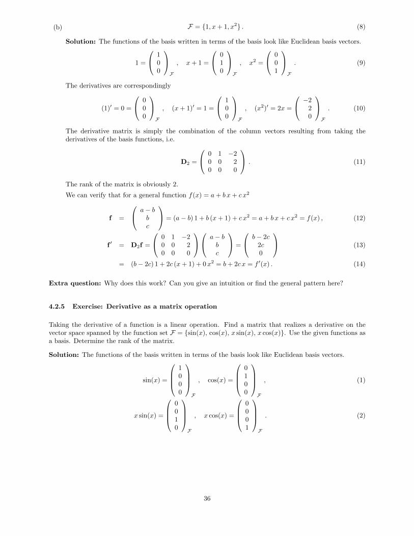
(b) F = {1, x+ 1, x2} . (8)


1 =

100

F

, x+ 1 =

010

F

, x2 =

001

F

. (9)


(1)′ = 0 =

000

F

, (x+ 1)′ = 1 =

100

F

, (x2)′ = 2x =

−220

F

. (10)


D2 =

0 1 −20 0 20 0 0

. (11)

The rank of the matrix is obviously 2.

We can verify that for a general function f(x) = a+ b x+ c x2

f =

a− bbc

= (a− b) 1 + b (x+ 1) + c x2 = a+ b x+ c x2 = f(x) , (12)

f ′ = D2f =

0 1 −20 0 20 0 0

a− bbc

=

b− 2c2c0

(13)

= (b− 2c) 1 + 2c (x+ 1) + 0x2 = b+ 2c x = f ′(x) . (14)

34

(c) F = {exp(x), exp(2x)} . (15)


exp(x) =

(10

)F, exp(2x) =

(01

)F. (16)


(exp(x))′ = exp(x) =

(10

)F, (exp(2x))′ = 2 exp(2x) =

(02

)F. (17)


D3 =

(1 00 2

). (18)

Interpreted as a transoformation the matrix performs a stretching along the second axis by a factor oftwo. The rank of the matrix is obviously 2.

We can verify that for a general function f(x) = a exp(x) + b exp(2x)

f =

(ab

)= a exp(x) + b exp(2x) = f(x) , (19)

f ′ = D3f =

(1 00 2

)(ab

)=

(a2b

)(20)

= a exp(x) + 2b exp(2x) = f ′(x) . (21)


Taking the derivative of a function is a linear operation. Find a matrix that realizes a derivative on thevector spaces spanned by the following function sets F . Use the given functions as a basis with respect towhich you represent the vectors. Determine the rank of each matrix.

(a) F = {sin(x), cos(x)} . (1)


sin(x) =

(10

)F, cos(x) =

(01

)F. (2)



(01

)F, (cos(x))′ = − sin(x) =

(−1

0

)F. (3)


D1 =

(0 −11 0

). (4)

Interpreted as a transformation the matrix performs a rotation by 90°. The rank of the matrix isobviously 2.

We can verify that for a general function f(x) = a sin(x) + b cos(x) considered as a vector f within thegiven vector space the derivative can actually be computed with D1.

f =

(ab

)= a sin(x) + b cos(x) = f(x) , (5)

f ′ = D1f =

(0 −11 0

)(ab

)=

(−ba

)(6)

= −b sin(x) + a cos(x) = a cos(x)− b sin(x) = f ′(x) . (7)

35

(b) F = {1, x+ 1, x2} . (8)


1 =

100

F

, x+ 1 =

010

F

, x2 =

001

F

. (9)


(1)′ = 0 =

000

F

, (x+ 1)′ = 1 =

100

F

, (x2)′ = 2x =

−220

F

. (10)


D2 =

0 1 −20 0 20 0 0

. (11)


We can verify that for a general function f(x) = a+ b x+ c x2

f =

a− bbc

= (a− b) 1 + b (x+ 1) + c x2 = a+ b x+ c x2 = f(x) , (12)

f ′ = D2f =

0 1 −20 0 20 0 0

a− bbc

=

b− 2c2c0

(13)

= (b− 2c) 1 + 2c (x+ 1) + 0x2 = b+ 2c x = f ′(x) . (14)

Extra question: Why does this work? Can you give an intuition or find the general pattern here?


Taking the derivative of a function is a linear operation. Find a matrix that realizes a derivative on thevector space spanned by the function set F = {sin(x), cos(x), x sin(x), x cos(x)}. Use the given functions asa basis. Determine the rank of the matrix.


sin(x) =

1000

F

, cos(x) =

0100

F

, (1)

x sin(x) =

0010

F

, x cos(x) =

0001

F

. (2)

36



0100

F

, (cos(x))′ = − sin(x) =

−1

000

F

, (3)

(x sin(x))′ = sin(x) + x cos(x) =

1001

F

, (x cos(x))′ = cos(x)− x sin(x) =

01−1

0

F

. (4)

The derivative matrix is simply the combination of the column vectors resulting from taking the derivativesof the basis functions, i.e.

D =

0 −1 1 01 0 0 10 0 0 −10 0 1 0

. (5)


4.3 Rank of a matrix

4.4 Determinant

4.4.1 Exercise: Determinants

Calculate the determinants of the following matrices.

(a)M1 =

(cos(φ) sin(φ)− sin(φ) cos(φ)

)(1)

Solution: The formula for the determinant of a 2× 2-matrix yields

|M1| = cos(φ) cos(φ)− (− sin(φ)) sin(φ) = 1 . (2)

This result is not surprising, since M1 is a rotation matrix, which obviously does not change the volumeof the unit square under its transformation.

(b)M2 =

1 2 30 1 2−1 0 1

(3)

Solution: We apply the formula for the determinant for 3× 3-matrices and obtain

|M1| = 1 · 1 · 1 + 2 · 2 · (−1) + 3 · 0 · 0− (−1) · 1 · 3− 0 · 2 · 1− 1 · 0 · 2 (4)

= 1− 4 + 0 + 3− 0− 0 = 0 . (5)

This indicates that the vectors of the matrix are linearly dependent. Indeed, two times the secondcolumn minus the third column equals the first column.

(c)

M3 =

1 1 1 0−1 1 1 0

0 0 1 10 1 0 0

(6)

37

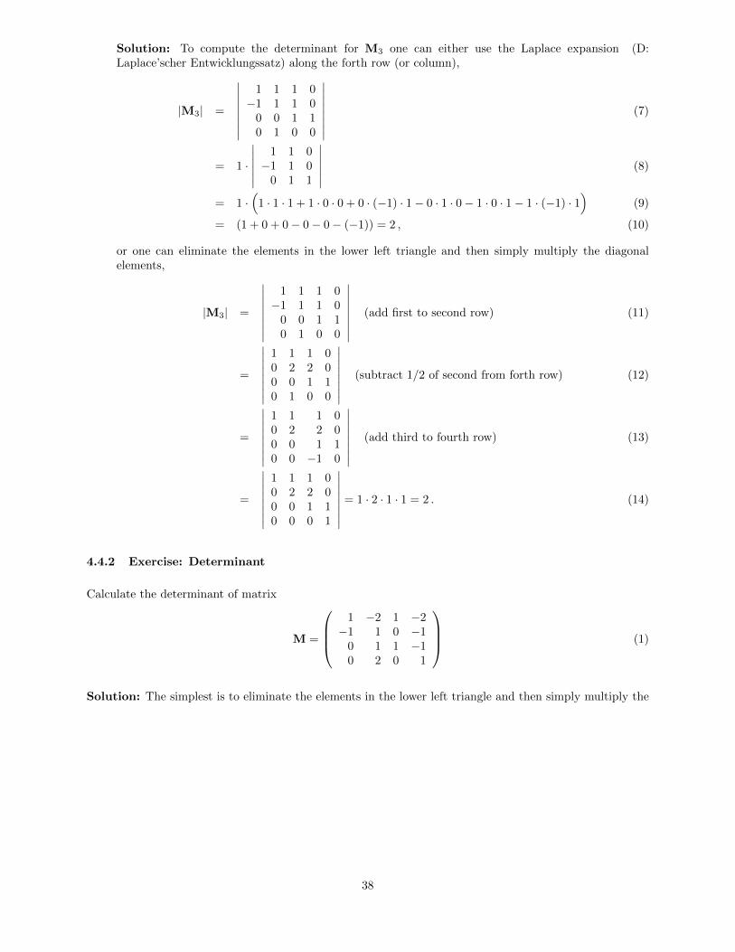
Solution: To compute the determinant for M3 one can either use the Laplace expansion (D:Laplace’scher Entwicklungssatz) along the forth row (or column),

|M3| =

∣∣∣∣∣∣∣∣1 1 1 0−1 1 1 0

0 0 1 10 1 0 0

∣∣∣∣∣∣∣∣ (7)

= 1 ·

∣∣∣∣∣∣1 1 0−1 1 0

0 1 1

∣∣∣∣∣∣ (8)

= 1 ·(

1 · 1 · 1 + 1 · 0 · 0 + 0 · (−1) · 1− 0 · 1 · 0− 1 · 0 · 1− 1 · (−1) · 1)

(9)

= (1 + 0 + 0− 0− 0− (−1)) = 2 , (10)

or one can eliminate the elements in the lower left triangle and then simply multiply the diagonalelements,

|M3| =

∣∣∣∣∣∣∣∣1 1 1 0−1 1 1 0

0 0 1 10 1 0 0

∣∣∣∣∣∣∣∣ (add first to second row) (11)

=

∣∣∣∣∣∣∣∣1 1 1 00 2 2 00 0 1 10 1 0 0

∣∣∣∣∣∣∣∣ (subtract 1/2 of second from forth row) (12)

=

∣∣∣∣∣∣∣∣1 1 1 00 2 2 00 0 1 10 0 −1 0

∣∣∣∣∣∣∣∣ (add third to fourth row) (13)

=

∣∣∣∣∣∣∣∣1 1 1 00 2 2 00 0 1 10 0 0 1

∣∣∣∣∣∣∣∣ = 1 · 2 · 1 · 1 = 2 . (14)

4.4.2 Exercise: Determinant

Calculate the determinant of matrix

M =

1 −2 1 −2−1 1 0 −1

0 1 1 −10 2 0 1

(1)

Solution: The simplest is to eliminate the elements in the lower left triangle and then simply multiply the

38

diagonal elements,

|M| =

∣∣∣∣∣∣∣∣1 −2 1 −2−1 1 0 −1

0 1 1 −10 2 0 1

∣∣∣∣∣∣∣∣ (add first to second row) (2)

=

∣∣∣∣∣∣∣∣1 −2 1 −20 −1 1 −30 1 1 −10 2 0 1

∣∣∣∣∣∣∣∣ (add second to third row and 2× second to fourth row) (3)

=

∣∣∣∣∣∣∣∣1 −2 1 −20 −1 1 −30 0 2 −40 0 2 −5

∣∣∣∣∣∣∣∣ (subtract third from fourth row) (4)

=

∣∣∣∣∣∣∣∣1 −2 1 −20 −1 1 −30 0 2 −40 0 0 −1

∣∣∣∣∣∣∣∣ = 1 · (−1) · 2 · (−1) = 2 . (5)

4.4.3 Exercise: Determinant

Calculate the determinant of matrix

M =

8 −2 1 7−3 −1 3 −3−4 0 2 −4−17 4 −2 −15

(1)

Solution: The simplest is to eliminate the elements in the lower left triangle and then simply multiply thediagonal elements,

|M| =

∣∣∣∣∣∣∣∣8 −2 1 7−3 −1 3 −3−4 0 2 −4−17 4 −2 −15

∣∣∣∣∣∣∣∣ (subtract fourth column from first column) (2)

=

∣∣∣∣∣∣∣∣1 −2 1 70 −1 3 −30 0 2 −4−2 4 −2 −15

∣∣∣∣∣∣∣∣ (add 2× first row to fourth row) (3)

=

∣∣∣∣∣∣∣∣1 −2 1 70 −1 3 −30 0 2 −40 0 0 −1

∣∣∣∣∣∣∣∣ = 1 · (−1) · 2 · (−1) = 2 . (4)

4.5 Inversion +

4.6 Trace

4.6.1 Exercise: Trace and determinant of a symmetric matrix

1. Show that the trace of a symmetric matrix equals the sum of its eigenvalues.

Solution: Let M be a symmetric square matrix. Since M is symmetric it can always be decomposedinto a product of its diagonal eigenvalue matrix Λ = diag(λ1, ..., λN ) and its orthogonal eigenvector

39

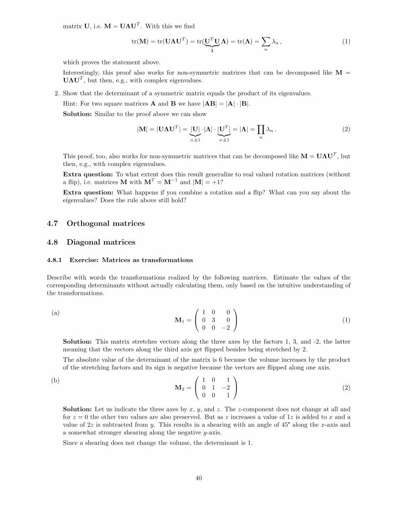
matrix U, i.e. M = UΛUT . With this we find

tr(M) = tr(UΛUT ) = tr(UTU︸︷︷︸1

Λ) = tr(Λ) =∑n

λn , (1)

which proves the statement above.

Interestingly, this proof also works for non-symmetric matrices that can be decomposed like M =UΛUT , but then, e.g., with complex eigenvalues.

2. Show that the determinant of a symmetric matrix equals the product of its eigenvalues.

Hint: For two square matrices A and B we have |AB| = |A| · |B|.Solution: Similar to the proof above we can show

|M| = |UΛUT | = |U|︸︷︷︸=±1

·|Λ| · |UT |︸︷︷︸=±1

= |Λ| =∏n

λn . (2)

This proof, too, also works for non-symmetric matrices that can be decomposed like M = UΛUT , butthen, e.g., with complex eigenvalues.

Extra question: To what extent does this result generalize to real valued rotation matrices (withouta flip), i.e. matrices M with MT = M−1 and |M| = +1?

Extra question: What happens if you combine a rotation and a flip? What can you say about theeigenvalues? Does the rule above still hold?

4.7 Orthogonal matrices

4.8 Diagonal matrices

4.8.1 Exercise: Matrices as transformations

Describe with words the transformations realized by the following matrices. Estimate the values of thecorresponding determinants without actually calculating them, only based on the intuitive understanding ofthe transformations.

(a)M1 =

1 0 00 3 00 0 −2

(1)

Solution: This matrix stretches vectors along the three axes by the factors 1, 3, and -2, the lattermeaning that the vectors along the third axis get flipped besides being stretched by 2.

The absolute value of the determinant of the matrix is 6 because the volume increases by the productof the stretching factors and its sign is negative because the vectors are flipped along one axis.

(b)M2 =

1 0 10 1 −20 0 1

(2)

Solution: Let us indicate the three axes by x, y, and z. The z-component does not change at all andfor z = 0 the other two values are also preserved. But as z increases a value of 1z is added to x and avalue of 2z is subtracted from y. This results in a shearing with an angle of 45° along the x-axis anda somewhat stronger shearing along the negative y-axis.

Since a shearing does not change the volume, the determinant is 1.

40

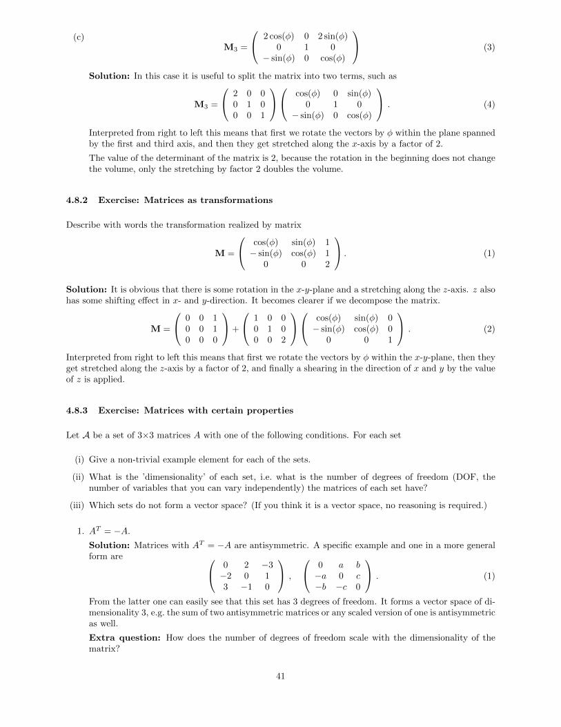
(c)M3 =

2 cos(φ) 0 2 sin(φ)0 1 0

− sin(φ) 0 cos(φ)

(3)

Solution: In this case it is useful to split the matrix into two terms, such as

M3 =

2 0 00 1 00 0 1

cos(φ) 0 sin(φ)0 1 0

− sin(φ) 0 cos(φ)

. (4)

Interpreted from right to left this means that first we rotate the vectors by φ within the plane spannedby the first and third axis, and then they get stretched along the x-axis by a factor of 2.

The value of the determinant of the matrix is 2, because the rotation in the beginning does not changethe volume, only the stretching by factor 2 doubles the volume.

4.8.2 Exercise: Matrices as transformations

Describe with words the transformation realized by matrix

M =

cos(φ) sin(φ) 1− sin(φ) cos(φ) 1

0 0 2

. (1)

Solution: It is obvious that there is some rotation in the x-y-plane and a stretching along the z-axis. z alsohas some shifting effect in x- and y-direction. It becomes clearer if we decompose the matrix.

M =

0 0 10 0 10 0 0

+

1 0 00 1 00 0 2

cos(φ) sin(φ) 0− sin(φ) cos(φ) 0

0 0 1

. (2)

Interpreted from right to left this means that first we rotate the vectors by φ within the x-y-plane, then theyget stretched along the z-axis by a factor of 2, and finally a shearing in the direction of x and y by the valueof z is applied.

4.8.3 Exercise: Matrices with certain properties

Let A be a set of 3×3 matrices A with one of the following conditions. For each set

(i) Give a non-trivial example element for each of the sets.

(ii) What is the ’dimensionality’ of each set, i.e. what is the number of degrees of freedom (DOF, thenumber of variables that you can vary independently) the matrices of each set have?

(iii) Which sets do not form a vector space? (If you think it is a vector space, no reasoning is required.)

1. AT = −A.

Solution: Matrices with AT = −A are antisymmetric. A specific example and one in a more generalform are 0 2 −3

−2 0 13 −1 0

,

0 a b−a 0 c−b −c 0

. (1)

From the latter one can easily see that this set has 3 degrees of freedom. It forms a vector space of di-mensionality 3, e.g. the sum of two antisymmetric matrices or any scaled version of one is antisymmetricas well.

Extra question: How does the number of degrees of freedom scale with the dimensionality of thematrix?

41

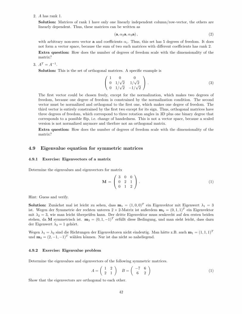
2. A has rank 1.

Solution: Matrices of rank 1 have only one linearly independent column/row-vector, the others arelinearly dependent. Thus, these matrices can be written as

(a, α2a, α3a) , (2)

with arbitrary non-zero vector a and coefficients αi. Thus, this set has 5 degrees of freedom. It doesnot form a vector space, because the sum of two such matrices with different coefficients has rank 2.


3. AT = A−1.

Solution: This is the set of orthogonal matrices. A specific example is 1 0 0

0 1/√

2 1/√

2

0 1/√

2 −1/√

2

. (3)

The first vector could be chosen freely, except for the normalization, which makes two degrees offreedom, because one degree of freedom is constrained by the normalization condition. The secondvector must be normalized and orthogonal to the first one, which makes one degree of freedom. Thethird vector is entirely constrained by the first two except for its sign. Thus, orthogonal matrices havethree degrees of freedom, which correspond to three rotation angles in 3D plus one binary degree thatcorresponds to a possible flip, i.e. change of handedness. This is not a vector space, because a scaledversion is not normalized anymore and therfore not an orthogonal matrix.


4.9 Eigenvalue equation for symmetric matrices

4.9.1 Exercise: Eigenvectors of a matrix

Determine the eigenvalues and eigenvectors for matrix

M =

3 0 00 2 10 1 2

. (1)

Hint: Guess and verify.

Solution: Zunachst mal ist leicht zu sehen, dass m1 = (1, 0, 0)T ein Eigenvektor mit Eigenwert λ1 = 3ist. Wegen der Symmetrie der rechten unteren 2 × 2-Matrix ist außerdem m2 = (0, 1, 1)T ein Eigenvektormit λ2 = 3, wie man leicht uberprufen kann. Der dritte Eigenvektor muss senkrecht auf den ersten beidenstehen, da M symmetrisch ist. m3 = (0, 1,−1)T erfullt diese Bedingung, und man sieht leicht, dass dazuder Eigenwert λ3 = 1 gehort.

Wegen λ1 = λ2 sind die Richtungen der Eigenvektoren nicht eindeutig. Man hatte z.B. auch m1 = (1, 1, 1)T

und m2 = (2,−1,−1)T wahlen konnen. Nur ist das nicht so naheliegend.

4.9.2 Exercise: Eigenvalue problem

Determine the eigenvalues and eigenvectors of the following symmetric matrices.

A =

(1 22 1

)B =

(−7 66 2

)(1)

Show that the eigenvectors are orthogonal to each other.

42

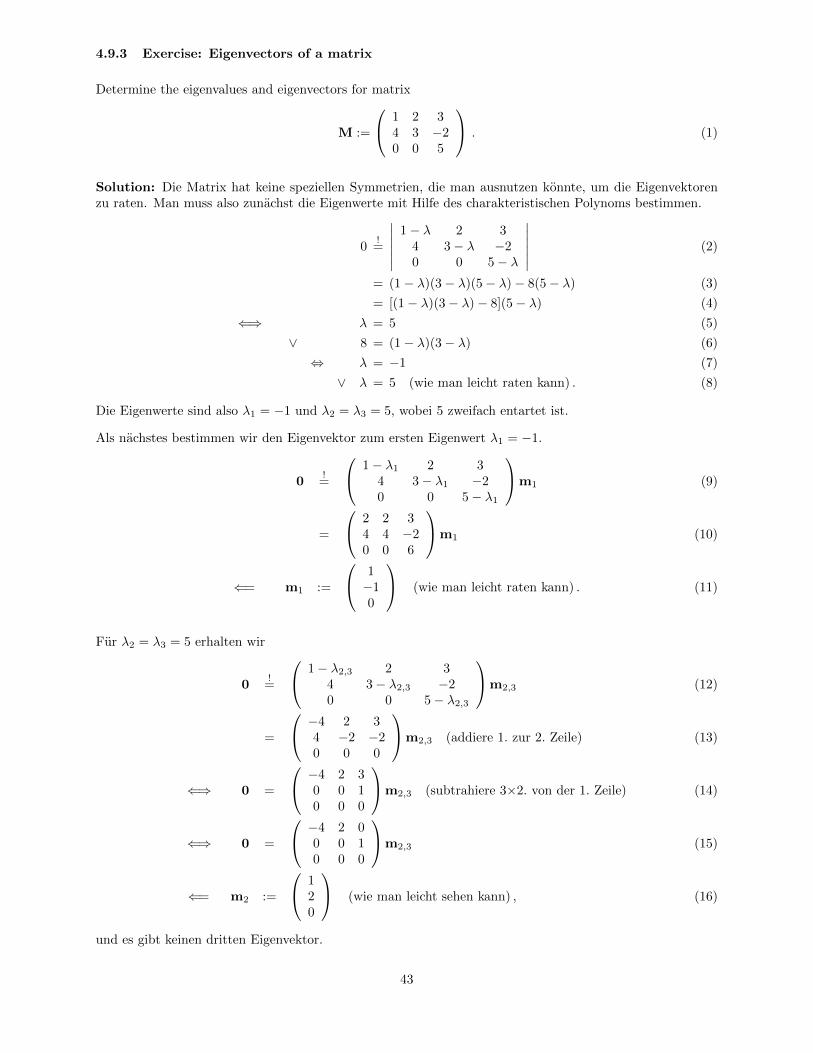
4.9.3 Exercise: Eigenvectors of a matrix

Determine the eigenvalues and eigenvectors for matrix

M :=

1 2 34 3 −20 0 5

. (1)

Solution: Die Matrix hat keine speziellen Symmetrien, die man ausnutzen konnte, um die Eigenvektorenzu raten. Man muss also zunachst die Eigenwerte mit Hilfe des charakteristischen Polynoms bestimmen.

0!=

∣∣∣∣∣∣1− λ 2 3

4 3− λ −20 0 5− λ

∣∣∣∣∣∣ (2)

= (1− λ)(3− λ)(5− λ)− 8(5− λ) (3)

= [(1− λ)(3− λ)− 8](5− λ) (4)

⇐⇒ λ = 5 (5)

∨ 8 = (1− λ)(3− λ) (6)

⇔ λ = −1 (7)

∨ λ = 5 (wie man leicht raten kann) . (8)

Die Eigenwerte sind also λ1 = −1 und λ2 = λ3 = 5, wobei 5 zweifach entartet ist.

Als nachstes bestimmen wir den Eigenvektor zum ersten Eigenwert λ1 = −1.

0!=

1− λ1 2 34 3− λ1 −20 0 5− λ1

m1 (9)

=

2 2 34 4 −20 0 6

m1 (10)

⇐= m1 :=

1−10

(wie man leicht raten kann) . (11)

Fur λ2 = λ3 = 5 erhalten wir

0!=

1− λ2,3 2 34 3− λ2,3 −20 0 5− λ2,3

m2,3 (12)

=

−4 2 34 −2 −20 0 0

m2,3 (addiere 1. zur 2. Zeile) (13)

⇐⇒ 0 =

−4 2 30 0 10 0 0

m2,3 (subtrahiere 3×2. von der 1. Zeile) (14)

⇐⇒ 0 =

−4 2 00 0 10 0 0

m2,3 (15)

⇐= m2 :=

120

(wie man leicht sehen kann) , (16)

und es gibt keinen dritten Eigenvektor.

43

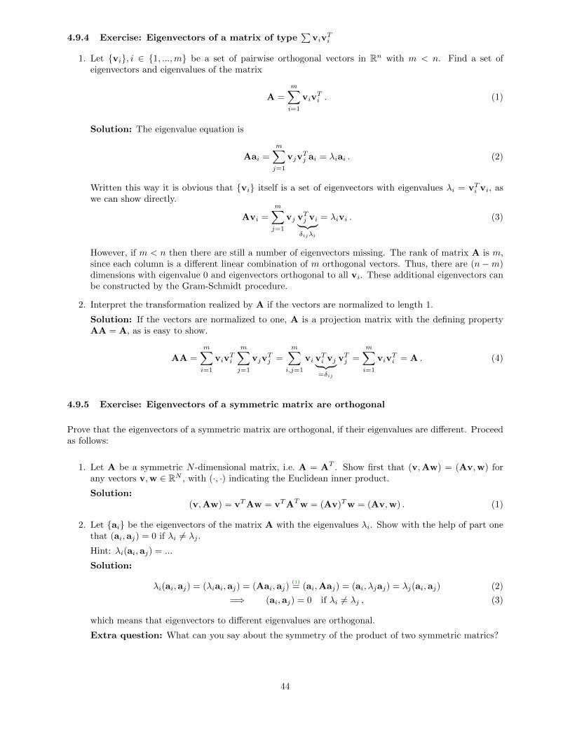
4.9.4 Exercise: Eigenvectors of a matrix of type∑

vivTi

1. Let {vi}, i ∈ {1, ...,m} be a set of pairwise orthogonal vectors in Rn with m < n. Find a set ofeigenvectors and eigenvalues of the matrix

A =

m∑i=1

vivTi . (1)

Solution: The eigenvalue equation is

Aai =

m∑j=1

vjvTj ai = λiai . (2)

Written this way it is obvious that {vi} itself is a set of eigenvectors with eigenvalues λi = vTi vi, aswe can show directly.

Avi =

m∑j=1

vj vTj vi︸︷︷︸δijλi

= λivi . (3)

However, if m < n then there are still a number of eigenvectors missing. The rank of matrix A is m,since each column is a different linear combination of m orthogonal vectors. Thus, there are (n −m)dimensions with eigenvalue 0 and eigenvectors orthogonal to all vi. These additional eigenvectors canbe constructed by the Gram-Schmidt procedure.

2. Interpret the transformation realized by A if the vectors are normalized to length 1.

Solution: If the vectors are normalized to one, A is a projection matrix with the defining propertyAA = A, as is easy to show.

AA =

m∑i=1

vivTi

m∑j=1

vjvTj =

m∑i,j=1

vi vTi vj︸︷︷︸=δij

vTj =

m∑i=1

vivTi = A . (4)

4.9.5 Exercise: Eigenvectors of a symmetric matrix are orthogonal

Prove that the eigenvectors of a symmetric matrix are orthogonal, if their eigenvalues are different. Proceedas follows:

1. Let A be a symmetric N -dimensional matrix, i.e. A = AT . Show first that (v,Aw) = (Av,w) forany vectors v,w ∈ RN , with (·, ·) indicating the Euclidean inner product.

Solution:(v,Aw) = vTAw = vTATw = (Av)Tw = (Av,w) . (1)

2. Let {ai} be the eigenvectors of the matrix A with the eigenvalues λi. Show with the help of part onethat (ai,aj) = 0 if λi 6= λj .

Hint: λi(ai,aj) = ...

Solution:

λi(ai,aj) = (λiai,aj) = (Aai,aj)(1)= (ai,Aaj) = (ai, λjaj) = λj(ai,aj) (2)

=⇒ (ai,aj) = 0 if λi 6= λj , (3)

which means that eigenvectors to different eigenvalues are orthogonal.

Extra question: What can you say about the symmetry of the product of two symmetric matrics?

44

4.10 General eigenvectors

4.10.1 Exercise: Matrices with given eigenvectors and -values

1. Construct a matrix M that has the following right-eigenvectors ri (not normalized!) and eigenvaluesλi.

r1 = (1, 0)T , λ1 = 1 , r2 = (1, 1)T , λ2 = 2 . (1)

Verify your result.

Solution: To construct a matrix with the given right-eigenvectors, one can first construct a set of

left-eigenvectors li that are orthogonal to the other right-eigenvectors, i.e. a set with lT

i rj = 0 for j 6= i.It is easy to see that

l1 := (−1, 1)T , l2 := (0, 1)T (2)

fulfill this requirement. Next we scale the left-eigenvectors such that the inner products lTi ri equal theeigenvalues λi. Thus,

l1 := l1/(lT

1 r1

)· λ1 = (−1, 1)T /(−1) · 1 = (1,−1)T , (3)

l2 := l2/(lT

2 r2

)· λ2 = (0, 1)T /1 · 2 = (0, 2)T . (4)

With these scaled left-eigenvectors, we can construct matrix M.

M := r1lT1 + r2l

T2 =

(10

)(1,−1) +

(11

)(0, 2) (5)

=

(1 −10 0

)+

(0 20 2

)=

(1 10 2

). (6)

One could have seen this in this concrete case also more directly as follows (Kai Brugge, SS’09). AsM(1, 0)T = (1, 0)T the first column of M must be (1, 0)T , because the second column does not playany role in the product with (1, 0)T . As M(1, 1)T = (2, 2)T the second column of the matrix mustthen be (1, 2)T to make the sum of the two columns equal to (2, 2)T .

We verify that the ri are indeed right-eigenvectors to the eigenvalues λi.

Mr1 =

(1 10 2

)(10

)=

(10

)= 1

(10

)= λ1r1 , (7)

Mr2 =

(1 10 2

)(11

)=

(22

)= 2

(11

)= λ1r2 . (8)

2. Determine the left-eigenvectors and the corresponding eigenvalues of matrix M. Verify your result.

Solution: On the way of constructing the matrix we have constructed also the left-eigenvectors already.The eigenvalues should be the same as for the right-eigenvectors, because

lTi M = lTi (r1lT1 + r2l

T2 ) = lTi r1︸︷︷︸

=δi1λ1

lT1 + lTi r2︸︷︷︸=δi2λ2

lT2 = λilTi . (9)

For the concrete matrix above we verify that

lT1 M = (1,−1)

(1 10 2

)= (1,−1) = 1(1,−1) = λ1l

T1 , (10)

lT2 M = (0, 2)

(1 10 2

)= (0, 4) = 2(0, 2) = λ2l

T2 . (11)

If one has chosen the more direct way in the first part, one has to work harder here and determine theleft-eigenvectors and the corresponding eigenvalues the normal way.

Extra question: What can you say about the eigenvalues of an upper triangular matrix?

45

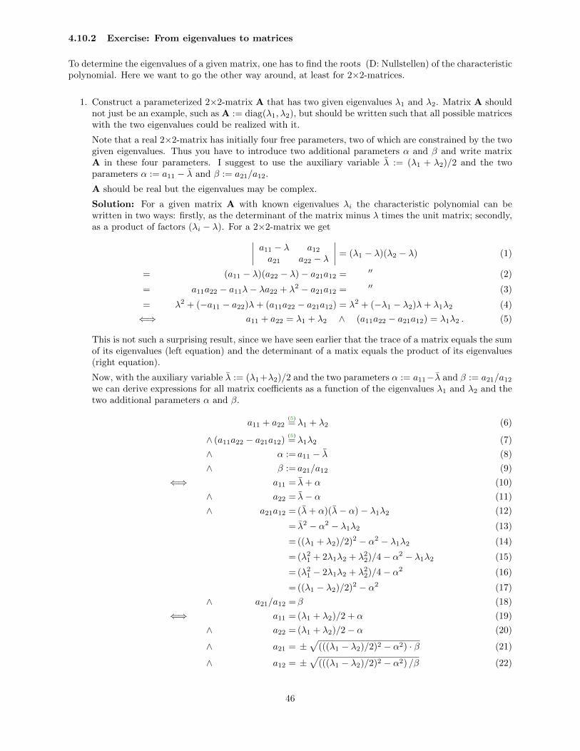
4.10.2 Exercise: From eigenvalues to matrices

To determine the eigenvalues of a given matrix, one has to find the roots (D: Nullstellen) of the characteristicpolynomial. Here we want to go the other way around, at least for 2×2-matrices.

1. Construct a parameterized 2×2-matrix A that has two given eigenvalues λ1 and λ2. Matrix A shouldnot just be an example, such as A := diag(λ1, λ2), but should be written such that all possible matriceswith the two eigenvalues could be realized with it.

Note that a real 2×2-matrix has initially four free parameters, two of which are constrained by the twogiven eigenvalues. Thus you have to introduce two additional parameters α and β and write matrixA in these four parameters. I suggest to use the auxiliary variable λ := (λ1 + λ2)/2 and the twoparameters α := a11 − λ and β := a21/a12.

A should be real but the eigenvalues may be complex.

Solution: For a given matrix A with known eigenvalues λi the characteristic polynomial can bewritten in two ways: firstly, as the determinant of the matrix minus λ times the unit matrix; secondly,as a product of factors (λi − λ). For a 2×2-matrix we get∣∣∣∣ a11 − λ a12

a21 a22 − λ

∣∣∣∣ = (λ1 − λ)(λ2 − λ) (1)

= (a11 − λ)(a22 − λ)− a21a12 = ′′ (2)

= a11a22 − a11λ− λa22 + λ2 − a21a12 = ′′ (3)

= λ2 + (−a11 − a22)λ+ (a11a22 − a21a12) = λ2 + (−λ1 − λ2)λ+ λ1λ2 (4)

⇐⇒ a11 + a22 = λ1 + λ2 ∧ (a11a22 − a21a12) = λ1λ2 . (5)

This is not such a surprising result, since we have seen earlier that the trace of a matrix equals the sumof its eigenvalues (left equation) and the determinant of a matix equals the product of its eigenvalues(right equation).

Now, with the auxiliary variable λ := (λ1+λ2)/2 and the two parameters α := a11−λ and β := a21/a12we can derive expressions for all matrix coefficients as a function of the eigenvalues λ1 and λ2 and thetwo additional parameters α and β.

a11 + a22(5)= λ1 + λ2 (6)

∧ (a11a22 − a21a12)(5)= λ1λ2 (7)

∧ α := a11 − λ (8)

∧ β := a21/a12 (9)

⇐⇒ a11 = λ+ α (10)

∧ a22 = λ− α (11)

∧ a21a12 = (λ+ α)(λ− α)− λ1λ2 (12)

= λ2 − α2 − λ1λ2 (13)

= ((λ1 + λ2)/2)2 − α2 − λ1λ2 (14)

= (λ21 + 2λ1λ2 + λ22)/4− α2 − λ1λ2 (15)

= (λ21 − 2λ1λ2 + λ22)/4− α2 (16)

= ((λ1 − λ2)/2)2 − α2 (17)

∧ a21/a12 =β (18)

⇐⇒ a11 = (λ1 + λ2)/2 + α (19)

∧ a22 = (λ1 + λ2)/2− α (20)

∧ a21 = ±√

(((λ1 − λ2)/2)2 − α2) · β (21)

∧ a12 = ±√

(((λ1 − λ2)/2)2 − α2) /β (22)

46

⇐⇒ A =

((λ1 + λ2)/2 + α ±

√(((λ1 − λ2)/2)2 − α2) /β

±√

(((λ1 − λ2)/2)2 − α2) · β (λ1 + λ2)/2− α

). (23)

Note that the ± have to be chosen consistently, either both ’+’ or both ’−’. Furthermore, the conditionthat A is real leads to the constraint that

0 ≤ ((λ1 − λ2)/2)2 − α2 (24)

⇐⇒ |α| ≤ |(λ1 − λ2)/2| . (25)

2. Interpret the result. What happens with the eigenvectors if you set β = 0 and vary α? What happensif you set α = 0 and vary β?

Solution: To understand the structure of matrix A as written in (23) first consider the case of β = 1.In that case matrix A is symmetric and its eigenvalues must be orthogonal. Since the eigenvalues aregiven by λ1 and λ2, the only freedom left is the overall orientation of the eigenvectors, which must bedetermined by α. For instance, if α assumes one of the extreme values α = ±(λ1 − λ2)/2 permittedby (25), matrix A becomes A = diag(λ1, λ2) (for ’+’) or A = diag(λ2, λ1) (for ’−’) and the eigenvectorsare aligned with the coordinate axes. If α = 0 then

A =

((λ1 + λ2)/2 ±(λ1 − λ2)/2±(λ1 − λ2)/2 (λ1 + λ2)/2

)(26)

and the eigenvectors are rotated by 45◦, as can be easily checked for ’+’.((λ1 + λ2)/2 +(λ1 − λ2)/2

+(λ1 − λ2)/2 (λ1 + λ2)/2

)(11

)= λ1

(11

), (27)(

(λ1 + λ2)/2 +(λ1 − λ2)/2+(λ1 − λ2)/2 (λ1 + λ2)/2

)(1−1

)= λ2

(1−1

). (28)

For ’−’ the eigenvectors would be the same but the eigenvalues would be exchanges.

Parameter β only plays a role if α does not assume one of the extreme values α = ±(λ1−λ2)/2. In thatcase β 6= 0 makes the matrix asymmetric, which leads to non-orthogonal eigenvectors. For instancewith α = 0, λ1 = 3 and λ2 = 1 we get

A =

(2 ±

√1/β

±√β 2

), (29)

and the eigenvalue equations for ’+’ become(2

√1/β√

β 2

)(x1y1

)= 3

(x1y1

)(30)

⇐⇒ 2x1 +√

1/β y1 = 3x1 (31)

∧√β x1 + 2y1 = 3y1 (32)

⇐⇒√

1/β y1 = x1 (33)

∧√β x1 = y1 (34)

⇐=

(x1y1

)=

(1√β

)(35)

and (2

√1/β√

β 2

)(x1y1

)= 1

(x1y1

)(36)

⇐⇒ 2x1 +√

1/β y1 = x1 (37)

∧√β x1 + 2y1 = y1 (38)

⇐⇒√

1/β y1 = −x1 (39)

∧√β x1 = −y1 (40)

⇐=

(x1y1

)=

(1−√β

). (41)

47

β = 1 yields the eigenvectors from above, see (27, 28). For larger values of β the eigenvectors turnmore away from the abscissa, and for smaller values the eigenvectors turn more together.

4.10.3 Exercise: Generalized eigenvalue problem

Consider the generalized eigenvalue problem

Aui = λiBui (1)

with some real N × N matrices A and B. The λi are the right-eigenvalues and the ui are the (non-zero)right-eigenvectors. To find corresponding left-eigenvalues µ and left-eigenvectors vi, one has to solve theequation

vTi A = µivTi B (2)

1. Show that left- and right-eigenvalues are identical.

Solution: For the right-eigenvalues we find the condition that

Aui(1)= λiBui (3)

⇐⇒ (A− λiB)ui = 0 (4)

=⇒ |A− λiB| = 0 (5)

For the left-eigenvalues we find analogously

vTi A(2)= µiv

Ti B (6)

⇐⇒ vTi (A− µiB) = 0T (7)

=⇒ |A− µiB| = 0 (8)

Since the conditions for λi and µi are identical, the left- and right-eigenvalues are identical and aresimply called eigenvalues λi.

2. Show that vTj Aui = 0 as well as vTj Bui = 0 for λi 6= λj .

Hint: Consider (1) and (2) simultaneously with different eigenvalues.

Solution: We consider the right- and left-eigenvalue equation for i and j, respectively,

Aui(1)= λiBui |vTj · (9)

∧ vTj A(2)= λjv

Tj B | · ui (10)

=⇒ vTj Aui = λivTj Bui (11)

∧ vTj Aui = λjvTj Bui (12)

⇐⇒ vTj Aui = 0 (13)

∧ vTj Bui = 0 (since λi 6= λj) (14)

Notice that this is even true if either λi = 0 or λj = 0, but not both, of course.

3. Show that for symmetric A and B the right-eigenvectors are also left-eigenvectors.

Solution: This is easy to see if we transpose the right-eigenvalue equation.

Aui(1)= λiBui |·T (15)

⇐⇒ uTi AT = λiuTi BT (16)

⇐⇒ uTi A = λiuTi B (since A = AT and B = BT ) (17)

⇐⇒ (2) (18)

Thus, right-eigenvectors are also left-eigenvectors and we can simply speak of eigenvectors.

48

4. Show that for symmetric A and B we have uTj Aui = 0 as well as uTj Bui = 0 for λi 6= λj .

Solution: This follows trivially from the last two points of this exercise. This is not generally true fornon-symmetric matrices.

5. For symmetric A and B it is convenient to normalize the eigenvectors such that uTi Bui = 1. Assumethe eigenvectors form a basis, i.e. they are complete, and you want to represent an arbitrary vector ywrt this basis, i.e.

y =∑i

αiui (19)

Which constraint on the αi follows from the constraint yTBy = 1?

Solution:

1!= yTBy (20)

=∑i,j

αiαj uTi Buj︸︷︷︸= δij

(21)

=∑i

α2i (22)

6. Assume A and B are symmetric and you want to minimize (or maiximze) yTAy under the constraintyTBy = 1. What is the solution?

Hint: Use ansatz (19) and assume uTi Bui = 1.

Solution: We want to minimize (or maximize)

yTAy(19)=∑i,j

αiαjuTi Auj (23)

(1)=∑i,j

αiαjλjuTi uTi Buj︸︷︷︸

= δij

(24)

=∑i

α2iλi (25)

Since this is minimized (or maximized) subject to∑i α

2i = 1 it is quite obvious that αi = δ1i is an

optimal solution if the eigenvalues are ordered like λ1 ≤ λ2 ≤ ... ≤ λ1 (or λ1 ≥ λ2 ≥ ... ≥ λ1). Thusu1 is the optimal solution.

Extra question: If for some reason u1 is not wanted as a solution and the solution should be

orthogonal to it wrt a metric induced by B, i.e. yBu1!= 0, what would then be the optimal solution?

4.11 Complex eigenvalues

4.11.1 Exercise: Complex eigenvalues

Determine the (complex) eigenvalues and eigenvectors of the rotation matrix

D(φ) =

(cosφ sinφ− sinφ cosφ

). (1)

Solution: To find the eigenvalues λ of a matrix A one has to find the roots of the characteristic polynomial

49

det(A− λI).

0 =

∣∣∣∣ cosφ− λ sinφ− sinφ cosφ− λ

∣∣∣∣ (2)

= (cosφ− λ)(cosφ− λ)− (sinφ)(− sinφ) (3)

= (cosφ− λ)2 + sin2 φ (4)

⇐⇒ (λ− cosφ)2 = − sin2 φ (5)

⇐⇒ λ = cosφ±√− sin2 φ (6)

= cosφ± i

√sin2 φ (7)

= cosφ± i sinφ (could also be ∓ depending on φ) (8)

= e±iφ (Euler’s formula) . (9)

The first eigenvector is found by substituting the first eigenvalue, λ1, back into the eigenvalue equation.

Ax = λ1x (10)

⇐⇒(

cosφ sinφ− sinφ cosφ

)(x1x2

)= (cosφ+ i sinφ)

(x1x2

)(11)

⇐⇒ cos(φ)x1 + sin(φ)x2 = (cosφ+ i sinφ)x1 (12)

∧ − sin(φ)x1 + cos(φ)x2 = (cosφ+ i sinφ)x2 (13)

⇐⇒ sin(φ)x2 = i sin(φ)x1 (14)

∧ − sin(φ)x1 = i sin(φ)x2 (15)

⇐⇒ x2 = ix1 (if sin(φ) 6= 0) (16)

⇐= x1 =

(1i

). (17)

Similarly the second eigenvector (1,−i) can be derived, which is the complex conjugate of the first one, as wewould expect, since for real matrices, eigenvectors to complex eigenvalues always come in complex conjugatepairs.

Note also that, since we are in the complex domain, (i,−1)T = i(1, i)T is also an eigenvector if (1, i)T is one.

4.12 Nonquadratic matrices +

4.13 Quadratic forms +

50

Solutions to the Exercises Linear Algebra · Solutions to the Exercises* on Linear Algebra Laurenz...

Documents

Transcript of Solutions to the Exercises Linear Algebra · Solutions to the Exercises* on Linear Algebra Laurenz...