Solution of Algebraic Lyapunov Equation on Positive … [email protected] 2Department...

Copyright c© 2018 Tech Science Press CMC, vol.54, no.2, pp.181-195, 2018

Solution of Algebraic Lyapunov Equation on Positive-DefiniteHermitian Matrices by Using Extended Hamiltonian Algorithm

Muhammad Shoaib Arif 1, Mairaj Bibi 2 and Adnan Jhangir 3

Abstract: This communique is opted to study the approximate solution of the AlgebraicLyapunov equation on the manifold of positive-definite Hermitian matrices. We choosethe geodesic distance between −AHX −XA and P as the cost function, and put forwardthe Extended Hamiltonian algorithm (EHA) and Natural gradient algorithm (NGA) for thesolution. Finally, several numerical experiments give you an idea about the effectivenessof the proposed algorithms. We also show the comparison between these two algorithmsEHA and NGA. Obtained results are provided and analyzed graphically. We also concludethat the extended Hamiltonian algorithm has better convergence speed than the natural gra-dient algorithm, whereas the trajectory of the solution matrix is optimal in case of Naturalgradient algorithm (NGA) as compared to Extended Hamiltonian Algorithm (EHA). Theaim of this paper is to show that the Extended Hamiltonian algorithm (EHA) has superiorconvergence properties as compared to Natural gradient algorithm (NGA). Upto the best ofauthor’s knowledge, no approximate solution of the Algebraic Lyapunov equation on themanifold of positive-definite Hermitian matrices is found so far in the literature.

Keywords: Information geometry, algebraic lyapunov equation, positive-definite hermitianmatrix manifold, natural gradient algorithm, extended hamiltonian algorithm.

1 IntroductionIt is well known that many engineering and mathematical problems, say, signal processing,robot control and computer image processing [Cafaro (2008); Cohn and Parrish (1991);Barbaresco (2009); Brown and Harris (1994)], can be reduced as obtaining the numericalsolution of the following algebraic Lyapunov equation

AHX +XA+ P = 0, (1)

where P is a positive-definite Hermitian matrix, H denotes the conjugate transpose of aHermitian matrix.The solution of the algebraic Lyapunov equation is gaining more and more attention inthe field of computational mathematics [Datta (2004); Golub, Nash and Vanloan (1979)].Several algorithms are used to get the approximate solution of the above-mentioned e-quation. For instance, Ran et al. [Ran and Reurings (2004)] put forward the fixed point

1 Department of Mathematics, Air University, PAF Complex, E-9, Islamabad, Pakistan. E-mail: [email protected]

2 Department of Mathematics, Comsats Institute of Information Technology, Park Road, Chak-Shahzad, Islamabad, Pakistan. E-mail: [email protected]

3 Department of Mathematics, Comsats Institute of Information Technology, Wah Cantt, Pakistan.

CMC.doi:10.3970/cmc.2018.054.181 www.techscience.com/cmc

* Corresponding Author: Adnan Jhangir. Email: [email protected].

182 Copyright c© 2018 Tech Science Press CMC, vol.54, no.2, pp.181-195, 2018

algorithm, the Cholesky decomposition algorithm was presented by Li et al. [Li and White (2002)], and a preconditioned Krylov method to get the solution of the Lyapunov equation was given by Jbilou [Jbilou (2010)]. Vandereycken et al. [Vandereycken and Vandewalle (2010)] provided a Riemannian optimization approach to compute the low-rank solution of the Lyapunov matrix equation. Deng et al. [Deng, Bai and Gao (2006)] designed iterative orthogonal direction methods according to the fundamental idea of the classical conjugate direction method for the standard system of linear equations to obtain the Hermitian solu-tions of the linear matrix equations AXB = C and (AX, XB) = (C, D). Recently, Su et al. [Su and Chen (2010)] proposed a modified conjugate gradient algorithm (MCGA) to solve Lyapunov matrix equations and some other linear matrix equations, which seemed to be the generalized results. The traditional method like modified conjugate gradient algo-rithm (MCGA) are first order learning algorithms, hence the convergence speed of MCGA is very slow.Another interesting approach to solve algebraic Lyapunov equation is by considering the set of matrices as a manifold and applying the techniques from differential geometry and information geometry. Recently Arif et al. [Arif, Zhang and Sun (2016)] solved the alge-braic Lyapunov equation on matrix manifold by information geometric algorithm. Duan et al. [Duan, Sun and Zhang (2014); Duan, Sun, Peng et al. (2013)] solved continuous algebraic Lyapunov equation and discrete Lyapunov equation on the space of positive-definite symmetric matrices by using natural gradient algorithm. Also, Luo et al. [Luo and Sun (2014)] gives the solution of discrete algebraic Lyapunov equation on the space of positive-definite symmetric matrices by using Extended Hamiltonian algorithm. In both the papers, the authors have considered the set of positive-definite symmetric matrices as a matrix manifold and used the geodesic distance between AHX + XA and −P to find the solution matrix X .Up to date, however, there has been few investigation on the solution problem of the Lya-punov matrix equation in the view of Riemannian manifolds. Chein [Chein (2014)] gives the numerical solution of ill posed positive linear system he combines the methods from manifold theory and sliding mode control theory and develop an affine nonlinear dynami-cal system. This system is proven asymptotically stable by using argument from Lyapunov stability theory.In this article, a new frame work is proposed to calculate the numerical solution of con-tinuous algebraic Lyapunov matrix equation on the space of positive-definite Hermitian matrices by using natural gradient algorithm and Extended Hamiltonian algorithm. More-over, we present the comparison of the solution obtained by the two algorithms.Note that this solution is a positive definite Hermitian matrices is a global asymptotically stable linear system and the set of all the positive definite Hermitian matrices can be taken as a manifold. Thus, it is more convenient to investigate the solution problem with the help of these attractive features on the manifold. To address such a need, we focus on a numerical method to solve the Lyapunov matrix equation on the manifold.The gradient is usually adapted to minimize the cost function by adjusting the parameters of the manifold. However, the convergence speed can be seen to be slow if a small change in the parameters changes largely the cost function. In order to overcome this problem of poor convergence, the work has been done in two different directions. Firstly, Amari et al.[Amari (1998); Amari and Douglas (2000); Amari (1999)] introduced the Natural Gradi-

Solution of Algebraic Lyapunov Equation 183

ent Algorithm (NGA) which employed the Fisher information matrix on the Riemannian structure of manifold based on differential geometry. Another approach is based on the inclusion of momentum term in the ordinary gradient method to enhance the convergence speed. This is a second-order learning algorithm that was developed by Fiori et al. [Fiori (2011, 2012)], which is called the Extended Hamiltonian Algorithm (EHA).Although, both the natural gradient algorithm and extended Hamiltonian algorithm defines the steepest descent direction, but we must compute explicitly the Fisher information ma-trix in the natural gradient algorithm and the steepest descent direction in the extended Hamiltonian algorithm at each iterative step. So the computational cost of both the algo-rithms are comparatively high. Moreover, the trajectory of the parameters obtained by the implementation of extended Hamiltonian algorithm is closer to the geodesic as compared to one obtained by natural gradient algorithm.Rest of the paper is organized as follows. Section 2 is a preliminary survey on the mani-folds of positive-definite Hermitian m atrices. Third section presents the solution of alge-braic Lyapunov matrix equation by Extended Hamiltonian algorithm and Natural gradient algorithm and also illustrates the convergence speed of EHA compared with NGA using numerical examples. Section 4 concludes the results presented in section 3.

2 The Riemannian structure on the manifold of positive-definite Hermitian matricesIn this paper, we denote the set of n×n Positive-definite Hermitian matrices by H (n). This set can be considered as a Riemannian manifold by defining the Riemannian metric on it. Moakher [Moakher (2005)] in his paper, gives the concept of geodesic connecting two matrices on H(n). Observing that the geodesic distance represents the infimum of lengths of the curves connecting any two matrices. Here, we take geodesic distance as the cost function to minimize the distance between two matrices in H(n). The following background material and important results are taken from Zhang [Zhang (2004)], Moakher et al. [Moakher and Batcherlor (2006)].All n × n positive-definite Hermitian matrices forms an n2-dimensional manifold, which is denoted by H(n). Also denote the space of all n × n Hermitian matrices by H ′(n). The exponential map from H ′(n) to H(n), given by:

exp(X) =

∞∑m=0

Xm

m!,

is one-to-one and onto. Its inverse i.e., the logarithmic map from H(n) to H ′(n), definedby

ln(X) =

∞∑m=1

(−1)m+1 (X − I)m

m,

for X in a neighbourhood of the identity I of H(n).Let Ekl denotes matrix whose all entries are zero except the k − th line and l− th columnwhich is 1, then the basis of the manifold H(n) can be given as

Ep =

Ekl, k = l,

Ekl + Elk, k < l,

i(Ekl − Elk), k > l

(2)


where i2 = −1, p is obtained by some rule from the pair (k, l). Hence, any positive-definiteHermitian matrix Q ∈ H(n) can be shown as

Q =

n2∑i=1

θiEi, θi ∈ R,

where {θi} satisfy positive-definite and belong to some open subset of Rn2

. Therefore,{θi} form a coordinate of the manifold H(n). As H(n) is an open subset of H ′(n), so foreach Q ∈ H(n), the tangent space TQH(n) is identified by H ′(n) and { ∂

∂θi }n2

i=1 can serveas the basis of the tangent space.Definition 2.1 (Duan et al. [Duan, Sun, Peng and Zhao (2013)]). Let g be the Riemannianmetric on the positive-definite Hermitian matrix manifold H(n), for Q ∈ H(n) the innerproduct on TQH(n) can be defined as

gQ(M,N) =1

2tr(Q−1MQ−1N), (3)

where M,N ∈ TQH(n).

Obviously, the metric defined above satisfies the fundamental properties of Riemannianmetric and keeps invariant under base transformation on the tangent space.Definition 2.2 (Duan et al. [Duan, Sun and Zhang (2014); Luo and Sun (2014)]). Letγ : [0, 1]→M be a piecewise smooth curve on manifold M, we define the length of γ as

l(γ) =

∫ 1

0

√< γ(t), γ(t) >γ(t)dt =

∫ 1

0

√tr(γ−1(t)γ(t))2dt, (4)

then the distance between any two point x, y ∈M can be defined asd(x, y) = inf{l(γ)|γ : [0, 1]→M,γ(0) = x, γ(1) = y}. (5)Proposition 2.1 (Duan et al. [Duan, Sun, Peng et al. (2013); Luo and Sun (2014)]). For the defined Riemannian metric (3) on the positive-definite Hermitian matrix manifold H(n). We get the geodesic originating from Q along X direction as follows

γ(t) = Q1

2 exp(tQ−1

2XQ−1

2 )Q1

2 . (6)Hence, the geodesic distance between Q1, Q2 is shown as

d(Q1, Q2) =∥∥∥log(Q− 1

2

1 Q2Q− 1

2

1 )∥∥∥F. (7)

According to Hopf-Rinow theorem, the positive-definite Hermitian matrix manifold iscomplete, which means we can always find a geodesic that connects any two pointsQ1, Q2 ∈H(n).

In our case, the geodesic curve γ(t) is given by

γ(t) = x1/2(x−1/2yx−1/2)tx1/2 ∈Mwith γ(0) = x; γ(1) = y and ˙γ(0) = x1/2 ln(x−1/2yx−1/2)x1/2 ∈ H(n) then the midpointof x and y is defined by x ◦ y = x1/2(x−1/2yx−1/2)x1/2 and the geodesic distance d(x, y)can be computed explicitly by

d(x, y) =∥∥∥log(x− 1

2 yx−1

2 )∥∥∥F=

(n∑i=1

ln(λi)2

)1/2

(8)

where λi are eigenvalues of x−1/2yx−1/2. or x−1y,.


3 Solution of Algebraic Lyapunov matrix equation

Suppose the state of the system X(t) is x (t) = Ax(t). Consider the Lyapunov function

y(t) = x(t)HXx(t)

on the complex field, we have

y(t) = x (t)HXx(t) + x(t)HXx (t),

then

y(t) = (Ax(t))HXx(t) + x(t)HX(Ax(t)),(9)

= x(t)H(AHX + XA)x(t)

In order to make the system stable, the state Eq. (9) must be negative definite, which yields

AHX + XA = −P,where P is a positive-definite Hermitian matrix.The uniqueness of the solution of Algebraic Lyapunov Eq. (1) is a well-known fact, stated below (see Davis et al. [Davis, Gravagne, Robert et al. (2010)]):Theorem 3.1. Given a positive-definite H e rmitian m a trix P > 0 , t h ere e x ists a unique positive-definite Hermitian X > 0 satisfying (1) if and only if the linear system x˙ = Ax is globally asymptotically stable i.e. the real part of eigenvalues of A is less than 0.

3.1 Extended Hamiltonian algorithm

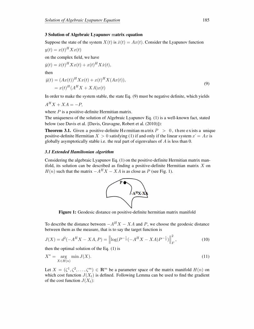
Considering the algebraic Lyapunov Eq. (1) on the positive-definite Hermitian matrix man-ifold, its solution can be described as finding a positive-definite Hermitian matrix X on H(n) such that the matrix −AHX − XA is as close as P (see Fig. 1).

Figure 1: Geodesic distance on positive-definite hermitian matrix manifold

To describe the distance between −AHX − XA and P , we choose the geodesic distancebetween them as the measure, that is to say the target function is

J(X) = d2(−AHX −XA,P ) =∥∥∥log(P− 1

2 (−AHX −XA)P−1

2 )∥∥∥2F, (10)

then the optimal solution of the Eq. (1) is

X∗ = argX∈H(n)

min J(X). (11)

Let X = (ζ1, ζ2, . . . , ζm) ∈ Rm be a parameter space of the matrix manifold H(n) onwhich cost function J(Xt) is defined. Following Lemma can be used to find the gradientof the cost function J(Xt):


Lemma 3.1 (Zhang [Zhang (2004)]). Let f(X) be the scalar function of the matrix X , ifdf(X) = tr(WdX) holds, then the gradient of f(X) with respect to X is

∂Xf(X) =WH . (12)

Theorem 3.2. Let J(X) be the function in (10), then the gradient of J(X) with respect tothe positive-definite Hermitian matrix X is

∂xJ(X) = P−1

2Y HP1

2 (AHX +XA)−1AH +AP−1

2Y HP1

2 (AHX +XA)−1

+ A(AHX +XA)−1P1

2Y HP−1

2 + (AHX +XA)−1P1

2Y P−1

2AH . (13)

Proof of the above Theorem see the Appendix.Theorem 3.3. On the positive definite Hermitian matrix system, if the i-th iteration matrixand direction matrix are Xi, Vi respectively, then (i + 1)-th iteration matrix and directionmatrix Xi+1, Vi+1 satisfy{Xi+1 = X

1

2

i exp(ηX− 1

2

i ViX− 1

2

i )X1

2

i ,

Vi+1 = η(ViX−1i Vi −∇Xi

J(Xi)) + (1− ηµ)Vi,(14)

where

∇XiJ(Xi) = Xi∂Xi

J(Xi)Xi,

the sufficient small number η is the learning rate, µ satisfies√2λm < µ < 1

η , λm isthe largest eigenvalue of the Hessian matrix of the cost function. The X and V iterationcontinue until the stopping criterion is met. See Fiori [Fiori (2011, 2012)] for more details.

By these discussion, we present the extended Hamiltonian algorithm to find the solution ofthe algebraic Lyapunov Eq. (1) on the positive-definite Hermitian matrix manifold H(n).Algorithm 3.1. For the manifold H(n) the algorithm is given as follows. Here J(X) isthe cost function (10).

1. Input initial matrix X0, initial direction V0, step size η and error tolerance ε > 0;

2. Calculate the gradient ∂XiJ(Xi) by (13);

3. If J(Xi) < ε, then halt;4. Update X , V according to (14) and go back to step 2.

3.1.1 Numerical experiment

Consider the submanifold PH(2) of H(2) defined by:

PH(2) =

{[ζ1 ζ2 + iζ3

ζ2 − iζ3 ζ4

]; ζi ∈ R, ζ1 > 0, ζ1ζ4 − (ζ2)2 − (ζ3)2 > 0

}. (15)

Now we consider the algebraic Lyapunov equation on the manifold of positive-definiteHermitian matrices.

AHX +XA+ P = 0,

where

A =

[−2 −1− ii −1

]


is any matrix with real part of its eigenvalues negative by Theorem 3.1,and

P =

[3 1 + 3

2 i1− 3

2 i 3

]∈ PH(2).

In this experiment, we choose initial guess X0 and initial direction V0 as

X0 =

[0.8 −0.3i0.3i 2.2

]∈ PH(2)

V0 =

[−0.5 −0.1 + 0.2i

−0.1− 0.2i −0.5

]∈ H ′(2)

Taking the step size η = 0.1 and µ = 6, then after 41 iterations, we obtain the optimalsolution under the error tolerance ε = 10−3 as follows,[

0.9968 0.0013− 0.4947i0.0013 + 0.4947i 1.9895

].

In fact, the exact solution of (1) on the positive-definite Hermitian matrix manifold in thisexample is[

1 −0.5i0.5i 2

].

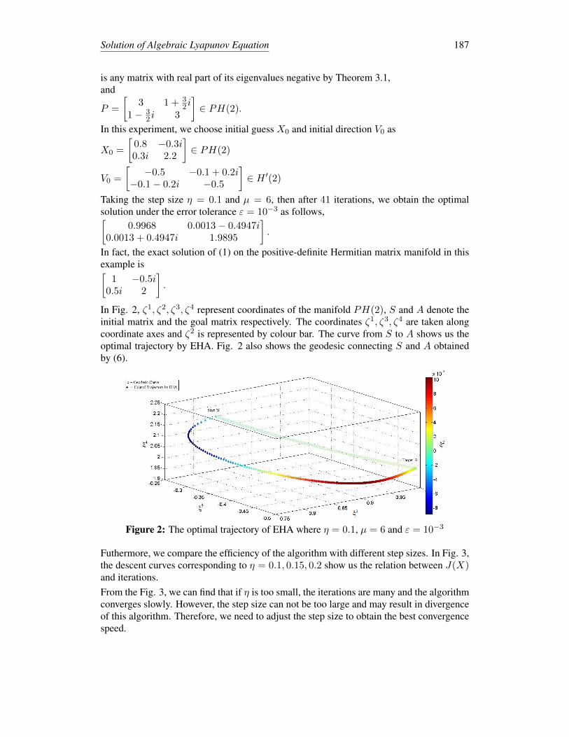
In Fig. 2, ζ1, ζ2, ζ3, ζ4 represent coordinates of the manifold PH(2), S and A denote theinitial matrix and the goal matrix respectively. The coordinates ζ1, ζ3, ζ4 are taken alongcoordinate axes and ζ2 is represented by colour bar. The curve from S to A shows us theoptimal trajectory by EHA. Fig. 2 also shows the geodesic connecting S and A obtainedby (6).

Figure 2: The optimal trajectory of EHA where η = 0.1, µ = 6 and ε = 10−3

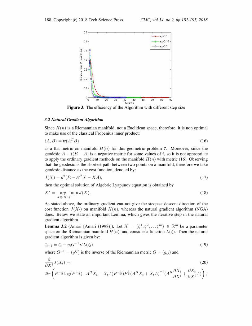
Futhermore, we compare the efficiency of the algorithm with different step sizes. In Fig. 3,the descent curves corresponding to η = 0.1, 0.15, 0.2 show us the relation between J(X)and iterations.From the Fig. 3, we can find that if η is too small, the iterations are many and the algorithmconverges slowly. However, the step size can not be too large and may result in divergenceof this algorithm. Therefore, we need to adjust the step size to obtain the best convergencespeed.


Figure 3: The efficiency of the Algorithm with different step size

3.2 Natural Gradient Algorithm

Since H(n) is a Riemannian manifold, not a Euclidean space, therefore, it is non optimalto make use of the classical Frobenius inner product:

〈A,B〉 = tr(ATB) (16)

as a flat metric on manifold H(n) for this geometric problem ?. Moreover, since thegeodesic A + t(B − A) is a negative metric for some values of t, so it is not appropriateto apply the ordinary gradient methods on the manifold H(n) with metric (16). Observingthat the geodesic is the shortest path between two points on a manifold, therefore we takegeodesic distance as the cost function, denoted by:

J(X) = d2(P,−AHX −XA), (17)

then the optimal solution of Algebric Lyapunov equation is obtained by

X∗ = argX∈H(n)

min J(X). (18)

As stated above, the ordinary gradient can not give the steepest descent direction of thecost function J(Xt) on manifold H(n), whereas the natural gradient algorithm (NGA)does. Below we state an important Lemma, which gives the iterative step in the naturalgradient algorithm.Lemma 3.2 (Amari [Amari (1998)]). Let X = (ζ1, ζ2, . . . ζm) ∈ Rm be a parameterspace on the Riemannian manifold H(n), and consider a function L(ζ). Then the naturalgradient algorithm is given by:

ζt+1 = ζt − ηtG−1∇L(ζt) (19)

where G−1 = (gij) is the inverse of the Riemannian metric G = (gij) and

∂

∂XiJ(Xt) = (20)

2tr

(P−

1

2 log(P−1

2 (−AHXt −XtA)P− 1

2 )P1

2 (AHXt +XtA)−1

(AH∂Xt

∂Xi+∂Xt

∂XiA)

),


Now, we will give the natural gradient descent algorithm for the considered Eq. (1), takingthe geodesic distance J(Xt) as the cost function and the negative of the gradient of the costfunction J(Xt) about Xt to give the descent direction in the iterative equation.Theorem 3.4. The iteration on manifold H(n) is given by

Xt+1 = Xt − ηG−1∇J(Xt), (21)

where the component of gradient ∇J(Xt) satisfies

∂J(Xt)

∂Xi= 2tr(P−

1

2 log(P−1

2 (−AHXt −XtA)P− 1

2

(AHXt +XtA)−1(AH

∂Xt

∂Xi+∂Xt

∂XiA), (22)

where i = 1, 2, . . . ,m.

For Proof of above Theorem See the Appendix.By these discussion, we present the natural gradient algorithm to find the solution of thealgebraic Lyapunov Eq. (1) on the manifold H(n) of positive-definite Hermitian matrices.Algorithm 3.2. For the coordinateX = (ζ1, ζ2, . . . , ζm) of the considered manifold H(n),the natural gradient algorithm is given by;

1. Set X◦ = (ζ1◦ , ζ2◦ , . . . , ζ

m◦ ) as the initial input matrix X and choose required toler-

ance ε◦ > 0.

2. Compute J(Xt) = d2(P,−AHXt −XtA)

3. If ‖∇J(Xt)‖F < ε◦, then halt.

4. Update the vector X by Xt+1 = Xt−ηG−1∇J(Xt), where Xt = (ζ1t , ζ2t , . . . , ζ

mt ),

η is learning rate and go back to step 2.

3.2.1 Numerical Simulations


PH(2) =

{[ζ1 ζ2 + iζ3

ζ2 − iζ3 ζ4

]; ζi ∈ R, ζ1 > 0, ζ1ζ4 − (ζ2)2 − (ζ3)2 > 0

}. (23)

Now we consider the algebraic Lyapunov equation on the manifold of positive-definiteHermitian matrices:

AHX +XA+ P = 0,

where

A =

[−2 −1− ii −1

]is any matrix with real part of its eigenvalues negative by Theorem 3.1,and

P =

[3 1 + 3

2 i1− 3

2 i 3

]∈ PH(2).


In this experiment, we choose initial guess X0 as

X0 =

[0.8 −0.3i0.3i 2.2

]∈ PH(2)

Taking the step size η = 0.035, then after 44 iterations, we obtain the optimal solutionunder the error tolerance ε = 10−2 as follows,[

1.0046 −0.0002− 0.5048i−0.0002 + 0.5048i 2.0146

].

In fact, the exact solution of (1) in this example is:[1 −0.5i

0.5i 2

].

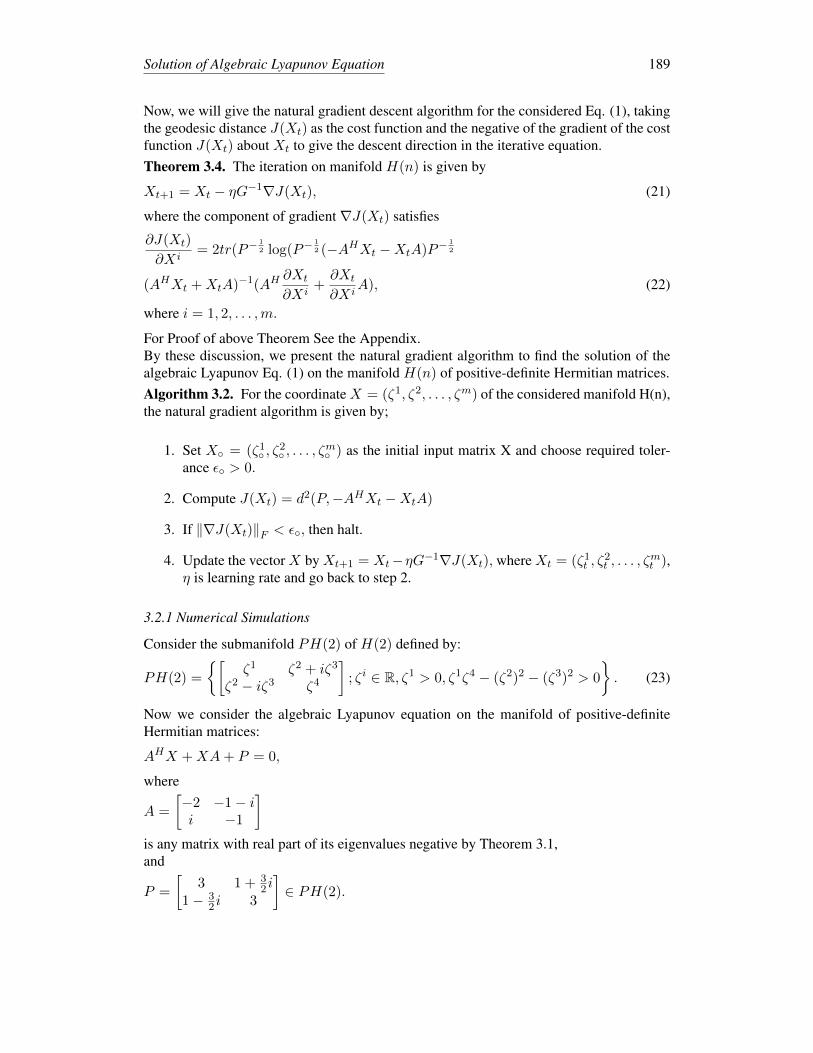
In Fig. 4, ζ1, ζ2, ζ3, ζ4 represent coordinates of the manifold PH(2), S and A denote theinitial matrix and the goal matrix respectively. The coordinates ζ1, ζ3, ζ4 are taken alongcoordinate axes and ζ2 is represented by colour bar. The curve from S to A shows us theoptimal trajectory by NGA. Fig. 4 also shows the geodesic connecting S and A obtainedby (6).

Figure 4: The optimal trajectory of NGA where η = 0.035 and ε = 10−2

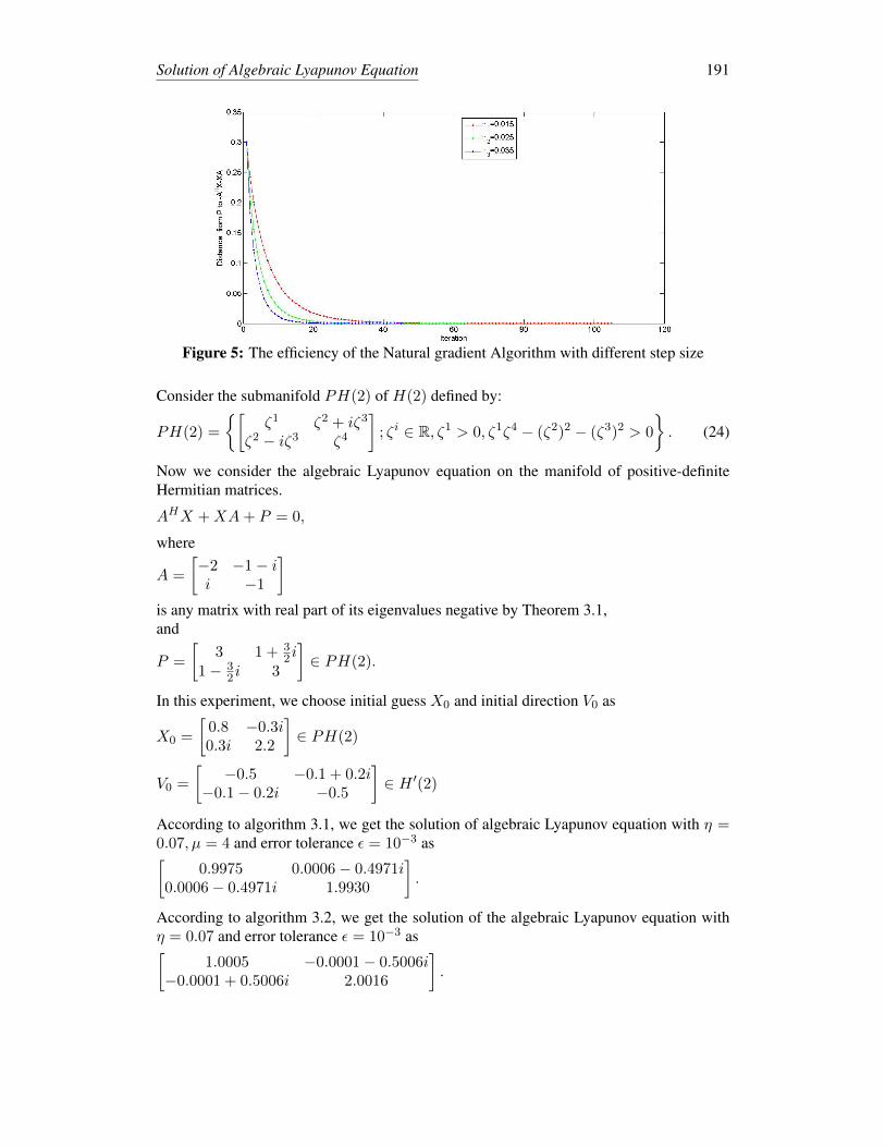
Futhermore, we compare the efficiency of the algorithm with different step sizes. In Fig. 5,the descent curves corresponding to η = 0.015, 0.025, 0.035 show us the relation betweenJ(X) and iterations.From the Fig. 5, we can find that if η is too smaller, the iterations are many and thealgorithm convergent slowly. However, the step size can not be too large, which may resultin divergence in this algorithm. Therefore, we need to adjust the step size in order to obtainthe best convergence speed.

3.3 Comparison of NGA and EHA

We apply the natural gradient algorithm 3.2 and extended Hamiltonian algorithm 3.1 tosolve the algebraic Lyapunov Eq. (1). From the following example, we can see the effi-ciency of the two proposed algorithms.


Figure 5: The efficiency of the Natural gradient Algorithm with different step size


PH(2) =

{[ζ1 ζ2 + iζ3

ζ2 − iζ3 ζ4

]; ζi ∈ R, ζ1 > 0, ζ1ζ4 − (ζ2)2 − (ζ3)2 > 0

}. (24)

Now we consider the algebraic Lyapunov equation on the manifold of positive-definiteHermitian matrices.

AHX +XA+ P = 0,

where

A =

[−2 −1− ii −1

]is any matrix with real part of its eigenvalues negative by Theorem 3.1,and

P =

[3 1 + 3

2 i1− 3

2 i 3

]∈ PH(2).

In this experiment, we choose initial guess X0 and initial direction V0 as

X0 =

[0.8 −0.3i0.3i 2.2

]∈ PH(2)

V0 =

[−0.5 −0.1 + 0.2i

−0.1− 0.2i −0.5

]∈ H ′(2)

According to algorithm 3.1, we get the solution of algebraic Lyapunov equation with η =0.07, µ = 4 and error tolerance ε = 10−3 as[

0.9975 0.0006− 0.4971i0.0006− 0.4971i 1.9930

].

According to algorithm 3.2, we get the solution of the algebraic Lyapunov equation withη = 0.07 and error tolerance ε = 10−3 as[

1.0005 −0.0001− 0.5006i−0.0001 + 0.5006i 2.0016

].


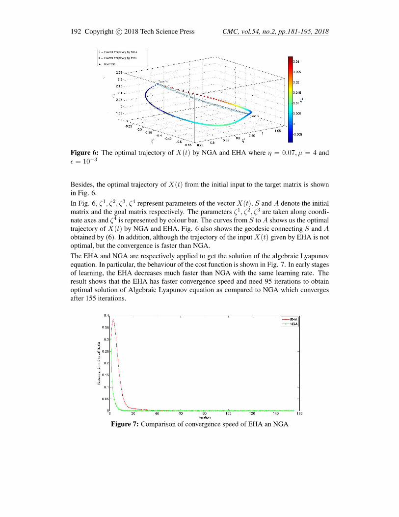
Figure 6: The optimal trajectory of X(t) by NGA and EHA where η = 0.07, µ = 4 andε = 10−3

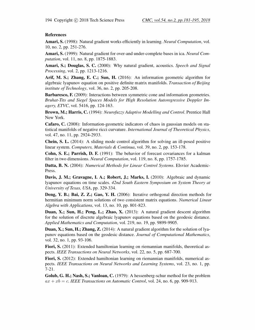
Besides, the optimal trajectory of X(t) from the initial input to the target matrix is shownin Fig. 6.In Fig. 6, ζ1, ζ2, ζ3, ζ4 represent parameters of the vector X(t), S and A denote the initialmatrix and the goal matrix respectively. The parameters ζ1, ζ2, ζ3 are taken along coordi-nate axes and ζ4 is represented by colour bar. The curves from S toA shows us the optimaltrajectory of X(t) by NGA and EHA. Fig. 6 also shows the geodesic connecting S and Aobtained by (6). In addition, although the trajectory of the input X(t) given by EHA is notoptimal, but the convergence is faster than NGA.The EHA and NGA are respectively applied to get the solution of the algebraic Lyapunovequation. In particular, the behaviour of the cost function is shown in Fig. 7. In early stagesof learning, the EHA decreases much faster than NGA with the same learning rate. Theresult shows that the EHA has faster convergence speed and need 95 iterations to obtainoptimal solution of Algebraic Lyapunov equation as compared to NGA which convergesafter 155 iterations.

Figure 7: Comparison of convergence speed of EHA an NGA


4 ConclusionWe studied the solution of continuous algebraic Lyapunov equation by considering thepositive-definite Hermitian matrices as a Riemannian manifold and used geodesic distanceto find the solution. Here we used two algorithms, the extended Hamiltonian algorithm andthe natural gradient algorithm to get the approximate solution of algebraic Lyapunov matrixequation. Finally, several numerical experiments give you an idea about the effectivenessof the proposed algorithms. We also show the comparison between these two algorithm-s EHA and NGA. Henceforth we conclude that the extended Hamiltonian algorithm hasbetter convergence speed than the natural gradient algorithm, whereas the trajectory of thesolution matrix is optimal in case of NGA as compared to EHA.

5 AppendixProof of Theorem 3.2Proof. Since −AHX −XA is Hermitian. Let Y = log(P−

1


2 )

dY = dlog(P−1


2 )

= (P−1


2 )−1P−1

2 (−AHdX − dXA)P−1

2 )

= P1

2 (−AHX −XA)−1(−AHdX − dXA)P−1

2

then, we have

dJ(X) = d(tr(Y HY )) = tr(dY HY + Y HdY )

According to Lemma 4.3.1, the geodesic of J(X) with respect to X is

∂xJ(X) = P−1

2Y HP1

2 (AHX +XA)−1AH +AP−1

2Y HP1

2 (AHX +XA)−1

+A(AHX +XA)−1P1

2Y HP−1

2 + (AHX +XA)−1P1

2Y P−1

2AH .

Proof of Theorem 3.4Proof. According to above Lemma, we can get the iterative process

Xt+1 = Xt − ηG−1∇J(Xt),

where the Fisher metric matrix G is obtained by 3. Let X(t) = log((−AHXt −XtA)− 1

2

P (−AHXt − XtA)− 1

2 ), it is easy to show that X(t) is Hermitian from (20) in Lemma3.2 and the properties of the trace of a matrix, we have the components of the gradient∇J(Xt):

∂

∂XiJ(Xt)=2tr

(log(P−

1

2 (−AHXt−XtA)P− 1

2 )∂

∂Xi(log(P−

1


2 ))

)=2tr

(P−

1

2 log(P−1


2 )P1

2 (−AHXt−XtA)−1(AH

∂Xt

∂Xi+∂Xt

∂XiA)

),

where i = 1, 2, . . . ,m.

Acknowledgement: The authors wish to express their appreciation to the reviewers fortheir helpful suggestions which greatly improved the presentation of this paper.


ReferencesAmari, S. (1998): Natural gradient works efficiently in learning. Neural Computation, vol. 10, no. 2, pp. 251-276.Amari, S. (1999): Natural gradient for over-and under-complete bases in ica. Neural Com-putation, vol. 11, no. 8, pp. 1875-1883.Amari, S.; Douglas, S. C. (2000): Why natural gradient, acoustics. Speech and Signal Processing, vol. 2, pp. 1213-1216.Arif, M. S.; Zhang, E. C.; Sun, H. (2016): An information geometric algorithm for algebraic lyapunov equation on positive definite matrix manifolds. Transaction of Beijing institute of Technology, vol. 36, no. 2, pp. 205-208.Barbaresco, F. (2009): Interactions between symmetric cone and information geometries. Bruhat-Tits and Siegel Spaces Models for High Resolution Autoregressive Doppler Im-agery, ETVC, vol. 5416, pp. 124-163.Brown, M.; Harris, C. (1994): Neurofuzzy Adaptive Modelling and Control. Prentice Hall New York.Cafaro, C. (2008): Information-geometric indicators of chaos in gaussian models on sta-tistical manifolds of negative ricci curvature. International Journal of Theoretical Physics, vol. 47, no. 11, pp. 2924-2933.Chein, S. L. (2014): A sliding mode control algorithm for solving an ill-posed positive linear system. Computers, Materials & Continua, vol. 39, no. 2, pp. 153-178.Cohn, S. E.; Parrish, D. F. (1991): The behavior of forecast covariances for a kalman filter in two dimensions. Neural Computation, vol. 119, no. 8, pp. 1757-1785.Datta, B. N. (2004): Numerical Methods for Linear Control Systems. Elsvier Academic-Press.Davis, J. M.; Gravagne, I. A.; Robert, J.; Marks, I. (2010): Algebraic and dynamic lyapunov equations on time scales. 42nd South Eastern Symposium on System Theory at University of Texas, USA, pp. 329-334.Deng, Y. B.; Bai, Z. Z.; Gao, Y. H. (2006): Iterative orthogonal direction methods for hermitian minimum norm solutions of two consistent matrix equations. Numerical Linear Algebra with Applications, vol. 13, no. 10, pp. 801-823.Duan, X.; Sun, H.; Peng, L.; Zhao, X. (2013): A natural gradient descent algorithm for the solution of discrete algebraic lyapunov equations based on the geodesic distance. Applied Mathematics and Computation, vol. 219, no. 19, pp. 9899-9905.Duan, X.; Sun, H.; Zhang, Z. (2014): A natural gradient algorithm for the solution of lya-punov equations based on the geodesic distance. Journal of Computational Mathematics, vol. 32, no. 1, pp. 93-106.Fiori, S. (2011): Extended hamiltonian learning on riemannian manifolds, theoretical as-pects. IEEE Transactions on Neural Networks, vol. 22, no. 5, pp. 687-700.Fiori, S. (2012): Extended hamiltonian learning on riemannian manifolds, numerical as-pects. IEEE Transactions on Neural Networks and Learning Systems, vol. 23, no. 1, pp. 7-21.Golub, G. H.; Nash, S.; Vanloan, C. (1979): A hessenberg-schur method for the problem ax + xb = c. IEEE Transactions on Automatic Control, vol. 24, no. 6, pp. 909-913.


Jbilou, K. (2010): Adi preconditioned krylov methods for large lyapunov matrix equations. Linear Algebra & Its Applications, vol. 432, no. 10, pp. 2473-2485.Li, J. R.; White, J. (2002): Low-rank solution of lyapunov equations. SIAM Journal on Matrix Analysis and Applications, vol. 24, no. 1, pp. 260-280.Luo, Z.; Sun, H. (2014): Extended hamiltonian algorithm for the solution of discrete algebraic lyapunov equations. Applied Mathematics and Computation, vol. 234, pp. 245-252.Moakher, M. (2005): A differential geometric approach to the geometric mean of sym-metric positive-definite matrices. SIAM Journal on Matrix Analysis and Applications, vol. 26, no. 3, pp. 735-747.Moakher, M.; Batcherlor, P. G. (2006): Symmetric Positive-Definite M atrices: From Geometry to Applications and Visualizatin, Visualization and Processing of Tensor Fields. Springer.Ran, A. C. M.; Reurings, M. C. B. (2004): A fixed point theorem in partially ordered sets and some applications to matrix equations. Proceedings of the American Mathematical Society, vol. 132, pp. 1435-1443.Su, Y. F.; Chen, G. L. (2010): Iterative methods for solving linear matrix equation and linear matrix system. Numerical Linear Algebra with Applications, vol. 87, no. 4, pp. 763-774.Vandereycken, B.; Vandewalle, S. (2010): A riemannian optimization approach for com-puting low-rank solutions of lyapunov equations. SIAM Journal on Matrix Analysis and Applications, vol. 31, no. 5, pp. 2553-2579.Zhang, X. D. (2004): Matrix Analysis and Application. Springer, Beijing.

Solution of Algebraic Lyapunov Equation on Positive … [email protected] 2Department...

Documents

Transcript of Solution of Algebraic Lyapunov Equation on Positive … [email protected] 2Department...