Predictingchaosfor infinite dimensionaldynamicalsystems ...Kuramoto-Sivashinskyequation, acase study...
4
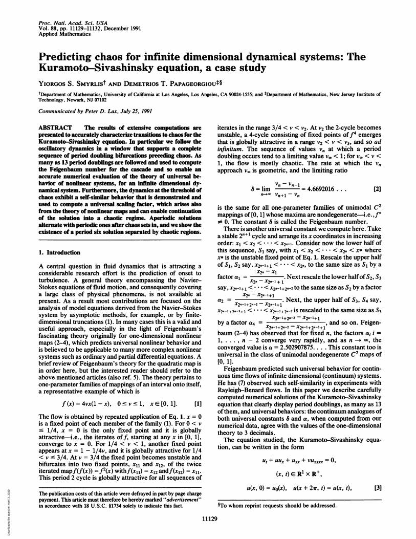
Proc. Nati. Acad. Sci. USA Vol. 88, pp. 11129-11132, December 1991 Applied Mathematics Predicting chaos for infinite dimensional dynamical systems: The Kuramoto-Sivashinsky equation, a case study YIORGOS S. SMYRLISt AND DEMETRIOS T. PAPAGEORGIOU0§ tDepartment of Mathematics, University of California at Los Angeles, Los Angeles, CA 90024-1555; and tDepartment of Mathematics, New Jersey Institute of Technology, Newark, NJ 07102 Communicated by Peter D. Lax, July 25, 1991 ABSTRACT The results of extensive computations are presented to accurately characterize transitions to chaos for the Kuramoto-Sivashinsky equation. In particular we follow the oscillatory dynamics in a window that supports a complete sequence of period doubling bifurcations preceding chaos. As many as 13 period doublings are followed and used to compute the Feigenbaum number for the cascade and so enable an accurate numerical evaluation of the theory of universal be- havior of nonlinear systems, for an infinite dimensional dy- namical system. Furthermore, the dynamics at the threshold of chaos exhibit a self-similar behavior that is demonstrated and used to compute a universal scaling factor, which arises also from the theory of nonlinear maps and can enable continuation of the solution into a chaotic regime. Aperiodic solutions alternate with periodic ones after chaos sets in, and we show the existence of a period six solution separated by chaotic regions. 1. Introduction A central question in fluid dynamics that is attracting a considerable research effort is the prediction of onset to turbulence. A general theory encompassing the Navier- Stokes equations of fluid motion, and consequently covering a large class of physical phenomena, is not available at present. As a result most contributions are focused on the analysis of model equations derived from the Navier-Stokes system by asymptotic methods, for example, or by finite- dimensional truncations (1). In many cases this is a valid and useful approach, especially in the light of Feigenbaum's fascinating theory originally for one-dimensional nonlinear maps (2-4), which predicts universal nonlinear behavior and is believed to be applicable to many more complex nonlinear systems such as ordinary and partial differential equations. A brief review of Feigenbaum's theory for the quadratic map is in order here, but the interested reader should refer to the above mentioned articles (also ref. 5). The theory pertains to one-parameter families of mappings of an interval onto itself, a representative example of which is f (x) =4vx( - x), 0 < v-l, x E [, 1]. Ill The flow is obtained by repeated application of Eq. 1. x = 0 is a fixed point of each member of the family (1). For 0 < v < 1/4, x = 0 is the only fixed point and it is globally attractive-i.e., the iterates of f, starting at any x in [0, 1], converge to x = 0. For 1/4 < v < 1, another fixed point appears at x = 1 - 1/4v, and it is globally attractive for 1/4 < v - 3/4. At v = 3/4 the fixed point becomes unstable and bifurcates into two fixed points, x1l and x12, of the twice iterated mapf(f(x)) =J2(x) withf(x1j) = x12 andf(x12) = x11. This period 2 cycle is globally attractive for all sequences of iterates in the range 3/4 < v < v2. At v2 the 2-cycle becomes unstable, a 4-cycle consisting of fixed points of f4 emerges that is globally attractive in a range v2 < v < V3, and so ad infinitum. The sequence of values v,, at which a period doubling occurs tend to a limiting value v. < 1; for v. < v < 1, the flow is mostly chaotic. The rate at which the vn approach v. is geometric, and the limiting ratio vn -vn-l 8 = lim = 4.6692016 . . . n-"o vn+-Vn [2] is the same for all one-parameter families of unimodal C2 mappings of [0, 1] whose maxima are nondegenerate-i.e.,f" $ 0. The constant 8 is called the Feigenbaum number. There is another universal constant we compute here. Take a stable 2"+1 cycle and arrange its x coordinates in increasing order: x1 < x2 < * * * < X2,+i. Consider now the lower half of this sequence, Si say, with x1 < x2 < ... < X2, < x* where x* is the unstable fixed point of Eq. 1. Rescale the upper half of S1, S2 say, X2.-1+1 < ... < x2, to the same size as S1 by a X2n -X1 factor a, = . Next rescale the lower half of S2, 53 X2" - X2.-1 + 1 say, X2.-Il1 < ... <X2n-1+2-2 to the same size as S2 by a factor X2" - X2n-1+l a2 = . Next, the upper half of S3, S4 say, X2n-l+2n-2 X2n-l+l X2.-l+2x-3+1 < ... * < X2-1+2-2 is rescaled to the same size as S3 X2.1-1+2n-2 - X2.-1+1 by a factor a4 = and so on. Feigen- X2,-1 +2-2 X2n-1+2R-3+1 baum (2-4) has observed that for fixed n, the factors ai i = 1, . .. , n - 2 converge very rapidly, and as n -a 00, the converged value is a = 2.502907875.... This constant too is universal in the class of unimodal nondegenerate C2 maps of [0, 1]. Feigenbaum predicted such universal behavior for contin- uous time flows of infinite dimensional (continuum) systems. He has (7) observed such self-similarity in experiments with Rayleigh-Benard flows. In this paper we describe carefully computed numerical solutions of the Kuramoto-Sivashinsky equation that clearly display period doublings, as many as 13 of them, and universal behaviors: the continuum analogues of both universal constants 8 and a, when computed from our numerical data, agree with the values of the one-dimensional theory to 3 decimals. The equation studied, the Kuramoto-Sivashinsky equa- tion, can be written in the form ut + uUX + urX + vUxXXX = 0, (x, t) ER1 X R+, u(x, 0) = uo(x), u(x + 21r, t) = u(x, t), §To whom reprint requests should be addressed. 11129 The publication costs of this article were defrayed in part by page charge payment. This article must therefore be hereby marked "advertisement" in accordance with 18 U.S.C. §1734 solely to indicate this fact. [31 Downloaded by guest on April 3, 2020
Transcript of Predictingchaosfor infinite dimensionaldynamicalsystems ...Kuramoto-Sivashinskyequation, acase study...
Proc. Nati. Acad. Sci. USAVol. 88, pp. 11129-11132, December 1991Applied Mathematics
Predicting chaos for infinite dimensional dynamical systems: TheKuramoto-Sivashinsky equation, a case studyYIORGOS S. SMYRLISt AND DEMETRIOS T. PAPAGEORGIOU0§tDepartment of Mathematics, University of California at Los Angeles, Los Angeles, CA 90024-1555; and tDepartment of Mathematics, New Jersey Institute ofTechnology, Newark, NJ 07102
Communicated by Peter D. Lax, July 25, 1991
ABSTRACT The results of extensive computations arepresented to accurately characterize transitions to chaos for theKuramoto-Sivashinsky equation. In particular we follow theoscillatory dynamics in a window that supports a completesequence of period doubling bifurcations preceding chaos. Asmany as 13 period doublings are followed and used to computethe Feigenbaum number for the cascade and so enable anaccurate numerical evaluation of the theory of universal be-havior of nonlinear systems, for an infinite dimensional dy-namical system. Furthermore, the dynamics at the threshold ofchaos exhibit a self-similar behavior that is demonstrated andused to compute a universal scaling factor, which arises alsofrom the theory of nonlinear maps and can enable continuationof the solution into a chaotic regime. Aperiodic solutionsalternate with periodic ones after chaos sets in, and we show theexistence of a period six solution separated by chaotic regions.
1. Introduction
A central question in fluid dynamics that is attracting aconsiderable research effort is the prediction of onset toturbulence. A general theory encompassing the Navier-Stokes equations of fluid motion, and consequently coveringa large class of physical phenomena, is not available atpresent. As a result most contributions are focused on theanalysis of model equations derived from the Navier-Stokessystem by asymptotic methods, for example, or by finite-dimensional truncations (1). In many cases this is a valid anduseful approach, especially in the light of Feigenbaum'sfascinating theory originally for one-dimensional nonlinearmaps (2-4), which predicts universal nonlinear behavior andis believed to be applicable to many more complex nonlinearsystems such as ordinary and partial differential equations. Abrief review of Feigenbaum's theory for the quadratic map isin order here, but the interested reader should refer to theabove mentioned articles (also ref. 5). The theory pertains toone-parameter families of mappings ofan interval onto itself,a representative example of which is
f (x) =4vx( - x), 0 <v-l, xE[, 1]. Ill
The flow is obtained by repeated application of Eq. 1. x = 0is a fixed point of each member of the family (1). For 0 < v< 1/4, x = 0 is the only fixed point and it is globallyattractive-i.e., the iterates of f, starting at any x in [0, 1],converge to x = 0. For 1/4 < v < 1, another fixed pointappears at x = 1 - 1/4v, and it is globally attractive for 1/4< v - 3/4. At v = 3/4 the fixed point becomes unstable andbifurcates into two fixed points, x1l and x12, of the twiceiterated mapf(f(x)) =J2(x) withf(x1j) = x12 andf(x12) = x11.This period 2 cycle is globally attractive for all sequences of
iterates in the range 3/4 < v < v2. At v2 the 2-cycle becomesunstable, a 4-cycle consisting of fixed points off4 emergesthat is globally attractive in a range v2 < v < V3, and so adinfinitum. The sequence of values v,, at which a perioddoubling occurs tend to a limiting value v. < 1; for v. < v <1, the flow is mostly chaotic. The rate at which the vnapproach v. is geometric, and the limiting ratio
vn -vn-l8 = lim = 4.6692016 . . .
n-"o vn+-Vn[2]
is the same for all one-parameter families of unimodal C2mappings of [0, 1] whose maxima are nondegenerate-i.e.,f"$ 0. The constant 8 is called the Feigenbaum number.There is another universal constant we compute here. Take
a stable 2"+1 cycle and arrange its x coordinates in increasingorder: x1 <x2 < * * * < X2,+i. Consider now the lower half ofthis sequence, Si say, with x1 <x2 < ... < X2, < x* wherex* is the unstable fixed point of Eq. 1. Rescale the upper halfof S1, S2 say, X2.-1+1 < ... <x2, to the same size as S1 by a
X2n -X1factor a, = . Next rescale the lower halfofS2, 53
X2" - X2.-1 + 1
say, X2.-Il1 <... <X2n-1+2-2 to the same size as S2 by a factorX2"- X2n-1+l
a2 = . Next, the upper half of S3, S4 say,X2n-l+2n-2 X2n-l+l
X2.-l+2x-3+1 <... * <X2-1+2-2 is rescaled to the same size as S3X2.1-1+2n-2 - X2.-1+1
by a factor a4 = and so on. Feigen-X2,-1+2-2 X2n-1+2R-3+1
baum (2-4) has observed that for fixed n, the factors ai i =1, . .. , n - 2 converge very rapidly, and as n -a 00, theconverged value is a = 2.502907875.... This constant too isuniversal in the class of unimodal nondegenerate C2 maps of[0, 1].Feigenbaum predicted such universal behavior for contin-
uous time flows of infinite dimensional (continuum) systems.He has (7) observed such self-similarity in experiments withRayleigh-Benard flows. In this paper we describe carefullycomputed numerical solutions of the Kuramoto-Sivashinskyequation that clearly display period doublings, as many as 13ofthem, and universal behaviors: the continuum analogues ofboth universal constants 8 and a, when computed from ournumerical data, agree with the values of the one-dimensionaltheory to 3 decimals.The equation studied, the Kuramoto-Sivashinsky equa-
tion, can be written in the form
ut + uUX + urX + vUxXXX = 0,
(x, t)ER1 X R+,
u(x, 0) = uo(x), u(x + 21r, t) = u(x, t),
§To whom reprint requests should be addressed.
11129
The publication costs of this article were defrayed in part by page chargepayment. This article must therefore be hereby marked "advertisement"in accordance with 18 U.S.C. §1734 solely to indicate this fact.
[31
Dow
nloa
ded
by g
uest
on
Apr
il 3,
202
0
11130 Applied Mathematics: Smyrlis and Papageorgiou
Table 1. Overview of the most attracting manifoldsDescription of the
Window range attractors1 < v < 00 Trivial solution
0.25 < v < 1 Steady state of period 2wr0.0756 < v < 0.025 Steady state of period ir
0.06697 5 v < 0.0755 Steady state of period 2ir0.05992 < v s 0.06695 Steady state of period 2ir/30.05516 s v < 0.05991 Time periodic attractor
0.0396227 s v < 0.05515 Steady state of period 2ir0.03729 5 v < 0.0396226 Time periodic attractor
0.0346259 < v < 0.03728 Steady state of period ir/20.029969103484 < v < 0.0346258 Time periodic attractor
containing completeperiod-doubling sequence
0.02922 _ v < 0.02969910348 Chaotic oscillations0.02905 < v _ 0.02921 Time periodic attractor0.02855 _ v _ 0.02904 Chaotic oscillations0.02662 _ v _ 0.02854 Time periodic attractor0.02525 < v _ 0.02661 Chaotic oscillations0.02506 _ v < 0.02524 Time periodic attractor
0.0248607 _ v _ 0.02505 Chaotic oscillations0.02445 _ v _ 0.0248606 Time periodic attractor
containing completeperiod-doubling sequence
0.0242861 < v s 0.02445 Chaotic oscillations0.02367 < v c 0.02438608 Time periodic attractor
containing completeperiod-doubling sequence
0.0232 c v 5 0.02386 Chaotic oscillations0.0229 < v < 0.0231 Time periodic attractor0.0223 5 v < 0.0228 Chaotic oscillations0.022 < v < 0.0222 Time periodic attractor
? v < 0.0219 Chaotic oscillations
Table 2. Computation of the Feigenbaum numberSubwindow Ratio of
Subwindow boundary v length lengths Time period0.0346258 4.3083 x 10⁻³ - 0.440.03031749 2.6825 x 10⁻⁴ 0.880.030049233 6.2786 x 10⁻⁵ 16.061 1.760.029986446 1.3609 x 10⁻⁵ 4.2724 3.520.0299728366 2.9330 x 10⁻⁶ 4.6136 7.030.0299699036 6.288 x 10⁻⁷ 4.6399 14.050.02996927484 1.3456 x 10⁻⁷ 4.6644 28.10.02996914018 2.884 x 10⁻⁸ 4.6657 56.20.02996911134 6.18 x 10⁻⁹ 4.667 112.40.02996910516 1.32 x 10⁻⁹ 4.68 224.80.029969103842 2.84 x 10⁻¹⁰ 4.65 449.60.029969103558 6.0 x 10⁻¹¹ 4.7 899.10.029969103498 1.4 x 10⁻¹¹ 4. 1798.20.029969103484 00
2. Numerical solutions.
The results presented here were obtained by numericalsolution of the initial value problem (Eq. 3) with the initialcondition
uo(x) = -sin(x),
for all values of v. Since solutions of Eq. 3 are uniquelydetermined by their initial data, a solution that is an oddfunction ofx initially will remain so for all subsequent times.The advantage of such a choice is that there exist analyticalresults that give global bounds for u(x, t) and higher deriva-tives in the odd-parity case (14); the bounds available in thegeneral case grow exponentially in t (15). The numericalscheme is a Galerkin spectral method based on a sine series
where v > 0 is the viscosity of the system. This equationarises in a variety of problems such as concentration waves
(8), flame propagation (9), free surface flows (10). A gener-alized form, ofwhich Eq. 3 is a special case, has been derivedby an asymptotic analysis of the Navier-Stokes equations inthe context oftwo-phase flows in cylindrical geometries withapplications in lubricated pipe-lining (for the efficient trans-port of crude oil) and oil recovery through porous media (11).Much analytical and computational work has been completedto describe the complicated nonlinear dynamics that Eq. 3can produce as v varies and, in particular, when it achievesfairly small values (see refs. 12 and 13).
Spai c-tinic profile of perilic alttractor8100
~~ ~ ~ ~ ~ ~ rir - -.-)181t
FIG. 1. Spatio-temporal evolution at v =0.03. Solution has
undergone two period doublings and is en route to chaos.
v = 0.030550c40.3020100
-10
-20-
-30
-40
-50L14 15 16 17 18 19 20 21 Z
Period = 0.445588785
v = 0.030150-403020100
-10-20-30-40-CAI
4 15 16 17 18 19 20 21 22
Period = 0.8841534755
v = 0.035040
30
20
10.0
-10
-20-
-30
-40
"v14 15 16 17 18 19 20 21 22Period = 1.758719370
v = 0.02998
4 15 16 17 14 19 0 21Period = 3.51437820
4 15 16 17 18 19 20 21 .Period = 7.02511715935
v = 0.0299695
-50
40.
30
20
-20-10
-30
-40
5014 15 16 17 18 19 20 21 22
Period 14.04917616
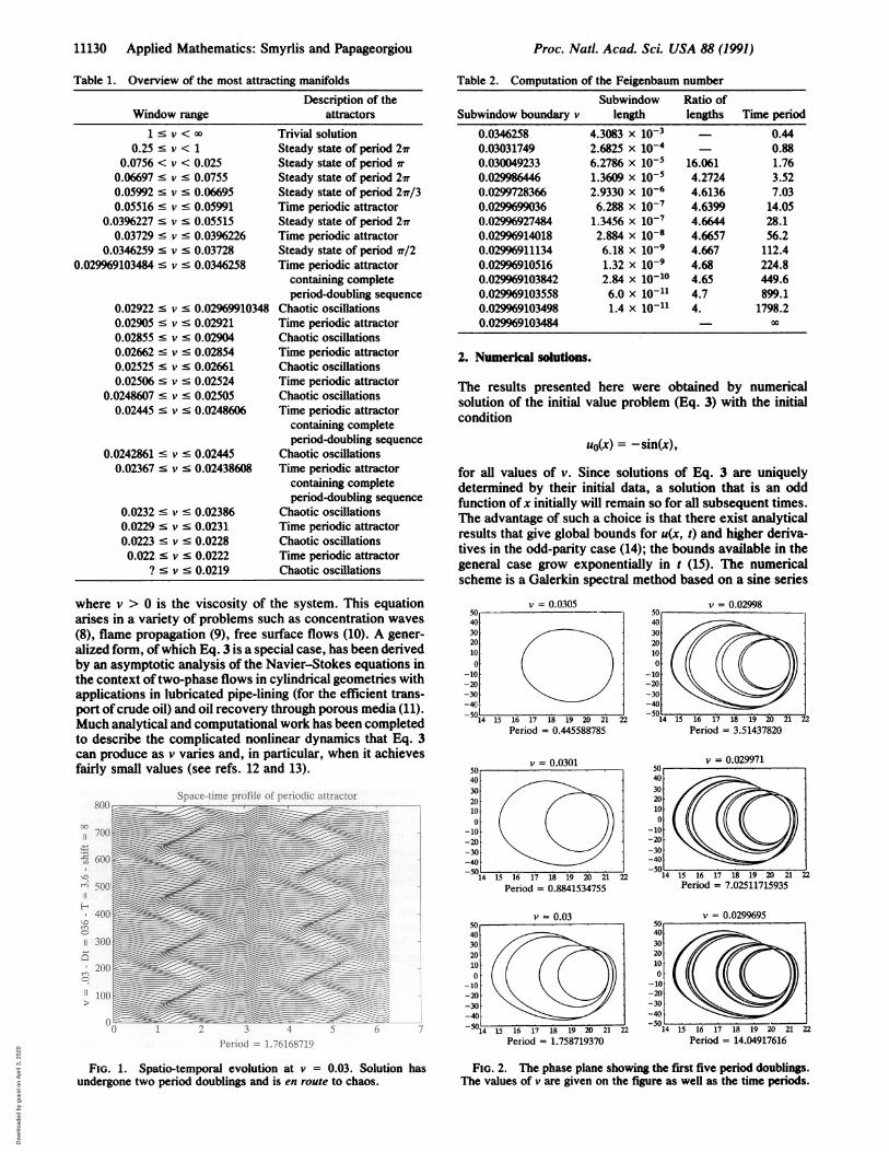
FIG. 2. The phase plane showing the first five period doublings.The values of v are given on the figure as well as the time periods.
403020100
-10-20-30-40-50
Proc. Natl. Acad Sci. USA 88 (1991)
2
2
Dow
nloa
ded
by g
uest
on
Apr
il 3,
202
0
Applied Mathematics: Smyrlis and Papageorgiou
a Minima of energy phase plane0.01-
0.005-I
-0.0051-0.011 16 18
1/16 of minima 1/32 of miniman ni
0.005-r
0
17.3 17.35
g 001 1/64 of minima
0005
0
-0005 j
17.345 17.35 17.355
00.01 1/256 of minima
0.005
0
-0.005
0117.351 17.352 17.353v 0.0299691035
I -
-117.34 17.36 17.3E
1/128 of minima0.01 *: .*.
0.005
0
-0.005
-00117.352 17.354 17.356
1/512 of minima0U1
0.005
0
-0.005
-00117.352 17.353 17.35
Period= 1798.2564595
FIG. 3. Successive magnification of the energy minima of212-cycle, showing the self-similar characteristics of the attracto
and is described in detail in ref. 12. The truncation orderthe Galerkin approximation depends on the value of vcrude estimate that has proven practical shows that it suffikto retain a few frequencies more than v-12, the numberlinearly unstable ones around u = 0. Taking any mefrequencies does not change the computed solution; tnumber is an upper bound on the dimension of the attractIn ref. 16 it was shown that'the Hausdorff dimension ofattractor does not exceed- const v-2/"0, which is larger ttv112 by a factor of const v-1/40; the constant, however,very large.
Since the Kuramoto-Sivashinsky equation (Eq. 3) isconservative form, f? u(x, t)dx is a conserved quantityhas been proved that when v > 1, every solution whiintegral is zero initially tends to zero uniformly; this is bolout by our numerical calculations. As we decrease v belo%the zero solution becomes unstable, bifurcates, and tendslarge t to a steady nonconstant state. When v decreases belt1/4, u tends to a new linearly stable steady state whose spalperiod is ir. Further decrease of v gives stable steady staof spatial period 2rand 21r/3. At v = 0.05991, atime-perioattractor is found; a single period doubling occurs in t
f FIG. 4. Route to chaos and beyond for the minima of the energyof the Kuramoto-Sivashinsky equation. Disorder sets in as theviscosity v decreases from right to left. The v axis has been enlargedby a factor of 100.
window (by window we mean intervals of v that attractqualitatively similar solutions), but as v is decreased further,the solutions are' attracted to steady states of spatial period2ir. Next we find a new time-periodic window with two
h period doublings and one period halving. Further decrease ofv gives steady states with spatial period wr/2. Next we find athird periodic window that contains a complete sequence ofperiod-doubling bifurcations (we could identify 13), whichlead to chaos, and so on (see Table 1).A graphical view of the solutions at v = 0.03 is presented
in Fig. 1. The time period here-is 1.76168719, and we are inthe subwindow directly after the second period-doubling.The spatial and temporal evolution of the profile are collec-tively shown over a domain x E [0, 2Xr] with u on the verticalaxis and x on the horizontal axis. One hundred profiles areplotted at time intervals of 0.036 and shifted vertically by adistance of 8 units. The whole duration of the picture is 3.6time units and contains approximately two time periods.Computation of the Feigenbaum Number. Table 2 presents
our evidence that verifies Feigenbaum's universal theory forthe Kuramoto-Sivashinsky equation. These results weregenerated by monitoring the evolution of the energy, E(t)-
the i.e., the L2-norm of the solution. Each entry in Table 2ir. represents the beginning of successive subwindows, which
support solutions that undergo period doublings. The sharpestimation of these borundaries-is necessary if an accurate
of computation of the Feigenbaum number is desired. In alli;acesoforehis:or.theian, is
, in. ItDsemeii,
forowtialltesdichis
1
-.
1-
I .
II
14.3
FIG. 5. Enlargement of Fig. 4 route to chaos for the minima oftheenergy of the Kuramoto-Sivashinsky equation. The 6-cycle solutionis seen between 2.992 and 2.993.
1/2 of minimaI0.01 +/ - --. b:0.005-
0
-0.005-D17 18
14,9E~'___)m);a.1)1.... '. ) ()! ()f
U.')'
0.005
-0.005
Ii
Proc. Nad. Acad. Sci. USA 88 (1991) 11131
e n nil
Dow
nloa
ded
by g
uest
on
Apr
il 3,
202
0

11132 Applied Mathematics: Smyrlis and Papageorgiou
results reported here, the, boundaries were estimated withenough accuracy to yield the Feigenbaum number correct tothe number of significant figures shown. The first columngives the value of v where the subwindow begins, the secondcolumn gives' the subwindow length, the third column givesthe ratio of successive subwindow lengths according to Eq.2, and the fourth column gives the time period of theoscillation. Fig. 2 shows representative energy phase planes,generated by plotting E(t) versus E(t), for the first five perioddoublings. The overall limits of these phase planes (forexample, the maximum -and minimum ofE and E) do not varymuch beyond the second period doubling. Period doubling isindicated by the appearance of more turns in the phase plane(i.e., by an index change of the curves-the way in which thephase plane gains more turns before the appearance of chaosis quantified in the next subsection.The Universal Limit of Multiple Period Doubflngs. Next we
present a set of numerical results that exhibit very clearly theself-similar nature of period-doubling bifurcations. The ex-periment we choose has a value of v ='0.0299691035 and liesat the end of the third periodic window; at a value sof v =0.029969103484-i.e., a decrease of 1.6 x 10¹¹-chaoticsolutions are' observed. The time period of the solution is1798.2564595 units and is the result of a sequence of 12 perioddoublings (in Fig. 1 we show only the first 5). The energy E(t)of this solution is a scalar-valued periodic function; becauseof the 12 period doublings, it has 211 local minima in oneperiod. We arrange these in increasing order E1 < E2 < *< E21i. In Fig. 3a, we picture these values by drawing avertical line through each E,, i = 1, .. , 21. In Fig. 3b-wepicture the upper half of these energy minima El,i = 210 + 1,.. ., 21, rescaled to the same size by the factor a,
E21 -ElE=~~E, . In Fig. 3c we depict the lower half of theE l-E~l~
sequence in Fig. 3b, E,, i = 210 + 1, . . . , 210 + 29, rescaled
to the same size by a factor a2=n Fig. 3dE2o+20 - E21o+1
we picture the upper half of the sequence in Fig. 3c, E,, i =210 + 28 + 1, ..., `0 + 29, rescaled by a factor a3
E210+2 - E2io+l= E~io~~ - E~io~1 . We repeat this procedure noting the
E21o+29 - E21o+28+1remaining enlargement factors a4, . . , a9. The self-similarstructure of the attractor is clearly seen from these-figures.The scale factors a, converge very rapidly to the value 2.503,in very good agreement with Feigenbaum's second universalconstant a = 2.502907875 ... . These results provide an-other'instance of complete confirmation of Feigenbaum'suniversal theory for the Kuramoto-Sivashinsky equation.The route'through period doubling to chaos can be illus-
trated for the one-dimensional map Eq. 1 by plotting then-fold iterates x", say 2000 < n < 2500, as vertical coordi-nates, with v as horizontal' coordinate (Fig. 4). The startingxo is arbitrary; transients have been eliminated by starting
with the 2000th iterate. A 2-cycle at a parameter value v willappear as two dots, a 4-cycle at a different value of v as fourdots and so on. The final picture produced is the locus of allsuch points as v varies between 0 and 1.For the Kuramoto-Sivashinsky equation an analogous
picture can be constructed, as follows. We begin with the firstsubwindow where the solution first becomes periodic. For arange of v we plot as vertical coordinates the minima of theenergy E(t) of the solution u(x,t) in the time interval, say 60< t < 120, tq eliminate transients, with v as horizontalcoordinate. As v crosses subwindow boundaries and thesolution attains a period doubling, the number of minimadoubles. Chaos sets in as v decreases, and the solution isclearly seen' to attain several period doublings before anaccumulation point is reached; below the accumulation pointchaos sets in and appears by the irregular positioning of theminima (dots). Most interestingly, however, our computa-tions show a region in the interval [2.99,2.995] X 10-2wherewe observe 6-cycle solutions. An enlargement of this regionis given in Fig. 5. The alternating between aperiodic andperiodic attractors in the region beyond the accumulationpoint is fairly typical of numerical experiments on one-dimensional maps. Our results indicate that this behavior isalso supported by infinite-dimensional continuum systems.
The authors express their deepest thanks to Professor P. D. Laxfor taking an interest in this work and for many constructivecomments regarding the manuscript. We also thank Professors G. C.Papanicolaou and'S. Osher for many useful discussions. This re-search was supported in part by the National Aeronautics and SpaceAdministration (NASA) under Contract NAS1-18605 while the au-thors were in residence atICASE, NASA Langley Research Center,Hampton, VA. Additional support to Y.S.S. was provided by Officeof Naval Research Grant' N-00014-86-K-0691 at UCLA.
1. Lorenz, E. N. (1963) J. Atmos. Sci. 20, 130-141.2. Feigenbaum, M. J. (1977) Universality in Complex Discrete
Dynamical Systems (Los Alamos Natd. Lab., 'Los Alamos,NM), Tech. Rep. LA-6816-PR, pp. 98-102.
3. Feigenbaum, M. J. (1978) J. Stat. Phys. 19, 25-52.4. Feigenbaum, M. J. (1978) J. Stat. Phys. 21, 669-706.5. Collet, P. & Eckman, J. P. (1980) IteratedMaps ofthe Interval
as Dynamical Systems (Birkhauser, Boston).6. Feigenbaum,'M. J. (1983) Physica D 7, 16-39.7. Feigenbaum, M. J. (1979) Phys. Lett. A 74, 375-378.8. Kuramoto, Y. (1978) Suppl. Prog. Theor. Phys. 64, 346-367.9. Sivashinsky, G. I. (1977) Acta Astron. 4, 1176-1206.
10. Benney, D. J. (1966) J. Math. Phys. 45, 150-155.11. Papageorgiou, D. T., Maldarelli, C. & Rumschitzki, D. S.
(1990.) Phys. Fluids A 2, 340-352.12. Papageorgiou, D. T. & Smyrlis, Y. S. (1991) Theor. Comput.
Fluid Dyn. 3, 15-42.13. Jolly, M. S., Kevrekides, I. G. & Titi, E. S. (1990) Physica D
44, 38-60.14. Nicolaenko, B., Scheurer, B. & Temam, R. (1985) Physica D
16, 155-183.15. Tadmor, E. (1986) SIAM J. Appl. Math. 17, 884-893.16. Foias, C., Nicolaenko, B., Sell, G. R. & Temam, R. (1988) J.
Math. Pures AppI. 67, 197-226.
Proc. Nad. Acad Sci. U-SA 88 (1991)
Dow
nloa
ded
by g
uest
on
Apr
il 3,
202
0


![Cerebrotendinous Xanthomatosis - ACase Report of Two …...The Vol Seoul Journal o] Medicine 29, No.1:03-89, March 1988 Cerebrotendinous Xanthomatosis - ACase Report of Two Siblings](https://static.fdocuments.net/doc/165x107/611cff2aaa3f2f6f5f21aa02/cerebrotendinous-xanthomatosis-acase-report-of-two-the-vol-seoul-journal-o.jpg)