MIT 2.71/2.71010/12/05 wk6-b-1

So far• Geometrical Optics

– Reflection and refraction from planar and spherical interfaces– Imaging condition in the paraxial approximation– Apertures & stops– Aberrations (violations of the imaging condition due to terms of

order higher than paraxial or due to dispersion)• Limits of validity of geometrical optics: features of interest are much

bigger than the wavelength λ– Problem: point objects/images are smaller than λ!!!– So light focusing at a single point is an artifact of our

approximations– To understand light behavior at scales ~ λ we need to take into

account the wave nature of light.

MIT 2.71/2.71010/12/05 wk6-b-2

Step #1 towards wave optics: electro-dynamics

• Electromagnetic fields (definitions and properties) in vacuo• Electromagnetic fields in matter• Maxwell’s equations

– Integral form– Differential form– Energy flux and the Poynting vector

• The electromagnetic wave equation

MIT 2.71/2.71010/12/05 wk6-b-3

Electric and magnetic forces

+ +r

free charges

Coulomb force

204

1rqq ′

=πε

F

q q´ Fdl

Fr

I

I´

rII

l πµ

2dd

0′

=F

Magnetic force

(dielectric) permitivityof free space

(magnetic) permeabilityof free space

MIT 2.71/2.71010/12/05 wk6-b-4

Note the units…

2

0 DistanceCharge1

forceElectric

⎟⎠⎞

⎜⎝⎛=⎟⎟

⎠

⎞⎜⎜⎝

⎛ε 2

041

rqq ′

=πε

F

2

0 TimeCharge

forceMagnetic

⎟⎠⎞

⎜⎝⎛=⎟⎟

⎠

⎞⎜⎜⎝

⎛µ

rII

l πµ

2dd

0′

=F

( ) ( )SpeedTime

Distance2/100 ≡⎟

⎠⎞

⎜⎝⎛≡⇒ µε

MIT 2.71/2.71010/12/05 wk6-b-5

Electric and magnetic fields

+

v

⊗

F

B

E

electriccharge

velocity

Lorentzforce

electricfield

magneticinduction

( )BvEF ×+= q

Observation Generation

+

Estatic charge:

⇒electric field

v

++

B electric current(moving charges):

⇒magnetic field

q

MIT 2.71/2.71010/12/05 wk6-b-6

Gauss Law: electric fields

+

Eda

E

+

∫∫ ∫∫∫=⋅A V

Vd 1d0

ρε

aE

A

V

charge density0ερ

=⋅∇ EGauss theorem

da

MIT 2.71/2.71010/12/05 wk6-b-7

Gauss Law: magnetic fields

B

A

V

∫∫ =⋅A

0daB

“magnetic charge” density

0=⋅∇ BGauss theorem

there are nomagneticcharges

da

MIT 2.71/2.71010/12/05 wk6-b-8

Faraday’s Law: electromotive force

dlE

B(t) (in/de)creasing

∫ ∫ ⋅−=⋅C At

l aBE dddd

Stokes theorem

t∂∂

−=×∇BE

C

A

MIT 2.71/2.71010/12/05 wk6-b-9

Ampere’s Law: magnetic induction

dlB

I

C

A

∫ ∫∫∫∫ ⎟⎟⎠

⎞⎜⎜⎝

⎛⋅

∂∂

+⋅=⋅C AA t

l aEaJB ddd 00 εµ

current capacitor

dlB

current density

Maxwell’s extension,Displacement current

Stokes theorem

⎟⎠⎞

⎜⎝⎛

∂∂

+=×∇tEJB 00 εµ

MIT 2.71/2.71010/12/05 wk6-b-10

Maxwell’s equations

∫∫ ∫∫∫=⋅A V

Vd 1d0

ρε

aE0ερ

=⋅∇ E

∫∫ =⋅A

0daB 0=⋅∇ B

∫ ∫ ⋅−=⋅C At

l aBE dddd

t∂∂

−=×∇BE

∫ ∫∫ ⋅⎟⎠⎞

⎜⎝⎛

∂∂

+=⋅C A t

l aEJB dd 00 εµ ⎟⎠⎞

⎜⎝⎛

∂∂

+=×∇tEJB 00 εµ

Gauss/electric

Gauss/magnetic

Faraday

Ampere-Maxwell

(in vacuo)

MIT 2.71/2.71010/12/05 wk6-b-11

Electric fields in dielectric media

++++–

–

–

– ++++ –

–

–

–

E

−−++ −= rrp qqatom in equilibrium

atom under electric field:• charge neutrality is preserved• spatial distribution of chargesbecomes assymetric

±±±

–+–+

–+

–+–+

–+

–+–+

–+

– +– +– +

Spatially variant polarizationinduces local charge imbalances

(bound charges)

P⋅−∇=boundρ

∑= pPDipole moment Polarization

MIT 2.71/2.71010/12/05 wk6-b-12

Electric displacement

Gauss Law: ( )boundfree0

total0

11 ρρε

ρε

+==⋅∇ E

( )P⋅∇−= free0

1 ρε

( ) free0 ρε =+⋅∇ PE

PED += 0εElectric displacement field: freeρ=⋅∇ D

Linear, isotropic polarizability: EP χε0=

( ) EED εχε ≡+= 10

MIT 2.71/2.71010/12/05 wk6-b-13

General cases of polarization

Linear, isotropic polarizability: EP χε0= E

P

Linear, anisotropic polarizability:

EP⎟⎟⎟

⎠

⎞

⎜⎜⎜

⎝

⎛=

333231

232221

131211

0

χχχχχχχχχ

ε

EP

Nonlinear, isotropic polarizability: ...)2(00 ++= EEEP χεχε

etc.

MIT 2.71/2.71010/12/05 wk6-b-14

Constitutive relationships

E: electric field

H: magnetic field

D: electric displacement

B: magnetic induction

PED += 0ε

polarization

MBH −=0µ

magnetization

MIT 2.71/2.71010/12/05 wk6-b-15

Maxwell’s equations

∫∫ ∫∫∫=⋅A V

Vd d freeρaDfreeρ=⋅∇ D

∫∫ =⋅A

0daB 0=⋅∇ B

∫ ∫ ⋅−=⋅C At

l aBE dddd

t∂∂

−=×∇BE

∫ ∫∫ ⋅⎟⎠⎞

⎜⎝⎛

∂∂

+=⋅C A t

l aDJH dd free0µ ⎟⎠⎞

⎜⎝⎛

∂∂

+=×∇tDJH free0µ

Gauss/electric

Gauss/magnetic

Faraday

Ampere-Maxwell

(in matter)

MIT 2.71/2.71010/12/05 wk6-b-16

Maxwell’s equations wave equation

( ) 0=⋅∇ Eε

0=⋅∇ B

t∂∂

−=×∇BE

( )t∂

∂=×∇

EB εµ0

(in linear, anisotropic, non-magnetic matter, no free charges/currents)

matter spatially andtemporally invariant

0=⋅∇ E

0=⋅∇ B

t∂∂

−=×∇BE

t∂∂

=×∇EB εµ0

( ) ( )2

2

0 ttt ∂∂

−=∂×∇∂

−=×∇×∇⇒∂∂

−=×∇EBEBE εµ

( ) ( ) EEE ∇⋅∇−⋅∇∇=×∇×∇

=0

02

2

02 =

∂∂

−∇tEE εµ

electromagneticwave equation

MIT 2.71/2.71010/12/05 wk6-b-17

Maxwell’s equations wave equation(in linear, anisotropic, non-magnetic matter, no free charges/currents)

02

2

02 =

∂∂

−∇tEE εµ

0=⋅∇ E

0=⋅∇ B

t∂∂

−=×∇BE

t∂∂

=×∇EB εµ0

201c

≡εµ

wave velocity

012

2

22 =

∂∂

−∇tcEE

MIT 2.71/2.71010/12/05 wk6-b-18

Light velocity and refractive index

12vacuum

00 c≡εµ

( ) 02

01 εεχε n≡+=

22vacuum

2

01cc

n≡=εµ

n: index of refraction

cvacuum: speed of lightin vacuum

c≡cvacuum/n: speed of lightin medium of refr. index n

MIT 2.71/2.71010/12/05 wk6-b-19

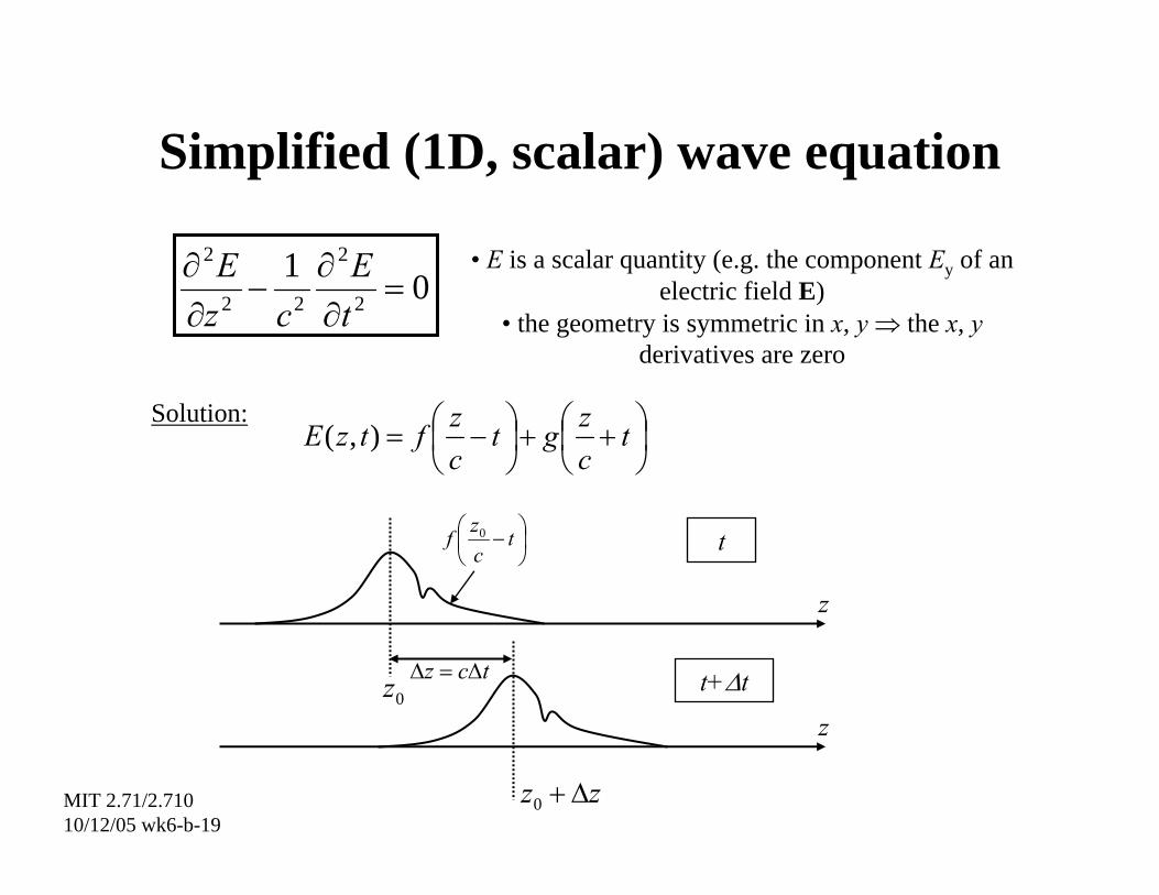
Simplified (1D, scalar) wave equation

012

2

22

2

=∂∂

−∂∂

tE

czE • E is a scalar quantity (e.g. the component Ey of an

electric field E)• the geometry is symmetric in x, y ⇒ the x, y

derivatives are zero

Solution:⎟⎠⎞

⎜⎝⎛ ++⎟

⎠⎞

⎜⎝⎛ −= t

czgt

czftzE ),(

z

z

t

t+∆ttcz ∆=∆0z

zz ∆+0

⎟⎠⎞

⎜⎝⎛ − t

czf 0

MIT 2.71/2.71010/12/05 wk6-b-20

Special case: harmonic solution

λ

z

z

t=0

t+∆t

⎟⎠⎞

⎜⎝⎛==

λπ zatzf 2cos)0,(

( )⎟⎟⎠

⎞⎜⎜⎝

⎛⎟⎠⎞

⎜⎝⎛ −≡⎟

⎠⎞

⎜⎝⎛ −

= tczactzatzf πν

λπ 2cos2cos),( λν=c

dispersionrelationΦ

λπ ct2=∆Φ

MIT 2.71/2.71010/12/05 wk6-b-21

Complex representation of waves

( )

( ) ( )

( ) ( )( ) ( ) ( )

( ) ( ){ }( ) ( ) ( )

phasor""or amplitudecomplex etionrepresenta complex e,ˆ aka ,ˆ

,ˆRe, i.e.

sincos,ˆcos,

2 ,2 cos,

22cos,

φ

φω

φωφω

φω

πνωλπφω

φπνλπ

i

tkzi

AAtzftzf

tzftzf

tkziAtkzAtzf

tkzAtzf

ktkzAtzf

tzAtzf

−

−−=

=

−−+−−=

−−=

==−−=

⎟⎠⎞

⎜⎝⎛ −−=

wave-number

angular frequency

MIT 2.71/2.71010/12/05 wk6-b-22

Time reversal

z

( )uf

( )tkzf ω−

z

( )uf

( )tkzf ω+

MIT 2.71/2.71010/12/05 wk6-b-23

Superposition

z

( )uf

( )tkzf ω−

( )uf

( )tkzf ω+

( ) ( )tkzftkzf ωω ++−⇒ is also a solutionMore generally, ( ) ( )tkzgtkzf ωω ++− is a solution

Even more generally,

( ) ( )( ) ( ) K

K

++++++−+−tkzgtkzg

tkzftkzfωω

ωω

21

21 is a solution

LINEARITY

SUPERPOSITION

MIT 2.71/2.71010/12/05 wk6-b-24

What is the solution to the wave equation?

• In general: the solution is an (arbitrary) superposition of propagating waves

• Usually, we have to impose– initial conditions (as in any differential equation)– boundary condition (as in most partial differential equations)

( ) ( ) ( ) ( )tkzftzfufzf ω−=⇒≡ 0wave0wave ,0,

( ) ( )0,wave0 zfuf =

z

z=0

z

z=0 z=ωt/k

( )tzf ,wave

Example: initial value problem

MIT 2.71/2.71010/12/05 wk6-b-25

What is the solution to the wave equation?

• In general: the solution is an (arbitrary) superposition of propagating waves

• Usually, we have to impose– initial conditions (as in any differential equation)– boundary condition (as in most partial differential equations)

• Boundary conditions: we will not deal much with them in this class, but it is worth noting that physically they explain interesting phenomena such as waveguiding from the wave point of view (we saw already one explanation as TIR).