Smoothed Particle Hydrodynamics (SPH): an Overview … · Smoothed Particle Hydrodynamics (SPH): an...
52
Arch Comput Methods Eng (2010) 17: 25–76 DOI 10.1007/s11831-010-9040-7 Smoothed Particle Hydrodynamics (SPH): an Overview and Recent Developments M.B. Liu · G.R. Liu Received: 1 August 2009 / Accepted: 1 August 2009 / Published online: 13 February 2010 © CIMNE, Barcelona, Spain 2010 Abstract Smoothed particle hydrodynamics (SPH) is a meshfree particle method based on Lagrangian formulation, and has been widely applied to different areas in engineer- ing and science. This paper presents an overview on the SPH method and its recent developments, including (1) the need for meshfree particle methods, and advantages of SPH, (2) approximation schemes of the conventional SPH method and numerical techniques for deriving SPH formulations for partial differential equations such as the Navier-Stokes (N-S) equations, (3) the role of the smoothing kernel func- tions and a general approach to construct smoothing kernel functions, (4) kernel and particle consistency for the SPH method, and approaches for restoring particle consistency, (5) several important numerical aspects, and (6) some recent applications of SPH. The paper ends with some concluding remarks. 1 Introduction 1.1 Traditional Grid Based Numerical Methods Computer simulation has increasingly become a more and more important tool for solving practical and complicated G.R. Liu is SMA Fellow, Singapore-MIT Alliance. M.B. Liu ( ) Key Laboratory for Hydrodynamics and Ocean Engineering, Institute of Mechanics, Chinese Academy of Sciences, #15, Bei Si Huan Xi Road, Beijing 100190, China e-mail: [email protected] G.R. Liu Centre for Advanced Computations in Engineering Science (ACES), Department of Mechanical Engineering, National University of Singapore, 10 Kent Ridge Crescent, Singapore 119260, Singapore problems in engineering and science. It plays a valuable role in providing tests and examinations for theories, offering in- sights to complex physics, and assisting in the interpretation and even the discovery of new phenomena. Grid or mesh based numerical methods such as the finite difference meth- ods (FDM), finite volume methods (FVM) and the finite el- ement methods (FEM) have been widely applied to various areas of computational fluid dynamics (CFD) and compu- tational solid mechanics (CSM). These methods are very useful to solve differential or partial differential equations (PDEs) that govern the concerned physical phenomena. For centuries, the FDM has been used as a major tool for solv- ing partial differential equations defined in problem domains with simple geometries. For decades, the FVM dominates in solving fluid flow problems and FEM plays an essential role for solid mechanics problems with complex geometry [1–3]. One notable feature of the grid based numerical models is to divide a continuum domain into discrete small subdomains, via a process termed as discretization or meshing. The in- dividual grid points (or nodes) are connected together in a pre-defined manner by a topological map, which is termed as a mesh (or grid). The meshing results in elements in FEM, cells in FVM, and grids in FDM. A mesh or grid system consisting of nodes, and cells or elements must be defined to provide the relationship between the nodes before the ap- proximation process for the differential or partial differential equations. Based on a properly pre-defined mesh, the gov- erning equations can be converted to a set of algebraic equa- tions with nodal unknowns for the field variables. So far the grid based numerical models have achieved remarkably, and they are currently the dominant methods in numerical sim- ulations for solving practical problems in engineering and science [1–5]. Despite the great success, grid based numerical methods suffer from difficulties in some aspects, which limit their
Transcript of Smoothed Particle Hydrodynamics (SPH): an Overview … · Smoothed Particle Hydrodynamics (SPH): an...
Arch Comput Methods Eng (2010) 17: 25–76DOI 10.1007/s11831-010-9040-7
Smoothed Particle Hydrodynamics (SPH): an Overviewand Recent Developments
M.B. Liu · G.R. Liu
Received: 1 August 2009 / Accepted: 1 August 2009 / Published online: 13 February 2010© CIMNE, Barcelona, Spain 2010
Abstract Smoothed particle hydrodynamics (SPH) is ameshfree particle method based on Lagrangian formulation,and has been widely applied to different areas in engineer-ing and science. This paper presents an overview on theSPH method and its recent developments, including (1) theneed for meshfree particle methods, and advantages of SPH,(2) approximation schemes of the conventional SPH methodand numerical techniques for deriving SPH formulationsfor partial differential equations such as the Navier-Stokes(N-S) equations, (3) the role of the smoothing kernel func-tions and a general approach to construct smoothing kernelfunctions, (4) kernel and particle consistency for the SPHmethod, and approaches for restoring particle consistency,(5) several important numerical aspects, and (6) some recentapplications of SPH. The paper ends with some concludingremarks.
1 Introduction
1.1 Traditional Grid Based Numerical Methods
Computer simulation has increasingly become a more andmore important tool for solving practical and complicated
G.R. Liu is SMA Fellow, Singapore-MIT Alliance.
M.B. Liu (�)Key Laboratory for Hydrodynamics and Ocean Engineering,Institute of Mechanics, Chinese Academy of Sciences,#15, Bei Si Huan Xi Road, Beijing 100190, Chinae-mail: [email protected]
G.R. LiuCentre for Advanced Computations in Engineering Science(ACES), Department of Mechanical Engineering, NationalUniversity of Singapore, 10 Kent Ridge Crescent, Singapore119260, Singapore
problems in engineering and science. It plays a valuable rolein providing tests and examinations for theories, offering in-sights to complex physics, and assisting in the interpretationand even the discovery of new phenomena. Grid or meshbased numerical methods such as the finite difference meth-ods (FDM), finite volume methods (FVM) and the finite el-ement methods (FEM) have been widely applied to variousareas of computational fluid dynamics (CFD) and compu-tational solid mechanics (CSM). These methods are veryuseful to solve differential or partial differential equations(PDEs) that govern the concerned physical phenomena. Forcenturies, the FDM has been used as a major tool for solv-ing partial differential equations defined in problem domainswith simple geometries. For decades, the FVM dominates insolving fluid flow problems and FEM plays an essential rolefor solid mechanics problems with complex geometry [1–3].One notable feature of the grid based numerical models is todivide a continuum domain into discrete small subdomains,via a process termed as discretization or meshing. The in-dividual grid points (or nodes) are connected together in apre-defined manner by a topological map, which is termedas a mesh (or grid). The meshing results in elements in FEM,cells in FVM, and grids in FDM. A mesh or grid systemconsisting of nodes, and cells or elements must be definedto provide the relationship between the nodes before the ap-proximation process for the differential or partial differentialequations. Based on a properly pre-defined mesh, the gov-erning equations can be converted to a set of algebraic equa-tions with nodal unknowns for the field variables. So far thegrid based numerical models have achieved remarkably, andthey are currently the dominant methods in numerical sim-ulations for solving practical problems in engineering andscience [1–5].
Despite the great success, grid based numerical methodssuffer from difficulties in some aspects, which limit their
26 M.B. Liu, G.R. Liu
applications in many types of complicated problems. Themajor difficulties are resulted from the use of mesh, whichshould always ensure that the numerical compatibility con-dition is the same as the physical compatibility condition fora continuum. Hence, the use of grid/mesh can lead to vari-ous difficulties in dealing with problems with free surface,deformable boundary, moving interface, and extremely largedeformation and crack propagation. Moreover, for problemswith complicated geometry, the generation of a quality meshhas become a difficult, time-consuming and costly process.
In grid based numerical methods, mesh generation for theproblem domain is a prerequisite for the numerical simula-tions. For Eulerian grid methods such as FDM constructinga regular grid for irregular or complex geometry has neverbeen an easy task, and usually requires additional compli-cated mathematical transformation that can be even moreexpensive than solving the problem itself. Determining theprecise locations of the inhomogeneities, free surfaces, de-formable boundaries and moving interfaces within the frameof the fixed Eulerian grid is also a formidable task. TheEulerian methods are also not well suited to problems thatneed monitoring the material properties in fixed volumes,e.g. particulate flows [1, 2, 6]. For the Lagrangian grid meth-ods like FEM, mesh generation is necessary for the solidsand structures, and usually occupies a significant portion ofthe computational effort. Treatment of extremely large de-formation is an important issue in a Lagrangian grid basedmethod. It usually requires special techniques like rezoning.Mesh rezoning, however, is tedious and time-consuming,and may introduce additional inaccuracy into the solution[3, 7].
The difficulties and limitations of the grid based methodsare especially evident when simulating hydrodynamic phe-nomena such as explosion and high velocity impact (HVI).In the whole process of an explosion, there exist specialfeatures such as large deformations, large inhomogeneities,moving material interfaces, deformable boundaries, and freesurfaces [8]. These special features pose great challenges tonumerical simulations using the grid based methods. Highvelocity impact problems involve shock waves propagatingthrough the colliding or impacting bodies that can behavelike fluids. Analytically, the equations of motion and a high-pressure equation of state are the key descriptors of mater-ial behavior. In HVI phenomena, there also exist large de-formations, moving material interfaces, deformable bound-aries, and free surfaces, which are, again, very difficult forgrid based numerical methods to cope with [9].
The grid based numerical methods are also not suitablefor situations where the main concern of the object is a setof discrete physical particles rather than a continuum. Typi-cal examples include the interaction of stars in astrophysics,movement of millions of atoms in an equilibrium or non-equilibrium state, dynamic behavior of protein molecules,
and etc. Simulation of such discrete systems using the con-tinuum grid based methods is often not a good choice [10,11].
1.2 Meshfree Methods
Over the past years, meshfree methods have been a majorresearch focus, towards the next generation of more effec-tive computational methods for more complicated problems[4, 6]. The key idea of the meshfree methods is to provideaccurate and stable numerical solutions for integral equa-tions or PDEs with all kinds of possible boundary condi-tions using a set of arbitrarily distributed nodes or particles[4, 6]. The history, development, theory and applications ofthe major existing meshfree methods have been addressed insome monographs and review articles [4, 6, 7, 12–15]. Thereaders may refer to these literatures for more details of themeshfree methods. To avoid too much detour from our cen-tral topic, this article will not further discuss these meshfreemethods and techniques, except for mentioning briefly someof the latest advancements.
For solid mechanics problems, instead of weak formu-lations used in FEM, we now have a much more powerfulweakened weak (W2) formulation for general settings ofFEM and meshfree methods [16–19]. The W2 formulationcan create various models with special properties, such up-per bound property [20–23], ultra-accurate and supper con-vergent solutions [22, 24–29], and even nearly exact solu-tions [30, 31]. These W2 formulations have a theoreticalfoundation on the novel G space theory [16–19]. All mostall these W2 models work very well with triangular mesh,and applied for adaptive analyses for complicated geome-try.
For fluid dynamics problems, the gradient smoothingmethod (GSM) has been recently formulated using carefullydesigned gradient smoothing domains [32–35]. The GSMworks very well with unstructured triangular mesh, and canbe used effective for adaptive analysis [34]. The GSM is anexcellent alternative to the FVM for CFD problems.
One distinct meshfree method is smoothed particle hy-drodynamics or SPH. The SPH is a very powerful methodfor CFD problems governed by the Navier-Stokes equa-tions.
1.3 Smoothed Particle Hydrodynamics
Smoothed particle hydrodynamics is a “truly” meshfree,particle method originally used for continuum scale appli-cations, and may be regarded as the oldest modern meshfreeparticle method. It was first invented to solve astrophysicalproblems in three-dimensional open space [36, 37], sincethe collective movement of those particles is similar to themovement of a liquid or gas flow, and it can be modeled by
Smoothed Particle Hydrodynamics (SPH): an Overview and Recent Developments 27
the governing equations of the classical Newtonian hydro-dynamics.
In SPH, the state of a system is represented by a setof particles, which possess material properties and interactwith each other within the range controlled by a weight func-tion or smoothing function [6, 38, 39]. The discretization ofthe governing equations is based on these discrete particles,and a variety of particle-based formulations have been usedto calculate the local density, velocity and acceleration of thefluid. The fluid pressure is calculated from the density usingan equation of state, the particle acceleration is then calcu-lated from the pressure gradient and the density. For viscousflows, the effects of physical viscosity on the particle ac-celerations can also be included. As a Lagrangian particlemethod, SPH conserves mass exactly. In SPH, there is noexplicit interface tracking for multiphase flows—the motionof the fluid is represented by the motion of the particles, andfluid surfaces or fluid-fluid interfaces move with particlesrepresenting their phase defined at the initial stage.
SPH has some special advantages over the traditional gridbased numerical methods.
1. SPH is a particle method of Lagrangian nature, and thealgorithm is Galilean invariant. It can obtain the time his-tory of the material particles. The advection and transportof the system can thus be calculated.
2. By properly deploying particles at specific positions atthe initial stage before the analysis, the free surfaces, ma-terial interfaces, and moving boundaries can all be tracednaturally in the process of simulation regardless the com-plicity of the movement of the particles, which have beenvery challenging to many Eulerian methods. Therefore,SPH is an ideal choice for modeling free surface and in-terfacial flow problems.
3. SPH is a particle method without using a grid/mesh.This distinct meshfree feature of the SPH method al-lows a straightforward handling of very large deforma-tions, since the connectivity between particles are gen-erated as part of the computation and can change withtime. Typical examples include the SPH applications inhigh energy phenomena such as explosion, underwaterexplosion, high velocity impact, and penetrations.
4. In SPH method, a particle represents a finite volume incontinuum scale. This is quite similar to the classic mole-cular dynamics (MD) method [11, 40] that uses a particleto represent an atom or a molecule in nano-scale, and thedissipative particle dynamics (DPD) method [41, 42] thatuses a particle to represent a small cluster of moleculesin meso-cale. Thus, it is natural to generalize or extendSPH to smaller scales, or to couple SPH with molecu-lar dynamics and dissipative particle dynamics for multi-ple scale applications, especially in biophysics, and bio-chemistry.
5. SPH is suitable for problems where the object underconsideration is not a continuum. This is especially truein bio- and nano- engineering at micro and nano scale,and astrophysics at astronomic scale. For such problems,SPH can be a natural choice for numerical simulations.
6. SPH is comparatively easier in numerical implementa-tion, and it is more natural to develop three-dimensionalnumerical models than grid based methods.
The early SPH algorithms were derived from the proba-bility theory, and statistical mechanics are extensively usedfor numerical estimation. These algorithms did not conservelinear and angular momentum. However, they can give rea-sonably good results for many astrophysical phenomena.For the simulations of fluid and solid mechanics problems,there are challenges to reproduce faithfully the partial differ-ential equations governing the corresponding fluid and soliddynamics. These challenges involve accuracy and stabilityof the numerical schemes in implementing the SPH meth-ods.
With the development of the SPH method, and the ex-tensive applications to a wide range of problems, more at-tractive features have been showcased while some inher-ent drawbacks have also been identified. Different variantsor modifications have been proposed to improve the orig-inal SPH method. For example, Gingold and Monaghanfound the non-conservation of linear and angular momen-tum of the original SPH algorithm, and then introducedan SPH algorithm that conserves both linear and angularmomentum [43]. Hu and Adams also invented an angular-momentum conservative SPH algorithm for incompressibleviscous flows [44].
Many researchers have conducted investigations on theSPH method on the numerical aspects in accuracy, stabil-ity, convergence and efficiency. Swegle et al. identified thetensile instability problem that can be important for mate-rials with strength [45]. Morris noted the particle inconsis-tency problem that can lead to poor accuracy in the SPHsolution [46]. Over the past years, different modifications orcorrections have been tried to restore the consistency andto improve the accuracy of the SPH method. Monaghanproposed symmetrization formulations that were reportedto have better effects [47–49]. Johnson and his co-workersgave an axis-symmetry normalization formulation so that,for velocity fields that yield constant values of normal ve-locity strains, the normal velocity strains can be exactlyreproduced [50, 51]. Randles and Libersky derived a nor-malization formulation for the density approximation and anormalization for the divergence of the stress tensor [52].Chen et al. proposed a corrective smoothed particle method(CSPM) which improves the simulation accuracy both in-side the problem domain and around the boundary area [53,54]. The CSPM has been improved by Liu et al. in resolv-ing problems with discontinuity such as shock waves in a
28 M.B. Liu, G.R. Liu
discontinuous SPH (DSPH) [55]. Liu et al. also proposeda finite particle method (FPM), which uses a set of basisfunction to approximate field variables at a set of arbitrarilydistributed particles [56, 57]. FPM can be regarded as an im-proved version of SPH and CSPM with better performancein particle consistency. Batra et al. concurrently developed asimilar idea to FPM, and it is named modified SPH (MSPH)[58] with applications mainly in solid mechanics. Fang et al.further improved this idea for simulating free surface flows[59], and they later developed a regularized Lagrangian fi-nite point method for the simulation of incompressible vis-cous flows [60, 61]. A stress point method was invented toimprove the tensile instability and zero energy mode prob-lems [62–65]. Other notable modifications or correctionsof the SPH method include the moving least square parti-cle hydrodynamics (MLSPH) [66, 67], the integration ker-nel correction [68], the reproducing kernel particle method(RKPM) [69, 70], the correction for stable particle method[71, 72], and several other particle consistency restoring ap-proaches [6, 56, 73]. Belytschko and his co-workers haveconducted a series of stability and convergence analyses onmeshfree particle methods, and some of the numerical tech-niques and analyses can also be applicable to SPH [13, 72,74].
This article is organized as follows. In Sect. 1, the back-ground of meshfree particle methods is first addressed withhighlights on overcoming the limitations of the grid basednumerical models. The invention, features and develop-ments of the SPH method are then briefly introduced. InSect. 2, the approximation schemes of the SPH methodare discussed, while some numerical techniques for devel-oping SPH formulations are presented. The SPH formula-tions for the N-S equation, which governs the general fluidflow problems, are also given. Section 3 presents a reviewon the smoothing kernel function. Conditions for construct-ing smoothing functions are developed with examples ofsmoothing functions constructed. Section 4 introduces con-sistency concept of SPH including kernel consistency andparticle consistency, and also provides an in-depth reviewon the existing approaches for restoring particle consistency.Several new approaches are also presented, which include adiscontinuous SPH for simulating problems with disconti-nuity, a general approach to restore particle inconsistency,and a finite particle method. In Sect. 5, some important nu-merical topics in SPH are discussed. These special topicsinclude (1) solid boundary treatment, (2) representation ofsolid obstacles, (3) material interface treatment, and (4) ten-sile instability. Different applications of the SPH methodhave been reviewed in Sect. 6. Some concluding remarksare given in Sect. 7.
2 SPH Approximation Techniques
The conventional SPH method was originally developed forhydrodynamics problems in which the governing equationsare in strong form of partial differential equations of fieldvariables such as density, velocity, energy, and etc. There arebasically two steps in obtaining an SPH formulation. Thefirst step is to represent a function and/or its derivatives incontinuous form as integral representation, and this step isusually termed as kernel approximation. In this kernel ap-proximation step, the approximation of a function and itsderivatives are based on the evaluation of the smoothing ker-nel function and its derivatives. The second step is usuallyreferred to as particle approximation. In this step, the com-putational domain is first discretized by representing the do-main with a set of initial distribution of particles represent-ing the initial settings of the problem. After discretization,field variables on a particle are approximated by a summa-tion of the values over the nearest neighbor particles.
2.1 Kernel Approximation of a Function
The kernel approximation in the SPH method involves rep-resentation of a function and its derivatives using a smooth-ing function. The smoothing function should satisfy somebasic requirements, and it has been called kernel, smoothingkernel, smoothing kernel function, or sometimes even weightfunction in some SPH literature [38, 46, 49, 75]. A detaileddiscussion on smoothing function, basic requirements andconstructing conditions will be given in Sect. 3.
The kernel approximation of a function f (x) used in theSPH method starts from the following identity
f (x) =∫
�
f (x′)δ(x − x′)dx′, (1)
where f is a function of the position vector x, and δ(x −x′)is the Dirac delta function given by
δ(x − x′) ={
1, x = x′,0, x �= x′. (2)
In (1), � is the volume of the integral that contains x. Equa-tion (1) implies that a function can be represented in an inte-gral form. Since the Dirac delta function is used, the integralrepresentation in (2) is exact and rigorous, as long as f (x)
is defined and continuous in �.The Delta function δ(x − x′) with only a “point” sup-
port, and hence (1) cannot be used for establishing discretenumerical models. If replacing the Delta function δ(x − x′)by a smoothing function W(x − x′, h) with a finite spatialdimension h, the kernel approximation of f (x), 〈f (x)〉, be-comes
〈f (x)〉 .=∫
�
f (x′)W(x − x′, h)dx′, (3)
Smoothed Particle Hydrodynamics (SPH): an Overview and Recent Developments 29
where h is the smoothing length defining the influence orsupport area of the smoothing function W . Note that as longas W is not the Dirac delta function, the integral representa-tion shown in (3) can only be an approximation, except forspecial cases. Therefore (3) can be written as
〈f (x)〉 =∫
�
f (x ′)W(x − x′, h)dx′. (4)
A smoothing function W is usually chosen to be an evenfunction for reasons given later in Sect. 3. It should also sat-isfy a number of conditions. The first one is the normaliza-tion condition that states∫
�
W(x − x′, h)dx′ = 1. (5)
This condition is also termed as unity condition since theintegration of the smoothing function produces the unity.
The second condition is the Delta function property thatis observed when the smoothing length approaches zero
limh→0
W(x − x′, h) = δ(x − x′). (6)
The third condition is the compact condition
W(x − x′, h) = 0 when |x − x′| > κh, (7)
where κ is a constant related to the smoothing function for aparticle at x, and κh defines the effective (non-zero) area ofthe smoothing function. This effective area is usually calledas the support domain of the smoothing function for a pointat x (or the support domain of that point). Using this com-pact condition, integration over the entire problem domainis localized as integration over the support domain of thesmoothing function. Therefore, the integration domain �
can be the same as the support domain.In the SPH literatures, the kernel approximation is often
said to have h2 accuracy or second order accuracy [46, 47,49, 75–77]. The observation can be obtained easily usingTaylor series expansion on (4). Note from (7) that the sup-port domain of the smoothing function is |x′ − x| ≤ κh, theerrors in the SPH integral representation can be roughly esti-mated by using the Taylor series expansion of f (x′) aroundx in (4). If f (x) is differentiable, we can get
〈f (x)〉 =∫
�
[f (x) + f ′(x)(x ′ − x) + r((x ′ − x)2)]
× W(x − x′, h)dx′
= f (x)
∫�
W(x − x′, h)dx′ + f ′(x)
∫�
(x′ − x)
× W(x − x′, h)dx′ + r(h2), (8)
where r stands for the residual. Note that W is an even func-tion with respect to x, and (x ′ − x)W(x − x′, h) should bean odd function. Hence we should have∫
�
(x′ − x)W(x − x′, h)dx′ = 0. (9)
Using (5) and (9), (8) becomes
〈f (x)〉 = f (x) + r(h2). (10)
It is clear that SPH kernel approximation of an arbitrary fieldfunction is of second order accuracy.
2.2 Kernel Approximation of Derivatives
The approximation for the spatial derivative ∇ · f (x) is ob-tained simply by substituting f (x) with ∇ · f (x) in (4),which gives
〈∇ · f (x)〉 =∫
�
[∇ · f (x′)]W(x − x′, h)dx′, (11)
where the divergence in the integral is operated with respectto the primed coordinate. Considering
[∇ · f (x′)]W(x − x′, h)
= ∇ · [f (x′)W(x − x′, h)]− f (x′) · ∇[W(x − x′, h)], (12)
the following equation is obtained
∇ · f (x) =∫
�
∇ · [f (x′)W(x − x′, h)]dx′
−∫
�
f (x′) · ∇[W(x − x′, h)]dx′. (13)
The first integral on the right hand side (RHS) of (13) canbe converted using the divergence theorem into an integralover the surface S of the domain of the integration, �, as
〈∇ · f (x)〉 =∫
S
f (x′)W(x − x′, h) · ndS
−∫
�
f (x′) · ∇W(x − x′, h)dx′, (14)
where n is the unit vector normal to the surface S. Since thesmoothing function W is usually defined to have compactsupport (see (7)), the value of W on the surface of the inte-gral in (14) is zero in SPH. Therefore, the surface integralon the right hand side of (14) is also zero. Hence, the kernelapproximation of the derivatives can be written from (14) as
〈∇ · f (x)〉 = −∫
�
f (x′) · ∇W(x − x′, h)dx′. (15)
30 M.B. Liu, G.R. Liu
It is clear that the differential operation on a function istransformed into a differential operation on the smoothingfunction. In other words, the SPH kernel approximation ofthe derivative of a field function allows the spatial gradientto be determined from the values of the function and thederivatives of the smoothing function W , rather than fromthe derivatives of the function itself.
Kernel approximation of higher order derivatives can beobtained in a similar way by substituting f (x) with the cor-responding derivatives in (4), using integration by parts, di-vergence theorem and some trivial transformations. Anotherapproach is to repeatedly use (15) to obtain the kernel ap-proximation of the higher order derivatives, since any higherorder derivative can always be regarded as the first orderderivative of its next lower order derivative.
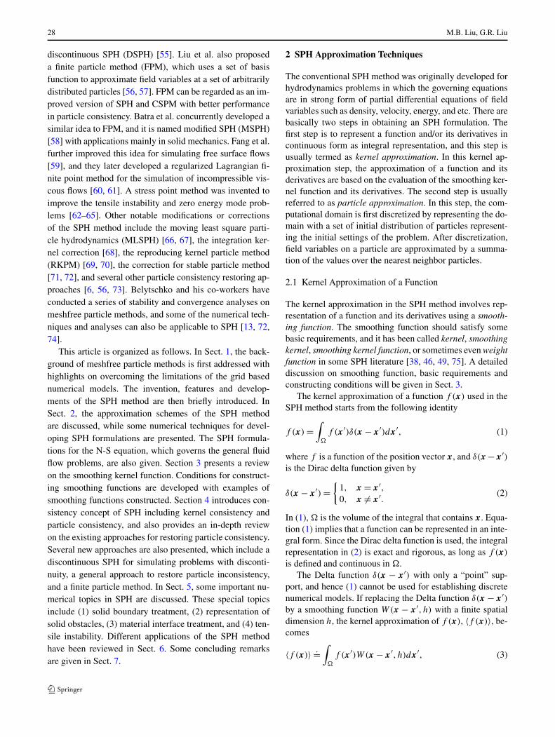
Following similar analyses based on Taylor series expan-sion, it is easy to show that the kernel approximation of thederivative is also of second order accuracy. Since the SPHkernel approximations for a field function and its derivativesare of second order accuracy, that is why the SPH methodhas usually been referred as a method of second order accu-racy. However, (10) is not always true because (5) and (9)are sometimes not satisfied. For example, in a 1D problemspace, if the support domain is within the problem domainunder consideration, the integration of the smoothing func-tion is unity (see (5)), and the integration of the first momentof the smoothing function (see (9)) is zero. Also the sur-face integral in (14) is zero. Hence the SPH kernel approx-imations are of second order accuracy, and this is shown inFig. 1.
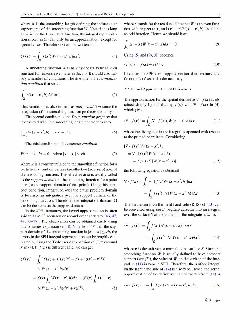
However, there are scenarios in which the support do-main intersects with the problem domain boundary, asshown in Fig. 2. Therefore, the smoothing function W
is truncated by the boundary, and the integration of thesmoothing function is no longer unity. The integration of thefirst moment term of the smoothing function and the surfaceintegral in (14) are also no longer zero. At such scenarios,the SPH kernel approximations are not of second order ac-curacy.
2.3 Particle Approximation
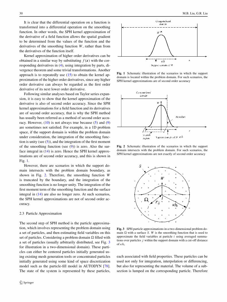
The second step of SPH method is the particle approxima-tion, which involves representing the problem domain usinga set of particles, and then estimating field variables on thisset of particles. Considering a problem domain � filled witha set of particles (usually arbitrarily distributed, see Fig. 3for illustration in a two-dimensional domain). These parti-cles can either be centered particles initially generated us-ing existing mesh generation tools or concentrated particlesinitially generated using some kind of space discretizationmodel such as the particle-fill model in AUTODYN [78].The state of the system is represented by these particles,
Fig. 1 Schematic illustration of the scenarios in which the supportdomain is located within the problem domain. For such scenarios, theSPH kernel approximations are of second order accuracy
Fig. 2 Schematic illustration of the scenarios in which the supportdomain intersects with the problem domain. For such scenarios, theSPH kernel approximations are not exactly of second order accuracy
Fig. 3 SPH particle approximations in a two-dimensional problem do-main � with a surface S. W is the smoothing function that is used toapproximate the field variables at particle i using averaged summa-tions over particles j within the support domain with a cut-off distanceof κhi
each associated with field properties. These particles can beused not only for integration, interpolation or differencing,but also for representing the material. The volume of a sub-section is lumped on the corresponding particle. Therefore
Smoothed Particle Hydrodynamics (SPH): an Overview and Recent Developments 31
one particle i is associated with a fixed lumped volume �Vi
without fixed shape. If the particle mass and density are con-cerned, the lumped volume can also be replaced with thecorresponding mass to density ratio mi/ρi . These particlescan be fixed in an Eulerian frame or move in a Lagrangianframe.
After representing the computational domain with a finitenumber of particles, the continuous form of kernel approx-imation expressed in (4) can be written in discretized formof a summation of the neighboring particles as follows
〈f (x)〉 =N∑
j=1
mj
ρj
f (xj )W(x − xj , h), (16)
where N is the total number of particles within the influencearea of the particle at x. It is the total number of particlesthat are within the support domain which has a cut-off dis-tance, characterized by the smoothing length, h, multipliedby a scalar constant κ . This procedure of summation over theneighboring particles is referred to as particle approxima-tion, which states that the value of a function at a particle canbe approximated by using the average of the values of thefunction at all the particles in the support domain weightedby the smoothing function. Following the same procedure,the particle approximation of a derivative can be obtained as
〈∇ · f (x)〉 = −N∑
j=1
mj
ρj
f (xj ) · ∇W(x − xj , h), (17)
where the gradient ∇W in the above equation is evaluated atparticle j . Equation (17) states that the value of the gradientof a function at a particle located at x can be approximatedby using the summation of those values of the function atall the particles in the support domain weighted by the gra-dient of the smoothing function. The particle approximationin (16) and (17) converts the continuous form of kernel ap-proximation of a field function and its derivatives to the dis-crete summations over a set of particles. The use of parti-cle summations to approximate the integral is, in fact, a keyapproximation that makes the SPH method simple withoutusing a background mesh for numerical integration, and it isalso the key factor influencing the solution accuracy of theSPH method.
One important aspect is that the particle approximationin the SPH method introduces the mass and density of theparticle into the equations. This can be conveniently ap-plied to hydrodynamic problems in which the density is akey field variable. This is probably one of the major reasonsfor the SPH method being particularly popular for dynamicfluid flow problems. If the SPH particle approximation isapplied to solid mechanics problems, special treatments arerequired. One of the ways is to use the SPH approximationto create shape functions, and to establish the discrete sys-tem equations [4].
The particle approximation is, however, related to somenumerical problems inherent in the SPH method, such asthe particle inconsistency and the tensile instability, as willbe addressed in the following sections. One basic reasonis that the discrete summation is only taken over the parti-cles themselves (collocation). In general, in meshfree meth-ods, to achieve stability and accuracy, the number of sam-pling points for integration should be more than the fieldnodes (particles). This is especially true for meshfree meth-ods based on weak forms for solid mechanics problems [4].Otherwise, it may (not always) lead to some kind of insta-bility problems.
2.4 Techniques for Deriving SPH Formulations
By using the above-described procedure of kernel approx-imation and particle approximation, SPH formulations forpartial differential equations can always be derived. Thereare in fact a number of ways to derive SPH formulation ofPDEs. Benz used one approach to derive the SPH equationsfor PDEs that is to multiply each term in the PDEs with thesmoothing function, and integrate over the volume with theuse of integration by parts and Taylor expansions [79]. Mon-aghan employed a straightforward approach of directly us-ing (16) and (17) [49]. In that approach, the following twoidentities are employed to place the density inside the gradi-ent operator,
∇ · f (x) = 1
ρ[∇ · (ρf (x)) − f (x) · ∇ρ], (18)
∇ · f (x) = ρ
[∇ ·
(f (x)
ρ
)+ f (x)
ρ2· ∇ρ
]. (19)
The above two identities may be substituted into the integralin (11). The same procedure of the particle approximationto obtain (17) is applied to each gradient term on the righthand side of (18) and (19). Note that each expression at theoutside of every gradient term is evaluated at the particleitself, the results from (18) and (19) for the divergence off (x) at particle i are obtained as
〈∇ · f (xi )〉 = 1
ρi
[N∑
j=1
mj [f (xj ) − f (xi )] · ∇iWij
], (20)
and
〈∇ · f (xi )〉
= ρi
[N∑
j=1
mj
[(f (xj )
ρ2j
)+
(f (xi )
ρ2i
)]· ∇iWij
]. (21)
One of the good features for the above two equations isthat the field function f (x) appears pairwisely and involves
32 M.B. Liu, G.R. Liu
asymmetric and symmetric SPH formulations. These asym-metric and symmetric formulations can help to improve thenumerical accuracy in SPH simulations [6, 49, 56].
Besides the above-mentioned two identities, some otherrules of operation can be convenient in deriving the SPHformulations for complex system equations [6]. For exam-ple, for two arbitrary functions of field variables f1 and f2,the following rules exist.
〈f1 ± f2〉 = 〈f1〉 ± 〈f2〉, (22)
〈f1f2〉 = 〈f1〉〈f2〉. (23)
Hence, an SPH approximation of the sum of functionsequals to the sum of the SPH approximations of the indi-vidual function, and an SPH approximation of a product offunctions equals to the product of the SPH approximationsof the individual functions.
If f1 is a constant denoted by c, we should have
〈cf2〉 = c〈f2〉. (24)
It is clear that the SPH approximation operator is a linearoperator. It is also easy to show that the SPH approximationoperator is commutative, i.e.,
〈f1 + f2〉 = 〈f2 + f1〉, (25)
and
〈f1f2〉 = 〈f2f1〉. (26)
For convenience, the SPH approximation operator “〈 〉” isomitted in later sections.
2.5 SPH Formulations for Navier-Stokes (N-S) Equations
Using the afore-mentioned kernel and particle approxima-tion techniques with necessary numerical tricks, it is possi-ble to derive SPH formulations for partial differential equa-tions governing the physics of fluid flows. For example, forNavier-Stokes equations controlling the general fluid dy-namic problems, we have⎧⎪⎪⎪⎨⎪⎪⎪⎩
DρDt
= −ρ ∂vβ
∂xβ ,
Dvα
Dt= 1
ρ∂σαβ
∂xβ + F,
DeDt
= σαβ
ρ∂vα
∂xβ ,
(27)
where the Greek superscripts α and β are used to denotethe coordinate directions, the summation in the equations istaken over repeated indices, and the total time derivatives aretaken in the moving Lagrangian frame. The scalar densityρ, and internal energy e, the velocity component vα , andthe total stress tensor σαβ are the dependent variables. F isthe external forces such as gravity. The spatial coordinates
xα and time t are the independent variables. The total stresstensor σαβ is made up of two parts, one part of isotropicpressure p and the other part of viscous stress τ , i.e., σαβ =−pδαβ +ταβ . For Newtonian fluids, the viscous shear stressshould be proportional to the shear strain rate denoted by ε
through the dynamic viscosity μ, i.e., ταβ = μεαβ , where
εαβ = ∂vβ
∂xα+ ∂vα
∂xβ− 2
3(∇ · v)δαβ.
Substituting the SPH approximations for a function andits derivative (as shown in (16) and (17)) to the N-S equa-tions, the SPH equations of motion for the N-S equationscan be written as⎧⎪⎪⎪⎪⎪⎪⎨⎪⎪⎪⎪⎪⎪⎩
Dρi
Dt= ∑N
j=1 mjvβij
∂Wij
∂xβi
,
Dvαi
Dt= −∑N
j=1 mj
(σ
αβi
ρ2i
+ σαβj
ρ2j
)∂Wij
∂xβi
+ Fi,
Dei
Dt= 1
2
∑Nj=1 mj
(pi
ρ2i
+ pj
ρ2j
)v
βij
∂Wij
∂xβi
+ μi
2ρiεαβi ε
αβi ,
(28)
where vij = vi − vj . Equation (28) is a set of commonlyused SPH equations for the N-S equations. It should benoted that by using different numerical tricks, it is possi-ble to get other different forms of SPH equations for thesame partial differential equations. The obtained SPH for-mulations may have special features and advantages suitablefor different applications [6]. One typical example is the ap-proximation of density. If the field function is the density,(16) can be re-written as
ρi =N∑
j=1
mjWij . (29)
This is another approach to obtain density directly from theSPH summation of the mass of all particles in the supportdomain of a given particle, rather than from the continuumequation. Compared to the SPH formulations on densitychange in (28), this summation density approach conservesmass exactly, but suffers from serious boundaries deficiencydue to the particle inconsistency. A frequently used way toremediate the boundaries deficiency is the following normal-ization form by the summation of the smoothing functionitself [52, 53]
ρi =∑N
j=1 mjWij∑Nj=1(
mj
ρj)Wij
. (30)
3 SPH Smoothing Function
3.1 Review on Commonly Used Smoothing Functions
One of the central issues for meshfree methods is how to ef-fectively perform function approximation based on a set of
Smoothed Particle Hydrodynamics (SPH): an Overview and Recent Developments 33
nodes scattered in an arbitrary manner without using a pre-defined mesh or grid that provides the connectivity of thenodes. In the SPH method, the smoothing function is usedfor kernel and particle approximations. It is of utmost im-portance in the SPH method as it determines the pattern tointerpolate, and defines the cut-off distance of the influenc-ing area of a particle.
Many researchers have investigated the smoothing ker-nel, hoping to improve the performance of the SPH method,and/or to generalize the requirements for constructing thesmoothing kernel function. Fulk numerically investigated anumber of smoothing kernel functions in one-dimensionalspace, and the obtained results are basically valid for regu-larly distributed particles [39, 75]. Swegle et al. revealed thetensile instability, which is closely related to the smooth-ing kernel function [45]. Morris studied the performancesof several different smoothing functions, and found that byproperly selecting the smoothing function, the accuracy andstability property of the SPH simulation can be improved[46, 80]. Omang provided investigations on alternative ker-nel functions for SPH in cylindrical symmetry [81]. Jin andDing investigated the criterions for smoothed particle hy-drodynamics kernels in stable field [82]. Capuzzo-Dolcettagave a criterion for the choice of the interpolation ker-nel in SPH [83]. Cabezon and his co-workers proposed aone-parameter family of interpolating kernels for SPH stud-ies [84].
Different smoothing functions have been used in the SPHmethod as shown in published literatures. Various require-ments or properties for the smoothing functions have beendiscussed. Major properties or requirements are now sum-marized and described in the following discussion.
1. The smoothing function must be normalized over its sup-port domain (Unity)∫
�
W(x − x′, h)dx′ = 1. (31)
This normalization property ensures that the integral ofthe smoothing function over the support domain to beunity. It can be shown in the next section that it also en-sures the zero-th order consistency (C0) of the integralrepresentation of a continuum function.
2. The smoothing function should be compactly supported(Compact support), i.e.,
W(x − x′) = 0, for |x − x′| > κh. (32)
The dimension of the compact support is defined by thesmoothing length h and a scaling factor κ , where h isthe smoothing length, and κ determines the spread of thespecified smoothing function. |x − x′| ≤ κh defines thesupport domain of the particle at point x. This compactsupportness property transforms an SPH approximation
from a global operation to a local operation. This willlater lead to a set of sparse discretized system matrices,and therefore is very important as far as the computa-tional efforts are concerned.
3. W(x − x′) ≥ 0 for any point at x′ within the support do-main of the particle at point x (Positivity). This propertystates that the smoothing function should be non-negativein the support domain. It is not mathematically necessaryas a convergent condition, but it is important to ensurea meaningful (or stable) representation of some physi-cal phenomena. A few smoothing functions used in someliteratures are negative in parts of the support domain.However in hydrodynamic simulations, negative value ofthe smoothing function can have serious consequencesthat may result in some unphysical parameters such asnegative density and energy.
4. The smoothing function value for a particle should bemonotonically decreasing with the increase of the dis-tance away from the particle (Decay). This property isbased on the physical consideration in that a nearer par-ticle should have a bigger influence on the particle underconsideration. In other words, with the increase of thedistance of two interacting particles, the interaction forcedecreases.
5. The smoothing function should satisfy the Dirac deltafunction condition as the smoothing length approacheszero (Delta function property)
limh→0
W(x − x′, h) = δ(x − x′). (33)
This property makes sure that as the smoothing lengthtends to be zero, the approximation value approaches thefunction value, i.e. 〈f (x)〉 = f (x).
6. The smoothing function should be an even function(Symmetric property). This means that particles fromsame distance but different positions should have equaleffect on a given particle. This is not a very rigid condi-tion, and it is sometimes violated in some meshfree par-ticle methods that provide higher consistency.
7. The smoothing function should be sufficiently smooth(Smoothness). This property aims to obtain better ap-proximation accuracy. For the approximations of a func-tion and its derivatives, a smoothing function needs to besufficiently continuous to obtain good results. A smooth-ing function with smoother value of the function andderivatives would usually yield better results and betterperformance in numerical stability. This is because thesmoothing function will not be sensitive to particle dis-order, and the errors in approximating the integral inter-polants are small, provided that the particle disorder isnot extreme [6, 49, 75].
Any function having the above properties may be em-ployed as SPH smoothing functions, and many kinds of
34 M.B. Liu, G.R. Liu
smoothing functions have been used. Lucy in the originalSPH paper [36] used a bell-shaped function
W(x − x′, h) = W(R,h)
= αd
{(1 + 3R)(1 − R)3, R ≤ 1,
0, R > 1,(34)
where αd is 5/4h, 5/πh2 and 105/16πh3 in one-, two- andthree-dimensional space, respectively, so that the conditionof unity can be satisfied for all the three dimensions. R isthe relative distance between two points (particles) at pointsx and x′, R = r
h= |x−x′|
h, where r is the distance between
the two points.Gingold and Monaghan in their original paper [37] se-
lected the following Gaussian kernel to simulate the non-spherical stars
W(R,h) = αde−R2, (35)
where αd is 1/π1/2h, 1/πh2 and 1/π3/2h3, respectively,in one-, two- and three-dimensional space, for the unityrequirement. The Gaussian kernel is sufficiently smootheven for high orders of derivatives, and is regarded as a“golden” selection since it is very stable and accurate es-pecially for disordered particles. It is, however, not reallycompact, as it never goes to zero theoretically, unless R ap-proaches infinity. Because it approaches zero numericallyvery fast, it is practically compact. Note that it is computa-tionally more expensive since it can take a longer distancefor the kernel to approach zero. This can result in a largesupport domain with more particles for particle approxima-tions.
The most frequently used smoothing function may be thecubic B-spline function, which was originally used by Mon-aghan and Lattanzio [85]
W(R,h) = αd ×
⎧⎪⎨⎪⎩
23 − R2 + 1
2R3, 0 ≤ R < 1,16 (2 − R)3, 1 ≤ R < 2,
0, R ≥ 2.
(36)
In one-, two- and three-dimensional space, αd = 1/h,15/7πh2 and 3/2πh3, respectively. The cubic spline func-tion has been the most widely used smoothing function inthe emerged SPH literatures since it closely resembles aGaussian function while having a narrower compact sup-port. However, the second derivative of the cubic spline isa piecewise linear function, and accordingly, the stabilityproperties can be inferior to those of smoother kernels.
Morris has introduced higher order (quartic and quintic)splines that are more closely approximating the Gaussianand more stable [46, 80]. The quartic spline is
W(R,h)
= αd ×
⎧⎪⎪⎪⎪⎪⎪⎪⎨⎪⎪⎪⎪⎪⎪⎪⎩
(R + 2.5)4 − 5(R + 1.5)4 + 10(R + 0.5)4,
0 ≤ R < 0.5,
(2.5 − R)4 − 5(1.5 − R)4,
0.5 ≤ R < 1.5,
(2.5 − R)4, 1.5 ≤ R < 2.5,
0, R > 2.5,
(37)
where αd is 1/24h in one-dimensional space. The quinticspline is
W(R,h) = αd ×
⎧⎪⎪⎪⎪⎪⎪⎪⎨⎪⎪⎪⎪⎪⎪⎪⎩
(3 − R)5 − 6(2 − R)5 + 15(1 − R)5,
0 ≤ R < 1,
(3 − R)5 − 6(2 − R)5,
1 ≤ R < 2,
(3 − R)5, 2 ≤ R < 3,
0, R > 3,
(38)
where αd is 120/h, 7/478πh2 and 3/359πh3 in one-, two-and three-dimensional space, respectively.
Johnson et al. used the following quadratic smoothingfunction to simulate high velocity impact problems [86]
W(R,h) = αd
(3
16R2 − 3
4R + 3
4
), 0 ≤ R ≤ 2, (39)
where in one-, two- and three-dimensional space, αd = 1/h,2/πh2 and 5/4πh3, respectively. Unlike other smoothingfunctions, the derivative of this quadratic smoothing func-tion always increases as the particles move closer, and al-ways decreases as they move apart. This was regarded by theauthors as an important improvement over the cubic splinefunction, and it was reported to relieve the problem of com-pressive instability.
Some higher order smoothing functions that are devisedfrom lower order forms have been constructed, such as thesuper-Gaussian kernel [85]
W(R,h) = αd
(3
2− R2
)e−R2
, 0 ≤ R ≤ 2, (40)
where αd is 1/√
π in one-dimensional space. One disadvan-tage of the high order smoothing function is that the kernelis negative in some region of its support domain. This maylead to unphysical results for hydrodynamic problems [75].
The smoothing function has been studied mathematicallyin detail by Liu and his co-workers. They proposed a system-atical way to construct a smoothing function that may meetdifferent needs [38]. A new quartic smoothing function hasbeen constructed to demonstrate the effectiveness of the ap-proach for constructing a smoothing function as follows.
W(R,h) = αd
{( 2
3 − 98R2 + 19
24R3 − 532R4), 0 ≤ R ≤ 2,
0, R > 2,(41)
Smoothed Particle Hydrodynamics (SPH): an Overview and Recent Developments 35
where αd is 1/h, 15/7πh2 and 315/208πh3 in one-, two-and three-dimensional space, respectively. Note that the cen-tre peak value of this quartic smoothing function is definedas 2/3. The quartic smoothing function behaves very muchlike the widely used cubic B-spline function given in (36),but has only one piece, and hence is much more conve-nient and efficient to use. More discussions on this quarticsmoothing function will give in the next section.
3.2 Generalizing Constructing Conditions
Major requirements of an SPH smoothing function havebeen addressed in Sect. 3.1. Some of these requirements canbe derived by conducting Taylor series analysis. This analy-sis is carried out at the stage of the SPH kernel approxi-mation for a function and its derivatives. It shows that, toexactly approximate a function and its derivatives, certainconditions need to be satisfied. These conditions can then beused to construct the smoothing functions.
Considering the SPH kernel approximation for a fieldfunction f (x) as show in (4), if f (x) is sufficiently smooth,applying Taylor series expansion of f (x′) in the vicinity ofx yields
f (x′) = f (x) + f ′(x)(x ′ − x) + 1
2f ′′(x)(x ′ − x)2 + · · ·
=n∑
k=0
(−1)khkf (k)(x)
k!(
x − x′
h
)k
+ rn
(x − x′
h
), (42)
where rn is the remainder of the Taylor series expansion.Substituting (42) into (4) leads to
f (x) =n∑
k=0
Akf(k)(x) + rn
(x − x′
h
), (43)
where
Ak = (−1)khk
k!∫
�
(x − x′
h
)k
W(x − x′, h)dx′. (44)
Comparing the LHS with the RHS of (43), in order forf (x) to be approximated to n-th order, the coefficients Ak
must equal to the counterparts for f (k)(x) at the LHS of(43). Therefore, after trivil transformation, the followingconditions for the smoothing function W can be obtainedas follows
M0 = ∫�
W(x − x′, h)dx′ = 1
M1 = ∫�(x − x′)W(x − x′, h)dx′ = 0
M2 = ∫�(x − x′)2W(x − x′, h)dx′ = 0
...
Mn = ∫�(x − x′)nW(x − x′, h)dx′ = 0
⎫⎪⎪⎪⎪⎪⎪⎬⎪⎪⎪⎪⎪⎪⎭
, (45)
where Mk is the k-th moments of the smoothing function.Note that the first equation in (45) is, in fact, the unity con-dition expressed in (31), and the second equation in (45)stands for the symmetric property. Satisfaction of these twoconditions ensures the first order consistency for the SPHkernel approximation for a function.
Also performing Taylor series analysis for the SPH ker-nel approximation of the derivatives of a field function f (x),using the concept of integration by parts, and divergence the-orem with some trivial transformation, the following equa-tions
W(x − x′, h)|S = 0 (46)
and
M ′0 = ∫
�W ′(x − x′, h)dx′ = 0
M ′1 = ∫
�(x − x′)W ′(x − x′, h)dx′ = 1
M ′2 = ∫
�(x − x′)2W ′(x − x′, h)dx′ = 0
...
M ′n = ∫
�(x − x′)nW ′(x − x′, h)dx′ = 0
⎫⎪⎪⎪⎪⎪⎪⎬⎪⎪⎪⎪⎪⎪⎭
(47)
can be obtained. Equation (46) actually specifies that thesmoothing function vanishes on the surface of the supportdomain. This is compatible to the compactness condition ofthe smoothing function. Equation (47) defines the conditionswith which the derivatives of the smoothing function shouldbe satisfied. Note that (45) and (47) are actually compatibleconsidering integration by parts, divergence theorem and theboundary value vanishing effects (see (46)) of the smoothingfunction.
Performing Taylor series analysis on the SPH kernel ap-proximation for the second derivatives, similar equationscan be obtained. Except for the requirements on the sec-ond derivatives of the momentums, the first derivative ofthe smoothing function also needs to vanish on the surface,which is
W ′(x − x′, h)|S = 0. (48)
Equations (45)–(48) can be used to construct smoothingfunctions. It can be seen that the conditions of smoothingfunctions can be classified into two groups. The first groupshows the ability of a smoothing function to reproduce poly-nomials. Satisfying the first group, the function can be ap-proximated to n-th order accuracy. The second group definesthe surface values of a smoothing function as well as its firstderivatives, and is the requirements of the property of com-pact support for the smoothing function and its first deriva-tive. Satisfying these conditions, the first two derivatives ofthe function can be exactly approximated to the n-th order.
36 M.B. Liu, G.R. Liu
3.3 Constructing SPH Smoothing Functions
By using above-mentioned conditions, it is possible to havea systematic way to construct the SPH smoothing functions.If the smoothing function is assumed to be a polynomialdependent only on the relative distance of the concernedpoints, it can be assumed to have the following form in thesupport domain with an influence width of κh.
W(x − x′, h) = W(R) = a0 + a1R + a2R2 + · · · + anR
n.
(49)
It is clear that a smoothing function in the above-mentioned form is a distance function since it depends on therelative distance. It is easy to show that for the second deriv-ative of the smoothing function to exist, a1 should vanish.Substituting this polynomial form smoothing function intothe conditions (see (45)–(48)), the parameters a0, a2, . . . , an
can be calculated from the resultant linear equations, andthen the smoothing function can be determined.
There are several issues that need further consideration.Firstly, a smoothing function derived from this set of condi-tions (see (45)) will not necessarily be positive in the entiresupport domain, especially when high order reproducibil-ity is required. Such a negative smoothing function may re-sult in unphysical solutions, for example, negative density(mass) and negative energy. For this reason, smoothing func-tions used in SPH literatures are generally non-negative forCFD problems. On the other hand, for the even moments(k = 2,4,6, . . .) to be zero, a smoothing function has tobe negative in some parts of the region. This implies thatone cannot have both non-negativity and high-order repro-ducibility at the same time.
Secondly, in constructing a smoothing function, the cen-ter peak value is a factor that needs to be considered. Thecenter peak value of a smoothing function is very importantsince it determines how much the particle itself will con-tribute to the approximation. Revisiting (45), if a positivesmoothing function is used, the highest order of accuracyfor the function approximation is second order. Therefore,the second momentum (M2 = ∫
�(x −x′)2W(x −x′, h)dx′)
can be used as a rough indicator to measure the accuracyof the kernel approximation. The smaller the second mo-ment M2 is, the more accurate the kernel approximation is.The center peak value of a smoothing function is closelyrelated to M2. A positive smoothing function with a largecenter peak value will have a smaller second moment M2.This implies that a smoothing function is closer to the Deltafunction, and therefore is more accurate in terms of kernelapproximations.
Thirdly, in some circumstances, a piecewise smooth-ing function is preferable since the shape of the piecewisesmoothing function is easier to be controlled by changing
the number of the pieces and the locations of the connectionpoints. For example, consider the general form of a smooth-ing function with two pieces,
W(R) =⎧⎨⎩
W1(R), 0 ≤ R < R1,W2(R), R1 ≤ R < R2,0 R2 ≤ R.
(50)
The function itself and the first two derivatives at theconnection points should be continuous, i.e., W1(R1) =W2(R1), W ′
1(R1) = W ′2(R1) and W ′′
1 (R1) = W ′′2 (R1). Con-
sidering the requirements at these points as well as the com-pact support property, one possible form of the smoothingfunction is
W(R) = αd
⎧⎨⎩
b1(R1 − R)n + b2(R2 − R)n, 0 ≤ R < R1,
b2(R2 − R)n, R1 ≤ R < R2,
0, R2 ≤ R.
(51)
It is also feasible to construct smoothing function with morepieces using similar expressions.
To show the effectiveness of this approach to construct-ing general SPH smoothing functions Liu et al. [38] deriveda new quartic smoothing function using the following con-ditions
• the unity condition,• compact support of the smoothing function,• compact support of the first derivative of the smoothing
function,• centre peak value.
The constructed smoothing function is given as W(R,h) =αd( 2
3 − 98R2 + 19
24R3 − 532R4), for 0 ≤ R ≤ 2, where αd is
1/h, 15/7πh2 and 315/208πh3 in one-, two- and three-dimensional space, respectively. Note that the centre peakvalue of this quartic smoothing function is defined as 2/3.
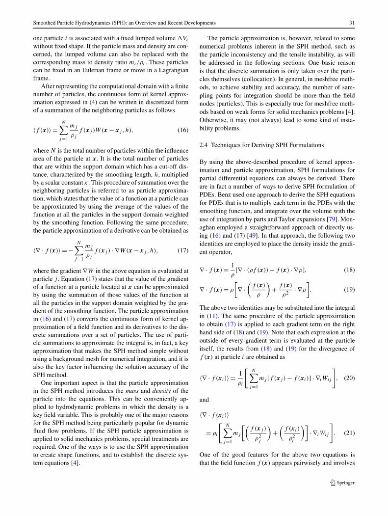
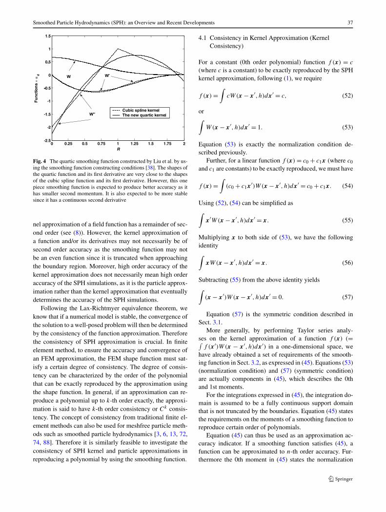
As defined, this quartic function satisfies the normaliza-tion condition, while the function itself and its first deriva-tive have compact support. It is very close to the most com-monly used cubic spline (see (36)) with a same center peakvalue of 2/3, and monotonically decreases with the increaseof the distance as show in Fig. 4. However, this quartic func-tion produces a smaller second momentum than the cubicspline function, and therefore can produce better accuracyfor kernel approximation. Also this quartic smoothing func-tion has a smoother second derivative than the cubic splinesmoothing function, thus the stability properties should besuperior to those of the cubic spline function, as reported bymany researchers that a smoother second derivative can leadto less instability in SPH simulation [80, 87].
4 Consistency
In early studies, the SPH method has usually been reportedto have second order accuracy. This is reasonable, as the ker-
Smoothed Particle Hydrodynamics (SPH): an Overview and Recent Developments 37
Fig. 4 The quartic smoothing function constructed by Liu et al. by us-ing the smoothing function constructing conditions [38]. The shapes ofthe quartic function and its first derivative are very close to the shapesof the cubic spline function and its first derivative. However, this onepiece smoothing function is expected to produce better accuracy as ithas smaller second momentum. It is also expected to be more stablesince it has a continuous second derivative
nel approximation of a field function has a remainder of sec-ond order (see (8)). However, the kernel approximation ofa function and/or its derivatives may not necessarily be ofsecond order accuracy as the smoothing function may notbe an even function since it is truncated when approachingthe boundary region. Moreover, high order accuracy of thekernel approximation does not necessarily mean high orderaccuracy of the SPH simulations, as it is the particle approx-imation rather than the kernel approximation that eventuallydetermines the accuracy of the SPH simulations.
Following the Lax-Richtmyer equivalence theorem, weknow that if a numerical model is stable, the convergence ofthe solution to a well-posed problem will then be determinedby the consistency of the function approximation. Thereforethe consistency of SPH approximation is crucial. In finiteelement method, to ensure the accuracy and convergence ofan FEM approximation, the FEM shape function must sat-isfy a certain degree of consistency. The degree of consis-tency can be characterized by the order of the polynomialthat can be exactly reproduced by the approximation usingthe shape function. In general, if an approximation can re-produce a polynomial up to k-th order exactly, the approxi-mation is said to have k-th order consistency or Ck consis-tency. The concept of consistency from traditional finite el-ement methods can also be used for meshfree particle meth-ods such as smoothed particle hydrodynamics [3, 6, 13, 72,74, 88]. Therefore it is similarly feasible to investigate theconsistency of SPH kernel and particle approximations inreproducing a polynomial by using the smoothing function.
4.1 Consistency in Kernel Approximation (KernelConsistency)
For a constant (0th order polynomial) function f (x) = c
(where c is a constant) to be exactly reproduced by the SPHkernel approximation, following (1), we require
f (x) =∫
cW(x − x′, h)dx′ = c, (52)
or∫
W(x − x′, h)dx′ = 1. (53)
Equation (53) is exactly the normalization condition de-scribed previously.
Further, for a linear function f (x) = c0 + c1x (where c0
and c1 are constants) to be exactly reproduced, we must have
f (x) =∫
(c0 + c1x′)W(x − x′, h)dx′ = c0 + c1x. (54)
Using (52), (54) can be simplified as∫
x′W(x − x′, h)dx′ = x. (55)
Multiplying x to both side of (53), we have the followingidentity∫
xW(x − x′, h)dx′ = x. (56)
Subtracting (55) from the above identity yields∫
(x − x′)W(x − x′, h)dx′ = 0. (57)
Equation (57) is the symmetric condition described inSect. 3.1.
More generally, by performing Taylor series analy-ses on the kernel approximation of a function f (x) (=∫
f (x′)W(x − x′, h)dx′) in a one-dimensional space, wehave already obtained a set of requirements of the smooth-ing function in Sect. 3.2, as expressed in (45). Equations (53)(normalization condition) and (57) (symmetric condition)are actually components in (45), which describes the 0thand 1st moments.
For the integrations expressed in (45), the integration do-main is assumed to be a fully continuous support domainthat is not truncated by the boundaries. Equation (45) statesthe requirements on the moments of a smoothing function toreproduce certain order of polynomials.
Equation (45) can thus be used as an approximation ac-curacy indicator. If a smoothing function satisfies (45), afunction can be approximated to n-th order accuracy. Fur-thermore the 0th moment in (45) states the normalization
38 M.B. Liu, G.R. Liu
condition, and the 1st moment states the symmetry propertyof the smoothing function.
Similar to the consistency concept in the traditional FEM,if an SPH approximation can reproduce a polynomial of upto nth order exactly, the SPH approximation is said to haventh order or Cn consistency. If the consistency of an SPHkernel approximation in continuous form is termed as ker-nel consistency, the kernel consistency of an SPH kernel ap-proximation is of nth order when the smoothing functionsatisfies (45). Therefore the expressions in (45) are also thekernel consistency conditions of the smoothing function foran SPH kernel approximation.
Note that if the SPH kernel approximations are carriedout for regions truncated by boundaries, constant and lin-ear functions can not be reproduced exactly since (53) and(57) are not satisfied for these regions. Therefore we canconclude that, since a conventional smoothing function sat-isfies the normalization and symmetric conditions, the con-ventional SPH method has up to C1 consistency for the inte-rior regions. However, for the boundary regions, it even doesnot have C0 kernel consistency.
4.2 Consistency in Particle Approximation (ParticleConsistency)
Satisfying the consistency conditions at the kernel approxi-mation stage does not necessarily mean that the discretizedSPH model will have such a consistency. This is becausesuch a consistency can be distorted by the particle approxi-mation process in discrete SPH model. Therefore, the con-sistency analysis should be conducted for the discrete SPHmodel in the particle approximation process, and this con-sistency can be termed as particle consistency.
The discrete counterparts of the constant and linear con-sistency conditions as expressed in (53) and (57) are
N∑j=1
W(x − xj , h)�vj = 1, (58)
and
N∑j=1
(x − xj )W(x − xj , h)�vj = 0. (59)
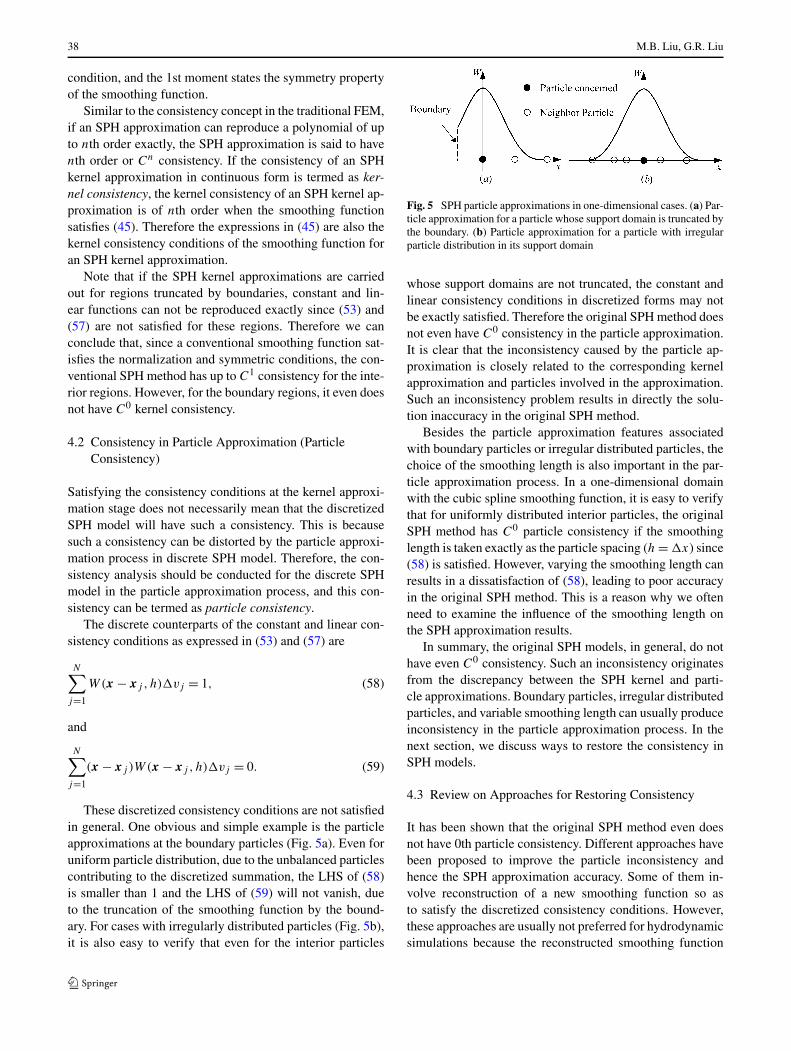
These discretized consistency conditions are not satisfiedin general. One obvious and simple example is the particleapproximations at the boundary particles (Fig. 5a). Even foruniform particle distribution, due to the unbalanced particlescontributing to the discretized summation, the LHS of (58)is smaller than 1 and the LHS of (59) will not vanish, dueto the truncation of the smoothing function by the bound-ary. For cases with irregularly distributed particles (Fig. 5b),it is also easy to verify that even for the interior particles
Fig. 5 SPH particle approximations in one-dimensional cases. (a) Par-ticle approximation for a particle whose support domain is truncated bythe boundary. (b) Particle approximation for a particle with irregularparticle distribution in its support domain
whose support domains are not truncated, the constant andlinear consistency conditions in discretized forms may notbe exactly satisfied. Therefore the original SPH method doesnot even have C0 consistency in the particle approximation.It is clear that the inconsistency caused by the particle ap-proximation is closely related to the corresponding kernelapproximation and particles involved in the approximation.Such an inconsistency problem results in directly the solu-tion inaccuracy in the original SPH method.
Besides the particle approximation features associatedwith boundary particles or irregular distributed particles, thechoice of the smoothing length is also important in the par-ticle approximation process. In a one-dimensional domainwith the cubic spline smoothing function, it is easy to verifythat for uniformly distributed interior particles, the originalSPH method has C0 particle consistency if the smoothinglength is taken exactly as the particle spacing (h = �x) since(58) is satisfied. However, varying the smoothing length canresults in a dissatisfaction of (58), leading to poor accuracyin the original SPH method. This is a reason why we oftenneed to examine the influence of the smoothing length onthe SPH approximation results.
In summary, the original SPH models, in general, do nothave even C0 consistency. Such an inconsistency originatesfrom the discrepancy between the SPH kernel and parti-cle approximations. Boundary particles, irregular distributedparticles, and variable smoothing length can usually produceinconsistency in the particle approximation process. In thenext section, we discuss ways to restore the consistency inSPH models.
4.3 Review on Approaches for Restoring Consistency
It has been shown that the original SPH method even doesnot have 0th particle consistency. Different approaches havebeen proposed to improve the particle inconsistency andhence the SPH approximation accuracy. Some of them in-volve reconstruction of a new smoothing function so asto satisfy the discretized consistency conditions. However,these approaches are usually not preferred for hydrodynamicsimulations because the reconstructed smoothing function
Smoothed Particle Hydrodynamics (SPH): an Overview and Recent Developments 39
can be partially negative, non-symmetric, and not monoton-ically decreasing. Approaches which improve the particleconsistency without changing the conventional smoothingfunction are usually more preferable in simulating hydrody-namics.
One early approach [49, 52] is based on the anti-symmetric assumption of the derivative of a smoothing func-tion
N∑j=1
Wi,α�vj = 0, (60)
where Wi,α = ∂Wi(x)/∂xα , in which α is the dimensionindex repeated from 1 to d (d is the number of dimen-sions). Therefore when approximating the derivative of afunction f , the particle approximation can be rewritten as
fi,α =N∑
j=1
(fj − fi)Wi,α�vj , (61)
or
fi,α =N∑
j=1
(fj + fi)Wi,α�vj . (62)
It should also be noted that (60) is not necessarily valid, evenif its corresponding continuous counterpart
∫Wi,αdx = 0 is
valid (for interior regions). This is also a manifestation ofthe particle inconsistency. Therefore (61) and (62) actuallyuse the particle inconsistency in approximating the deriva-tive of the smoothing function to offset or balance the parti-cle inconsistency in approximating the derivatives of a fieldfunction, with a hope to improve the accuracy of the approx-imations.
Randles and Libersky [52] derived a normalization for-mulation for the density approximation
ρi =∑N
j=1 ρjWij�vj∑Nj=1 Wij�vj
, (63)
and a normalization for the divergence of the stress tensor σ
(∇ · σ)i =∑N
j=1(σj − σi) ⊗ ∇iWij�vj∑Nj=1(xj − xi ) ⊗ ∇iWij�vj
, (64)
where ⊗ is the tensor product. Again, (63) and (64) also usethe inconsistency in approximating the smoothing functionand its derivatives to offset the inconsistency in approximat-ing a field function and its derivatives, also with an aim toimprove the accuracy of the approximations.
Based on Taylor series expansion on the SPH approxi-mation of a function, Chen et al. [54] suggested a correc-tive smoothed particle method (CSPM). In one-dimensionalspace, the process of CSPM can be briefed as follows.
Performing Taylor series expansion at a nearby point xi ,a sufficiently smooth function f (x) can be expressed as
f (x) = fi + (x − xi)fi,x + (x − xi)2
2! fi,xx + · · · . (65)
Multiplying both sides of (65) by the smoothing function W
and integrating over the entire computational domain yield∫
f (x)Wi(x)dx
= fi
∫Wi(x)dx + fi,x
∫(x − xi)Wi(x)dx
+ fi,xx
2
∫(x − xi)
2Wi(x)dx + · · · . (66)
If the terms involving derivatives in this equation are ne-glected, a corrective kernel approximation for function f (x)
at particle i is obtained as
fi =∫
f (x)Wi(x)dx∫Wi(x)dx
. (67)
For a conventional smoothing function (non-negative andsymmetric), the second term at the RHS of (66) is zero forinterior region and not zero for boundary region. Thereforethe corrective kernel approximation expressed in (67) is alsoof 2nd order accuracy for interior region and 1st order ac-curacy for boundary region. Comparing (67) with (16), it isfound that for the interior regions, the kernel approximationsin the original SPH and CSPM are actually the same dueto the satisfaction of the normalization condition (in con-tinuous form). For the boundary regions, since the integralof the smoothing function is truncated by the boundary, thenormalization condition cannot be satisfied. By retaining thenon-unity denominator, CSPM restores the C0 kernel con-sistency.
The corresponding particle approximation for functionf (x) at particle i can be obtained using summation overnearest particles for each term in (66) and again neglectingthe terms related to derivatives
fi =∑N
j=1 fjWij�vj∑Nj=1 Wij�vj
. (68)
It is noted that the particle approximation of the second termat the RHS of (66) is not necessarily zero even for the inte-rior particles due to the irregularity of the particles. There-fore strictly speaking, the particle approximation expressedin (68) is of 1st order accuracy for both the interior andboundary particles. Only if the particles are uniformly dis-tributed can the particle approximation of the second termat the RHS of (66) be zero. In this case, the particle approx-imation expressed in (68) is of 2nd order accuracy for theuniformly distributed interior particles.
40 M.B. Liu, G.R. Liu
If replacing Wi(x) in (66) with Wi,x and neglecting thesecond and higher derivatives, a corrective kernel approxi-mation for the first derivative is generated as
fi,x =∫ [f (x) − f (xi)]Wi,x(x)dx∫
(x − xi)Wi,x(x)dx. (69)
The particle approximations corresponding to (69) is
fi,x =∑N
j=1(fj − fi)Wi,x�vj∑Nj=1(xj − xi )Wi,x�vj
. (70)
Similarly, The CSPM kernel approximations for thederivatives are also of second order accuracy (or 1st or-der consistency) for interior regions, but 1st order accu-racy (or 0th order consistency) for boundary regions. Ex-cept for cases with uniformly distributed interior particles,the CSPM particle approximations for the derivatives are of1st order accuracy (or 0th order consistency) for both theinterior and boundary particles.
4.4 An SPH Formulation for Discontinuity
It is clear that CSPM can have better accuracy than theconventional SPH method as it improves the boundary de-ficiency problem. It was reported that the CSPM can alsoreduce the so-called tensile instability inherent in the tradi-tional SPH method [89, 90].
One notable point in CSPM is that it is based on Tay-lor series analysis on the kernel approximation of a fieldfunction and its derivatives. To perform Taylor series analy-sis, the function under consideration should be sufficientlysmooth. Therefore, CSPM is not applicable to problemswith discontinuities such as hydrodynamic problems thatgenerate shock waves.
Liu and his co-workers proposed a further improvementon SPH in resolving discontinuity problems, and they callthis as a discontinuous SPH, or DSPH [55]. The idea ofDSPH one-dimensional space is briefed here as follows.
Examine the kernel approximation for any function f (x)
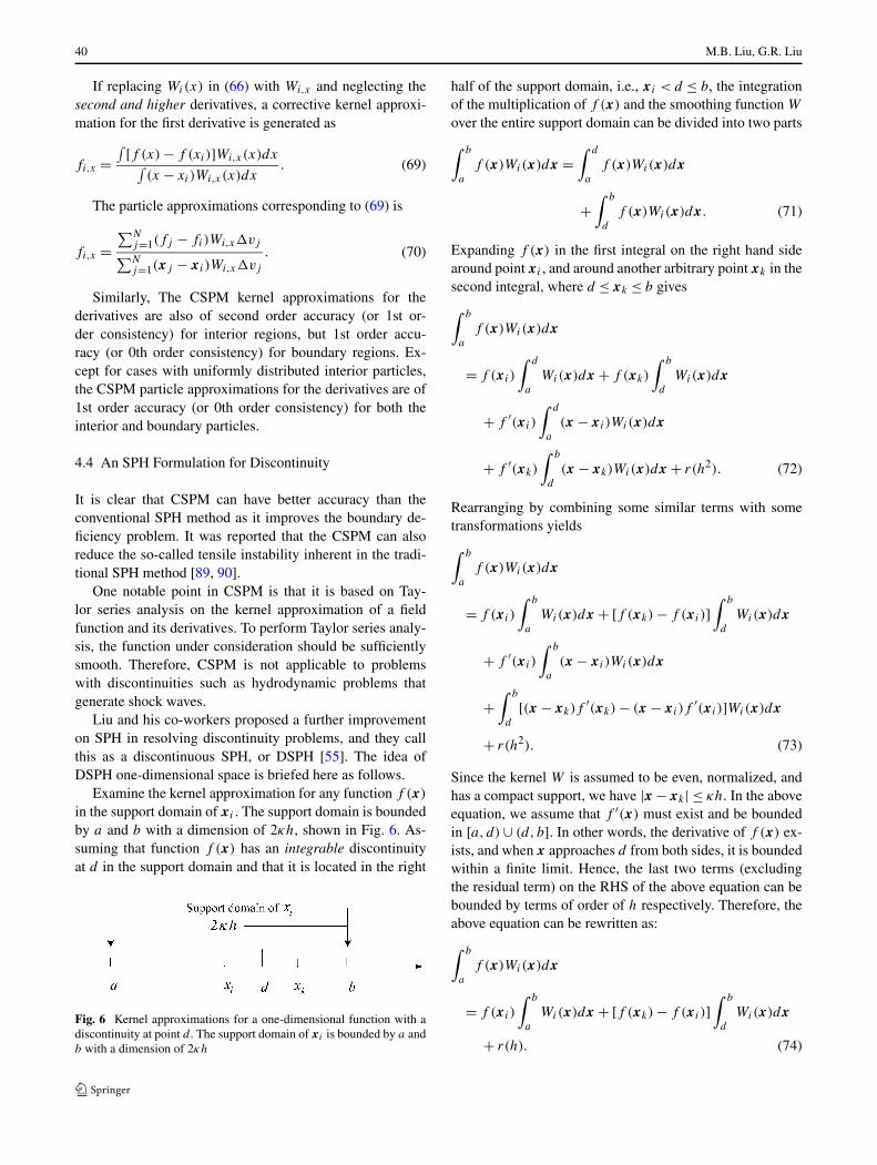
in the support domain of xi . The support domain is boundedby a and b with a dimension of 2κh, shown in Fig. 6. As-suming that function f (x) has an integrable discontinuityat d in the support domain and that it is located in the right
Fig. 6 Kernel approximations for a one-dimensional function with adiscontinuity at point d . The support domain of xi is bounded by a andb with a dimension of 2κh
half of the support domain, i.e., xi < d ≤ b, the integrationof the multiplication of f (x) and the smoothing function W
over the entire support domain can be divided into two parts
∫ b
a
f (x)Wi(x)dx =∫ d
a
f (x)Wi(x)dx
+∫ b
d
f (x)Wi(x)dx. (71)
Expanding f (x) in the first integral on the right hand sidearound point xi , and around another arbitrary point xk in thesecond integral, where d ≤ xk ≤ b gives
∫ b
a
f (x)Wi(x)dx
= f (xi )
∫ d
a
Wi(x)dx + f (xk)
∫ b
d
Wi(x)dx
+ f ′(xi )
∫ d
a
(x − xi )Wi(x)dx
+ f ′(xk)
∫ b
d
(x − xk)Wi(x)dx + r(h2). (72)
Rearranging by combining some similar terms with sometransformations yields
∫ b
a
f (x)Wi(x)dx
= f (xi )
∫ b
a
Wi(x)dx + [f (xk) − f (xi )]∫ b
d
Wi(x)dx
+ f ′(xi )
∫ b
a
(x − xi )Wi(x)dx
+∫ b
d
[(x − xk)f′(xk) − (x − xi )f
′(xi )]Wi(x)dx
+ r(h2). (73)
Since the kernel W is assumed to be even, normalized, andhas a compact support, we have |x − xk| ≤ κh. In the aboveequation, we assume that f ′(x) must exist and be boundedin [a, d) ∪ (d, b]. In other words, the derivative of f (x) ex-ists, and when x approaches d from both sides, it is boundedwithin a finite limit. Hence, the last two terms (excludingthe residual term) on the RHS of the above equation can bebounded by terms of order of h respectively. Therefore, theabove equation can be rewritten as:
∫ b
a
f (x)Wi(x)dx
= f (xi )
∫ b
a
Wi(x)dx + [f (xk) − f (xi )]∫ b
d
Wi(x)dx
+ r(h). (74)
Smoothed Particle Hydrodynamics (SPH): an Overview and Recent Developments 41
This equation can be re-written as
f (xi ) =∫ b
af (x)Wi(x)dx∫ b
aWi(x)dx
−{ [f (xk) − f (xi )]
∫ b
dWi(x)dx∫ b
aWi(x)dx
}+ r(h), (75)
which is the kernel approximation of the field function witha discontinuity.
Similarly, the kernel approximation of the derivative isobtained as
f ′(xi )
=∫ b
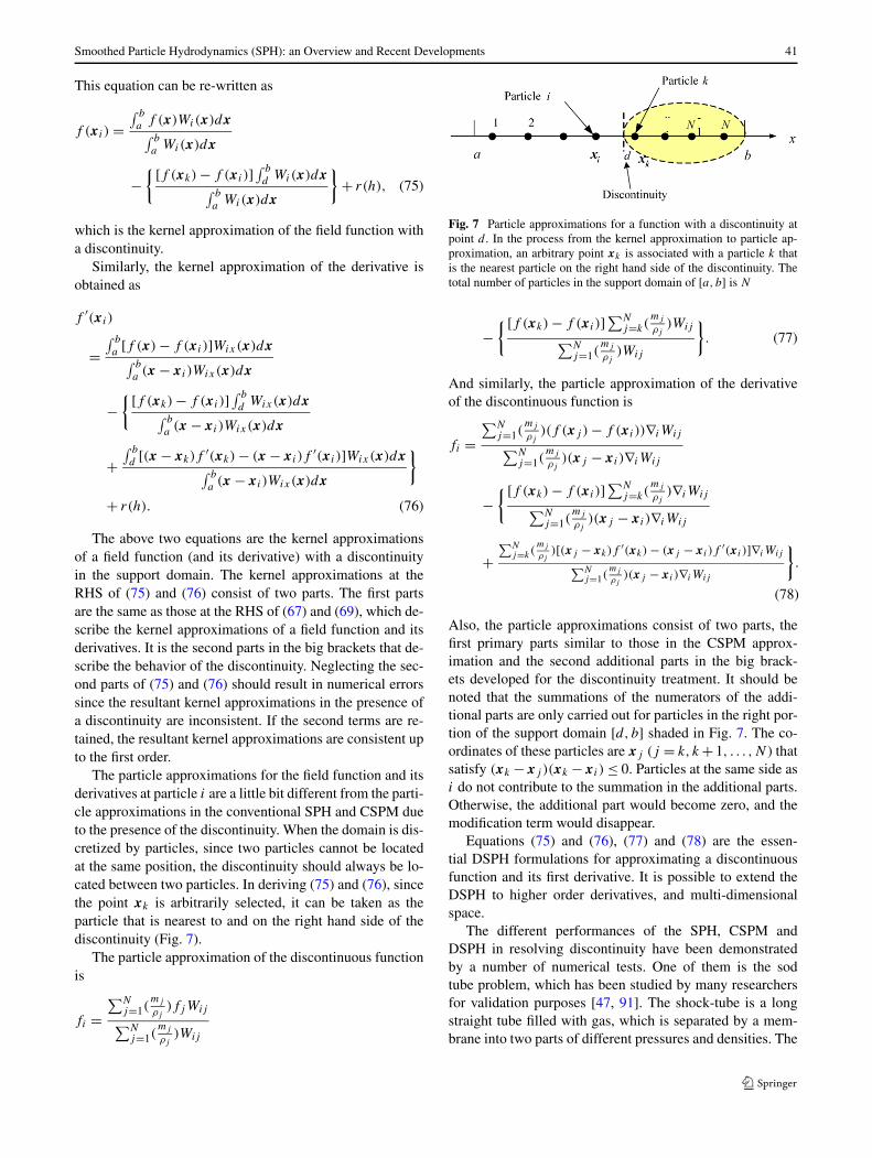
a[f (x) − f (xi )]Wix(x)dx∫ b
a(x − xi )Wix(x)dx
−{ [f (xk) − f (xi )]
∫ b
dWix(x)dx∫ b
a(x − xi )Wix(x)dx
+∫ b
d[(x − xk)f
′(xk) − (x − xi )f′(xi )]Wix(x)dx∫ b
a(x − xi )Wix(x)dx
}
+ r(h). (76)
The above two equations are the kernel approximationsof a field function (and its derivative) with a discontinuityin the support domain. The kernel approximations at theRHS of (75) and (76) consist of two parts. The first partsare the same as those at the RHS of (67) and (69), which de-scribe the kernel approximations of a field function and itsderivatives. It is the second parts in the big brackets that de-scribe the behavior of the discontinuity. Neglecting the sec-ond parts of (75) and (76) should result in numerical errorssince the resultant kernel approximations in the presence ofa discontinuity are inconsistent. If the second terms are re-tained, the resultant kernel approximations are consistent upto the first order.
The particle approximations for the field function and itsderivatives at particle i are a little bit different from the parti-cle approximations in the conventional SPH and CSPM dueto the presence of the discontinuity. When the domain is dis-cretized by particles, since two particles cannot be locatedat the same position, the discontinuity should always be lo-cated between two particles. In deriving (75) and (76), sincethe point xk is arbitrarily selected, it can be taken as theparticle that is nearest to and on the right hand side of thediscontinuity (Fig. 7).
The particle approximation of the discontinuous functionis
fi =∑N
j=1(mj
ρj)fjWij∑N
j=1(mj
ρj)Wij
Fig. 7 Particle approximations for a function with a discontinuity atpoint d . In the process from the kernel approximation to particle ap-proximation, an arbitrary point xk is associated with a particle k thatis the nearest particle on the right hand side of the discontinuity. Thetotal number of particles in the support domain of [a, b] is N
−{ [f (xk) − f (xi )]∑N
j=k(mj
ρj)Wij∑N
j=1(mj
ρj)Wij
}. (77)
And similarly, the particle approximation of the derivativeof the discontinuous function is
fi =∑N
j=1(mj
ρj)(f (xj ) − f (xi ))∇iWij∑N
j=1(mj
ρj)(xj − xi )∇iWij
−{ [f (xk) − f (xi )]∑N
j=k(mj
ρj)∇iWij∑N
j=1(mj
ρj)(xj − xi )∇iWij
+∑N
j=k(mj
ρj)[(xj − xk)f
′(xk) − (xj − xi )f′(xi )]∇iWij∑N
j=1(mj
ρj)(xj − xi )∇iWij
}.
(78)
Also, the particle approximations consist of two parts, thefirst primary parts similar to those in the CSPM approx-imation and the second additional parts in the big brack-ets developed for the discontinuity treatment. It should benoted that the summations of the numerators of the addi-tional parts are only carried out for particles in the right por-tion of the support domain [d, b] shaded in Fig. 7. The co-ordinates of these particles are xj (j = k, k + 1, . . . ,N ) thatsatisfy (xk − xj )(xk − xi ) ≤ 0. Particles at the same side asi do not contribute to the summation in the additional parts.Otherwise, the additional part would become zero, and themodification term would disappear.
Equations (75) and (76), (77) and (78) are the essen-tial DSPH formulations for approximating a discontinuousfunction and its first derivative. It is possible to extend theDSPH to higher order derivatives, and multi-dimensionalspace.
The different performances of the SPH, CSPM andDSPH in resolving discontinuity have been demonstratedby a number of numerical tests. One of them is the sodtube problem, which has been studied by many researchersfor validation purposes [47, 91]. The shock-tube is a longstraight tube filled with gas, which is separated by a mem-brane into two parts of different pressures and densities. The
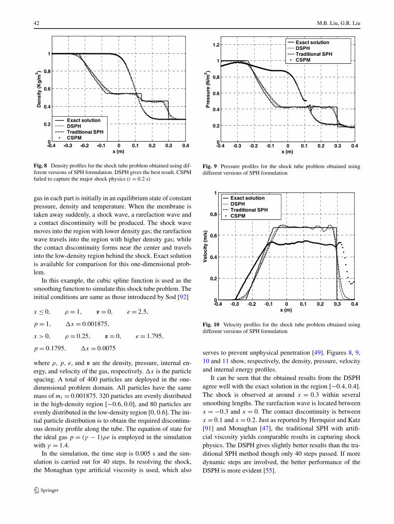
42 M.B. Liu, G.R. Liu
Fig. 8 Density profiles for the shock tube problem obtained using dif-ferent versions of SPH formulation. DSPH gives the best result. CSPMfailed to capture the major shock physics (t = 0.2 s)
gas in each part is initially in an equilibrium state of constantpressure, density and temperature. When the membrane istaken away suddenly, a shock wave, a rarefaction wave anda contact discontinuity will be produced. The shock wavemoves into the region with lower density gas; the rarefactionwave travels into the region with higher density gas; whilethe contact discontinuity forms near the center and travelsinto the low-density region behind the shock. Exact solutionis available for comparison for this one-dimensional prob-lem.
In this example, the cubic spline function is used as thesmoothing function to simulate this shock tube problem. Theinitial conditions are same as those introduced by Sod [92]
x ≤ 0, ρ = 1, v = 0, e = 2.5,
p = 1, �x = 0.001875,
x > 0, ρ = 0.25, v = 0, e = 1.795,
p = 0.1795, �x = 0.0075
where ρ, p, e, and v are the density, pressure, internal en-ergy, and velocity of the gas, respectively. �x is the particlespacing. A total of 400 particles are deployed in the one-dimensional problem domain. All particles have the samemass of mi = 0.001875. 320 particles are evenly distributedin the high-density region [−0.6,0.0], and 80 particles areevenly distributed in the low-density region [0,0.6]. The ini-tial particle distribution is to obtain the required discontinu-ous density profile along the tube. The equation of state forthe ideal gas p = (γ − 1)ρe is employed in the simulationwith γ = 1.4.
In the simulation, the time step is 0.005 s and the sim-ulation is carried out for 40 steps. In resolving the shock,the Monaghan type artificial viscosity is used, which also
Fig. 9 Pressure profiles for the shock tube problem obtained usingdifferent versions of SPH formulation
Fig. 10 Velocity profiles for the shock tube problem obtained usingdifferent versions of SPH formulation
serves to prevent unphysical penetration [49]. Figures 8, 9,10 and 11 show, respectively, the density, pressure, velocityand internal energy profiles.
It can be seen that the obtained results from the DSPHagree well with the exact solution in the region [−0.4,0.4].The shock is observed at around x = 0.3 within severalsmoothing lengths. The rarefaction wave is located betweenx = −0.3 and x = 0. The contact discontinuity is betweenx = 0.1 and x = 0.2. Just as reported by Hernquist and Katz[91] and Monaghan [47], the traditional SPH with artifi-cial viscosity yields comparable results in capturing shockphysics. The DSPH gives slightly better results than the tra-ditional SPH method though only 40 steps passed. If moredynamic steps are involved, the better performance of theDSPH is more evident [55].
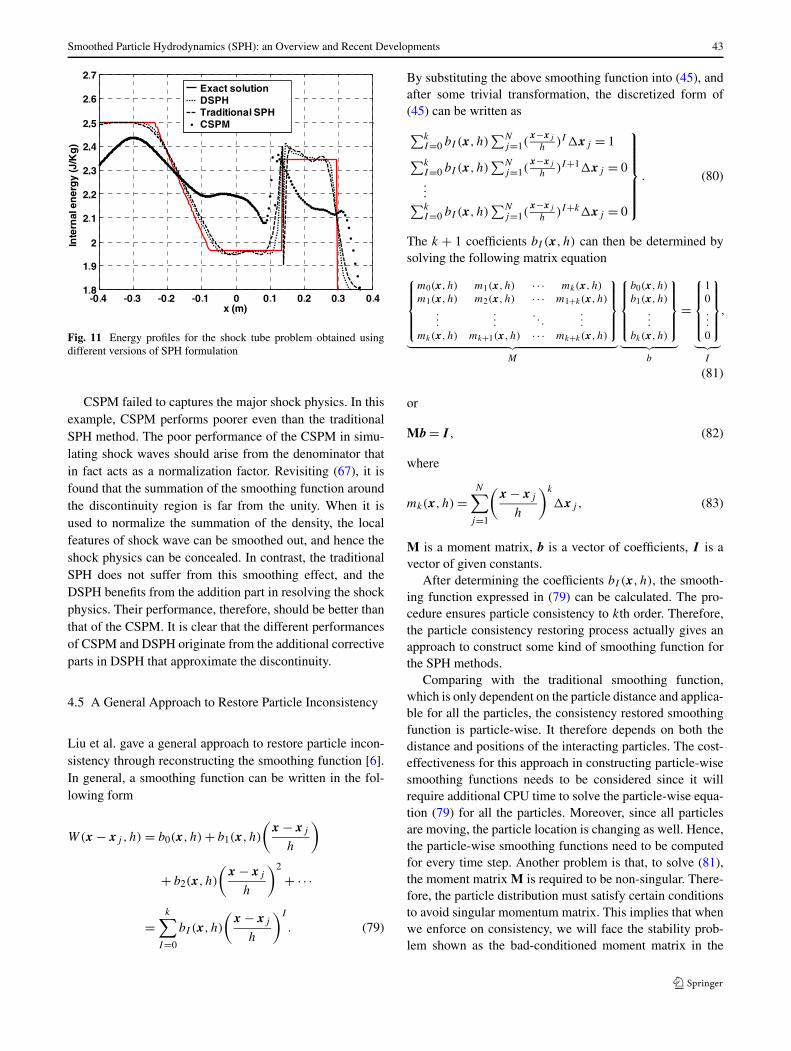
Smoothed Particle Hydrodynamics (SPH): an Overview and Recent Developments 43
Fig. 11 Energy profiles for the shock tube problem obtained usingdifferent versions of SPH formulation
CSPM failed to captures the major shock physics. In thisexample, CSPM performs poorer even than the traditionalSPH method. The poor performance of the CSPM in simu-lating shock waves should arise from the denominator thatin fact acts as a normalization factor. Revisiting (67), it isfound that the summation of the smoothing function aroundthe discontinuity region is far from the unity. When it isused to normalize the summation of the density, the localfeatures of shock wave can be smoothed out, and hence theshock physics can be concealed. In contrast, the traditionalSPH does not suffer from this smoothing effect, and theDSPH benefits from the addition part in resolving the shockphysics. Their performance, therefore, should be better thanthat of the CSPM. It is clear that the different performancesof CSPM and DSPH originate from the additional correctiveparts in DSPH that approximate the discontinuity.
4.5 A General Approach to Restore Particle Inconsistency
Liu et al. gave a general approach to restore particle incon-sistency through reconstructing the smoothing function [6].In general, a smoothing function can be written in the fol-lowing form
W(x − xj , h) = b0(x, h) + b1(x, h)
(x − xj
h
)
+ b2(x, h)
(x − xj
h
)2
+ · · ·
=k∑
I=0
bI (x, h)
(x − xj
h
)I
. (79)
By substituting the above smoothing function into (45), andafter some trivial transformation, the discretized form of(45) can be written as
∑kI=0 bI (x, h)
∑Nj=1(
x−xj
h)I�xj = 1
∑kI=0 bI (x, h)
∑Nj=1(
x−xj
h)I+1�xj = 0
...∑kI=0 bI (x, h)
∑Nj=1(
x−xj
h)I+k�xj = 0
⎫⎪⎪⎪⎪⎪⎬⎪⎪⎪⎪⎪⎭
. (80)
The k + 1 coefficients bI (x, h) can then be determined bysolving the following matrix equation
⎧⎪⎪⎪⎨⎪⎪⎪⎩
m0(x, h) m1(x, h) · · · mk(x, h)
m1(x, h) m2(x, h) · · · m1+k(x, h)
.
.
....
. . ....
mk(x, h) mk+1(x, h) · · · mk+k(x, h)
⎫⎪⎪⎪⎬⎪⎪⎪⎭
︸ ︷︷ ︸M
⎧⎪⎪⎪⎨⎪⎪⎪⎩
b0(x, h)
b1(x, h)
.
.
.
bk(x, h)
⎫⎪⎪⎪⎬⎪⎪⎪⎭
︸ ︷︷ ︸b
=
⎧⎪⎪⎪⎨⎪⎪⎪⎩
10...
0
⎫⎪⎪⎪⎬⎪⎪⎪⎭
︸ ︷︷ ︸I
,
(81)
or
Mb = I , (82)
where
mk(x, h) =N∑
j=1
(x − xj
h
)k
�xj , (83)
M is a moment matrix, b is a vector of coefficients, I is avector of given constants.
After determining the coefficients bI (x, h), the smooth-ing function expressed in (79) can be calculated. The pro-cedure ensures particle consistency to kth order. Therefore,the particle consistency restoring process actually gives anapproach to construct some kind of smoothing function forthe SPH methods.
Comparing with the traditional smoothing function,which is only dependent on the particle distance and applica-ble for all the particles, the consistency restored smoothingfunction is particle-wise. It therefore depends on both thedistance and positions of the interacting particles. The cost-effectiveness for this approach in constructing particle-wisesmoothing functions needs to be considered since it willrequire additional CPU time to solve the particle-wise equa-tion (79) for all the particles. Moreover, since all particlesare moving, the particle location is changing as well. Hence,the particle-wise smoothing functions need to be computedfor every time step. Another problem is that, to solve (81),the moment matrix M is required to be non-singular. There-fore, the particle distribution must satisfy certain conditionsto avoid singular momentum matrix. This implies that whenwe enforce on consistency, we will face the stability prob-lem shown as the bad-conditioned moment matrix in the
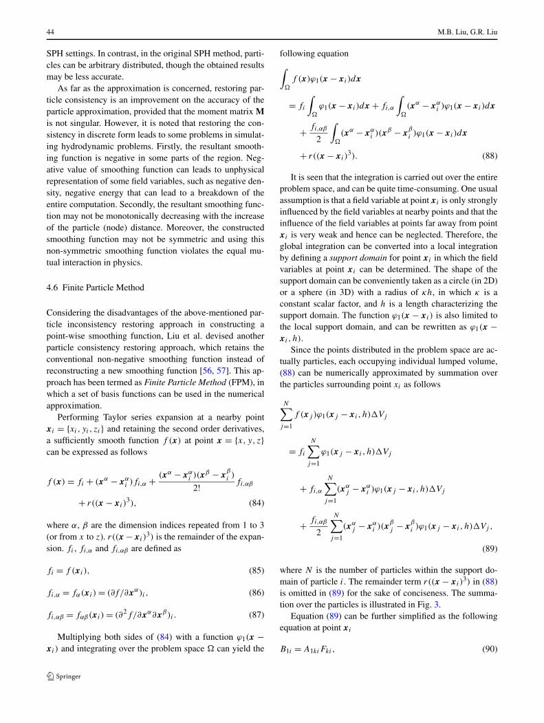
44 M.B. Liu, G.R. Liu
SPH settings. In contrast, in the original SPH method, parti-cles can be arbitrary distributed, though the obtained resultsmay be less accurate.
As far as the approximation is concerned, restoring par-ticle consistency is an improvement on the accuracy of theparticle approximation, provided that the moment matrix Mis not singular. However, it is noted that restoring the con-sistency in discrete form leads to some problems in simulat-ing hydrodynamic problems. Firstly, the resultant smooth-ing function is negative in some parts of the region. Neg-ative value of smoothing function can leads to unphysicalrepresentation of some field variables, such as negative den-sity, negative energy that can lead to a breakdown of theentire computation. Secondly, the resultant smoothing func-tion may not be monotonically decreasing with the increaseof the particle (node) distance. Moreover, the constructedsmoothing function may not be symmetric and using thisnon-symmetric smoothing function violates the equal mu-tual interaction in physics.
4.6 Finite Particle Method
Considering the disadvantages of the above-mentioned par-ticle inconsistency restoring approach in constructing apoint-wise smoothing function, Liu et al. devised anotherparticle consistency restoring approach, which retains theconventional non-negative smoothing function instead ofreconstructing a new smoothing function [56, 57]. This ap-proach has been termed as Finite Particle Method (FPM), inwhich a set of basis functions can be used in the numericalapproximation.
Performing Taylor series expansion at a nearby pointxi = {xi, yi, zi} and retaining the second order derivatives,a sufficiently smooth function f (x) at point x = {x, y, z}can be expressed as follows
f (x) = fi + (xα − xαi )fi,α + (xα − xα
i )(xβ − xβi )
2! fi,αβ
+ r((x − xi )3), (84)
where α, β are the dimension indices repeated from 1 to 3(or from x to z). r((x − xi )
3) is the remainder of the expan-sion. fi , fi,α and fi,αβ are defined as
fi = f (xi ), (85)
fi,α = fα(xi ) = (∂f/∂xα)i, (86)
fi,αβ = fαβ(xi ) = (∂2f/∂xα∂xβ)i . (87)
Multiplying both sides of (84) with a function ϕ1(x −xi ) and integrating over the problem space � can yield the
following equation
∫�
f (x)ϕ1(x − xi )dx
= fi
∫�
ϕ1(x − xi )dx + fi,α
∫�
(xα − xαi )ϕ1(x − xi )dx
+ fi,αβ
2
∫�
(xα − xαi )(xβ − x
βi )ϕ1(x − xi )dx
+ r((x − xi )3). (88)
It is seen that the integration is carried out over the entireproblem space, and can be quite time-consuming. One usualassumption is that a field variable at point xi is only stronglyinfluenced by the field variables at nearby points and that theinfluence of the field variables at points far away from pointxi is very weak and hence can be neglected. Therefore, theglobal integration can be converted into a local integrationby defining a support domain for point xi in which the fieldvariables at point xi can be determined. The shape of thesupport domain can be conveniently taken as a circle (in 2D)or a sphere (in 3D) with a radius of κh, in which κ is aconstant scalar factor, and h is a length characterizing thesupport domain. The function ϕ1(x − xi ) is also limited tothe local support domain, and can be rewritten as ϕ1(x −xi , h).
Since the points distributed in the problem space are ac-tually particles, each occupying individual lumped volume,(88) can be numerically approximated by summation overthe particles surrounding point xi as follows
N∑j=1
f (xj )ϕ1(xj − xi , h)�Vj
= fi
N∑j=1
ϕ1(xj − xi , h)�Vj
+ fi,α
N∑j=1
(xαj − xα
i )ϕ1(xj − xi , h)�Vj
+ fi,αβ
2
N∑j=1
(xαj − xα
i )(xβj − x
βi )ϕ1(xj − xi , h)�Vj ,
(89)
where N is the number of particles within the support do-main of particle i. The remainder term r((x − xi )
3) in (88)is omitted in (89) for the sake of conciseness. The summa-tion over the particles is illustrated in Fig. 3.
Equation (89) can be further simplified as the followingequation at point xi
B1i = A1kiFki, (90)
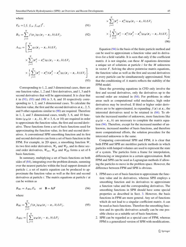
Smoothed Particle Hydrodynamics (SPH): an Overview and Recent Developments 45
where
Fki = [fi fi,α fi,αβ ]T , (91)
B1i =N∑
j=1
f (xj )ϕ1(xj − xi , h)�Vj , (92)
A1ki =[
N∑j=1
ϕ1(xj − xi , h)�Vj
×N∑
j=1
(xαj − xα
i )ϕ1(xj − xi , h)�Vj
× 1
2
N∑j=1
(xαj − xα
i )(xβj − x
βi )ϕ1(xj − xi , h)�Vj
].
(93)
Corresponding to 1, 2, and 3 dimensional cases, there areone function value, 1, 2 and 3 first derivatives, and 1, 3 and 6second derivatives that will be approximated. It is clear thatk in (91), (93) and (90) is 3, 6, and 10 respectively corre-sponding to 1, 2, and 3 dimensional cases. To calculate thefunction value, the first and the second derivatives at xi , 2, 5,and 9 other equations similar to (90) are required. Thereforein 1, 2, and 3 dimensional cases, totally 3, 6, and 10 func-tions (ϕM(x − xi , h), M = 3, 6, or 10) are required in orderto approximate the function value, the first and second deriv-ative. These functions form a set of basis functions used forapproximating the function value, its first and second deriv-atives. A conventional SPH smoothing function and its firstand second derivatives can form a set of basis function in theFPM. For example, in 2D space, a smoothing function W ,its two first order derivatives, Wα and Wβ , and its three sec-ond order derivatives, Wαα , Wαβ and Wββ forms a set of 6basis functions.
In summary, multiplying a set of basis functions on bothsides of (84), integrating over the problem domain, summingover the nearest particles within the local support domain ofparticle i, a set of matrix equation can be produced to ap-proximate the function value as well as the first and secondderivatives at particle i. The matrix equations at particle i atcan be written as
BMi = AMkiFki or B = AF (94)
where
BMi =N∑
j=1
f (xj )ϕM(xj − xi , h)�Vj , (95)
AMki =[
N∑j=1
ϕM(xj − xi , h)�Vj
×N∑
j=1
(xαj − xα
i )ϕM(xj − xi , h)�Vj
× 1
2
N∑j=1
(xαj − xα
i )(xβj − x
βi )ϕM(xj − xi , h)�Vj
].
(96)
Equation (94) is the basis of the finite particle method andcan be used to approximate a function value and its deriva-tives for a field variable. It is seen that only if the coefficientmatrix A is not singular, can these M equations determinea unique set of solutions at particle i for the M unknownsin vector F . Solving the above pointwise matrix equations,the function value as well as the first and second derivativesat every particle can be simultaneously approximated. Notethat the conditioning of A matrix reflects the stability of theFPM model.
Since the governing equations in CFD only involve thefirst and second derivatives, only the derivatives up to thesecond order are retained in (84). For problems in otherareas such as computational solid mechanics, high orderderivatives may be involved. If third or higher order deriv-atives are to be approximated, in expanding f (x) at xi , theinterested derivatives need to be retained in (84). To ob-tain the increased number of unknowns, more functions likeϕM(x − xi , h) are necessary to complete the matrix equa-tion (94). Therefore, except for the increased number of un-knowns, increased number of basis functions, and thereforemore computational efforts, the solution procedure for theinterested unknowns is the same.
Comparing conventional SPH and FPM, it is clear thatboth FPM and SPH are meshfree particle methods in whichparticles with lumped volumes are used to represent the stateof a system. The particles form a frame for interpolation,differencing or integration in a certain approximation. BothFPM and SPH can be used as Lagrangian methods if allow-ing the particles to move in the problem space. However, thedifference between FPM and SPH is obvious.
1. FPM uses a set of basis function to approximate the func-tion value and its derivatives, whereas SPH employs asmoothing function and its derivatives to approximatea function value and the corresponding derivatives. Thesmoothing functions in SPH should have some specialproperties as described in Sect. 3. However, the basisfunctions in FPM are more general. Any set of functionswhich do not lead to a singular coefficient matrix A canbe used as basis functions. Therefore the smoothing func-tion and its specific derivatives actually can be one pos-sible choice as a suitable set of basis functions.
2. SPH can be regarded as a special case of FPM, whereasFPM is a generalized version of SPH with modifications.
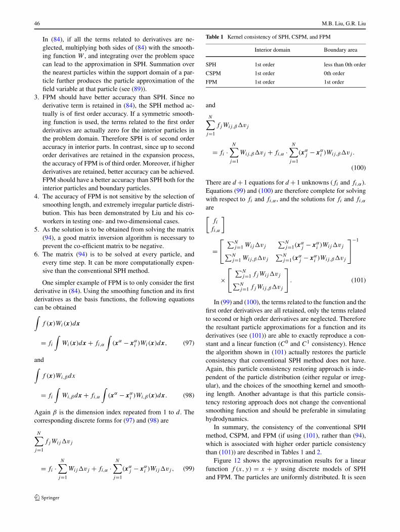
46 M.B. Liu, G.R. Liu
In (84), if all the terms related to derivatives are ne-glected, multiplying both sides of (84) with the smooth-ing function W , and integrating over the problem spacecan lead to the approximation in SPH. Summation overthe nearest particles within the support domain of a par-ticle further produces the particle approximation of thefield variable at that particle (see (89)).
3. FPM should have better accuracy than SPH. Since noderivative term is retained in (84), the SPH method ac-tually is of first order accuracy. If a symmetric smooth-ing function is used, the terms related to the first orderderivatives are actually zero for the interior particles inthe problem domain. Therefore SPH is of second orderaccuracy in interior parts. In contrast, since up to secondorder derivatives are retained in the expansion process,the accuracy of FPM is of third order. Moreover, if higherderivatives are retained, better accuracy can be achieved.FPM should have a better accuracy than SPH both for theinterior particles and boundary particles.
4. The accuracy of FPM is not sensitive by the selection ofsmoothing length, and extremely irregular particle distri-bution. This has been demonstrated by Liu and his co-workers in testing one- and two-dimensional cases.
5. As the solution is to be obtained from solving the matrix(94), a good matrix inversion algorithm is necessary toprevent the co-efficient matrix to be negative.
6. The matrix (94) is to be solved at every particle, andevery time step. It can be more computationally expen-sive than the conventional SPH method.
One simpler example of FPM is to only consider the firstderivative in (84). Using the smoothing function and its firstderivatives as the basis functions, the following equationscan be obtained∫
f (x)Wi(x)dx
= fi
∫Wi(x)dx + fi,α
∫(xα − xα
i )Wi(x)dx, (97)
and∫f (x)Wi,βdx
= fi
∫Wi,βdx + fi,α
∫(xα − xα
i )Wi,β(x)dx. (98)
Again β is the dimension index repeated from 1 to d . Thecorresponding discrete forms for (97) and (98) are
N∑j=1
fjWij�vj
= fi ·N∑
j=1
Wij�vj + fi,α ·N∑
j=1
(xαj − xα
i )Wij�vj , (99)
Table 1 Kernel consistency of SPH, CSPM, and FPM
Interior domain Boundary area
SPH 1st order less than 0th order
CSPM 1st order 0th order
FPM 1st order 1st order
and
N∑j=1
fjWij,β�vj
= fi ·N∑
j=1
Wij,β�vj + fi,α ·N∑
j=1
(xαj − xα
i )Wij,β�vj .
(100)
There are d + 1 equations for d + 1 unknowns (fi and fi,α).Equations (99) and (100) are therefore complete for solvingwith respect to fi and fi,α , and the solutions for fi and fi,α
are[
fi
fi,α
]
=⎡⎣
∑Nj=1 Wij�vj
∑Nj=1(x
αj − xα
i )Wij�vj∑Nj=1 Wij,β�vj
∑Nj=1(x
αj − xα
i )Wij,β�vj
⎤⎦
−1
×⎡⎣
∑Nj=1 fjWij�vj∑N
j=1 fjWij,β�vj
⎤⎦ . (101)
In (99) and (100), the terms related to the function and thefirst order derivatives are all retained, only the terms relatedto second or high order derivatives are neglected. Thereforethe resultant particle approximations for a function and itsderivatives (see (101)) are able to exactly reproduce a con-stant and a linear function (C0 and C1 consistency). Hencethe algorithm shown in (101) actually restores the particleconsistency that conventional SPH method does not have.Again, this particle consistency restoring approach is inde-pendent of the particle distribution (either regular or irreg-ular), and the choices of the smoothing kernel and smooth-ing length. Another advantage is that this particle consis-tency restoring approach does not change the conventionalsmoothing function and should be preferable in simulatinghydrodynamics.
In summary, the consistency of the conventional SPHmethod, CSPM, and FPM (if using (101), rather than (94),which is associated with higher order particle consistencythan (101)) are described in Tables 1 and 2.
Figure 12 shows the approximation results for a linearfunction f (x, y) = x + y using discrete models of SPHand FPM. The particles are uniformly distributed. It is seen
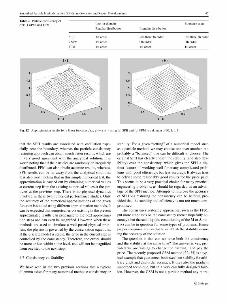
Smoothed Particle Hydrodynamics (SPH): an Overview and Recent Developments 47
Table 2 Particle consistency ofSPH, CSPM, and FPM Interior domain Boundary area
Regular distribution Irregular distribution
SPH 1st order less than 0th order less than 0th order
CSPM 1st order 0th order 0th order
FPM 1st order 1st order 1st order
Fig. 12 Approximation results for a linear function f (x, y) = x + y using (a) SPH and (b) FPM in a domain of [0,1,0,1]
that the SPH results are associated with oscillation espe-cially near the boundary, whereas the particle consistencyrestoring approach can obtain much better results, which arein very good agreement with the analytical solution. It isworth noting that if the particles are randomly or irregularlydistributed, FPM can also obtain accurate results, whereas,SPH results can be far away from the analytical solutions.It is also worth noting that in this simple numerical test, theapproximation is carried out by obtaining numerical valuesat current step from the existing numerical values at the par-ticles at the previous step. There is no physical dynamicsinvolved in these two numerical performance studies. Onlythe accuracy of the numerical approximations of the givenfunction is studied using different approximation methods. Itcan be expected that numerical errors existing in the presentapproximated results can propagate to the next approxima-tion steps and can even be magnified. However, when thesemethods are used to simulate a well-posed physical prob-lem, the physics is governed by the conservation equations.If the discrete model is stable, the error in the current step iscontrolled by the consistency. Therefore, the errors shouldbe more or less within some level, and will not be magnifiedfrom one step to the next step.
4.7 Consistency vs. Stability
We have seen in the two previous sections that a typicaldilemma exists for many numerical methods: consistency or
stability. For a given “setting” of a numerical model suchas a particle method, we may choose one over another, butprobably a “balanced” one can be difficult to choose. Theoriginal SPH has clearly chosen the stability (and also flex-ibility) over the consistency, which gives the SPH a dis-tinct feature of working well for many complicated prob-lems with good efficiency, but less accuracy. It always triesto deliver some reasonably good results for the price paid.This seems to be a very practical choice for many practicalengineering problems, as should be regarded as an advan-tage of the SPH method. Attempts to improve the accuracyof SPH via restoring the consistency can be helpful, pro-vided that the stability and efficiency is not too much com-promised.
The consistency restoring approaches, such as the FPM,put more emphases on the consistency (hence hopefully ac-curacy), but the stability (the conditioning of the M or A ma-trix) can be in question for some types of problems. Henceproper measures are needed to establish the stability ensur-ing the accuracy of the solution.
The question is that can we have both the consistencyand the stability at the same time? The answer is yes, pro-vided we are willing to change the “setting” and pay theprice. The recently proposed GSM method [32–35] is a typ-ical example that guarantees both excellent stability for arbi-trary grids and 2nd order accuracy. It uses also the gradientsmoothed technique, but in a very carefully designed fash-ion. However, the GSM is not a particle method any more;
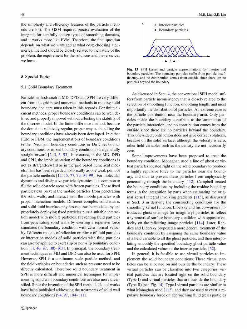
48 M.B. Liu, G.R. Liu
the simplicity and efficiency features of the particle meth-ods are lost. The GSM requires precise evaluation of theintegrals for carefully chosen types of smoothing domains,and it works more like FVM. Therefore, the final questiondepends on what we want and at what cost: choosing a nu-merical method should be closely related to the nature of theproblem, the requirement for the solutions and the resourceswe have.
5 Special Topics
5.1 Solid Boundary Treatment
Particle methods such as MD, DPD, and SPH are very differ-ent from the grid based numerical methods in treating solidboundary, and care must taken in this regards. For finite el-ement methods, proper boundary conditions can be well de-fined and properly imposed without affecting the stability ofthe discrete model. In the finite difference method, becausethe domain is relatively regular, proper ways to handling theboundary conditions have already been developed. In eitherFEM or FDM, the implementations of boundary conditions(either Neumann boundary conditions or Dirichlet bound-ary conditions, or mixed boundary conditions) are generallystraightforward [2, 3, 5, 93]. In contrast, in the MD, DPDand SPH, the implementation of the boundary conditions isnot as straightforward as in the grid based numerical mod-els. This has been regarded historically as one weak point ofthe particle methods [12, 15, 77, 79, 94–99]. For moleculardynamics and dissipative particle dynamics, it is common tofill the solid obstacle areas with frozen particles. These fixedparticles can prevent the mobile particles from penetratingthe solid walls, and interact with the mobile particles withproper interaction models. Different complex solid matrixand solid-fluid interface physics can thus be modeled by ap-propriately deploying fixed particles plus a suitable interac-tion model with mobile particles. Preventing fluid particlesfrom penetrating solid walls by exerting a repulsive forcesimulates the boundary condition with zero normal veloc-ity. Different models of reflection or mirror of fluid particlesor interaction models of solid particles with fluid particlescan also be applied to exert slip or non-slip boundary condi-tion [11, 40, 97, 100–103]. In principal, the boundary treat-ment techniques in MD and DPD can also be used for SPH.However, SPH is a continuum scale particle method, andthe field variables on boundaries such as pressure need to bedirectly calculated. Therefore solid boundary treatment inSPH is more difficult and numerical techniques for imple-menting solid wall boundary conditions are also more diver-sified. Since the invention of the SPH method, a lot of workshave been published addressing the treatments of solid wallboundary conditions [94, 97, 104–111].
Fig. 13 SPH kernel and particle approximations for interior andboundary particles. The boundary particles suffer from particle insuf-ficiency, and no contribution comes from outside since there are noparticles beyond the boundary
As discussed in Sect. 4, the conventional SPH model suf-fers from particle inconsistency that is closely related to theselection of smoothing function, smoothing length, and mostimportantly the distribution of particles. An extreme case isthe particle distribution near the boundary area. Only par-ticles inside the boundary contribute to the summation ofthe particle interaction, and no contribution comes from theoutside since there are no particles beyond the boundary.This one-sided contribution does not give correct solutions,because on the solid surface, although the velocity is zero,other field variables such as the density are not necessarilyzero.
Some improvements have been proposed to treat theboundary condition. Monaghan used a line of ghost or vir-tual particles located right on the solid boundary to producea highly repulsive force to the particles near the bound-ary, and thus to prevent these particles from unphysicallypenetrating through the boundary [112]. Campbell treatedthe boundary conditions by including the residue boundaryterms in the integration by parts when estimating the orig-inal kernel integral involving gradients [113], as discussedin Sect. 3 in deriving the constructing conditions for thesmoothing kernel function. Libersky and his co-workers in-troduced ghost or image (or imaginary) particles to reflecta symmetrical surface boundary condition with opposite ve-locity on the reflecting image particles [114]. Later, Ran-dles and Libersky proposed a more general treatment of theboundary condition by assigning the same boundary valueof a field variable to all the ghost particles, and then interpo-lating smoothly the specified boundary ghost particle valueand the calculated values of the interior particles [52].
In general, it is feasible to use virtual particles to im-plement the solid boundary conditions. These virtual par-ticles can be allocated on and outside the boundary. Thesevirtual particles can be classified into two categories, vir-tual particles that are located right on the solid boundary(Type I) and virtual particles that are outside the boundary(Type II) (see Fig. 14). Type I virtual particles are similar towhat Monaghan used [112], and they are used to exert a re-pulsive boundary force on approaching fluid (real) particles
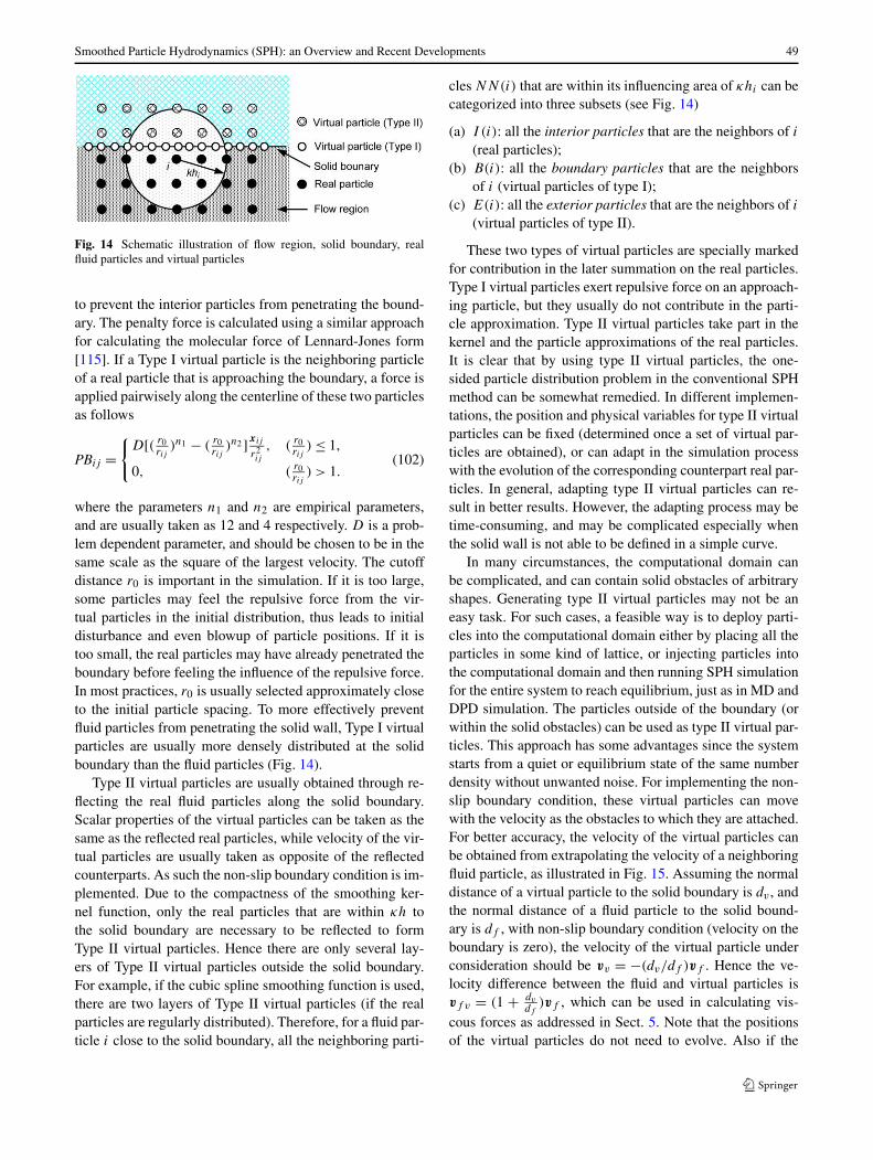
Smoothed Particle Hydrodynamics (SPH): an Overview and Recent Developments 49
Fig. 14 Schematic illustration of flow region, solid boundary, realfluid particles and virtual particles
to prevent the interior particles from penetrating the bound-ary. The penalty force is calculated using a similar approachfor calculating the molecular force of Lennard-Jones form[115]. If a Type I virtual particle is the neighboring particleof a real particle that is approaching the boundary, a force isapplied pairwisely along the centerline of these two particlesas follows
PBij ={
D[( r0rij
)n1 − (r0rij
)n2 ]xij
r2ij
, (r0rij
) ≤ 1,
0, (r0rij
) > 1.(102)
where the parameters n1 and n2 are empirical parameters,and are usually taken as 12 and 4 respectively. D is a prob-lem dependent parameter, and should be chosen to be in thesame scale as the square of the largest velocity. The cutoffdistance r0 is important in the simulation. If it is too large,some particles may feel the repulsive force from the vir-tual particles in the initial distribution, thus leads to initialdisturbance and even blowup of particle positions. If it istoo small, the real particles may have already penetrated theboundary before feeling the influence of the repulsive force.In most practices, r0 is usually selected approximately closeto the initial particle spacing. To more effectively preventfluid particles from penetrating the solid wall, Type I virtualparticles are usually more densely distributed at the solidboundary than the fluid particles (Fig. 14).
Type II virtual particles are usually obtained through re-flecting the real fluid particles along the solid boundary.Scalar properties of the virtual particles can be taken as thesame as the reflected real particles, while velocity of the vir-tual particles are usually taken as opposite of the reflectedcounterparts. As such the non-slip boundary condition is im-plemented. Due to the compactness of the smoothing ker-nel function, only the real particles that are within κh tothe solid boundary are necessary to be reflected to formType II virtual particles. Hence there are only several lay-ers of Type II virtual particles outside the solid boundary.For example, if the cubic spline smoothing function is used,there are two layers of Type II virtual particles (if the realparticles are regularly distributed). Therefore, for a fluid par-ticle i close to the solid boundary, all the neighboring parti-
cles NN(i) that are within its influencing area of κhi can becategorized into three subsets (see Fig. 14)
(a) I (i): all the interior particles that are the neighbors of i
(real particles);(b) B(i): all the boundary particles that are the neighbors
of i (virtual particles of type I);(c) E(i): all the exterior particles that are the neighbors of i
(virtual particles of type II).
These two types of virtual particles are specially markedfor contribution in the later summation on the real particles.Type I virtual particles exert repulsive force on an approach-ing particle, but they usually do not contribute in the parti-cle approximation. Type II virtual particles take part in thekernel and the particle approximations of the real particles.It is clear that by using type II virtual particles, the one-sided particle distribution problem in the conventional SPHmethod can be somewhat remedied. In different implemen-tations, the position and physical variables for type II virtualparticles can be fixed (determined once a set of virtual par-ticles are obtained), or can adapt in the simulation processwith the evolution of the corresponding counterpart real par-ticles. In general, adapting type II virtual particles can re-sult in better results. However, the adapting process may betime-consuming, and may be complicated especially whenthe solid wall is not able to be defined in a simple curve.
In many circumstances, the computational domain canbe complicated, and can contain solid obstacles of arbitraryshapes. Generating type II virtual particles may not be aneasy task. For such cases, a feasible way is to deploy parti-cles into the computational domain either by placing all theparticles in some kind of lattice, or injecting particles intothe computational domain and then running SPH simulationfor the entire system to reach equilibrium, just as in MD andDPD simulation. The particles outside of the boundary (orwithin the solid obstacles) can be used as type II virtual par-ticles. This approach has some advantages since the systemstarts from a quiet or equilibrium state of the same numberdensity without unwanted noise. For implementing the non-slip boundary condition, these virtual particles can movewith the velocity as the obstacles to which they are attached.For better accuracy, the velocity of the virtual particles canbe obtained from extrapolating the velocity of a neighboringfluid particle, as illustrated in Fig. 15. Assuming the normaldistance of a virtual particle to the solid boundary is dv , andthe normal distance of a fluid particle to the solid bound-ary is df , with non-slip boundary condition (velocity on theboundary is zero), the velocity of the virtual particle underconsideration should be vv = −(dv/df )vf . Hence the ve-locity difference between the fluid and virtual particles isvf v = (1 + dv
df)vf , which can be used in calculating vis-
cous forces as addressed in Sect. 5. Note that the positionsof the virtual particles do not need to evolve. Also if the
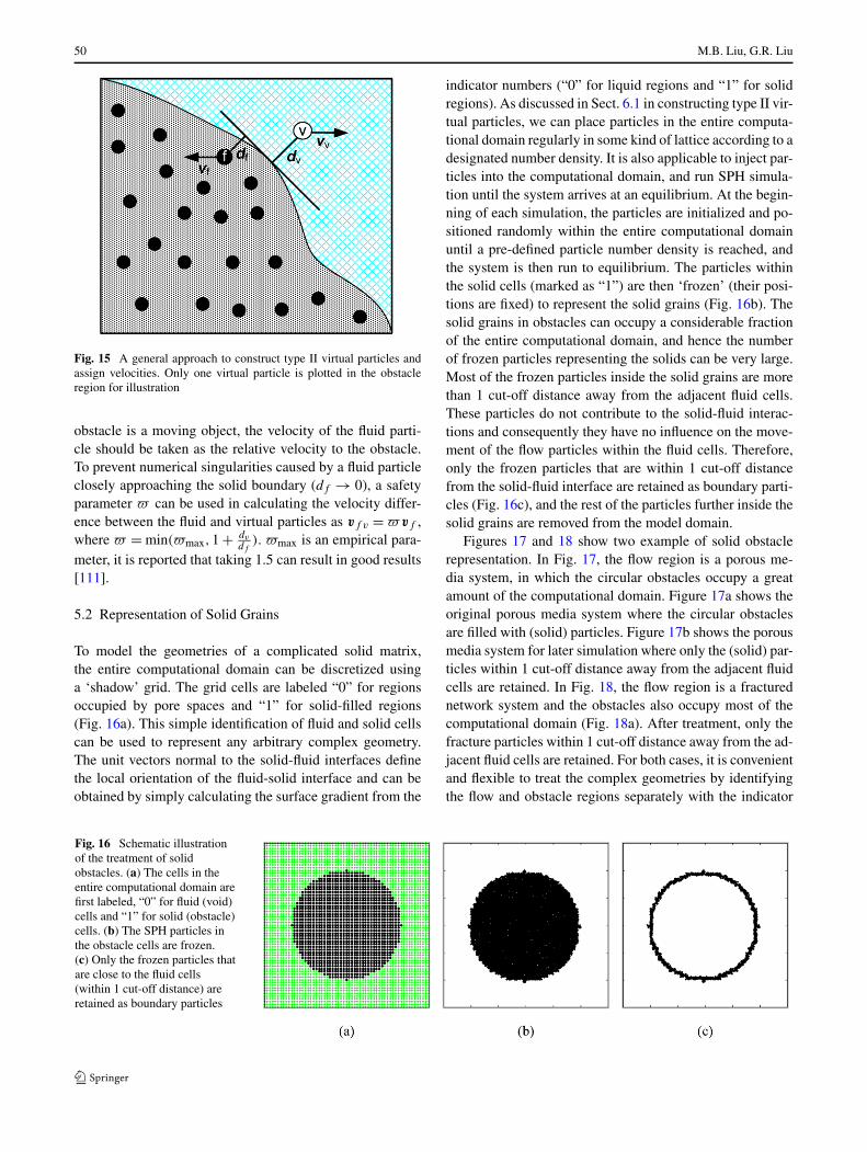
50 M.B. Liu, G.R. Liu
Fig. 15 A general approach to construct type II virtual particles andassign velocities. Only one virtual particle is plotted in the obstacleregion for illustration
obstacle is a moving object, the velocity of the fluid parti-cle should be taken as the relative velocity to the obstacle.To prevent numerical singularities caused by a fluid particleclosely approaching the solid boundary (df → 0), a safetyparameter � can be used in calculating the velocity differ-ence between the fluid and virtual particles as vf v = �vf ,where � = min(�max,1 + dv
df). �max is an empirical para-
meter, it is reported that taking 1.5 can result in good results[111].
5.2 Representation of Solid Grains
To model the geometries of a complicated solid matrix,the entire computational domain can be discretized usinga ‘shadow’ grid. The grid cells are labeled “0” for regionsoccupied by pore spaces and “1” for solid-filled regions(Fig. 16a). This simple identification of fluid and solid cellscan be used to represent any arbitrary complex geometry.The unit vectors normal to the solid-fluid interfaces definethe local orientation of the fluid-solid interface and can beobtained by simply calculating the surface gradient from the
indicator numbers (“0” for liquid regions and “1” for solidregions). As discussed in Sect. 6.1 in constructing type II vir-tual particles, we can place particles in the entire computa-tional domain regularly in some kind of lattice according to adesignated number density. It is also applicable to inject par-ticles into the computational domain, and run SPH simula-tion until the system arrives at an equilibrium. At the begin-ning of each simulation, the particles are initialized and po-sitioned randomly within the entire computational domainuntil a pre-defined particle number density is reached, andthe system is then run to equilibrium. The particles withinthe solid cells (marked as “1”) are then ‘frozen’ (their posi-tions are fixed) to represent the solid grains (Fig. 16b). Thesolid grains in obstacles can occupy a considerable fractionof the entire computational domain, and hence the numberof frozen particles representing the solids can be very large.Most of the frozen particles inside the solid grains are morethan 1 cut-off distance away from the adjacent fluid cells.These particles do not contribute to the solid-fluid interac-tions and consequently they have no influence on the move-ment of the flow particles within the fluid cells. Therefore,only the frozen particles that are within 1 cut-off distancefrom the solid-fluid interface are retained as boundary parti-cles (Fig. 16c), and the rest of the particles further inside thesolid grains are removed from the model domain.
Figures 17 and 18 show two example of solid obstaclerepresentation. In Fig. 17, the flow region is a porous me-dia system, in which the circular obstacles occupy a greatamount of the computational domain. Figure 17a shows theoriginal porous media system where the circular obstaclesare filled with (solid) particles. Figure 17b shows the porousmedia system for later simulation where only the (solid) par-ticles within 1 cut-off distance away from the adjacent fluidcells are retained. In Fig. 18, the flow region is a fracturednetwork system and the obstacles also occupy most of thecomputational domain (Fig. 18a). After treatment, only thefracture particles within 1 cut-off distance away from the ad-jacent fluid cells are retained. For both cases, it is convenientand flexible to treat the complex geometries by identifyingthe flow and obstacle regions separately with the indicator
Fig. 16 Schematic illustrationof the treatment of solidobstacles. (a) The cells in theentire computational domain arefirst labeled, “0” for fluid (void)cells and “1” for solid (obstacle)cells. (b) The SPH particles inthe obstacle cells are frozen.(c) Only the frozen particles thatare close to the fluid cells(within 1 cut-off distance) areretained as boundary particles
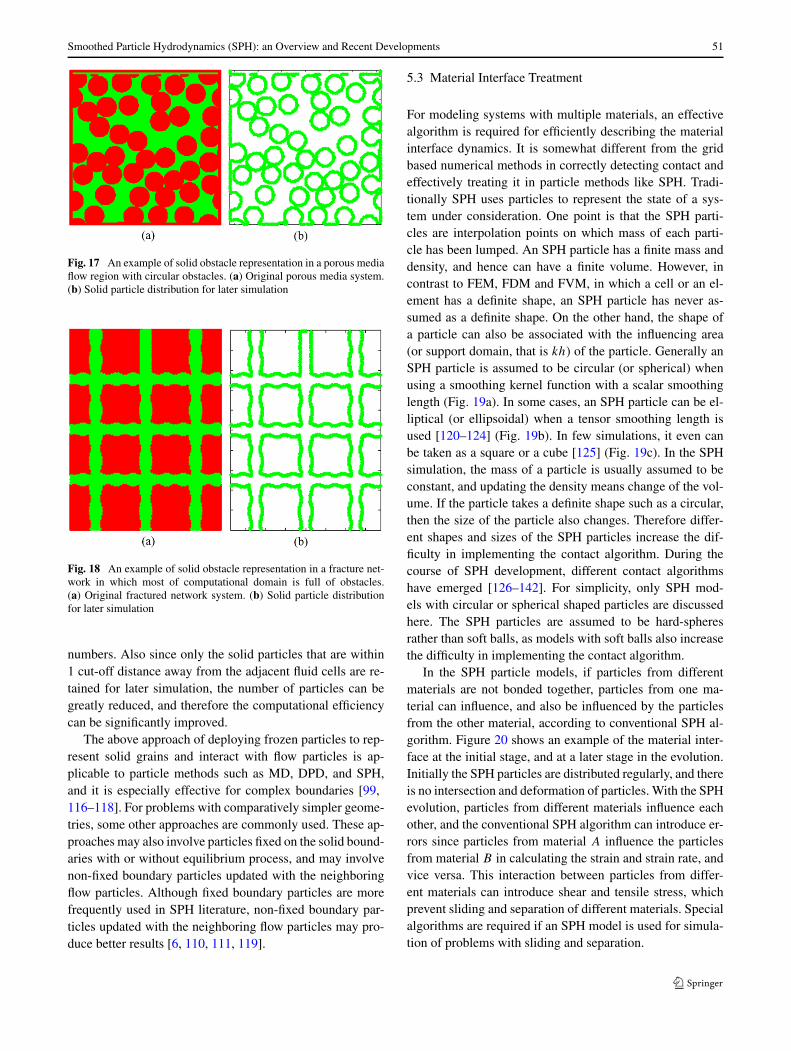
Smoothed Particle Hydrodynamics (SPH): an Overview and Recent Developments 51
Fig. 17 An example of solid obstacle representation in a porous mediaflow region with circular obstacles. (a) Original porous media system.(b) Solid particle distribution for later simulation
Fig. 18 An example of solid obstacle representation in a fracture net-work in which most of computational domain is full of obstacles.(a) Original fractured network system. (b) Solid particle distributionfor later simulation
numbers. Also since only the solid particles that are within1 cut-off distance away from the adjacent fluid cells are re-tained for later simulation, the number of particles can begreatly reduced, and therefore the computational efficiencycan be significantly improved.
The above approach of deploying frozen particles to rep-resent solid grains and interact with flow particles is ap-plicable to particle methods such as MD, DPD, and SPH,and it is especially effective for complex boundaries [99,116–118]. For problems with comparatively simpler geome-tries, some other approaches are commonly used. These ap-proaches may also involve particles fixed on the solid bound-aries with or without equilibrium process, and may involvenon-fixed boundary particles updated with the neighboringflow particles. Although fixed boundary particles are morefrequently used in SPH literature, non-fixed boundary par-ticles updated with the neighboring flow particles may pro-duce better results [6, 110, 111, 119].
5.3 Material Interface Treatment
For modeling systems with multiple materials, an effectivealgorithm is required for efficiently describing the materialinterface dynamics. It is somewhat different from the gridbased numerical methods in correctly detecting contact andeffectively treating it in particle methods like SPH. Tradi-tionally SPH uses particles to represent the state of a sys-tem under consideration. One point is that the SPH parti-cles are interpolation points on which mass of each parti-cle has been lumped. An SPH particle has a finite mass anddensity, and hence can have a finite volume. However, incontrast to FEM, FDM and FVM, in which a cell or an el-ement has a definite shape, an SPH particle has never as-sumed as a definite shape. On the other hand, the shape ofa particle can also be associated with the influencing area(or support domain, that is kh) of the particle. Generally anSPH particle is assumed to be circular (or spherical) whenusing a smoothing kernel function with a scalar smoothinglength (Fig. 19a). In some cases, an SPH particle can be el-liptical (or ellipsoidal) when a tensor smoothing length isused [120–124] (Fig. 19b). In few simulations, it even canbe taken as a square or a cube [125] (Fig. 19c). In the SPHsimulation, the mass of a particle is usually assumed to beconstant, and updating the density means change of the vol-ume. If the particle takes a definite shape such as a circular,then the size of the particle also changes. Therefore differ-ent shapes and sizes of the SPH particles increase the dif-ficulty in implementing the contact algorithm. During thecourse of SPH development, different contact algorithmshave emerged [126–142]. For simplicity, only SPH mod-els with circular or spherical shaped particles are discussedhere. The SPH particles are assumed to be hard-spheresrather than soft balls, as models with soft balls also increasethe difficulty in implementing the contact algorithm.
In the SPH particle models, if particles from differentmaterials are not bonded together, particles from one ma-terial can influence, and also be influenced by the particlesfrom the other material, according to conventional SPH al-gorithm. Figure 20 shows an example of the material inter-face at the initial stage, and at a later stage in the evolution.Initially the SPH particles are distributed regularly, and thereis no intersection and deformation of particles. With the SPHevolution, particles from different materials influence eachother, and the conventional SPH algorithm can introduce er-rors since particles from material A influence the particlesfrom material B in calculating the strain and strain rate, andvice versa. This interaction between particles from differ-ent materials can introduce shear and tensile stress, whichprevent sliding and separation of different materials. Specialalgorithms are required if an SPH model is used for simula-tion of problems with sliding and separation.
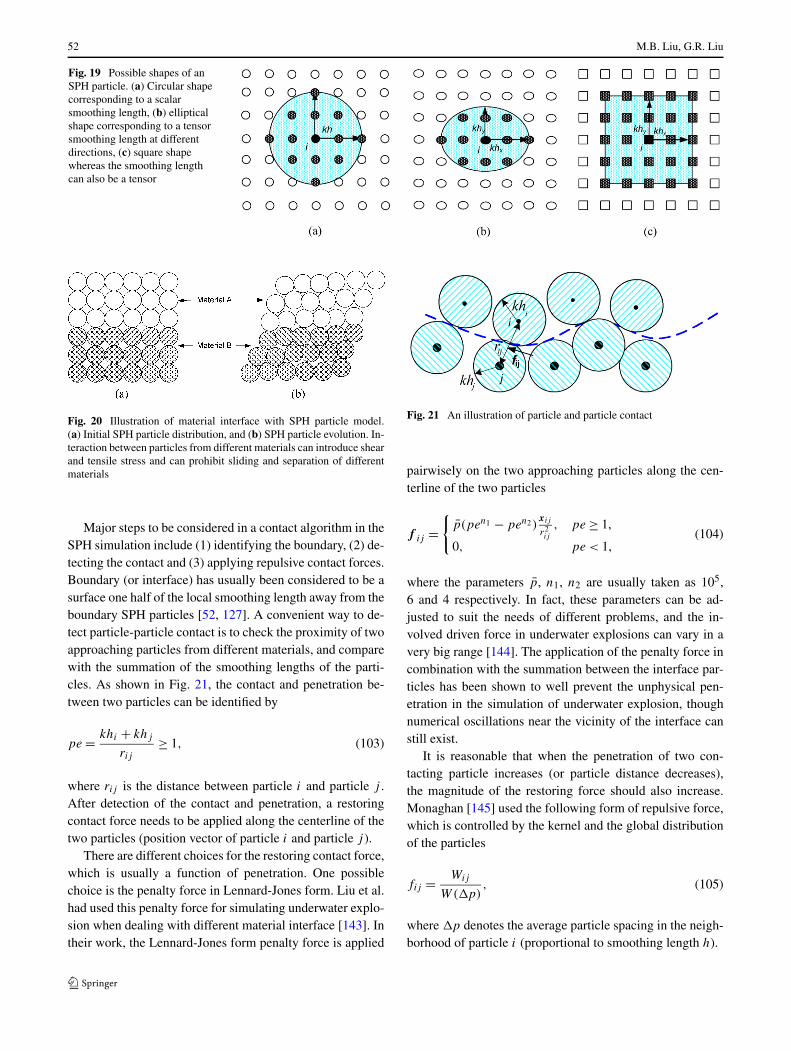
52 M.B. Liu, G.R. Liu
Fig. 19 Possible shapes of anSPH particle. (a) Circular shapecorresponding to a scalarsmoothing length, (b) ellipticalshape corresponding to a tensorsmoothing length at differentdirections, (c) square shapewhereas the smoothing lengthcan also be a tensor
Fig. 20 Illustration of material interface with SPH particle model.(a) Initial SPH particle distribution, and (b) SPH particle evolution. In-teraction between particles from different materials can introduce shearand tensile stress and can prohibit sliding and separation of differentmaterials
Major steps to be considered in a contact algorithm in theSPH simulation include (1) identifying the boundary, (2) de-tecting the contact and (3) applying repulsive contact forces.Boundary (or interface) has usually been considered to be asurface one half of the local smoothing length away from theboundary SPH particles [52, 127]. A convenient way to de-tect particle-particle contact is to check the proximity of twoapproaching particles from different materials, and comparewith the summation of the smoothing lengths of the parti-cles. As shown in Fig. 21, the contact and penetration be-tween two particles can be identified by
pe = khi + khj
rij≥ 1, (103)
where rij is the distance between particle i and particle j .After detection of the contact and penetration, a restoringcontact force needs to be applied along the centerline of thetwo particles (position vector of particle i and particle j ).
There are different choices for the restoring contact force,which is usually a function of penetration. One possiblechoice is the penalty force in Lennard-Jones form. Liu et al.had used this penalty force for simulating underwater explo-sion when dealing with different material interface [143]. Intheir work, the Lennard-Jones form penalty force is applied
Fig. 21 An illustration of particle and particle contact
pairwisely on the two approaching particles along the cen-terline of the two particles
f ij ={
p(pen1 − pen2)xij
r2ij
, pe ≥ 1,
0, pe < 1,(104)
where the parameters p, n1, n2 are usually taken as 105,6 and 4 respectively. In fact, these parameters can be ad-justed to suit the needs of different problems, and the in-volved driven force in underwater explosions can vary in avery big range [144]. The application of the penalty force incombination with the summation between the interface par-ticles has been shown to well prevent the unphysical pen-etration in the simulation of underwater explosion, thoughnumerical oscillations near the vicinity of the interface canstill exist.
It is reasonable that when the penetration of two con-tacting particle increases (or particle distance decreases),the magnitude of the restoring force should also increase.Monaghan [145] used the following form of repulsive force,which is controlled by the kernel and the global distributionof the particles
fij = Wij
W(�p), (105)
where �p denotes the average particle spacing in the neigh-borhood of particle i (proportional to smoothing length h).
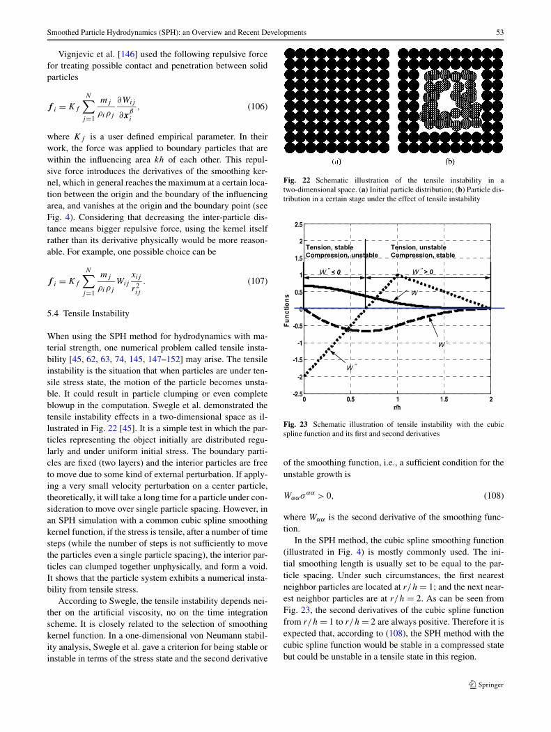
Smoothed Particle Hydrodynamics (SPH): an Overview and Recent Developments 53
Vignjevic et al. [146] used the following repulsive forcefor treating possible contact and penetration between solidparticles
f i = Kf
N∑j=1
mj
ρiρj
∂Wij
∂xβi
, (106)
where Kf is a user defined empirical parameter. In theirwork, the force was applied to boundary particles that arewithin the influencing area kh of each other. This repul-sive force introduces the derivatives of the smoothing ker-nel, which in general reaches the maximum at a certain loca-tion between the origin and the boundary of the influencingarea, and vanishes at the origin and the boundary point (seeFig. 4). Considering that decreasing the inter-particle dis-tance means bigger repulsive force, using the kernel itselfrather than its derivative physically would be more reason-able. For example, one possible choice can be
f i = Kf
N∑j=1
mj
ρiρj
Wij
xij
r2ij
. (107)
5.4 Tensile Instability
When using the SPH method for hydrodynamics with ma-terial strength, one numerical problem called tensile insta-bility [45, 62, 63, 74, 145, 147–152] may arise. The tensileinstability is the situation that when particles are under ten-sile stress state, the motion of the particle becomes unsta-ble. It could result in particle clumping or even completeblowup in the computation. Swegle et al. demonstrated thetensile instability effects in a two-dimensional space as il-lustrated in Fig. 22 [45]. It is a simple test in which the par-ticles representing the object initially are distributed regu-larly and under uniform initial stress. The boundary parti-cles are fixed (two layers) and the interior particles are freeto move due to some kind of external perturbation. If apply-ing a very small velocity perturbation on a center particle,theoretically, it will take a long time for a particle under con-sideration to move over single particle spacing. However, inan SPH simulation with a common cubic spline smoothingkernel function, if the stress is tensile, after a number of timesteps (while the number of steps is not sufficiently to movethe particles even a single particle spacing), the interior par-ticles can clumped together unphysically, and form a void.It shows that the particle system exhibits a numerical insta-bility from tensile stress.
According to Swegle, the tensile instability depends nei-ther on the artificial viscosity, no on the time integrationscheme. It is closely related to the selection of smoothingkernel function. In a one-dimensional von Neumann stabil-ity analysis, Swegle et al. gave a criterion for being stable orinstable in terms of the stress state and the second derivative
Fig. 22 Schematic illustration of the tensile instability in atwo-dimensional space. (a) Initial particle distribution; (b) Particle dis-tribution in a certain stage under the effect of tensile instability
Fig. 23 Schematic illustration of tensile instability with the cubicspline function and its first and second derivatives
of the smoothing function, i.e., a sufficient condition for theunstable growth is
Wαασαα > 0, (108)
where Wαα is the second derivative of the smoothing func-tion.
In the SPH method, the cubic spline smoothing function(illustrated in Fig. 4) is mostly commonly used. The ini-tial smoothing length is usually set to be equal to the par-ticle spacing. Under such circumstances, the first nearestneighbor particles are located at r/h = 1; and the next near-est neighbor particles are at r/h = 2. As can be seen fromFig. 23, the second derivatives of the cubic spline functionfrom r/h = 1 to r/h = 2 are always positive. Therefore it isexpected that, according to (108), the SPH method with thecubic spline function would be stable in a compressed statebut could be unstable in a tensile state in this region.
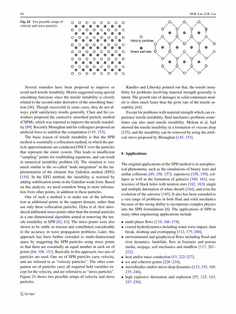
54 M.B. Liu, G.R. Liu
Fig. 24 Two possible setups ofvelocity and stress particles
Several remedies have been proposed to improve oravoid such tensile instability. Morris suggested using specialsmoothing functions since the tensile instability is closelyrelated to the second order derivative of the smoothing func-tion [46]. Though successful in some cases, they do not al-ways yield satisfactory results generally. Chen and his co-workers proposed the corrective smoothed particle method(CSPM), which was reported to improve the tensile instabil-ity [89]. Recently Monaghan and his colleagues proposed anartificial force to stabilize the computation [145, 153].
The basic reason of tensile instability is that the SPHmethod is essentially a collocation method, in which the par-ticle approximations are conducted ONLY over the particlesthat represent the entire system. This leads to insufficient“sampling” points for establishing equations, and can resultin numerical instability problem [4]. The situation is verymuch similar to the so-called “node integration” in the im-plementation of the element free Galerkin method (EFG)[154]. In the EFG method, the instability is restored byadding stabilization terms in the Galerkin weak form. Basedon this analysis, we need somehow bring in more informa-tion from other points, in addition to these particles.
One of such a method is to make use of the informa-tion at additional points in the support domain, rather thanuse only these collocation particles. Dyka et al. first intro-duced additional stress points other than the normal particlesin a one-dimensional algorithm aimed at removing the ten-sile instability in SPH [62, 63]. The stress points were alsoshown to be stable in tension and contributed considerablyto the accuracy in wave propagation problems. Later, thisapproach has been further extended to multi-dimensionalspace by staggering the SPH particles using stress pointsso that there are essentially an equal number in each set ofpoints [64, 108, 151]. Basically in this approach, two sets ofparticles are used. One set of SPH particles carry velocity,and are referred to as “velocity particles”. The other com-panion set of particles carry all required field variables ex-cept for the velocity, and are referred to as “stress particles”.Figure 24 shows two possible setups of velocity and stressparticles.
Randles and Libersky pointed out that, the tensile insta-bility for problems involving material strength generally islatent. The growth rate of damages in solid continuum mod-els is often much faster than the grow rate of the tensile in-stability [64].
Except for problems with material strength which can ex-perience tensile instability, fluid mechanics problems some-times can also meet tensile instability. Melean et al. hadshowed the tensile instability in a formation of viscous drop[155], and the instability can be removed by using the artifi-cial stress proposed by Monaghan [145, 153].
6 Applications
The original applications of the SPH method is in astrophys-ical phenomena, such as the simulations of binary stars andstellar collisions [49, 156, 157], supernova [158, 159], col-lapse as well as the formation of galaxies [160, 161], coa-lescence of black holes with neutron stars [162, 163], singleand multiple detonation of white dwarfs [164], and even theevolution of the universe [165]. It also has been extended toa vast range of problems in both fluid and solid mechanicsbecause of the strong ability to incorporate complex physicsinto the SPH formulations [6]. The applications of SPH tomany other engineering applications include
• multi-phase flows [119, 166–174],• coastal hydrodynamics including water wave impact, dam
break, sloshing and overtopping [112, 175–200],• environmental and geophysical flows including flood and
river dynamics, landslide, flow in fractures and porousmedia, seepage, soil mechanics and mudflow [117, 201–221],
• heat and/or mass conduction [53, 222–227],• ice and cohesive grains [228–234],• microfluidics and/or micro drop dynamics [123, 152, 169,
235–246],• high explosive detonation and explosion [55, 125, 143,
247–256],
Smoothed Particle Hydrodynamics (SPH): an Overview and Recent Developments 55
• underwater explosions and water mitigation [125, 143,247–249, 255],
• elastic and/or plastic flow [52, 114, 257–259],• fracture of brittle solids [260],• metal forming and high pressure die casting [68, 261–
270],• magneto-hydrodynamics and magnetic field simulation
[271–282],• problems with fluid-solid interactions [176, 196, 210,
283–288], and• many other problems like blood flow [289–292], traffic
flow [293].
In this review, we will discuss applications of SPH to thefollowing areas:
• high strain hydrodynamics with material strength,• high explosive detonation and explosions, and underwater
explosion,• microfluidics and micro drop dynamics,• coast hydrodynamics and offshore engineering, and• environmental and geophysical flows.
6.1 High Strain Hydrodynamics with Material Strength
High strain hydrodynamics is generally characterized bythe presence of shock waves, intense localized materialsresponse and impulsive loadings. Numerical simulation ofhigh strain hydrodynamics with material strength such ashigh velocity impact (HVI) and penetrations is one of theformidable but attractive tasks in computational solid me-chanics. Most of the wave propagation hydro-codes use tra-ditional grid based methods such as finite difference meth-ods and finite element methods to simulate high strain hy-drodynamics. Some of them are associated with advancedfeatures which attempt to combine the best advantagesof FDM and FEM. Examples include arbitrary Lagrange-Eulerian (ALE) coupling and coupling Eulerian-Lagrangian(CEL). Though many successful achievements have beenmade using these methods, some numerical difficulties stillexist. These numerical difficulties generally arise from largedeformations, large inhomogeneities, and moving inter-faces, free or movable boundaries [256, 294–297].
SPH method has been intensively used for simulatingsuch phenomena of high strain hydrodynamics with mate-rial strength, due to its special features of meshfree, La-grangian and particle nature. Many researchers have inves-tigated impact (either high velocity or not) and penetrationusing SPH method [50, 51, 86, 129, 132, 134, 139, 140,298–335]. The applications are mainly in defense industry,and typical numerical examples range from Taylor bar im-pacting on a solid wall and spherical projectile/bumper col-lision/penetration [114, 330], projectile impact and penetra-tion and an aircraft fuselage nose impacting a rigid target
[300], to bird strike impacting on an aircraft Wing [335],and even to a high-quality high-fidelity visualization of theSeptember 11 attack on the world trade center [328].
Libersky and his co-workers have carried out the pioneer-ing work of applying the SPH method to high strain hydro-dynamic problems including hyper velocity impact (HVI),fracture and fragmentation [52, 114, 258]. The group fromthe Applied Physics Division of Los Alamos National Lab-oratory (LANL) has modeled high velocity impacts rangingfrom the very small size (femtogram-scale projectiles thathave been accelerated by a Van de Graaf machine to cre-ate craters in various types of targets) to the very large size(Shoemaker-Levy comet impact with the planet Jupiter).Johnson et al. [51, 314] proposed a normalized smooth-ing function (NSF) for axisymmetric problems based on thecondition of uniform strain rate, and have made outstand-ing contributions in the application of SPH to impact prob-lems. Attaway, Pampliton and Swegle et al. have worked incoupling the SPH processor with a transient-dynamics FEMcode, PRONTO, in which high-strain areas that typicallytangle or break conventional finite element meshes are re-solved using the SPH method [126, 336].
Zhou and Liu have revisited the Taylor-Bar-Impact withthe focus on the variation of results corresponding to thedifferent model parameters which represent varied SPHimplementation in a series of three-dimensional computa-tional simulations, and have provided informative data onappropriate SPH implementation options [259]. They alsohave investigated normal and oblique hypervelocity impactsof a sphere on the thin plate, producing large deforma-tion of structures. Figure 25 shows the snapshots of three-dimensional simulation of normal hypervelocity impact ofa sphere on the thin plate at t = 0, 10, 15, and 20 µs. Fig-ure 26 shows the top view (a) and three dimensional view(b) of oblique hypervelocity impact of a sphere on the thinplate at t = 20 µs with a striking angle of 30o. They observedthat for oblique hypervelocity impacts of a sphere on the thinplate, the shape of the crater is no longer in circle, and theshape of the debris cloud changes with different striking an-gles while the ratio of the debris cloud (length over width)remains approximately 1.3.
The standard SPH method uses an isotropic smooth-ing kernel which is characterized by a scalar smoothinglength. One of the problems associated with the standardSPH is that the isotropic kernel of SPH can be seriouslymismatched to the anisotropic volume change that generallyoccur in many problems. To closely match the anisotropicvolume changes, an anisotropic smoothing kernel which canbe characterized by a matrix (in two-dimensional space) ortensor (in three-dimensional space) smoothing length can beefficacious. This leads to the development of the adaptivesmoothed particle hydrodynamics (adaptive SPH or ASPH)in which the smoothing length can be adapted with the vol-ume changes or other dimension-dependent features. The
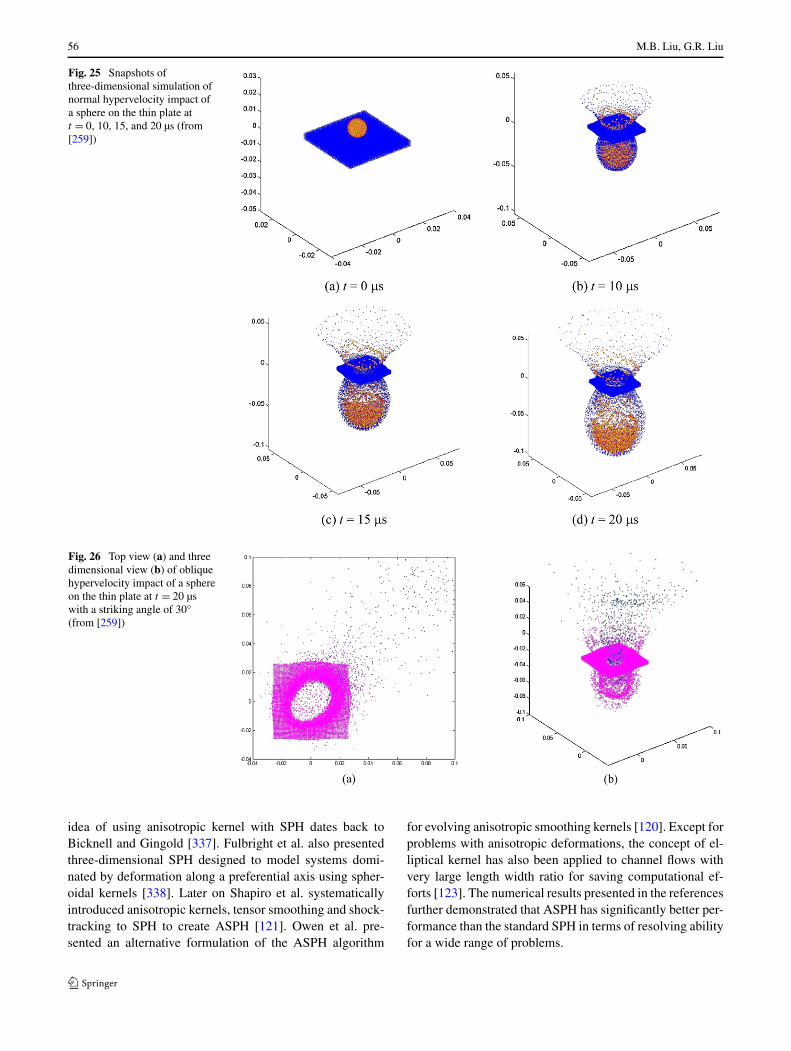
56 M.B. Liu, G.R. Liu
Fig. 25 Snapshots ofthree-dimensional simulation ofnormal hypervelocity impact ofa sphere on the thin plate att = 0, 10, 15, and 20 µs (from[259])
Fig. 26 Top view (a) and threedimensional view (b) of obliquehypervelocity impact of a sphereon the thin plate at t = 20 µswith a striking angle of 30°(from [259])
idea of using anisotropic kernel with SPH dates back toBicknell and Gingold [337]. Fulbright et al. also presentedthree-dimensional SPH designed to model systems domi-nated by deformation along a preferential axis using spher-oidal kernels [338]. Later on Shapiro et al. systematicallyintroduced anisotropic kernels, tensor smoothing and shock-tracking to SPH to create ASPH [121]. Owen et al. pre-sented an alternative formulation of the ASPH algorithm
for evolving anisotropic smoothing kernels [120]. Except forproblems with anisotropic deformations, the concept of el-liptical kernel has also been applied to channel flows withvery large length width ratio for saving computational ef-forts [123]. The numerical results presented in the referencesfurther demonstrated that ASPH has significantly better per-formance than the standard SPH in terms of resolving abilityfor a wide range of problems.
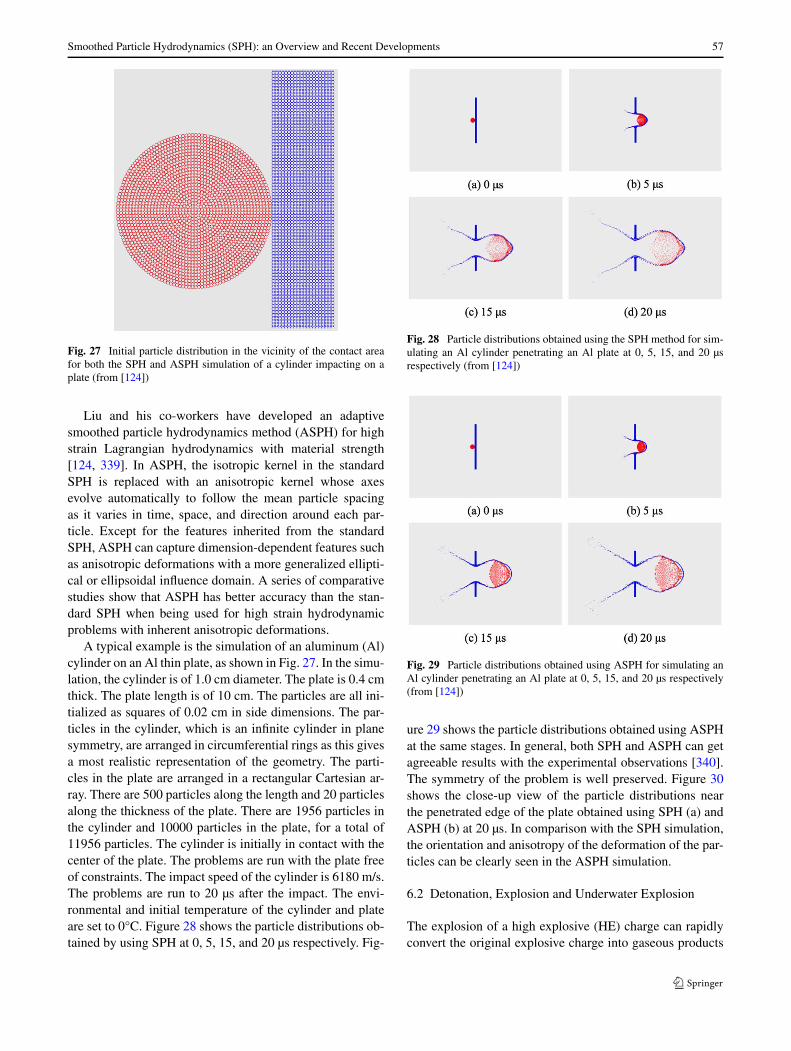
Smoothed Particle Hydrodynamics (SPH): an Overview and Recent Developments 57
Fig. 27 Initial particle distribution in the vicinity of the contact areafor both the SPH and ASPH simulation of a cylinder impacting on aplate (from [124])
Liu and his co-workers have developed an adaptivesmoothed particle hydrodynamics method (ASPH) for highstrain Lagrangian hydrodynamics with material strength[124, 339]. In ASPH, the isotropic kernel in the standardSPH is replaced with an anisotropic kernel whose axesevolve automatically to follow the mean particle spacingas it varies in time, space, and direction around each par-ticle. Except for the features inherited from the standardSPH, ASPH can capture dimension-dependent features suchas anisotropic deformations with a more generalized ellipti-cal or ellipsoidal influence domain. A series of comparativestudies show that ASPH has better accuracy than the stan-dard SPH when being used for high strain hydrodynamicproblems with inherent anisotropic deformations.
A typical example is the simulation of an aluminum (Al)cylinder on an Al thin plate, as shown in Fig. 27. In the simu-lation, the cylinder is of 1.0 cm diameter. The plate is 0.4 cmthick. The plate length is of 10 cm. The particles are all ini-tialized as squares of 0.02 cm in side dimensions. The par-ticles in the cylinder, which is an infinite cylinder in planesymmetry, are arranged in circumferential rings as this givesa most realistic representation of the geometry. The parti-cles in the plate are arranged in a rectangular Cartesian ar-ray. There are 500 particles along the length and 20 particlesalong the thickness of the plate. There are 1956 particles inthe cylinder and 10000 particles in the plate, for a total of11956 particles. The cylinder is initially in contact with thecenter of the plate. The problems are run with the plate freeof constraints. The impact speed of the cylinder is 6180 m/s.The problems are run to 20 µs after the impact. The envi-ronmental and initial temperature of the cylinder and plateare set to 0°C. Figure 28 shows the particle distributions ob-tained by using SPH at 0, 5, 15, and 20 µs respectively. Fig-
Fig. 28 Particle distributions obtained using the SPH method for sim-ulating an Al cylinder penetrating an Al plate at 0, 5, 15, and 20 µsrespectively (from [124])
Fig. 29 Particle distributions obtained using ASPH for simulating anAl cylinder penetrating an Al plate at 0, 5, 15, and 20 µs respectively(from [124])
ure 29 shows the particle distributions obtained using ASPHat the same stages. In general, both SPH and ASPH can getagreeable results with the experimental observations [340].The symmetry of the problem is well preserved. Figure 30shows the close-up view of the particle distributions nearthe penetrated edge of the plate obtained using SPH (a) andASPH (b) at 20 µs. In comparison with the SPH simulation,the orientation and anisotropy of the deformation of the par-ticles can be clearly seen in the ASPH simulation.
6.2 Detonation, Explosion and Underwater Explosion
The explosion of a high explosive (HE) charge can rapidlyconvert the original explosive charge into gaseous products
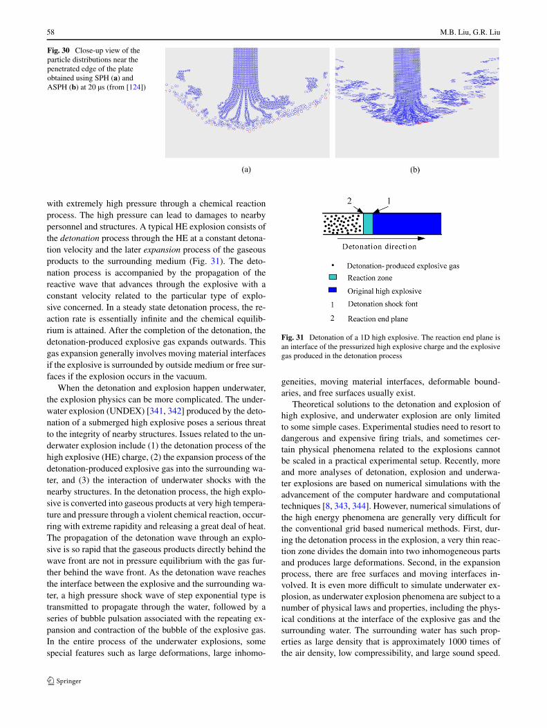
58 M.B. Liu, G.R. Liu
Fig. 30 Close-up view of theparticle distributions near thepenetrated edge of the plateobtained using SPH (a) andASPH (b) at 20 µs (from [124])
with extremely high pressure through a chemical reactionprocess. The high pressure can lead to damages to nearbypersonnel and structures. A typical HE explosion consists ofthe detonation process through the HE at a constant detona-tion velocity and the later expansion process of the gaseousproducts to the surrounding medium (Fig. 31). The deto-nation process is accompanied by the propagation of thereactive wave that advances through the explosive with aconstant velocity related to the particular type of explo-sive concerned. In a steady state detonation process, the re-action rate is essentially infinite and the chemical equilib-rium is attained. After the completion of the detonation, thedetonation-produced explosive gas expands outwards. Thisgas expansion generally involves moving material interfacesif the explosive is surrounded by outside medium or free sur-faces if the explosion occurs in the vacuum.
When the detonation and explosion happen underwater,the explosion physics can be more complicated. The under-water explosion (UNDEX) [341, 342] produced by the deto-nation of a submerged high explosive poses a serious threatto the integrity of nearby structures. Issues related to the un-derwater explosion include (1) the detonation process of thehigh explosive (HE) charge, (2) the expansion process of thedetonation-produced explosive gas into the surrounding wa-ter, and (3) the interaction of underwater shocks with thenearby structures. In the detonation process, the high explo-sive is converted into gaseous products at very high tempera-ture and pressure through a violent chemical reaction, occur-ring with extreme rapidity and releasing a great deal of heat.The propagation of the detonation wave through an explo-sive is so rapid that the gaseous products directly behind thewave front are not in pressure equilibrium with the gas fur-ther behind the wave front. As the detonation wave reachesthe interface between the explosive and the surrounding wa-ter, a high pressure shock wave of step exponential type istransmitted to propagate through the water, followed by aseries of bubble pulsation associated with the repeating ex-pansion and contraction of the bubble of the explosive gas.In the entire process of the underwater explosions, somespecial features such as large deformations, large inhomo-
Fig. 31 Detonation of a 1D high explosive. The reaction end plane isan interface of the pressurized high explosive charge and the explosivegas produced in the detonation process
geneities, moving material interfaces, deformable bound-aries, and free surfaces usually exist.
Theoretical solutions to the detonation and explosion ofhigh explosive, and underwater explosion are only limitedto some simple cases. Experimental studies need to resort todangerous and expensive firing trials, and sometimes cer-tain physical phenomena related to the explosions cannotbe scaled in a practical experimental setup. Recently, moreand more analyses of detonation, explosion and underwa-ter explosions are based on numerical simulations with theadvancement of the computer hardware and computationaltechniques [8, 343, 344]. However, numerical simulations ofthe high energy phenomena are generally very difficult forthe conventional grid based numerical methods. First, dur-ing the detonation process in the explosion, a very thin reac-tion zone divides the domain into two inhomogeneous partsand produces large deformations. Second, in the expansionprocess, there are free surfaces and moving interfaces in-volved. It is even more difficult to simulate underwater ex-plosion, as underwater explosion phenomena are subject to anumber of physical laws and properties, including the phys-ical conditions at the interface of the explosive gas and thesurrounding water. The surrounding water has such prop-erties as large density that is approximately 1000 times ofthe air density, low compressibility, and large sound speed.
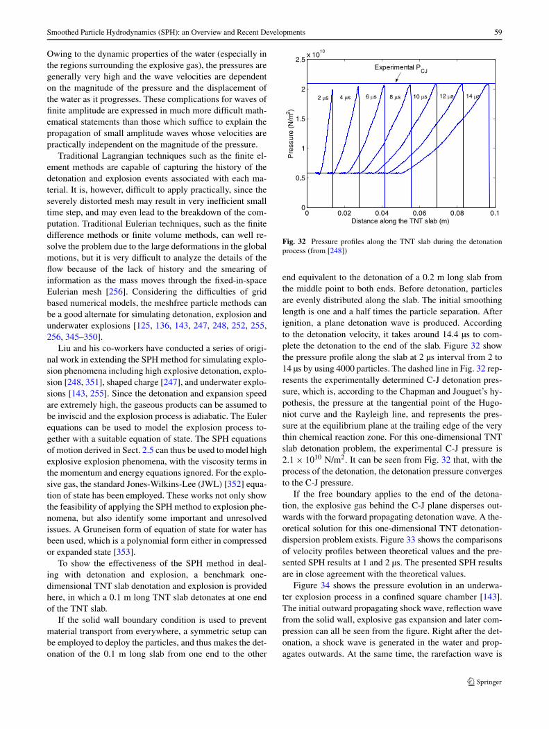
Smoothed Particle Hydrodynamics (SPH): an Overview and Recent Developments 59
Owing to the dynamic properties of the water (especially inthe regions surrounding the explosive gas), the pressures aregenerally very high and the wave velocities are dependenton the magnitude of the pressure and the displacement ofthe water as it progresses. These complications for waves offinite amplitude are expressed in much more difficult math-ematical statements than those which suffice to explain thepropagation of small amplitude waves whose velocities arepractically independent on the magnitude of the pressure.
Traditional Lagrangian techniques such as the finite el-ement methods are capable of capturing the history of thedetonation and explosion events associated with each ma-terial. It is, however, difficult to apply practically, since theseverely distorted mesh may result in very inefficient smalltime step, and may even lead to the breakdown of the com-putation. Traditional Eulerian techniques, such as the finitedifference methods or finite volume methods, can well re-solve the problem due to the large deformations in the globalmotions, but it is very difficult to analyze the details of theflow because of the lack of history and the smearing ofinformation as the mass moves through the fixed-in-spaceEulerian mesh [256]. Considering the difficulties of gridbased numerical models, the meshfree particle methods canbe a good alternate for simulating detonation, explosion andunderwater explosions [125, 136, 143, 247, 248, 252, 255,256, 345–350].
Liu and his co-workers have conducted a series of origi-nal work in extending the SPH method for simulating explo-sion phenomena including high explosive detonation, explo-sion [248, 351], shaped charge [247], and underwater explo-sions [143, 255]. Since the detonation and expansion speedare extremely high, the gaseous products can be assumed tobe inviscid and the explosion process is adiabatic. The Eulerequations can be used to model the explosion process to-gether with a suitable equation of state. The SPH equationsof motion derived in Sect. 2.5 can thus be used to model highexplosive explosion phenomena, with the viscosity terms inthe momentum and energy equations ignored. For the explo-sive gas, the standard Jones-Wilkins-Lee (JWL) [352] equa-tion of state has been employed. These works not only showthe feasibility of applying the SPH method to explosion phe-nomena, but also identify some important and unresolvedissues. A Gruneisen form of equation of state for water hasbeen used, which is a polynomial form either in compressedor expanded state [353].
To show the effectiveness of the SPH method in deal-ing with detonation and explosion, a benchmark one-dimensional TNT slab denotation and explosion is providedhere, in which a 0.1 m long TNT slab detonates at one endof the TNT slab.
If the solid wall boundary condition is used to preventmaterial transport from everywhere, a symmetric setup canbe employed to deploy the particles, and thus makes the det-onation of the 0.1 m long slab from one end to the other
Fig. 32 Pressure profiles along the TNT slab during the detonationprocess (from [248])
end equivalent to the detonation of a 0.2 m long slab fromthe middle point to both ends. Before detonation, particlesare evenly distributed along the slab. The initial smoothinglength is one and a half times the particle separation. Afterignition, a plane detonation wave is produced. Accordingto the detonation velocity, it takes around 14.4 µs to com-plete the detonation to the end of the slab. Figure 32 showthe pressure profile along the slab at 2 µs interval from 2 to14 µs by using 4000 particles. The dashed line in Fig. 32 rep-resents the experimentally determined C-J detonation pres-sure, which is, according to the Chapman and Jouguet’s hy-pothesis, the pressure at the tangential point of the Hugo-niot curve and the Rayleigh line, and represents the pres-sure at the equilibrium plane at the trailing edge of the verythin chemical reaction zone. For this one-dimensional TNTslab detonation problem, the experimental C-J pressure is2.1 × 1010 N/m2. It can be seen from Fig. 32 that, with theprocess of the detonation, the detonation pressure convergesto the C-J pressure.
If the free boundary applies to the end of the detona-tion, the explosive gas behind the C-J plane disperses out-wards with the forward propagating detonation wave. A the-oretical solution for this one-dimensional TNT detonation-dispersion problem exists. Figure 33 shows the comparisonsof velocity profiles between theoretical values and the pre-sented SPH results at 1 and 2 µs. The presented SPH resultsare in close agreement with the theoretical values.
Figure 34 shows the pressure evolution in an underwa-ter explosion process in a confined square chamber [143].The initial outward propagating shock wave, reflection wavefrom the solid wall, explosive gas expansion and later com-pression can all be seen from the figure. Right after the det-onation, a shock wave is generated in the water and prop-agates outwards. At the same time, the rarefaction wave is
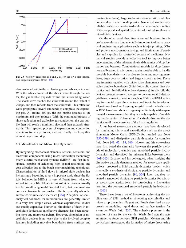
60 M.B. Liu, G.R. Liu
Fig. 33 Velocity transients at 1 and 2 µs for the TNT slab detona-tion-dispersion process (from [248])
also produced within the explosive gas and advances inward.With the advancement of the shock wave through the wa-ter, the gas bubble expands within the surrounding water.The shock wave reaches the solid wall around the instant of200 µs, and then reflects from the solid wall. This reflectionwave propagates inward and tends to compress the expand-ing gas. At around 400 µs, the gas bubble reaches to themaximum and then reduces. With the continued process ofshock reflection and explosive gas contraction, the gas bub-ble then will reach a minimum size, and then expands after-wards. This repeated process of expansion and contractionmaintains for many circles, and will finally reach equilib-rium at larger time step.
6.3 Microfluidics and Micro Drop Dynamics
By integrating mechanical elements, sensors, actuators, andelectronic components using micro-fabrication technology,micro-electro-mechanical systems (MEMS) are fast in re-sponse, capable of achieving high spatial resolution, andcost-effective due to the batch micromachining techniques.Characterization of fluid flows in microfluidic devices hasincreasingly becoming a very important topic since the flu-idic behavior in MEMS is very different from what ob-served in daily life. Flows in microfluidic devices usuallyinvolve small or ignorable inertial force, but dominant vis-cous, electro-kinetic and surface effects especially when thesurface-to-volume ratio increases [354]. Analytical or semi-analytical solutions for microfluidics are generally limitedto a very few simple cases, whereas experimental studiesare usually expensive. Numerical simulation of flows in mi-crofluidic devices, as an effective alternate, has been attract-ing more and more researchers. However, simulation of mi-crofluidic devices is not easy due to the involved complexfeatures including movable boundaries (free surfaces and
moving interfaces), large surface-to-volume ratio, and phe-nomena due to micro scale physics. Numerical studies withreliable models are needed to develop a better understandingof the temporal and spatial dynamics of multiphase flows inmicrofluidic devices.
On the other hand, drop formation and break-up in mi-cro/nano scales are fundamentally important to diverse prac-tical engineering applications such as ink-jet printing, DNAand protein micro-/nano-arraying, and fabrication of parti-cles and capsules for controlled release of medicines. Nu-merical studies provide an effective tool to improve betterunderstanding of the inherent physical dynamics of drop for-mation and breakup. Computational models for drop forma-tion and breakup in micro/nano scales must be able to handlemovable boundaries such as free surfaces and moving inter-faces, large density ratios, and large viscosity ratios. Theserequirements together with micro scale phenomena and pos-sible complex boundaries (fluid-fluid-solid contact line dy-namics and fluid-fluid interface dynamics) in microfluidicdevices present severe challenges to conventional Eulerian-grid based numerical methods such as FDM and FVM whichrequire special algorithms to treat and track the interfaces.Algorithms based on Lagrangian-grid based methods suchas FEM have been shown to agree quantitatively with exper-imental measurements, but they are only capable of model-ing the dynamics of formation of a single drop or the dy-namics until the occurrence of the first singularity.
A number of meso-scale methods have been developedfor simulating micro- and nano-fluidics such as the directsimulation Monte Carlo (DSMC) for rarefied gas flows[355–359], and dissipative particle dynamics for complexfluid flows [41, 42, 118, 360]. Hoover and his co-workershave first noted the similarity between the particle meth-ods of molecular dynamics and smoothed particle hydro-dynamics, and described the inherent links between them[361–363]. Espanol and his colleagues, when studying thedissipative particle dynamics method for meso-scale appli-cations, proposed a fluid particle dynamics model, whichis actually a synthesis of dissipative particle dynamics andsmoothed particle dynamics [96, 364]. Later on, they in-vented a smoothed dissipative particle dynamics for micro-or meso-scale applications, by introducing a fluctuationterm into the conventional smoothed particle hydrodynam-ics [365].
There have been a lot of literatures addressing the ap-plications of SPH method to simulating microfluidics andmicro drop dynamics. Nugent and Posch described an ap-proach to modeling liquid drops and surface tension fora van der Waals fluid [236]. The cohesive pressure in theequation of state for the van der Waals fluid actually actsan attractive force between SPH particles. Melean and hisco-workers investigated the formation of micro drops using
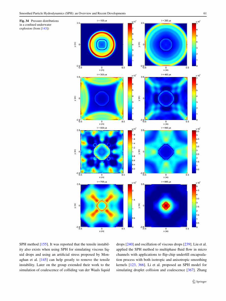
Smoothed Particle Hydrodynamics (SPH): an Overview and Recent Developments 61
Fig. 34 Pressure distributionsin a confined underwaterexplosion (from [143])
SPH method [155]. It was reported that the tensile instabil-ity also exists when using SPH for simulating viscous liq-uid drops and using an artificial stress proposed by Mon-aghan et al. [145] can help greatly to remove the tensileinstability. Later on the group extended their work to thesimulation of coalescence of colliding van der Waals liquid
drops [240] and oscillation of viscous drops [239]. Liu et al.applied the SPH method to multiphase fluid flow in microchannels with applications to flip-chip underfill encapsula-tion process with both isotropic and anisotropic smoothingkernels [123, 366]. Li et al. proposed an SPH model forsimulating droplet collision and coalescence [367]. Zhang
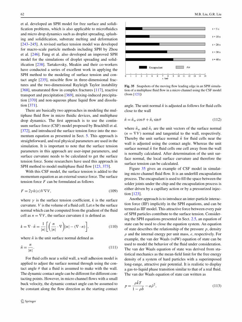
62 M.B. Liu, G.R. Liu
et al. developed an SPH model for free surface and solidi-fication problems, which is also applicable to microfluidicsand micro drop dynamics such as droplet spreading, splash-ing and solidification, substrate melting and deformation[243–245]. A revised surface tension model was developedfor macro-scale particle methods including SPH by Zhouet al. [246]. Fang et al. also developed an improved SPHmodel for the simulations of droplet spreading and solid-ification [238]. Tartakovsky, Meakin and their co-workershave conducted a series of excellent work in applying theSPH method to the modeling of surface tension and con-tact angle [235], miscible flow in three-dimensional frac-tures and the two-dimensional Rayleigh Taylor instability[368], unsaturated flow in complex fractures [117], reactivetransport and precipitation [369], mixing-induced precipita-tion [370] and non-aqueous phase liquid flow and dissolu-tion [371].
There are basically two approaches in modeling the mul-tiphase fluid flow in micro fluidic devices, and multiphasedrop dynamics. The first approach is to use the contin-uum surface force (CSF) model proposed by Brackbill et al.[372], and introduced the surface tension force into the mo-mentum equation as presented in Sect. 5. This approach isstraightforward, and real physical parameters are used in thesimulation. It is important to note that the surface tensionparameters in this approach are user-input parameters, andsurface curvature needs to be calculated to get the surfacetension force. Some researchers have used this approach inSPH method to model multiphase fluid flow [123, 373].
With this CSF model, the surface tension is added to themomentum equation as an external source force. The surfacetension force F can be formulated as follows
F = 2γ k(x)V ∇V, (109)
where γ is the surface tension coefficient, k is the surfacecurvature. V is the volume of a fluid cell. Let n be the surfacenormal which can be computed from the gradient of the fluidcell as n = ∇V , the surface curvature k is defined as
k = ∇ · n = 1
|n|[(
n
|n| · ∇)
|n| − (∇ · n)
], (110)
where n is the unit surface normal defined as
n = n
|n| . (111)
For fluid cells near a solid wall, a wall adhesion model isapplied to adjust the surface normal through using the con-tact angle θ that a fluid is assumed to make with the wall.The dynamic contact angle can be different for different con-tacting points. However, in micro channel flows with a smallbuck velocity, the dynamic contact angle can be assumed tobe constant along the flow direction as the starting contact
Fig. 35 Snapshots of the moving flow leading edge in an SPH simula-tion of a multiphase fluid flow in a micro channel using the CSF model(from [123])
angle. The unit normal n is adjusted as follows for fluid cellsclose to the wall
n = nw cos θ + nt sin θ (112)
where nw and nt are the unit vectors of the surface normal(n = ∇V ) normal and tangential to the wall, respectively.Thereby the unit surface normal n for fluid cells near thewall is adjusted using the contact angle. Whereas the unitsurface normal n for fluid cells one cell away from the wallis normally calculated. After determination of the unit sur-face normal, the local surface curvature and therefore thesurface tension can be calculated.
Figure 35 gives an example of CSF model in simulat-ing micro channel fluid flow. It is an underfill encapsulationprocess. The encapsulant is used to fill the space between thesolder joints under the chip and the encapsulation process iseither driven by a capillary action or by a pressurized injec-tion [123].
Another approach is to introduce an inter-particle interac-tion force (IIF) implicitly in the SPH equations, and can betermed as IIF model. This attractive force between every pairof SPH particles contribute to the surface tension. Consider-ing the SPH equations presented in Sect. 2.5, an equation ofstate can be used to close the equation system. An equationof state describes the relationship of the pressure p, densityρ and the internal energy per unit mass, e, respectively. Forexample, the van der Waals (vdW) equation of state can beused to model the behavior of the fluid under consideration.The van der Waals equation of state was derived from sta-tistical mechanics as the mean-field limit for the free energydensity of a system of hard particles with a superimposedlong-range, attractive pair potential. It is realistic to displaya gas-to-liquid phase transition similar to that of a real fluid.The van der Waals equation of state can written as
p = ρkT
1 − ρb− aρ2, (113)
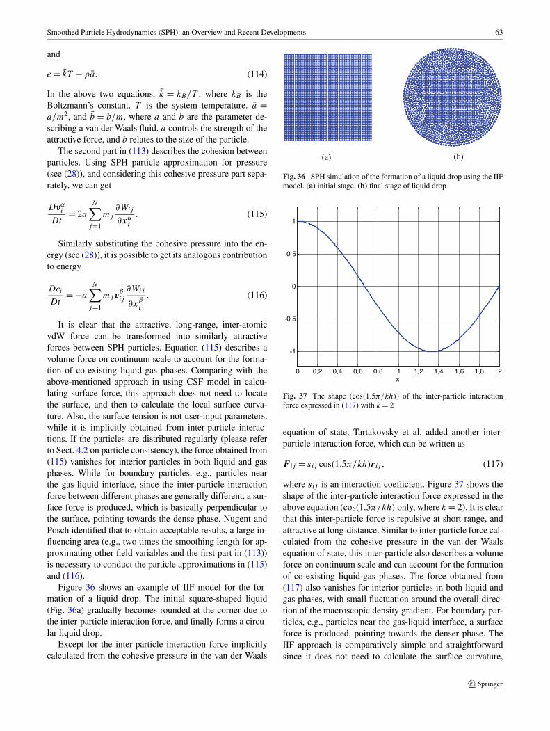
Smoothed Particle Hydrodynamics (SPH): an Overview and Recent Developments 63
and
e = kT − ρa. (114)
In the above two equations, k = kB/T , where kB is theBoltzmann’s constant. T is the system temperature. a =a/m2, and b = b/m, where a and b are the parameter de-scribing a van der Waals fluid. a controls the strength of theattractive force, and b relates to the size of the particle.
The second part in (113) describes the cohesion betweenparticles. Using SPH particle approximation for pressure(see (28)), and considering this cohesive pressure part sepa-rately, we can get
Dvαi
Dt= 2a
N∑j=1
mj
∂Wij
∂xαi
. (115)
Similarly substituting the cohesive pressure into the en-ergy (see (28)), it is possible to get its analogous contributionto energy
Dei
Dt= −a
N∑j=1
mjvβij
∂Wij
∂xβi
. (116)
It is clear that the attractive, long-range, inter-atomicvdW force can be transformed into similarly attractiveforces between SPH particles. Equation (115) describes avolume force on continuum scale to account for the forma-tion of co-existing liquid-gas phases. Comparing with theabove-mentioned approach in using CSF model in calcu-lating surface force, this approach does not need to locatethe surface, and then to calculate the local surface curva-ture. Also, the surface tension is not user-input parameters,while it is implicitly obtained from inter-particle interac-tions. If the particles are distributed regularly (please referto Sect. 4.2 on particle consistency), the force obtained from(115) vanishes for interior particles in both liquid and gasphases. While for boundary particles, e.g., particles nearthe gas-liquid interface, since the inter-particle interactionforce between different phases are generally different, a sur-face force is produced, which is basically perpendicular tothe surface, pointing towards the dense phase. Nugent andPosch identified that to obtain acceptable results, a large in-fluencing area (e.g., two times the smoothing length for ap-proximating other field variables and the first part in (113))is necessary to conduct the particle approximations in (115)and (116).
Figure 36 shows an example of IIF model for the for-mation of a liquid drop. The initial square-shaped liquid(Fig. 36a) gradually becomes rounded at the corner due tothe inter-particle interaction force, and finally forms a circu-lar liquid drop.
Except for the inter-particle interaction force implicitlycalculated from the cohesive pressure in the van der Waals
Fig. 36 SPH simulation of the formation of a liquid drop using the IIFmodel. (a) initial stage, (b) final stage of liquid drop
Fig. 37 The shape (cos(1.5π/kh)) of the inter-particle interactionforce expressed in (117) with k = 2
equation of state, Tartakovsky et al. added another inter-particle interaction force, which can be written as
F ij = sij cos(1.5π/kh)r ij , (117)
where sij is an interaction coefficient. Figure 37 shows theshape of the inter-particle interaction force expressed in theabove equation (cos(1.5π/kh) only, where k = 2). It is clearthat this inter-particle force is repulsive at short range, andattractive at long-distance. Similar to inter-particle force cal-culated from the cohesive pressure in the van der Waalsequation of state, this inter-particle also describes a volumeforce on continuum scale and can account for the formationof co-existing liquid-gas phases. The force obtained from(117) also vanishes for interior particles in both liquid andgas phases, with small fluctuation around the overall direc-tion of the macroscopic density gradient. For boundary par-ticles, e.g., particles near the gas-liquid interface, a surfaceforce is produced, pointing towards the denser phase. TheIIF approach is comparatively simple and straightforwardsince it does not need to calculate the surface curvature,
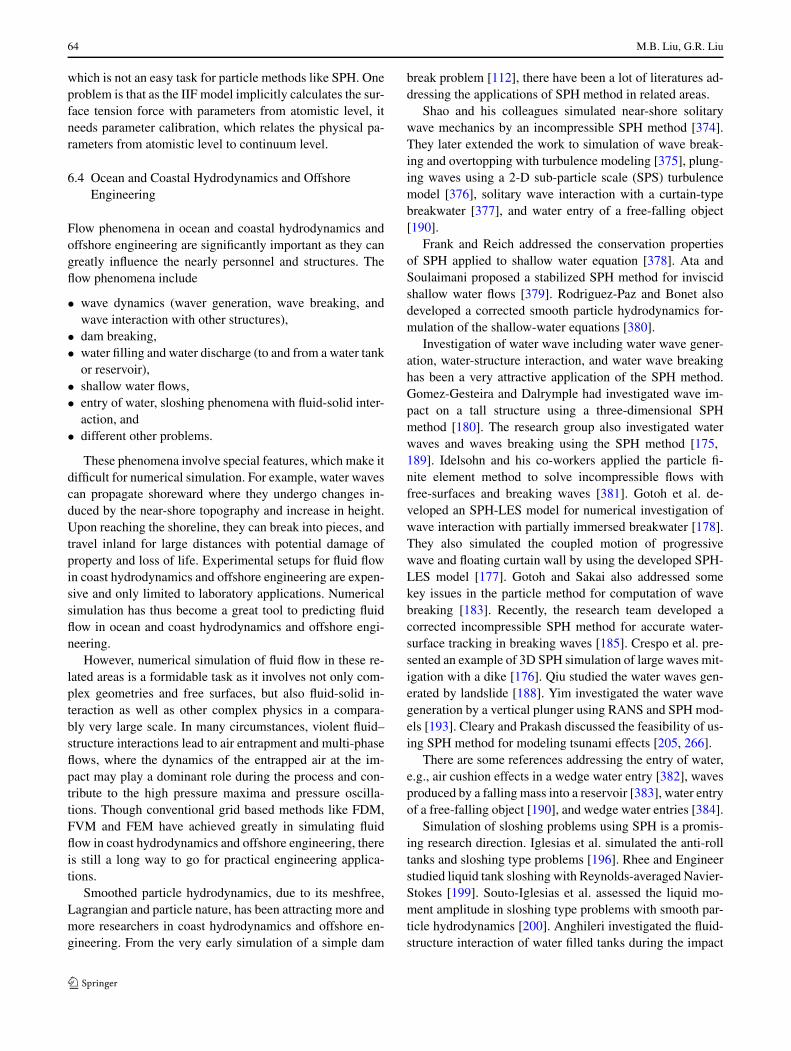
64 M.B. Liu, G.R. Liu
which is not an easy task for particle methods like SPH. Oneproblem is that as the IIF model implicitly calculates the sur-face tension force with parameters from atomistic level, itneeds parameter calibration, which relates the physical pa-rameters from atomistic level to continuum level.
6.4 Ocean and Coastal Hydrodynamics and OffshoreEngineering
Flow phenomena in ocean and coastal hydrodynamics andoffshore engineering are significantly important as they cangreatly influence the nearly personnel and structures. Theflow phenomena include
• wave dynamics (waver generation, wave breaking, andwave interaction with other structures),
• dam breaking,• water filling and water discharge (to and from a water tank
or reservoir),• shallow water flows,• entry of water, sloshing phenomena with fluid-solid inter-
action, and• different other problems.
These phenomena involve special features, which make itdifficult for numerical simulation. For example, water wavescan propagate shoreward where they undergo changes in-duced by the near-shore topography and increase in height.Upon reaching the shoreline, they can break into pieces, andtravel inland for large distances with potential damage ofproperty and loss of life. Experimental setups for fluid flowin coast hydrodynamics and offshore engineering are expen-sive and only limited to laboratory applications. Numericalsimulation has thus become a great tool to predicting fluidflow in ocean and coast hydrodynamics and offshore engi-neering.
However, numerical simulation of fluid flow in these re-lated areas is a formidable task as it involves not only com-plex geometries and free surfaces, but also fluid-solid in-teraction as well as other complex physics in a compara-bly very large scale. In many circumstances, violent fluid–structure interactions lead to air entrapment and multi-phaseflows, where the dynamics of the entrapped air at the im-pact may play a dominant role during the process and con-tribute to the high pressure maxima and pressure oscilla-tions. Though conventional grid based methods like FDM,FVM and FEM have achieved greatly in simulating fluidflow in coast hydrodynamics and offshore engineering, thereis still a long way to go for practical engineering applica-tions.
Smoothed particle hydrodynamics, due to its meshfree,Lagrangian and particle nature, has been attracting more andmore researchers in coast hydrodynamics and offshore en-gineering. From the very early simulation of a simple dam
break problem [112], there have been a lot of literatures ad-dressing the applications of SPH method in related areas.
Shao and his colleagues simulated near-shore solitarywave mechanics by an incompressible SPH method [374].They later extended the work to simulation of wave break-ing and overtopping with turbulence modeling [375], plung-ing waves using a 2-D sub-particle scale (SPS) turbulencemodel [376], solitary wave interaction with a curtain-typebreakwater [377], and water entry of a free-falling object[190].
Frank and Reich addressed the conservation propertiesof SPH applied to shallow water equation [378]. Ata andSoulaimani proposed a stabilized SPH method for inviscidshallow water flows [379]. Rodriguez-Paz and Bonet alsodeveloped a corrected smooth particle hydrodynamics for-mulation of the shallow-water equations [380].
Investigation of water wave including water wave gener-ation, water-structure interaction, and water wave breakinghas been a very attractive application of the SPH method.Gomez-Gesteira and Dalrymple had investigated wave im-pact on a tall structure using a three-dimensional SPHmethod [180]. The research group also investigated waterwaves and waves breaking using the SPH method [175,189]. Idelsohn and his co-workers applied the particle fi-nite element method to solve incompressible flows withfree-surfaces and breaking waves [381]. Gotoh et al. de-veloped an SPH-LES model for numerical investigation ofwave interaction with partially immersed breakwater [178].They also simulated the coupled motion of progressivewave and floating curtain wall by using the developed SPH-LES model [177]. Gotoh and Sakai also addressed somekey issues in the particle method for computation of wavebreaking [183]. Recently, the research team developed acorrected incompressible SPH method for accurate water-surface tracking in breaking waves [185]. Crespo et al. pre-sented an example of 3D SPH simulation of large waves mit-igation with a dike [176]. Qiu studied the water waves gen-erated by landslide [188]. Yim investigated the water wavegeneration by a vertical plunger using RANS and SPH mod-els [193]. Cleary and Prakash discussed the feasibility of us-ing SPH method for modeling tsunami effects [205, 266].
There are some references addressing the entry of water,e.g., air cushion effects in a wedge water entry [382], wavesproduced by a falling mass into a reservoir [383], water entryof a free-falling object [190], and wedge water entries [384].
Simulation of sloshing problems using SPH is a promis-ing research direction. Iglesias et al. simulated the anti-rolltanks and sloshing type problems [196]. Rhee and Engineerstudied liquid tank sloshing with Reynolds-averaged Navier-Stokes [199]. Souto-Iglesias et al. assessed the liquid mo-ment amplitude in sloshing type problems with smooth par-ticle hydrodynamics [200]. Anghileri investigated the fluid-structure interaction of water filled tanks during the impact
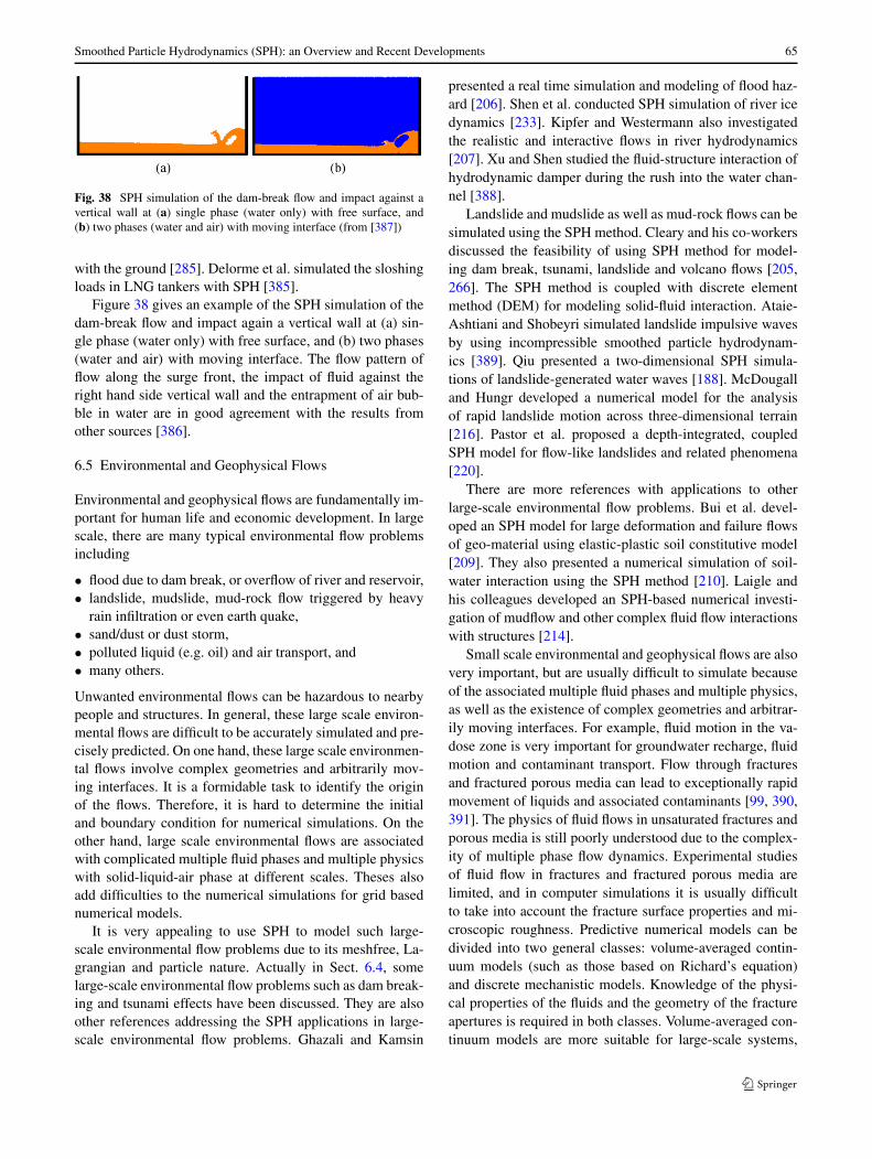
Smoothed Particle Hydrodynamics (SPH): an Overview and Recent Developments 65
Fig. 38 SPH simulation of the dam-break flow and impact against avertical wall at (a) single phase (water only) with free surface, and(b) two phases (water and air) with moving interface (from [387])
with the ground [285]. Delorme et al. simulated the sloshingloads in LNG tankers with SPH [385].
Figure 38 gives an example of the SPH simulation of thedam-break flow and impact again a vertical wall at (a) sin-gle phase (water only) with free surface, and (b) two phases(water and air) with moving interface. The flow pattern offlow along the surge front, the impact of fluid against theright hand side vertical wall and the entrapment of air bub-ble in water are in good agreement with the results fromother sources [386].
6.5 Environmental and Geophysical Flows
Environmental and geophysical flows are fundamentally im-portant for human life and economic development. In largescale, there are many typical environmental flow problemsincluding
• flood due to dam break, or overflow of river and reservoir,• landslide, mudslide, mud-rock flow triggered by heavy
rain infiltration or even earth quake,• sand/dust or dust storm,• polluted liquid (e.g. oil) and air transport, and• many others.
Unwanted environmental flows can be hazardous to nearbypeople and structures. In general, these large scale environ-mental flows are difficult to be accurately simulated and pre-cisely predicted. On one hand, these large scale environmen-tal flows involve complex geometries and arbitrarily mov-ing interfaces. It is a formidable task to identify the originof the flows. Therefore, it is hard to determine the initialand boundary condition for numerical simulations. On theother hand, large scale environmental flows are associatedwith complicated multiple fluid phases and multiple physicswith solid-liquid-air phase at different scales. Theses alsoadd difficulties to the numerical simulations for grid basednumerical models.
It is very appealing to use SPH to model such large-scale environmental flow problems due to its meshfree, La-grangian and particle nature. Actually in Sect. 6.4, somelarge-scale environmental flow problems such as dam break-ing and tsunami effects have been discussed. They are alsoother references addressing the SPH applications in large-scale environmental flow problems. Ghazali and Kamsin
presented a real time simulation and modeling of flood haz-ard [206]. Shen et al. conducted SPH simulation of river icedynamics [233]. Kipfer and Westermann also investigatedthe realistic and interactive flows in river hydrodynamics[207]. Xu and Shen studied the fluid-structure interaction ofhydrodynamic damper during the rush into the water chan-nel [388].
Landslide and mudslide as well as mud-rock flows can besimulated using the SPH method. Cleary and his co-workersdiscussed the feasibility of using SPH method for model-ing dam break, tsunami, landslide and volcano flows [205,266]. The SPH method is coupled with discrete elementmethod (DEM) for modeling solid-fluid interaction. Ataie-Ashtiani and Shobeyri simulated landslide impulsive wavesby using incompressible smoothed particle hydrodynam-ics [389]. Qiu presented a two-dimensional SPH simula-tions of landslide-generated water waves [188]. McDougalland Hungr developed a numerical model for the analysisof rapid landslide motion across three-dimensional terrain[216]. Pastor et al. proposed a depth-integrated, coupledSPH model for flow-like landslides and related phenomena[220].
There are more references with applications to otherlarge-scale environmental flow problems. Bui et al. devel-oped an SPH model for large deformation and failure flowsof geo-material using elastic-plastic soil constitutive model[209]. They also presented a numerical simulation of soil-water interaction using the SPH method [210]. Laigle andhis colleagues developed an SPH-based numerical investi-gation of mudflow and other complex fluid flow interactionswith structures [214].
Small scale environmental and geophysical flows are alsovery important, but are usually difficult to simulate becauseof the associated multiple fluid phases and multiple physics,as well as the existence of complex geometries and arbitrar-ily moving interfaces. For example, fluid motion in the va-dose zone is very important for groundwater recharge, fluidmotion and contaminant transport. Flow through fracturesand fractured porous media can lead to exceptionally rapidmovement of liquids and associated contaminants [99, 390,391]. The physics of fluid flows in unsaturated fractures andporous media is still poorly understood due to the complex-ity of multiple phase flow dynamics. Experimental studiesof fluid flow in fractures and fractured porous media arelimited, and in computer simulations it is usually difficultto take into account the fracture surface properties and mi-croscopic roughness. Predictive numerical models can bedivided into two general classes: volume-averaged contin-uum models (such as those based on Richard’s equation)and discrete mechanistic models. Knowledge of the physi-cal properties of the fluids and the geometry of the fractureapertures is required in both classes. Volume-averaged con-tinuum models are more suitable for large-scale systems,
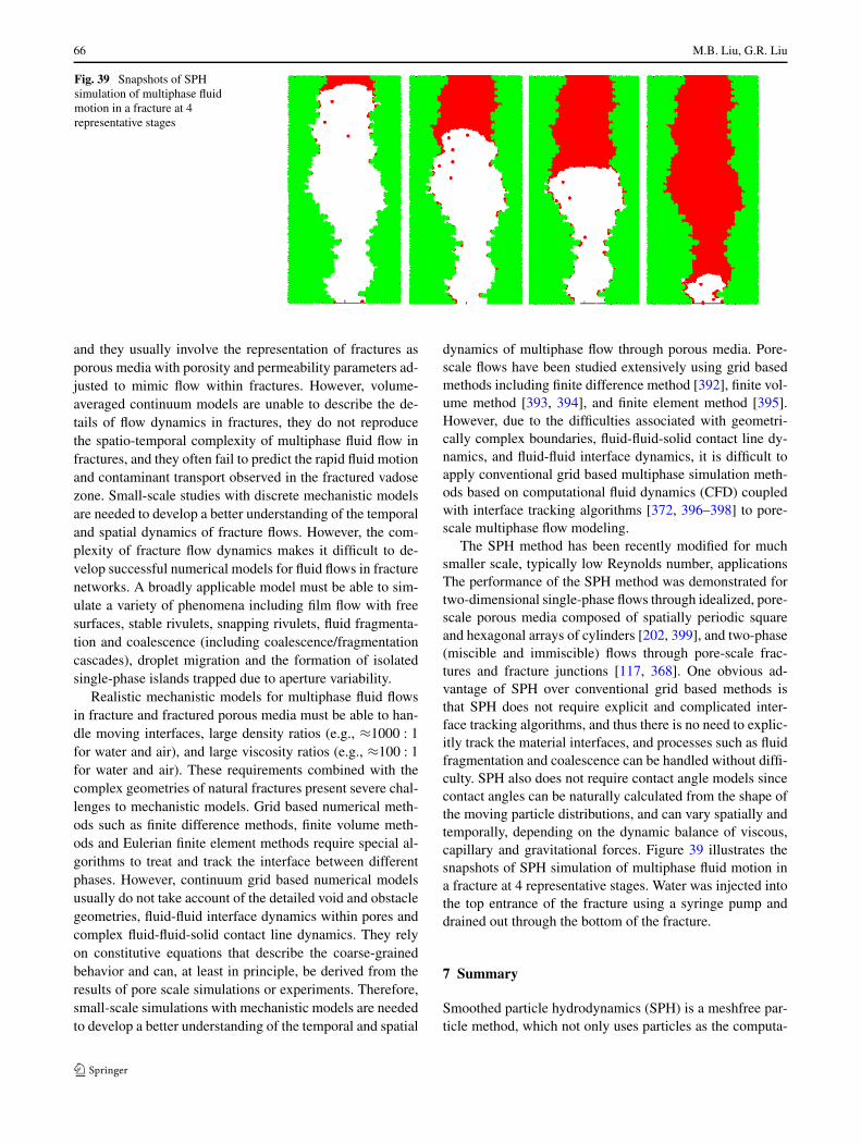
66 M.B. Liu, G.R. Liu
Fig. 39 Snapshots of SPHsimulation of multiphase fluidmotion in a fracture at 4representative stages
and they usually involve the representation of fractures asporous media with porosity and permeability parameters ad-justed to mimic flow within fractures. However, volume-averaged continuum models are unable to describe the de-tails of flow dynamics in fractures, they do not reproducethe spatio-temporal complexity of multiphase fluid flow infractures, and they often fail to predict the rapid fluid motionand contaminant transport observed in the fractured vadosezone. Small-scale studies with discrete mechanistic modelsare needed to develop a better understanding of the temporaland spatial dynamics of fracture flows. However, the com-plexity of fracture flow dynamics makes it difficult to de-velop successful numerical models for fluid flows in fracturenetworks. A broadly applicable model must be able to sim-ulate a variety of phenomena including film flow with freesurfaces, stable rivulets, snapping rivulets, fluid fragmenta-tion and coalescence (including coalescence/fragmentationcascades), droplet migration and the formation of isolatedsingle-phase islands trapped due to aperture variability.
Realistic mechanistic models for multiphase fluid flowsin fracture and fractured porous media must be able to han-dle moving interfaces, large density ratios (e.g., ≈1000 : 1for water and air), and large viscosity ratios (e.g., ≈100 : 1for water and air). These requirements combined with thecomplex geometries of natural fractures present severe chal-lenges to mechanistic models. Grid based numerical meth-ods such as finite difference methods, finite volume meth-ods and Eulerian finite element methods require special al-gorithms to treat and track the interface between differentphases. However, continuum grid based numerical modelsusually do not take account of the detailed void and obstaclegeometries, fluid-fluid interface dynamics within pores andcomplex fluid-fluid-solid contact line dynamics. They relyon constitutive equations that describe the coarse-grainedbehavior and can, at least in principle, be derived from theresults of pore scale simulations or experiments. Therefore,small-scale simulations with mechanistic models are neededto develop a better understanding of the temporal and spatial
dynamics of multiphase flow through porous media. Pore-scale flows have been studied extensively using grid basedmethods including finite difference method [392], finite vol-ume method [393, 394], and finite element method [395].However, due to the difficulties associated with geometri-cally complex boundaries, fluid-fluid-solid contact line dy-namics, and fluid-fluid interface dynamics, it is difficult toapply conventional grid based multiphase simulation meth-ods based on computational fluid dynamics (CFD) coupledwith interface tracking algorithms [372, 396–398] to pore-scale multiphase flow modeling.
The SPH method has been recently modified for muchsmaller scale, typically low Reynolds number, applicationsThe performance of the SPH method was demonstrated fortwo-dimensional single-phase flows through idealized, pore-scale porous media composed of spatially periodic squareand hexagonal arrays of cylinders [202, 399], and two-phase(miscible and immiscible) flows through pore-scale frac-tures and fracture junctions [117, 368]. One obvious ad-vantage of SPH over conventional grid based methods isthat SPH does not require explicit and complicated inter-face tracking algorithms, and thus there is no need to explic-itly track the material interfaces, and processes such as fluidfragmentation and coalescence can be handled without diffi-culty. SPH also does not require contact angle models sincecontact angles can be naturally calculated from the shape ofthe moving particle distributions, and can vary spatially andtemporally, depending on the dynamic balance of viscous,capillary and gravitational forces. Figure 39 illustrates thesnapshots of SPH simulation of multiphase fluid motion ina fracture at 4 representative stages. Water was injected intothe top entrance of the fracture using a syringe pump anddrained out through the bottom of the fracture.
7 Summary
Smoothed particle hydrodynamics (SPH) is a meshfree par-ticle method, which not only uses particles as the computa-
Smoothed Particle Hydrodynamics (SPH): an Overview and Recent Developments 67
tional frame for interpolation or differencing, but also usesthe particles to carry the material properties. In this sur-vey, the smoothed particle hydrodynamics method, and itsrecent development in numerical algorithms and applica-tions have been reviewed. In methodology and numericalapproximation, the basic concepts of kernel and particle ap-proximations as well as different techniques for developingSPH formulations have been addressed. Different smooth-ing kernel functions have been reviewed with constructingconditions provided. The emphasis is on the consistencyproblem, which traditionally limits the accuracy of the SPHmethod. A number of consistency restoring approaches havebeen surveyed. An SPH formulation for discontinuity, a gen-eral approach for restoring particle consistency, and a finiteparticle method are described. Several important numericaltopics have been investigated, including (1) solid boundarytreatment, (2) representation of solid obstacles, (3) mater-ial interface treatment and (4) tensile instability. In applica-tions, different applications of the SPH mEthod have beenreviewed, with emphasis on (1) high strain hydrodynamicswith material strength, (2) high explosive detonation and ex-plosions, and underwater explosion, (3) microfluidics andmicro drop dynamics, (4) coast hydrodynamics and offshoreengineering, and (5) environmental and geophysical flows.
The last decades have witnessed the great success of SPHdevelopments in methodology and applications, and thereare still many tasks and challenges remaining. To achievea reliable solution, the computational accuracy, consistency,efficiency, stability and convergence need to be incorporatedinto good SPH algorithms.
In general, SPH has great potential in many problems inengineering and science. It has salient advantages over tra-ditional grid based numerical models in treating large defor-mation, tracking free surfaces, moving interfaces, and de-formable boundaries, resolving moving discontinuities suchas cracks and shock waves. The attraction of the SPHmethod has been showcased in diversified applications, asreviewed in Sect. 7.
One obvious advantage is that the SPH method providesa feasible physical model for non-continuum, as it has somesame features as the classic molecular dynamics methodand the dissipative particle dynamics method. Therefore itwould be very attractive to apply the SPH method to simu-lating problems where the main concern of the object is a setof discrete physical particles rather than a continuum, e.g.,the interaction of stars in astrophysics, movement of mil-lions of atoms in an equilibrium or non-equilibrium state,dynamic behavior of protein molecules, and environmen-tal flows with solid and fluid particles such as landslide andmudslide. There is no need for discretization to begin withfor such situations. Also since SPH shares many similari-ties with other particle methods such as MD and DPD, it isnatural to couple these three methods, from molecular dy-namics (at nano- and micro-scales), to dissipative particle
dynamics (at meso-scales), and then to smoothed particlehydrodynamics (at macro-scales) for simulations with mul-tiple scale physics. It is attractive to develop reliable modelsof length scale coupling for problems with multiple physicsand multiple scales, such as ink-jet printing, DNA and pro-tein micro-/nano-arraying, and fabrication of particles andcapsules for controlled release of medicines.
Acknowledgements The first author, M.B. Liu, has been supportedby the National Natural Science Foundation of China (NSFC Grant No.10942004).
References
1. Chung TJ (2002) Computational fluid dynamics. CambridgeUniversity Press, Cambridge
2. Anderson JD (2002) Computational fluid dynamics: the basicswith applications. McGraw Hill, New York
3. Zienkiewicz OC, Taylor RL (2000) The finite element method.Butterworth-Heinemann, Stonham
4. Liu GR (2002) Meshfree methods: moving beyond the finite ele-ment method. CRC Press, Boca Raton
5. Hirsch C (1988) Numerical computation of internal & exter-nal flows: fundamentals of numerical discretization. Wiley, NewYork
6. Liu GR, Liu MB (2003) Smoothed particle hydrodynamics: ameshfree particle method. World Scientific, Singapore
7. Liu GR, Gu YT (2005) An Introduction to meshfree methods andtheir programming. Springer, Dordrecht, p 479
8. Zhang SZ (1976) Detonation and its applications. Press of Na-tional Defense Industry, Beijing
9. Zukas JA (1990) High velocity impact dynamics. Wiley, NewYork
10. Hockney RW, Eastwood JW (1988) Computer simulation usingparticles. Institute of Physics Publishing, Bristol
11. Allen MP, Tildesley DJ (1987) Computer simulation of liquids.Oxford University Press, Oxford
12. Li S, Liu WK (2002) Meshfree and particle methods and theirapplications. Appl Mech Rev 55(1):1–34
13. Belytschko T, Krongauz Y, Organ D, Fleming M, Krysl P (1996)Meshless methods: an overview and recent developments. Com-put Methods Appl Mech Eng 139(1–4):3–47
14. Idelsohn SR, Onate E (2006) To mesh or not to mesh? That is thequestion. Comput Methods Appl Mech Eng 195(37–40):4681–4696
15. Nguyen VP, Rabczuk T, Bordas S, Duflot M (2008) Meshlessmethods: a review and computer implementation aspects. MathComput Simul 79(3):763–813
16. Liu GR (2008) A generalized Gradient smoothing techniqueand the smoothed bilinear form for Galerkin formulation of awide class of computational methods. Int J Comput Methods5(2):199–236
17. Liu GR (2009) A G space theory and weakened weak (W2) formfor a unified formulation of compatible and incompatible meth-ods, part I: theory. Int J Numer Methods Eng. doi:10.1002/nme.2719
18. Liu GR (2009) A G space theory and weakened weak (W2) formfor a unified formulation of compatible and incompatible meth-ods, part II: applications to solid mechanics problems. Int J Nu-mer Methods Eng. doi:10.1002/nme.2720
19. Liu GR (2009) On the G space theory. Int J Comput Methods6(2):257–289
68 M.B. Liu, G.R. Liu
20. Liu GR, Nguyen-Thoi T, H. N-X, Lam KY (2008) A node-basedsmoothed finite element method (NS-FEM) for upper bound so-lutions to solid mechanics problems. Comput Struct 87:14–26
21. Liu GR, Zhang GY (2008) Upper bound solution to elastic-ity problems: a unique property of the linearly conformingpoint interpolation method (LC-PIM). Int J Numer Methods Eng74:1128–1161
22. Liu GR, Nguyen-Thoi T, Lam KY (2009) An edge-basedsmoothed finite element method (ES-FEM) for static, free andforced vibration analyses in solids. J Sound Vib 320:1100–1130
23. Zhang GY, Liu GR, Nguyen TT, Song CX, Han X, Zhong ZH,Li GY (2007) The upper bound property for solid mechanics ofthe linearly conforming radial point interpolation method (LC-RPIM). Int J Comput Methods 4(3):521–541
24. Liu GR, Zhang GY (2009) A normed G space and weakenedweak (W2) formulation of a cell-based smoothed point interpo-lation method. Int J Comput Methods 6(1):147–179
25. Liu GR, Zhang GY (2008) Edge-based Smoothed Point Interpo-lation Methods. Int J Comput Methods 5(4):621–646
26. Liu GY, Zhang GY (2009) A novel scheme of strain-constructedpoint interpolation method for static and dynamic mechanicsproblems. Int J Appl Mech 1(1):233–258
27. Liu GR, Xu X, Zhang GY, Nguyen-Thoi T (2009) A supercon-vergent point interpolation method (SC-PIM) with piecewise lin-ear strain field using triangular mesh. Int J Numer Methods Eng77:1439–1467
28. Liu GR, Xu X, Zhang GY, Gu YT (2009) An extended Galerkinweak form and a point interpolation method with continuousstrain field and superconvergence using triangular mesh. Com-put Mech 43:651–673
29. Nguyen-Thoi T, Liu GR, Lam KY, Zhang GY (2009) A face-based smoothed finite element method (FS-FEM) for 3D linearand nonlinear solid mechanics problems using 4-node tetrahedralelements. Int J Numer Methods Eng 78:324–353
30. Liu GR, Nguyen-Thoi T, Lam KY (2008) A novel Alpha finiteelement method (FEM) for exact solution to mechanics problemsusing triangular and tetrahedral elements. Comput Methods ApplMech Eng 197:3883–3897
31. Liu GR, Nguyen-Xuan H, Nguyen TT, Xu X (2009) A novelweak form and a superconvergent alpha finite element methodfor mechanics problems using triangular meshes. J Comput Phys228(11):3911–4302
32. Liu GR, Zhang J, Lam KY (2008) A gradient smoothing method(GSM) with directional correction for solid mechanics problems.Comput Mech 41:457–472
33. Liu GR, Xu XG (2008) A gradient smoothing method (GSM) forfluid dynamics problems. Int J Numer Methods Fluids 58:1101–1133
34. Xu XG, Liu GR (2008) An adaptive gradient smoothing method(GSM) for fluid dynamics problems. Int J Numer Methods Fluidsdoi:10.1002/fld.2032
35. Xu XG, Liu GR, Lee KH (2009) Application of gradient smooth-ing method (GSM) for steady and unsteady incompressible flowproblems using irregular triangles. Int J Numer Methods Fluids(submitted)
36. Lucy LB (1977) A numerical approach to the testing of the fis-sion hypothesis. Astron J 82(12):1013–1024
37. Gingold RA, Monaghan JJ (1977) Smoothed particlehydrodynamics—theory and application to non-sphericalstars. Mon Not R Astron Soc 181:375–389
38. Liu MB, Liu GR, Lam KY (2003) Constructing smoothing func-tions in smoothed particle hydrodynamics with applications.J Comput Appl Math 155(2):263–284
39. Fulk DA, Quinn DW (1996) An analysis of 1-D smoothed parti-cle hydrodynamics kernels. J Comput Phys 126(1):165–180
40. Frenkel D, Smit B (2002) Understanding molecular simulation:from algorithms to applications. Academic Press, New York
41. Hoogerbrugge PJ, Koelman J (1992) Simulating microscopic hy-drodynamic phenomena with dissipative particle dynamics. Eu-rophys Lett 19:155
42. Groot RD (1997) Dissipative particle dynamics: Bridging thegap between atomistic and mesoscopic simulation. J Chem Phys107(11):4423
43. Gingold RA, Monaghan JJ (1982) Kernel estimates as a basisfor general particle method in hydrodynamics. J Comput Phys46:429–453
44. Hu XY, Adams NA (2006) Angular-momentum conservativesmoothed particle dynamics for incompressible viscous flows.Phys Fluids 18:101702
45. Swegle JW, Hicks DL, Attaway SW (1995) Smoothed particlehydrodynamics stability analysis. J Comput Phys 116(1):123–134
46. Morris JP (1996) Analysis of Smoothed Particle Hydrodynamicswith Applications. Monash University
47. Monaghan JJ (1982) Why particle methods work. SIAM J SciStat Comput 3(4):422–433
48. Monaghan JJ (1985) Particle methods for hydrodynamics. Com-put Phys Rep 3:71–124
49. Monaghan JJ (1992) Smooth particle hydrodynamics. Annu RevAstron Astrophys 30:543–574
50. Johnson GR (1996) Artificial viscosity effects for SPH impactcomputations. Int J Impact Eng 18(5):477–488
51. Johnson GR, Beissel SR (1996) Normalized smoothing func-tions for SPH impact computations. Int J Numer Methods Eng39(16):2725–2741
52. Randles PW, Libersky LD (1996) Smoothed particle hydrody-namics: some recent improvements and applications. ComputMethods Appl Mech Eng 139(1):375–408
53. Chen JK, Beraun JE, Carney TC (1999) A corrective smoothedparticle method for boundary value problems in heat conduction.Int J Numer Methods Eng 46:231–252
54. Chen JK, Beraun JE (2000) A generalized smoothed particle hy-drodynamics method for nonlinear dynamic problems. ComputMethods Appl Mech Eng 190:225–239
55. Liu MB, Liu GR, Lam KY (2003) A one-dimensional meshfreeparticle formulation for simulating shock waves. Shock Waves13(3):201–211
56. Liu MB, Liu GR (2006) Restoring particle consistency insmoothed particle hydrodynamics. Appl Numer Math 56(1):19–36
57. Liu MB, Xie WP, Liu GR (2005) Modeling incompressible flowsusing a finite particle method. Appl Math Model 29(12):1252–1270
58. Batra RC, Zhang GM (2004) Analysis of adiabatic shear bandsin elasto-thermo-viscoplastic materials by modified smoothed-particle hydrodynamics (MSPH) method. J Comput Phys201(1):172–190
59. Fang JN, Owens RG, Tacher L, Parriaux A (2006) A numeri-cal study of the SPH method for simulating transient viscoelasticfree surface flows. J Non-Newton Fluid 139(1–2):68–84
60. Fang JN, Parriaux A (2008) A regularized Lagrangian finitepoint method for the simulation of incompressible viscous flows.J Comput Phys 227(20):8894–8908
61. Fang JN, Parriaux A, Rentschler M, Ancey C (2009) ImprovedSPH methods for simulating free surface flows of viscous fluids.Appl Numer Math 59(2):251–271
62. Dyka CT, Ingel RP (1995) An approach for tension instabil-ity in smoothed particle hydrodynamics (SPH). Comput Struct57(4):573–580
63. Dyka CT, Randles PW, Ingel RP (1997) Stress points for tensioninstability in SPH. Int J Numer Methods Eng 40(13):2325–2341
64. Randles PW, Libersky LD, (2000) Normalized SPH with stresspoints. Int J Numer Methods Eng 48(10):1445–1462
Smoothed Particle Hydrodynamics (SPH): an Overview and Recent Developments 69
65. Vignjevic R, Campbell J, Libersky L (2000) A treatment of zero-energy modes in the smoothed particle hydrodynamics method.Comput Methods Appl Mech Eng 184(1):67–85
66. Dilts GA (1999) Moving-Least-Squares-particle hydrodynamics.I: Consistency and stability. Int J Numer Methods Eng 44:1115–1155
67. Dilts GA (2000) Moving least square particle hydrodynam-ics ii: conservation and boundaries. Int J Numer Methods Eng48:1503–1524
68. Bonet J, Kulasegaram S (2000) Correction and stabilizationof smooth particle hydrodynamics methods with applicationsin metal forming simulations. Int J Numer Methods Eng47(6):1189–1214
69. Chen JS, Pan C, Wu CT, Liu WK (1996) Reproducing kernel par-ticle methods for large deformation analysis of nonlinear struc-tures. Comput Methods Appl Mech Eng 139:195–227
70. Liu WK, Chen Y, Jun S, Chen JS, Belytschko T, Pan C, Uras RA,Chang CT (1996) Overview and applications of the reproducingkernel particle methods. Arch Comput Methods Eng 3(1):3–80
71. Rabczuk T, Belvtschko T, Xiao SP (2004) Stable particle meth-ods based on Lagrangian kernels. Comput Methods Appl MechEng 193(12):1035–1063
72. Belytschko T, Krongauz Y, Dolbow J, Gerlach C (1998) Onthe completeness of the meshfree particle methods. Int J NumerMethods Eng 43(5):785–819
73. Zhang GM, Batra RC (2004) Modified smoothed particle hydro-dynamics method and its application to transient problems. Com-put Mech 34(2):137–146
74. Belytschko T, Guo Y, Liu WK, Xiao SP (2000) A unified stabilityanalysis of meshless particle methods. Int J Numer Methods Eng48:1359–1400
75. Fulk DA (1994) A numerical analysis of smoothed particle hy-drodynamics. Air Force Institute of Technology
76. Monaghan JJ (2005) Smoothed particle hydrodynamics. RepProg Phys 68(8):1703–1759
77. Hernquist L (1993) Some cautionary remarks about smoothedparticle hydrodynamics. Astrophys J 404(2):717–722
78. Century Dynamics Incorporated (1997) AUTODYN releasenotes version 3.1. AUTODYN™ interactive non-linear dynamicanalysis software
79. Benz W (1990) Smooth particle hydrodynamics: a review. Thenumerical modelling of nonlinear stellar pulsations, problemsand prospects. Kluwer Academic, Boston
80. Morris JP (1996) A study of the stability properties of smoothparticle hydrodynamics. Publ Astron Soc Aust 13(1):97–102
81. Omang M, Borve S, Trulsen J (2005) Alternative kernel functionsfor smoothed particle hydrodynamics in cylindrical symmetry.Shock Waves 14(4):293–298
82. Jin HB, Ding X (2005) On criterions for smoothed particle hy-drodynamics kernels in stable field. J Comput Phys 202(2):699–709
83. Capuzzo-Dolcetta R, Di Lisio R (2000) A criterion for the choiceof the interpolation kernel in smoothed particle hydrodynamics.Appl Numer Math 34(4):363–371
84. Cabezon RM, Garcia-Senz D, Relano A (2008) A one-parameterfamily of interpolating kernels for smoothed particle hydrody-namics studies. J Comput Phys 227(19):8523–8540
85. Monaghan JJ, Lattanzio JC (1985) A refined particle method forastrophysical problems. Astron Astrophys 149(1):135–143
86. Johnson GR, Stryk RA, Beissel SR (1996) SPH for high velocityimpact computations. Comput Methods Appl Mech Eng 139(1–4):347–373
87. Swegle JW, Attaway SW, Heinstein MW, Mello FJ Hicks DL(1994) An analysis of smoothed particle hydrodynamics. SandiaNational Labs., Albuquerque
88. Liu GR, Quek SS (2003) The finite element method: a practicalcourse. Butterworth-Heinemann, Bristol
89. Chen JK, Beraun JE, Jih CJ (1999) An improvement for tensileinstability in smoothed particle hydrodynamics. Comput Mech23(4):279–287
90. Chen JK, Beraun JE, Jih CJ (1999) Completeness of correc-tive smoothed particle method for linear elastodynamics. Com-put Mech 24(4):273–285
91. Hernquist L, Katz N (1989) TREESPH—a unification of SPHwith the hierarchical tree method. Astrophys J Suppl Ser70(2):419–446
92. Sod GA (1978) A survey of several finite difference methodsfor systems of nonlinear hyperbolic conservation laws. J Com-put Phys 27:1–31
93. Fletcher CAJ (1991) Computational techniques for fluid dynam-ics, 1: fundamental and general techniques. Springer, Berlin
94. Agertz O, Moore B, Stadel J, Potter D, Miniati F, Read J, MayerL, Gawryszczak A, Kravtosov A, Nordlund A, Pearce F, QuilisV, Rudd D, Springel V, Stone J, Tasker E, Teyssier R, Wadsley J,Walder R (2007) Fundamental differences between SPH and gridmethods. Mon Not R Astron Soc 380:963–978
95. Schussler M, Schmitt D (1981) Comments on smoothed particlehydrodynamics. Astron Astrophys 97(2):373–379
96. Espanol P (1998) Fluid particle model. Phys Rev E 57(3):2930–2948
97. Wang L, Ge W, Li J (2006) A new wall boundary condition inparticle methods. Comput Phys Commun 174(5):386–390
98. Revenga M, Zuniga I, Espanol P (1998) Boundary models inDPD. Int J Mod Phys C 9(8):1319–1328
99. Liu MB, Meakin P, Huang H (2007) Dissipative particle dynam-ics simulation of pore-scale flow. Water Resour Res 43:W04411.doi:10.1029/2006WR004856
100. Revenga M, Zuniga I, Espanol P (1998) Boundary models inDPD. Int J Mod Phys C 9(8):1319–1328
101. Revenga M, Zuniga I, Espanol P (1999) Boundary condi-tions in dissipative particle dynamics. Comput Phys Commun121(122):309–311
102. Willemsen SM, Hoefsloot HCJ, Iedema PD (2000) No-slipboundary condition in dissipative particle dynamics. Int J ModPhys C 11(5):881–890
103. Duong-Hong D, Phan-Thien N, Fan X (2004) An implemen-tation of no-slip boundary conditions in DPD. Comput Mech35(1):24–29
104. Crespo AJC, Gomez-Gesteira M, Dalrymple RA (2007) Bound-ary conditions generated by dynamic particles in SPH methods.Comput Mater Continua 5(3):173–184
105. Gong K, Liu H (2007). A new boundary treatment for smoothedparticle hydrodynamics. In: Asian and Pacific coasts 2007, Nan-jing, China
106. Hieber SE, Koumoutsakos P (2008) An immersed boundarymethod for smoothed particle hydrodynamics of self-propelledswimmers. J Comput Phys 227(19):8636–8654
107. Klessen R (1997) GRAPESPH with fully periodic boundary con-ditions: fragmentation of molecular clouds. Mon Not R AstronSoc 292(1):11–18
108. Randles PW, Libersky LD (2005) Boundary conditions for a dualparticle method. Comput Struct 83(17–18):1476–1486
109. Yildiz M, Rook RA, Suleman A (2009) SPH with the mul-tiple boundary tangent method. Int J Numer Methods Eng77(10):1416–1438
110. Takeda H, Miyama SM, Sekiya M (1994) Numerical simulationof viscous flow by smoothed particle hydrodynamics. Prog TheorPhys 92(5):939–960
111. Morris JP, Fox PJ, Zhu Y (1997) Modeling low Reynolds num-ber incompressible flows using SPH. J Comput Phys 136(1):214–226
112. Monaghan JJ (1994) Simulating free surface flows with SPH.J Comput Phys 110(2):399–406
70 M.B. Liu, G.R. Liu
113. Campbell PM (1989) Some new algorithms for boundary valueproblems in smooth particle hydrodynamics. Technical Report,Mission Research Corp, Albuquerque, NM
114. Libersky LD, Petschek AG, Carney TC, Hipp JR, AllahdadiFA (1993) High strain Lagrangian hydrodynamics: a three-dimensional SPH code for dynamic material response. J ComputPhys 109(1):67–75
115. Rapaport DC (2004) The art of molecular dynamics simulation.Cambridge University Press, Cambridge
116. Liu MB, Meakin P, Huang H (2007) Dissipative particle dynam-ics simulation of fluid motion through an unsaturated fracture andfracture junction. J Comput Phys 222(1):110–130
117. Tartakovsky AM, Meakin P (2005) Simulation of unsaturatedflow in complex fractures using smoothed particle hydrodynam-ics. Vadose Zone J 4(3):848–855
118. Liu MB, Meakin P, Huang H (2007) Dissipative particle dynam-ics simulation of multiphase fluid flow in microchannels and mi-crochannel networks. Phys Fluids 19(3):033302
119. Colagrossi A, Landrini M (2003) Numerical simulation of inter-facial flows by smoothed particle hydrodynamics. J Comput Phys191(2):448–475
120. Owen JM, Villumsen JV, Shapiro PR, Martel H (1998) Adaptivesmoothed particle hydrodynamics: methodology, II. Astrophys JSuppl Ser 116(2):155–209
121. Shapiro PR, Martel H, Villumsen JV, Owen JM (1996) Adaptivesmoothed particle hydrodynamics, with application to cosmol-ogy: methodology. Astrophys J Suppl Ser 103(2):269–330
122. Fulbright MS, Benz W, Davies MB (1995) A method ofsmoothed particle hydrodynamics using spheroidal kernels. As-trophys J 440(1):254–262
123. Liu MB, Liu GR (2005) Meshfree particle simulation of microchannel flows with surface tension. Comput Mech 35(5):332–341
124. Liu MB, Liu GR, Lam KY (2006) Adaptive smoothed parti-cle hydrodynamics for high strain hydrodynamics with materialstrength. Shock Waves 15(1):21–29
125. Swegle JW, Attaway SW (1995) On the feasibility of usingsmoothed particle hydrodynamics for underwater explosion cal-culations. Comput Mech 17(3):151–168
126. Attaway SW, Hendrickson BA, Plimpton SJ, Gardner DR,Vaughan CT, Brown KH, Heinstein MW (1998) A parallel con-tact detection algorithm for transient solid dynamics simulationsusing PRONTO3D. Comput Mech 22(2):143–159
127. Campbell J, Vignjevic R, Libersky L (2000) A contact algorithmfor smoothed particle hydrodynamics. Comput Methods ApplMech Eng 184(1):49–65
128. Drumm C, Tiwari S, Kuhnert J, Bart HJ (2008) Finite pointsetmethod for simulation of the liquid-liquid flow field in an extrac-tor. Comput Chem Eng 32(12):2946–2957
129. Huang H, Dyka CT, Saigal S (2004) Hybrid particle methods infrictionless impact-contact problems. Int J Numer Methods Eng61:2250–2272
130. Li Y, Liu GR, Luan MT, Ky Dai, Zhong ZH, Li GY, Han X (2007)Contact analysis for solids based on linearly conforming radialpoint interpolation method. Comput Mech 39(4):537–554
131. Limido J, Espinosa C, Salauen M, Lacome JL (2007) SPHmethod applied to high speed cutting modelling. Int J Mech Sci49(7):898–908
132. Mehra V, Chaturvedi S (2006) High velocity impact of metalsphere on thin metallic plates: a comparative smooth particle hy-drodynamics study. J Comput Phys 212(1):318–337
133. Parshikov AN, Medin SA (2002) Smoothed particle hydrody-namics using interparticle contact algorithms. J Comput Phys180(1):358–382
134. Parshikov AN, Medin SA, Loukashenko II, Milekhin VA (2000)Improvements in SPH method by means of interparticle contact
algorithm and analysis of perforation tests at moderate projectilevelocities. Int J Impact Eng 24(8):779–796
135. Plimpton S, Attaway S, Hendrickson B, Swegle J, Vaughan C,Gardner D (1998) Parallel transient dynamics simulations: algo-rithms for contact detection and smoothed particle hydrodynam-ics. J Parallel Distrib Comput 50(1–2):104–122
136. Prochazka PP, Kravtsov AN, Peskova S (2008) Blast impact onstructures of underground parking. Undergr Spaces Des Eng En-viron Asp 102:11–19
137. Sauer RA, Li SF (2008) An atomistically enriched continuummodel for nanoscale contact mechanics and Its application tocontact scaling. J Nanosci Nanotechnol 8(7):3757–3773
138. Schieback C, Burzle F, Franzrahe K, Neder J, Henseler P, Mut-ter D, Schwierz N, Nielaba P (2009) Computer simulations ofcomplex many-body systems. In: High performance computingin science and engineering ’08, Stuttgart, Germany
139. Seo S, Min O, Lee J (2008) Application of an improved con-tact algorithm for penetration analysis in SPH. Int J Impact Eng35(6):578–588
140. Vignjevic R, Campbell J (1999) A penalty approach for con-tact in smoothed particle hydrodynamics. Int J Impact Eng23(1):945–956
141. Vignjevic R, De Vuyst T, Campbell JC, Source C (2006) A fric-tionless contact algorithm for meshless methods. Comput ModelEng 13(1):35
142. Belytschko T, Neal MO (1991) Contact-impact by the pinballalgorithm with penalty and Lagrangian methods. Int J NumerMethods Eng 31(3):547–572
143. Liu MB, Liu GR, Lam KY, Zong Z (2003) Smoothed particle hy-drodynamics for numerical simulation of underwater explosion.Comput Mech 30(2):106–118
144. Liu MB, Liu GR, Lam KY, Zong Z (2001) A new techniqueto treat material interfaces for smoothed particle hydrodynam-ics. In: Computational mechanics—new frontiers for new mil-lennium. Elsevier Science, Amsterdam
145. Monaghan JJ (2000) SPH without a tensile instability. J ComputPhys 159(2):290–311
146. Vignjevic R, De Vuyst T, Campbell J (2002) The use of ahomogeneous repulsive force for contact treatment in sph. In:WCCM V, Vienna, Austria
147. Balsara DS (1995) von Neumann stability analysis of smoothedparticle hydrodynamics suggestions for optimal algorithms.J Comput Phys 121(2):357–372
148. Belytschko T, Xiao S (2002) Stability analysis of particle meth-ods with corrected derivatives. Comput Math Appl 43(3–5):329–350
149. Bonet J, Kulasegaram S (2001) Remarks on tension instability ofEulerian and Lagrangian corrected smooth particle hydrodynam-ics (CSPH) methods. Int J Numer Methods Eng 52:1203–1220
150. Lanson N, Vila JP (2007) Renormalized meshfree schemes,I: consistency, stability, and hybrid methods for conservationlaws. SIAM J Numer Anal 46(4):1912–1934
151. Randles PW, Petschek AG, Libersky LD, Dyka CT (2003) Stabil-ity of DPD and SPH. In: Meshfree methods for partial differentialequations. Springer, Berlin
152. Sigalotti LDG, Lopez H (2008) Adaptive kernel estimation andSPH tensile instability. Comput Math Appl 55(1):23–50
153. Gray JP, Monaghan JJ, Swift RP (2001) SPH elastic dynamics.Comput Methods Appl Mech Eng 190(49):6641–6662
154. Beissel S, Belytschko T (1996) Nodal integration of the element-free Galerkin method. Comput Methods Appl Mech Eng 139(1–4):49–74
155. Melean Y, Sigalotti LDG, Hasmy A (2004) On the SPH tensileinstability in forming viscous liquid drops. Comput Phys Com-mun 157(3):191–200
Smoothed Particle Hydrodynamics (SPH): an Overview and Recent Developments 71
156. Benz W (1988) Applications of smooth particle hydrodynam-ics (SPH) to astrophysical problems. Comput Phys Commun48(1):97–105
157. Frederic AR, James CL (1999) Smoothed particle hydrodynam-ics calculations of stellar interactions. J Comput Appl Math109:213–230
158. Hultman J, Pharayn A (1999) Hierarchical, dissipative formationof elliptical galaxies: is thermal instability the key mechanism?Hydrodynamic simulations including supernova feedback multi-phase gas and metal enrichment in cdm: structure and dynamicsof elliptical galaxies. Astron Astrophys 347:769–798
159. Thacker RJ, Couchman HMP (2001) Star formation, supernovafeedback, and the angular momentum problem in numerical colddark matter cosmogony: halfway there. Astrophys J 555(1):L17–L20
160. Monaghan JJ, Lattanzio JC (1991) A simulation of the col-lapse and fragmentation of cooling molecular clouds. AstrophysJ 375(1):177–189
161. Berczik P (2000) Modeling the star formation in galaxiesusing the chemo-dynamical SPH code. Astrophys Space Sci271(2):103–126
162. Lee WH, Kluzniak W (1999) Newtonian hydrodynamics of thecoalescence of black holes with neutron stars, II: tidally lockedbinaries with a soft equation of state. Mon Not R Astron Soc308(3):780–794
163. Lee WH (2000) Newtonian hydrodynamics of the coalescenceof black holes with neutron stars, III: irrotational binaries with astiff equation of state. Mon Not R Astron Soc 318(2):606–624
164. Senz DG, Bravo E, Woosley SE (1999) Single and multiple det-onations in white dwarfs. Astron Astrophys 349:177–188
165. Monaghan JJ (1990) Modelling the universe. Astron Soc AustProc 8(3):233–237
166. Hong JM, Lee HY, Yoon JC, Kim CH (2008) Bubbles alive.ACM Trans Graph 27(3)
167. Monaghan JJ, Kocharyan A (1995) SPH simulation of multi-phase flow. Comput Phys Commun 87:225–235
168. Hu XY, Adams NA (2006) A multi-phase SPH method formacroscopic and mesoscopic flows. J Comput Phys 213(2):844–861
169. Garg R, Narayanan C, Lakehal D, Subramaniam S (2007) Ac-curate numerical estimation of interphase momentum transfer inLagrangian-Eulerian simulations of dispersed two-phase flows.Int J Multiph Flow 33(12):1337–1364
170. Liu J, Koshizuka S, Oka Y (2005) A hybrid particle-meshmethod for viscous, incompressible, multiphase flows. J ComputPhys 202(1):65–93
171. Password F (2003) Cosmological smoothed particle hydrody-namics simulations: a hybrid multiphase model for star forma-tion. Mon Not R Astron Soc 339(2):289–311
172. Ritchie BW, Pa Thomas (2001) Multiphase smoothed-particlehydrodynamics. Mon Not R Astron Soc 323(3):743–756
173. Hu XY, Adams NA (2009) A constant-density approach for in-compressible multi-phase SPH. J Comput Phys 228(6):2082–2091
174. Hu XY, Adams NA (2007) An incompressible multi-phase SPHmethod. J Comput Phys 227(1):264–278
175. Dalrymple RA, Rogers BD (2006) Numerical modeling of waterwaves with the SPH method. Coast Eng 53(2–3):141–147
176. Crespo AJC, Gomez-Gesteira M, Dalrymple RA (2007) 3D SPHsimulation of large waves mitigation with a dike. J Hydraul Res45(5):631–642
177. Shao SD, Gotoh H (2004) Simulating coupled motion of progres-sive wave and floating curtain wall by SPH-LES model. CoastEng J 46(2):171–202
178. Gotoh H, Shao SD, Memita T (2004) SPH-LES model for nu-merical investigation of wave interaction with partially immersedbreakwater. Coast Eng 46(1):39–63
179. Shao SD (2006) Incompressible SPH simulation of wave break-ing and overtopping with turbulence modelling. Int J NumerMethods Fluids 50(5):597–621
180. Gomez-Gesteira M, Dalrymple RA (2004) Using a three-dimensional smoothed particle hydrodynamics method for waveimpact on a tall structure. J Waterw Port C 130(2):63–69
181. Crespo AJC, Gomez-Gesteira M, Carracedo P, Dalrymple RA(2008) Hybridation of generation propagation models and SPHmodel to study severe sea states in Galician Coast. J Mar Syst72(1–4):135–144
182. Crespo AJC, Gomez-Gesteira M, Dalrymple RA (2008) Mod-eling dam break behavior over a wet bed by a SPH technique.J Waterw Port C 134(6):313–320
183. Gotoh H, Sakai T (2006) Key issues in the particle method forcomputation of wave breaking. Coast Eng 53(2–3):171–179
184. Issa R, Violeau D (2008) Modelling a plunging breaking solitarywave with eddy-viscosity turbulent SPH models. Comput MaterContinua 8(3):151–164
185. Khayyer A, Gotoh H, Shao SD (2008) Corrected incompress-ible SPH method for accurate water-surface tracking in breakingwaves. Coast Eng 55(3):236–250
186. Monaghan JJ, Kos A, Issa N (2003) Fluid motion generated byimpact. J Waterw Port C 129(6):250–259
187. Panizzo A (2005). SPH modelling of underwater landslide gener-ated waves. In: Proceedings of the 29th international conferenceon coastal engineering 2004, Lisbon, Portugal
188. Qiu LC (2008) Two-dimensional SPH simulations of landslide-generated water waves. J Hydraul Eng ASCE 134(5):668–671
189. Rogers BD, Dalrymple RA (2005) SPH modeling of breakingwaves. In: Proceedings of the 29th international conference oncoastal engineering 2004, Lisbon, Portugal
190. Shao SD (2009) Incompressible SPH simulation of water entryof a free-falling object. Int J Numer Methods Fluids 59(1):91–115
191. Shao SD, Ji CM, Graham DI, Reeve DE, James PW, ChadwickAJ (2006) Simulation of wave overtopping by an incompressibleSPH model. Coast Eng 53(9):723–735
192. Violeau D, Buvat C, Abed-Meraim K, de Nanteuil E (2007) Nu-merical modelling of boom and oil spill with SPH. Coast Eng54(12):895–913
193. Yim SC, Yuk D, Panizzo A, Di Risio M, Liu PLF (2008) Numer-ical simulations of wave generation by a vertical plunger usingRANS and SPH models. J Waterw Port C 134(3):143–159
194. Zou S, Dalrymple RA (2005) Sediment suspension modeling bysmoothed particle hydrodynamics. In: Proceedings of the 29th in-ternational conference on coastal engineering 2004, Lisbon, Por-tugal
195. Bulgarelli UP (2005) The application of numerical methods forthe solution of some problems in free-surface hydrodynamics.J Ship Res 49(4):288–301
196. Iglesias AS, Rojas LP, Rodriguez RZ (2004) Simulation of anti-roll tanks and sloshing type problems with smoothed particle hy-drodynamics. Ocean Eng 31(8–9):1169–1192
197. Kim Y (2007) Experimental and numerical analyses of sloshingflows. J Eng Math 58(1–4):191–210
198. Lohner R, Yang C, Onate E (2006) On the simulation of flowswith violent free surface motion. Comput Methods Appl MechEng 195(41–43):5597–5620
199. Rhee SH, Engineer L (2005) Unstructured grid based Reynolds-averaged Navier-Stokes method for liquid tank sloshing. J FluidEng 127:572
200. Souto-Iglesias A, Delorme L, Perez-Rojas L, Abril-Perez S(2006) Liquid moment amplitude assessment in sloshing typeproblems with smooth particle hydrodynamics. Ocean Eng33(11–12):1462–1484
72 M.B. Liu, G.R. Liu
201. Bursik M, Martinez-Hackert B, Delgado H, Gonzalez-Huesca A(2003) A smoothed-particle hydrodynamic automaton of land-form degradation by overland flow. Geomorphology 53(1–2):25–44
202. Zhu Y, Fox PJ, Morris JP (1999) A pore-scale numerical modelfor flow through porous media. Int J Numer Anal Methods23(9):881–904
203. Zhu Y, Fox PJ (2002) Simulation of pore-scale dispersion inperiodic porous media using smoothed particle hydrodynamics.J Comput Phys 182(2):622–645
204. Tartakovsky AM, Meakin P (2006) Pore scale modeling of im-miscible and miscible fluid flows using smoothed particle hydro-dynamics. Adv Water Resour 29(10):1464–1478
205. Cleary PW, Prakash M (2004) Discrete-element modelling andsmoothed particle hydrodynamics: potential in the environmentalsciences. Philos Trans R Soc A 362(1822):2003–2030
206. Ghazali JN, Kamsin A (2008) A real time simulation and mod-eling of flood hazard. In: 12th WSEAS international conferenceon systems, Heraklion, Greece
207. Kipfer P, Westermann R (2006) Realistic and interactive simula-tion of rivers. In: Graphics interface 2006, Quebec, Canada
208. Bui HH, Fukagawa R, Sako K (2006) Smoothed particle hydro-dynamics for soil mechanics. Taylor & Francis, London
209. Bui HH, Fukagawa R, Sako K, Ohno S (2008) Lagrangian mesh-free particles method (SPH) for large deformation and failureflows of geomaterial using elastic-plastic soil constitutive model.Int J Numer Anal Methods 32(12):1537–1570
210. Bui HH, Sako K, Fukagawa R (2007) Numerical simulation ofsoil-water interaction using smoothed particle hydrodynamics(SPH) method. J Terramech 44(5):339–346
211. Gallati M, Braschi G, Falappi S (2005) SPH simulations of thewaves produced by a falling mass into a reservoir. Nuovo Ci-mento C 28(2):129–140
212. Herrera PA, Massabo M, Beckie RD (2009) A meshless methodto simulate solute transport in heterogeneous porous media. AdvWater Resour 32(3):413–429
213. Hui HH, Fukagawa R, Sako K (2006) Smoothed particle hydro-dynamics for soil mechanics. Terramechanics 26:49–53
214. Laigle D, Lachamp P, Naaim M (2007) SPH-based numerical in-vestigation of mudflow and other complex fluid flow interactionswith structures. Comput Geosci 11(4):297–306
215. Maeda K, Sakai H (2007) Seepage failure analysis with evolutionof air bubbles by SPH. In: New frontiers in Chinese and Japanesegeotechniques, proceedings of the 3rd Sino-Japan geotechnicalsymposium, Chongqing, China
216. McDougall S, Hungr O (2004) A model for the analysis of rapidlandslide motion across three-dimensional terrain. Can GeotechJ 41(6):1084–1097
217. McDougall S, Hungr O (2005) Dynamic modelling of entrain-ment in rapid landslides. Can Geotech J 42(5):1437–1448
218. Moresi L, Muhlhous H, Dufour F (2001) An overview of numer-ical methods for Earth simulations
219. Morris JP, Zhu Y, Fox PJ (1999) Parallel simulations of pore-scale flow through porous media. Comput Geotech 25(4):227–246
220. Pastor M, Haddad B, Sorbino G, Cuomo S, Drempetic V (2009)A depth-integrated, coupled SPH model for flow-like landslidesand related phenomena. Int J Numer Anal Methods 33(2)
221. Sakai H, Maeda K (2006) Seepage failure of granular groundaccounting for soil-water-gas interaction. In: Geomechanics andgeotechnics of particulate media, proceedings of the internationalsymposium on geomechanics and geotechnics of particulate me-dia, Ube, Yamaguchi, Japan
222. Cleary PW (1998) Modelling confined multi-material heat andmass flows using SPH. Appl Math Model 22(12):981–993
223. Jeong JH, Jhon MS, Halow JS, Van Osdol J (2003) Smoothedparticle hydrodynamics: applications to heat conduction. ComputPhys Commun 153(1):71–84
224. Jiang F, Sousa ACM (2006) SPH numerical modeling forballistic-diffusive heat conduction. Numer Heat Transfer B, Fun-dam 50(6):499–515
225. Jiang FM, Sousa ACM (2006) SPH numerical modeling forballistic-diffusive heat conduction. Numer Heat Transfer B, Fun-dam 50(6):499–515
226. Rook R, Yildiz M, Dost S (2007) Modeling transient heat transferusing SPH and implicit time integration. Numer Heat Transfer B,Fundam 51(1):1–23
227. Sousa ACM, Jiang FM (2007) SPH as an inverse numerical toolfor the prediction of diffusive properties in porous media. DiffusSolids Liq Heat Transfer, Microstruct Prop 553:171–189
228. Gutfraind R, Savage SB (1998) Flow of fractured ice throughwedge-shaped channels: smoothed particle hydrodynamics anddiscrete-element simulations. Mech Mater 29(1):1–17
229. Oger L, Savage SB (1999) Smoothed particle hydrodynamics forcohesive grains. Comput Methods Appl Mech Eng 180(1):169–183
230. Ji SY, Li H, Shen HT, Wang RX, Yue QJ (2007) A hy-brid Lagrangian-Eulerian numerical model for sea-ice dynamics.Acta Oceanol Sin 26:12–24
231. Ji SY, Shen HT, Wang ZL, Shen HH, Yue QJ (2005)A viscoelastic-plastic constitutive model with Mohr-Coulombyielding criterion for sea ice dynamics. Acta Oceanol Sin24(4):54–65
232. Schafer C, Speith R, Kley W (2007) Collisions between equal-sized ice grain agglomerates. Astron Astrophys 470(2):733–739
233. Shen HT, Su JS, Liu LW (2000) SPH simulation of river ice dy-namics. J Comput Phys 165(2):752–770
234. Wang RX, Ji SY, Shen HT, Yue QJ (2005) Modified PIC methodfor sea ice dynamics. China Ocean Eng 19(3):457–468
235. Tartakovsky A, Meakin P (2005) Modeling of surface tensionand contact angles with smoothed particle hydrodynamics. PhysRev E 72(2):26301
236. Nugent S, Posch HA (2000) Liquid drops and surface ten-sion with smoothed particle applied mechanics. Phys Rev E62(4):4968–4975
237. Apfel RE, Tian Y, Jankovsky J, Shi T, Chen X, Holt RG, Trinh E,Croonquist A, Thornton KC, Sacco JA (1997) Free oscillationsand surfactant studies of superdeformed drops in microgravity.Phys Rev Lett 78(10):1912–1915
238. Fang HS, Bao K, Wei JA, Zhang H, Wu EH, Zheng LL (2009)Simulations of droplet spreading and solidification using an im-proved SPH model. Numer Heat Transfer A, Appl 55(2):124–143
239. Lopez H, Sigalotti L, Di G (2006) Oscillation of viscous dropswith smoothed particle hydrodynamics. Phys Rev E 73(5):51201
240. Melean Y, Sigalotti LD (2005) Coalescence of colliding van derWaals liquid drops. Int J Heat Mass Transfer 48:4041–4061
241. Melean Y, Sigalotti LDG (2005) Coalescence of colliding van derWaals liquid drops. Int J Heat Mass Transfer 48(19–20):4041–4061
242. Wang W, Huang Y, Grujicic M, Chrisey DB (2008) Study ofimpact-induced mechanical effects in cell direct writing usingsmooth particle hydrodynamic method. J Manuf Sci E, TransASME 130(2)
243. Zhang MY, Zhang H, Zheng LL (2007) Application of smoothedparticle hydrodynamics method to free surface and solidificationproblems. Numer Heat Transfer A, Appl 52(4):299–314
244. Zhang MY, Zhang H, Zheng LL (2008) Simulation of dropletspreading, splashing and solidification using smoothed parti-cle hydrodynamics method. Int J Heat Mass Transfer 51(13–14):3410–3419
Smoothed Particle Hydrodynamics (SPH): an Overview and Recent Developments 73
245. Zhang MY, Zhang H, Zheng LL (2009) Numerical investigationof substrate melting and deformation during thermal spray coat-ing by SPH method. Plasma Chem Plasma Process 29(1):55–68
246. Zhou GZ, Ge W, Li JH (2008) A revised surface tension modelfor macro-scale particle methods. Powder Technol 183(1):21–26
247. Liu MB, Liu GR, Lam KY, Zong Z (2003) Meshfree particle sim-ulation of the detonation process for high explosives in shapedcharge unlined cavity configurations. Shock Waves 12(6):509–520
248. Liu MB, Liu GR, Zong Z, Lam KY (2003) Computer simula-tion of high explosive explosion using smoothed particle hydro-dynamics methodology. Comput Fluids 32(3):305–322
249. Liu MB, Liu GR, Lam KY (2002) Investigations into wa-ter mitigation using a meshless particle method. Shock Waves12(3):181–195
250. Liu MB, Liu GR (2004) Smoothed particle hydrodynamics: somerecent developments in theory and applications. J Beijing Poly-tech Univ 30:61–71
251. Liu MB, Liu GR, Lam KY, Zong Z (2003) Computer simula-tion of shaped charge detonation using meshless particle method.Fragblast 7(3):181–202
252. Alia A, Souli M (2006) High explosive simulation using multi-material formulations. Appl Therm Eng 26(10):1032–1042
253. Bromm V, Yoshida N, Hernquist L (2003) The first supernovaexplosions in the universe. Astrophys J 596(2):L135–L138
254. Busegnies Y, Francois J, Paulus G (2007) Unidimensional SPHsimulations of reactive shock tubes in an astrophysical perspec-tive. Shock Waves 16(4–5):359–389
255. Liu MB, Liu GR, Lam KY (2003) Comparative study of the realand artificial detonation models in underwater explosions. Elec-tron Model 25(2):113–124
256. Mair HU (1999) Review: hydrocodes for structural response tounderwater explosions. Shock Vib 6(2):81–96
257. Swegle JW (1992) Report at Sandia National Laboratories258. Libersky LD, Petschek AG (1991) Smooth particle hydrody-
namics with strength of materials. In: Advances in the free-Lagrange method including contributions on adaptive griddingand the smooth particle hydrodynamics method, proceedings ofthe next free-Lagrange conference, Jackson Lake Lodge, Moran,WY, USA
259. Zhou CE, Liu GR, Ky Lou (2007) Three-dimensional penetrationsimulation using smoothed particle hydrodynamics. Int J ComputMethods 4(4):671–691
260. Benz W, Asphaug E (1995) Simulations of brittle solids us-ing smooth particle hydrodynamics. Comput Phys Commun87(1):253–265
261. Cleary P, Ha J, Alguine V, Nguyen T (2002) Flow modelling incasting processes. Appl Math Model 26(2):171–190
262. Cleary PW, Ha J, Ahuja V (2000) High pressure die casting sim-ulation using smoothed particle hydrodynamics. Int J Cast MetRes 12(6):335–355
263. Chen JS, Pan C, Roque C, Wang HP (1998) A Lagrangian repro-ducing kernel particle method for metal forming analysis. Com-put Mech 22(3):289–307
264. Cleary PW, Ha J (2000) Three dimensional modelling of highpressure die casting. Int J Cast Met Res 12(6):357–365
265. Cleary PW, Prakash M, Ha J (2006) Novel applications ofsmoothed particle hydrodynamics (SPH) in metal forming.J Mater Process Technol 177(1–3):41–48
266. Cleary PW, Prakash M, Ha J, Stokes N, Scott C (2007) Smoothparticle hydrodynamics: status and future potential. Prog ComputFluid Dyn 7(2–4):70–90
267. Ha J, Cleary PW (2000) Comparison of SPH simulations of highpressure die casting with the experiments and VOF simulationsof Schmid and Klein. Int J Cast Met Res 12(6):409–418
268. Ha J, Cleary PW (2005) Simulation of high pressure die filling ofa moderately complex industrial object using smoothed particlehydrodynamics. Int J Cast Met Res 18(2):81–92
269. Hu W, Yao LG, Hua ZZ (2007) Parallel point interpolationmethod for three-dimensional metal forming simulations. EngAnal Bound Elem 31(4):326–342
270. Prakash M, Cleary PW, Grandfield J, Rohan P, Nguyen V (2007)Optimisation of ingot casting wheel design using SPH simula-tions. Prog Comput Fluid Dyn 7(2–4):101–110
271. Ala G, Francomano E, Tortofici A, Toscano E, Viola F (2007)Corrective meshless particle formulations for time domainMaxwell’s equations. J Comput Appl Math 210(1–2):34–46
272. Ala G, Francomano E, Tortorici A, Toscano E, Viola F (2006)Smoothed particle electromagnetics: a mesh-free solver for tran-sients. J Comput Appl Math 191(2):194–205
273. Ala G, Francomano E, Tortorici A, Toscano E, Viola F, di Ingeg-neria Elettrica D, e delle Telecomunicazioni E (2007) A mesh-free particle method for transient full-wave simulation. IEEETrans Magn 43(4):1333–1336
274. Borve S, Omang M, Trulsen J (2001) Regularized smoothed par-ticle hydrodynamics: a new approach to simulating magnetohy-drodynamic shocks. Astrophys J 561(1):82–93
275. Dolag K, Bartelmann M, Lesch H (1999) SPH simulations ofmagnetic fields in galaxy clusters. Astron Astrophys 348(2):351–363
276. Francomano E, Tortorici A, Toscano E, Ala G, Viola F (2009) Onthe use of a meshless solver for PDEs governing electromagnetictransients. Appl Math Comput 209(1):42–51
277. Jiang FM, Oliveira MSA, Sousa ACM (2006) SPH simulationof transition to turbulence for planar shear flow subjected to astreamwise magnetic field. J Comput Phys 217(2):485–501
278. Meglicki Z (1994) Verification and accuracy of smoothed particlemagnetohydrodynamics. Comput Phys Commun 81(1–2):91–104
279. Pimenta LCA, Mendes ML, Mesquita RC, Pereira GAS (2007)Fluids in electrostatic fields: an analogy for multirobot control.IEEE Trans Magn 43(4):1765–1768
280. Price DJ, Monaghan JJ (2004) Smoothed particle magnetohydro-dynamics, I: algorithm and tests in one dimension. Mon Not RAstron Soc 348(1):123–138
281. Price DJ, Monaghan JJ (2004) Smoothed particle magnetohy-drodynamics, II: variational principles and variable smoothing-length terms. Mon Not R Astron Soc 348(1):139–152
282. Price DJ, Monaghan JJ (2004) Smoothed particle magneto-hydrodynamics: some shocking results. Astrophys Space Sci292(1):279–283
283. Antoci C, Gallati M, Sibilla S (2007) Numerical simulationof fluid-structure interaction by SPH. Comput Struct 85(11–14):879–890
284. Prakash M, Cleary PW, Ha J, Noui-Mehidi MN, Blackburn H,Brooks G (2007) Simulation of suspension of solids in a liquidin a mixing tank using SPH and comparison with physical mod-elling experiments. Prog Comput Fluid Dyn 7(2):91–100
285. Anghileri M, Castelletti LML, Tirelli M (2005) Fluid struc-ture interaction of water filled tanks during the impact with theground. Int J Impact Eng 31(3):235–254
286. Chikazawa Y, Koshizuka S, Oka Y (2001) A particle methodfor elastic and visco-plastic structures and fluid-structure inter-actions. Comput Mech 27(2):97–106
287. Guilcher PM, Ducrozet G, Doring M, Alessandrini B, Ferrant P(2006) Numerical simulation of wave-body interactions using amodified SPH solver. In: Proceedings of the sixteenth interna-tional offshore and polar engineering conference, San Francisco,CA
288. Hosseini SM, Amanifard N (2007) Presenting a modified SPH al-gorithm for numerical studies of fluid-structure interaction prob-lems. IJE Trans B, Appl 20:167–178
74 M.B. Liu, G.R. Liu
289. Muller M (2004) Interactive blood simulation for virtual surgerybased on smoothed particle hydrodynamics. Technol Health Care12(1):25–31
290. Hieber SE (2004) Remeshed smoothed particle hydrodynamicssimulation of the mechanical behavior of human organs. TechnolHealth Care 12(4):305–314
291. Tanaka N, Takano T (2005) Microscopic-scale simulation ofblood flow using SPH method. Int J Comput Methods 2(4):555–568
292. Tsubota K, Wada S, Yamaguchi T (2006) Simulation study oneffects of hematocrit on blood flow properties using particlemethod. J Biomech Sci Eng 1(1):159–170
293. Rosswog S, Wagner P (2002) Towards a macroscopic modelingof the complexity in traffic flow. Phys Rev E 65(3):36106
294. Benson DJ (1992) Computational methods in Lagrangian andEulerian hydrocodes. Comput Methods Appl Mech Eng 99(2–3):235–394
295. Walters WP, Zukas JA (1989) Fundamentals of shaped charges.Wiley, New York
296. Anderson CE (1987) An overview of the theory of hydrocodes.Int J Impact Eng 5(1–4):33–59
297. Anghileri M, Castelletti LML, Invernizzi F, Mascheroni M(2005) A survey of numerical models for hail impact analysisusing explicit finite element codes. Int J Impact Eng 31(8):929–944
298. Attaway SW, Heinstein MW, Swegle JW (1993) Coupling ofsmooth particle hydrodynamics with the finite element method.In: IMPACT-4: structural mechanics in reactor technology con-ference, Berlin, Germany
299. Batra RC, Zhang GM (2008) Modified Smoothed Particle Hy-drodynamics (MSPH) basis functions for meshless methods, andtheir application to axisymmetric Taylor impact test. J ComputPhys 227(3):1962–1981
300. Brown K, Attaway S, Plimpton S, Hendrickson B (2000) Paral-lel strategies for crash and impact simulations. Comput MethodsAppl Mech Eng 184:375–390
301. De Vuyst T, Vignjevic R, Campbell JC (2005) Coupling be-tween meshless and finite element methods. Int J Impact Eng31(8):1054–1064
302. Fahrenthold EP, Koo JC (1997) Energy based particle hydrody-namics for hypervelocity impact simulation. Int J Impact Eng20(1–5):253–264
303. Fawaz Z, Zheng W, Behdinan K (2004) Numerical simulationof normal and oblique ballistic impact on ceramic composite ar-mours. Compos Struct 63(3–4):387–395
304. Fountzoulas CG, Gazonas GA, Cheeseman BA (2007) Compu-tational modeling of tungsten carbide sphere impact and pen-etration into high-strength-low-alloy (HSLA)-100 steel targets.J Mech Mater Struct 2(10):1965–1979
305. Groenenboom PHL (1997) Numerical simulation of 2D and3D hypervelocity impact using the SPH option in PAM-SHOCK(TM). Int J Impact Eng 20(1–5):309–323
306. Hayhurst CJ, Clegg RA (1997) Cylindrically symmetric SPHsimulations of hypervelocity impacts on thin plates. Int J ImpactEng 20(1–5):337–348
307. Hayhurst CJ, Clegg RA Livingstone IA, Francis NJ (1996) Theapplication of SPH techniques in Autodyn-2D to ballistic im-pact problems. In: 16th international symposium on ballistics,San Francisco, USA
308. Hiermaier S, Schafer F (1999) Hypervelocity impact fragmentclouds in high pressure gas numerical and experimental investi-gations. Int J Impact Eng 23(1):391–400
309. Ioan A, Brizzolara S, Viviani M, Couty N, Donner R, Hermund-stad O, Kukkanen T, Malenica S, Temarel P (2007) Compari-son of experimental and numerical impact loads on ship-like sec-tions. In: Advancements in marine structures. Taylor & Francis,London
310. Ji XY, Li YC, Huang XC, Chen G (2007) Coupled FE-SPH simu-lation of truncated-conical projectiles penetrating steel sheets. In:7th international conference on shock & impact loads on struc-tures, Beijing, China
311. Johnson AF, Holzapfel M (2003) Modelling soft body impact oncomposite structures. Compos Struct 61(1–2):103–113
312. Johnson GR (1994) Linking of Lagrangian particle methods tostandard finite element methods for high velocity impact compu-tations. Nucl Eng Des 150(2–3):265–274
313. Johnson GR, Beissel SR, Stryk RA (2000) A generalized particlealgorithm for high velocity impact computations. Comput Mech25(2):245–256
314. Johnson GR, Peterson EH, Stryrk RA (1993) Incorporation of ansph option into the epic code for a wide range of high velocityimpact computations. Int J Impact Eng 14:385–394
315. Johnson GR, Stryk RA, Beissel SR, Holmquist TJ (2002) Analgorithm to automatically convert distorted finite elements intomeshless particles during dynamic deformation. Int J Impact Eng27(10):997–1013
316. Kikuchi M, Miyamoto B (2006) Numerical simulation of im-pact crush/buckling of circular tube using SPH method. Key EngMater 306–308:697–702
317. Kitsionas S, Whitworth AP (2007) High-resolution simulationsof clump-clump collisions using SPH with particle splitting. MonNot R Astron Soc 378(2):507–524
318. Lam KY, Shen YG, Gong SW (2001) A study of axial impact ofcomposite rods using SPH approach. Shock Vib 8(5):303–312
319. Lee M, Yoo YH (2001) Analysis of ceramic/metal armour sys-tems. Int J Impact Eng 25(9):819–829
320. Libersky LD, Randles PW, Carney TC, Dickinson DL (1997) Re-cent improvements in SPH modeling of hypervelocity impact. IntJ Impact Eng 20(6):525–532
321. Lukyanov AA, Reveles JR, Vignjevic R, Campbell J (2005) Sim-ulation of hypervelocity debris impact and spacecraft shieldingperformance. In: Proceedings of the 4th European conference onspace debris
322. Ma S, Zhang X, Qiu XM (2009) Comparison study of MPM andSPH in modeling hypervelocity impact problems. Int J ImpactEng 36(2):272–282
323. Michel Y, Chevalier JM, Durin C, Espinosa C, Malaise F, Bar-rau JJ (2006) Hypervelocity impacts on thin brittle targets: ex-perimental data and SPH simulations. Int J Impact Eng 33(1–12):441–451
324. Nizampatnam LS, Horn WJ (2008) Investigation of multi-material bird models for predicting impact loads. In: Proceedingsof the Asme turbo expo, Berlin, Germany
325. Park YK, Fahrenthold EP (2005) A kernel free particle-finite el-ement method for hypervelocity impact simulation. Int J NumerMethods Eng 63(5):737–759
326. Rabczuk T, Eibl J (2006) Modelling dynamic failure of concretewith meshfree methods. Int J Impact Eng 32(11):1878–1897
327. Randles PW, Carney TC, Libersky LD, Renick JD, Petschek AG(1994) Calculation of oblique impact and fracture of tungstencubes using smoothed particle hydrodynamics. Int J Impact Eng17(4):661–672
328. Rosen P, Popescu V, Hoffmann C, Irfanoglu A (2008) A high-quality high-fidelity visualization of the September 11 attackon the World Trade Center. IEEE Trans Vis Comput Graph14(4):937–947
329. Shintate K, Sekine H (2004) Numerical simulation of hyperve-locity impacts of a projectile on laminated composite plate tar-gets by means of improved SPH method. Compos Part A, ApplSci 35(6):683–692
330. Stellingwerf RF, Wingate CA (1993) Impact modeling withsmooth particle hydrodynamics. In: Conference: smooth particlehydrodynamics in astrophysics OAT workshop, Trieste, Italy
Smoothed Particle Hydrodynamics (SPH): an Overview and Recent Developments 75
331. Taylor EA (2001) Simulation of hollow shaped charge jet im-pacts onto aluminium whipple bumpers at 11 km/s. Int J ImpactEng 26(1–10):773–784
332. Vignjevic R, Lepage S, De Vuyst T (2005) Simulation of highvelocity impacts on thin metallic targets II (discrete elements).WIT Trans Eng Sci 49:575–582
333. Wang P, Shao JL, Qin CS (2009) Effect of loading-wave-frontwidth on micro-jet from aluminum surface. Acta Phys Sin58(2):1064–1070
334. Zhang QM, Long RR, Liu ZF, Huang FL (2008) SPH simulationsof hypervelocity impact of al spheres on multi-plate structures.Int J Mod Phys B 22(9–11):1604–1611
335. McCarthy MA, Xiao JR, Petrinic N, Kamoulakos A, Melito V(2004) Modelling of bird strike on an aircraft wing leading edgeeade from fibre metal laminates, part 1: material modelling. ApplCompos Mater 11(5):295–315
336. Brown K, Attaway S, Plimpton S, Hendrickson B (2000) Paral-lel strategies for crash and impact simulations. Comput MethodsAppl Mech Eng 184(2):375–390
337. Bicknell GV, Gingold RA (1983) On tidal detonation of stars bymassive black holes. Astrophys J 273:749–760
338. Fulbright MS, Benz W, Davies MB (1995) A method ofsmoothed particle hydrodynamics using spheroidal kernels. As-trophys J 440:254
339. Chin GL (2001) Smoothed particle hydrodynamics and adaptivesmoothed particle hydrodynamics with strength of materials. Na-tional University of Singapore, Singapore
340. Hiermaier S, Konke D, Stilp AJ, Thoma K (1997) Computa-tional simulation of the hypervelocity impact of Al-spheres onthin plates of different materials. Int J Impact Eng 20(1–5):363–374
341. Bangash MYH (1993) Impact and explosion. Blackwell Scien-tific, Oxford
342. Cole RH (1948) Underwater explosions. Princeton UniversityPress, Princeton
343. Fickett WW (1966) Flow calculations for pulsating one-dimensional detonations. Phys Fluids 9:903–916
344. Mader CL (1998) Numerical modeling of explosives and propel-lants. CRC Press, New York
345. Libersky LD, Randles PW (2006) Shocks and discontinuities inparticle methods. Shock Compress Condens Matter 845:1089–1092
346. Ma S, Zhang X, Lian YP, Zhou X (2009) Simulation of high ex-plosive explosion using adaptive material point method. ComputModel Eng 39(2):101–123
347. Miyoshi H (2008) Numerical simulation of shaped charges us-ing the SPH solver: jet formation and target penetration. ExplosShock Wave Hypervelocity Phenom Mater II
348. Tanaka K (2008) Numerical studies of explosive welding bySPH. Explos Shock Wave Hypervelocity Phenom Mater II566:61–64
349. Wataru K, Akiko M (2006) Explosion simulation by smoothedparticle hydrodynamics. Comput Methods 2:1397–1403
350. Xu JX, Liu XL (2008) Analysis of structural response under blastloads using the coupled SPH-FEM approach. J Zhejiang Univ SciA 9(9):1184–1192
351. Liu MB, Liu GR, Lam KY (2001) Simulation of the explosivedetonation process by using SPH methodology. In: Computa-tional fluids and solid mechanics. Elsevier Science, Amsterdam
352. Dobratz BM (1981) LLNL explosive handbook. Lawrence Liv-ermore National Laboratory, Livermore
353. Chiesum JE, Shin YS (1997) Explosion gas bubbles near simpleboundaries. Shock Vib 4(11):11–25
354. Karniadakis GE, Beskok A, Aluru A (2005) Microflows andnanoflows: fundamentals and simulation. Springer, Berlin
355. Bird GA (1994) Molecular gas dynamics and the direct simula-tion of gas flows. Oxford University Press, Oxford
356. Beskok A, Karniadakis GE (2001) Microflows: fundamentalsand simulation. Springer, Berlin
357. Pan L, Ng TY, Xu D, Liu GR, Lam KY (2002) Determination oftemperature jump coefficient using the direct simulation MonteCarlo method. J Micromech Microeng 12(1):41–52
358. Pan LS, Liu GR, Khoo BC, Song B (2000) A modified directsimulation Monte Carlo method for low-speed microflows. J Mi-cromech Microeng 10:21–27
359. Pan LS, Liu GR, Lam KY (1999) Determination of slip coeffi-cient for rarefied gas flows using direct simulation Monte Carlo.J Micromech Microeng 9(1):89–96
360. Duong-Hong D, Wang JS, Liu GR, Chen YZ, Han J, Hadji-constantinou NG (2007) Dissipative particle dynamics simula-tions of electroosmotic flow in nano-fluidic devices. MicrofluidNanofluid 3:1–7
361. Hoover WG, Hoover CG, Kum O, Castillo VM, Posch HA, HessS (1996) Smooth particle applied mechanics. Comput MethodsSci Eng 2:6572
362. Hoover WG, Pierce TG, Hoover CG, Shugart JO, Stein CM,Edwards AL (1994) Molecular dynamics, smoothed-particle ap-plied mechanics, and irreversibility. Comput Math Appl 28(10–12):155–174
363. Hoover WG, Hoover CG (2003) Links between microscopic andmacroscopic fluid mechanics. Mol Phys 101(11):1559–1573
364. Espanol P (1997) Fluid particle dynamics: a synthesis of dissi-pative particle dynamics and smoothed particle dynamics. Euro-phys Lett 39(6):605–610
365. Espanol P, Revenga M (2003) Smoothed dissipative particle dy-namics. Phys Rev E 67(2):026705
366. Liu MB, Liu GR, Lam KY (2003) Computer simulation offlip-chip underfill encapsulation process using meshfree particlemethod. Int J Comput Eng Sci 4(2):405–408
367. Li Q, Cai TM, He GQ, Hu CB (2006) Droplet collision and coa-lescence model. Appl Math Mech 27(1):67–73
368. Tartakovsky AM, Meakin P (2005) A smoothed particle hydro-dynamics model for miscible flow in three-dimensional fracturesand the two-dimensional Rayleigh Taylor instability. J ComputPhys 207(2):610–624
369. Tartakovsky AM, Meakin P, Scheibe TD, Eichler West RM(2007) Simulations of reactive transport and precipitation withsmoothed particle hydrodynamics. J Comput Phys 222(2):654–672
370. Tartakovsky AM, Redden G, Lichtner PC, Scheibe TD, MeakinP (2008) Mixing-induced precipitation: experimental study andmultiscale numerical analysis. Water Resour Res 44(6)
371. Tartakovsky AM, Meakin P, Ward AL (2009) Smoothed parti-cle hydrodynamics model of non-Aqueous phase liquid flow anddissolution. Transp Porous Media 76(1):11–34
372. Brackbill JU, Kothe DB, Zemach C (1992) A continuum methodfor modeling surface tension. J Comput Phys 100(2):335–354
373. Morris JP (2000) Simulating surface tension with smoothed par-ticle hydrodynamics. Int J Numer Methods Fluids 33(3):333–353
374. Lo YME, Shao S (2002) Simulation of near-shore solitary wavemechanics by an incompressible SPH method. Appl Ocean Res24(5):275–286
375. Shao S (2006) Incompressible SPH simulation of wave breakingand overtopping with turbulence modelling. Int J Numer Meth-ods Fluids 50(5)
376. Shao S, Ji C (2006) SPH computation of plunging waves usinga 2-D sub-particle scale (SPS) turbulence model. Int J NumerMethods Fluids 51(8)
377. Shao SD (2005) SPH simulation of solitary wave interaction witha curtain-type breakwater. J Hydraul Res 43(4):366–375
378. Frank J, Reich S (2003) Conservation properties of smoothedparticle hydrodynamics applied to the shallow water equation.BIT 43(1):41–55
76 M.B. Liu, G.R. Liu
379. Ata R, Soulaimani A (2005) A stabilized SPH method for invis-cid shallow water flows. Int J Numer Methods Fluids 47(2):139–159
380. Rodriguez-Paz M, Bonet J (2005) A corrected smooth parti-cle hydrodynamics formulation of the shallow-water equations.Comput Struct 83(17–18):1396–1410
381. Idelsohn SR, Onate E, Pin FD (2004) The particle finite ele-ment method: a powerful tool to solve incompressible flows withfree-surfaces and breaking waves. Int J Numer Methods Eng61(7):964–989
382. Oger G, Alessandrini B, Ferrant P (2005) Capture of air cushioneffects in a wedge water entry SPH simulation. In: Proceedingsof the fifteenth international offshore and polar engineering con-ference
383. Callati M, Braschi G, Falappi S (2005) SPH simulations of thewaves produced by a falling mass into a reservoir. Nuovo Ci-mento C 28(2):129–140
384. Oger G, Doring M, Alessandrini B, Ferrant P (2006) Two-dimensional SPH simulations of wedge water entries. J ComputPhys 213(2):803–822
385. Delorme L, Iglesias AS, Perez SA (2005) Sloshing loads simu-lation in LNG tankers with SPH. In: International conference oncomputational methods in marine engineering, Barcelona
386. Greco M, Landrini M, Faltinsen OM (2004) Impact flows andloads on ship-deck structures. J Fluids Struct 19(3):251–275
387. Liu MB, Liu GR, Zong Z (2008) An overview on smoothed par-ticle hydrodynamics. Int J Comput Methods 5(1):135–188
388. Xu QX, Shen RY (2008) Fluid-structure interaction of hydrody-namic damper during the rush into the water channel. J Hydrodyn20(5):583–590
389. Ataie-Ashtiani B, Shobeyri G (2008) Numerical simulation oflandslide impulsive waves by incompressible smoothed particlehydrodynamics. Int J Numer Methods Fluids 56(2):209–232
390. Scanlon BR, Tyler SW, Wierenga PJ (1997) Hydrologic issues inarid, unsaturated systems and implications for contaminant trans-port. Rev Geophys 35(4):461–490
391. Nativ R, Adar E, Dahan O, Geyh M (1995) Water recharge andsolute transport through the vadose zone of fractured chalk underdesert conditions. Water Resour Res 31(2):253–261
392. Schwartz LM, Martys N, Bentz DP, Garboczi EJ, Torquato S(1993) Cross-property relations and permeability estimation inmodel porous media. Phys Rev E 48(6):4584–4591
393. Huang H, Meakin P, Liu MB (2005) Computer simulationof two-phase immiscible fluid motion in unsaturated complexfractures using a volume of fluid method. Water Resour Res.doi:10.1029/2005WR004204
394. Huang H, Meakin P, Liu MB, McCreery GE (2005) Model-ing of multiphase fluid motion in fracture intersections andfracture networks. Geophys Res Lett 32:L19402. doi:10.1029/2005GL023899
395. Snyder LJ, Stewart WE (1966) Velocity and pressure profilesfor Newtonian creeping flow in regular packed beds of spheres.AIChE J 12(1):167–173
396. Sussman M, Smereka P, Osher S (1994) A level set approach forcomputing solutions to incompressible two-phase flow. J ComputPhys 114(1):146–159
397. Hirt CW, Nichols BD (1981) Volume of fluid (VOF) method forthe dynamics of free boundaries. J Comput Phys 39(1):201–225
398. Unverdi SO, Tryggvason G (1992) A front-tracking methodfor viscous, incompressible, multi-fluid flows. J Comput Phys100(1):25–37
399. Zhu Y, Fox PJ (2001) Smoothed particle hydrodynamics modelfor diffusion through porous media. Transp Porous Media43(3):441–471

![Technical Report 2010-2 Smoothed Particle Hydrodynamics …...2. Smoothed Particle Hydrodynamics (SPH) in acoustic simulations SPH was independently developed by Lucy [18] and Gingold](https://static.fdocuments.net/doc/165x107/5ff6f8f42e361634022fbe37/technical-report-2010-2-smoothed-particle-hydrodynamics-2-smoothed-particle.jpg)