Sketch Interpretation Using Multiscale Stochastic Models of

Sketch Interpretation Using Multiscale Stochastic

Models of Temporal Patterns

by

Tevfik Metin Sezgin

Submitted to the Department of Electrical Engineering and Computer

Sciencein partial fulfillment of the requirements for the degree of

Doctor of Philosophy in Computer Science and Engineering

at the

MASSACHUSETTS INSTITUTE OF TECHNOLOGY

May 2006

c© MIT, MMVI. All rights reserved.

Author . . . . . . . . . . . . . . . . . . . . . . . . . . . . . . . . . . . . . . . . . . . . . . . . . . . . . . . . . . . . . .

Department of Electrical Engineering and Computer ScienceMay 26, 2006

Certified by. . . . . . . . . . . . . . . . . . . . . . . . . . . . . . . . . . . . . . . . . . . . . . . . . . . . . . . . . .Randall Davis

Professor

Thesis Supervisor

Accepted by . . . . . . . . . . . . . . . . . . . . . . . . . . . . . . . . . . . . . . . . . . . . . . . . . . . . . . . . .Arthur C. Smith

Chairman, Department Committee on Graduate Students

Sketch Interpretation Using Multiscale Stochastic Models of

Temporal Patterns

by

Tevfik Metin Sezgin

Submitted to the Department of Electrical Engineering and Computer Scienceon May 26, 2006, in partial fulfillment of the

requirements for the degree ofDoctor of Philosophy in Computer Science and Engineering

Abstract

Sketching is a natural mode of interaction used in a variety of settings. For example,people sketch during early design and brainstorming sessions to guide the thought pro-cess; when we communicate certain ideas, we use sketching as an additional modalityto convey ideas that can not be put in words. The emergence of hardware such asPDAs and Tablet PCs has enabled capturing freehand sketches, enabling the routineuse of sketching as an additional human-computer interaction modality.

But despite the availability of pen based information capture hardware, relativelylittle effort has been put into developing software capable of understanding and rea-soning about sketches. To date, most approaches to sketch recognition have treatedsketches as images (i.e., static finished products) and have applied vision algorithmsfor recognition. However, unlike images, sketches are produced incrementally andinteractively, one stroke at a time and their processing should take advantage of this.

This thesis explores ways of doing sketch recognition by extracting as much infor-mation as possible from temporal patterns that appear during sketching. We presenta sketch recognition framework based on hierarchical statistical models of temporalpatterns. We show that in certain domains, stroke orderings used in the course ofdrawing individual objects contain temporal patterns that can aid recognition. Webuild on this work to show how sketch recognition systems can use knowledge of bothcommon stroke orderings and common object orderings. We describe a statisticalframework based on Dynamic Bayesian Networks that can learn temporal models ofobject-level and stroke-level patterns for recognition. Our framework supports multi-object strokes, multi-stroke objects, and allows interspersed drawing of objects – re-laxing the assumption that objects are drawn one at a time. Our system also supportsreal-valued feature representations using a numerically stable recognition algorithm.We present recognition results for hand-drawn electronic circuit diagrams. The re-sults show that modeling temporal patterns at multiple scales provides a significantincrease in correct recognition rates, with no added computational penalties.

Thesis Supervisor: Randall DavisTitle: Professor

3

Acknowledgments

I would like to thank my thesis advisor Randall Davis. He provided funding over my

years at MIT and was an irreplaceable resource in all aspects. His ability to think

clearly and quickly were essential for debugging ideas at a conceptual level. He was

always available and resourceful.

I would like to thank Leslie Kaelbling and Tomas Lozano-Perez for agreeing to be

on my thesis committee. Apart from being excellent resources for technical issues,

they both showed immense enthusiasm and interest in my research. Talking to them

about my research was very satisfying. They also provided many useful comments to

improve the presentation and the content of this thesis.

I would like to thank Ted Adelson and Tommi Jaakkola for giving me feedback

when I was at the thesis proposal stage.

Eric Grimson and Berthold Horn were excellent technical resources when I needed

computer vision expertise. Eric Grimson was also my academic advisor and he made

sure I was on track.

I was fortunate to be part of the best research group environment imaginable. I

would like to thank Mark Foltz, Mike Oltmans, Christine Alvarado, Tracy Hammond,

Aaron Adler, Olya Veselova, Jacob Eisenstein, Sonya Cates, Tom Ouyang and Chang

She. They were all inspiring colleagues at work and great friends outside the lab.

Many thanks to Ozlem Uzuner. She was a great resource throughout my time at

MIT. My first day in the lab she was there when I needed course selection advice and

teaching tips for 6.034. She also offered me invaluable advice when I was job hunting.

I would like to thank Jeff Bilmes from University of Washington and Karen Livescu

from CSAIL. Jeff’s graphical models toolkit saved me a a great deal of time in im-

plementing my system. Karen generously gave of her time to answer many questions

that I had about graphical models and GMTK. I would also like to thank the Vi-

sion group at CSAIL for letting me use their computers and Greg Shakhnarovich for

setting up an account for me and answering numerous questions I had.

I would like to thank Anthony Zolnik, Nira Manokharan and members of the

CSAIL TIG, especially Jack Costanza and Mark Pearrow for being extremely helpful

in resolving technical issues that occasionally arose.

5

Thanks to Charles Sodini of MIT EECS for his help in recruiting subjects for my

data collection, and Major Samuel Peffers of MIT ROTC for arranging me and Aaron

to observe professionals in the field.

I would like to thank my father Fatin Sezgin, my mother Hatice Sezgin and my

sister Zerrin Sezgin. My family was the primary source of emotional support. Without

their love and encouragement my years at MIT would have been a lot harder to bear.

This thesis is dedicated to

my mother Hatice Sezgin

my father Fatin Sezgin

my sister Zerrin Sezgin

for caring about me more than I do...

Contents

1 Introduction 18

1.1 Why do sketch recognition? . . . . . . . . . . . . . . . . . . . . . . . 18

1.2 What is sketch recognition? . . . . . . . . . . . . . . . . . . . . . . . 21

1.3 Sketching is more than Graffiti . . . . . . . . . . . . . . . . . . . . . . 22

1.4 Combinatorics makes sketch recognition hard . . . . . . . . . . . . . . 23

1.5 Using temporal patterns allows efficient sketch recognition . . . . . . 24

1.6 Thesis roadmap . . . . . . . . . . . . . . . . . . . . . . . . . . . . . . 27

2 Properties of sketches 28

2.1 Static properties of sketches . . . . . . . . . . . . . . . . . . . . . . . 28

2.2 Dynamic properties of sketches . . . . . . . . . . . . . . . . . . . . . 29

2.3 Temporal patterns appear to be common in sketching . . . . . . . . . 32

3 Approach 35

3.1 The intuition . . . . . . . . . . . . . . . . . . . . . . . . . . . . . . . 35

3.2 Desired features of a model . . . . . . . . . . . . . . . . . . . . . . . 36

3.2.1 Handling stroke-level patterns . . . . . . . . . . . . . . . . . . 36

3.2.2 Support for multiple classes and drawing orders . . . . . . . . 36

3.2.3 Handling variations in encoding length . . . . . . . . . . . . . 37

3.2.4 Probabilistic matching score . . . . . . . . . . . . . . . . . . . 37

3.2.5 Learning compact representations . . . . . . . . . . . . . . . . 37

3.2.6 Rich feature representation . . . . . . . . . . . . . . . . . . . . 37

3.2.7 Handling object-level patterns . . . . . . . . . . . . . . . . . . 38

3.2.8 Ability to handle interspersed drawing . . . . . . . . . . . . . 38

3.3 Terminology and problem formulation . . . . . . . . . . . . . . . . . . 39

9

3.3.1 Terminology . . . . . . . . . . . . . . . . . . . . . . . . . . . . 39

3.3.2 Problem formulation . . . . . . . . . . . . . . . . . . . . . . . 40

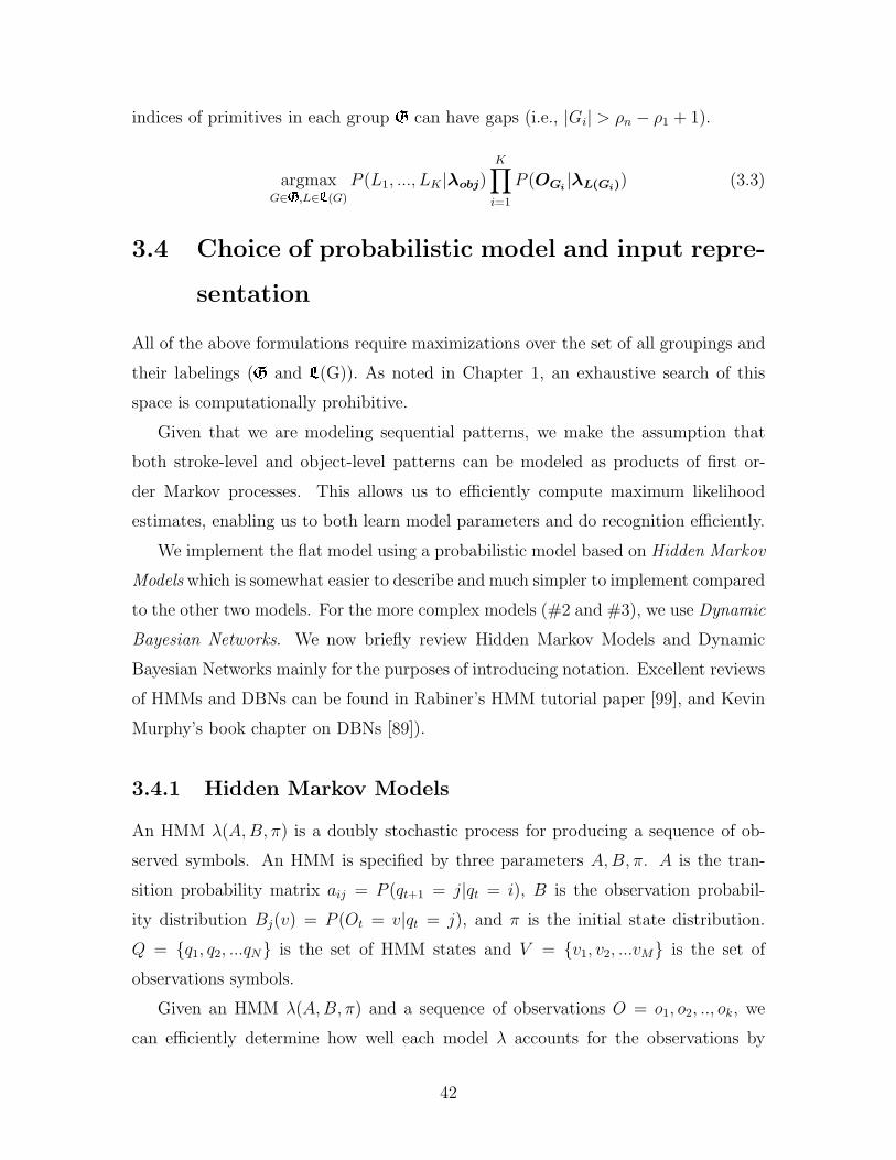
3.4 Choice of probabilistic model and input representation . . . . . . . . 42

3.4.1 Hidden Markov Models . . . . . . . . . . . . . . . . . . . . . . 42

3.4.2 Dynamic Bayesian Networks . . . . . . . . . . . . . . . . . . . 43

3.4.3 The input . . . . . . . . . . . . . . . . . . . . . . . . . . . . . 43

3.5 Flat model . . . . . . . . . . . . . . . . . . . . . . . . . . . . . . . . . 43

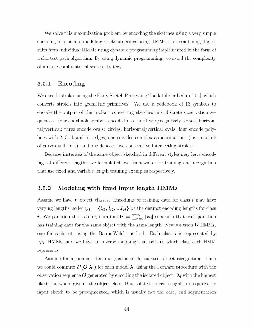
3.5.1 Encoding . . . . . . . . . . . . . . . . . . . . . . . . . . . . . 44

3.5.2 Modeling with fixed input length HMMs . . . . . . . . . . . . 44

3.5.3 Modeling using HMMs with variable length training data . . . 48

3.5.4 Advantages of the graph based approach . . . . . . . . . . . . 49

3.6 Multiscale model . . . . . . . . . . . . . . . . . . . . . . . . . . . . . 49

3.6.1 Encoding . . . . . . . . . . . . . . . . . . . . . . . . . . . . . 50

3.6.2 Model description . . . . . . . . . . . . . . . . . . . . . . . . . 50

3.6.3 Implementation issues . . . . . . . . . . . . . . . . . . . . . . 53

3.7 Multiscale-interspersing model . . . . . . . . . . . . . . . . . . . . . . 54

3.7.1 Switching parents . . . . . . . . . . . . . . . . . . . . . . . . . 56

3.7.2 Description of the model topology . . . . . . . . . . . . . . . . 57

3.8 Discussion . . . . . . . . . . . . . . . . . . . . . . . . . . . . . . . . . 61

4 Results 62

4.1 Circuit data collection . . . . . . . . . . . . . . . . . . . . . . . . . . 62

4.2 Generating an observation sequence . . . . . . . . . . . . . . . . . . . 63

4.3 Modeling object level patterns increases recognition accuracy . . . . . 64

4.3.1 Experiment setup and quantitative results . . . . . . . . . . . 64

4.3.2 Qualitative examples and discussion . . . . . . . . . . . . . . . 65

4.4 Handling interspersings increases recognition accuracy . . . . . . . . . 66

4.4.1 Experiment setup and quantitative results . . . . . . . . . . . 66

4.4.2 Quantifying errors per-interspersing . . . . . . . . . . . . . . . 69

4.4.3 Qualitative examples and discussion . . . . . . . . . . . . . . . 70

4.5 Summary . . . . . . . . . . . . . . . . . . . . . . . . . . . . . . . . . 74

10

5 Related work 75

5.1 Recognition systems . . . . . . . . . . . . . . . . . . . . . . . . . . . 76

5.1.1 Speech and handwriting recognition . . . . . . . . . . . . . . . 76

5.1.2 Graphics recognition . . . . . . . . . . . . . . . . . . . . . . . 77

5.1.3 Object recognition . . . . . . . . . . . . . . . . . . . . . . . . 77

5.1.4 Symbol recognition systems . . . . . . . . . . . . . . . . . . . 79

5.2 Pen-based interfaces . . . . . . . . . . . . . . . . . . . . . . . . . . . 80

5.2.1 Early processing systems . . . . . . . . . . . . . . . . . . . . . 80

5.2.2 Computer graphics and user interface applications . . . . . . . 80

5.3 Sketch recognition systems . . . . . . . . . . . . . . . . . . . . . . . . 81

5.3.1 Use of spatial data for recognition . . . . . . . . . . . . . . . . 81

5.3.2 Use of temporal data for recognition . . . . . . . . . . . . . . 84

6 Contributions 85

6.1 Contributions . . . . . . . . . . . . . . . . . . . . . . . . . . . . . . . 85

6.2 Discussion . . . . . . . . . . . . . . . . . . . . . . . . . . . . . . . . . 86

7 Future work 89

7.1 Alternative models of interspersing . . . . . . . . . . . . . . . . . . . 89

7.2 Incorporating other knowledge sources . . . . . . . . . . . . . . . . . 91

7.2.1 Incorporating user feedback . . . . . . . . . . . . . . . . . . . 91

7.2.2 Incorporating information from external classifiers . . . . . . . 91

7.3 Incorporating spatial features . . . . . . . . . . . . . . . . . . . . . . 93

7.4 User interface issues . . . . . . . . . . . . . . . . . . . . . . . . . . . 94

A Recognition results for non-color printing 95

B Symbols used 100

11

List of Figures

1-1 Examples of applications that use and manipulate graphical represen-

tations of objects. We believe such applications will benefit most from

sketch based interfaces. . . . . . . . . . . . . . . . . . . . . . . . . . . 19

1-2 In most design software, toolbars serve as the primary means of enter-

ing graphical information. Here we see toolbars that are part of the

user interface for the applications shown in Fig. 1-2. . . . . . . . . . 20

1-3 The goal of sketch recognition is to enable people to convey graphical

information by drawing. Imagine if an electrical engineer could draw

(a) and have the computer automatically construct the PSpice model

in (b). . . . . . . . . . . . . . . . . . . . . . . . . . . . . . . . . . . . 20

1-4 A circuit digram illustrating what we mean by a sketch. Our goal

is to group strokes forming the same object together (segmentation)

and determine what object they form (classification). In this case

segmentation finds the circled grouping and classification indicates that

they represent an NPN transistor. . . . . . . . . . . . . . . . . . . . . 21

1-5 Gesture based Graffiti input scheme for PDAs. Input gestures must

be drawn in a single stroke, starting at the heavy dot. Shapes of the

some gestures do not look like the intended symbols (e.g., ’%’, ’@’). . 23

1-6 Circuit diagram for an amplifier. Stroke ordering for a fragment of the

circuit is indicated by numbers. . . . . . . . . . . . . . . . . . . . . . 25

12

1-7 In this example, the user interspersed a wire connected to the collector

of the transistor Q2. We present a model that can recognize objects

correctly even in the presence of such interspersings and identify in-

terspersed objects (indicated by coloring the interspersed wire in black

instead of cyan). See Fig. A-1 for B&W printing. . . . . . . . . . . . 25

2-1 Example showing what we mean by a sketch. Note the messy, freehand

nature of the diagram. . . . . . . . . . . . . . . . . . . . . . . . . . . 29

2-2 Police sketches (left) and artistic renderings. Recognition of such

sketches fall outside the scope of this thesis. The police sketches were

taken from [112] which describes a system for face sketch recognition.

The baby and the womb drawing is by Leonardo da Vinci. . . . . . . . 30

2-3 Results of the “grape clusters” experiment by van Sommers [119].

Users were asked to copy each cluster on paper. Numbers in each

region show the average order in which the boundary was drawn and

shows the strong effects of planning and anchoring. . . . . . . . . . . 31

2-4 Examples of the figures that the users were asked to draw in the user

study. . . . . . . . . . . . . . . . . . . . . . . . . . . . . . . . . . . . 33

2-5 A sketching style diagram showing two ways of drawing stick-figures . 34

3-1 Symbols for stop and skip-audio-track (on the left), and a sketched stop

symbol (right). . . . . . . . . . . . . . . . . . . . . . . . . . . . . . . 36

3-2 An example showing a multi-object stroke. The selected circuit frag-

ment contains two wires and a resistor drawn using a single stroke. . 40

3-3 Training examples for the simple recognition problem that we will use

to illustrate our HMM based recognition method. We have two classes

(square and triangle). For simplicity assume the squares are drawn

using three or four strokes, and the triangles are drawn using two or

three strokes (i.e., ψsquare = {3, 4} and ψtriangle = {2, 3}). . . . . . . . 46

3-4 A simple scene consisting of a square and a triangle. Numbers indicate

the stroke ordering. . . . . . . . . . . . . . . . . . . . . . . . . . . . . 46

3-5 An illustration of graph construction for the sketch in Fig. 3-4 using

HMMs with fixed input length. . . . . . . . . . . . . . . . . . . . . . 47

13

3-6 The dynamic Bayesian network representing the model for capturing

stroke-level patterns. This fragment has a dual representation as a

hidden Markov model with continuous observations and M mixtures. 51

3-7 The dynamic Bayesian network representing the multiscale model. . . 52

3-8 An example of interspersing: The user draws two other objects (wires

#3 and #6) over the course of drawing the transistor. The drawing

order is indicated by numbers. . . . . . . . . . . . . . . . . . . . . . . 54

3-9 The dynamic Bayesian network representing our model that uses mul-

tiscale patterns and handles interspersed drawing. . . . . . . . . . . . 55

3-10 Example illustrating the switching parent mechanism. . . . . . . . . . 57

4-1 Examples of collected circuits. . . . . . . . . . . . . . . . . . . . . . . 63

4-2 Conversion to the primitive sequence. . . . . . . . . . . . . . . . . . . 64

4-3 One of the circuits drawn by our study participants. Stroke ordering

for a fragment of the circuit is indicated by numbers. . . . . . . . . . 67

4-4 Examples of errors corrected using context provided by object-level

patterns. There are four misrecognitions in (a). Note how two of these

misrecognitions is fixed using knowledge of object level patterns (resis-

tor in the upper left corner (R1) and the wire connected to the emitter

of the misrecognized transistor). See Fig. A-2 for B&W printing. . . 68

4-5 The dynamic Bayesian network representing the multiscale-interspersing

model that handles interspersed drawing. . . . . . . . . . . . . . . . . 69

4-6 Another circuit drawn by our study participants. Stroke ordering for

a fragment of the circuit is indicated by numbers. . . . . . . . . . . . 71

4-7 In this example, the user interspersed a wire connected to the collector

of the transistor on the right. As a result the transistor is misclassified

by the multiscale model (a). The multiscale-interspersing model identi-

fies the wire interspersing (indicated by black) and correctly interprets

the transistor (b). See Fig. A-3 for B&W printing. . . . . . . . . . . 72

14

4-8 Another example of handling interspersing. In this case the errors

caused by the interspersing is minor compared to 4-7. The inter-

spersed wire is interpreted to be part of the transistor. The multiscale-

interspersing model identifies the wire interspersing (indicated by black

in b). See Fig. A-4 for B&W printing. . . . . . . . . . . . . . . . . . 73

5-1 An example illustrating the kinds of input that graphics recognition

systems accept. Here is a typical input for the graphics recognition

system described in [82] and the processing of the system. . . . . . . 77

6-1 An example of strokes with the right temporal character but wrong

shape being classified incorrectly (reproduced from Chap. 4). The two

vertical lines (l1, l2) are offset from one another, but were classified to

be a capacitor because they were drawn one after the other, and the

temporal features extracted from them agree with the capacitor model

that we learned. See Fig. A-5 for B&W printing. . . . . . . . . . . . . 87

7-1 One plausible way of modeling self interspersing could be to duplicate

the stroke level model for the self interspersing class. . . . . . . . . . 90

7-2 Suppose the user drew the above circuit diagram and the recognition

system misclassified the circled capacitor. Now, if the user selects these

two strokes and labels them explicitly as forming a capacitor, then we

can take this information as being ground truth. This allows us to

inject this information directly into our DBN model by making certain

nodes in the unrolled DBN observed (see Fig. 7-3). . . . . . . . . . . 92

7-3 If the user explicitly corrects a misrecognition as describe in Fig. 7-2,

then this makes certain nodes in the unrolled DBN observable (nodes

circled with dashed lines). When we perform inference with the new

observed values, the effects of the observations will propagate to the

neighboring nodes (nodes circled with dotted lines). . . . . . . . . . . 92

15

7-4 One way of incorporating information from external classifiers would

be to use the provided information as soft evidence [118] or virtual ev-

idence [101] by having a child node associated with each MUX node as

shown here. The EC node carries information supplied by the external

classifiers. . . . . . . . . . . . . . . . . . . . . . . . . . . . . . . . . . 93

A-1 In this example, the user interspersed a wire connected to the collector

of the transistor Q2. We present a model that can recognize objects

correctly even in the presence of such interspersings and identify inter-

spersed objects (indicated by I-W). . . . . . . . . . . . . . . . . . . . 95

A-2 Examples of errors corrected using context provided by object-level

patterns. There are four misrecognitions in (a). Note how two of

these misrecognitions is fixed using knowledge of object level patterns

(resistor in the upper left corner (R1) and the wire connected to the

emitter of the misrecognized transistor). . . . . . . . . . . . . . . . . 96

A-3 In this example, the user interspersed a wire connected to the collector

of the transistor on the right. As a result the transistor is misclassified

by the multiscale model (a). The multiscale-interspersing model iden-

tifies the wire interspersing (indicated by I-W) and correctly interprets

the transistor (b). . . . . . . . . . . . . . . . . . . . . . . . . . . . . . 97

A-4 Another example of handling interspersing. In this case the errors

caused by the interspersing is minor compared to 4-7. The inter-

spersed wire is interpreted to be part of the transistor. The multiscale-

interspersing model identifies the wire interspersing (indicated by I-W

in b). . . . . . . . . . . . . . . . . . . . . . . . . . . . . . . . . . . . 98

A-5 An example of strokes with the right temporal character but wrong

shape being classified incorrectly (reproduced from Chap. 4). The two

vertical lines (l1, l2) are offset from one another, but were classified to

be a capacitor because they were drawn one after the other, and the

temporal features extracted from them agree with the capacitor model

that we learned. . . . . . . . . . . . . . . . . . . . . . . . . . . . . . . 99

16

List of Tables

2.1 A summary of the statistics from our user study for a subset of the

symbols drawn by the users (shown in Fig.2-4). Note that 120=5!,

720=6! and 40320=8!. Users drew 30 or more examples of each object. 33

4.1 Mean correct recognition rates for the baseline system (μb) and the

multiscale model (μm) on sketches collected from 8 participants. The

table also shows the percentage reductions in the error rates and max-

imum error reductions achieved for each user as percentages (Δerr and

maxΔ). On average, modeling object-level patterns always improves

performance. . . . . . . . . . . . . . . . . . . . . . . . . . . . . . . . 66

4.2 Mean correct recognition rates for the multiscale-interspersing (μm−i)

and the multiscale models (μm) for users who exhibited interspersed

drawing behavior. The table also shows the percentage reductions in

the error rates and maximum error reductions achieved for each user

as percentages (Δerr and maxΔ). On average, handling interspersing

patterns always improves performance. . . . . . . . . . . . . . . . . . 67

4.3 This table shows the number of misrecognized primitives per inter-

spersing. The first two row shows the number of total primitives in

each sketch and the number of added interspersings. Next two rows

show the number of primitives incorrectly recognized by the baseline

and by our model. The next row shows the number of primitives that

the baseline misses because it cannot handle interspersings and the last

row is the number of primitives missed by the baseline per interspersing. 70

17

Chapter 1

Introduction

1.1 Why do sketch recognition?

Sketching is a natural modality of communication employed in a wide variety of

settings. People sketch during early design and brainstorming sessions to guide the

thought process and use sketches as a means of documentation[117]. We use sketching

to convey thoughts that can not be put in words.

The increasing availability of pen based hardware such as PDAs and Tablet PCs

makes capturing sketches easier than ever. Despite their ubiquity, suitability for

certain HCI tasks, and the availability of supporting hardware, there is little computer

support for sketching.

We believe making computers “sketch literate” will produce smarter, more natural

user interfaces for a host of computer applications. Applications to benefit most from

sketch based interfaces are the ones that use and manipulate graphical representations

of objects. Fig. 1-1 shows examples of such commercial applications: a 2D rigid body

physics simulator (Fig. 1-1.a), an analog circuit simulator (Fig. 1-1.b), a UML design

tool (Fig. 1-1.c), and PowerPoint (Fig. 1-1.d).

All of these applications currently share the same user interface paradigm based

on mouse and keyboard input. Toolbars of the sort shown in Fig. 1-2 serve as the

primary means of entering graphical information. In most cases, changing the de-

fault parameters of the graphical objects requires further keyboard and mouse input

through menus and dialog boxes.

18

(a) Working Model 2D (b) PSpice

(c) UMLStudio (d) PowerPoint

Figure 1-1: Examples of applications that use and manipulate graphical representa-tions of objects. We believe such applications will benefit most from sketch basedinterfaces.

Our goal in building sketch recognition systems is to allow people to convey graphi-

cal information in the same way that they have done for thousands of years: simply by

drawing. Imagine, for example, if an electrical engineer could draw the freehand cir-

cuit diagram in Fig. 1-3.a and have the computer automatically construct the PSpice

model in Fig. 1-3.b. This is what we mean by sketch recognition and in this thesis,

we show how it can be done by extracting as much information as it is practically

possible from temporal patterns that appear during sketching.

19

Figure 1-2: In most design software, toolbars serve as the primary means of enteringgraphical information. Here we see toolbars that are part of the user interface for theapplications shown in Fig. 1-2.

(a) A freehand circuit diagram. (b) What we wish to obtain from (a).

Figure 1-3: The goal of sketch recognition is to enable people to convey graphicalinformation by drawing. Imagine if an electrical engineer could draw (a) and havethe computer automatically construct the PSpice model in (b).

20

Figure 1-4: A circuit digram illustrating what we mean by a sketch. Our goal is togroup strokes forming the same object together (segmentation) and determine whatobject they form (classification). In this case segmentation finds the circled groupingand classification indicates that they represent an NPN transistor.

1.2 What is sketch recognition?

The basic task of sketch recognition can be understood best by considering the input

and the output.

By a sketch, we mean messy, informal hand-done drawings (e.g., Fig. 1-4). Specif-

ically we are interested in recognizing sketches with objects of a symbolic nature that

can be represented using structural descriptions, which have been the focus of the

sketch recognition community [4, 107, 84, 45, 30].

It is worth emphasizing that we are interested in sketches that are drawn naturally

as the user would draw on a piece of paper. This is unlike some systems that require

users to draw each object using a single stroke, or pause after drawing each object to

facilitate segmentation, thereby reducing the problem of sketch recognition to that of

isolated symbol recognition.

We specifically refrain from forcing the user to sketch in a certain way or follow

certain conventions during sketching. Consequently, our recognition algorithms will

21

have to deal with unsegmented sketches with multi-stroke objects and drawing with

interspersed objects (i.e., starting a new object before completing the current one).

Earlier we gave an informal definition of sketch recognition as the process of au-

tomatically converting freehand input into a representation which can be used by

domain specific applications. A more formal definition of sketch recognition can be

characterized in terms of three tasks:

• Segmentation: The task of grouping strokes so that those constituting the

same object end up in the same group. At this point it is not known what object

the strokes form. For example, in Fig. 1-4, the correct segmentation gives us

fifteen disjoint sets of strokes (assuming each wire segment is a single object).

• Classification: Classification is the task of determining which object each

group of strokes represents. For Fig. 1-4, recognition would indicate that the

circled strokes represent an NPN transistor.

• Labeling: Labeling is the task of assigning labels to components of a recog-

nized object (e.g., identifying the terminal with the current symbol in the NPN

transistor in Fig. 1-4 as the emitter terminal).

Although the three tasks described above are conceptually separate, in any real

sketch recognition scenario they may be intermixed. For example, it could be the case

that a particular recognition architecture classifies objects and labels their constituent

parts simultaneously. More likely, segmentation is done first, followed by classification

and labeling.

1.3 Sketching is more than Graffiti

Graffiti is a single stroke gesture recognition scheme developed mainly for PDAs. One

of the most popular gesture recognition methods for Graffiti-like input is described

by Rubine [102]. Fig. 1-5 shows the Graffiti alphabet for punctuation and various

symbols.

True sketch recognition is a different and much more challenging problem than

recognizing the carefully prescribed strokes used in Graffiti. Unlike freehand drawing,

22

Figure 1-5: Gesture based Graffiti input scheme for PDAs. Input gestures must bedrawn in a single stroke, starting at the heavy dot. Shapes of the some gestures donot look like the intended symbols (e.g., ’%’, ’@’).

the Graffiti alphabet comes with a number of conventions and restrictions that make

it easy to recognize but unnatural. In particular:

• Symbols are specified by gestures that do not necessarily resemble the target

shapes (e.g. ’%’, ’@’ in Fig. 1-5).

• Input gestures must be drawn in a single stroke.

• The gesture must start at a predetermined point (the heavy dots shown in

Fig. 1-5).

• The starting point may affect classification because some symbols are specified

with the same gesture but different starting points (e.g., [ and { in Fig. 1-5).

These restrictions conflict with our goal of supporting freehand drawing where

users can sketch without worrying about adhering to certain drawing guidelines.

1.4 Combinatorics makes sketch recognition hard

Treating sketches as images leads to recognition algorithms with exponential time

complexities [84]: subgraph isomorphism-based methods and correspondence-based

approaches have exponential time complexities. If we assume that we have m object

classes and that each object model has k components, a simple calculation shows that

23

in the worst case, recognizing an object surface with n strokes requires(

nk

)grouping

operations and k! constraint checking operations, yielding a total of m(

nk

)k! opera-

tions. In practice, the combinatorics get even worse because sketches are inherently

noisy (e.g. due to digitization) and messy (e.g. sloppy drawing by the user).

Exponential time and space requirements are unacceptable for interactive sketch

recognition, because giving users feedback about the recognition results is an essential

part of sketch based interfaces[4]. Sketch recognition algorithms proposed so far

either don’t run in real-time [4], or make limiting assumptions about the domains

(e.g., maximum object size, maximum number of strokes per object [108, 83, 85]).

Furthermore most of these approaches have been demonstrated only in domains where

objects are non-touching and hence segmentation is less of an issue compared to

more challenging domains where objects may overlap or touch one another (e.g.,

box-connector type diagrams such as UML diagrams, family trees, circuit diagrams).

1.5 Using temporal patterns allows efficient sketch

recognition

This thesis describes an approach to efficient sketch recognition. We show how treat-

ing sketching as an incremental and interactive process enables polynomial time recog-

nition algorithms, by allowing us to exploit naturally appearing temporal patterns in

sketching.

Current sketching systems are indifferent to who is using the system, employing

the same recognition routines for all users. But user studies we have conducted

indicate clearly that different users have different sketching preferences and styles,

and that there is considerable value in being able to capture these different styles.

A major component of individual drawing styles is the temporal patterns seen

during sketching. For example, when people draw stick figures, one frequently seen

stroke-level pattern is a sequence consisting of a circular stroke, followed by a vertical

line, followed by two pairs of positively and negatively sloped lines – respectively

corresponding to the head, body, arms and legs of the stick-figure. It is these kinds

of temporal patterns that can aid sketch recognition. Using temporal patterns allows

24

Figure 1-6: Circuit diagram for an amplifier. Stroke ordering for a fragment of thecircuit is indicated by numbers.

us to work with one dimensional time series data, for which there are efficient, sound

mathematical analysis methods.

Consider the circuit diagram in Fig. 1-6, showing an amplifier circuit and the stroke

ordering for a fragment of the circuit of particular interest to us. Using the hierarchical

probabilistic models that we present in this thesis, we can learn multiscale temporal

patterns that naturally exist in the creation of such a sketch and interpret it under a

second on a standard PC. Our hierarchical models capture knowledge of both common

stroke orderings and common object orderings. Results of our evaluation involving

circuit diagrams collected from eight participants show that modeling common object

orderings reduces the number of recognition errors by 14%- 37%.

Furthermore our temporal model explicitly models interspersed drawing behavior

and does not require the users to draw one object at a time. This means we can rec-

ognize sketches correctly even if the user starts drawing a new object before finishing

the current one. For example, we can correctly recognize the circuit in Fig. 1-6 even

though a wire (part of stroke #15) was drawn in the course of drawing the transis-

tor Q2. Fig. 1-7 shows the interpretation of our system. Such interspersed drawing

behavior poses serious challenges to a naıve temporal model for sketch recognition,

25

100 200 300 400 500 600 700 800 900

−100

0

100

200

300

400

500

result npn resistor capacitor battery wire interspersing

Figure 1-7: In this example, the user interspersed a wire connected to the collectorof the transistor Q2. We present a model that can recognize objects correctly evenin the presence of such interspersings and identify interspersed objects (indicatedby coloring the interspersed wire in black instead of cyan). See Fig. A-1 for B&Wprinting.

but we show how the issue can be addressed remaining within the formal frame-

work of Dynamic Bayesian Networks. We show that modeling interspersing reduces

recognition errors by an additional 20%-37%.

Finally our recognition framework supports multi-object strokes (e.g., stroke #15

in Fig. 1-6 represents a wire and part of the transistor Q2), multi-stroke objects

(e.g., Q1 consists of four strokes), objects with a variable number of components

(e.g., some resistors have fewer humps). We also support discrete and real-valued

feature representations which allows us to encode our data using discrete encodings

for categorical properties (e.g., a stroke being a circle vs. a line), and real-valued

encodings for continuous features (e.g., length, orientation of a line). We report that

a numerically stable belief propagation algorithm known as the Lauritzen-Jensen

stable conditional Gaussian belief propagation algorithm should be used for modeling

discrete and real-valued features.

26

1.6 Thesis roadmap

The next chapter summarizes properties of sketches and reports results from a user

study that we conducted to measure the degree to which people use predictable stroke

orderings when they sketch. Chapter three gives a formal description of the sketch

recognition problem and introduces our model that uses hierarchical graphical mod-

els to model multiscale patterns in sketching while supporting interspersed drawing.

Chapter three also introduces two baseline methods that we use in our evaluation. In

chapter four, we report evaluation results comparing the performance of our model

to the two baseline models. Chapters five and six summarize the related work and

our main contributions. We conclude with future work.

27

Chapter 2

Properties of sketches

Here we briefly summarize properties of sketches because it is important to understand

the nature of the data that we are dealing with.

2.1 Static properties of sketches

The static properties of sketches are those that would be present even if all we had was

a scanned image of the sketch. They include image-like properties such as digitization

noise and others that are specific to sketches, such as messiness.

Noise arises from digitization performed by a digitizing tablet, a scanner, or an-

other imaging device. Each device has an inherent resolution and noise characteristics.

Messiness refers to phenomena such as overshooting, undershooting, messiness in

the lines and jitters due to hand tremor. For example, in Fig. 2-1, stroke segments

making the humps of the resistors don’t always make the same angle, and some humps

are relatively shorter although in an ideal resistor symbol, each segment is perfectly

linear and they make the same angle. The missing connection between the capacitor

in Fig. 2-1 and the wire above it is an example of undershooting – another kind

of messiness. It is these kinds of phenomena resulting from the kinesthetic nature

of sketching that makes sketch recognition a much harder problem than diagram

recognition studied extensively by the document analysis community [114, 11].

Sketches are highly informal. Instances of the same icon may have varying aspect

ratios and scales. Parts (subcomponents) of an object may have varying aspect ratios

28

Figure 2-1: Example showing what we mean by a sketch. Note the messy, freehandnature of the diagram.

within the object. This high variability rules out popular transformation space search

approaches that rely on affine properties of images.

The sketches we deal with are mostly iconic (e.g., a “light bulb” representing an

idea, or a stick-figure representing a person). Their iconic nature makes it possible to

have symbolic descriptions of sketches. There are also domains with highly non-iconic

properties, such as “police sketches” or artistic renderings which fall outside the scope

of this thesis (Fig. 2-2).

Most sketches can be broken down into compositions of simpler objects, and those

objects can be further broken down into primitives such as lines, circles etc. For

example, a simple sketch of a car can be broken down into the body, and the wheels;

and the wheels can be further broken down into two circles representing the wheel

and the axle.

2.2 Dynamic properties of sketches

One of the advantages of online sketching is that a sketch can be captured as it is

constructed, making it possible to capture properties that may potentially aid recog-

nition. Our stroke-based representation allows us to access stroke level information

29

Figure 2-2: Police sketches (left) and artistic renderings. Recognition of such sketchesfall outside the scope of this thesis. The police sketches were taken from [112] whichdescribes a system for face sketch recognition. The baby and the womb drawing is byLeonardo da Vinci.

including what order the strokes came in, as well as timing information for individual

points.

Because sketching is incremental (i.e, strokes are put on the sketching surface one

at a time) the sketching surface will at almost every moment have on it a partially

drawn object. Partially drawn objects are a common source of ambiguity in sketches.

They can act as spurious strokes and confuse recognition algorithms. Partially drawn

objects also raise the difficult issue of balancing the desire to generate all plausible

recognition hypotheses and the desire to wait until there are enough components so

the search is more constrained. The methods that we present explicitly address these

issues by modeling the sketching process using a set of variables that, among other

things, capture our belief about whether the user has done drawing the current object.

In a typical sketch recognition scenario, there is two way communication: infor-

mation flows from the user to the computer via the strokes drawn and the editing

operations, and from the computer to the user via computer’s display of its interpre-

tation of the strokes and editing operations. This interactive nature of sketching is

an important source of knowledge when it comes to confirming the correctness of a

30

Figure 2-3: Results of the “grape clusters” experiment by van Sommers [119]. Userswere asked to copy each cluster on paper. Numbers in each region show the averageorder in which the boundary was drawn and shows the strong effects of planning andanchoring.

system’s interpretation. For example, the longer the user lets an interpretation exist,

the more certain the system can be about its interpretation [6]. It is therefore impor-

tant to have recognition algorithms that are fast enough to provide realtime feedback

to the user.

Sketching is highly stylized in the sense that people have strong biases in the way

they sketch (e.g., people draw enclosing objects first, use a left-to-right stroke ordering

when drawing symmetric objects). There is psychological evidence attributing such

phenomena to motor convenience, part saliency, hierarchy, geometric constraints,

planning and anchoring [116, 119]. For example, Fig. 2-3 shows the results of the

“grape clusters” experiment described by van Sommers [119] where the users were

asked to copy four clusters on paper. Numbers in each region show the average

order in which the boundary was drawn and shows the strong effects of planning and

anchoring.

31

Existence of ordering patterns during drawing is significant from a recognition

perspective because the regularities in sketching can be used for recognition. Because

this forms the basis for our approach to recognition presented chapter 3, and we

conducted user studies to validate this observation for domains of interest to us.

2.3 Temporal patterns appear to be common in

sketching

We ran a user study to assess the degree to which people have sketching styles, i.e.,

a reasonably consistent stoke order used when drawing an item. For example, if one

starts drawing a stick-figure with the head, then draws the torso, the legs and the

arms respectively, we regard this as a style different from the one where the arms are

drawn before the legs (see Fig. 2-5).

Our user study asked users to sketch various icons, diagrams and scenes from six

domains. Example tasks included drawing:

• Finite state machines performing simple tasks such as recognizing a regular

language.

• Unified Modeling Language (UML) diagrams depicting the design of simple

object-oriented programs.

• Scenes with stick-figures playing certain sports.

• Course of Action Diagram symbols used in the military to mark maps and plans.

• Digital circuit diagrams that implement a simple logic expression.

• Emoticons expressing happy, sad, surprised and angry faces.

We asked 10 subjects to sketch three sketches from each of the six domains,

collecting a total of 180 sketches. Requests were given to subjects in an arbitrary

order to intersperse domains and reduce the correlation between sketching styles

used in different instances of sketches from the same domain. Sketches were captured

using a digitizing LCD tablet.

32

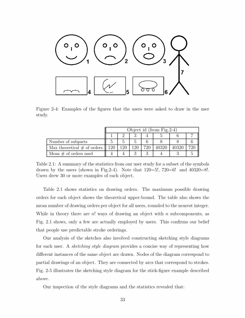
Figure 2-4: Examples of the figures that the users were asked to draw in the userstudy.

Object id (from Fig.2-4)1 2 3 4 5 6 7

Number of subparts 5 5 5 6 8 8 6Max theoretical # of orders 120 120 120 720 40320 40320 720Mean # of orders used 4 4 3 3 4 3 5

Table 2.1: A summary of the statistics from our user study for a subset of the symbolsdrawn by the users (shown in Fig.2-4). Note that 120=5!, 720=6! and 40320=8!.Users drew 30 or more examples of each object.

Table 2.1 shows statistics on drawing orders. The maximum possible drawing

orders for each object shows the theoretical upper-bound. The table also shows the

mean number of drawing orders per object for all users, rounded to the nearest integer.

While in theory there are n! ways of drawing an object with n subcomponents, as

Fig. 2.1 shows, only a few are actually employed by users. This confirms our belief

that people use predictable stroke orderings.

Our analysis of the sketches also involved constructing sketching style diagrams

for each user. A sketching style diagram provides a concise way of representing how

different instances of the same object are drawn. Nodes of the diagram correspond to

partial drawings of an object. They are connected by arcs that correspond to strokes.

Fig. 2-5 illustrates the sketching style diagram for the stick-figure example described

above.

Our inspection of the style diagrams and the statistics revealed that:

33

Figure 2-5: A sketching style diagram showing two ways of drawing stick-figures

• People sketch objects in a highly stylized fashion. In drawing the stick figure,

for example, one of our subjects always started with the head and the torso,

and finished with the arms or the legs (Fig.2-5).

• Individual sketching styles persist across sketches.

• Subjects prefer an order (e.g., left-to-right) when drawing symmetric objects

(e.g., the two arms) or arrays of similar objects (e.g., three collinear circles).

• Enclosing shapes are usually drawn first (e.g., the outer circle in emoticons, or

the enclosing rectangles in Fig. 2-4).

The user study confirmed our conjecture about the stylized nature of sketching

in a number of domains that have received the attention of the sketch recognition

community. In order to capitalize on this, we constructed a probabilistic model for

learning temporal patterns in sketching and use them for sketch recognition.

34

Chapter 3

Approach

This chapter describes our approach to sketch recognition. Our model is designed to

take advantage of the rich temporal patterns that exist in sketching while supporting

interspersed drawing. To facilitate the explanation of this model and to serve as

baseline systems, we also introduce two simpler models.

We start by discussing a toy example to illustrate the intuition behind using stroke

ordering information for sketch recognition. We then describe properties that we want

our models to have and give formal definitions of the terms we will use in the rest of

this chapter.

3.1 The intuition

To make the basic intuition clear, we start with an over-simplified task scenario.

Assume we have only two symbols to recognize: skip-audio-track and stop, and assume

the user always draws them using the same stroke ordering, indicated by the numbers

in Fig. 3-1-a. Finally, assume we need to recognize which of these symbols is present

in a scene known to contain only a single instance of one of them (i.e., isolated object

recognition).

Suppose the user draws the stop symbol as shown in Fig. 3-1-b. Assuming we can

reliably recognize the individual strokes as lines and tell whether they are horizontal

(H), vertical (V), negatively/positively sloped (N, P), we can look at the order in

which the user drew the lines and classify the input as a stop symbol if we see the

35

(a) (b)

Figure 3-1: Symbols for stop and skip-audio-track (on the left), and a sketched stopsymbol (right).

[V, H, V, H] ordering, and as a skip-track symbol for the [V, P, N, V] ordering.

The above approach works by encoding the user input to generate an observation

sequence describing the scene (e.g. [V, H, V, H]), and comparing this sequence to

its model of how the user is known to sketch. The result of the comparison is binary,

indicating whether we have a match. This toy example shows how stroke ordering

can be used for recognition in an over-simplified scenario.

3.2 Desired features of a model

We see the following properties as being important for models of sketch recognition.

3.2.1 Handling stroke-level patterns

As noted in chapter 2, stroke orderings used in the course of drawing individual objects

naturally contain certain patterns. We call these stroke-level patterns because they

capture the probability of seeing a sequence of strokes with certain properties when

sketching a particular object. We want our sketch recognition algorithms to capture

these patterns.

3.2.2 Support for multiple classes and drawing orders

We should be able to recognize multiple classes of objects. We also want to accommo-

date multiple drawing orders instead of just one. For example, it may be the case that

sometimes the user sketches the stop symbol starting with a horizontal line. Further-

36

more, if the user prefers one drawing order more frequently than others, this should

be accounted for as well. This requires using training and classification methods that

can use such information.

3.2.3 Handling variations in encoding length

Users should be able to draw freely. For example, they should be able to draw the

stop symbol using three strokes instead of four, or draw a resistor with five humps

instead of six (thus generating an encoding of the input with only five observations

instead of six).

3.2.4 Probabilistic matching score

We would like the result of matching an observation sequence against a model to

be a continuous value reflecting the likelihood of using that particular drawing order

for drawing the object. This is required if we are to have a mathematically sound

framework for combining the outputs of multiple matching operations for scenes with

multiple objects such that, among plausible interpretations, those corresponding to

more frequently used orders are preferred.

3.2.5 Learning compact representations

In practice, different drawing orders will have similar subsequences. Ideally the system

should learn compact representations of drawing orders from labeled sketch examples.

3.2.6 Rich feature representation

One of the steps in applying machine learning techniques to a problem is to decide

on a set of features that are sufficiently expressive given the problem at hand. In

sketch recognition, we deal with data that is most naturally described using geometric

features such as the shape of a stroke segment, length and orientation of line segments,

radii of circles etc. Some of these features are categorical (e.g., shape of a stroke

segment can be arc, line etc.) and are best represented using discrete variables.

Other features such as length and orientation are real-valued quantities and should

37

be represented as such. Therefore our algorithms should be able to represent both

discrete and real-valued features.

3.2.7 Handling object-level patterns

Another kind of temporal pattern present in online sketches is an object-level pat-

tern that captures the probability of seeing a certain sequence of objects being drawn.

Consider the domain of UML class diagrams drawn by software designers to describe

inheritance relationships, generalizations, associations, etc. In this domain, when a

designer draws a new class (indicated by a rectangle), it is natural to expect that the

new object will be connected with an arrow to one or more of the objects drawn ear-

lier. So in this domain, it is natural to have arrows drawn after a new class is created,

which we define as an object-level pattern. It is also natural to expect that the kind

of arrow will be different if the newly created class was a final class (because final

classes cannot be extended).

It is easy to imagine that this sort of domain specific knowledge about object-level

patterns could be a powerful addition to a UML diagram recognition system, and to

sketch recognition systems in general. But not every domain may have patterns

that are as well understood as they are for UML diagrams. And even if experts

could identify such patterns, incorporating them into a recognition system would

be a laborious task at best, considering all the ways in which various objects may

combine together. We argue that a better way of incorporating object-level temporal

patterns in a recognition framework would be to learn such features from data —

along with stroke-level patterns — and use them in recognition. Therefore the ability

to model object-level patterns is yet another feature we want.

3.2.8 Ability to handle interspersed drawing

During sketching, although people most often complete each object before starting

a new one, as we show later they sometimes draw other objects before completing

the current one. Such drawing behavior may severely hinder recognition unless the

recognition algorithms deal with it explicitly. The ability to handle interspersed

drawing is thus another feature that we desire.

38

3.3 Terminology and problem formulation

3.3.1 Terminology

We define a sketch S = S1, S2, ...SN as a sequence of strokes captured using a

digitizer, preserving the drawing order. 1 A stroke is defined as a set of time-ordered

points sampled between pen-down and pen-up events during sketching.

Each stroke is broken into several geometric primitives such as line and arc

segments as part of the preprocessing of the sketch, so let P = P1, P2, ...PT be the

sequence of time-ordered primitives obtained from S . Because the preprocessing of

a stroke may result in more than one primitive, the total number of primitives can

be larger than the number of strokes.

We use segmentation to refer to the task of grouping together primitives con-

stituting the same object. Given a set of classes C = {C1, C2, ...Cn} classification

refers to the task of determining which object each group of primitives represents (e.g.,

a stick-figure or a rectangle). Segmentation produces K groups G = G1, G2, ...GK ,

and classification gives us the labels for the groups L = L1, L2, ...LK , Li ∈ C . Each

group is defined by the indices of the primitives included in the group Gi = ρ1, ρ2, ...ρn

sorted in ascending order, so for cases where we don’t allow interspersing |Gi| =

ρn − ρ1 + 1.

We define sketch recognition as the segmentation and classification of a sketch.

A simplifying assumption in most sketch recognition systems is that a stroke can

be part of only one object. Our definition of segmentation in terms of primitive

groupings is more general than a definition based on stroke groupings and as long

as primitives are not shared across objects it allows a stroke to be part of multiple

objects (e.g., drawing a box and an arrow, or a resistors and a pair of wires in a single

stroke (Fig. 3-2)).

Finally we use the term observations to refer to the sequence of features O =

O1, O2, ..., OT obtained from the primitives. We use OGito refer to the sequence of

observations corresponding to a group of primitives Gi.

1We will use the Matlab notation begin : end as a shorthand for a list of indices that begins withstart and ends with end (i.e., 1:4 = 1 2 3 4). We will also use this notation in subscripts to denotea list of items (i.e., S1:N = S1, S2, ...SN ).

39

Figure 3-2: An example showing a multi-object stroke. The selected circuit fragmentcontains two wires and a resistor drawn using a single stroke.

3.3.2 Problem formulation

We consider three models. The first two serve as baseline methods in our evaluations

and help introduce our multiscale-interspersing model. Our model can learn both

object-level patterns and stroke-level patterns, and it explicitly models interspersed

drawing.

Model 1: Flat model

This model implements the first five features listed in section 3.2: It can learn compact

representations of stroke ordering patterns for multiple objects, each of which can be

drawn in more than one way, using a variable number of strokes.

Given a sequence of time-ordered primitives obtained from a sketch, the goal of

this model is to find a segmentation and classification of the primitives that maximizes

the likelihood of stroke-level patterns. Over all possible ways in which the primitives

can be grouped, �, and all possible ways in which these groups can be labeled,

�(G), we want the grouping G ∈ � and the labeling L ∈ �(G) that maximizes

the likelihood of the stroke-level observable features OGifor each group Gi given the

model corresponding to its label (λL(Gi)).

40

More formally, this can be written as a maximization problem, the solution to

which gives us the segmentation and labeling of the input sketch.

argmaxG∈�,L∈�(G)

K∏i=1

P (OGi|λL(Gi)) (3.1)

Model 2: Multiscale model

This model extends the flat model by adding the ability to have real-valued feature

vectors and the ability to handle object-level patterns in addition to stroke-level

patterns.

Given a sequence of time-ordered primitives obtained from a sketch, the goal of

this model is to find a segmentation and classification of the primitives such that

the likelihood of stroke-level patterns and object-level patterns is maximized simul-

taneously. Over all possible ways in which the primitives can be grouped, �, and

all possible ways in which these groups can be labeled, �(G), we want the grouping

G ∈ � and the labeling L ∈ �(G) that:

• maximizes the likelihood of the sequence of labels L1, L2, ..., LK given our model

for object-level patterns (λobj), and

• maximizes the likelihood of the stroke-level observable features OGifor each

group Gi given the stroke-level model corresponding to its label (λL(Gi)).

The terms corresponding to the stroke-level and object-level patterns can be writ-

ten together to obtain the following maximization problem, the solution to which

gives us the segmentation and labeling of the input sketch.


P (L1, ..., LK |λobj)

K∏i=1


The expression above is maximized over the set of all groupings and their labelings

(� and �(G)).

Model 3: Multiscale-interspersing model

This model adds the ability to handle interspersed drawing to the multiscale model.

The formulation of the recognition problem is the same as above, except now the

41

indices of primitives in each group � can have gaps (i.e., |Gi| > ρn − ρ1 + 1).


P (L1, ..., LK |λobj)K∏

i=1


3.4 Choice of probabilistic model and input repre-

sentation

All of the above formulations require maximizations over the set of all groupings and

their labelings (� and �(G)). As noted in Chapter 1, an exhaustive search of this

space is computationally prohibitive.

Given that we are modeling sequential patterns, we make the assumption that

both stroke-level and object-level patterns can be modeled as products of first or-

der Markov processes. This allows us to efficiently compute maximum likelihood

estimates, enabling us to both learn model parameters and do recognition efficiently.

We implement the flat model using a probabilistic model based on Hidden Markov

Models which is somewhat easier to describe and much simpler to implement compared

to the other two models. For the more complex models (#2 and #3), we use Dynamic

Bayesian Networks. We now briefly review Hidden Markov Models and Dynamic

Bayesian Networks mainly for the purposes of introducing notation. Excellent reviews

of HMMs and DBNs can be found in Rabiner’s HMM tutorial paper [99], and Kevin

Murphy’s book chapter on DBNs [89]).

3.4.1 Hidden Markov Models

An HMM λ(A, B, π) is a doubly stochastic process for producing a sequence of ob-

served symbols. An HMM is specified by three parameters A, B, π. A is the tran-

sition probability matrix aij = P (qt+1 = j|qt = i), B is the observation probabil-

ity distribution Bj(v) = P (Ot = v|qt = j), and π is the initial state distribution.

Q = {q1, q2, ...qN} is the set of HMM states and V = {v1, v2, ...vM} is the set of

observations symbols.

Given an HMM λ(A, B, π) and a sequence of observations O = o1, o2, .., ok, we

can efficiently determine how well each model λ accounts for the observations by

42

computing P (O|λ) using the Forward algorithm; compute the best sequence of HMM

state transitions for generating O using the Viterbi algorithm; and estimate HMM

parameters A, B and π to maximize P (O|λ) using the Baum-Welch algorithm.

3.4.2 Dynamic Bayesian Networks

Bayesian networks encode the joint probability of a set of variables Z = {Z1, ..., Zn}where the graphical structure of the network encodes the conditional dependencies

among the variables. DBNs are extensions of Bayesian networks that model joint

distribution of a set of variables over time by representing the conditional dependen-

cies between the variables using a pair of Bayesian networks (B1, B�). B1 defines the

prior for the Zi values at time t = 1, and B�

defines how variables at time t+1 relate

to each other and to those from time t.

HMMs are quite expressive as statistical models for time series [17, 16]. They are

also closely related to DBNs and it is possible to convert a DBN to an equivalent HMM

and vice versa. For the multiscale model and the interspersing multiscale model, we

choose to use a DBN representation because they allow parsimonious representations

of generative processes.

3.4.3 The input

The input to our models is the observation sequence O = O1:T obtained by com-

puting features from corresponding primitives P = P1:T . For the first model, we

use only discrete observations, while for the others we support both discrete and

real-valued (continuous) observations which allows us to have richer features while

avoiding discretization problems.

3.5 Flat model

As a reminder, the goal of this model is to segment and label an input sketch by

finding the solution to the expression in Eq. 3.1, reproduced below:


K∏i=1


43

We solve this maximization problem by encoding the sketches using a very simple

encoding scheme and modeling stroke orderings using HMMs, then combining the re-

sults from individual HMMs using dynamic programming implemented in the form of

a shortest path algorithm. By using dynamic programming, we avoid the complexity

of a naıve combinatorial search strategy.

3.5.1 Encoding

We encode strokes using the Early Sketch Processing Toolkit described in [105], which

converts strokes into geometric primitives. We use a codebook of 13 symbols to

encode the output of the toolkit, converting sketches into discrete observation se-

quences. Four codebook symbols encode lines: positively/negatively sloped, horizon-

tal/vertical; three encode ovals: circles, horizontal/vertical ovals; four encode poly-

lines with 2, 3, 4, and 5+ edges; one encodes complex approximations (i.e., mixture

of curves and lines); and one denotes two consecutive intersecting strokes.

Because instances of the same object sketched in different styles may have encod-

ings of different lengths, we formulated two frameworks for training and recognition

that use fixed and variable length training examples respectively.

3.5.2 Modeling with fixed input length HMMs

Assume we have n object classes. Encodings of training data for class i may have

varying lengths, so let ψi = {li1, li2, ...lij} be the distinct encoding lengths for class

i. We partition the training data into � =∑n

i=1 |ψi| sets such that each partition

has training data for the same object with the same length. Now we train � HMMs,

one for each set, using the Baum-Welch method. Each class i is represented by

|ψi| HMMs, and we have an inverse mapping that tells us which class each HMM

represents.

Assume for a moment that our goal is to do isolated object recognition. Then

we could compute P (O|λi) for each model λi using the Forward procedure with the

observation sequence O generated by encoding the isolated object. λi with the highest

likelihood would give us the object class. But isolated object recognition requires the

input sketch to be presegmented, which is usually not the case, and segmentation

44

is a part of the problem we are trying to solve. We achieve both segmentation

and recognition by maximizing Eq. 3.4 while noting that for this model, we have

assumed the user completes each object before moving to the next one (i.e., there is

no interspersed drawing).

Given an observation sequence O = {O1, O2, ..., OT}, because we assume there

is no interspersed drawing, we can say that prefixes O ′ = {O1, O2, ..., Olij} of the

observation sequence can be accounted for by � hypotheses — one for each of the

� HMMs that we have. In other words, each HMM model offers a hypothesis that

accounts for the first lij observations with a cost c. Here c is defined as the absolute

value of the loglikelihood term obtained for the corresponding prefix O ′ and model

λi written as c = |log(P (O ′|λi))|. Similarly for each of these cases, prefixes of

the remaining portions of observation sequence O ′′ = {Olij, Olij+1, ..., OT} can be

accounted for by any of the � HMMs in a recursive fashion.

We keep assigning hypotheses and scores to subsequences of the observation se-

quence until we cover all of the observation sequence. Now our task is to find a

sequence of hypotheses that account for the whole observation sequence with no gaps

or overlaps, such that sum of costs for the hypotheses is minimum. This is essentially

equivalent to finding the shortest path in a graph G(V, E) where the nodes corre-

spond to observations and arcs connecting the nodes representing observations Os, Od

correspond to a hypothesis that accounts for the observations {Os, Os+1, ..., Od}.

Once we construct the graph G(V, E), we can find the proper segmentation and

labeling of the observations by computing the shortest path and determining which

models are actually used in the shortest path.2

Here is a step-by-step description of how we build our graph. We will use a simple

example with two classes (square and triangle) to facilitate our discussion. Fig. 3-3

shows examples of the training data and Fig. 3-4 shows the scene to be recognized.

Note that for this example ψsquare = {3, 4} and ψtriangle = {2, 3}. Our graph

G(V, E) has |O| vertices (V ), one per observation, and a special vertex vf denoting

the end of observations (Fig. 3-5-a). Let k be the input length for model λi. Starting

at the beginning of the observation O, for each observation symbol Os, we take a

2The graph G(V, E) that we build for segmentation should not be confused with the graphs thatrepresent HMM topologies.

45

Figure 3-3: Training examples for the simple recognition problem that we will useto illustrate our HMM based recognition method. We have two classes (square andtriangle). For simplicity assume the squares are drawn using three or four strokes,and the triangles are drawn using two or three strokes (i.e., ψsquare = {3, 4} andψtriangle = {2, 3}).

Figure 3-4: A simple scene consisting of a square and a triangle. Numbers indicatethe stroke ordering.

substring Os,s+k and compute the loglikelihood of this substring given the current

model, log(P (Os,s+k|λi)). We then add a directed edge from vertex vs to vertex

vs+k in the graph with an associated cost of |log(P (Os,s+k|λi))| (Fig. 3-5-a). If the

destination index s + k exceeds the index of vf , instead of trying to link vs to vs+k,

we put a directed edge from vs to the final node vf (three rightmost edges in Fig. 3-

5-b). We set the weight of the edge to |log(P (Os,|O||λi))|. Here Os,|O| is the suffix

of O starting at index s. Adding these special edges from vs to vf for s + k > |O|allows our segmentation and recognition algorithms to work even if the user hasn’t

completed drawing the current object, while preserving global consistency.

This feature is a major strength of our approach, allowing us to to do recognition

when the scene is not yet complete — a major challenge in recognition that most

other systems sidestep by requiring the user to aid segmentation either implicitly or

explicitly. We complete the construction of G by repeating the above operation for

all models (Fig. 3-5-c, Fig. 3-5-d).

In the constructed graph, having a directed edge from vertex vi to vj with cost

46

(a) The graph G(V, E) after the first edge for the square model with inputlength 4 is added.

(b) After adding all the edges for square model with input length 4.

(c) After all the edges from the square models are added.

(d) Graph is completed after adding the edges for the triangle models.

(e) Shortest path in G(V, E) gives us the proper segmentation and classification(shown with bold arrows).

Figure 3-5: An illustration of graph construction for the sketch in Fig. 3-4 usingHMMs with fixed input length.

47

c means that it is possible to account for the observation sequence Oi:j with some

model with a loglikelihood of −c. The constructed graph may have multiple edges

connecting two vertices, each with different costs. By computing the shortest path

from v1 to vf in G, we minimize sum of negative loglikelihoods, equivalent to maxi-

mizing the likelihood of the observation O. The indices of the shortest path gives us

the segmentation (Fig. 3-5-e). Classification is achieved by finding the models that

account for each computed segment.

3.5.3 Modeling using HMMs with variable length training

data

The formulation above makes the construction of the graph G easy because each

HMM is trained using fixed-length data. At each step s, we can easily compute

the destination of the edge originating from the current vertex, vs, by adding the

input length for λi to s. One drawback of this method is that it requires an arti-

ficial partitioning of the training data for each model, dictated by the variations in

description lengths for the same object. This artificial partitioning reduces the total

number of training examples per model and prevents representing similar parts of

different sketching styles with the same HMM graph fragment, which in turn reduces

recognition accuracy and increases cumulative model sizes.

We avoid the artificial partitioning of the training data by grouping the data for all

sketching styles together, and training one HMM per object class. After the training

is over, for each model we also estimate the probability of ending at each state q

of λi by getting the ending states for the training examples using the corresponding

Viterbi paths. This information is used during recognition.

The graph G has the same number of nodes as the previous approach. We generate

it by iterating over each model λi, adding edges with the following steps: for each

observation symbol Os, we take a substring Os,s+k for each k ∈ ψi. Next we compute

the loglikelihood for the observation given the current model, log(P (Os,s+k|λi)),

and add a directed edge from vertex vs to vertex vs+k in the graph with an associated

cost of |log(P (Os,s+k|λi))|.We augment each weight in the graph with a term that accounts for the probability

48

that Os,s+k is the encoding of a complete object. This is achieved by penalizing edges

corresponding to incomplete objects, by testing whether the observation used for that

edge puts λi in one of its final states using the ending probabilities estimated earlier.

Segmentation and recognition is achieved by computing the shortest path in G as

described above.

3.5.4 Advantages of the graph based approach

A nice feature of this graph-based approach using dynamic programming is that while

the shortest path in G gives us the most likely segmentation of the input, we can also

compute the next k-best segmentations using a k-shortest path algorithm[34]. A list

of the n-best hypotheses can be used by a user interface that displays them for the

user to choose from. This would serve as a means of correcting recognition errors as

in speech recognition systems with n-best lists. It is also reasonable to believe that

differing portions of the n-best hypotheses correspond to regions of ambiguity, and

this information can be used by another algorithm for dealing with ambiguities.

Another nice feature of our approach is that the segmentation algorithm we use

is invariant to how the value log(P (Os,s+k|λi)) is computed. Above, each λi was

an HMM that captured temporal patterns but we could as well train two isolated

object recognition models λsi and λt

i using spatial and temporal features indepen-

dently and build a recognition system that uses spatio-temporal information by using

log(P (Os,s+k|λs−ti )) instead of log(P (Os,s+k|λi)) where λs−t

i is the joint spatio-

temporal model defined by a function λs−ti = f(λs

i, λti).

3.6 Multiscale model

This model extends the flat model by adding the ability to have discrete and real-

valued feature vectors and the ability to handle object-level patterns in addition to

stroke-level patterns. Recall that the goal is to segment and label an input sketch by

finding the grouping G ∈ � and the labeling L ∈ �(G) that maximizes the expression

in Eq. 3.2, reproduced below for reference:

49


P (L1, ..., LK |λobj)

K∏i=1


Unlike the previous model, we solve the maximization problem by modeling the

observations with a Dynamic Bayesian Network. It models the sketching process as

a generative process and tracks its state using a distributed state representation that

captures the belief about possible label assignments to each observation and their

segmentation over time.

3.6.1 Encoding

One feature of this model is that it allows real-valued observations, and we take ad-

vantage of this feature by using real-valued geometric features of the input data. Once

again we use the early sketch processing toolkit to preprocess each sketch and obtain a

sequence of primitives P1:T (in this case simply line segments). For each primitive Pi,

we obtain an observation vector Ot represented as a five-tuple (lt, Δlt, θt, Δθt, sgnt)

where lt is the length of Pi; Δlt is relative length (lt/lt−1, 1 for t = 1); θt is the angle

with respect to the horizontal axis; Δθt is the measure of relative angle between Pi

and Pi−1 given by the magnitude of the cross product �u × �v of vectors �u, �v, which

in turn are length-normalized versions of Pi and Pi−1 pointing in the direction of pen

movement along each primitive. The only discrete observable sgnt captures the di-

rection that the stroke turns when moving from Pi−1 to Pi. It is set to 0 for negative

values of �u × �v and 1 for non-negative values (and for the observation at t = 1).

3.6.2 Model description

Our DBN-based model captures stroke-level and object-level patterns. The model

graph has a subgraph that captures the stroke-level patterns. This part of the model

conceptually corresponds to the individual object HMMs described in the flat model.

For the sake of clarity of presentation, we present our model bottom up, starting with

the stroke-level model.

50

Figure 3-6: The dynamic Bayesian network representing the model for capturingstroke-level patterns. This fragment has a dual representation as a hidden Markovmodel with continuous observations and M mixtures.

The stroke-level model

For each object class to be recognized, we need a stroke-level model. The purpose

of each stroke-level model is to compute the degree of agreement between a partic-

ular observation sequence and those sequences typically observed while drawing a

particular class of objects.

The stroke-level models answer questions of the sort “what is the likelihood of

seeing the observation sequence OGiobtained from a group of primitives Gi under the

rectangle model”, or more formally what is P (OGi|λrectangle). This corresponds to

the innermost likelihood term P (OGi|λL(Gi)) in expression 3.5. The corresponding

model is shown in Fig. 3-6. It has a discrete node STR which captures the dynamics

of the generative process corresponding to the patterns in the observations provided

in the OBS variable. The M variable is a discrete mixture variable and allows us to

represent the observations using mixtures of Gaussians. Each STR node is connected

to the one in the next time slice, reflecting our choice of modeling stroke-level patterns

as products of a Markov process.

The combined model

To get the final model capturing stroke and object-level patterns, we augment the

stroke-level model by two nodes OBJt and ENDt (Fig. 3-7). 3 OBJt is a multi-valued

3Our combined DBN model has a dual representation as a hierarchical HMM (HHMM) withcontinuous observables modeled using mixtures of Gaussians. We choose to present the DBN view

51

Figure 3-7: The dynamic Bayesian network representing the multiscale model.

discrete variable that holds our hypothesis of which object Pt is a part of. It can

take as many values as the number of classes we can recognize. ENDt reflects our

belief about whether the user has just completed drawing object OBJt by drawing

the primitive Pt.

The combined model defines a joint distribution over the variables from the stroke-

level model, the sequence of object hypotheses OBJ1:T, as well as hypotheses on

where each object begins and ends (END1:T). The joint probability over OBJ1:T

corresponds to P (L1, ..., LK |λobj), the first term term in expression 3.5. Combined

with the stroke-level likelihood term P (OGi|λL(Gi)) from above, the combined model

allows us to compute the most probable values of OBJ1:T and END1:T, which gives

us the optimal segmentation and labeling of the input sketch.

The value of the OBJ node in each time slice is conditioned on the values of

END and OBJ variables from the previous slice. This encodes our belief about the

value of OBJt+1 is based on the values of OBJt and ENDt. The justification for this

dependence is that, we would expect the value of the OBJ node to change only if

the user has just finished an object (i.e., ENDt=true), in which case the next object

we would expect to see would depend on what object was just completed. Also

note that the three new inter-slice arcs introduced into our model OBJt→OBJt+1,

because DBNs generalize HHMMs and the DBN representation is more efficient.

52

ENDt→STRt+1, and ENDt→OBJt+1, cross only a single slice boundary, thus our

model remains first order Markovian, enabling training and recognition to be efficient.

In summary, the OBJ node keeps track of the class for the objects drawn over

time and the joint distribution of the OBJ nodes over time gives us P (L1, ..., LK |λobj), the first term in expression 3.5. In the combined model, the distribution

of the observations is determined based on the value of the OBJ node given by

P (OBSt|OBJt,STRt,Mt). The choice of which stroke-level process is activated is

determined by the OBJ node because STRt+1 is conditioned on STRt and OBJt+1.

3.6.3 Implementation issues

There are two issues that need to be addressed in implementing the model described

above, both related to the choice of the specific inference algorithm to be used.

As mentioned earlier, our model has a dual representation as a hierarchical hidden

Markov model. Unfortunately, the original inference algorithm for HHMMs is both

complicated and has time complexity O(T 3) where T is the length of the observation

sequence [36]. In our case T is the total number of primitives in a sketch, making

the model impractical for situations where real-time feedback is required. By using

the DBN representation we can apply efficient graphical model techniques that take

linear time [92]. It is therefore essential to use the DBN representation, or convert

any HHMM based representation to a DBN prior to inference and learning.

One important implementation issue is numerical instabilities that occur during

training, due to the use of continuous observations. Bayesian networks that include

continuous and discrete variables (mixed networks) usually represent the continuous

variables as Gaussians or mixtures of Gaussians. The conventional belief propagation

algorithm used for inference in these networks is the Lauritzen algorithm [75]. Unfor-

tunately this algorithm is susceptible to numerical underflow. Although this has been

documented in the machine learning literature [74, 90], it is not well known because

it occurs rarely in practice. The problem appears in the form of singular matrices

during inference and is hard to localize. In order to avoid this numerical instability,

a specialized algorithm known as the Lauritzen-Jensen stable conditional Gaussian

belief propagation should be used [74].

53

Figure 3-8: An example of interspersing: The user draws two other objects (wires #3and #6) over the course of drawing the transistor. The drawing order is indicated bynumbers.

Training

The goal of training is to estimate the parameters of the conditional probability

distribution functions for each node in our DBN (B1, B�) given a collection of labeled

sketches as training data. We use parameter tying to ensure that the probability

distribution P (A|Parents(A)) relating a node A and its parents is the same for each

node A in B1 and B�.4

During training we know what class each primitive belongs to and we also know

when objects begin and end, so the values of the OBJ and END are observable and

are supplied during training. In summary, for each labeled sketch, we use the values

OBJ1:T, END1:T and OBS1:T to estimate the model parameters.

3.7 Multiscale-interspersing model

The goal of this model is to add the ability to handle interspersed drawing to the

multiscale model in a principled way. By interspersing we refer to the situation where

4We add dummy parent nodes to the OBJ and STR nodes in B1 to ensure thatP (OBJ|Parents(OBJ)) and P (STR|Parents(STR)) can be represented using conditional proba-bility tables (CPTs) with the same structure for B1 and B

�.

54

Figure 3-9: The dynamic Bayesian network representing our model that uses multi-scale patterns and handles interspersed drawing.

the user starts drawing one object but draws one or more other objects before it is

completed. For example, Fig. 3-8 shows the case where the user draws the vertical

part of the transistor (stroke #2), draws the wire connecting to the collector of

the transistor (stroke #3), draws more of the transistor and another wire, and the

transistor is actually completed after the current symbol is drawn. In this example

two wires (#3 and #6) are interspersed with the transistor.

More formally, suppose we have two objects A and B. Assume the proper group-

ing of primitives forming A and B are GA = ρ1, ρ2, ...ρm and GB = ρ′1, ρ

′2, ...ρ

′n.

We say that A is interspersed with B if ρ1 < ρ′i < ρm for 1 ≤ i ≤ n and

|GA | + |GB| = pm − p1 + 1. Our model handles a more general case of interspersing

where A can be interspersed with multiple objects.

Interspersing poses a challenge to both models presented earlier. Consider the

multiscale model: it defines the state of the sketching process in terms of the current

object being drawn OBJt, the state of the generative process that captures the stroke-

level patterns STRt, and two auxiliary states (ENDt and Mt). The scenario described

above where object A is interspersed with B requires value of the OBJ node to change

from A to B at time t1 and back to A at time t2 where ρ1 < t1 < t2 < ρm. At time

55

t2, the DBN should be able to continue from the state that it would normally assume

without interspersing determined by P ( STRt | OBJt= A , STRt−1= s, ENDt−1=

false) where s = STRt1 . However state of the STR node at time t1 cannot be

recovered because it is overwritten by STRt1+1 determined by P ( STRt | OBJt= B,

STRt−1= s, ENDt−1= false).

It is clear that in order to handle interspersing, state of the process for A must be

saved for resuming later. It is also clear that regardless of the number of classes we

support, the user can be drawing only one object at a given time, and only one object

process is active at any given time. Based on these two observations, we devised a

new model that handles interspersing. As before, we model the sketching process as a

generative stochastic process and make use of the switching parent mechanism along

with parameter tying to model interspersed drawing efficiently while remaining within

the formal framework of Dynamic Bayesian Networks. Fig. 3-9 shows our model. We

introduce the switching parent mechanism used in our model and then discuss the

model in detail.

3.7.1 Switching parents

Our model contains new graphical notation (dotted and dashed arrows in Fig. 3-

9) indicating conditional dependencies that change (switch) based on the value of

a switching parent. The use of switching parent mechanism (also known as context

specific independence or Bayesian multi-nets) allows us to represent conditional de-

pendencies that change as a function of another node’s value in an efficient fashion

[19, 43, 56, 22]. Fig. 3-10 shows a simple example of switching parents. In this net-

work OBS has two parents P1 and P2, and a switching parent MUX that controls

which one of P1 or P2 is activated. The semantics of the network is such that:

P (OBS|P1, P2) = P (OBS|P1, MUX = 1)P (MUX = 1)+

P (OBS|P2, MUX = 2)P (MUX = 2)

We use switching parents as an efficient mechanism for selecting the process corre-

sponding to the active object in our dynamic model of sketching.

56

Figure 3-10: Example illustrating the switching parent mechanism.

3.7.2 Description of the model topology

The MUX node in our model tracks the state of the current object being drawn and

the information of what objects are interspersed when interspersing occurs. Cardi-

nality of the MUX node is equal to the sum of number the object classes and the

number of objects that can be interspersed. The semantics of MUXt= i is determined

by the following:

1 ≤ i ≤ |C | =⇒ drawing object i, Ci active,

i > |C | =⇒ interspersing A and B, given by the function Fint(i) = 〈A , B〉.The function Fint(i) maps values of MUX to a pair of object classes 〈A , B〉. We

construct it based on what interspersings exist in the data and which ones we choose

to support.

For each object class that we support, the model has a node capturing the dy-

namics of the stroke-level features (nodes C1, C2, ... C|C |, in Fig. 3-9). As be-

fore, features are provided in the OBS node and the END node is a binary node

indicating the user is done drawing the current object. Nodes C′1, C′

2, ... C′|C |

are auxiliary nodes for ensuring that the form of the conditional probabilities for

57

nodes Ci in the initial frame is the same as those in the repeating frame (e.g.,

PB1(Ci|Parents(Ci)) = PB�

(Ci|Parents(Ci)). Auxiliary nodes have the same car-

dinality as their children (i.e., |C′i| = |Ci|).

Conditional dependencies for the initial frame

The MUX node in the initial frame has no parents and it has a prior that sums to

1 for values corresponding to object classes and 0 for values corresponding to object

interspersings. For example a plausible choice for the prior values is to use a uniform

distribution:

P (MUX1 = i) =

⎧⎪⎨⎪⎩

1/n if 1 ≤ i ≤ |C |,0 if i > |C |

The OBS node is conditioned on the MUX and one of the Ci nodes as determined

by the value of MUX. This is an example of the switching parent mechanism. The

distribution for OBS can be broken into two cases depending on if the user is currently

interspersing an object of class Cj with Ck given by Fint(i) = 〈Cj, Ck〉:

P (OBS|MUX = i, C1, C2, .., Cn) =

⎧⎪⎪⎪⎪⎪⎪⎪⎪⎪⎪⎪⎪⎪⎨⎪⎪⎪⎪⎪⎪⎪⎪⎪⎪⎪⎪⎪⎩

P (OBS|MUX = i, Ci)

if 1 ≤ i ≤ |C |,drawing an object of

type Ci

P (OBS|MUX = i, Ck)

if i > |C |,Fint(i) = 〈Cj , Ck〉,interspersing Cj with Ck

The interspersing function Fint(i) mapping values of MUX to the range 1 ≤ i ≤ |C |is provided prior to the training process based on the number of objects we would like

to model and the kinds of interspersings present in the training data. Use of switching

parents in this fashion also allows us to learn and share a single model for objects

that are interspersed (i.e., instead of learning a wire model and an interspersed wire

model, we learn a single wire model and reuse it). END also has the MUX node as

its switching parent: P (END|MUX = i, C1, C2, ..., Cn) = P (END|MUX = i, Ci).

58

Each Ci node in the initial frame is conditioned on the MUX and C′i nodes. The

prior for the C′i nodes is represented by a sparse conditional probability table that

sets P (C′i = 1) = 1.5 This is our way of saying all stroke-level processes are at

their beginning state when we enter the initial timeslice and based on the value of

MUX, only one of these nodes updates its state using the inter-frame probability

distribution PB�

(Ci,t|Parents(Ci,t)) = PB�

(Ci,t|Ci,t−1,MUXt) substituting the value

of C′i for Ci,t−1. This allows the process selected by MUX to change its state from

its default begin state to a state where it can generate the first observation OBS1.

Using the probability distribution function PB�

(Ci,t|Parents(Ci,t)) learned over many

examples in the first slice of our DBN is another example of parameter tying. Ci nodes

that are not selected by the MUX node in the initial frame copy values from C′i.

Inter-slice dependencies

The MUX node at time t is conditioned on MUXt−1 and ENDt−1. Its value changes

based on the object-level transition probabilities if ENDt−1 indicates that the current

observation marks the beginning of a new object (not necessarily of a different class,

but a different instance). The MUX node can change state even if the ENDt−1 is

false (i.e., OBSt−1 does not mark the end of an object). These cases correspond to

interspersings and P (MUXt= i|MUXt−1= j,ENDt−1= false) > 0 only if have seen

objects of type Ci being interspersed with another object in the training data.6

Ci,t nodes in the repeating frames are conditioned on the MUXt and Ci,t−1 nodes.

The CPT for PB�

(Ci,t|Parents(Ci,t)) is estimated from the data subject to a few

constraints that we specify prior to training in the form of deterministic CPTs [15].

Specifically, we require that:

5Note that we can get away with having only one auxiliary variable C′i if all the Ci nodes have

the same cardinality.6For 1 ≤ i, j ≤ |C | the conditional probability P (MUXt= i|MUXt−1= j,ENDt−1= false) is

0 for i = j, and a non-zero value for i = j, thus it can be represented using a sparse conditionalprobability table.

59

PB�

(Ci,t = c|MUXt= m, Ci,t−1 = c′) =

⎧⎪⎪⎪⎪⎪⎪⎪⎨⎪⎪⎪⎪⎪⎪⎪⎩

1 if m = i, 1 ≤ m ≤ |C |, c = 1

0 if m = i, 1 ≤ m ≤ |C |, c = 1)

1 if m > |C |, c = c′, and Fint(m) = 〈Ci, C∗〉0 if m > |C |, c = c′, and Fint(m) = 〈Ci, C∗〉

These constraints ensure that if the user is drawing an object other than the one as-

sociated with the node Ci,t, its state is reset to the begin state, and if the user has

started interspersing an object of type Ci with any other object, the state of the Ci

node is passed on to the next slice. This allows us to save the state of the process

associated with Ci so that it can resume after the interspersing is over.

Choice of conditional dependencies for interspersing

A design question that needs consideration when building this model is whether or

not the state transition probabilities for the MUXt+1 node depends on the value

of Ci from time t. In the formulation above, we assumed that the point at which

the user starts interspersing is conditionally independent of the state of the current

object process (e.g., the probability of interspersing a wire is independent of how

much of the transistor is drawn). This is appropriate for domains where the user

behavior is consistent with this assumption. This may not be the case for domains

where the beginning of an interspersing is more frequent for certain partial drawings

of the current object. In such cases it would be more appropriate to add a conditional

dependency arc from Ci at time t to MUXt+1 that switches on when the interspersing

begins. Obviously when such a conditional dependence is introduced, more examples

will be necessary to estimate model parameters without overfitting. If not enough

training examples are supplied, interspersings that begin at states not covered in the

training data will receive zero probabilities. This is a sparse data problem and can

be handled using regularization techniques. A discussion of and an example of how

this can be done using pseudo-counts and Dirichlet priors can be found in [91, 66].

60

3.8 Discussion

The design of each model we presented was guided by our observations about the

domains that we studied including those mentioned in Chap. 2 (finite state machines,

UML diagrams, Course of Action Diagrams, stick-figures and emoticons) and circuit

diagrams which is our domain of choice for the evaluation chapter (Chap. 4). Among

these, the circuit diagrams domain contained many instances of interspersed drawing.

In the domains that we have studied, we never observed an object of the same type

being interspersed, and our model doesn’t handle such cases.

61

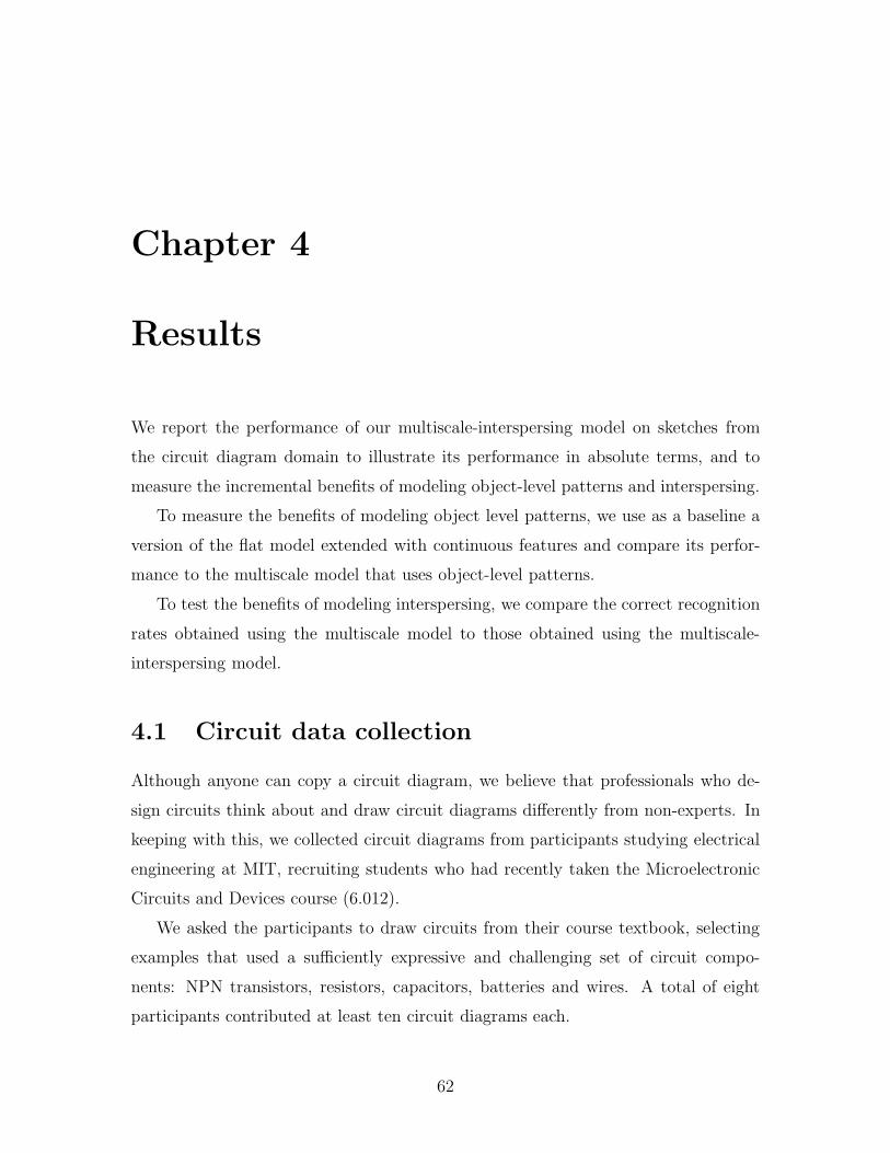
Chapter 4

Results

We report the performance of our multiscale-interspersing model on sketches from

the circuit diagram domain to illustrate its performance in absolute terms, and to

measure the incremental benefits of modeling object-level patterns and interspersing.

To measure the benefits of modeling object level patterns, we use as a baseline a

version of the flat model extended with continuous features and compare its perfor-

mance to the multiscale model that uses object-level patterns.

To test the benefits of modeling interspersing, we compare the correct recognition

rates obtained using the multiscale model to those obtained using the multiscale-

interspersing model.

4.1 Circuit data collection

Although anyone can copy a circuit diagram, we believe that professionals who de-

sign circuits think about and draw circuit diagrams differently from non-experts. In

keeping with this, we collected circuit diagrams from participants studying electrical

engineering at MIT, recruiting students who had recently taken the Microelectronic

Circuits and Devices course (6.012).

We asked the participants to draw circuits from their course textbook, selecting

examples that used a sufficiently expressive and challenging set of circuit compo-

nents: NPN transistors, resistors, capacitors, batteries and wires. A total of eight

participants contributed at least ten circuit diagrams each.

62

Figure 4-1: Examples of collected circuits.

We began by showing participants diagrams of the circuits to be drawn. To ensure

participants got familiar with the circuits, we gave them some time to study each one

until they understood how it worked. To ensure they understood it, we asked them

the function of the circuit (e.g., an inverter circuit, an amplifier), then asked them to

explain verbally how it worked. We then removed the textbook diagram and asked

them to draw the circuit from memory on a Tablet PC, allowing them to consult the

original circuit diagram if needed. Fig. 4-1 shows examples of circuits drawn by the

participants. We manually annotated the sketches to be used as training and testing

data in our experiments.

4.2 Generating an observation sequence

Both training and classification require converting a sketch to an observation sequence

O1:T . Using the early sketch processing toolkit, we first preprocess each sketch to ob-

tain a sequence of primitives P1:T (which in this domain contained only line segments).

Fig. 4-2 illustrates primitive extraction. The pen direction is indicated with arrows

63

Figure 4-2: Conversion to the primitive sequence.

for each primitive.

For each primitive Pt, we obtain an observation vector Ot represented as a five-

tuple (lt, Δlt, θt, Δθt, sgnt) where lt is the length of Pt; Δlt is relative length

(lt/lt−1, 1 for t = 1); θt is the angle with respect to the horizontal axis; Δθt is the

measure of relative angle between Pt and Pt−1 given by the magnitude of the cross

product �u × �v of vectors �u, �v, which in turn are length-normalized versions of Pt

and Pt−1 pointing in the direction of pen movement along each primitive. The only

discrete observable sgnt captures the direction that the stroke turns when moving

from Pt−1 to Pt. It is set to 0 for negative values of �u×�v and 1 for positive values or

t = 1.

For our experiments, we create two datasets: “simple” and “mixed.” The simple

dataset contains only examples without interspersing, while the mixed data contains

both the examples from the simple data set and examples where the user interspersed

strokes during drawing.

4.3 Modeling object level patterns increases recog-

nition accuracy

4.3.1 Experiment setup and quantitative results

For each user, we ran a series of hold-one-out experiments by getting the recognition

rates for each sketch using a model trained on the remaining sketches. For each

sketch, we also trained a baseline system that modeled only stroke-level patterns.

The baseline system has the same computational complexity as our method and was

64

obtained by assigning uniform transition probabilities for the object level:

P (OBJt+1|OBJt,ENDt) =

⎧⎪⎪⎪⎪⎨⎪⎪⎪⎪⎩

1/|OBJ|, if ENDt = true

1 if ENDt = false and OBJt+1= OBJt

0 if ENDt = false and OBJt+1 = OBJt

In both models we used three Gaussian mixtures and set the number of states

for the stroke-level models to 6. We trained them using simple data (because these

models cannot handle interspersing) and tested them on the mixed data (because

that is how the users eventually draw).

Table 4.1 shows the average correct recognition rates for each participant obtained

using the baseline model and the multiscale model. The table also shows the average

and maximum reduction values in the error rates in terms of percentages for each

user. As seen in the table, on average, modeling object-level patterns reduced error

rates between 14% and 37%, and allowed up to 65% of misrecognition errors to be

corrected.1

A paired t-test for the values in Table 4.1 showed the difference to be statistically

significant for p 0.05 and 7 degrees of freedom. We believe such a decrease in the

error would substantially improve users’ satisfaction with the recognition system in

an actual design setting.

4.3.2 Qualitative examples and discussion

We believe it is instructive to explore the kinds of errors avoided by modeling object-

level patterns. Consider Fig. 4-3, an amplifier circuit, which also shows the stroke

ordering for the fragment of the circuit diagram of particular interest to us. Two

interpretations of this circuit are shown in Fig. 4-4.

Fig. 4-4-a shows the interpretation obtained by running the baseline method,

which encounters four recognition errors. The capacitor C2 is misrecognized as wires,

most probably because of the hook hanging off one of the strokes. The NPN transistor

Q2 is misrecognized because the stroke indicating the current direction is noisy. Note

1A misrecognition is defined as computing a value for the object node that disagrees with theground truth.

65

Participant ID1 2 3 4 5 6 7 8

µb 83.2 86.5 85.2 73.8 87.1 90.7 79.1 85.0µm 89.4 89.4 87.3 77.4 89.8 93.0 84.6 88.2Δerr 36.9 21.4 14.1 13.7 20.9 24.7 18.6 21.3maxΔ 65.0 45 31.2 15.0 35.5 40.0 30.7 54.5

Table 4.1: Mean correct recognition rates for the baseline system (μb) and the mul-tiscale model (μm) on sketches collected from 8 participants. The table also showsthe percentage reductions in the error rates and maximum error reductions achievedfor each user as percentages (Δerr and maxΔ). On average, modeling object-levelpatterns always improves performance.

that the vertical part of this transistor (segment #11) and the wire connected to the

emitter (segment #12) are grouped together and labeled as a capacitor. Inspection

of the sketch reveals that these two strokes have roughly the same length and are

sketched one after the other (shown by the numbers in Fig. 4-3). This easily leads

to these strokes being mislabeled as a capacitor.2 Finally, part of the resistor R1 is

misrecognized.

Fig. 4-4-b shows that two of these errors are fixed by the multiscale model. The

multiscale model has learned that the chance of a resistor being followed immediately

by a transistor, and capacitors being immediately followed by resistors with no wires

in between is very small, so these interpretations are penalized. As a result, the two

misrecognitions are avoided.

4.4 Handling interspersings increases recognition

accuracy

4.4.1 Experiment setup and quantitative results

For participants who produced interspersed sketches (#1, #5, #6 and #7), we ran a

series of hold-one-out experiments, comparing the recognition rate of the multiscale-

interspersing model (implemented using features of GMTK[15, 18]) and the multiscale

2This is a result of the limitations of our ordered based recognition.

66

Figure 4-3: One of the circuits drawn by our study participants. Stroke ordering fora fragment of the circuit is indicated by numbers.

Participant ID1 5 6 7

µm 89.4 89.8 93.0 84.6µm−i 92.9 92.2 95.6 87.7Δerr 33.0 23.5 37.1 20.1maxΔ 61.5 33.3 100.0 54.5

Table 4.2: Mean correct recognition rates for the multiscale-interspersing (μm−i) andthe multiscale models (μm) for users who exhibited interspersed drawing behavior.The table also shows the percentage reductions in the error rates and maximum errorreductions achieved for each user as percentages (Δerr and maxΔ). On average,handling interspersing patterns always improves performance.

model. In both models we used three Gaussian mixtures and set the number of states

for the stroke-level models to 6. The DBN representing the multiscale-interspersing

model is shown in Fig. 4-5. We trained the multiscale model using simple data

(because it cannot handle interspersing) and the multiscale-interspersing model using

the mixed data. We tested both models using mixed data.

Table 4.2 shows the average correct recognition rates for each participant obtained

using the multiscale model and the multiscale-interspersing model. The table also

shows the average and maximum reduction values in the error rates in terms of

percentages for each user. As seen here, on average, handling interspersing improves

67

200 300 400 500 600 700

50

100

150

200

250

300

350

400

450

500


(a) Interpretation of the baseline model.

200 300 400 500 600 700

50

100

150

200

250

300

350

400

450

500


(b) Interpretation of the multiscale model.

Figure 4-4: Examples of errors corrected using context provided by object-level pat-terns. There are four misrecognitions in (a). Note how two of these misrecognitionsis fixed using knowledge of object level patterns (resistor in the upper left corner (R1)and the wire connected to the emitter of the misrecognized transistor). See Fig. A-2for B&W printing.

68

Figure 4-5: The dynamic Bayesian network representing the multiscale-interspersingmodel that handles interspersed drawing.

performance, and allows 20%-37% of misrecognition errors to be corrected.

A paired t-test for the values in Table 4.2 found the difference to be statistically

significant for p < 0.05 and 3 degrees of freedom.

4.4.2 Quantifying errors per-interspersing

The percentages presented above do not show the full extent of the negative effects

of not handling interspersing because the percentage of errors due to interspersing

is diluted by the large number of other components successfully recognized. A more

informative measure of the benefits of handling interspersing can be obtained if we

look at the number of misclassified primitives per interspersed primitive.

In order to measure this, we ran both the multiscale model (the baseline) and

the interspersing-multiscale model on a control group that contained ten sketches

with no interspersing, and a test group that contained versions of these sketches with

interspersings. The interspersed version of each sketch was obtained by moving one

of the wires preceding/following a transistor back/forward in time. Our use of these

examples ensures that we measure the misrecognition effects due only to interspersing.

We trained our baseline model with the non-interspersed data and supplied the

69

Sketch ID1 2 3 4 5 6 7 8 9 10 μ

Total primitives 90 85 104 101 92 100 87 105 80 98 94.2Added interspersings 2 2 4 4 3 3 2 2 2 4 2.8

Missed by the baseline 7 9 15 12 12 12 13 13 11 19 12.3Missed by our model 3 3 4 1 0 0 2 2 2 3 2

Difference 4 6 11 11 12 12 11 11 9 16 10.3Missed prim./intersp. 2 3 2.75 2.75 4 4 5.5 5.5 4.5 4 3.8

Table 4.3: This table shows the number of misrecognized primitives per interspersing.The first two row shows the number of total primitives in each sketch and the numberof added interspersings. Next two rows show the number of primitives incorrectlyrecognized by the baseline and by our model. The next row shows the number ofprimitives that the baseline misses because it cannot handle interspersings and thelast row is the number of primitives missed by the baseline per interspersing.

interspersing-multiscale model with the additional interspersed examples. Table 4.3

shows the number of misrecognized primitives per interspersing. The first two rows

show the number of total primitives and the number of added interspersings per

sketch. The table also shows the total number of primitives incorrectly recognized by

the baseline and by our model. The last two rows show the total of primitives that the

baseline misses because it cannot handle interspersings and the number of primitives

missed by the baseline per interspersing. As seen in the table, a single interspersing

causes as many as 16 primitives to be misclassified. Considering that a transistor has

five primitives, this is worth about three transistors. When we normalize the number

of misrecognized primitives per sketch by the number of interspersings we get about

2-6 misrecognized primitives per interspersing.

In the best case, the errors caused by each interspersing will require at least one

correction by the user (e.g., when all the misrecognized shapes belong to the same

shape). In the worst case, the errors may require as many corrections as the number

of misclassified primitives, further showing the utility of modeling interspersing.

4.4.3 Qualitative examples and discussion

Fig. 4-6 shows an example illustrating how interspersed drawing causes misrecog-

nitions if not handled properly. This example is particularly instructive because it

70

Figure 4-6: Another circuit drawn by our study participants. Stroke ordering for afragment of the circuit is indicated by numbers.

shows that interspersing only a single primitive can lead to a cascade of misrecog-

nitions. In this example, the user drew the collector of the transistor Q2 and the

wire connected to it using a single stroke (stroke #15, which is also an example of

multi-object stroke).

Two interpretations of the circuit are shown in Fig. 4-7. Fig. 4-7-a shows the

interpretation obtained by running the multiscale model. In this figure, there are two

recognition errors. Q2 is misclassified as a set of wires, and the two wire segments

connected to the base are misclassified as a resistor.

Fig. 4-7-b shows that both errors are fixed when we use the multiscale-interspersing

model. The multiscale-interspersing model has learned that with probability 0.14

wires can be drawn in the course of drawing a transistor. This not only allows the

transistor to be identified correctly but also helps the two wire segments to be clas-

sified correctly by using the knowledge that transistors very rarely proceed resistors,

P (OBJt=NPN | OBJt−1=RESISTOR) ≈ 0. This example shows the benefits of mod-

eling both object-level patterns and interspersing.

The incremental benefits of using a more elaborate model may appear at times to

be small (e.g. Fig 4-8). Nevertheless, correcting each misclassification requires effort

on the part of the user and gets in the way of getting the job done. Hence we believe

the error reduction rates we have demonstrated are significant in the context of a

sketch-based user interface.

71

100 200 300 400 500 600 700 800 900

−100

0

100

200

300

400

500


(a) Interpretation of the multiscale model.

100 200 300 400 500 600 700 800 900

−100

0

100

200

300

400

500


(b) Interpretation of the multiscale-interspersing model.

Figure 4-7: In this example, the user interspersed a wire connected to the collector ofthe transistor on the right. As a result the transistor is misclassified by the multiscalemodel (a). The multiscale-interspersing model identifies the wire interspersing (in-dicated by black) and correctly interprets the transistor (b). See Fig. A-3 for B&Wprinting.

72

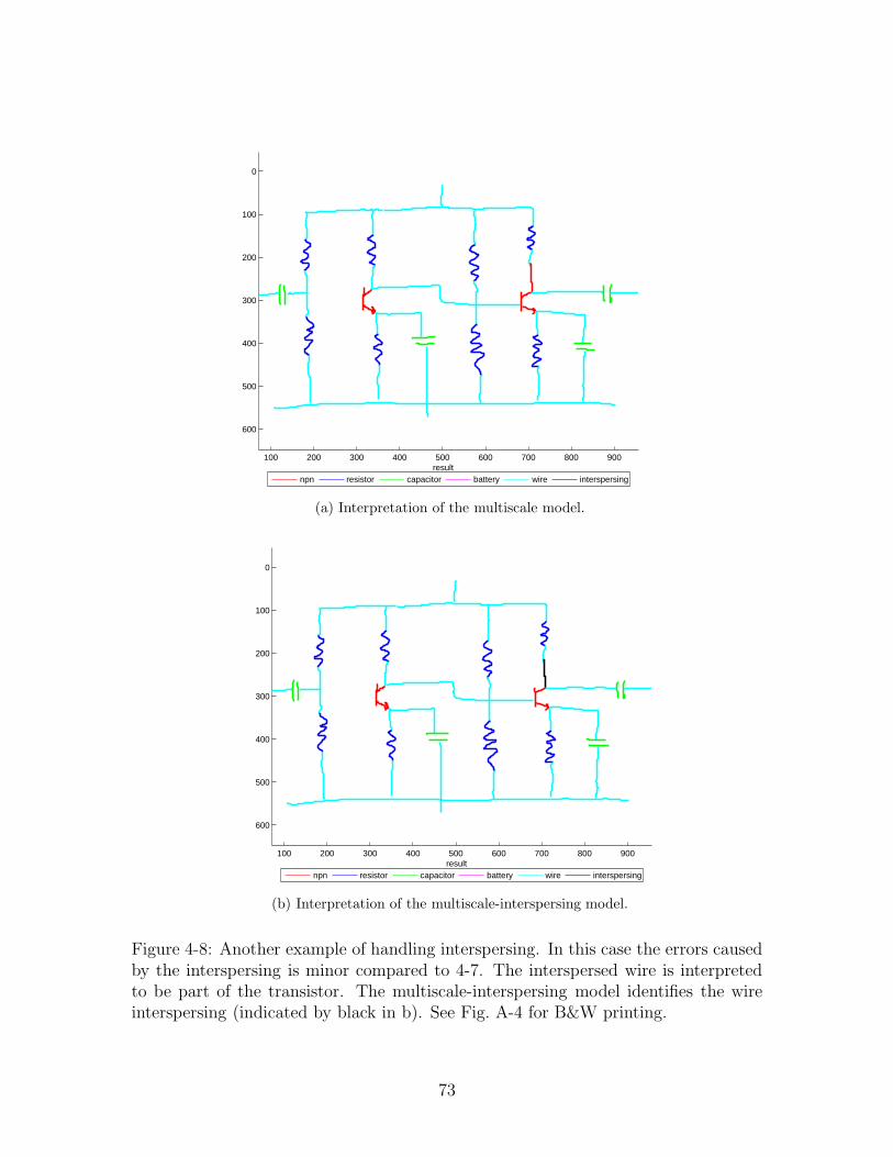
100 200 300 400 500 600 700 800 900

0

100

200

300

400

500

600



100 200 300 400 500 600 700 800 900

0

100

200

300

400

500

600



Figure 4-8: Another example of handling interspersing. In this case the errors causedby the interspersing is minor compared to 4-7. The interspersed wire is interpretedto be part of the transistor. The multiscale-interspersing model identifies the wireinterspersing (indicated by black in b). See Fig. A-4 for B&W printing.

73

4.5 Summary

We have demonstrated that it is possible to recognize sketches using temporal patterns

that naturally appear during sketching. This is particularly noteworthy because until

recently, time-based graphical models were considered to be unsuitable for sketch

recognition [5].

The results we have presented above show that using object-level temporal pat-

terns increases recognition rates by incorporating contextual information about object

orderings. We also showed that explicitly modeling interspersed drawing behavior in

a principled way allows us avoid cascades of misinterpretations often caused by inter-

spersings.

Finally, we note that the baseline models that we described are easier to implement

compared to our main model. This gives designers the choice to work with easier

to implement methods at the cost of sacrificing expressiveness of the model and

recognition accuracy.

74

Chapter 5

Related work

Work in pen-based systems goes back to the 1970’s [94, 57]. Although the potential

impact of having computers interpret free-hand input was recognized early on, much

of the early work suffered from ad-hoc recognition strategies and too many constants

that need to be tuned. Nevertheless, early systems have been helpful in understanding

what makes sketch recognition challenging. With the recent development of machine

learning theory, well-founded statistical approaches to sketch recognition have been

introduced. From a historical perspective, the goal of this thesis has been to contribute

in this direction.

This chapter positions our work within the recent pen-based systems research and

recognition systems. We discuss the related work under three groups:

• Recognition systems include speech, graphics and object recognition systems.

These are relevant in the context of sketch recognition because in both cases

the task is to interpret noisy signals, and approaches to recognition have a great

deal in common.

• Pen-based interfaces are systems that aim to support natural interaction by

supporting some degree of pen input. Although most of these systems process

the pen input to some degree, the amount of recognition is too limited to call

them sketch recognition systems. These systems focus mostly on the user inter-

face aspects of pen-based interaction and recognition is often not their primary

concern or the intended contribution.

75

• Sketch recognition systems are most relevant for the work we presented. We

discuss sketch recognition systems under two categories, those that use spatial

features and those that use temporal features.

5.1 Recognition systems

Other recognition problems are relevant to sketch recognition because many common

themes appear in both cases such as noisy input, feature representation, choice of

learning machinery.

5.1.1 Speech and handwriting recognition

Speech recognition systems model speech as sequence data. Use of statistical models

for sequential data such as hidden Markov models has gained popularity after their

success in speech recognition tasks [99]. Recently dynamic Bayesian networks have

also been used for recognition. The advantage of DBNs is their ability to model

dynamic processes using distributed state representations [15].

Handwriting recognition and online handwriting recognition work also use time

based statistical models heavily [71, 98] although there is little work based on syntactic

methods [86, 65, 70].

The handwriting recognition community has also come up with a large number of

methods for recognizing single stroke or segmented pen input using HMMs and the

single gesture recognition problem is mostly considered to be solved.

Both speech and handwriting recognition systems can take advantage of a vast

number of robust preprocessing and segmentation methods (e.g., silence detection and

word boundary detection). This reduces the computational cost of speech recognition

[110] and results in increased recognition accuracy for handwriting recognition [25]

systems because they can run individual classifiers on isolated characters. This is in

contrast with sketch recognition where there is no segmentation strategy that will

work for multiple domains at the signal level.

76

Figure 5-1: An example illustrating the kinds of input that graphics recognitionsystems accept. Here is a typical input for the graphics recognition system describedin [82] and the processing of the system.

5.1.2 Graphics recognition

Graphics recognition aims to recognize computer generated diagrams [123, 82, 11,

114]. The input is a scan of a computer generated diagram (usually a CAD model).

The output is either the vectorized version of the shapes, or a segmented and classified

version of the input. The most important difference between graphics recognition

and sketch recognition is the availability of clean and precise input for the graphics

recognition task. Fig. 5-1 illustrates the kind of input that graphics recognition

systems deal with. The figure shows the input for the graphics recognition system

described in [82] and the processing of the system. Compared to sketch recognition the

input to graphics recognition is cleaner and more precise, thus the recognition problem

is better understood and it is easier to achieve high recognition rates using standard

computer vision techniques. For the same reason, graphics recognition techniques

don’t transfer well to hand drawn diagrams.

5.1.3 Object recognition

Although the object recognition research is not relevant to the temporal model that

we have presented, many sketch recognition algorithms are based on structural and

syntactic methods (e.g., work in [4, 5, 107] and [84] use structural recognition strate-

77

gies while [53, 52, 51] and [84] describe syntactic shape description languages).

Structural pattern recognition methods (also known as model-based or template-

based methods) formulate the recognition problem based on implicit or explicit rep-

resentations of objects in terms of their structure (i.e., components, sub-components

and their relationships). In structural object recognition, models describe objects in

terms of primitives and relationships between primitives (constraints). In the com-

puter vision literature, models are also referred to as templates, and model features

are referred to as template slots or slots. Primitives of the model are called model

features, and primitives forming the scene are called scene features. Model and scene

features need not be exactly the same. For example, 3D model edges may appear as

2D edges in the scene, but they are related by some function (translation, rotation,

projection). The scene features include primitives originating from the objects in the

scene that we would like to recognize, and may also contain spurious features. 1

Syntactic approaches form a subset of structural approaches where the relation-

ships are specified using a grammar [23, 113, 42]. Early work in in structural recog-

nition is also related closely to CAD-based recognition [55, 60, 46, 10, 24, 39] and

constraint satisfaction [115]. The syntactic methods on the other hand are related to

visual languages two dimensional parsing [88]. In the sketch recognition community,

[104] and [51] describe ways of compiling object descriptions to automatically gener-

ate recognizers. These techniques are more appropriate for graphics recognition tasks

as outlined above because sketches are not clean and precise as required by these

algorithms.

Other examples of object recognition algorithms include those that use constraints

for efficient matching. The matching can be in the correspondence space [47, 81, 37,

38, 48] or in the transformation space [26].

Later work in computer vision intensively uses machine learning methods to learn

statistical models from data. Some of the relevant work includes two-dimensional

HMMs [77, 76] Bayesian networks [69, 78] and undirected graphical models for recog-

nition that use Markov random fields [28] introduced by Geman and Geman [44].

As we describe in section 5.3, the main drawback of sketch recognition systems

1Spurious features are features originating from unknown objects or from errors made at the lowlevel processing stage (i.e., edge detection, feature point detection).

78

based on computer vision techniques is the high computational cost of matching in

presence of noise and imprecision that is specific to sketches. Although suggestions

have been made to make matching more efficient by pruning the search space, such

improvements always come with limiting assumptions.

5.1.4 Symbol recognition systems

Most sketch based systems assume that the users draw one object at a time (no

interspersing) and specify the proper segmentation implicitly (e.g., by pausing for a

certain amount of time between objects) or implicitly (e.g., pressing a button after

drawing each object). These systems employ symbol recognizers to classify the already

segmented objects. These systems are either gesture based or shape based. From a

user’s point of view, a shape based recognizer is usually preferable because it doesn’t

require the user to learn a prespecified gesture vocabulary.

The gesture recognizer described in [102] is perhaps the most popular method

used for gesture based input. Its most severe limitation is the lack of support for

multi-stroke gestures. The work by Apte et al. and Fonseca et al. describe ways

of extending gesture based input to use multiple strokes [9, 87, 7, 29], but they still

require isolated objects (e.g., no segmentation is performed).

Some of the shape based recognizers include the SVM-based active learning sys-

tem developed by Sun et al. [111] and the recognition system being developed by

Oltmans [95]. Oltmans’ system uses a feature representation based on shape contexts

originally developed by Malik et al. [13] and a learning framework based on SVMs

to do recognition. Watanabe et al. describe a pattern representation and recognition

scheme that uses data compression [67, 121]. Another symbol recognition system is

based on Zernike moments described by Hse et al. [58]. In [64] Kara et al. describe

a symbol recognizer using and image-based approach.

The shape based recognizers are appropriate for sketching interfaces where no

segmentation is required. We believe requiring the user to actively participate in the

segmentation process in ways described above interferes with the task at hand will

result in unnatural interfaces. It is much more desirable to have a system that can

do segmentation automatically such as ours.

79

5.2 Pen-based interfaces

5.2.1 Early processing systems

Systems that process pen input at the lowest level for the purposes of shape repre-

sentation and feature point detection form the foundation of most sketch recognition

systems. Work in [14, 103, 12, 105] are examples of such systems that specifically deal

with freehand input. In addition, there is a wealth of work in the computer vision

community that deal with issues of feature point detection, shape approximation and

perceptual grouping [100, 79, 80]. Work in [35] and [105, 120] are examples of systems

that try to detect regularities and symmetries in the input at the geometric-level and

perform adjustments by mapping near-singular properties to singular properties. Our

work uses the early sketch processing toolkit in [105].

5.2.2 Computer graphics and user interface applications

Systems that support pen-based interaction include computer graphics oriented sys-

tems that are intended for 2D and 3D rapid geometric design [35, 59, 124, 32, 97, 54].

These systems allow specifying geometric shapes and constraints using free-form ink

and illustrate the potential of combining free-hand input with relatively little recog-

nition to specify geometry in a design setting.

Other systems that support some form of pen input include [41], a gesture based

system for entering music notation, the sketch-based GIS system by Blaser [20], and

the Electronic Cocktail Napkin by [49, 50]. SILK [73] describes a gesture-based

approach to interface design. Quickset [27] describes a multimodal interaction frame-

work that supports gesture-like pen input.

Others have explored sketching in the context of multi-modal input fusion [40, 27,

2, 63, 96, 33, 31]. While [27] describes a general framework for multimodal fusion, [2]

and [96] describe how speech can be combined with sketching and [33] investigates

ways of using speech, gestures and sketching as complementary information sources

in a multimodal interaction setting.

Although the systems described so far have some support for pen input, they

have limited recognition capabilities and are thus not sketch recognition systems in

80

the sense used in this thesis. A vast majority of these systems support only single

stroke objects or gesture-like input. Most of them are built on the premise that the

users know about the limitations of the system and will draw accordingly. Examples of

this include having the user indicate appropriate segmentation by pausing or explicitly

by clicking a “done” button. The lack of emphasis on recognition in these systems

is balanced by their focus on the human-computer interface issues of sketch-based

interaction.

There is also some work that does not present sketch recognition techniques but

addresses general user interface issues [21, 61, 62, 40, 72]. Other work in [1] describes

appropriate gestures selection strategies for gesture based systems. A sketch descrip-

tion language developed by Hammond investigates issues such as structural shape

description, editing behavior and display options [53, 52, 51]. This body of work is

relevant for future work on exploring general HCI issues as we describe below.

5.3 Sketch recognition systems

Work in sketch recognition can be divided into two groups based on whether it uses

temporal features. We start with a review of the large body of work that does not

use temporal features. These systems are complementary to our approach. Then we

discuss those that use temporal features for recognition.

5.3.1 Use of spatial data for recognition

Early work that uses spatial constraints for sketch recognition includes work by Weis-

man and Muzumdar [122, 93] and the ASSIST system by Alvarado [3] focus on inter-

preting hand-drawn two dimensional sketches of mechanical devices. These systems

have been demonstrated to be usable by experienced users (e.g., the developers).

The stick-figure interpretation system by Mahoney and Fromherz [84, 85, 83] uses a

structural language for describing objects and a constraint-based matching approach.

Their work is the first to investigate the computational complexity of model-based

sketch recognition. They present heuristics such as grouping, anchors, salience and

model bias for speeding up the matching. They also identify some of the messiness in

sketches as being due to overshooting, undershooting, and failure of co-termination.

81

Given a sketch, their algorithm first generates an attributed graph representing the

scene using the set of lines in the sketch and their relationships. Next, the scene graph

is augmented by subgraphs corresponding to possible ambiguities in the interpretation

of line relations. This augmentation operation – called graph elaboration – applies

perceptual organization principles such as good continuation and proximity. Next, the

algorithm looks for instances of the model graph in the scene graph by performing

subgraph matching. This approach to sketch recognition can be thought of as an

adaptation to sketches of the subgraph isomorphism approach, popular in computer

vision, in a way that deals with the free-hand and noisy characteristics of sketches

using perceptual organization principles. On the other hand, because the subgraph

isomorphism treats the sketch as a static image, this approach does not capitalize on

the dynamic properties of sketches such as the drawing order of strokes.

Shilman et al. describe a statistical, grammar based ink parsing algorithm for

sketch recognition [107]. In this framework, the system designer describes objects

with a declarative grammar and gives labeled training examples. The initial grammar

requires predetermined constants for computing constraints between objects. A parser

is generated using this information. During runtime, the parser looks at the sketching

surface and generates a parse tree whose nodes correspond to alternate interpretations

of the sketch. Next, Bayesian networks corresponding to interpretations at the parse

tree nodes are generated. Most likely interpretations are chosen and expanded further,

pruning nodes with probabilities less than a preset threshold. The authors report that

their method outperforms a hand-coded parser for a domain with a relatively simple

grammar. Having been inspired by language parsing, this approach is not built with

the dynamic and interactive nature of sketching in mind.

Viola et al. describe a spatial recognition and grouping method for text and

graphics [108, 106]. They use a discriminative classifier to classify connected sub-

graphs of a proximity graph constructed from the sketch. Each subgraph is classified

as either making up an object or as an invalid stroke combination. They select a

small subset of efficient features and perform an A∗ search over connected subsets to

find the optimal segmentation and recognition of all strokes on the page. In order

to keep the search tractable they make some assumptions about the objects in the

domain. For example, they assume that objects in their domain have no more than

82

8 strokes, or that the strokes constituting an object are within a certain distance.

These assumptions seem to work for flowchart-like drawings where the connectors

and objects are sufficiently separated from one another, but the practicality of these

algorithms is yet to be demonstrated in general for domains where objects vary in

size and shape where assumptions on the object size and scale may not hold.

Work by Alvarado describes a blackboard based architecture with a top-down

recognition component based on dynamically constructed Bayesian networks that

allows recovery from bottom-up recognition errors [4, 5, 6]. This system also uses a

structural approach to recognition. A major strength of this system, which makes it

unique with respect to the other recognition systems, is its ability to model low-level

errors explicitly and use top-down and bottom-up information together to fix errors

that can be avoided using context. This strength comes with a computational cost

that prevents the system from running in real-time despite some limiting assumptions

made and despite the use of efficient search strategies to prune the hypothesis space.

In most cases the system takes several minutes to hours to process moderate size

drawings. Also, although this system uses a probabilistic model based on dynamically

constructed Bayesian networks, the object models have to be specified by an expert

instead of learning them from data. One can also argue the other way saying that

using expert knowledge is a strength of this system, but our experience seems to

indicate that hand tuning probabilities is hard and time consuming even for experts,

whereas creating moderate amounts of training data (as it was required in our case)

is more straightforward and requires almost no expertise.

In [45], Kara et al. present a circuit diagram recognition system that does seg-

mentation using a heuristic called “ink-density” and runs isolated symbol recognizers

to generate an interpretation. Their system has as number of strengths such as fast

recognition, support for multi-stroke objects and multi-object strokes and arbitrary

stroke orderings within each object. On the other hand the segmentation algorithm

used in this work does not handle interspersed drawing, so the user is required to fin-

ish an object before starting a new one. It is also not clear how well the segmentation

algorithm based on ink density would work for other domains (e.g., UML diagrams

or course of action drawings).

Finally Szummer et al. [68] describe a generative Bayesian framework for shape

83

recognition. They use dynamic programming to achieve segmentation and classifica-

tion simultaneously. The major strength of their approach is the ability to recognize

messy drawings using single examples by assuming a Gaussian noise model. As was

the case for some of the approaches described above, the authors make certain as-

sumptions to keep the search for the optimal segmentation tractable. Specifically they

assume that each subset of stroke fragments considered during segmentation contains

no more than seven straight line segments. This might be a severe limitation in do-

mains with moderately complex objects, such as the sloppy stick-figures considered

by Mahoney et al. [84, 85, 83] or the course of action diagrams domain.

5.3.2 Use of temporal data for recognition

This thesis is the first to use temporal patterns for sketch recognition. Some of the

related work includes the work in the handwriting recognition community where a

large number of methods to recognize single stroke or segmented pen input using

HMMs. In the sketch recognition community, work in [8] describes an HMM-based

symbol recognizer that uses chain-code-like features to recognize isolated symbols.

Our work does not assume segmented input and builds a joint model for complete

sketches.

In [109], the authors present a sketch interpretation and curve refinement system

that uses an HHMM setup. This work shares the same motivation as ours. In their

work, they assume that the parameters of the object-level process (which they refer

to as the scene level) is supplied by the user using a semantic graph representation.

We learn the parameters of the stroke-level and object-level patterns from data, and

use the more efficient DBN representation to avoid the O(T 3) complexity of HHMMs.

Furthermore, we support multi-stroke objects and real-valued continuous observations

which allow using a rich set of features.

84

Chapter 6

Contributions

6.1 Contributions

We have presented a sketch recognition framework that exploits both stroke-level and

object-level temporal orderings. Our framework allows learning object-level patterns

from data, handles multi-stroke objects and multi-object strokes efficiently, supports

continuous observable features and handles interspersed drawing.

A number of contributions make our work unique:

• Our work is the first to demonstrate the utility of stroke ordering information

and the suitability of time-based graphical models for recognizing complicated

sketches and is particularly noteworthy because until recently such models were

considered to be unsuitable for sketch recognition [5].

• We showed how graphical models can be used to implement our model of tem-

poral patterns efficiently using features such as switching parents, sparse rep-

resentations and parameter tying. Our model interprets sketches with several

dozen objects under a second on a standard PC, and as such is suitable for

real-time sketch interpretation.

• We reported that a standard implementation of belief propagation, appropriate

for simple conditional Gaussian belief networks, runs into numerical instabilities

when used for inference in our model. We noted that the Lauritzen-Jensen stable

85

conditional Gaussian belief propagation algorithm should be used to avoid such

numerical problems in recognition.

• We demonstrated that our hierarchical models capture knowledge of both com-

mon stroke orderings and common object orderings. Our evaluation involving

circuit diagrams collected from eight participants shows that modeling common

object orderings reduces the number of recognition errors by 14%- 37%.

• We also showed how a probabilistic temporal model can explicitly model in-

terspersed drawing behavior. Interspersed drawing behavior poses serious chal-

lenges to a naıve approach of temporal sketch recognition model, but we ad-

dress the issue remaining within the formal framework of Dynamic Bayesian

Networks. Therefore we do not rely on the the assumption that users to draw

objects one at a time. We showed that modeling interspersing reduces recogni-

tion errors by an additional 20%-37%.

• Our recognition framework allows strokes to be part of multiple objects as long

as objects do not share primitives. We support multi-stroke objects and objects

with variable number of components (e.g., resistors with variable number of

humps).

• Finally we support discrete and real-valued feature representations that allows

us to encode our data using discrete encodings for categorical properties (e.g.,

a stroke being a circle vs. a line), and real-valued encodings for continuous

features (e.g., length, orientation of a line).

6.2 Discussion

We believe that our approach to modeling multi-scale patterns in presence of inter-

spersing can be applicable to a number of other problems that deal with temporal

data and use a sequence based representation. Fundamentally, the probabilistic model

that we have presented is not specific to sketching data and it can handle any kind of

sequence data where the Markov assumption and a representation based on dynamic

Bayesian networks is appropriate.

86

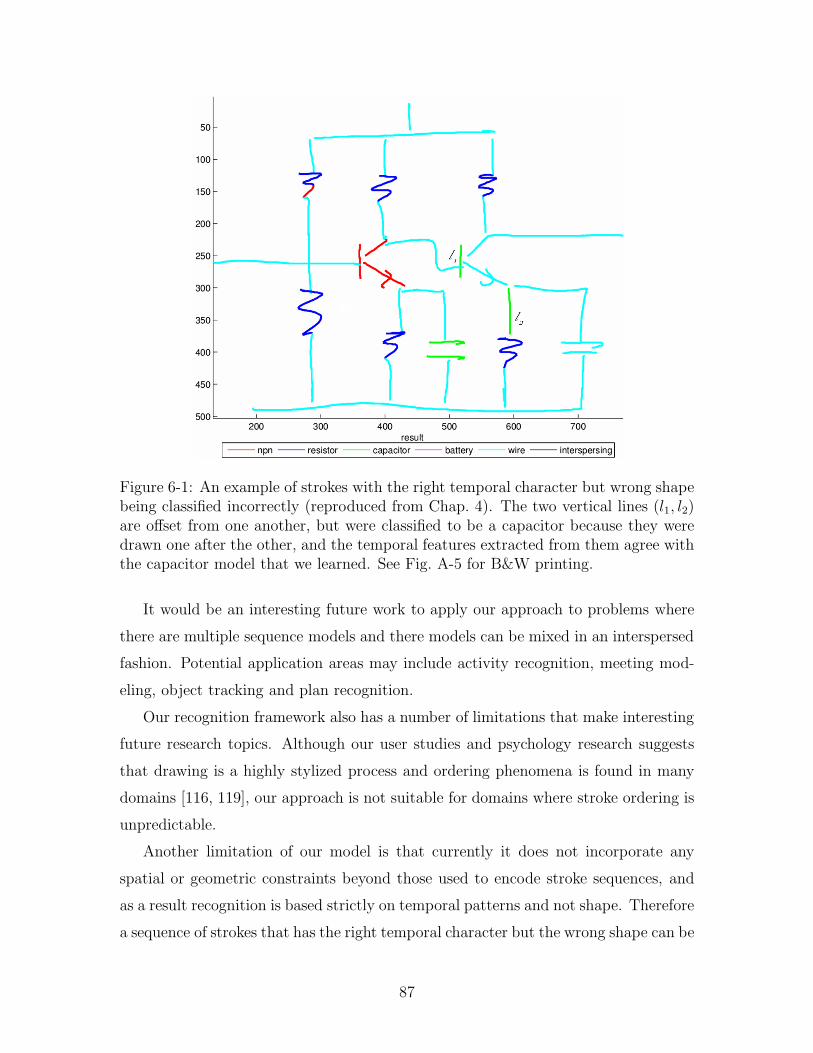
Figure 6-1: An example of strokes with the right temporal character but wrong shapebeing classified incorrectly (reproduced from Chap. 4). The two vertical lines (l1, l2)are offset from one another, but were classified to be a capacitor because they weredrawn one after the other, and the temporal features extracted from them agree withthe capacitor model that we learned. See Fig. A-5 for B&W printing.

It would be an interesting future work to apply our approach to problems where

there are multiple sequence models and there models can be mixed in an interspersed

fashion. Potential application areas may include activity recognition, meeting mod-

eling, object tracking and plan recognition.

Our recognition framework also has a number of limitations that make interesting

future research topics. Although our user studies and psychology research suggests

that drawing is a highly stylized process and ordering phenomena is found in many

domains [116, 119], our approach is not suitable for domains where stroke ordering is

unpredictable.

Another limitation of our model is that currently it does not incorporate any

spatial or geometric constraints beyond those used to encode stroke sequences, and

as a result recognition is based strictly on temporal patterns and not shape. Therefore

a sequence of strokes that has the right temporal character but the wrong shape can be

87

classified incorrectly. For example, the two parallel strokes in Fig. 6-1 were classified

as a capacitor, even though the strokes were offset from one another. We consider

below how this limitation can be addressed by using shape based classifiers as external

sources of information.

88

Chapter 7

Future work

Future directions for this research include exploring alternative approaches to some

of the issues noted above, including other models for handling interspersing. There

are also a number of problems that require further research such as finding ways of

incorporating other knowledge sources into the decision process and exploring some

of the user interface issues.

7.1 Alternative models of interspersing

As noted above, we framed our approach for handling interspersing based on our

observations about the domains that we studied including those mentioned in Chap. 2

(finite state machines, UML diagrams, Course of Action Diagrams, stick-figures and

emoticons) and circuit diagrams, which was our domain of choice for evaluation. In

these domains, we never observed an object of the same type being interspersed (e.g.,

interspersing two transistors), and as a result our model doesn’t handle such cases. It

would be an interesting exercise to investigate the drawing patterns in other domains

to see if any of them contain interspersings of the same object type. If that is indeed

the case, then what is the best way of modeling such interspersings?

One possibility would be to stay within the framework we have introduced and

add an extra stroke level model for the object class that has self interspersing. For

example, assume we have a scenario where the user starts drawing another NPN

transistor before finishing the current transistor. In this case our DBN model would

89

Figure 7-1: One plausible way of modeling self interspersing could be to duplicate thestroke level model for the self interspersing class. In this case, we assume a scenariowhere the user intersperses two transistors, so we have the N node as usual and anextra node IN to represent the stroke-level model for the interspersed NPN transistor.

have the N node as usual and an extra node IN to represent the stroke-level model for

the interspersed NPN transistor (Fig. 7-1). The parameters that capture the stroke-

level patterns would be the same for both models (i.e., we assume the user draws an

interspersed transistor similar to a regular transistor). This would allow us to learn

one stroke-level model for the N and IN nodes, and have a compact representation

using parameter tying.

Another approach might be to have two separate multiscale models (as described

in section 3.6) and a binary switching parent node that activates only one of these

models at given time. The first multiscale DBN fragment would track the joint state

of the generative process1 without interspersing as usual, and the second fragment

would get activated when there is an interspersing. The joint state of the first frag-

ment would keep the information needed to resume the generative process once the

interspersing is over. Obviously many interesting research issues need to be addressed

1In this case the joint state would include knowledge of what object is being drawn and the stateof the stroke level generative process.

90

in such a framework including the tractability of inference.

7.2 Incorporating other knowledge sources

Another interesting direction to explore would be to find ways of incorporating infor-

mation from external knowledge sources. The mechanism used to incorporate external

information could be different based on the nature of the supplied information. For

example, if the source of the information is the user (e.g., the user explicitly indicat-

ing the classification for a set of strokes), then we can take the information as ground

truth and incorporate it in the inference mechanism as observed values.

7.2.1 Incorporating user feedback

Assume the user drew the circuit in Fig. 7-2 and the recognition system misclassified

the circled strokes. Now, if the user selects these strokes and labels them explicitly

as forming a capacitor, we can take this information as ground truth and inject it

directly into our DBN model by making certain nodes in the unrolled DBN observed.

Specifically, the MUX and the END nodes corresponding to the two strokes become

observable (see Fig. 7-3). Because the the user identified the two strokes as a capaci-

tor, the MUX nodes corresponding to these strokes become observable. Also, because

there is no interspersing in our domain, it must be the case that the user has just

finished drawing an object before the capacitor and will start a new object next (thus

the three END nodes are now observed). Once the values of these nodes are injected

into the unrolled DBN, we can perform inference which will potentially cause some of

the other errors to be corrected once the effects of these observations are propagated

to the neighboring nodes (indicated by dotted circles).

7.2.2 Incorporating information from external classifiers

If the external knowledge source is a potentially unreliable external classifier, then it

should be treated as a noisy observation. One way of achieving this would be to use

the information provided by the external classifiers as soft evidence [118] or virtual

evidence [101] by having a child node associated with each MUX node (e.g., Fig 7-4).

91

Figure 7-2: Suppose the user drew the above circuit diagram and the recognitionsystem misclassified the circled capacitor. Now, if the user selects these two strokesand labels them explicitly as forming a capacitor, then we can take this informationas being ground truth. This allows us to inject this information directly into ourDBN model by making certain nodes in the unrolled DBN observed (see Fig. 7-3).

Figure 7-3: If the user explicitly corrects a misrecognition as describe in Fig. 7-2,then this makes certain nodes in the unrolled DBN observable (nodes circled withdashed lines). When we perform inference with the new observed values, the effectsof the observations will propagate to the neighboring nodes (nodes circled with dottedlines).

92

Figure 7-4: One way of incorporating information from external classifiers would beto use the provided information as soft evidence [118] or virtual evidence [101] byhaving a child node associated with each MUX node as shown here. The EC nodecarries information supplied by the external classifiers.

This would also serve as a step toward combining temporal and spatial/structural

information for sketch recognition.

7.3 Incorporating spatial features

As mentioned in section 6.2, our temporal model does not incorporate any spatial or

geometric constraints beyond those used to encode stroke sequences, and as a result

recognition is based strictly on temporal patterns, not shape. Therefore a sequence

of strokes that has the right temporal character but the wrong shape can be classified

incorrectly. One way to remedy this shortcoming would be to combine spatial and

temporal models. As mentioned in section 3.5.4, if there is no interspersing, an ap-

proach based on dynamic programming can be used to combine spatial and temporal

constraints. A more challenging task is to find ways of combining two information

sources when there is interspersing or detecting when the user is employing a novel

stroke ordering such that the spatial features are given heavier emphasis. This is an

interesting avenue that we plan to pursue.

93

7.4 User interface issues

Finally, in this thesis we focused entirely on recognition issues and did not address

any user interface issues. Because our approach uses temporal features only, its failure

modes may be different from those of a system that uses geometric constraints. It

would be useful to investigate whether this is the case, and what the implications are

from a user-interface point of view (e.g., do methods for error correction transfer to

this new way of recognition).

94

Appendix A

Recognition results for non-color

printing

Figure A-1: In this example, the user interspersed a wire connected to the collectorof the transistor Q2. We present a model that can recognize objects correctly evenin the presence of such interspersings and identify interspersed objects (indicated byI-W).

95

(a) Interpretation of the baseline model.

(b) Interpretation of the multiscale model.

Figure A-2: Examples of errors corrected using context provided by object-level pat-terns. There are four misrecognitions in (a). Note how two of these misrecognitionsis fixed using knowledge of object level patterns (resistor in the upper left corner (R1)and the wire connected to the emitter of the misrecognized transistor).

96



Figure A-3: In this example, the user interspersed a wire connected to the collectorof the transistor on the right. As a result the transistor is misclassified by the multi-scale model (a). The multiscale-interspersing model identifies the wire interspersing(indicated by I-W) and correctly interprets the transistor (b).

97



Figure A-4: Another example of handling interspersing. In this case the errors causedby the interspersing is minor compared to 4-7. The interspersed wire is interpretedto be part of the transistor. The multiscale-interspersing model identifies the wireinterspersing (indicated by I-W in b).

98

Figure A-5: An example of strokes with the right temporal character but wrong shapebeing classified incorrectly (reproduced from Chap. 4). The two vertical lines (l1, l2)are offset from one another, but were classified to be a capacitor because they weredrawn one after the other, and the temporal features extracted from them agree withthe capacitor model that we learned.

99

Appendix B

Symbols used

S = S1, S2, ...SN A sketch, defined as a sequence of strokes.

P = P1, P2, ...PT The sequence of time-ordered primitives obtained from S .

C = {C1, C2, ...Cn} The set of classes.

G = G1, G2, ...GK The set of groups identified by the segmentation process.

L = L1, L2, ...LK Labels for the groups (Li ∈ C ).

Gi = ρ1, ρ2, ...ρn Indices of the primitives included in group Gi sorted in ascending order.

� All possible groupings of the primitives in a sketch.

�(G) All possible labelings of a group.

OGiThe sequence of observations corresponding to a group of primitives Gi.

λL(Gi) Model corresponding to the label assigned to the primitives in group Gi.

λ(A, B, π) A Hidden Markov Model.

100

A Transition matrix for the HMM.

B Observation matrix for the HMM.

π Prior for the HMM.

(B1, B�) A dynamic Bayesian network.

B1 Initial frame for the dynamic Bayesian network.

B�

Repeating frame for the dynamic Bayesian network.

101

Bibliography

[1] James A. Landay A. Chris Long, Jr. and Lawrence A. Rowe. ‘those look similar!’

issues in automating gesture design advice. PUI, November 15-16, 2001.

[2] Aaron Adler. Segmentation and alignment of speech and sketching in a design

environment. Masters Thesis, Cambridge, Massachusetts Institute of Technol-

ogy, February 2003.

[3] Christine Alvarado. A natural sketching environment: Bringing the computer

into early stages of mechanical design. Master’s thesis, Massachusetts Institute

of Technology, 2000.

[4] Christine Alvarado. Sketchread: A multi-domain sketch recognition engine. In

Proceedings of ACM Symposium on User Interface Software and Technology,

2004.

[5] Christine Alvarado and Randall Davis. Dynamically constructed bayes nets

for multi-domain sketch recognition. In Proceedings of IJCAI 2005, California,

August 1 2005.

[6] Christine Alvarado, Mike Oltmans, and Randall Davis. A framework for multi-

domain sketch recognition. AAAI Spring Symposium: Sketch Understanding,

2002.

[7] Manuel Fonseca Anabela Caetano, Neri Goulart and Joaquim Jorge. Sketching

user interfaces with visual patterns. Proceedings of the 1st Ibero-American Sym-

posium in Computer Graphics (SIACG02), Guimares, Portugal, pages 271–279,

2002.

102

[8] D Anderson, C Bailey, and M Skubic. Hidden markov model symbol recognition

for sketch-based interfaces. AAAI Fall Symposium Series, Making Pen-Based

Interaction Intelligent and Natural, 2004.

[9] Ajay Apte, Van Vo, and Takayuki Dan Kimura. Recognizing multistroke geo-

metric shapes: an experimental evaluation. Proceedings of the 6th annual ACM

symposium on User interface software and technology, Atlanta, Georgia, United

States, Pages: 121 - 128, 1993.

[10] Farshid Arman and J. K. Aggarwal. Cad-based vision: Object recognition

strategies in cluttered range images using recognition strategies. CVGIP: Image

Understanding, Vol 58, No 1, 33-48, 1993.

[11] H. S. Baird, H. Bunke, and K. Yamamoto. Structured document image analysis.

Springer-Verlag, Heidelberg, 1992.

[12] M. Banks and E. Cohen. Realtime spline curves from interactively sketched

data. In SIGGRAPH, Symposium on 3D Graphics, pages 99–107, 1990.

[13] Serge Belongie, Jitendra Malik, and Jan Puzicha. Shape matching and object

recognition using shape contexts. Pattern Analysis and Machine Intelligence,

IEEE Transactions, 2002.

[14] A. Bentsson and J. Eklundh. Shape representation by multiscale contour ap-

proximation. IEEE PAMI 13, p. 85–93, 1992., 1992.

[15] J. Bilmes and G. Zweig. The graphical models toolkit: An open source software

system for speech and time-series processing. IEEE Int. Conf. on Acoustics,

Speech, and Signal Processing. Orlando Florida, 2002.

[16] Jeff Bilmes. What hmms can’t do. Invited paper and lecture, ATR Workshop.

[17] Jeff Bilmes. What hmms can do. IEICE Transactions in Information and

Systems Vol.E89-D, No 3, ppg.869–891, March 2006.

[18] Jeff Bilmes and Chris Bartels. On triangulating dynamic graphical models. In

Proc. of the Conf. on Uncertainty in AI, 2003.

103

[19] Jeff .A. Bilmes. Dynamic bayesian multinets. In Proceedings of the 16th conf.

on Uncertainty in Artificial Intelligence. Morgan Kaufmann, 2000.

[20] Andreas D. Blaser. User interaction in a sketch-based gis user interface. Lecture

Notes In Computer Science; Vol. 1329 archive, Proceedings of the International

Conference on Spatial Information Theory: A Theoretical Basis for GIS table

of contents. ISBN:3-540-63623-4, pp. 505, 1997.

[21] D. Blostein, A. Rose, and R. Zanibbi. User interfaces for on-line diagram recog-

nition. Lecture Notes in Computer Science 2390 (2002) 92-103), 2001.

[22] Craig Boutilier, Nir Friedman, Moises Goldszmidt, and Daphne Koller.

Context-specific independence in bayesian networks. Uncertainty in Artificial

Intelligence, 1997.

[23] Horst Bunke and Alberto Sanfeliu. Syntactic and structural pattern recognition

theory and applications: Theory and applications. (World Scientific Series in

Computer Science, Vol 7) (Hardcover), 1990.

[24] J. Byne and J. Anderson. A cad-based computer vision system. Image and

Computing Vision, Vol 16, 533-539, 1998.

[25] Richard G. Casey and Eric Lecolinet. A survey of methods and strategies in

character segmentation. IEEE Transactions on Pattern Analysis and Machine

Intelligence, vol.18, no. 7, pp. 690-706, Jul., 1996.

[26] Todd Cass. Polynomial-time geometric matching for object recognition. Inter-

national Journal of Computer Vision, 21(1/2),37-61 (1997).

[27] Philip Cohen, Michael Johnston, David McGee, Sharon Oviatt, Jay Pittman,

Ira Smith, Liang Chen, and Josh Clow. Quickset: Multimodal interaction for

distributed applications. ACM MM 1997, 1997.

[28] James M. Coughlan and Sabino J. Ferreira. Finding deformable shapes using

loopy belief propagation. Proceedings of the 7th European Conference on Com-

puter Vision-Part III Lecture Notes In Computer Science; Vol. 2352 Pages: 453

- 468 ISBN:3-540-43746-0, 2002.

104

[29] Manuel J. da Fonseca Csar F. Pimentel and Joaquim A. Jorge. Experimental

evaluation of a trainable scribble recognizer for calligraphic interfaces. Pro-

ceedings of the Fourth Int. Workshop on Graphics Recognition, (GREC’01),

Ontario, Canada, 2001.

[30] Randall Davis. Sketch understanding in design: Overview of work at the mit

ai lab. AAAI Spring Symposium: Sketch Understanding, 2002.

[31] Sorin Dusan, Gregory J. Gadbois, and James Flanagan. Multimodal interaction

on pdas integrating speech and pen inputs. EUROSPEECH 2003, Geneva,

Switzerland, Sept. 2003.

[32] L. Eggli. Sketching with constraints. Master’s thesis, University of Utah, 1994.

[33] Jacob Eisenstein. Improving natural language understanding with gestures.

PhD Thesis, in preparation, Massachusetts Institute of Technology.

[34] David Eppstein. Finding the k shortest paths. SIAM J. Computing Vol.28,

No.2, pp. 652-673, February 1988.

[35] T. Igarashi et. al. Interactive beautification: A technique for rapid geometric

design. In ACM Symposium on User Interface Software and Technology, pages

105–114, 1997.

[36] Shai Fine, Yoram Singer, and Naftali Tishby. The hierarchical hidden markov

model: Analysis and applications. Machine Learning 32:41, 1998.

[37] R. Fisher. Non-wildcard matching beats the interpretation tree. In Proc. British

Machine Vision Conference (BMVC92), pages 560–569, Leeds, UK, September

1992.

[38] Robert B. Fisher. Performance comparison of ten variations on the

interpretation-tree matching algorithm. In ECCV (1), pages 507–512, 1994.

[39] Patrick J. Flynn and Anil K. Jain. Cad-based computer vision: From cad models

to relational graphs. IEEE Trans. Pattern Anal. Mach. Intell., 13(2):114–132,

1991.

105

[40] Kenneth D. Forbus, Ronald W. Ferguson, and Jeffery M. Usher. Towards a

computational model of sketching. In Intelligent User Interfaces, pages 77–83,

2001.

[41] Andrew S. Forsberg, Mark Dieterich, and Robert C. Zeleznik. The music

notepad. In ACM Symposium on User Interface Software and Technology, pages

203–210, 1998.

[42] K. S. Fu. Syntactic pattern recognition and applications. Prentice-Hall, Engle-

wood Cliffs, NJ, 1982.

[43] D. Geiger and D. Heckerman. Knowledge representation and inference in simi-

larity networks and bayesian multinets. Artificial Intelligence, 82:4574, 1996.

[44] S. Geman and D. Geman. Stochastic relaxation, gibbs distributions and the

bayesian restoration of images. IEEE Transactions on Pattern Analysis and

Machine Intelligence 721-741, 1984.

[45] Leslie Gennari, Levent Burak Kara, and Thomas F. Stahovich. Combining

geometry and domain knowledge to interpret hand-drawn diagrams. AAAI

Fall Symposium Series, Making Pen-Based Interaction Intelligent and Natural,

2004.

[46] Chris Goad. Special purpose automatic programming for 3D model based vison.

DARPA IUW, pp 94-104, 1983.

[47] W. E. L. Grimson and T. Lozano-Perez. Localizing overlapping parts by search-

ing the interpretation tree. IEEE Transactions on Pattern Analysis and Ma-

chine Intelligence, Vol. PAMI-9, No. 4, pp.469–482., July 1987.

[48] W. Eric L. Grimson. The combinatorics of heuristic search termination for

object recognition in cluttered environments. IEEE Transactions on Pattern

Analysis and Machine Intelligence (TPAMI), Volume 13, 929-935, September

1991.

[49] M. Gross. Recognizing and interpreting diagrams in design. In 2nd Annual

International Conference on Image Processing, pages 308–311, 1995.

106

[50] M. Gross and E. Do. Ambiguous intentions: a paper-like interface for creative

design. In Proceedings of ACM Symposium on User Interface Software and

Technology 96, pages 183–192, 1996.

[51] Tracy Hammond. A domain description language for sketch recognition. Pro-

ceedings of 2002 SOW, 2002.

[52] Tracy Hammond and Randall Davis. Automatically transforming shape de-

scriptions for use in sketch recognition. AAAI, 2004.

[53] Tracy Hammond and Randall Davis. Ladder: A language to describe drawing,

display, and editing in sketch recognition. Proceedings of IJCAI, August 2003.

[54] Song Han and Grard Medioni. 3DSketch: modeling by digitizing with a smart

3D pen. International Multimedia Conference, Proceedings of the fifth ACM

international conference on Multimedia, pages 41 – 49, 1997.

[55] Charles Hansen and Thomas C. Henderson. Cagd-based computer vision. IEEE

Transactions on pattern analysis and machine intelligence, Vol 11, No 11, 1989.

[56] David Heckerman. Probabilistic similarity networks. MIT Press, November

1991. ISBN 0-262-08206-3, 1991.

[57] Christopher Herot. Graphical input through machine recognition of sketches.

Proceedings of the 3rd annual conference on Computer graphics and interactive

techniques, pp. 97 - 102, 1976.

[58] Heloise Hse and A. Richard Newton. Recognition and beautification of multi-

stroke symbols. AAAI Fall Symposium Series, Making Pen-Based Interaction

Intelligent and Natural, 2004.

[59] Takeo Igarashi, Satoshi Matsuoka, and Hidehiko Tanaka. Teddy: A sketching

interface for 3D freeform design. SIGGRAPH 99, pages 409–416, August 1999.

[60] Katsushi Ikeuchi and Takeo Kanade. Automatic generation of object recognition

programs. Proceedings of the IEEE, Vol 76, No 8, 1988.

107

[61] Hong I. J., Landay A. J., Long A. C., and Mankoff J. Sketch recognizers from

the end-user’s, the designer’s, and the programmer’s perspective. AAAI Sketch

Symp. March 25-27, 2002.

[62] Forbus K., Ferguson, and Usher J. Towards a computational model of sketching.

Proceedings of IUI’01. Santa Fe, NM., 2001.

[63] Ed Kaiser, David Demirdjian, Alexander Gruenstein, Xiaoguang Li, John

Niekrasz, Matt Wesson, and Sanjeev Kumar. Demo: A multimodal learning

interface for sketch, speak and point creation of a schedule chart. Proceedings

of the Sixth International Conference on Multimodal Interfaces (ICMI 2004),

State College, Pennsylvania, USA, October 14-15, 2004, pgs. 329-330.

[64] Levent Burak Kara and Thomas F. Stahovich. An image-based trainable symbol

recognizer for sketch-based interfaces. AAAI Fall Symposium Series, Making

Pen-Based Interaction Intelligent and Natural, 2004.

[65] In-Jung Kim and Jin-Hyung Kim. Statistical character structure modeling and

its application to handwritten chinese character recognition. IEEE Transactions

on Pattern Analysis and Machine Intelligence, vol. 25, no. 11, pp. 1422-1436,

Nov., 2003.

[66] Daphne Koller and Raya Fratkina. Using learning for approximation in stochas-

tic processes. Proceedings of the 15th International Conference on Machine

Learning, 1998.

[67] Kunihiro Kondou, Naoki Kato, and Toshinori Watanabe. Osr:online sketch

recognition by data compression technique. IPSJ JOURNAL Abstract Vol.38

No.12 - 007 pp. 2468-78, 1997.

[68] Balaji Krishnapuram, Christopher Bishop, and Martin Szummer. Generative

bayesian models for shape recognition. IWFHR ’04, Japan, 2004.

[69] VP Kumar and UB Desai. Image interpretation using bayesian networks. IEEE

Transactions on pattern analysis and machine intelligence, 1996.

108

[70] J.O. Kwon, B. Sin, and J.H. Kim. Recognition of online cursive korean char-

acters combining statistical and structural methods. PR(30), No. 8, pp. 1255-

1263, August 1997.

[71] Schomaker Lambert. From handwriting analysis to pen-computer applications.

IEEE Communication Eng., 10(3), pp. 93-102, 1998.

[72] J.A. Landay, J.I. Hong, S.R. Klemmer, J. Lin, and M.W. Newman. Informal

puis: No recognition required. of AAAI 2002 Spring Symposium (Sketch Un-

derstanding Workshop). Stanford, CA, pages 86–90, 2002.

[73] James A. Landay and Brad A. Myers. Sketching interfaces: Toward more human

interface design. IEEE Computer, vol. 34, no. 3, March 2001, pp. 56-64., 2001.

[74] Steffen Lauritzen and Frank Jensen. Stable local computation with conditional

gaussian distributions. Statistics and Computing, pages 11:191–203, 2001.

[75] Steffen L. Lauritzen. Propagation of probabilities, means and variances in mixed

graphical association models. Journal of the American Statistical Association,

pages v87, 1098–108, 1992.

[76] J. Li, A. Najmi, and R. M. Gray. Image classification by a two-dimensional

hidden markov model. IEEE Transactions on Signal Processing, vol. 48, no. 2,

pp. 517–533, February 2000.

[77] Jia Li, Robert M. Gray, and Richard A. Olshen. Multiresolution image classi-

fication by hierarchical modeling with two dimensional hidden markov models.

Transactions on Information Theory, 46(5):1826-41, August 2000.

[78] Jianming Liang, Finn V. Jensen, and Henrik I. Christensen. A framework for

generic object recognition with bayesian networks. In Proceedings of the First

International Symposium on Soft Computing for Pattern Recognition, 1996.

[79] T. Lindeberg. Edge detection and ridge detection with automatic scale selection.

ISRN KTH/NA/P–96/06–SE, 1996., 1996.

[80] T. Lindeberg. Feature detection with automatic scale selection. International

Journal of Computer Vision, 30(2):79– 116, 1998., 1998.

109

[81] T. Lozano-Perez and W. E L. Grimson. Off-line planning for on-line object

localization. Proceedings of 1986 ACM/IEEE Computer Society Joint Computer

Conference, Dallas, TX, pp.127–132., November 1986.

[82] Yan Luo and Wenyin Liu. Interactive recognition of graphic objects in engineer-

ing drawings. GREC 2003, Barcelona, Spain, July 30-31, 2003, Revised Selected

Papers. Graphics Recognition: Recent Advances and Perspectives, 5th Inter-

national Workshop. Lecture Notes in Computer Science, Publisher: Springer

Berlin / Heidelberg. ISSN: 0302-9743, Volume 3088 pp. 128., 2004.

[83] James V. Mahoney and Markus P. J. Fromherz. Interpreting sloppy stick figures

by graph rectification and constraint-based matching. Fourth IAPR Interna-

tional Workshop on Graphics Recognition, Kingston, Ontario, Canada, 2001.

[84] James V. Mahoney and Markus P. J. Fromherz. Three main concerns in sketch

recognition and an approach to addressing them. AAAI Spring Symposium:

Sketch Understanding, 2002.

[85] James V. Mahoney and Markus P. J. Fromherz. Handling ambiguity in

constraint-based recognition of stick figure sketches. SPIE Document Recog-

nition and Retrieval IX Conf., San Jose, CA, Jan. 2002.

[86] Ashutosh Malaviya and Reinhard Klette. A fuzzy syntactic method for on-line

handwriting recognition. In SSPR, pages 381–392, 1996.

[87] Csar Pimentel Manuel J. Fonseca and Joaquim A. Jorge. Cali: An online

scribble recognizer for calligraphic interfaces. AAAI Spring Symposium: Sketch

Understanding, March 25-27, Stanford CA, 2002.

[88] K. Marriot and B. Meyer. A survey of visual language specification and recog-

nition. Theory of Visual Languages. Springer Verlag, June 1998.

[89] Kevin Murphy. Dynamic bayesian networks. Chapter in Probabilistic Graphical

Models by Michael Jordan, 2002.

[90] Kevin Murphy. Dynamic bayesian networks: Representation, inference and

learning. PhD Thesis, UC Berkeley, 2002.

110

[91] Kevin Murphy and Saira Mian. Modelling gene expression data using dynamic

bayesian networks. Technical report, Computer Science Division, University of

California, Berkeley, CA. 1999.

[92] Kevin Murphy and Mark Paskin. Linear time inference in hierarchical HMMs.

NIPS-01, 2001.

[93] M. Muzumdar. ICEMENDR: Intelligent capture environment for mechanical

engineering drawing. Master’s thesis, Massachusetts Institute of Technology,

1999.

[94] Nicholas Negroponte and James Taggart. Hunch-an experiment in sketch recog-

nition. Computer Graphics, edited by W. Giloi, Berlin, 1971.

[95] Michael Oltmans. Phd thesis, in progress. In Massachusetts Institute of Tech-

nology, 2006.

[96] Micheal Oltmans. Understanding naturally conveyed explanations of device

behavior. Master’s thesis, Massachusetts Institute of Technology, 2000.

[97] D. Pugh. Designing solid objects using interactive sketch interpretation. Com-

puter Graphics, 1992.

[98] Plamondon R. and Srihari S. N. Online and offline handwriting recognition: A

comprehensive survey. PAMI, vol 22, no 1, Jan 2001, 2001.

[99] Lawrence R. Rabiner. A tutorial on hidden markov models and selected appli-

cations in speech recognition. Proceedings of the IEEE, Vol. 77, no 2. 1989,

February 1989.

[100] A. Rattarangsi and R. T. Chin. Scale-based detection of corners of pla-

nar curves. IEEE Transactionsos Pattern Analysis and Machine Intelligence,

14(4):430–339, April 1992.

[101] SM Reynolds and JA Bilmes. Part-of-speech tagging using virtual evidence and

negative training. Proceedings of HLC/EMNLP, 2005.

111

[102] Dean Rubine. Specifying gestures by example. Computer Graphics, 25(4):329–

337, 1991.

[103] P. Schneider. Phoenix: An interactive curve design system based on the auto-

matic fitting of hand-sketched curves. Master’s thesis, University of Washing-

ton, 1988.

[104] Tevfik Metin Sezgin. Generating domain specific sketch recognizers from object

descriptions. Student Oxygen Workshop, Gloucester MA, July 17 2002.

[105] Tevfik Metin Sezgin, Thomas Stahovich, and Randall Davis. Sketch based

interfaces: Early processing for sketch understanding. Proceedings of Perceptual

User Interfaces, 2001.

[106] M. Shilman, P. Viola, and K. Chellapilla. Recognition and grouping of hand-

written text in diagrams and equations. Frontiers in Handwriting Recognition,

2004. IWFHR-9, 2004.

[107] Michael Shilman, Hanna Pasula, Stuart Russel, and Richard Newton. Statisti-

cal visual language models for ink parsing. AAAI Spring Symposium: Sketch

Understanding, March 25-7, Stanford CA, 2002.

[108] Michael Shilman and Paul Viola. Spatial recognition and grouping of text and

graphics. Eurographics, 2004.

[109] Saul Simhon and Gregory Dudek. Sketch interpretation and refinement using

statistical models. Eurographics, 2004.

[110] James R. Glass Steven C. Lee. Real-time probabilistic segmentation for

segment-based speech recognition. Trans. Systems, Man, and Cybernetics 28-3

pp. 347-358, 1998.

[111] Zhengxing Sun, Wenyin Liu, Binbin Peng, Bin Zhang, and Sun Jianyong. User

adaptation for online sketchy shape recognition. GREC 2003, Barcelona, Spain,

July 30-31, 2003, Revised Selected Papers. Graphics Recognition: Recent Ad-

vances and Perspectives, 5th International Workshop. Lecture Notes in Com-

112

puter Science, Publisher: Springer Berlin / Heidelberg. ISSN: 0302-9743, Vol-

ume 3088 pp. 305., 2004.

[112] Xiaoou Tang and Xiaogang Wang. Face sketch synthesis and recognition. Ninth

IEEE International Conference on Computer Vision (ICCV’03) - Volume 1 p.

687, 2003.

[113] Michael G Thomason. Introduction and overview. Syntactic and Structural

Pattern Recognition Theory and Applications: Theory and Applications (World

Scientific Series in Computer Science, Vol 7) (Hardcover), 1990.

[114] K. Tombre. Analysis of engineering drawings. In GREC 2nd international

workshop, pages 257–264, 1997.

[115] Edward Tsang. Foundations of constraint satisfaction. Academic Press, London

and San Diego, 1993.

[116] Barbara Gans Tversky. What does drawing reveal about thinking? Invited talk

at First International Workshop on Visual and Spatial Reasoning in Design,

Cambridge, MA., 1999.

[117] David G. Ullman, Stephen Wood, and David Craig. The importance of drawing

in the mechanical design process. Computers and Graphics, 14(2):263–274,

1990.

[118] M Valtorta, Y Kim, and J Vomlel. Soft evidential update for probabilistic

multiagent systems. International Journal of Approximate Reasoning, 2002.

[119] Peter van Sommers. Drawing and cognition. descriptive and experimental stud-

ies of graphic production processes. Cambridge University Press, 1984.

[120] Olya Veselova. Perceptually based learning of shape descriptions. Masters

Thesis, Cambridge, Massachusetts Institute of Technology, 2003.

[121] Toshinori Watanabe, Ken Sugawara, and Hiroshi Sugihara. A new pattern

representation scheme using data compression. IEEE Transactions on Pattern

Analysis and Machine Intelligence 24(5): 579-590, 2002.

113

[122] L. Weisman. A foundation for intelligent multimodal drawing and sketching

programs. Master’s thesis, Massachusetts Institute of Technology, 1999.

[123] Liu Wenyin. Example-driven graphics recognition. Structural, Syntactic, and

Statistical Pattern Recognition, LNCS 2396, 2002.

[124] R. Zeleznik. Sketch: An interface for sketching 3D scenes. In Proceedings of

SIGGRAPH’96, pages 163–170, 1996.

114

Sketch Interpretation Using Multiscale Stochastic Models of

Documents

Transcript of Sketch Interpretation Using Multiscale Stochastic Models of