ICES REPORT 13-18

June 2013

A Stochastic Multiscale Method for the ElastodynamicWave Equation Arising from Fiber Composites

by

Ivo Babuska, Mohammad Motamed, and Raul Tempone

The Institute for Computational Engineering and SciencesThe University of Texas at AustinAustin, Texas 78712

Reference: Ivo Babuska, Mohammad Motamed, and Raul Tempone, A Stochastic Multiscale Method for theElastodynamic Wave Equation Arising from Fiber Composites, ICES REPORT 13-18, The Institute forComputational Engineering and Sciences, The University of Texas at Austin, June 2013.

A Stochastic Multiscale Method for the Elastodynamic

Wave Equation Arising from Fiber Composites

Ivo Babuskab, Mohammad Motameda,b,∗, Raul Temponea

aSRI Center for Uncertainty Quantification in Computational Science and Engineering,

King Abdullah University of Science and Technology, Jeddah, Saudi ArabiabInstitute for Computational Engineering and Sciences, The University of Texas at

Austin, USA

Abstract

We present a stochastic multilevel global-local algorithm for computing elas-tic waves propagating in fiber-reinforced composite materials. Here, the ma-terials properties and the size and location of fibers may be random. Themethod aims at approximating statistical moments of some given quantitiesof interest, such as stresses, in regions of relatively small size, e.g. hot spots orzones that are deemed vulnerable to failure. For a fiber-reinforced cross-pliedlaminate, we introduce three problems (macro, meso, micro) correspondingto the three natural scales, namely the sizes of laminate, ply, and fiber. Thealgorithm uses the homogenized global solution to construct a good localapproximation that captures the microscale features of the real solution. Weperform numerical experiments to show the applicability and efficiency of themethod.

Keywords: fiber composites, multiscale simulation, stochastic elastic waveequation, uncertainty quantification

1. Introduction

Fiber-reinforced composite materials are used in various industrial prod-ucts such as aerospace components (tails, wings, fuselages, propellers), auto-

∗Corresponding authorEmail addresses: babuska@ices.utexas.edu (Ivo Babuska),

mohammad.motamed@kaust.edu.sa (Mohammad Motamed),raul.tempone@kaust.edu.sa (Raul Tempone)

ICES report June 17, 2013

mobiles, off-shore and marine structures, boats, magnetic resonance imaging(MRI) system components and many others.

Most fiber composites consist of stiff fibers in a matrix which is less stiff.The objective is to make a component which is strong and stiff. High stiffnessand strength usually require a high proportion of fibers in the composite.This is achieved by aligning a set of long unidirectional fibers (with a diameterof approximately 5-10 µm) in a thin sheet (with a thickness of approximately0.1-0.2 mm), called a lamina or ply. To achieve high strength and stiffness invarious directions, a number of sheets are stacked and welded together, eachhaving the fibers oriented in different directions. Such a stack is termed across-plied laminate, see Fig. 1.

0

45

90

−45

0

(a) A laminate of plies (b) An individual ply

Figure 1: (a) A composite laminate of plies with different angles of long unidirectionalfibers. (b) One individual ply with unidirectional fibers with zero angle.

The long-term structural degradation of composite structures is largelyinfluenced by micro mechanical events. The construction of a reliable methodfor predicting damage initiation and propagation has to be based on a multi-scale approach. Moreover, due to the random character of the fiber locationsand diameters, material properties, and fracture parameters, most mechani-cal quantities must be expressed in statistical terms, see [2].

The numerical approaches to multiscale problems are based on upscalingmethods. A variety of numerical techniques have been proposed, includingthe numerical homogenization [8, 16], the generalized finite element method(GFEM) [1, 6, 3, 27], the variational multiscale method (VMS) [18], theheterogeneous multiscale methods (HMM) [12, 13, 15], and the multiscalefinite element method (MsFEM) [17, 14].

2

In many engineering applications involving multiple scales, such as ma-terials science, the main objective is to determine the local features of thefields, e.g. the maximum stresses, inside a small part of the domain. Suchproblems are amenable to global-local approaches, in which the homogenizedglobal solution is used to construct a local solution that captures the microscale features of the true multiscale solution. In such techniques, first a largerdomain inside the global domain and containing the local domain is selected.Then, we employ a direct numerical method to solve the multiscale problemon this larger domain. The boundary conditions for the larger domain areobtained from the homogenized global solution, see e.g. [24, 28]. We alsorefer to [4] which is based on the L2-projection of the homogenized globalsolution onto function spaces spanned by solutions of local problems.

In this paper we consider a multiscale problem governed by the linearstochastic elastic wave equation arising from fiber composites. We are in-terested in the local features of the elastic field in regions of relatively smallsize, e.g. hot spots or zones that are deemed vulnerable to failure. Motivatedand inspired by the work of [2], we assume that the diameter and positionof fibers are random. The basic statistics of these parameters are taken from[2], which are obtained by carrying out a statistical analysis on a large set ofdata. Figure 2 shows a part of the composite plate consisting of 16275 fibersstudied in [2].

Figure 2: A group of four uni-directional plies consisting of 16275 fibers, taken from [2].

Corresponding to the three scales (laminate, ply, fiber), we introducethree levels (macro, meso, micro) and present a multilevel global-local ap-proach consisting of three problems (see Figure 3):

I. Macro problem (Figure 3a). In this level, we construct a globalsolution on a corse grid based on the effective properties of the compositelaminate. The effective macroscale or the homogenized material properties

3

(a) Macro level

(b) Meso level

(c) Micro level

Figure 3: A schematic representation of different levels in the global-local multiscalemethod; (a) macro level in laminate scale, (b) meso level in ply scale, and (c) microlevel in fiber scale.

are obtained either by putting strain gages on the side of the laminate, orby employing stochastic homogenization techniques. Deterministic Dirich-let or Neumann boundary conditions are imposed on the boundaries of thelaminate. Since the effective coefficients and boundary conditions are deter-ministic, we solve the deterministic elastic wave equation by finite elementor finite difference methods. The global solution is then used to computedeterministic Dirichlet boundary data on the boundary of the meso problem.

II. Meso problem (Figure 3b). In this intermediate level, a domain (ofply thickness size) containing the small region of interest is first selected. Theeffective material properties are obtained by first applying deterministic ho-mogenization techniques and then representing the homogenized coefficientsas cross-correlated random fields with spatial correlations of ply thicknesssize. The intermediate solution is then used to compute stochastic Dirichletboundary data on the boundary of the micro problem.

III. Micro problem (Figure 3c). Finally, in the micro level, the statis-tics of the quantity of interest in the local region of interest is computed.

4

The stochastic material properties are directly given by the random locationand diameter of fibers, represented in terms of a few random variables. Astochastic collocation method is employed to solve the resulting local stochas-tic elastic wave equation with stochastic boundary conditions.

The rest of the paper is organized as follows. In Section 2, we formulatethe multiscale problem. In Section 3, we present and describe the multilevelglobal-local approach. A few notes on the error analysis of the multiscalemethod is made in Section 4. In Section 5, we perform numerical examples.Finally, we present our conclusions and future directions in Section 6.

2. Problem formulation

Without loss of generality, we consider the case of plane strain in R3 andlet D be an open subset of R2 representing an orthogonal cross section ofthe laminate with boundary ∂D. Let (Ω,F , P ) be a complete probabilityspace, where Ω is the set of outcomes, F ⊂ 2Ω is the σ-algebra of eventsand P : F → [0, 1] is a probability measure. The microscale problem isthe following linear stochastic initial boundary value problem (IBVP) foranisotropic elastic materials: find a random vector-valued function u : [0, T ]×D × Ω → R

2 such that P -almost everywhere in Ω, i.e. almost surely (a.s),the following holds:

(x, ω)utt(t,x, ω)−∇ · σ(u(t,x, ω)) = f(t,x) in [0, T ]×D × Ω, (1a)

u(0,x, ω) = g1(x), ut(0,x, ω) = g2(x) on t = 0 ×D × Ω, (1b)

u(t,x, ω) = hd(t,x) on [0, T ]× ∂D1 × Ω, (1c)

σ(u(t,x, ω)) · n = hn(t,x) on [0, T ]× ∂D2 × Ω. (1d)

Here, (x, ω) is the density, u = (u1, u2)⊤ is the displacement vector, t and

x = (x1, x2)⊤ are time and location, respectively, and σ is the stress tensor,

whose components are given by the matrix form of Hook’s law,

σ =

[

σx1 σx1x2

σx1x2 σx2

]

,

σx1

σx2

σx1x2

= C

εx1

εx2

εx1x2

, C =

C11 C12 C13

C12 C22 C23

C13 C23 C33

.

Here, C(x, ω) is the material stiffness matrix, and εx1, εx2 and εx1x2 are thecomponents of the strain tensor ε.

5

We augment the stochastic PDE (1a) with deterministic initial conditions(1b), and impose Dirichlet and Neumann conditions (1c)-(1d) on the non-overlapping boundaries ∂D1 and ∂D2, respectively, where ∂D = ∂D1 ∪ ∂D2.The outward unit normal to the boundary is denoted by n.

The density and the stiffness matrix C are the main sources of ran-domness. They are assumed to be uniformly positive definite and boundedalmost surely. This assumption will guarantee that the energy is conservedand therefore the stochastic IBVP (1) is well-posed [21]. Note that both theforce term and boundary data may also be random. We also note that andthe components of the matrix C may be correlated. In this work, however,for simplicity, we assume that only the components of C are correlated, and and C are uncorrelated. The correlation between and C can be treatedin the same way as the correlation between the components of C.

The density and stiffness matrix are directly obtained from the randomlocation and diameter of fibers obtained by micrographs. Typically, in alaminate of cross sectional area 1 mm2, there are about 10,000 fibers. Dueto the probabilistic character of the composite micro-structure and the largenumber of fibers, we encounter a multiscale problem, and a direct simulationis not feasible. We therefore propose a stochastic multiscale method thateffectively captures the statistical microscale features of the real solution.

Remark 1. For isotropic materials, in the case of plane strain (εx3 = 0), thecomponents of C are given by

C11 = C22 =E (1− ν)

(1 + ν) (1− 2 ν)= λ+ 2µ,

C12 =E ν

(1 + ν) (1− 2 ν)= λ,

C13 = C23 = 0,

C33 =E

2 (1 + ν)= µ,

where, E, ν, λ and µ are the modulus of elasticity, poisson’s ratio, and Lame’sfirst and second parameters, respectively. Isotropic materials have thereforeonly two independent elastic parameters. In this case the stress tensor reads

σ(u) = λ(x, ω)∇ · u I + µ(x, ω) (∇u+∇u⊤). (2)

6

3. Stochastic multilevel global-local algorithm

Let D ⊂ R2 be a global domain, which is an orthogonal cross-sectionof a laminate made of fiber-reinforced composite materials in the case ofplane strain, and consider the IBVP (1). Moreover, assume that the ma-terials properties and the size and position of fibers are given. Due to therandom character of these given information, we first need to express thecoefficients in (1) in statistical terms. We then want to compute the statis-tical moments of some quantities of interest, such as local displacements orstresses, in regions of relatively small size, e.g. hot spots or zones that aredeemed vulnerable to failure. For this purpose, here we present and describea multilevel global-local algorithm.

3.1. Computational method

First, corresponding to the three separate scales (laminate, ply, and fiber),we introduce and consider three levels/problems: macro or global; meso orintermediate; and micro or local. Consequently, we choose three computa-tional domains corresponding to the three levels:

1. D: the global domain which is the whole laminate.

2. DI ⊂ D: the intermediate domain of the ply thickness size and con-taining the local region of interest.

3. DL ⊂ DI : the local domain which is the given small region of interest.

Next, for each domain, we compute the corresponding stiffness matrix,as described below:1. Local stiffness matrix. The local stiffness matrix CL in DL is givenby the actual size and position of fibers and the materials properties. Forexample, suppose that there are Nf fibers in DL. Each fiber is representedby three random variables: one for fiber’s diameter and two for the locationof fiber’s center. Motivated by [2], we use truncated Gaussian variablesfor representing fibers’ diameter. Moreover, we can use uniform randomvariables to represent the position of fibers’ center. The random distributionsare obtained from micrograph data. We also note that the intervals shouldbe chosen so that the generated fibers do not overlap. In total, there areNL = 3Nf random variables giving a random vector Y L of Nf independenttruncated Gaussian and 2Nf independent uniform variables. This generatesthe local random matrix CL = CL(x, Y L) in DL.

7

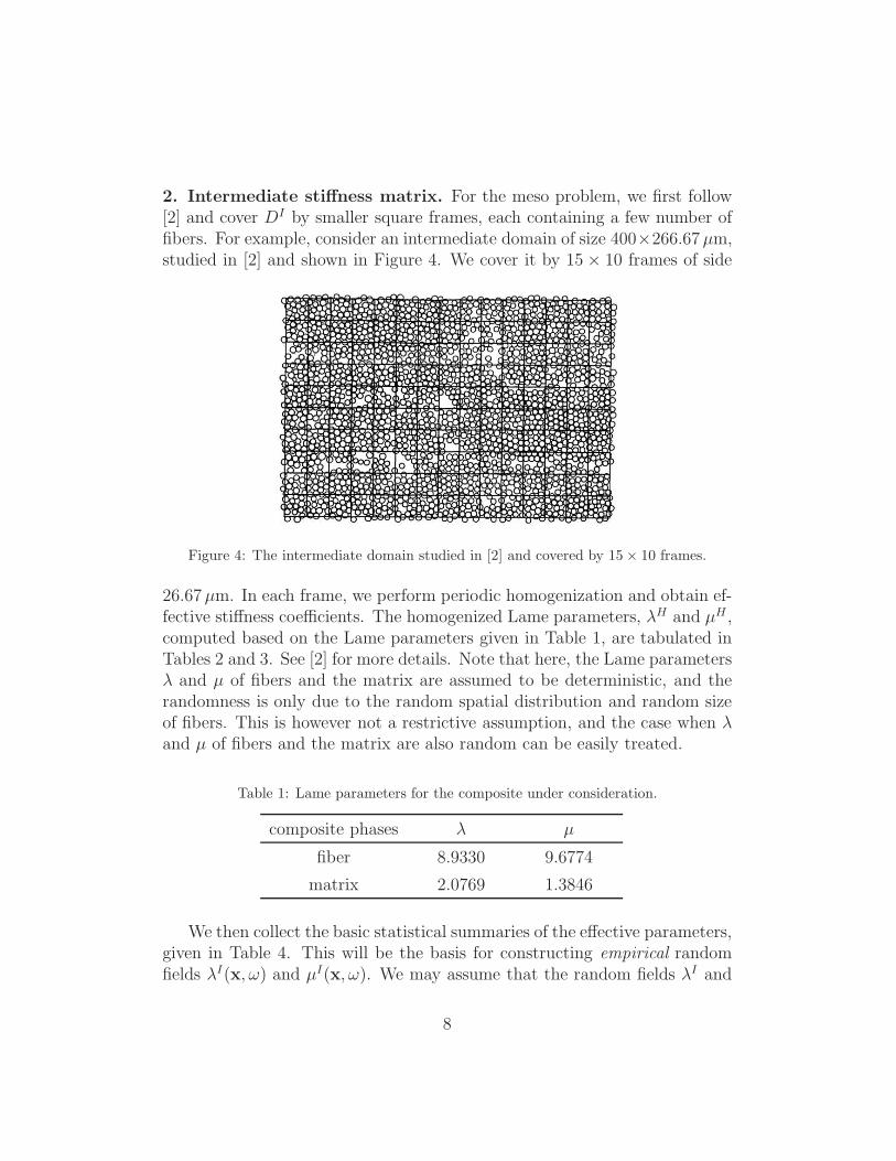
2. Intermediate stiffness matrix. For the meso problem, we first follow[2] and cover DI by smaller square frames, each containing a few number offibers. For example, consider an intermediate domain of size 400×266.67µm,studied in [2] and shown in Figure 4. We cover it by 15 × 10 frames of side

Figure 4: The intermediate domain studied in [2] and covered by 15× 10 frames.

26.67µm. In each frame, we perform periodic homogenization and obtain ef-fective stiffness coefficients. The homogenized Lame parameters, λH and µH ,computed based on the Lame parameters given in Table 1, are tabulated inTables 2 and 3. See [2] for more details. Note that here, the Lame parametersλ and µ of fibers and the matrix are assumed to be deterministic, and therandomness is only due to the random spatial distribution and random sizeof fibers. This is however not a restrictive assumption, and the case when λand µ of fibers and the matrix are also random can be easily treated.

Table 1: Lame parameters for the composite under consideration.

composite phases λ µ

fiber 8.9330 9.6774

matrix 2.0769 1.3846

We then collect the basic statistical summaries of the effective parameters,given in Table 4. This will be the basis for constructing empirical randomfields λI(x, ω) and µI(x, ω). We may assume that the random fields λI and

8

Table 2: Effective Lame’s first parameter λH from the 15× 10 grid shown in Figure 4.

4.9 3.4 4.2 3.7 4.2 5.1 3.7 4.4 3.6 4.0 3.4 2.6 3.1 4.1 4.03.4 3.7 4.8 4.2 4.6 4.4 4.2 4.9 2.1 3.0 3.4 4.9 4.3 3.3 3.73.1 3.6 4.2 4.5 4.7 4.2 4.5 3.2 4.5 2.6 4.5 4.0 4.1 4.8 3.33.4 3.2 4.2 4.5 3.9 3.2 4.8 4.3 4.9 3.8 3.8 3.5 3.4 3.9 3.34.8 4.4 2.7 3.5 3.2 3.8 3.6 3.3 4.5 3.5 4.8 3.7 3.1 3.0 5.14.5 3.2 4.3 3.5 4.7 3.8 2.4 4.0 3.6 5.5 4.3 4.1 4.9 3.6 4.03.4 4.3 4.0 3.8 2.3 3.9 3.8 2.6 4.0 4.7 5.2 3.9 4.9 4.0 4.25.2 4.8 3.7 3.1 4.2 2.3 4.4 5.7 4.0 4.2 3.6 4.2 4.2 4.7 3.93.2 3.9 4.4 5.0 2.6 4.7 3.3 5.1 3.8 3.9 3.6 4.1 3.3 3.8 4.94.0 3.3 3.6 3.9 4.2 3.8 4.2 3.2 4.0 3.0 3.9 3.2 4.5 4.2 3.3

Table 3: Effective Lame’s second parameter µH from the 15× 10 grid shown in Figure 4.

4.6 4.2 4.5 4.4 4.0 4.1 3.9 4.0 2.6 3.2 3.5 3.4 3.9 4.2 3.53.8 4.2 4.5 4.3 4.6 4.5 4.2 4.4 2.4 2.5 4.1 4.8 4.2 3.1 3.32.7 2.5 3.4 3.9 3.8 3.4 3.5 2.7 3.2 1.8 3.9 3.8 4.1 3.9 3.34.0 3.5 4.1 3.9 4.1 3.8 4.5 4.0 4.6 3.0 4.3 4.1 3.7 4.2 3.34.4 4.1 3.3 2.6 2.8 3.0 3.9 2.8 3.8 2.8 4.8 3.9 4.1 3.3 3.93.9 3.5 4.4 3.8 4.6 3.8 4.0 3.4 3.9 4.5 4.1 4.9 5.0 3.6 4.33.6 4.0 5.1 3.7 3.6 3.8 4.6 2.9 4.0 4.7 4.8 4.3 4.8 4.0 4.84.3 3.7 2.3 2.2 2.9 2.1 3.7 3.6 3.3 3.2 2.6 2.7 3.3 3.1 3.33.9 4.3 4.7 4.5 3.6 4.2 4.7 4.3 3.4 3.8 3.3 4.5 3.3 3.6 4.34.2 3.9 4.9 4.5 3.7 3.7 4.5 3.8 3.9 2.9 3.6 3.7 4.3 4.6 4.4

µI have a stationary Gaussian covariance structure. We then obtain theirspatial correlation lengths, say Lc, from the homogenized data λH and µH ,see e.g. [19]. Moreover, the statistical analysis in [2] suggests that the randomfields λI and µI may also be cross-correlated with a cross correlation matrix

Ccross =

[

1 cc 1

]

. (3)

We then perform a truncated Karhunen-Loeve decomposition of cross-correlatednormal random fields [20] and obtain the effective random fields Gλ(x, Y

Iλ )

and Gµ(x, YIµ ), where Y I = [Y I

λ , YIµ ] is a random vector of N I independent

normal random variables. The number of modes N I in the Karhunen-Loeve

9

Table 4: Statistical summaries of the effective homogenized Lame parameters for the15× 10 grid shown in Figure 4.

Statistic λH µH

Min 2.1 1.8

Max 5.8 5.1

Mean 3.9 3.7

S.D. 0.7 0.7

expansion is chosen such that a high percentage of the standard deviationis preserved. Finally, in order for the empirical random fields λI and µI tohave correct marginal distributions, we let each random field have a betadistribution with four parameters: the exponents α and β, and the minimumand the maximum of the distribution range a and b. These four parametersare computed so that the statistic measures in Table 4 are satisfied. Forexample, let Fλ and Fµ be the resulting cumulative distribution functionscorresponding to the statistical summaries of λH and µH , respectively. Therandom fields λI and µI are then given by

λI(x, Y Iλ ) = F−1

λ Φ(Gλ(x, YIλ )), µI(x, Y I

µ ) = F−1µ Φ(Gµ(x, Y

Iµ )),

where Φ is the normal cumulative distribution function. The stiffness matrixfor the meso problem CI = CI(x, Y I) is therefore obtained in terms of therandom vector Y I = [Y I

λ , YIµ ] consisting of N I independent normal random

variables.3. Global stiffness matrix. The effective global stiffness matrix CG inD is a constant and deterministic matrix obtained either by putting straingages on the side of the laminate, or by employing stochastic homogeniza-tion techniques under proper stationarity and ergodicity assumptions on therandom fields obtained in the meso level. See [9, 10, 7] for further details onstochastic homogenization.

After computing stiffness matrices for the three problems, in the last stepof the algorithm, we solve the following three problems simultaneously:

10

I. Micro problem. The main problem we want to solve is the micro problemin the local domain DL,

(x, Y L)utt(t,x, Y )−∇ · σ(u(t,x, Y )) = f in [0, T ]×DL × Γ, (4a)

u(0,x, Y ) = g1(x), ut(0,x, Y ) = g2(x) on t = 0 ×DL × Γ, (4b)

u(t,x, Y ) = gI(t,x, Y I) on [0, T ]× ∂DL × Γ. (4c)

The random vector Y = [Y L, Y I ] has in total N = NL + N I independentrandom variables YnNn=1. We denote by Γn ≡ Yn(Ω) the image of Yn and letΓ =

∏Nn=1 Γn. We further assume that the random vector Y ∈ Γ ⊂ RN has

a bounded joint probability density function ρ : Γ → R+ with ρ ∈ L∞(Γ).The random density (x, Y L) and stiffness matrix CL(x, Y L) are directlyobtained from the fiber positions and diameters, as described above. We usethe stochastic collocation method (see Section 3.3) to compute the statisticalmoments of given quantities of interest. The boundary force term gI(t,x, Y I)on ∂DL is obtained from the intermediate solution uI to the following mesoproblem (see Section 3.2).II. Meso problem. At each collocation point obtained in the micro prob-lem, we solve the following problem in the intermediate domain DI ,

(x, Y I)utt(t,x, YI)−∇ · σ(u(t,x, Y I)) = f in [0, T ]×DI × ΓI , (5a)

u(0,x, Y I) = g1(x), ut(0,x, YI) = g2(x) on t = 0 ×DI × ΓI , (5b)

u(t,x, Y I) = gG(t,x) on [0, T ]× ∂DI × ΓI , (5c)

where the random density (x, Y I) and stiffness matrix CI(x, Y I) are ob-tained based on N I independent Gaussian random variables, as describedabove, and ΓI =

∏Nn=NL+1 Γn. The boundary force term gG(t,x) on ∂DI is

obtained from the global solution uG to the following macro problem.III. Macro problem. The global solution uG is obtained by solving thedeterministic macro problem (1) in D where the random density and stiff-ness matrix C are replaced with the effective deterministic constant densityρG and constant stiffness matrix CG. We use a deterministic solver such asthe finite difference or the finite element method.

3.2. Computation of internal boundary conditions

Suppose that a two-dimensional local domain of interest DL ⊂ DI isgiven. The exact Dirichlet boundary condition on the boundary ∂DL reads

u∣

∣

∂DL = g∗(t,x, Y I), ∀x ∈ ∂DL.

11

For every fixed Y I ∈ ΓI , we can approximate the function g∗ by the value ofthe intermediate solution uI on ∂DL:

g∗(t,x, Y I) ≈ uI(t,x, Y I)∣

∣

∂DL =: gI . (6)

A simple way to do this is to compute uI and its spatial derivatives ∂x1uI and

∂x2uI at the center xc of the domain DL and then apply Taylor expansion

around this point. We obtain for every x ∈ ∂DL,

uIi

∣

∣

∂DL ≈ uIi

∣

∣

xc+ (x− xc)

⊤∇uIi

∣

∣

xc, i = 1, 2. (7)

In a similar way, we can obtain the boundary condition for the intermediateproblem.

Remark 2. It is well known that this approximation introduces the so-calledpollution effects [24, 28]. One way to reduce the error is to consider a largerdomain containingDL. We can further improve the accuracy of (6) by addingcorrection terms. We write

g∗ ≈ gI = (g1, g2)⊤, gi = uI

i

∣

∣

∂DL +ϕ⊤∇uI

i

∣

∣

∂DL , i = 1, 2. (8)

Here, uIi and ∇uI

i on ∂DL are computed from (7). Moreover, to compute ϕ,we first notice that the solution on the boundary given in (8) needs to satisfythe PDE in the micro problem. This gives a PDE for ϕ. We augment thePDE with periodic boundary conditions.

3.3. Stochastic collocation method

In this section, we briefly review the stochastic collocation method forcomputing the statistical moments of the solution to the micro problem (4),where Y ∈ Γ ⊂ RN is a vector of N independent random variables [5, 29, 22].

The stochastic collocation method consists of three main steps. First,the problem (4) is discretized in space and time, using a deterministic nu-merical method, such as the finite element or the finite difference method.We denote the semi-discrete solution by uh(t,x, Y ), where h represents thediscretization mesh size and time step. The obtained semi-discrete problemis then collocated in a set of η collocation points Y (k)ηk=1 ∈ Γ to com-pute the approximate solutions uh(t,x, Y

(k)). Finally, a global polynomialapproximation uh,p is built upon those evaluations

uh,p(t,x, Y ) =

η∑

k=1

uh(t,x, Y(k))Lk(Y ),

12

for suitable multivariate polynomials Lkηk=1 such as Lagrange polynomials.Here, p represents the polynomial degree.

A key point in the stochastic collocation method is the choice of the setof collocation points Y (k), i.e. the type of computational grid in the N -dimensional stochastic space. A full tensor grid, based on cartesian productof mono-dimensional grids, can only be used when the number of stochasticdimensions N is small, since the computational cost grows exponentially fastwith N (curse of dimensionality).

Alternatively, sparse grids can reduce the curse of dimensionality. Theywere originally introduced by Smolyak for high dimensional quadrature andinterpolation computations [25]. Two typical examples of sparse grids includetotal degree and hyperbolic cross sparse grids. We refer to [5, 29, 22] for moredetails.

The ultimate goal of the computations is the prediction of statisticalmoments of some given quantities of interest Q(u). The quantity of interestmay be either a function, e.g. the solution u, or a functional of the solution,e.g. the spatial and temporal averages of the solution, or an operator appliedto the solution, e.g. the components of the stress tensor. Using the Gaussquadrature formula for approximating integrals, we write

E [Q(u(., Y ))] ≈ E [Q(uh(., Y ))] =

∫

Γ

Q(uh(., Y )) ρ(Y ) dY

≈η(ℓ)∑

k=1

θk Q(uh(., Y(k))) =: Eℓ[Q(uh(., Y ))].

The weights are

θk =

N∏

n=1

∫

Γn

Lkn(Yn) ρn(Yn) dYn, Lkn(Yn) =

η∏

i=0, i 6=kn

Yn − Y(i)n

Y(kn)n − Y

(i)n

,

and the collocation points Y (k) = [Y(k1)1 , . . . , Y

(kN )N ] ∈ Γ are tensorized Gauss

points with Y(kn)n , kn = 0, 1, . . . , pn, being the zeros of the ρn-orthogonal

polynomial of degree pn +1. Here, for any vector of indices [k1, . . . , kN ] with0 ≤ kn ≤ pn the associated global index reads k = 1+k1+(p1+1) k2+(p1+1) (p2+1) k3 + . . . . The positive integer ℓ is called the level, and pn(ℓ) is themaximum degree of polynomials in the n-th direction, with n = 1, . . . , N ,given as a function of the level ℓ.

13

3.4. Stochastic regularity of quantities of interest

The convergence rate of error in the stochastic collocation method de-pends on the regularity of the quantity of interest Q(uh) with respect tothe random input variable Y . This regularity is called stochastic regularity,which is in turn related to the regularity of the coefficients and data in thephysical space. A fast/exponential convergence is obtained in the presenceof high stochastic regularity or stochastic analyticity.

Recently, it is shown in [22, 21] that the solution of stochastic hyperbolicproblems, unlike the solution of elliptic and parabolic problems, is not ingeneral analytic with respect to the random variables. The wave solutionsmay posses high regularity for particular types of smooth data. However,in real applications, the data are not smooth. Therefore, the convergencerate of error in the wave solution may only be algebraic. Yet, a fast spectralconvergence is possible for mollified quantities of interest.

Following [21], we propose to perform a low-pass filtering (moving aver-age) in order to isolate and remove the non-physical oscillations in Q(uh),which are a result of its low regularity. This is done by convolving the oscil-latory quantity of interest with a Gaussian kernel

Kδ(x) =1

2 π δ2exp

(

−|x|22 δ2

)

, (9)

with the standard deviation δ. See Remark 3 for more comments on δ. Thefiltered quantity is then given by

Qδ(uh)(t,x, Y ) = (Q(uh) ⋆ Kδ)(t,x, Y ) =

∫

DL

Kδ(x− x)Q(uh)(t, x, Y ) dx.

(10)We note that due to the boundary effects introduced by the convolution,we compute the filtered quantity on a smaller domain x ∈ Dδ ⊂ DL withdist(∂Dδ, ∂D

L) ≥ d > 0. We choose d so that Kδ(x0) with |x0| = d isessentially zero. This implies that for any x ∈ Dδ, the support of Kδ(x− x)is essentially vanishing at ∂DL. A practical choice is for example d ≥ 2 δ.

Remark 3. There are two different motivations for performing a low-pass fil-ter; physical and numerical ones. The physical motivation arises for instancein seismology, where the simulated seismic data are often post-processed byperforming a low-pass filter in order to isolate and remove the high-frequency

14

modes. An example is when high-frequency modes do not excite a given in-frastructure and are therefore removed. The numerical motivation arises forinstance due to the presence of high-frequency modes which are not resolvedon the spatial mesh. In this case, the generated high-frequency noise in thesolution is filtered out for accuracy reasons. Another example is when werequire higher regularity in the solution with respect to a given input param-eter, which is obtained by performing a low-pass filter. We note that whenthe filtered solution is a physical quantity, the standard deviation δ is a givenconstant. In fact, in the example mentioned here, δ is inversely proportionalto the maximum frequency that is allowed to pass. On the other hand, whena low-pass filter is performed for numerical purposes, an error is introduced,which depends on δ. In this case, the value of δ is selected so that the totalerror does not exceed a given tolerance TOL. See Section 4.5 for more details.

4. Error analysis

In this section, we present a simple error analysis to give a qualitativeinsight into different sources of errors in the presented algorithm. We studythe effect of different parameters and factors on the error. The results willbe supported by the numerical experiments in the next section.

We consider the micro problem (4) in the local domain DL, with

σ(u) = λ(x, Y L)∇ · u I + µ(x, Y L) (∇u+∇u⊤).

The random parameters , λ, and µ are directly obtained from the fiberlocations and diameters. The random boundary data gI in (4c) is numericallycomputed and is only an approximation of the true boundary data g∗. Weassume that u∗ is the exact solution to the micro problem (4) with the trueboundary data g∗. The ultimate goal of computations is to approximatestatistical moments of a quantity of interest Q(u∗) inside the local domain.For instance, assume that the quantity of interest is a bounded operatorapplied to the solution, e.g. a component of the stress tensor in the localdomain DL, and that we want to compute its expected value E[Q(u∗)]. LetEℓ[Qδ(uh)] be the approximation to E[Q(u∗)], obtained by the algorithmdescribed in Section 3. The total error then reads

ε := ||E[Q(u∗)]− Eℓ[Qδ(uh)] ||, (11)

where || . || denotes the L2(0, T ;L2(DL)) norm. Note that if the quantity ofinterest is a functional on the solution, e.g. a spatial and temporal average

15

of the solution over the local domain DL, then the norm || . || will simplychange to the absolute value.

One can distinguish four different types of errors in the approximation:

1. Error in the calculation of boundary data gI for the local problem.

2. Spatial and temporal discretization error in the deterministic solver.

3. Filtering error.

4. Error in the stochastic collocation method.

Accordingly, we split the total error into four parts and write

ε ≤ εI + εII + εIII + εIV , (12)

where

εI = ||E[Q(u∗)]− E[Q(u)] ||, (13a)

εII = ||E[Q(u)]− E[Q(uh)] ||, (13b)

εIII = ||E[Q(uh)]− E[Qδ(uh)] ||, (13c)

εIV = ||E[Qδ(uh)]− Eℓ[Qδ(uh)] ||. (13d)

We will consider and discuss each error separately.

4.1. Error in boundary data

We first note that due to the well-posedness of the local stochastic IBVP(4), there exists a unique weak solution that depends continuously on thedata, see [21]. Consequently, we have for every Y ∈ Γ,

||u∗ − u||L2(0,T,H1(DL)) ≤ C ||g∗ − gI ||L2(0,T,H1/2(∂DL)).

The magnitude of the first error εI is therefore controlled by the error in theapproximation of the true boundary data g∗.

Next, we note that the error in the boundary data is due to two differentsources:

(i) Error due to the pollution effect (discussed in Section 3.2).

(ii) Errors in the computation of the intermediate solution uI , which is inturn due to

16

– Error in the approximation of the effective stiffness matrix in themeso problem CI , including the homogenization error and thetruncation error in K-L representation.

– Spatial and temporal discretization error in the meso problem.

– Error in the calculation of the boundary data gG for the interme-diate problem.

Let C∗I be the true stiffness matrix in the meso problem. It is well knownthat due to the continuous dependence of solution on the coefficients underproper regularity assumptions, one can bound the changes in the solution|u∗I − uI | by the changes in the coefficients |C∗I −CI |, see e.g. [11, 26]. Forexample, in [26], it is shown that if an expansion of the CI coefficients isconvergent, then the corresponding solutions will converge to the solution ofthe limiting system.

4.2. Discretization error in the deterministic solver

The discretization error εII in (12) represents the convergence of the de-terministic numerical scheme with respect to the mesh size h in the microproblem. With a uniform mesh, we have

εII = O(hr), r ≥ 1,

where r is the minimum between the order of accuracy of the finite elementor finite difference method used and the regularity of the solution. We notethat both spatial mesh sizes ∆x1 and ∆x2 and time step ∆t are of order hand related by a proper CFL condition. Also Note that the constant in theterm O(hr) depends on Q(uh) and is uniform with respect to Y , see [22].

4.3. Filtering error

Consider a scalar function Q ∈ C∞(R2). Let Qδ(x) := (Q⋆Kδ)(x) be thefiltered function, where the kernel and convolutions are defined in (9) and(10). We use the change of variables

x− x

δ= z,

and write

Qδ(x) =

∫

DL

Kδ(x− x)Q(x) dx =1

2 π

∫

DL

e−|z|2/2Q(x− δ z) dz.

17

The Taylor expansion of Q(x− δ z) around x gives

Qδ(x) =1

2 π

∫

DL

e−|z|2/2(

Q(x)− δ z⊤ ∇Q(x) +δ2

2z⊤ D2Q(x) z+O(δ3)

)

dz,

where, D2 is the Hessian matrix. We note that∫

e−z2i /2 zpi dzi =

Cp, p even,0, p odd,

i = 1, 2,

with Cp being a constant. We then obtain

|Q(x)−Qδ(x)| ∝ δ2 |D2Q(x)|,

where the size of the coefficient |D2Q(x)| depends on the spatial regularityof Q. For instance, when Q = Q(uh) ∈ H1(DL), by the inverse inequality,provided a uniform mesh is used in the deterministic solver, we have

||∂xi xjQ(uh)||L2(DL) ≤ Cinv h

−1||Q(uh)||H1(DL).

Therefore, we obtain the upper error bound

εIII ≤ O(δ2 h−1).

As mentioned in Remark 3, the parameters δ and h are chosen so that thetotal error does not exceed a given TOL. See Section 4.5 for more details.

4.4. Error in the stochastic collocation method

As extensively discussed in [22, 21], the error in the stochastic collocationmethod εIV is related to the stochastic regularity of the quantity of interest.

For simplicity, we consider the quantity of interest Q(u) = u and inves-tigate the stochastic regularity of Qδ(uh) = Kδ ⋆ uh. There are two sourcesof regularity in both spatial and stochastic spaces: the spatial discretization;and the filtering.

We first study the regularity due to the spatial discretization. By em-ploying the inverse inequality, we write for a multi-index k ∈ Z2

+,

||∂k

xuh||L2(DL) ≤ Cinv h

−|k| ||uh||L2(DL).

Through the Stochastic PDE, the spatial regularity can be transformed intothe regularity in the stochastic space, see Theorem 6 of [22]. We have

||∂k

Y uh||L2(DL) ≤ |k|!C |k| ||uh||L2(DL), C = O(h−1).

18

Consequently, for every Y ∈ Γ the power series uh : CN → L∞(0, T ;H10(D))

defined by

uh(t,x, Z) =∞∑

k=0

∑

|k|=k

(Z − Y )k

k!∂k

Y uh(t,x, Y ),

with k! = ΠNn=1(kn!) and Y k = ΠN

n=1Yknn converges for all Z ∈ CN such that

|Zn − Yn| ≤ τ = O(h). By a continuation argument, the function uh cananalytically be extended on the whole region

Σ(Γ, τ) = Z ∈ CN , dist(Γn, Zn) ≤ τ = O(h), n = 1, . . . , N.

Notice that the radius of the Y -analyticity is τ = τh = O(h).We next study the regularity due to the Gaussian filtering. Due to the

separability of the two-dimensional Gaussian kernel Kδ, the spatial deriva-tive of the kernel can be constructed as the product of two one-dimensionalGaussian derivative functions. We then have

∂k

xKδ(x) = (

−1√2 δ

)|k|Hk1(x1√2 δ

)Hk2(x2√2 δ

)Kδ(x),

where Hk is a Hermite polynomial of degree k. Hence,

∂k

xQδ(uh) =

∫

DL

∂k

xKδ(x− x)Q(uh)(t, x, Y ) dx = O(δ−2 |k|).

As before, the spatial regularity is transformed into the stochastic regularity,and we have

||∂k

YQδ(uh)||L2(DL) ≤ C |k| ||Qδ(uh)||L2(DL), C = O(δ−2).

Hence, the radius of the Y -analyticity is τ = τδ = O(δ2).It is shown in [22] that the interpolation error in the stochastic collo-

cation for a quantity of interest with the radius of Y -analyticity τ is pro-portional to e−c τ ℓ, where c > 0 is a bounded constant. For example, usingan isotropic sparse tensor product interpolation based on Gauss-Legandreabscissas, where ℓ ≥ c0/ logN , with c0 > 0 being a constant, we obtain

εIV ≤ O(η−c1 δ2/ logN).

Moreover, for any quantity of interest with s bounded mixed Y -derivatives,the interpolation error is shown to be proportional to η−c2 s/ logN , where c2 > 0is a bounded constant [22]. Therefore, we have

εIV ≤ min(

O(η−c1 δ2/ logN),O(η−c2 s/ logN))

. (14)

19

Remark 4. As a simple example, consider the Cauchy problem for the one-dimensional acoustic wave equation

utt(t, x, y)− y2 uxx = 0 in [0, T ]× R× Ω,

u(0, x, y) = g(x), ut(0, x, y) = 0 on t = 0 × R× Ω,

By the d’Alembert’s formula, the solution reads

u(t, x, y) =1

2[g(x− y t) + g(x+ y t)].

Now, since

∂xu =1

2[g′(x− y t) + g′(x+ y t)], ∂yu =

1

2[−t g′(x− y t) + t g′(x+ y t)],

the spatial and stochastic regularity of the solution u are both related to theregularity of g and hence related.

4.5. Computational cost versus error minimization

There are three main parameters, (h, δ, η(ℓ)), that control the computa-tional cost W and the error E := εII+εIII+εIV . In order to find the optimalchoice of the parameters, we need to minimize the computational complexityof the stochastic collocation method, subject to the total error constraintE = TOL. We first note that

Eℓ[Qδ(uh)] = Eℓ[Kδ ⋆Q(uh)] = Kδ ⋆ Eℓ[Q(uh)]. (16)

The computational cost of the second term in (16) is of order η (δ−d+h−(d+1)),while the cost for computing the last term is of order δ−d + η h−(d+1), whered is the spatial dimension (here d = 2). It is therefore more economical toemploy the last expression in (16) for computing Eℓ[Qδ(uh)]. Therefore

W ∝ δ−d + η h−(d+1). (17)

Moreover, from the previous sections, we have for an isotropic sparse tensorproduct interpolation based on Gauss-Legandre abscissas,

E ∝ hr + δ2 h−1 + η−c δ2/ logN , (18)

under the assumption that εIV is bounded by the first term in (14).

20

We now introduce the Lagrange function

L := W + λ (E − TOL),

with the Lagrange multiplier λ. We note that in practice, the constants inthe error terms are important and need to be considered and included in theLagrange function. The optimal choice of the parameters are then obtainedby equating the partial derivatives of the Lagrange functions with respect tothe parameters h, δ, η, and λ to zero.

As an example, consider the case where δ is fixed. This occurs when forinstance the filtered quantity is a physical quantity of interest, see Remark3. Then the Lagrange function corresponding to (17) and (18) reads

L = η h−(d+1) + λ (hr + η−2/ logN − TOL).

The optimal choice of the parameter h is then obtained by

hr ≈ TOL/(

1 +r logN

s (d+ 1)

)

,

resulting in the computational work W ∝ TOL− logN/s−(d+1)/r.

5. Numerical experiments

In this section, we present several numerical examples to demonstrate theefficiency and applicability of the global-local algorithm described above.

We consider a ply of long unidirectional fibers with zero angle in the stateof plane strain in R3. The material is assumed to be isotropic. The governingequation is given by the stochastic PDE (1a) with the stress tensor (2). Weassume = 1, and let the materials properties, i.e. the Lame parametersλ and µ of fibers and the matrix, be deterministic and given by Table 1.We further assume that the randomness in the coefficients is only due to therandom spatial distribution and random size of fibers. The volume fractionof fibers is assumed to be 59%.

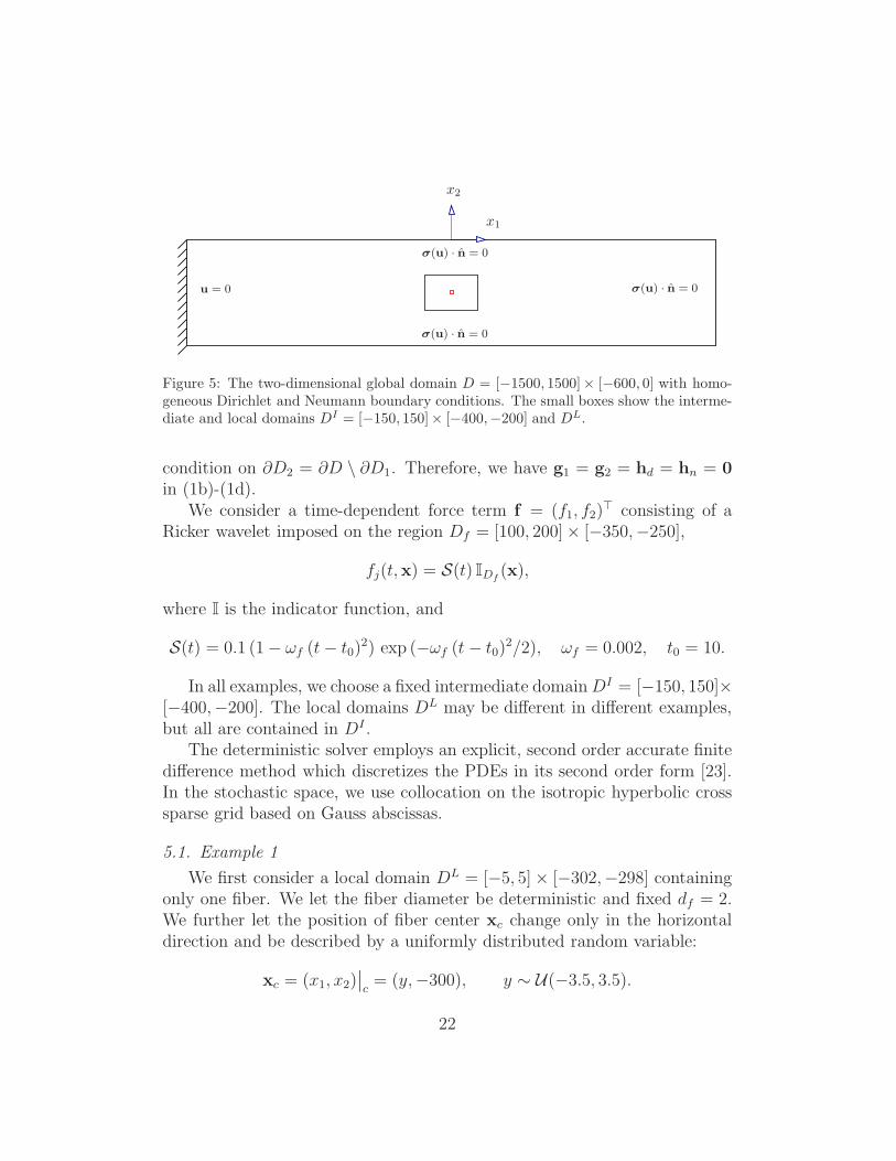
We let D = [−1500, 1500]× [−600, 0] be the two-dimensional global do-main, which is the orthogonal cross section of the ply, see Fig. 5. Weconsider homogeneous initial conditions and impose homogeneous Dirichlet(no displacement) boundary condition on the left boundary ∂D1 = x | x1 =−1500, x2 ∈ [−600, 0], and homogeneous Neumann (no traction) boundary

21

u = 0

σ(u) · n = 0

σ(u) · n = 0

σ(u) · n = 0

x1

x2

Figure 5: The two-dimensional global domain D = [−1500, 1500]× [−600, 0] with homo-geneous Dirichlet and Neumann boundary conditions. The small boxes show the interme-diate and local domains DI = [−150, 150]× [−400,−200] and DL.

condition on ∂D2 = ∂D \ ∂D1. Therefore, we have g1 = g2 = hd = hn = 0

in (1b)-(1d).We consider a time-dependent force term f = (f1, f2)

⊤ consisting of aRicker wavelet imposed on the region Df = [100, 200]× [−350,−250],

fj(t,x) = S(t) IDf(x),

where I is the indicator function, and

S(t) = 0.1 (1− ωf (t− t0)2) exp (−ωf (t− t0)

2/2), ωf = 0.002, t0 = 10.

In all examples, we choose a fixed intermediate domainDI = [−150, 150]×[−400,−200]. The local domains DL may be different in different examples,but all are contained in DI .

The deterministic solver employs an explicit, second order accurate finitedifference method which discretizes the PDEs in its second order form [23].In the stochastic space, we use collocation on the isotropic hyperbolic crosssparse grid based on Gauss abscissas.

5.1. Example 1

We first consider a local domain DL = [−5, 5]× [−302,−298] containingonly one fiber. We let the fiber diameter be deterministic and fixed df = 2.We further let the position of fiber center xc change only in the horizontaldirection and be described by a uniformly distributed random variable:

xc = (x1, x2)∣

∣

c= (y,−300), y ∼ U(−3.5, 3.5).

22

For the meso problem, we choose deterministic parameters λI = 3.9, andµI = 3.7, which are the mean values given in Table 4. We therefore haveonly one uniformly distributed random variable Y = y.

Finally, for the macro problem in the global domain D, we choose thefollowing deterministic effective parameters

λG = 0.59 λfiber + 0.41 λmatrix, µG = 0.59µfiber + 0.41µmatrix.

We consider the horizontal component of the normal stress as the quantityof interest

Q(u) = σx1(t,x, Y ).

We solve the problem using the multi-level algorithm and compute the ex-pected value of the quantity of interest

Qℓ,h(t,x) := Eℓ[Q(uh)](t,x) = Eℓ[σh x1](t,x), (19)

where the subscripts ℓ and h represent the level in the stochastic space andthe mesh size in the micro problem. Fig. 6 shows Qℓ,h at time t = 70and x ∈ D with the mesh size h = 0.125 and for four different levels ℓ =10, 20, 100, 10000.

We observe that for small values of ℓ, i.e. small number of collocationpoints, the quantity of interest Qℓ,h is oscillatory, and as ℓ increases theoscillations damp out, and we obtain a uniform solution which is expected.It is however very expensive to use a large number of collocation points,especially in high stochastic dimensions. As an alternative, we propose touse a low number of sample points, which is affordable, and then to performa low-pass filtering (10) on the oscillatory quantity of interest (19) using aGaussian kernel (9). Let Qℓ,h,δ := Eℓ[Qδ(uh)](t,x), where δ is the standarddeviation of the kernel. We let the non-filtered solution obtained by a largelevel ℓ∗ = 10000 be a reference solution and compute two relative errors:

E∞(t) :=||Qℓ∗,h(t, .)−Qℓ,h,δ(t, .)||L∞(Dδ)

||Qℓ∗,h(t, .)||L∞(Dδ)

,

E2(t) :=||Qℓ∗,h(t, .)−Qℓ,h,δ(t, .)||L2(Dδ)

||Qℓ∗,h(t, .)||L2(Dδ)

.

We set Dδ = [−4.25, 4.25]× [−301.25.− 298.75]. Table 5 shows the relativeerrors at time t=70 for different levels with a fixed h = 0.125. We have

23

−5 0 5−302

−301

−300

−299

−298

0.8

0.9

1

1.1

1.2

x1

x2

(a) ℓ = 10

−5 0 5−302

−301

−300

−299

−298

0.8

0.9

1

1.1

1.2

x1

x2

(b) ℓ = 20

−5 0 5−302

−301

−300

−299

−298

0.8

0.9

1

1.1

x1

x2

(c) ℓ = 100

−5 0 5−302

−301

−300

−299

−298

0.8

0.9

1

1.1

x1x2

(d) ℓ = 10000

Figure 6: The expected value of the stress Eℓ[σh x1](t,x) at time t = 70 and x ∈ DL, with

the mesh size h = 0.125 and for four different levels ℓ = 10, 20, 100, 10000.

Table 5: Relative errors in the filtered quantity of interest at time t=70.

levels δ E∞ E210 1.3 0.03 0.010

20 0.9 0.02 0.009

100 0.4 0.01 0.003

empirically observed that the choice δ = 4/√ℓ results in small relative errors.

Figure 7 shows the absolute value of the error |Qℓ∗,h(t, .)−Qℓ,h,δ(t, .)| inDδ ⊂ DL at time t=70 for the level ℓ = 20. Note that since the position ofthe fiber center changes only in the horizontal direction, we apply filteringonly on the horizontal direction in order to avoid introducing errors in thevertical direction, where there are no fibers in the region x2 ∈ [−302,−301]∪[−299,−298].

24

−5 0 5−302

−301

−300

−299

−298

0.005

0.01

0.015

0.02

0.025

x1

x2

Figure 7: The absolute value of the error |Qℓ∗,h(t, .) − Qℓ,h,δ(t, .)| in Dδ ⊂ DL at timet=70 for the level ℓ = 20 with ℓ∗ = 10000 and h = 0.125.

5.2. Example 2

We now consider a local domain DL = [−4, 4]× [−308,−292] containingtwo fibers with deterministic and fixed diameters df = 2, see Fig. 8. Wefurther divide the local domain into two equal parts and confine a fiber ineach part. This prevents the two fibers from intersecting each other. We letthe position of fiber centers change only in the horizontal direction and bedescribed by two independent uniform random variables:

(x1, x2)∣

∣

c1= (y1,−300), (x1, x2)

∣

∣

c2= (y2,−300),

wherey1 ∼ U(−2,−1.05), y2 ∼ U(1.05, 2).

This choice will allow the two fibers get very close to each other with aminimum distance of 0.1.

The material coefficients for the meso and macro problems are determin-istic and chosen as in Example 1. We therefore have two independent uniformrandom variables in total, and hence Y = (y1, y2)

⊤.Fig. 9 shows Qℓ,h in (19) at time t = 70 and x ∈ DL with the mesh

size h = 0.1 and for four different levels ℓ = 10, 20, 1000, 5000. As before,we observe non-physical oscillations for small values of ℓ, and as ℓ increasesthe oscillations damp out and we obtain a uniform solution as expected. Byconvolving the stress, obtained by a small level, with a Gaussian kernel, weagain obtain good results comparable to the non-filtered stress obtained bya large level.

25

F1 F2

c1 c2xr1

xr2

Figure 8: The two-dimensional local domain DL = [−4, 4]× [−302,−298] containing twofibers. The fiber diameters are fixed df = 2, and the position of fiber centers are modeledby uniform random variables.

−4 −2 0 2 4−302

−301

−300

−299

−298

2

3

4

5

6

x1

x2

(a) ℓ = 10

−4 −2 0 2 4−302

−301

−300

−299

−298

2

3

4

5

6

x1

x2

(b) ℓ = 20

−4 −2 0 2 4−302

−301

−300

−299

−298

2

3

4

5

6

x1

x2

(c) ℓ = 1000

−4 −2 0 2 4−302

−301

−300

−299

−298

2

3

4

5

6

x1

x2

(d) ℓ = 5000

Figure 9: The expected value of the stress Eℓ[σh x1](t,x) at time t = 70 and x ∈ DL with

the mesh size h = 0.1 and for four different levels ℓ = 10, 20, 1000, 5000.

We next compute the time-history of the expected values of the stress(19) at a point xr1 = (0,−300) between the two fibers. Fig. 10 shows themean plus and minus the standard deviation of the stress σx1 at point xr1 asa function of time.

We also compare the values of stress at two different points: between thetwo fibers at xr1 = (0,−300), and away from the fibers at xr2 = (−3,−301).Fig. 11 shows that the stress values between two fibers is larger than thestress values at a point away from the fibers. This is due to the fact that the

26

0 200 400 600 800 1,000−30

−20

−10

0

10

20

t

Qℓ,h

Qℓ,h

Qℓ,h ± SD

Figure 10: Mean (tick blue line), plus and minus the standard deviation (thin red line) ofthe stress σx1

at point xr1 as a function of time.

fibers can get very close to each other and this concentrates the stress.

0 200 400 600 800 1,000−20

−10

0

10

20

t

Qℓ,h

Qℓ,h(.,xr1)

Qℓ,h(.,xr2)

Figure 11: Mean of the stress σx1at two different points xr1 and xr2 as a function of time.

Due to the concentration of the stress between fibers, which may be very close to eachother, stress at xr1 is higher than stress at xr2 .

5.3. Example 3

We finally consider a local domain DL = [−4.5, 4.5] × [−302.5,−297.5]containing two fibers with variable diameters. Motivated by [2], we assumethat the fiber diameters have a truncated Gaussian distribution with a meanµd = 2µm and standard deviation σd = 0.18µm and a cut-off parametercd = 3. Therefore, if y is a random variable with a truncated normal densityfunction

ρd(y) =exp (−y2/2) I[−cd,cd]∫ cd−cd

exp (−z2/2) dz,

27

the fiber diameters dfj , j = 1, 2, read

dfj = µd + σd yj, yj ∼ Ncd(0, 1), j = 1, 2.

We further divide the local domain into two parts and confine one fiber ineach part, see Fig. 12. This prevents the two fibers from intersecting eachother. We let the position of fiber centers in both horizontal and verticaldirections be described by uniformly distributed random variables:

(x1, x2)∣

∣

c1= (y3, y4), (x1, x2)

∣

∣

c2= (y5, y6), yj ∼ U(aj , bj), j = 3, . . . , 6,

where (a3, b3) = (−2.3,−1.3), (a4, b4) = (a6, b6) = (−300.5,−299.5), and(a5, b5) = (1.3, 2.3).

F1

F2

c1

c2

Figure 12: The two-dimensional local domain DL = [−4.5, 4.5] × [−302.5,−297.5] con-taining two fibers. The fiber diameters and the position of fiber centers are modeled bytruncated Gaussian and uniform random variables, respectively.

The stiffness matrix for the micro problem CL = CL(x, Y L) is thereforeobtained in terms of the random vector Y L = [y1, . . . , y6]

⊤ consisting of sixindependent random variables with truncated Gaussian (two variables) anduniform (four variables) distributions.

For the meso problem in the intermediate domain DI = [−150, 150] ×[−400,−200], we use the effective stiffness coefficients obtained as describedin Section 3.1 with the correlation length Lc = 120 and the cross-corrolationmatrix (3) with c = 0.6. By choosing N I = 8 modes in the K-L expansion,80% of the standard deviation is preserved. The effective coefficients forthe meso problem is therefore obtained in terms of the random vector Y I =[Y I

λ , YIµ ] consisting of N I = 8 independent normal random variables. Hence,

the vector Y = [Y L, Y I ] contains N = NL + N I = 14 independent randomvariables.

28

The deterministic effective coefficients for the macro problem in the globaldomain D = [−1500, 1500]× [−600, 0], are choosen as in Example 1.

Fig. 13 shows Qℓ,h in (19) at time t = 70 and x ∈ DL with the meshsize h = 0.1 and for two different levels ℓ = 10, 30, with the number ofcollocation points η = 6077, 218767, respectively. As before, we observe non-

−4 −3 −2 −1 0 1 2 3 4

−302

−301

−300

−299

−298

−2

0

2

4

6

8

x1

x2

(a) ℓ = 10

−4 −3 −2 −1 0 1 2 3 4

−302

−301

−300

−299

−298

−2

0

2

4

6

8

x1x2

(b) ℓ = 30

Figure 13: The expected value of the stress Eℓ[σh x1](t,x) at time t = 70 and x ∈ DL with

the mesh size h = 0.1 and for two different levels ℓ = 10, 30.

physical oscillations for small values of ℓ. However, in this case, since thestochastic dimension is relatively large, N = 14, it is not practical to increaseℓ to a high level. As an alternative, we can convolve the solution obtainedwith a low level ℓ with a Gaussian kernel in order to remove the non-physicaloscillations. Fig. 14 shows the filtered quantity Qℓ,h,δ with ℓ = 10 and

δ = 4/√ℓ in Dδ ⊂ DL at time t=70 and with h = 0.1. To find a reference

−4 −3 −2 −1 0 1 2 3 4

−302

−301

−300

−299

−298

2.5

3

3.5

4

4.5

x1

x2

Figure 14: The expected value of the filtered stress Qℓ,h,δ with ℓ = 10 and δ = 4/√ℓ in

Dδ ⊂ DL at time t=70 and with h = 0.1.

solution, we employ the Monte Carlo method with NMC = 105 sampling

29

points in the stochastic space. Using the obtained reference solution, therelative errors in the filtered quantity Qℓ,h,δ with ℓ = 10 at time t = 70 areE∞ = 0.04 and E2 = 0.02.

6. Conclusions

We have proposed a stochastic multilevel global-local algorithm for solv-ing the elastodynamic equations in fiber-reinforced composite materials. Themethod aims at approximating statistical moments of some given quantitiesof interest, such as stresses, in regions of relatively small size. For a fiber-reinforced cross-plied laminate, we introduce three problems (macro, meso,micro) corresponding to the three present scales (laminate, ply, fiber). Thealgorithm uses the homogenized global solution to construct a good localapproximation that captures the microscale features of the real solution. Wehave presented a qualitative study on different sources of error in the algo-rithm. We have performed numerical experiments that show the applicabil-ity and efficiency of the method. We note that, to the best of the authors’knowledge, the inclusion and propagation of uncertainty in the elastodynamicmodel for fiber composites is not addressed in the literature, and what wepropose in the present work is the first numerical platform for treating suchproblems.

Future directions include performing a more rigorous error analysis, par-ticularly on the filtering error and interpolation error in the stochastic col-location method, and presenting an alternative numerical algorithm whichdoes not rely on the homogenized global solution. This is the subject of ourcurrent work and will be presented elsewhere.

Acknowledgements

The authors would like to recognize the support of the PECOS centerat ICES, University of Texas at Austin (Project Number 024550, Center forPredictive Computational Science). Support from the VR project ”Effektivanumeriska metoder for stokastiska differentialekvationer med tillampningar”and King Abdullah University of Science and Technology (KAUST) AEAproject ”Bayesian earthquake source validation for ground motion simula-tion” is also acknowledged. The second and third authors are members ofthe KAUST SRI Center for Uncertainty Quantification in ComputationalScience and Engineering.

30

References

[1] I. Babuska. Homogenization and its applications, mathematical andcomputational problems. In B. Hubbard, editor, Numerical Solutionsof Partial Differential Equations-III, (SYNSPADE 1975, College ParkMD, May 1975), pages 89–116, New York, 1976. Academic Press.

[2] I. Babuska, B. Andersson, P. J. Smith, and K. Levin. Damage analysisof fiber composites, Part I: statistical analysis on fiber scale. Comput.Methods Appl. Mech. Engrg., 172:27–77, 1999.

[3] I. Babuska, G. Galoz, and J. Osborn. Special finite element methods fora class of second order elliptic problems with rough coefficients. SIAMJ. Numer. Anal., 31:945–981, 1994.

[4] I. Babuska and R. Lipton. l2-global to local projection: an approachto multiscale analysis. Math. Mod. Methods Appl. Sci., 21:2211–2226,2011.

[5] I. Babuska, F. Nobile, and R. Tempone. A stochastic collocation methodfor elliptic partial differential equations with random input data. SIAMJ. Numer. Anal., 45:1005–1034, 2007.

[6] I. Babuska and J. E. Osborn. Generalized finite element methods: Theirperformance and their relation to the mixed methods. SIAM J. Numer.Anal., 20:510–536, 1983.

[7] G. Bal. Waves in random media. Lecture notes, Columbia University,NY, 2006.

[8] J. F. Bourgat. Numerical experiments of the homogenization methodfor operators with periodic coefficients, volume 707 of Lecture Notes inMathematics. Springer-Verlag, 1977.

[9] A. Bourgeat and A. Piatnitski. Approximation of effective coefficientsin stochastic homogenization. Ann. Inst. H. Poincare Prob. Statistics,40:153–165, 2004.

[10] J. Bystrom, J. Engstrom, and P. Wall. Periodic approximation of elasticproperties of random media. Advances in Algebra and Analysis, 1:103–113, 2006.

31

[11] J. Charrier. Strong and weak error estimates for elliptic partial dif-ferential equations with random coefficients. IMA J. Numer. Anal.,50:216–246, 2012.

[12] W. E and B. Engquist. The heterogeneous multiscale methods. Com-mun. Math. Sci., 1:87–132, 2003.

[13] W. E, B. Engquist, X. Li, W. Ren, and E. Vanden-Eijnden. Heteroge-neous multiscale methods: A review. Commun. Comput. Phys., 2:367–450, 2007.

[14] Y. Efendiev and T. Y. Hou. Multiscale finite element methods. Springer.

[15] B. Engquist, H. Holst, and O. Runborg. Multiscale methods for wavepropagation in heterogeneous media. Commun. Math. Sci., 9:33–56,2011.

[16] B. Engquist and P. E. Souganidis. Asymptotic and numerical homoge-nization. Acta Numer., 17:147–190, 2008.

[17] T. Y. Hou and X. Wu. A multiscale finite element method for ellipticproblems in composite materials and porous media. J. Comput. Phys.,134:169–189, 1997.

[18] T. J. R. Hughes, G. R. Feijoo, L. Mazzei, and J. B. Quincy. The vari-ational multiscale method. A paradigm for computationnal mechanics.Comput. Methods Appl. Mech. Engrg., 166:3–24, 1998.

[19] W. F. Krajewski and C. J. Duffy. Estimation of correlation structure fora homogeneous isotropic random field: A simulation study. Computers& Geosciences, 14:113–122, 1988.

[20] V. Miroslav. Simulation of simply cross correlated random fields byseries expansion methods. Structural Safety, 30:337–363, 2008.

[21] M. Motamed, F. Nobile, and R. Tempone. Analysis and computationof the elastic wave equation with random coefficients. IMA J. Numer.Anal., 2012. (under review).

[22] M. Motamed, F. Nobile, and R. Tempone. A stochastic collocationmethod for the second order wave equation with a discontinuous randomspeed. Numer. Math., 2012. (to appear).

32

[23] S. Nilsson, N. A. Petersson, B. Sjogren, and H.-O. Kreiss. Stable dif-ference approximations for the elastic wave equation in second orderformulation. SIAM J. Numer. Anal., 45:1902–1936, 2007.

[24] J. T. Oden and K. S. Vemaganti. Estimation of local modeling errorand goal-oriented adaptive modeling of heterogeneous materials. I: errorestimates and adaptive algorithms. J. Comput. Phys., 164:22–47, 2000.

[25] S. A. Smolyak. Quadrature and interpolation formulas for tensor prod-ucts of certain classes of functions. Doklady Akademii Nauk SSSR,4:240–243, 1963.

[26] C. C. Stolk. On the modeling and inversion of seismic data. PhD thesis,Utrecht University, The Netherlands, 2000.

[27] T. Strouboulis, I. Babuska, and K. Copps. The design and analysis ofthe generalized finite element method. Comput. Methods Appl. Mech.Engrg., 192:3109–3161, 2003.

[28] K. S. Vemaganti and J. T. Oden. Estimation of local modeling error andgoal-oriented adaptive modeling of heterogeneous materials. II: a com-putational environment for adaptive modeling of heterogeneous elasticsolids. Comput. Methods Appl. Mech. Engrg., 190:6089–6124, 2001.

[29] D. Xiu and J. S. Hesthaven. High-order collocation methods for differ-ential equations with random inputs. SIAM J. Sci. Comput., 27:1118–1139, 2005.

33