Six Sigma Prof. Dr. T.P.Bagchi Department of Management...

Six Sigma Prof. Dr. T.P.Bagchi

Department of Management Indian Institute of Technology, Kharagpur

Lecture No. # 19

Design of Sampling Plans

(Refer Slide Time: 00:28)

Good afternoon again. We ended the last session with the short view of the signal sample

plan. In fact that plan is still showing on the screen there, I take a lot of size big n as

sample n. I can sort of it, which is of what quality p, which is unknown quantity. And I

inspect all the items there and the number of defects turns out to be d. And then I

compare that number of items found defective that little d to be. I compare that to this

little control number called c. If d is less than or equal to c, I accept the lot, otherwise I

reject the lot. Now in doing that, if you remember I had it on my on my table here. And I

utilized what we called a little formula which came from the binomial distribution. Now,

I am going to actually give you this formula there, so that you will have a pretty descent

idea, how to utilize binomial distribution?


Now, if lot quantity, lot quality, if this is taken to be p that is p is the fraction defective in

the lot. Then suppose I picked n items the probability that I will pick, I will find d

defectives in n items that I pick out of this. When overall lot quality is p, this turns out to

be a binomial distribution. And that goes like this probability is equal to n choose d p to

the power d 1 minus p to the power n minus d.

And this formulas tells you that you know this is the exact formula that tells you. If n

items were chosen if their inspector and d defectives were found, where p is the overall

defect level of the lot Then this is the expression that will give you the quantity p

quantity p or P a or the probability of finding d defectives in n items. And here of course,

let us write the range of d, d can be as small as 0. It can be 1 2 and so on and it can be at

most be equal to n. This is the range of this, and this particular distribution is called the

binomial distribution. (No audio from 2:50 to3:03)

Couple of assumptions here, one is that n is very large, that is like one. It is a very big

assumption there, and sometimes lots are pretty big, in fact it turns out, if your sample

size and lot size if the ratio of if this little n is one tenth of this. You can apply this

formula there is no problem. There lots of sampling plans have been designed based on

this, and I am going to be showing a you use of this particular formula in designing a

single sample plan. I will do that.


Let us first take a look at something called the OC curve. The operating characteristic

curve of the plan. Now notice in the recall that, when I drew the single sampling plan and

I had this item there, I had this particular item there.


The quantity that I was most interested was this probability. The probability of accepting

the lot, that is what I had a lot of interest in this, because this is the probability of

accepting the lot which is at quality level p.

So, this is a very important quality. I really need to really have a good field for this.

Now, if p changes if little p changes P A also will change, because that will be

determined by this formula, there as I change P A is going to change. P A is the chance

of accepting the lot, the probability of accepting the lot. Now, there must be A between

this little p and P A, that is shown by the OC curve.


Let us take a look at this curve there. What is this curve called? The OC curve, it is the

graph of the percent defective p in a lot or batch verses the probability that the sampling

plan will accept the lot, which is P A. So in fact it is a plot between P a big P A and little

p. That is what this plot is. That is what the OC curve is. And this is determined on the is

all really dependent on the sampling plan. The particular sampling plan you are using

that is going to determine the duration ship between little p and P a.

In fact what you would like is, you would like this sampling plan in such a way, that this

P a is high. When your lot quality p is very near AQL, and also you would like this P a to

be small as small as possible when this lot quality is near or QL. These are the two kind

of relation that you must have, in fact the more the plan is able to reject lots at the RQL

level to more discriminating it is.

It should accept most of the lots which are at AQL level; it should reject lots which are

generally around RQL level .Then I will say it is a good plan, now to get an idea whether

the plan is good or bad. We need to look at the OC curve of the plan and I am going to

show you, what that OC curve really shows you?


Here is the picture of the OC curve of a typical sampling plan. Let us look at the axis

first, on the x axis I have got lot quality which is little p, little p is on the x axis, and on

the y axis I have got P a, P a is the probability of accepting the lot that, is big P a big P a

goes this way.

Now, notice something I would like I as a user of this sampling plan. I would like to

have when my lot quality is near AQL. And let us pretend here that AQL is three

percent, if AQL is three percent, I would like to have a high P a at this point. I would like

to have a high P a and the curve shows here that this particular some sampling plan from

which this plot has been drawn. It will accept ninety percent of the lots which are

submitted with your little p at 3 percent level. Now, the same plan will accept a very

small number only ten percent of the lots. When your lot quality little p becomes ten

percent so like if RQL is 10 percent, then only ten percent of the lots would be accepted

by the sampling plan.

Now, what happens in between you see this slopping curve, there is a formula for it. I am

going to show you, what that formula is like? That formula gives you for any value of p,

it will give you the corresponding value of P A. So what does the OC curve show you?

What does it show you? It shows you the chance of accepting a lot at the RQL level. It is

also showing you the chance of rejecting a lot.

When the lot really is at the AQL level and it also shows you the fat of all the lots.

Which are at quality levels? Which are between AQL and RQL? That is what the OC

curve does? So the OC curve actually it is a pretty useful piece of curve, it is a pretty

useful device. And this can be drawn exactly, and I am going to show you the method for

drawing this exactly.


So, again let us come back and look at some of the terms there. Acceptable qualitable

level is the percent of defectives that the customer is willing to live with forever.

Because that level of defect in the incoming lots is a with him, then there is of course,

this other idea called LTPD or RQL. It is the upper limit on the percent of defects that

the customer is willing to accept, but only with a very small probability.

Then, there is some other term called AOQ average outgoing quality. I am going to show

you what that quantity is and of course, there is a limit on that AOQ also which is called

AOQL. And that also, I am going to show you what these are? So, in fact we know what

AQL is? We know what LTPD or RQL is? They are the same terms. And I am going to

explain to you what AOQ is and what AOQL?


These I am going to show to you now, what about an ideal curve? Ideally speaking of

course, you would like to reject as many lots at the near the RQL level as possible. You

would like to reject as many lots as possible which are near, which are at quality level.

That is near RQL and you would like to accept any lot that is coming at or better than

what we call the AQL level. So in fact at AQL level my P A. P A is the probability of

accepting it should be very close to one and at RQL level, my probability of accepting

should be very close to 0 this is the ideal curve.

Now, think for a minute I could have a sampling plan that will operate actually in this

ideal mode, provided I did 100 percent inspection. And I made no inspection errors I

committed no inspection errors. If I was able to do that, I will be able to operate pretty

comfortably. Because I will be accepting all the lots which are acceptable and I will be

rejecting all the lots which are, which should be rejected that I should be able to do.


But what happens in real life? In real life I am not doing 100 percent inspection. So my

real plan is going to be either like, this is the real OC curve of a plan that I have used or it

could be like this, the black curve there. So, either the red curve or the black curve, this

is what reality is going to be. Like what is the difference between these two? It turns out

that the black curve will throw away, will reject most of the lots that are at poor quality

level. It will accept almost all the lots which are at AQL level, AQL being 3 percent and

RQL being around here. It will reject most of the lots which are in this area.

Now, look at the red curve, this is another sampling plan. It is got the OC curve of that

plan, there the red one. It is not as discriminating; it is not able to separate between good

and bad lots as effectively as the black curve. In fact the ideal plan would be like you go

down just a little bit, then you come all the way vertically down. Then you go out this

way that was the ideal curve. And the black curve approaches it, so the black curve is

better than the black sampling plan is better than the red dotted sampling plan.


Now, what are the things that are of interested the producer? The producer would like to

make sure that the sampling plan accepts as many lots as possible which are submitted at

the AQL level. And what is it that the consumers would like to do? The consumer would

like to have the sampling plan reject as many lots as possible, which arrive at RQL level.

Now, once you set up your sampling procedure, you basically take these rules and you

give the gauge. You give the gauge to the inspector, and you tell him now you operate

any lots that are arriving by trucks boxes and so on and so forth.

You utilize my sampling rule and my sampling rule is what? Pick little n items and I am

also going to give you this control number c. Look up the number of defectives found in

those n items, if the number of defectives found exceeds c. Reject the lot, if the number

of defectives found in the little n items which were inspected. Because now, this is the

sample and you must inspect every item in the sample. If that number d is less than or

equal to c accept the lot, this is from my production, this is who you would like to do,

you able to do.

Obviously, the producer would like you to accept as many lots as possible. You would

like to you, they would like to make sure that your P a at the AQL level should be pretty

close to one. And the consumers would like to make sure that the P a at the RQL level is

as close to 0 as possible. This is like something that is desired by the two parties which

are forming the two ends of the supply chain.


So, in fact in general look at alpha and look at beta now, beta is the probability of my of

my accepting a lot which is at LTPD or RQL level. Beta is the chance of the sampling

plan accepting a lot which is at RQL or LTPD level. That suppose to be quite small it is

kept generally around not more than ten percent. And alpha is the chance of my rejecting

a lot which is like 1 minus P a at this point 1 minus P a at this point. That is equal to

alpha that is the probability of my rejecting a lot which is otherwise at AQL level.

At this level, ideally I should be accepting all the lots. But I reject alpha fraction of the

lots, this alpha and this beta, these are the contention these are actually the ones that we

have to balance.


So, there are these two types of risks involved wrongful rejection and the fraction of

items fraction of lots that are rejected at the AQL level. That is equal to alpha and

wrongful acceptance of poor lots. Poor lots are of quality RQL that quantity is suppose to

be beta. I should not exceed alpha in rejecting good lots and I should not exceed beta in

accepting what we call bad lots? Which are bad lots are near RQL level.


And, a curve like this is not very discriminating; it will probably allow a lot of bad lots.

Also to come in to the system, the ideal curve is like this, which you know stays near one

near AQL and falls to the ground. And, it rejects every lot that is slightly different from

your AQL level. Therefore, there is actually there is some reason for us to take plans

which are here. And to try to make sure that these plans are approach this ideal plot, this

is what we would like to be able to do so? We would like to design sampling plan, this is

like a particular sampling plan.

This is not very discriminating, what we would like to be able to do is? We would like to

design a sampling plan in such a way, that this plan is as close to this ideal shape as

possible.


Let us see, how we do that? This is again a continuation of the same thing bad lots

differently at this end, and good lots are at this end. That is what they are in between of

course. There are lots that will be accepted, because I am not doing 100 percent

inspection. And I would like to make sure that this curve approaches the ideal curve as

much as possible; this is what I would like to be able to do?


Now, there are ways to calculate these numbers, there are ways to calculate these

different numbers. And those would be using the remember the binomial formula that I

had there. The binomial formula is shown here, this is the binomial formula, this P a

equal to summation d equal to 0 to c n choose d p to the power d 1 minus p to the power

n minus d. This is the formula that gives me P a and with the help of this by plugging in

different values of p I can determine the values of P a Q. And I can produce a plot; the

plot looks like the plot that I have got on the screen here. This plot can be plotted once I

have my binomial formula with me.


Now, some times what happens? That the lots supplied is of finite size like for example,

a truck or a bus. In that case we use a distribution that is the hyper geometric distribution

not the binomial distribution. We use the binomial distribution when the lot size is so

large, then it can pretend that big n is too large. When I compare that to little n and I can

use the binomial distribution, I should be able to use this binomial distribution which is

here. When lot size is quiet large, but if lot size itself that big n there, if this big n is not

too large, I have to use what we call the hyper geometric distribution? And in that case, I

will be using the type A OC curves.


It is also possible for me instead of using the binomial distribution. I may be able to use

the Poisson distribution also and the formula is shown here. P r is now the probability.


And I am going to be drawing that for you, P r is the probability. And if I draw it

correctly using the Poisson distribution, the Poisson formula goes like this. First of all

there being r defectives, this is equal to n p raise to the power r e minus n p divide by r

factorial. This is the formula for finding exactly r defectives, when I sample from an item

which is got n and p is the overall quality of that lot. There n items have been sampled

from it in which r defectives have been found, p is the overall quality of the lot that is

supplying those parts there.

Now, what have I got there couple of things are happened here. One is I made a decision,

Now I made a decision here to select a sample size of n. So sample size is n and lot

quality is p, these two are given to me. If these two are given to me then the Poisson

formula gives me the chance of finding r defects in n items. Chosen, this is a formula

which I can also use in designing a sampling plan or in fact in constructing the P A. The

P A number, the P A formula, how will I find P A? Suppose my rule is that you accept

the lot. P A is the probability of my finding d less than or equal to c. If I use the Poisson

formula this will turn out to be d equal to 0 to c n p to the power d divided by d factorial

e minus n p. This is the formula I will be using if I have to construct an OC curve that

uses the Poisson formula as the basis.

Now, this is an alternative to the binomial distribution. So, in fact there are several ways

I could construct this OC curve. I could use the binomial distribution which is this

formula, remember this formula. There, this is the binomial distribution or I could use

the Poisson distribution I could use the Poisson distribution whichever is convenient for

me.


If I doing the calculation, I could use that and by chance if it turns out that my sample

size is, what it is suppose to be, which is little n but my lot size is finite, my lot size is my

n, n is my lot size. And this n is not too large in that case I will be using the hyper

geometric distribution. And there, the formula is given by this and again I can work out

the exact formula for P a. The probability of accepting the lot, now this again is given in

your slides. As we go down you will be able to see this one and we will come back and

we will use this in a couple of minutes, we will be using this.


Let us carry on with our distribution. There, we were using the Poisson distribution, so

we got the Poisson formula there and with Poisson formula I can actually work out my P

a.


P a, remember P a is the y axis .P a turns out to y axis in the OC curve and the x axis in

that case turns out to be a little lot quality p lot. Quality p is here and P a is there and

when they end up with for a given n and a given value of p. I end up with the OC curve

there, what does the OC curve tell us? It tells us the risk of accepting a bad lot or the risk

of rejecting a good lot. Rejecting as a good lot is something that the supplier is going to

be upset with and accepting a bad lot is something that the user is going to be upset with.

And both of these we have to balance both of these, we have to minimize and generally

speaking the considerations are economic.


Like, I said to you earlier, we need not always worry about the binomial distribution. As

the only way we may be able to use the hyper geometric formula.


Or we may be able to utilize the binomial formula also. Hyper geometric Poisson or

binomial, these are three popular formulas which are utilized, in trying to draw the OC

curve in most cases.


The ideal OC curve of course, is like this. It just starts out; it accepts everything that is

near AQL; and it rejects everything that is beyond AQL; and this would be this situation;

I can guarantee this, provided I take the full lot. And inspect each and every item, I take

the full lot and I inspect every item. So, that I can pull out any defectives that might be

there, I pull out all the defectives and I end up with only good parts there. If I would do

that, I could operate in a way that would be pretty close to what we call the ideal curve

that we could do.


Now, the let us see how we balance the two risks. Now AQL is something that the

supplier knows, AQL is something that the consumer is willing to live with forever and

ever. And, therefore, the consumer is interested in making sure that he gets generally

items which are near AQL level. Occasionally, if he does get something that is near the

RQL level, the consumer would like to make sure that lots coming at near the RQL level.

Those are rejected, the producer on the other hand, he also knows that AQL is a quality

level that is acceptable to the consumer, to the user or the consumer. Therefore, what the

producer would like to make sure is that any lot that is submitted at AQL level of overall

quality, it is accepted by the customer.

Now, the decision to accept or reject the lot; that is based on the n c sampling plan that I

have in the single sampling case; therefore, we got to make sure when we design a

sampling plan, we do it in such a way that we take care of the interest of the of the user

and also the interest of the supplier. Both of those interests they have to be brought

together and there is a easy way to do this. Say, it is surprisingly easy they might appear

to be conflicting. But I will show you a process by which you will really see, it is not that

difficult to work this out.


This is of course, the binomial formula and it is just showing you that if you use the

binomial formula. You can construct the OC curve by changing the value of p, given a

value of n and given a value of c. If you change the little value of this, little p there you

can determine different values of P a. That will be generated from this and then you can

plot p verses P a, which is actually the trace of the OC curve itself. For any n for any

sample size and any control number c that is given to you.


So, in fact it is the same manner in which this OC curve has been generated. It is not very

difficult to do.


And of course, the ideal curve also I showed you the ideal curve is valid only when you

are doing a 100 percent inspection. It is not valid, otherwise that is something we would

like to be able to do.


Now, you know there are curves; there are various types of curve possible. Let me draw

a few curves here for you. I am going to be using this paper here.


And I am going to be drawing the two axis there, one axis is p is the overall quality and

this side I have got P A. P is the chance of accepting the lot the ideal curve of course, is it

is going to start at 1.0 and it is going to come down to RQL, AQL level and from that

point on it is going to stay right there near 0. And all the way beyond this RQL is here

this is like a an ideal OC curve but generally what happens here? OC curve. They behave

like this in other curve they may, it may behave like this a third curve, it may behave like

this.

Now, obviously look at these curves a little carefully, look at the value of beta. Let us

say RQL is here, beta here is quiet small. But beta here is somewhat larger and the beta

for this curve is quiet large now. What is beta provides the user or the consumer of the

protection? Say if large beta is there, the consumer is not going to be protected very well.

And you look at alpha, now alpha is small here. Alpha is protection provided to the

supplier, then I have got alpha here, which is slightly larger. And this one has got the

largest alpha, the larger is the alpha, the larger is the suppliers risk or the producers risk.

So in fact what the producer would like to do is? He would like to have as small as far as

possible alpha be small. This is what the producer would like to be able to do? And what

is it that the consumer would like? The consumer would like beta to be small, this is

what the user would like to be able to do or the producer would like to be able to do there

is the consumer would like to do.

So, the consumer looks at this end and the producer looks at this end. What we would

like to be able to do is? We would like set some target. Here I would like to set some

target here, and I would like to see can we construct a curve that goes through these two

points? This point and this point, can we do that this is something that we would like to

attempt.


Now, let us go to the screen, there notice here. What happens if I vary this curves, if I

change n, if I change n little n is the sample size. As sample size is increased, the OC

curve becomes more and more discriminating. So, it moves this way which is like it,

becomes better and better from the perspective of here. We have got RQL and the guy

who is most concerned with this is the consumer. So, it is better for the consumer to take

a large sample, remember this now it is better for the consumer to use large sample in

sampling.


And, now what about the other story? There, if I increase my c, the curve turns to rise

and when the curve rises, what happens to alpha? Look at what happens to alpha,

becomes smaller and smaller. When alpha become smaller, the producers risk goes down

the producers risk was high here. It became quiet small; there on the other hand the

consumers risk was low. Here low here and it got to a point which is like more than 0

definitely.

So, in fact, what we have to do is? We have to find a compromise between sample size

and this control number c in such a way that I am able to provide a protection to here.

The supplier or the producer and the consumer, who is the user of these items which are

arriving by lots.


Let us see, how we do that? We have some general definitions here; in fact these again

define AQL and RQL for us? AQL I have put in green and RQL or LTPD I have put in

red here.


And, these are two curves, now they are both actually for finite size lots. They are both

for finite size lots, if I look at infinite size lots, which happen sometimes when the supply

is such that the truck size is very large. And I have got continuous production feeding,

my factory continuous production by the supplier feeding my factory. Then of course,

the suppliers lot size is very large and I could be using the type B curve there. Now,

these are only to indicate to you that as far as large lots are concerned, there is not that

much difference in the OC curve.


Let us, take a look at, whether we use the Poisson distribution or some other distribution.

If lot size is large use the binomial distribution or the Poisson distribution. If lot size is

small use the binomial distribution, use the hyper geometric distribution. And let us try

to do a small problem; let us try to work out a very, very small problem, pretty simple

problem there. And what we would like to do is you see the problem that is indicated

right at the bottom. A lot of 20 tires containing 5 defective items, 5 defective would lead

to basically p being 25 percent defective, those are supplied to you.

If an inspector, randomly samples 4 items out of the 20 tires. What is the probability of

finding three defective ones? This exercise basically is a direct application of this

formula, there the hyper geometric formula. Let us see, how we do that?


I am going to be doing this; I am looking for the probability of three defectives. So I will

write this p three defectives and these three defectives are in four items. This should be

equal to now, look at the formula, out look at the formula given there, n minus r divided

by n minus r. Choose n minus m, let us try to write that. Here the first thing I would like

to do is, I would like to make sure that, I account for the number of items which are

picked out of the lot.

The lot size here is 20, so I put 20 there and sample size is 5 sample size in this case is 4

items only. So 4 is there, now this is the total number of combinations. Different number

of ways I could construct samples of size four picking out of 20 items, 20 items are the

basically the size of the lot.

Now, let us take a look at the number of defectives in the original lot which consist of 20

tires. There are 5 defective tires and I would like to have 3 defective tires appear in the

hands of the inspector. So 5, choose 3 is the number of different ways 3 defectives could

be picked out of 5 defectives, which are present in the lot itself.

Then, what about the items which are not defective? Those are 20 minus 5 and that is

equal to fifteen. And then what is the remaining number, it turns out that if I pick 4 items

if I pick 4 tires and 3 are defective. There is only going to be one that is going to be one

good one. This is the probability, now of my finding 3 defective tires, when I choose 4

tires out of lot of 20 which is got a total of 5 defective items in that. This has been done

using the hyper geometric distribution and this is a very important formula which we use.

Whenever we have got finite size lots, would like to use the hyper geometric distribution.


Let us, get back to the curves here, again these are couple of other curves that I show

here, to give you an idea that OC curves are never the same. OC curves depend a lot on

whether the lot is finite or the lot is infinite size. And, also if there are items which are

like the number of defectives that I allow to be in the lot. In the sample, which is the

control number c, if c changes the OC curve will change. If lot size changes big n

changes the curves will change the OC curve will change. And of course, if sample size

n changes little n changes then again the OC curves will change.

So, the OC curves dependent on all of these properties and of course, the OC curves tell

us whether a plan that I make my plan is always going to be an n c plan. Remember,

basically any kind of plan that I workout, whether it is a single sampling plan or a double

sampling plan. Anytime I have got a plan worked out that plan is going to be searched,

that I end up with protection provided to the user. And also it protect the supplier, the

user should not end up with a lot of defectives items. And supplier should not end up

with a lot of lots returned to him, which are otherwise at AQL quality level or near AQL

quality level. To do that we obviously have to optimally design the sampling plan.


This is like one other item that I should mention to you, might reject the lot. What is very

possible when you reject the lot? You would not want to return it to the supplier, what

you would like to do is? You would like to probably charge in for the defective items,

what you would like to sort the lot by doing 100 percent inspection. Remove the

defective items and make sure you can carry on with your production, because your

stoppage of production can be more expensive than returning the lot, and getting

replacement and so on and so forth. So what you would like to do most of the time is?

you would like to do rectification.

You look at the defective lots, once that are been rejected by your inspection procedure,

by your acceptance sampling procedure. And sort out the good items from the bad items.

Take the bad items; replace them with good items, now you got supplies now that can

carry through your production. So actually now you have got parts that you can carry,

that you can utilize in your production process. Mean while of course, you will negotiate

the deal with your supplier, as to what to do with the defective parts. Should he get more

replacement or should he charge him for some inspection cost and so on and so forth.

Those things you sort out separately, that you do when you are doing this? You would be

doing either, you would be doing rectified inspection or you would be doing just

standard rejection of the lot and returning the lot to the supplier.


Now, there is something that is also of interest to us. This is something that we would

like to call the AQL. AQL leading up to what we call AOQ? Now, suppose there is an

inspection plan in effect. What I have here, I have got an inspection plan that is in effect.


And, I have here, I am going to be doing that using a piece of paper, there my incoming

parts, those are coming in lot size of N is the lot size of an incoming parts. That is the lot

size and it is coming in at a quality level p 0. There is a certain probability of accepting

this lot and that probability is P A P A at p 0 level. And there is a certain chance of my

rejecting that lot and that is 1 minus P A is the probability of my rejecting the lot, how

many items are here?

Now, let us take a look accepted lots, those are accepted at probability P A. And, they are

of quality p 0, and the size is n. If you look at the number of items that comedown this

way, and if I actually workout the fraction of items the number of items which are

defective items in this strain. Let us see how we work it out on this side, on the average if

n items came in and I inspected them, I have N times P A. That is a chance of my going

this way and that is got a lot quality of p 0.

Now, look at this side, I have here lots coming in, they are getting rejected. And, they are

of course, all of them, they have been rectified. So, any items coming this way must all

be 100 percent on this side. Unfortunately I have drawn a sample, I have drawn a sample

and I have looked at the sample, and I have replaced any defective item that I have found

in the sample. Therefore, what I have here? If you look at the quantity here, I have the

average quality that is going out this way that if I indicate by this quantity called AOQ.

Average outgoing quality this way, that is going to be P A multiplied by big N minus n

multiplied by p 0 divided by N. Let me explain to you, what is going on here? N is the

total number of parts going through the system, once I have done rectification. I am not

returning anything to the supplier .So, the rejected lots they got rectified, they came

along I end up with some items here. And I end up with some items here. But the total

number of items coming this way is going to be N items.

Now, the once that have been accepted those are not been rectified on this strain .On this

side I have removed all the defective items but on this side I did my sampling. And, I

accepted them. Now, if there were any defectives in the little n samples, I remove those

defective items .And, I therefore, those n times p 0 those quantities have been removed.

So, the actual number of defectives going this way is going to be big N times p 0

multiplied by P A minus N times p 0 multiplied by P A. This is the number of defectives

that I let go this way. Therefore, the fraction that actually comes out as the result of

doing all this AOQ. AOQ at the outgoing level, this is at the average outgoing quality

living the inspection, both this area. This quantity turns out to be this quantity there.


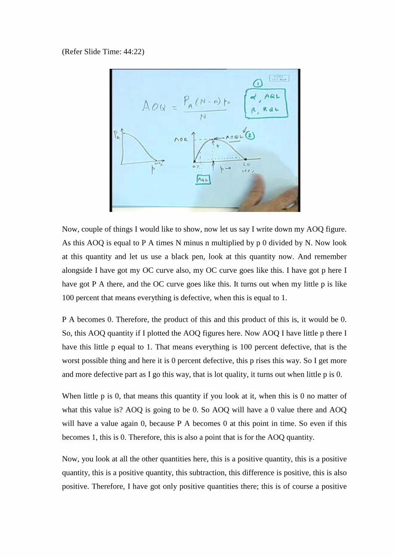
Now, couple of things I would like to show, now let us say I write down my AOQ figure.

As this AOQ is equal to P A times N minus n multiplied by p 0 divided by N. Now look

at this quantity and let us use a black pen, look at this quantity now. And remember

alongside I have got my OC curve also, my OC curve goes like this. I have got p here I

have got P A there, and the OC curve goes like this. It turns out when my little p is like

100 percent that means everything is defective, when this is equal to 1.

P A becomes 0. Therefore, the product of this and this product of this is, it would be 0.

So, this AOQ quantity if I plotted the AOQ figures here. Now AOQ I have little p there I

have this little p equal to 1. That means everything is 100 percent defective, that is the

worst possible thing and here it is 0 percent defective, this p rises this way. So I get more

and more defective part as I go this way, that is lot quality, it turns out when little p is 0.

When little p is 0, that means this quantity if you look at it, when this is 0 no matter of

what this value is? AOQ is going to be 0. So AOQ will have a 0 value there and AOQ

will have a value again 0, because P A becomes 0 at this point in time. So even if this

becomes 1, this is 0. Therefore, this is also a point that is for the AOQ quantity.

Now, you look at all the other quantities here, this is a positive quantity, this is a positive

quantity, this is a positive quantity, this subtraction, this difference is positive, this is also

positive. Therefore, I have got only positive quantities there; this is of course a positive

quantity. So, this curve between these two extremes must have some positive value, there

this is positive which actually says that if I am using the rectification scheme.

If I am using the rectification scheme at some point, I will have the worst level of defects

being passed. And this quantity, it can be this quantity, it can be determined. And also

this quantity can be determined. Now, sometimes what happens? The consumers would

like to tell you that there is a limit beyond which I cannot accept any kind of defects in

the lots, there is a limit there and this limit here is called AOQL, Average outgoing

quality limit. So, no matter of what inspection scheme? I am using AOQL actually tells

you the worst performance.

The worst performance of that sampling plan and many times consumers would like to

specify this to you, instead of giving you the, what we call the AQL? Remember AQL

was there, AQL you might think, that the consumer would be quite happy saying this to

you. But the problem is sometimes, we are also accepting lots which are at these quality

levels. And because of that the consumer comes along, he says I am going to give you a

quantity called AOQL. And please do not exceed that, no matter of what you do.

Therefore, this is like another criterion by which I could design my sampling plans. I

could of course, use the, I could use these things. I could use alpha AQL beta RQL, I

could use these constraints, I could use these constraints to design my sampling plan.

And, the other so this should be like one way. The other way would be to specify AOQL

and then come up with the plan.

I am going to show you a method that uses this technique. I am going to show you that,

these are the same calculations which are just shown here in different schemes.


And, here is an example of AOQL and this AOQL was specified by the consumer. And

therefore, he gets now 8.2 percent defectives in his items. That is the worst quality level,

he is going to experience if the same sampling plan is applied again and again .And here

again is the display of AOQL.


And, these curves can be drawn quiet easily. Because I remember, I have the formula; I

have this formula here with me. And I have this OC curve with me and with that I can

calculate the different point on this. And I can determine what that AOQL quantity is?

That is quite easy to determine.


And of course, double sampling plan would be an extension of what we have done so far.

I take an initial sample and I use the initial sample to come up with one kind of decision.

I may be able to accept the lot, I may be able to reject the lot .And I may not be able to

do that when I do double sampling. What I do is take a second sample, so I have taken a

first sample. But it did not lead to a decision; I was stuck between these two decision

points. Then I take a second sample and based on the result of the first sample plus the

second sample I may decide to accept the lot or to reject the lot.

This should be the way to do your double sampling plan. What the double sampling plan

does beyond the single sampling plan is? The double sampling plan generally gives you

a total lower on the average, it gives you fewer items to sample, that is one of the

advantages I am using the double sampling plan.


So, it gives you generally speaking a total, a smaller total number of items. I could

generalize that I could go to multiple sampling plans, where the rules become slightly

more complicated. But the follow essential the same procedure take one sample, check it

out. If the number of defectives found in that sample is between the limits where you

cannot really decide, you have to take on to another sample so on and so forth. You keep

doing this, you take the first sample, second sample, third sample and so on at some

point in time, you are going to make a decision either to accept it or to reject it.

Now, this may seem to be a little complicated to you, it turns out. To implement these

plans is somewhat of a complexity, because many times these procedures, they are not

clearly understood. By they can understand and they can many of them they follow the

single sampling plan without any trouble at all. But the movement you bring in more

stages of sampling, you go to the double sampling plan, the multiple sampling plan and

so on. Then it does become a bit complicated to implement on the floor, but what you

gain is? You have to do much fewer. You have got to do far fewer inspections, that is

what you should be able to do?


Then, there is something beyond this which is called the sequential sampling plan. And, I

am going to kind of just give you a hint of it there, what we do is? Instead of taking like

one lot of sample, which is like maybe of first sample will consist of these items? And

then the second sample will consist of some more items. There you put them all together,

that is your second item, second sample. I have got my first sample, and then I have got

my second sample and so on.

Then I tried to decide something on the basis of that the sequential sampling plans does.

Then something different, it again works with the same lot; the lot has been supplied to

you. What you do is you pick one item out of the lot and you take a look at it, do the

inspection and record it as good or bad. Then you take a second item; make sure the

record is kept there. Take the second item out and inspect it, to inspect, to see, if it is

good or bad. You do that.

Then, you take the third item again, you are, so what you are doing is? You are doing

one item at a time. You looked at the first item, you looked at the second item, you

looked at the third item, and you looked at the fourth item and so on. You keep going

like this, till at some point, you have to make a decision you end up with a decision and

that goes like this.


If I show you a curve there it will be not easier to see. Notice, here on the x axis I have

got the number of items sampled on the y axis. I have plotted here the number of

defectives found in this sequential sampling plan. You start with one item and you

basically, you got two control limits here .One is the acceptance control limit and this is

like a straight line, which is been drawn here, as a curvy stepwise kind of progress there.

I am going to show you, the other one also in a minute.

And, then I am going to get a rejection line also, if the trace of your sampling and results

of the sampling, if this stay within these two limits. You continue to sample, the moment

it goes either this way or this way, you decide to either accept the lot or to reject the lot.


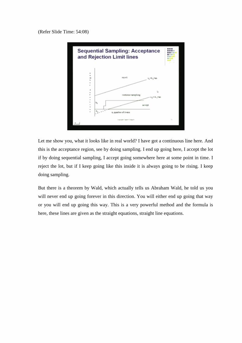
Let me show you, what it looks like in real world? I have got a continuous line here. And

this is the acceptance region, see by doing sampling. I end up going here, I accept the lot

if by doing sequential sampling, I accept going somewhere here at some point in time. I

reject the lot, but if I keep going like this inside it is always going to be rising. I keep

doing sampling.

But there is a theorem by Wald, which actually tells us Abraham Wald, he told us you

will never end up going forever in this direction. You will either end up going that way

or you will end up going this way. This is a very powerful method and the formula is

here, these lines are given as the straight equations, straight line equations.


And there parameters are given by this expression. Here, you got a rejection line which is

the lower line in the plot. And you got an acceptance line which is the upper line in the

plot. So, if we go back to the line. There this is the acceptance line on this region. In this

area you will accept, you end up coming here like this point. Here you will accept the lot

and if you end up going there, if you go end up going here. You will end up rejecting the

lot those are determined by this. And of course, the parameters to go into this equation,

those are given here by k 1 h 1 s 1 and h 2, what is the advantage in doing?


This is the first thing is the OC curves turn out to be very similar to what we done before.

But the beauty is that you end up with for fewer items to sample. When you do one item

at a time, when you keep picking one at a time. Your decision is reached much earlier,

because this is a sequential likelihood, this is a sequential likelihood of finding so many

defectives in a sequence. And that is a something that is got much more power,

something like that you could quiet easily do and we will follow through. Now, with the

design of the actual sampling plans and I will be showing you a couple of methods there.

Thank you very much.

Six Sigma Prof. Dr. T.P.Bagchi Department of Management...

Documents

Transcript of Six Sigma Prof. Dr. T.P.Bagchi Department of Management...