SINGLE-BOLTED CONNECTIONS FOR ORTHOTROPIC · PDF fileORTHOTROPIC FIBRE-REINFORCED COMPOSITE...

SINGLE-BOLTED CONNECTIONS FOR ORTHOTROPIC FIBRE-REINFORCED

COMPOSITE STRUCTURAL MEMBERS

BY

CHARLES N. ROSNER

A Thesis Submitted to the Faculty of Graduate Studies

in Partial Fulfilment of the Requirements for the Degree of

MASTER OF SCIENCE

Department of Civil Engineering University of Manitoba

Winnipeg, Manitoba

(c) September, 1992

THE UNIVERSITY OF MANITOBA

FACULTY OF GRADUATE STUDIES

The undersigned certify that they have read a Master's

. . . . . . . . . . . . . . . . . . . . . . . . . . . . . . . . . . . . . . . . . . . . . . . . . . . . . . .

. . . . . . . . . , . . . . . . . . . . . . . . . . . . . . . . . . . . . . . . . . . . . . . . . . . . . . . S b . tt d b Charles Rosner u m.l e y .......................................... .

in partial fulfillment of the requirements for the degree

of M. Sc. . . . . . . . . . . . . . . . . . . . . . . . . . . . . . . . . . . . . . . . . . . . . . . . . . . . . . . . The Thesis Examining committee certifies that the thesis

(and the oral examination, if required) is:

Approved x Not Approved

.~fld!J .. a dAdvisor

~.:??1~ A •

.1 I .~ ::''''~ • ••• •• I ..... " ... ~~J .•....•..•

. . . . . . . . . . . . . . . . . . . . . . . . . . .

. . . . . . . . . . . . . . . . . . . . . . . . . . . External Examiner

(Dr. L. Ayari, Mechanical Engng.)

~ ~ ~,2'1 ~ it 1 Date. · 1-0' l.f. ~ · ~ · .1. · · · .1. ~. '-.-:-.

ABSTRACT

Although the high strength-to-weight ratio makes fibre-reinforced composite

materials extremely attractive to the structural engineer, there is a lack of research,

and consequently, a lack of criteria needed to design structures, especially

connections, using these materials. The design of bolted connections for orthotropic

fibre-reinforced composite materials requires much more attention in comparison

to the connections used for standard isotropic homogenous structural steels. In light

of this, an experimental investigation was conducted at the University of Manitoba

to study the behaviour of connections fabricated from a glass-fibre-reinforced

composite material. A total of 102 single-bolt double-shear lap connections was

tested. The effects of the various geometric parameters including, the connection

width, edge distance, material thickness, and fibre orientation were studied. Based

on the research findings a design procedure is introduced which accounts for

material orthotropy, pseudo-yielding capability, and other factors that influence the

connection behaviour. The experimental results were used to correlate and refine

a proposed analytical model introduced to descnbe the behaviour of single-bolted

connections in composite materials. The proposed design procedure is capable of

predicting the ultimate load and failure modes of a connection with any geometry.

Because of the generic nature of the model, the design guidelines can be applied to

a multitude of composite material systems. Due to the model's simplicity, the

proposed design procedure is ideal for future design codes.

iii

ACKNOWLEDGEMENTS

The author wishes to express his sincere thanks to Dr. Sami Rizkalla for his

guidance and support throughout this investigation. His encouragement and

enthusiasm was nothing less than inspirational.

The author also wishes to express his appreciation for the technical assistance

of Ed Lemke, Moray McVey, and Marty Green, as well as the contributions of the

rest of the technical staff at the Structural Engineering and Construction Research

and Development Centre at the Un~versity of Manitoba.

The financial assistance of NSERC (National Science and Engineering

Research Council of Canada) is greatly appreciated.

Appreciation if also given to the faculty and graduate students of the Civil

Engineering Department for their help and suggestions.

Special thanks go to Khaled Soudki, who endured the graduate program along

with myself and who was always there to help.

Finally, the patience and support of my parents, family and friends cannot be

praised enough. For their encouragement, I am indebted.

iv

TABLE OF CONTENTS

ABSTRACT . . . . . . . . . . . . . . . . . . . . . . . . . . . . . . . . . . . . . . . . . . . . . .. iii

ACKNOWLEDGEMENTS ................. . . . . . . . . . . . . . . . . . .. iv

TABLE OF CONTEN1S ...................................... v

LIST OF TABLES ......................................... V1ll

LIST OF FIGURES ......................................... ix

CHAPTER 1 INTRODUCTION ................................ 1

1.1 GENERAL . . . . . . . . . . . . . . . . . . . . . . . . . . . . . . . . . . . . . . . .. 1

1.2 OBJECTIVE ....................................... 3

1.3 SCOPE . . . . . . . . . . . . . . . . . . . . . . . . . . . . . . . . . . . . . . . . . . .. 3

CHAPTER 2 LITERATURE REVIEW . . . . . . . . . . . . . . . . . . . . . . . . . .. 4

2.1 INTRODUCTION TO COMPOSITES .................... 4

2.2 BOLTED CONNECTIONS IN COMPOSITE MATERIALS .... 7

2.3 FAILURE MODES .................................. 9

2.4 EXPERIMENTAL RESEARCH ......................... 9

2.4.1 Single-Bolt Connections ......................... 9

2.4.2 Multi-Bolt Connections . . . . . . . . . . . . . . . . . . . . . . . .. 12

2.4.3 Environmental Effects . . . . . . . . . . . . . . . . . . . . . . . . .. 14

2.4.4 Design Considerations. . . . . . . . . . . . . . . . . . . . . . . . .. 16

2.5 ANALYTICAL RESEARCH .......................... 17

2.5.1 Failure Hypothesis ............................ 18

v

2.5.2 Material Failure Criteria . . . . . . . . . . . . . . . . . . . . . . .. 20

2.5.3 Finite Element Methods ........................ 22

CHAPTER 3 EXPERIMENTAL PROGRAM ..................... 29

3.1 INTRODUCfION .................................. 29

3 .2 MATERIAL . . . . . . . . . . . . . . . . . . . . . . . . . . . . . . . . . . . . . .. 29

3.2.1 Material Properties . . . . . . . . . . . . . . . . . . . . . . . . . . .. 30

3.2.2 Tension Tests . . . . . . . . . . . . . . . . . . . . . . . . . . . . . . .. 31

3.2.3 Shear Modulus Tests . . . . . . . . . . . . . . . . . . . . . . . . . .. 35

3.2.4 Compression Tests ............................ 38

3.2.5 Shear Tests . . . . . . . . . . . . . . . . . . . . . . . . . . . . . . . . .. 38

3.3 CONNECI10N SPECIMENS ......... . . . . . . . . . . . . . . . .. 40

3.3.1 Parameters . . . . . . . . . . . . . . . . . . . . . . . . . . . . . . . . .. 40

3.2.2 Connection Fabrication . . . . . . . . . . . . . . . . . . . . . . . .. 43

3.4 TEST SET-UP ..................................... 44

3.5 INSTRUMENTATION ............. . . . . . . . . . . . . . . . . .. 46

CHAPTER 4 TEST RESULTS AND DISCUSSION . . . . . . . . . . . . . . . .. 74

4.1 TEST RESULTS. . . . . . . . . . . . . . . . . . . . . . . . . . . . . . . . . . .. 74

4.2 FAILURE MODES ................................. 75

4.3 LOAD-DISPLACEMENT CHARACfERISTICS . . . . . . . . . . .. 75

4.4 ULTIMATE STRENGTHS ............... . . . . . . . . . . . .. 79

4.5 EFFECf OF WIDTH .... . . . . . . . . . . . . . . . . . . . . . . . . . . .. 80

4.6 EFFECf OF EDGE DISTANCE ....................... 81

vi

4.7 EFFECf OF THICKNESS ............................ 82

4.8 EFFECf OF FIBRE ORIENTATION. . . . . . . . . . . . . . . . . . .. 83

4.9 STRESS CONCENTRATION FACTORS ................. 85

CHAPTER 5 DESIGN PROCEDURE ......................... 112

5.1 INTRODUCTION ................................. 112

5.2 EFFICIENCY OF THE CONNECTION ................. 113

5.3 NET TENSION FAILURE .... . . . . . . . . . . . . . . . . . . . . . .. 114

. 5.4 BEARING/CLEAVAGE FAILURE .................... 120

5.5 DESIGN PROCEDURE . . . . . . . . . . . . . . . . . . . . . . . . . . . .. 125

5.6 PRACTICAL APPLICATION . . . . . . . . . . . . . . . . . . . . . . . .. 128

CHAPTER 6 CONCLUSIONS ............................... 148

6.1 SUMMARY ...................................... 148

6.2 CONCLUSIONS . . . . . . . . . . . . . . . . . . . . . . . . . . . . . . . . . .. 149

6.3 RECOMMENDATIONS FOR FUTURE STUDY. . . . . . . . .. 153

REFERENCES ........................................... 155

APPEND IX . . . . . . . . . . . . . . . . . . . . . . . . . . . . . . . . . . . . . . . . . . . . .. 162

vii

Table 3.1

Table 3.2

Table 3.3

Table 3.4

Table 3.5

Table 3.6

Table 3.7

Table 3.8

Table 3.9

Table 3.10

Table 3.11

Table 4.1

Table 5.1

Table 5.2

LIST OF TABLES

Tensile Strength ................................... 48

Maximum Tensile Strain .......... . . . . . . . . . . . . . . . . . . . 49

Tensile Modulus . . . . . . . . . . . . . . . . . . . . . . . . . . . . . . . . . . . 50

Poisson's Ratio . . . . . . . . . . . . . . . . . . . . . . . . . . . . . . . . . . . . 51

Shear Modulus . . . . . . . . . . . . . . . . . . . . . . . . . . . . . . . . . . . . 52

Compression Strength . . . . . . . . . . . . . . . . . . . . . . . . . . . . . . . 53

Interlaminar Shear Strength .......................... 54

Intralaminar Shear Strength .......................... 55

Summary of Material Properties ....................... 56

Experimental Parameters . . . . . . . . . . . . . . . . . . . . . . . . . . . . . 57

Experimental Program .............................. 58

Test Results ...... . . . . . . . . . . . . . . . . . . . . . . . . . . . . . . . . 88

Bearing Strength of EXTREN Flat Sheet . . . . . . . . . . . . . . .. 130

Model Results ................................... 131

viii

Figure 2.1

Figure 2.2

Figure 2.3

Figure 2.4

Figure 3.1

Figure 3.2

Figure 3.3

Figure 3.4

Figure 3.5

Figure 3.6

Figure 3.7

Figure 3.8

LIST OF FIGURES

Principal Material Axes . . . . . . . . . . . . . . . . . . . . . . . . . . . .. 27

Basic Failure Modes . . . . . . . . . . . . . . . . . . . . . . . . . . . . . .. 27

Point-Stress Failure Hypothesis ....................... 28

Average-Stress Failure Hypothesis . . . . . . . . . . . . . . . . . . . .. 28

Load Axes and Principal Material Axes ................. 61

Material Coupon Dimensions ........................ 62

Stress-Strain CulVes for Material Thickness t=9.525 mm . . . .. 64

Stress-Strain CulVes for Material Thickness t= 12.7 mm . . . . .. 64

Stress-Strain CulVes for Material Thickness t= 19.05 mm . . . .. 65

Determination of Major Poisson's Ratio. . . . . . . . . . . . . . . .. 65

Determination of Minor Poisson's Ratio . . . . . . . . . . . . . . . .. 66

Shear Stress-Strain Graph for Shear Modulus Specimen #1 66

Figure 3.9 Shear Stress-Strain Graph for Shear Modulus Specimen #2 67

Figure 3.10 Stress Analysis of Shear Coupons ..................... 68

Figure 3.11 Load Frame and Gripping System ..................... 69

Figure 3.12 Test Set-up . . . . . . . . . . . . . . . . . . . . . . . . . . . . . . . . . . . . .. 70

Figure 3.13 Connection Configuration ........................... 71

Figure 3.14 Instrumentation and Loading System ................... 72

Figure 3.15 Typical Strain Gauge Arrangement .................... 73

Figure 4.1 Basic Failure Modes . . . . . . . . . . . . . . . . . . . . . . . . . . . . . .. 91

ix

Figure 4.2

Figure 4.3

Figure 4.4

Figure 4.5

Figure 4.6

Figure 4.7

Figure 4.8

Figure 4.9

Combined Failure Modes ........................... 91

Typical Load-Displacement CulVes .................... 92

Load-Displacement CulVe for Bearing-Cleavage Failure ..... 92

Load-Displacement CulVe for Bearing-Net Tension Failure. .. 93

Load-Displacement CulVe for Cleavage-Net Tension Failure.. 93

Two "Step" Slippage ............................... 94

Oscilloscope Data . . . . . . . . . . . . . . . . . . . . . . . . . . . . . . . .. 95

Oscilloscope Data (Expanded Time Scale) ............... 95

Figure 4.10 Modelled Load and Displacement Curves . . . . . . . . . . . . . . .. 96

Figure 4.11 Corrected Load-Displacement CulVe ................... 96

Figure 4.12 Bearing Strength vs. (wid) Ratio for Test Series A ......... 97

Figure 4.13 Bearing Strength vs. (wId) Ratio for Test Series B ......... 97

Figure 4.14 Bearing Strength vs. (wId) Ratio for Test Series E ......... 98

Figure 4.15 Bearing Strength vs. (wId) Ratio for Test

Series A, B, and E ................................ 98

Figure 4.16 Net Tension Strength vs. (wId) Ratio for Test

Series A, B, and E ................................ 99

Figure 4.17 Bearing Strength vs. (e/d) Ratio for Test Series A . . . . . . . . .. 99

Figure 4.18 Bearing Strength vs. (e/d) Ratio for Test Series B . . . . . . . .. 100

Figure 4.19 Bearing Strength vs. (e/d) Ratio for Test Series E . . . . . . . .. 100

Figure 4.20 Bearing Strength vs. (e/d) Ratio for Test

Series A, B, and E ............................... 101

x

Figure 4.21 Net Tension Strength vs. (wId) Ratio for Test

Series A, B, and E ............................... 101

Figure 4.22 Effect of Fibre Orientation on Failure Mode ............ 102

Figure 4.23 Effect of Fibre Angle on Load-Displacement Behaviour .... 102

Figure 4.24 Bearing Strength vs. (wId) Ratio for Test Series D ........ 103

Figure 4.25 Bearing Strength vs. (wId) Ratio for Test Series C

Figure 4.26 Bearing Strength vs. (wId) Ratio for Test

103

Series B, C, and D ............................... 104

Figure 4.27 Bearing Strength vs. (e/d) Ratio for Test Series D ........ 104

Figure 4.28 Bearing Strength vs. (eld) Ratio for Test Series C . . . . . . . .. 105

Figure 4.29 Bearing Strength vs. (e/d) Ratio for Test

Series B, C, and D for (w= 101.6 mm) ................. 105

Figure 4.30 Bearing Strength vs. (eld) Ratio for Test

Series B, C, and D for (w=254 mm) .................. 106

Figure 4.31 Effect of Width on SCF for Material Thickness

t=9.525 mm .. . . . . . . . . . . . . . . . . . . . . . . . . . . . . . . . . .. 107

Figure 4.32 Effect of Width on SCF for Material Thickness

t= 19.05 mm . . . . . . . . . . . . . . . . . . . . . . . . . . . . . . . . . . .. 108

Figure 4.33 Effect of Edge Distance on SCF ..................... 109

Figure 4.34 Effect of Thickness on SCF . . . . . . . . . . . . . . . . . . . . . . . .. 110

Figure 4.35 Effect of Fibre Orientation on SCF ................... 111

Figure 5.1 Connection Parameters . . . . . . . . . . . . . . . . . . . . . . . . . . .. 134

xi

Figure 5.2

Figure 5.3

Figure 5.4

Figure 5.5

Figure 5.6

Figure 5.7

Figure 5.8

Effect of (e/w) on Net Stress

Net Tension Failure Criteria

Difference in Plastic and Elastic Behaviours . . . . . . . . . . . . .

Correlation Coefficient for 0 deg. Connections .......... .

Correlation Coefficient for 45 deg. Connections

Correlation Coefficient for 90 deg. Connections

Net Tension Failure Envelopes for 0 deg. Connections .....

Figure 5.9 Net Tension Failure Envelopes for 45 deg. Connections


Figure 5.11 Bearing Criteria for Various Fb,!Ftu Ratios ............. .

Figure 5.12 Effect of (e/d) on Bearing Stresses ................... .

Figure 5.13 Bearing Strength for 0 deg. Connections .............. .

Figure 5.14 Bearing Strength for 45 deg. Connections . . . . . . . . . . . . . . .

Figure 5.15 Bearing Strength for 90 deg. Connections . . . . . . . . . . . . . . .

Figure 5.16 Average Fb/Ftu Ratio for 0 deg. Connections ........... .

Figure 5.17 Average Fb/Ftu Ratio for 45 deg. Connections

Figure 5.18 Average Fb/Ftu Ratio for 90 deg. Connections

134

135

135

136

136

137

137

138

138

139

139

140

140

141

141

142

142

Figure 5.19 Bearing Failure Envelopes for 0 deg. Connections ........ 143

Figure 5.20 Bearing Failure Envelopes for 45 deg. Connections. . . . . . .. 143

Figure 5.21 Bearing Failure Envelopes for 90 deg. Connections. . . . . . .. 144

Figure 5.22 Design Envelopes for 0 deg. Connections . . . . . . . . . . . . . .. 144

Figure 5.23 Design Envelopes for 45 deg. Connections ..... . . . . . . . .. 145

xii

Figure 5.24 Design Envelopes for 90 deg. Connections . . . . . . . . . . . . . . 145

Figure 5.25 Experimental vs. Model Results for 0 deg. Connections . . . . . 146

Figure 5.26 Experimental· vs. Model Results for 45 deg. Connections .... 146

Figure 5.27 Experimental vs. Model Results for 90 deg. Connections . . . . 147

Figure Al Determination of Major Poisson Ratio (Specimen #1) . . . . . 163

Figure A2 Determination of Major Poisson Ratio (Specimen #2) ..... 163

Figure A3 Determination of Major Poisson Ratio (Specimen #3) ..... 164

Figure A4 Determination of Major Poisson Ratio (Specimen #4) . . . . . 164

Figure A5 Determination of Minor Poisson Ratio (Specimen #1) ..... 165



xiii

CHAPTER 1 INTRODUCTION

1.1 GENERAL

The high strength-to-weight ratio of fibre-reinforced composites makes them

extremely attractive as a building material for civil engineering applications. The

structural integrity and strength of a building using advanced composite materials

is mainly controlled by the strength of the connections rather than the strength of

the members. Several types of connections are currently used for structures. These

include bolted, bonded, combined bolted-bonded, and interlocking connections. For

civil engineering applications bolted connections are easy to assemble and

disassemble, easy to maintain, and are usually cost-effective when compared to other

types of connections. Therefore, bolted connections are the most practical for civil

structural applications.

The main problem with achieving the full potential of fibre-reinforced

composite materials in civil engineering applications, is the lack of the designer's

familiarity with the material. Although much research has been conducted on the

behaviour of this material for the aeronautical and automotive industries, there has

been very little research conducted for the civil engineering field, especially in the

area of bolted connections.

Research done by the aeronautical and automotive industries has mostly dealt

with thin composite laminates where the ratio of the hole diameter to the thickness

1

2

of the member is high enough to induce very little deformation of the bolt through

the thickness of the material. However, connections for civil structures involve

relatively thick members due to the nature of the applied load. Therefore the

through-thickness effects could be significant. In addition, connections for civil

structures are required to carry unusually high loads for long periods of time, in

often fluctuating and extreme environmental conditions without the benefit of

periodic inspections. Slender structural members which are mainly used in building

construction are inherently fabricated via the pultrusion process making their

behaviour different from the multi-angle laminate skins typically used in the

aeronautical and automotive fields.

The design of bolted connections with fibre-reinforced composites is much

more complex than with standard structural materials such as steel. Bolted

connections not only sever the reinforcing fibres and thus reduce the overall strength

of the composite, but also introduce high stress concentrations which promote

fracture. Material orthotropy and heterogeneity further complicate the situation, as

well as the fact that the behaviour of fibre-reinforced composites lies somewhere

between that of perfectly elastic behaviour and fully plastic behaviour and therefore

cannot be characterized by either.

3

1.2 OBJECTIVE

The main objectives of this research program are:

1. to investigate the behaviour of bolted connections in fibre-reinforced composite

materials;

2. to develop a model to predict the ultimate load and mode of failure of single

bolted connections in fibre-reinforced composite materials; and

3. to introduce a simple design procedure which can be used in a design code.

1.3 SCOPE

A comprehensive experimental and analytical investigation was conducted at the

University of Manitoba to study and determine the behaviour of bolted connections

in composite materials for civil engineering applications. The investigation studied

the behavioral effects of various geometric parameters including the width, edge

distance, material thickness and fibre orientation of the connection. The

investigation emphasized the behaviour of single-bolt double-shear lap connections

fabricated from a glass fibre-reinforced composite material. Based on the research

findings, a design procedure was developed. The proposed design methodology is

capable of predicting the ultimate capacity and failure mode of single-bolt double

shear connections.

CHAPTER 2 LITERATURE REVIEW

2.1 INTRODUCTION TO COMPOSITES

Fibre-reinforced composite materials consist of high strength fibres embedded

in a matrix. Although each constituent maintains its unique material properties and

characteristics, together they produce a material that has properties that cannot be

achieved by either component acting alone. The fibres used for composite materials

may consist of glass, carbon, or aramid materials, while the matrix may consist of

polymers, metals, or ceramics. The fibres are the principalload-canying members.

The main functions of the matrix consist of keeping the fibres in the desired location

and orientation, transferring load between the fibres, and protecting the fibres from

the environment.

In civil engineering structural applications, where the composites are utilized

in the form of plates and structural shapes, most fibre-reinforced composites consist

of glass fibres surrounded in either a polyester or vinylester plastic matrix. Although

other materials could be used to produce higher performance composites, they are

very expensive. Due to the potential for the use of large quantities of composite

materials in civil engineering applications, glass-fibre-reinforced plastic composites

(GFRP) are the most economical. To date, several companies are producing GFRP

structural sections and many standard shapes and sizes are commercially available.

Fibre-reinforced composite materials are fairly new to the civil structural field.

4

5

Green (1) discusses the use of these materials in the construction industry and how

the high strength-to-weight ratio and corrosion resistance of fibre-reinforced

composites makes them extremely attractive as a building material. Sheard (2)

explains that one of the main reasons why the use of these materials has not grown

dramatically is the lack of knowledge of their behaviour. Proposals as well as the

transfer of fibre-reinforced composite technology as it pertains to civil structures,

have been made by several authors including Ahmad and Plecnik (3), Meier (4), (5),

and Plecnik, Ballinger, Rao, and Ahmad (6). Preliminary research has been

conducted to determine the behaviour of fibre-reinforced composite structural

members by Barbero (7); Meier, Muller, and Puck (8); Bank (9), (10) and Mosallam

(11).

Many fibre-reinforced composite materials offer material properties and

strengths comparable to the mild steels typically used for civil applications. The

high strength-to-weight ratio of fibre-reinforced composites makes them extremely

attractive as a building material.

Since fibre-reinforced composites are generally orthotropic and heterogenous,

the design of structural components and connections is more complicated in

comparison to the traditional structural steels which are isotropic and homogenous.

Most composite materials utilize continuous unidirectional fibres oriented in

a particular direction. The axes of orthotropy or the principal material axes coincide

with the longitudinal and transverse axes of the unidirectional fibres. The material

strengths and elastic properties are higher in the direction of the principal fibres and

6

are lower when measured at any angle with respect to this axis, Mallick (12). In

general the lowest strengths are measured at 900 to the unidirectional fibres. The

principal material directions are normally designated by an orthogonal coordinate

system. The first axis, axis-I, is located in the plane of the composite lamina and

is parallel to the unidirectional fibres, the second axis, axis-2 is also located in the

plane of the lamina and is transverse to the unidirectional fibres, and the third axis,

axis-3, designates the direction of the thickness as shown in Fig. 2.1. For in-plane

analysis the four independent elastic constants are the longitudinal and transverse

elastic moduli Ell' En, the in-plane shear modulus Gl 2' and major Poisson ratio V12•

Besides the directional dependence of the material properties, the design of

structures using fibre-reinforced composites is complicated by the fact that the

material is heterogenous. Fibre-reinforced composites are elastic up to failure which

is quite different than the behaviour of typical structural steels which are capable of

large plastic deformations before failure. However, due to the heterogenous nature

of the fibre-reinforced composite material, the various failure mechanisms at the

microscopic level, can produce a pseudo-yielding effect. Although this pseudo

yielding capability of composites is not nearly as great as the yielding for ductile

structural steels, it is enough to warrant special consideration in the design of

composite structures, and in particular, the design of bolted connections in

composite materials.

7

2.2 BOLTED CONNECTIONS IN COMPOSITE MATERIALS

In civil structural applications, the mechanical fastener connection is the

easiest to assemble and disassemble, and is usually the most cost effective compared

to bonding and other types of connections. Cosenza (13) as well as Godwin and

Matthews (14) discuss various types of fasteners and the problems associated with

each. Although there are several types of mechanical fasteners, the three basic

kinds consist of screws, rivets, and bolts. Screws have low load-canying capacity and

therefore are not practical for structural purposes. Rivets can provide adequate

strength, however the riveting operation can damage the composite material in

addition to the fact that the clamping forces are difficult to control, Godwin and

Matthews (14). Typically bolts have the highest strength and do not cause damage

to the composite material during assembly. With properly sized washers and applied

torques, the clamping forces can be controlled, Bickford (15). Therefore bolts are

considered the most practical fasteners for civil structural applications.

Recently, some initial research has been conducted on structural bolted

connections with respect to civil applications by Bank, Mosallam, and McCoy (16),

who investigated beam-column connections fabricated from glass fibre-reinforced

pultruded sections. However, most research on the behaviour of bolted connections

in composite materials has been conducted in the aeronautical and automotive fields

as shown in literature surveys by Tsiang (17) and Vinson (18). There are several

primary aspects of mechanically fastened connections that researchers have

concentrated on. These include the effects of various parameters such as type of

8

material, type of fastener, and joint geometry. In addition, complications associated

with the material anisotropy, heterogeneity, bolt-to-hole interactions, pseudo-yielding

capabilities, stress concentrations, failure modes, and failure criteria have all been

studied to some degree. The complexity of bolted connection behaviour is discussed

by Matthews (19), Bord (20), and Oplinger (21).

For bolted connections one of the major design considerations is the high

stress concentrations in the vicinity of the bolt hole. Drilling holes to fabricate a

connection could considerably weaken the composite member due to the

discontinuity of the principal load-carrying fibres. This fact, coupled with the

orthotropy of composite materials, generally leads to stress concentrations around

the bolt hole higher than what is generally experienced in isotropic structural steels.

An exact stress solution was developed for an infinitely wide, isotropic, elastic plate

with an unloaded hole, attributed to Kirsh by Timoshenko (22). Lekhnitskii (23)

extended this solution to encompass orthotropic materials. It must be noted

however, that these solutions are for unloaded holes and the stress distribution for

a plate loaded through a hole is quite different. A solution for an infinite, elastic,

isotropic plate loaded through a hole was developed by Bickley (24). By the method

of superposition, De J ong (25) developed an approximate solution for an orthotropic

plate with finite dimensions. However, to date there is no exact closed-form

solution available for an orthotropic plate of finite dimensions loaded through a

hole. Therefore the stress distributions are currently determined via numerical

procedures or experimental evaluation.

9

2.3 FAILURE MODES

Bolted connections for fibre-reinforced composite members experience similar

failure modes to those of bolted connections fabricated using structural steels. The

basic failure modes include net tension, shear-out, and bearing as shown in Fig. 2.2.

In addition to these basic failure modes, some fibre-reinforced composite materials

are susceptible to a fourth mode known as cleavage or splitting failure, which is also

shown in Fig. 2.2. Combinations of the basic modes of failure are also possible.

Bearing failure is usually the most desired failure mode since it is the most

ductile and is not catastrophic. To achieve bearing failure, the geometry of the

connection usually consists of large edge distances and widths. The basic geometric

parameters consist of the connection width "w", the edge distance "e", the hole

diameter "d", and the material thickness "til as shown in Fig. 2.2. In general, the

edge distances and widths needed to achieve bearing failure are much larger for

composite materials than structural steels.

2.4 EXPERIMENTAL RESEARCH

2.4.1 Single-Bolt Connections

The experimental work conducted by Collings (26) included both single-bolt

and multi-bolt connections using carbon-fibre-reinforced composite materials

(CFRP). For the single-hole connections, Collings investigated different parameters

including the effects of the stacking sequence of multi-angled composites, the hole

diameter, the end distance of the connection, the connection width, the lateral

10

constraint of the bolt, and the composite laminate thickness. The results of his

investigation showed that with increasing width-to-hole diameter ratios (wId), the

failure mode changed from net tension failure to bearing failure at (wId) values

between 3 and 7 for different laminate lay-ups. For increasing edge distance-to-hole

diameter ratios (e/d), the mode of failure changed from shear-out to bearing failure

at (e/d) values between 3 and 5 for different laminate lay-ups. Bearing strength was

shown to be dependent on several variables including the degree of lateral constraint

and laminate thickness. Collings found that increased lateral constraint increased

bearing strength as much as 60-70% up to a lateral pressure of 22 MPa (3190 psi),

after which little further strength could be obtained. At a pressure of 22 MPa (3190

psi) the effects of hole size became negligible. With lateral constraint greater than

22 MPa (3190 psi) the thickness of the composite members had no effect on the

bearing strength. It was found that the bearing strength decreased with increasing

diameter-to-thickness ratios (d/t) without the presence of lateral constraint.

Kretsis and Matthews (27) conducted research on GFRP as well as CFRP

composites to examine the effects of the fibre-matrix system on the behaviour of

connections. Similar to the work of Collings, the investigation included a parametric

study to examine the effects of the connection width, edge distance, hole diameter,

and laminate thickness as well as the effects of lateral pressure on the connection

bearing strength. Test results indicated that lateral constraint increased the bearing

strength for both GFRP and CFRP composites. The results showed that decreasing

hole-diameter-to-thickness ratios (d/t) , increased the bearing strength. However,

11

high lateral pressure did not suppress the effects of thickness for GFRP material as

it did for CFRP material. This behaviour possibly suggests the presence of some

instability effects in the material at the microscopic level, which is independent of

lateral pressure. This theory was supported by observations of "out of plane"

buckling which had occurred for specimens with (d/t»3. For civil structural

applications, where the members are usually quite thick, these problems are

irrelevant The results showed that as the width increased, the mode of failure

changed from net tension failure to bearing failure at approximately (w/d)=3. The

bearing strength of the CFRP material was noted to be about 19% higher than for

the GFRP material. Similarly, as the edge distance increased the mode of failure

changed from shear-out failure to bearing failure at approximately (e/d) =3. Kretsis

and Matthews concluded that the effects of all the variables examined were similar

for both GFRP and CFRP, although the effect of laminate thickness was more

pronounced for GFRP because its lower stiffness favoured instability effects which

reduced strength. It should be noted that the CFRP specimens were 20% stronger

than the GFRP specimens.

Godwin and Matthews (14) provided a review compiled from numerous

sources of work conducted on mechanically fastened joints. The review entails a

detailed summary of various material, fastener, and design parameters of composite

joints~ In general their findings showed that with increasing bolt torque, the bearing

strength of the connection increased provided that the bolts were not over tightened

and did not crush the material. It was found that to achieve bearing failure the

12

(e/d) ratio must be within the range of 3 to 5 depending on the laminate lay-up.

The review indicated that the recommended minimum (wId) ratio by various

researchers ranged between 3 to 8. The effect of (d/t) was shown to be negligible

in the presence of lateral constraint. For pin-loaded plates, (d/t) should be less than

1 to achieve full bearing strength. Other important design parameters included the

interactions of multi-hole joints which showed that single-hole results could not be

extrapolated to complex connections. It was also found that the direction of load

bearing with respect to the fibres could have a great influence on the bearing

strength of the material. In general, it can be concluded that generous edge

distances and widths and adequately tightened bolts will provide the maximum

bearing strength possible for composite bolted connections.

Smith, Ashby and Pascoe (28) modelled the effects of clamping force induced

by tightened bolts. Accounting for friction forces and lateral constraints it was

found that bearing stresses at the onset of failure increased with increasing clamping

forces, friction forces and washer sizes.

2.4.2 Multi-Bolt Connections

The transition from single-bolt to multi-bolt connections is complicated and

does not consist of simple extrapolation. Several researchers have conducted

experimental and analytical work in the area of multi-fastener connections. The

bearinglbypass load ratio is a major factor in the behaviour of multi-fastener

connections as reported by Ramkumar (29) and Tang (30). The bearinglbypass load

13

ratio is the ratio of the load resisted by a particular bolt in a connection to the load

resisted by other bolts behind it. Ramkumar's work showed that for both static and

cyclic load conditions there was a linear reduction in connection strength with

increasing bearinglbypass load ratios.

Collings (26) conducted work on single and multi-bolt composite connections.

Several multi-bolt configurations were tested to study the interaction between holes

and their effects on the tensile strength of the connection. Collings concluded that

there was no interaction among the bolt holes for large pitch and gauge spacings

and that the behaviour of multi-fastener connections could be determined from

single-hole data.

Agarwal (31) also conducted work on multi-fastener connections, examining

the effect of the number of bolts in a row (perpendicular to the applied load), the

number of bolts in tandem (parallel to the applied load), the interaction of stress

fields or load distribution, and the effects of bolt pattern. The specimens were

fabricated from graphite-epoxy composite. He concluded that by increasing the

number of bolts in tandem, the net tension strength could be slightly increased.

However, the effect of the number of bolts per row was the opposite, since the net

tensile strength was reduced up to 15% with an increased number of bolts per row.

The study was based on an analytical analysis used to predict the connection

strength. Using a finite element method for single-bolt connections, the most

critical row of bolts, and hence failure strength, was predicted. Strain gauge

measurements showed also that for connections with two rows of bolts, the load was

14

shared equally by the two rows. However, for connections of three rows or more,

the first row resisted the smallest amount of load. Based on the experimental

results, the analytical method seemed to predict the failure loads for connections

with two bolts per row quite well, however it became increasingly nonconservative

for connections with three or more bolts per row or for staggered patterns. This

suggested that for complex bolt configurations, the interaction between bolt-holes

was significant and could not be neglected in the analysis. These findings somewhat

contradicted the results reported by Collings (26).

Results by Pyer and Matthews (32) also confirmed AgalWal's findings which

indicate that multi-holed connections are complicated and that an analysis based on

the behaviour of single-hole connections could be inaccurate.

2.4.3 Environmental Effects

Environmental effects on fibre-reinforced composite connections were studied

by Kim and Whitney (33).· Kim and Whitney conducted environmental tests at

127°C (260°F) and 1.5% water content to determine their effects on the bearing

strength of composite bolted connections by comparing them to tests at room

temperature and dry conditions. The test specimens were made from graphite-epoxy

composite material. They found that the presence of 1.5 % water content reduced

the bearing strength by 10% while a temperature of 127°C (260°F) reduced the

bearing strength by 30%. They found that the temperature seemed to be the most

critical factor affecting connection strength. Combined moisture-temperature effects

15

could not be determined.

Bailie, Duggan, Bradshaw, and McKenzie (34) also conducted high

temperature tests at 4500 K (350°F) on various graphite-epoxy composites. They

found that the strength of the connection could be reduced substantially if the

temperature approached the glass transition temperature of the material.

Ramkumar (29) conducted tests to determine the effect of moisture

degradation. Compared to the dry condition, he found that at a water content of

1.2%, the strength reduction was minimal for connections loaded in tension, but was

as high as 12% for connections loaded in compression.

Crews (35) conducted bearing tests in air and submerged in water to

determine the effects of moisture. Using different clamping torques, it was found

that lateral pressure could increase the static strength by 100% in comparison to the

pin bearing case. Moisture seemed to have no effect on the static strength.

However moisture could reduce the fatigue strength by 40%.

Carbon epoxy laminates are at the extreme cathodic end of the galvanic series

causing corrosion problems for all less noble metals that come in contact with them.

Tanis and Poullos (36) conducted corrosion tests on various fastener materials to

determine which material was most compatible with graphite-epoxy composites.

They found that aluminum and steel based alloys were the least compatible while

nickel and titanium based alloys were the most compatible. Glass fibre composites

do not induce corrosion in steel bolts, and therefore corrosion is not of great

concern for this material.

16

2.4.4 Design Considerations

Due to the many design considerations that must be taken into account, the

analysis and design of bolted connections in fibre-reinforced compositemateriaIs can

be ovelWheIming. This is especially so for design from a purely theoretical

standpoint. Despite the complexity of bolted connection behaviour, simply design

procedures are needed to allow for practical use of these materials.

Simple equations based on static equilibrium and idealized stress distributions

were given by Chamis (37) for preliminary design of bolted connections. Due to the

oversimplification of his method, these equations should only be used for initial

"sizing" of a connection and should be verified by appropriate experimental or

analytical analysis.

Johnson and Matthews (38) conducted experimental tests to determine the

load limit of bolted connections. The definition of failure is arbitrary and can be

defined as the maximum load capacity of a connection or some predetermined

elongation of the hole. From their results, Johnson and Matthews determined that

a factor of safety of 2 should be used for bolted connections in composite materials.

Hart-Smith (39), (40) introduced a simply analysis theory based on the stress

concentrations at loaded bolt holes to predict the behaviour of bolted connections.

He discussed both single-fastener and multi-fastener connections and the relevant

theory and design factors for both. The analysis is semi-empirical and is based on

the elastic stress concentration factors at a loaded hole. These elastic stress

concentration factors were expressed in terms of connection geometry. This

17

expression was derived from experimental tests and theoretical deductions for

isotropic materials. The analysis proposed that the stress concentrations that occur

in orthotropic fibre-reinforced composite materials could be related to the elastic

stress concentrations through a correlation factor which could be determined from

experimental tests. By testing a limited number of specimens for a given composite

material, the analysis could be generalized for all connection geometries. Obviously

such a analysis procedure is extremely useful and is the basis for the design

procedure presented in Chapter 5.

2.5 ANALYfICAL RESEARCH

In most of the analytical research, finite element methods are usually used to

determine the stress and strain distributions in bolted connections in fibre-reinforced

composite materials. A multitude of finite element computer programs are currently

available. Some are very general in nature and others are highly specialized,

utilizing special elements and procedures to analyze specific aspects of bolted

connection behaviour such as bolt-to-hole contact stresses. Although the actual

finite element methods used may differ, a basic analytical procedure is common to

most research. This procedure starts with the use of a finite element method to

model a bolted connection and determine the stresses and strains. For laminated

materials, which use multi-angle lay-ups, classical lamination theory is usually used

to determine the stresses and strains in each individual lamina. Once the stresses

or strains have been determined for the laminate or the individual lamina, the

18

stresses or strains are typically compared to a failure criterion, such as the maximum

stress criterion or maximum strain criterion, to determine if the material has failed

at some point in the connection. To account for stress redistributions, a failure

hypothesis, such as that derived by Nuismer and Whitney (41), (42), may be used to

determine which stresses should be compared to the failure criterion to determine

if ultimate failure of the connection has occurred. In the case of composites

consisting of several lamina, the connection is generally considered to have failed

when the first lamina has failed. This is known as first-ply-failure. In other

situations the stiffness of the failed ply may be reduced and the entire finite element

procedure repeated until all plies have failed before the entire connection is

considered to have failed.

2.5.1 Failure Hypothesis

Placing holes in fibre-reinforced composites considerably weakens the member

due to the high stress concentrations and brittle nature of the material. However,

since fibre-reinforced composites have some capability of redistributing stresses, the

stress concentration factors developed by elastic theory are usually too conservative.

Several hypothesises have been developed to describe the inelastic behaviour of

composites with holes.

Waddoups, Eisenmann, and Kaminski (43) applied classical fracture mechanics

to predict the behaviour of a notched laminated composite material. Although

fibre-reinforced composites are generally statically brittle, several mechanisms exist

19

that prohibit the cracks from propagating and allow the redistribution of stresses.

Waddoups, Eisenmann, and Kaminski proposed the existence of intense energy

regions on either side of the hole perpendicular to the loading direction. Modelling

these regions as through cracks, they developed a procedure based on linear elastic

fracture mechanics for predicting the strength of a notched composite material.

Whitney and Nuismer (41), (42) developed two stress hypotheses that avoided

the use of fracture mechanics to predict the behaviour of notched composites.

These theories are the "point-stress" criterion and the "average-stress" criterion.

Nuismer and Whitney noted that the stress concentrations due to the presence of

a hole were actually dependent on the size of the hole. Compared to an unnotched

member, they found that members with small holes did not experience as great a

strength reduction as members with large holes. Although they had presented the

stress hypotheses to account for this hole size effect, the stress hypothesis can also

be interpreted as accounting for the pseudo-yielding capability of fibre-reinforced

composite materials.

According to the point stress criterion, it is assumed that failure occurs when

the stress at some distance "do" away from the hole reaches or exceeds the strength

of the unnotched material, FlU' as shown in Fig. 2.3. This distance do is called the

characteristic distance and is determined through experimental tests. Nuismer and

Whitney presented this dimension as a material property which "represents the

distance over which the material must be critically stressed in order to find a

sufficient flaw size to initiate failure" (41).

20

According to the average stress criterion, failure of the laminate occurs when

the average stress over a characteristic distance "ao" reaches or exceeds the

unnotched material strength as shown in Fig. 2.4. Similar to do, the distance ao is

assumed to be a material property and is determined through experimental tests.

The value ao is basically considered to be the distance over which the material is

capable of redistributing stresses before catastrophic failure will occur.

To determine the ultimate failure of a connection, the stresses located either

at the critical distance do, or the average stresses over the distance ao are compared

to a material failure criterion to determine if the strength of the material has

actually been exceeded.

To characterize the "hole size" effect, Pipes, Wetherhold, and Gillespie (44)

proposed a model that gave the notched strength of a composite material as a

function of the size of the hole. Two parameters consisting of a notch-sensitivity

parameter and an exponential parameter were used to relate the notched strength

of the material to the hole radius. These parameters were determined

experimentally and were considered material properties.

2.5.2 Material Failure Criteria

In the design of a connection or structural component the stresses or strains

are compared to the allowable stress or strain capacity of a material to determine

the failure. For isotropic structural steels, the tensile yield strength is generally used

for design purposes. However, for orthotropic unidirectional composites, there are

21

five independent in-plane strengths that characterise the material:

Ft11 = Longitudina' tensile strength

FI22 - Transverse tensile strength

Fell - Longitudinal compressive strength

Fc22 - Transverse compressive strength

Fs12 = In-plane shear strength

Corresponding to each of the five material strengths there are also five maximum

strains that can be used to predict the failure of a composite material.

For isotropic structural steels, the Tresca maximum shear stress criterion or

the Von Mises distortional energy yielding criterion are used to determine the

yielding surface for a given multi-axial stress state. Since fibre-reinforced composites

are orthotropic and do not exhibit extensive yielding, these failure criteria are not

applicable and therefore several new failure criteria have been developed. Some of

the more notable failure criteria include the Maximum stress, Maximum strain, Azzi

Tsai-Hill, Tsai-Wu, and Yamada failure theories. Mallick (12) points out that the

Maximum stress and Maximum strain theories are the simplest to use. These

theories basically state that failure will occur when any stress or strain in the

principal material directions exceeds the allowable strength or strain capacity of the

material. Hill (45) had extended the Von Mises Criterion to predict the yielding of

orthotropic metals. Azzi and Tsai (46) incorporated Hill's theory to predict the

fracture failure of orthotropic composite materials. Tsai and Wu (47) proposed a

quadratic tensor polynomial failure criterion which accounted for the interaction

22

between the various strengths of a composite material. The quadratic polynomial

expression was based on the tensor of material strengths allowing strength

interaction terms to be included in the criterion. Yamada (48) proposed a criterion

based on the assumption that, at final failure, all of the lamina in a composite

laminate had failed by cracking along the fibres. As a result all transverse strength

was considered ineffective and only the longitudinal and shear strengths were

required.

2.5.3 Finite Element Methods

Many finite element computer programs have been developed by researchers

to analyze the behaviour of bolted connections in composite materials. Although

most finite element programs are based on anisotropic elastic theory, they do vary

widely in terms of applications and investigations of particular connection

configurations as noted by Snyder, Burns, and Venkayya (49), Garbo (50), and

Pataro (51). Programs that are generic in nature can be applied to a variety of

connection situations, but do not account for certain aspects of the connection

problem. To refine the analysis, researchers have developed other programs to

account for these factors, such as clearance effects, bolt-hole interactions, and non

linear contact problems.

Several researchers have used various failure theories to analyze composite

bolted connections. Agarwal (52) used the maximum strain criterion and a modified

version of the average stress hypothesis to determine the failure strength and failure

23

mode of single-bolted connections.

Soni (53) did not use any failure hypothesis, but compared the maximum

stress at the edge of the bolt hole with the Tsai-Wu failure criterion. The location

of the failure along the bolt hole determined what the final failure mode would be.

Although he used a last-ply failure stress to predict the ultimate strength of the

connections, his predictions were relatively conservative.

Garbo, Hong, and Kim (54) used the point stress failure hypothesis and the

maximum strain failure criterion to analyze bolted connections for various CFRP

materials used in helicopter applications.

Lee and Chen (55) used the maximum strain failure criterion and accounted

for the stress redistributions with a progressive laminate failure instead of using a

failure hypothesis.

Waszczak and Cruse (56) developed a synthesis procedure for optimizing

single and multi-bolted connections.

York, Wilson, and Pipes (57) used the Pipes-Wetherhold-Gillespie modified

point stress failure criterion to predict the net tension strength of composite bolted

connections. Their analysis had shown that the (e/d) ratio had little effect on the

stress distribution along the net section but the (wid) ratio had a pronounced effect.

The stress concentrations. adjacent to the hole were shown to increase with

increasing (wid) ratios.

The failure strength and failure mode of single-bolted connections in

composite materials was analyzed by Chang, Scott, and Springer (58) using a

24

modified version of the Whitney and Nuismer's point stress hypothesis together with

Yamada's criterion for material failure. Failure of the laminate was assumed to

have occurred when the first ply failed. A knowledge of where the laminate failed

with respect to the bolt hole gave insight into the mode of failure, being either

bearing, net tension, or shear-out failure. A parametric study showed that strength

increased with increasing width-to-hole diameter ratios (wId) and with increasing

edge distance-to-hole diameter ratios (e/d). Subsequent experimental work on both

single-bolt and double-bolt connections, in series and in paralle~ by the same

authors (59) showed that the method was accurate within 10% of the experimental

results. Based on their analytical work Chang, Scott, and Springer (60) proposed

a simple design procedure which predicted the ultimate load and mode of failure for

connections with more than two bolts through the use of interaction coefficients.

However, the accuracy of predicting the behaviour of these complex connections was

not confirmed by experimental results.

Wong and Matthews (61) noted that in the study of basic problems in

composite behaviour, the through thickness stresses in thin laminates could be

neglected and a two-dimensional analysis was justified. This was especially the case

for bolted connections where the composite was transversely restrained by washers.

U sing a two dimensional finite element model, they analyzed the maximum strains

at the bolt hole and conducted a parametric study on the effects of width and edge

distance. They showed that with increasing values of the (wId) and (e/d) ratios, the

maximum strains adjacent to the hole boundary became constant at (wId) and (e/d)

25

values between 2 to 5.

The effects of bolt friction, clearance, material properties and connection

geometry were studied by Rowlands, Rahman, Wilkinson, and Chiang (62) for both

single and double-bolt connections using a finite element procedure. Their results

showed that bolt friction had little effect on the stresses around the hole, and that

the behaviour of the connections varied little for (wId) and (e/d) ratios greater than

4. Bolt clearance had a marked effect as the radial stresses increased dramatically

with increased clearance.

Using a general finite element program, Wang and Han (63) tried a more

universal finite element approach to determine the load distribution in multi-bolted

connections. Their analysis showed that there are generally stress interactions

between the bolt holes, and the load distribution among the bolts is not linear.

A three dimensional finite element procedure was used by Lucking, Hoa, and

Sankar (64) to investigate the effect of the (d/t) ratio on the interlaminar stresses

near the hole. Their results showed that the interlaminar stresses could be

significan t.

In light of the complicated stress interactions taking place at the bolt hole,

several researchers have developed finite element programs to account for the

specific problems in dealing with the contact stress analysis.

Dutta (65) developed a program that accounted for the through thickness

effects as well as the pin-to-plate contact problem.

Naik and Crews (66) investigated the effect of clearance using an inverse

26

formulation finite element approach. The clearance problem is difficult to analyze,

because it involves a contact region that is nonlinear with bearing load. By

comparing the overall deformations of the connections, they concluded clearance

would have little effect on overall connection stiffness.

Hyer and Klang (67) used a finite element method which accounted for the

effects of clearance, friction, and bolt elasticity. They found that bolt elasticity had

little effect on stresses. Friction tended to decrease the maximum radial stresses and

shift them away from the centre-line of the connection while increasing the

magnitude of tangential stresses and shifting their location slightly. As for the

effects of clearance, their results indicated that with increased clearance, radial

stresses increased and the peak tangential stresses were spread over a larger

distance. The peak tangential stresses basically occurred at the end of the contact

arc which was also shown in the solution for an infinite plate with a loaded hole

derived by Bickley (24). Overall the results were basically in agreement with the

work by Naik and Crews (66).

Work done by Eriksson (68) followed that of Hyer and Klang. In addition to

the variables considered by Hyer and Klang, Eriksson also looked at the effects of

the composite's elastic properties. The peak radial stress moved off the centre-line

of the connection for laminates with high stiffness in the direction perpendicular to

loading. Tangential stresses were also greatly affected by laminate properties

although axial stress along the net section plane was less sensitive. Shear stress is

also greatly affected. Eriksson's work confirmed the results of Hyer and Klang.

e

al Unidirection Fibres ,

/

~

1

~~

" " "

~

/ /3 " "

", " " "

" "

V

Figure 2.1 Principal Material Axes

~~

/ / / /

r-.. ~ Q

8

V

w t

Net Tension Shear-out Bearing

Figure 2.2 Basic Failure Modes

27

-- 2

Cleavage

28

Figure 2.3 Point-Stress Failure Hypothesis

Figure 2.4 Average-Stress Failure Hypothesis

CHAPTER 3 EXPERIMENTAL PROGRAM

3.1 INTRODUCTION

This chapter presents an experimental program undertaken at the University

of Manitoba to examine the behaviour of bolted connections fabricated from glass

fibre-reinforced composite material members. Specimen configurations, test set-up,

instrumentation and the various parameters considered in this program are

presented in detail. Various coupon specimens used to determine the material

properties are also descnbed.

3.2 MATERIAL

The fibre-reinforced composite material used in this investigation is EXTREN

Flat Sheet! Series 500, a pultruded glass fibre sheet produced by the Morrison

Molded Fibre Glass Company (MMFG). The composite material is orthotropic,

consisting of symmetrically stacked, alternating layers of identically orientated

unidirectional E-glass roving and randomly oriented E-glass continuous strand mat.

The matrix consists of polyester plastic and the fibre content is approximately 40%.

EXTREN Flat Sheet is produced in the form of 1.2 m x 2.4 m (4 x 8 ft.) sheets and

is manufactured in several different thicknesses. Three thicknesses were used in this

investigation: 9.525 mm (3/8 in.), 12.7 mm (1/2 in.), and 19.05 mm (3/4 in.).

29

30

3.2.1 Material Properties

To determine the material properties, 80 tension tests, 75 compression tests,

and 95 shear tests were conducted. Each type of test was conducted for all of the

material thicknesses used in this investigation and for various fibre orientations with

respect to the applied load. As mentioned in Chapter 2, the principal directions of

the material are designated as: axis-I, parallel to the unidirectional continuous

fibres; axis-2, perpendicular to the unidirectional fibres; and axis-3, in the direction

of the thickness. Several specimens were tested with the I-axis having various

angles, 9, with respect to the axis of the applied load, the X-axis, as shown in

Fig. 3.1. The angle 9 was varied between 0°, where the direction of the

unidirectional fibres coincides with the direction of the applied load, to 90° where

the unidirectional fibres are perpendicular to the applied load.

The in-plane material properties of EXTREN Flat Sheet/ Series 500 are given

in Table 3.1 to Table 3.8. The test results and the ranges of the coefficients of

variation given for each of the material properties suggest large material variability.

In each case, the principal tensile moduli En and En, the major and minor

Poisson's ratio VIZ and VZ1' the shear modulus G1Z' are based on the data measured

from the tension tests. The ultimate tensile strength FlU and tensile moduli, E, were

determined for several fibre orientations ranging from 0° to 90° with respect to the

applied load. Compressive tests were used to determine the compressive strength

Feu at various fibre orientations with respect to the applied load. Shear tests were

conducted to determine both "interlaminar" and "intralaminar" shear strengths Fsu

31

at various fibre angles. Since the coupon testing program was extensive, each type

of test will be discussed individually. Coupon dimensions for each test, measured

loads, and statistical evaluations are given in detail in a separate technical report by

the author, Rosner (69). .

3.2.2 Tension Tests

Tension tests were conducted according to ASlM Standard 0638.

Dimensions of the tension coupons are given in Fig. 3.2(a). The tension coupons

that were fabricated from the 9.525 mm (3/8 in.) and 12.7 mm (1/2 in.) thick sheets,

were tested using a 130 kN (30,000 lb) Baldwin Testing Machine. Tension coupons

fabricated from the 19.05 mm (3/4 in.) thick sheets exceeded the size of the T-grips

of the Baldwin machine, and therefore, were tested using a 270 kN (60,000 lb)

RIEHLE Testing Machine.

A MTS Extensometer Model 632.12C-20 with a 50 mm (2 in.) gauge length

was used to measure the strain. Load was measured directly from the test machine.

The load-displacement data were collected on a DATASCAN 7000 data acquisition

system and recorded on a Hewlett-Packard Vectra 286 Computer. A JJ

Instruments PL3 Plotter was used to plot the load-extension curve during each test.

Copies of the load-extension plots for all tests are given in a separate technical

report by the author, Rosner (69).

Typical stress-strain relationships for the tension coupons are shown in Fig 3.3

to Fig.3.5. The stress-strain behaviour for tension coupons fabricated from the 9.525

32

mm (3/8 in.) thick material with the fibre orientations at 0°, 45°, and 90° with respect

to the applied load are shown in Fig. 3.3. As can be seen, the material behaves non

linearly up till fracture. The coupons with the 0° fibre orientation have the greatest

tensile strength and stiffness. The coupons with the 90° fibre orientation have the

lowest tensile strength but have a slightly higher stiffness, on average, than the

coupons with the 45° fibre orientation. Results indicated that the tensile strength

becomes lower as the fibre orientation changes from 0° to 90° with respect to the

applied load, but the tensile modulus seems to be lowest at some intermediate fibre

orientation angle and not at 90°. The stress-strain behaviour for the tension

coupons fabricated from the 12.7 mm (1/2 in.) and the 19.05 mm (3/4 in.) material

are shown in Fig. 3.4 and Fig. 3.5 respectively, for the various fibre orientations

tested for these thicknesses. Again the behaviour is non-linear. The ultimate tensile

strength is highest for the coupons with a 0° fibre orientation and lowest for those

with a 90° fibre orientation. The tensile modulus for coupons with the fibre

orientations ranging from 45° to 90° are fairly close as shown in Fig. 3.4 suggesting

that the value for the lowest tensile modulus occurs in this range. The average

tensile strengths, average elongations, and average tensile moduli are given in Table

3.1 to Table 3.3 respectively, including the number of tests for each material

thickness and fibre orientation considered in the material testing program of this

investigation. In addition, the standard deviations and coefficients of variation for

each material property are also given. Details of the statistical evaluations of the

material properties are given by Rosner (69).

33

The measured results indicate that all material properties are consistent

among the three material thicknesses, as given in Table 3.1 to Table 3.3, with one

exception; the average tensile strength and tensile modulus of the 9.525 ~m (3/8 in.)

thick material at the 00 fibre-orientation tends to be 1.2 times higher than that of

the other two material thicknesses. This discrepancy could be attributed to the size

of the tension coupons. Full size connection tests suggest the tensile strength and

moduli for the 9.525 mm (3/8 in.) material is the same as those for the other two

thicknesses. Therefore the tensile strength value of Ftu=166 MPa (24,100 psi) as

given in Table 3.1, was used for all material thicknesses for the 00 fibre orientation.

It should be noted that the results for two connections, "AI" and "A2", which

consist of members of 9.525 mm (3/8 in.) thick material and have a width of 25.4

mm (1 in.), show higher loads proportional to the higher strength value measured

for the coupon tests for the 9.525 mm (3/8 in.) thick material. Since these two

connections are very close in size to the tension coupons which have a width of 12.7

mm (1/2 in.), the tensile strength of FlU = 198 MPa (28700 psi) was used for the

analysis of these two connections.

The influence of the fibre orientation is also shown in Table 3.1 to Table 3.3.

The results indicate that the tensile strength decreases as the fibre orientation

deviates from the direction of the applied load. This phenomenon is not applicable

for the tensile moduli, since the lowest value does not occur at the 900 fibre

orientation but at some intermediate angle between 00 and 900• This is due to the

fact that the material has a low shear modulus. Mallick (12) provides the range of

34

shear modulus values which determine if a material's tensile modulus will be a

minimum at a 90° fibre orientation. These limits are:

~11 ~11 --- > G12 > 2(1+V12) 2(~11/~22 + V12)

(3.1)

Mallick, indicates that if the shear modulus is within these limits, the lowest tensile

modulus will occur at a 90° fibre orientation, otherwise the lowest tensile modulus

will occur at some intermediate angle. It was found that the upper and lower limits

for EXTREN Flat Sheet material were 4.9 GPa (713,000 psi) and 4.3 GPa (623,000

psi). The shear modulus was determined to be 4.1 GPA (600,000 psi) and is below

the lower limit. Therefore the lowest tensile modulus occurs between 0° and 90°

fibre orientations as given in Table 3.3.

Seven of the 80 tension tests were instrumented with strain gauges to

determine the major and minor Poisson Ratios as given in Table 3.4. The strain

gauges used were Micro-Measurements type CEA-06-250UN-350 with a resistance

of 350 ±0.3% ohms and a gauge factor of 2.070 ±0.5% at 24°C. The gauges were

attached parallel and perpendicular'to the applied tensile load on both front and

back of the tension coupons as shown in Fig. 3.2(a). The arrangement of the strain

gauges is documented in detail by the author, Rosner (69). The Poisson Ratios

were determined directly from the strain gauge readings according to ASTM

Standard E132. The strain gauge readings were plotted against the applied load and

the slopes of the lines representing the front and back average of the longitudinal

strains and the front and back average of the transverse strains were determined by

35

a regression analysis as shown in Fig. 3.6 and Fig. 3.7. The Poisson Ratio was taken

as the ratio of the slope of the transverse readings to the slope of the longitudinal

readings. Typical data obtained for the major and minor Poisson Ratios are shown

in Fig. 3.6 and Fig. 3.7 respectively. The average Poisson Ratios as well as the

standard deviations and coefficients of variation are given in Table 3.4. Graphs

showing the strain gauge data for all seven "gauged" tests are given in the Appendix.

Given the elastic moduli in the two principal material directions Eu, E22, and

the major Poisson's Ratio Vl~ the minor Poisson's Ratio can be calculated by:

(3.2)

Using the appropriate measured values given in Table 3.3 and Table 3.4, the minor

Poisson's Ratio V21 was calculated to be 0.21 for the 9.525 rom (3/8 in.) material

which confirms the experimentally determined value given in Table 3.4. Although

the major Poisson's Ratio listed in Table 3.4 was determined for the 9.525 mm (3/8

in.) thick material, it is assumed to be valid for all thicknesses.

3.2.3 Shear Modulus Tests

Two methods were used in this investigation to determine the shear modulus

G12 for EXTREN Flat Sheet! Series 500. The first method utilizes the results of the

tension coupons descnbed in § 3.2.2. The second method is based on testing of a

special type of off-axis tension coupon designated in this thesis as a "shear modulus

coupon" as given in Fig. 3.2(b).

36

The first method uses a stiffness transformation equation to calculate the

shear modulus G12 based on the measured tensile moduli of the tension coupon

tests. Given the basic elastic properties in the direction of the principal material

axes 1 and 2, the tensile modulus, Ell[ of an angle-ply lamina in which the

unidirectional continuous fibres are at an angle 8 with the positive direction of the

applied load axis-X, as shown in Fig. 3.1, can be computed as follows:

(3.3)

This equation is a rotational transformation of the basic stiffness matrix for an

orthotropic elastic material. The elastic properties Ell' Ew EU' and V12 are

measured from the tension tests. For the 9.525 mm (3/8 in.) material it was found

that the shear modulus G12 for the 45° fibre orientation case was 3.5 GPa (506,000

psi). For the 12.7 mm (1/2 in.) material, the shear moduli for the 30°, 45°, and 60°

fibre orientation cases were 4.2 GPa (612,000 psi), 3.9 GPa (572,000 psi), and 4.4

GPa (631,000 psi) respectively. Therefore an average shear modulus for the 12.7

mm (1/2 in.) thick material of 4.2 GPa (605,000 psi), was used and assumed to be

valid for all thicknesses. It should be noted that the magnitude of the shear

modulus G12 is not sensitive to the value of Poisson's Ratio V l 2.

In the second method the shear modulus was determined directly from the

state of stress and strain of an off-axis tension test. The basic dimensions of the

shear modulus coupon are shown in Fig. 3.2(b). In this test the direction of the

unidirectional fibres was at an angle of 10° with respect to the direction of the

37

applied load axis-X. To determine the state of strain, a 450 strain gauge rosette was

attached at the mid-length of the specimen. The measured strains were used to

determine the state of strain at the principal axes of the material using the Mohr's

Circle approach. Since both stress and strain states are known, the shear modulus

was determined from the shear stress-strain graph.

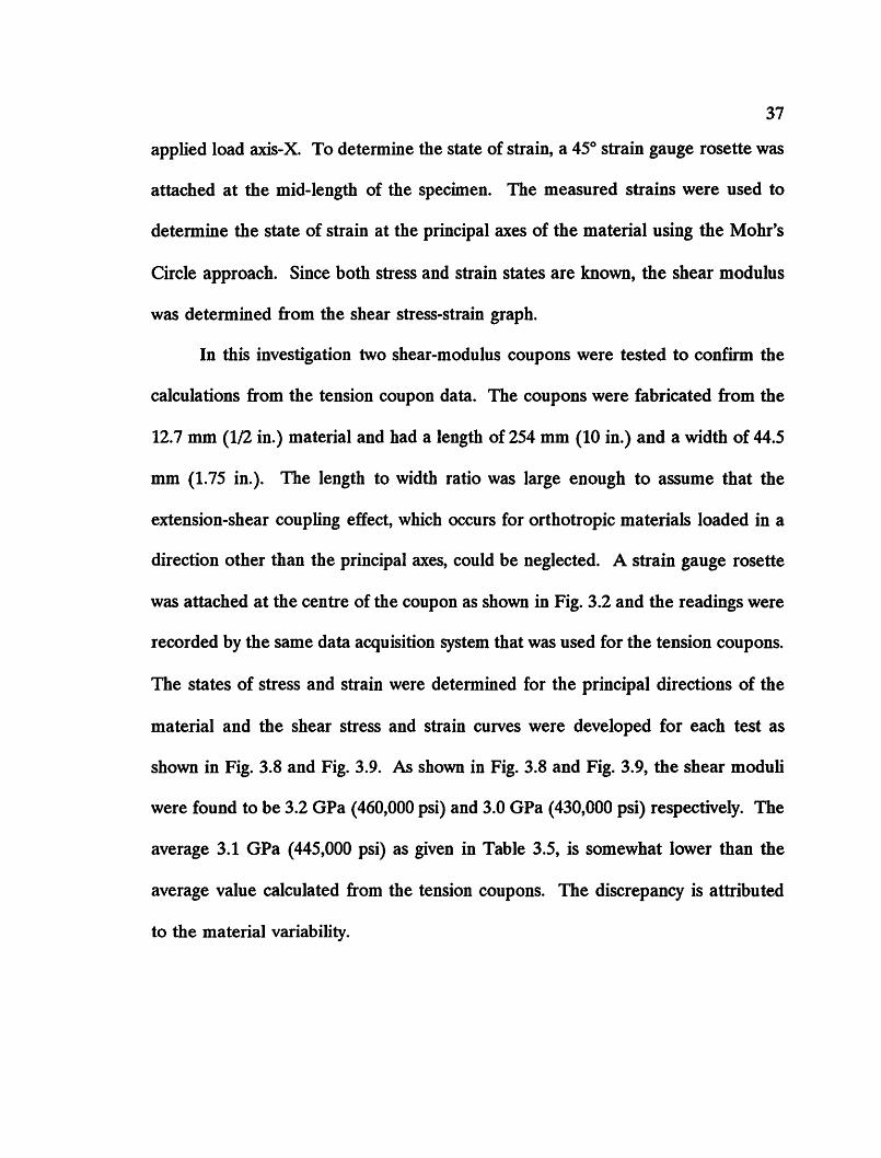
In this investigation two shear-modulus coupons were tested to confirm the

calculations from the tension coupon data. The coupons were fabricated from the

12.7 mm (1/2 in.) material and had a length of 254 mm (10 in.) and a width of 44.5

mm (1.75 in.). The length to width ratio was large enough to assume that the

extension-shear coupling effect, which occurs for orthotropic materials loaded in a

direction other than the principal axes, could be neglected. A strain gauge rosette

was attached at the centre of the coupon as shown in Fig. 3.2 and the readings were

recorded by the same data acquisition system that was used for the tension coupons.

The states of stress and strain were determined for the principal directions of the

material and the shear stress and strain curves were developed for each test as

shown in Fig. 3.8 and Fig. 3.9. As shown in Fig. 3.8 and Fig. 3.9, the shear moduli

were found to be 3.2 GPa (460,000 psi) and 3.0 GPa (430,000 psi) respectively. The

average 3.1 GPa (445,000 psi) as given in Table 3.5, is somewhat lower than the

average value calculated from the tension coupons. The discrepancy is attributed

to the material variability.

38

3.2.4 Compression Tests

A total of 75 compression tests were conducted according to ASTM Standard

D695. Figure 3.2(c) shows the typical dimensions of a compression coupon. The

length of the coupon was small enough to insure that the compressive strength was

not affected by buckling of the specimens. The average compressive strengths as

well as the standard deviations and coefficients of variation for each material

thickness at fibre orientations of 0° and 90° are given in Table 3.6. For the 12.7 mm

(1/2 in.) thick material, the compressive strength is given for various fibre angles

between 0° and 90°. It was found that the compressive strength of the 9.525 mm

(3/8 in.) thick specimens for the 0° fibre orientation, was slightly higher those of the

12.7 mm (1/2 in.) and 19.05 mm (3/4 in.) thick specimens. The results confirm that

the compressive strength is reduced as the fibre orientation increases from 0° to 90°.

3.2.5 Shear Tests

A total of 95 shear coupons were tested to determine shear strength. The

basic dimensions of the shear coupons are shown in Fig. 3.2( d). Sixty tests were

conducted according to ASlM Standard D3846 and thirty-five tests were conducted

according to a modified version of this standard. According to ASTM Standards

D3846, a compressive load is applied to the shear specimen to induce a shear failure

in the plane between the notches. Shear tests were conducted for all material

thicknesses and at 0° and 90° fiber orientations. The results are given in Table 3.7.

Similarly, it was found that the shear strength of the 9.525 mm (3/8 in.) material was

39

higher than those for the 12.7 mm (1/2 in.) and 19.05 mm (3/4 in.) materials. Table

3.7 shows that the shear strength for the 0° fibre orientation Fs13 and the shear

strength in the 90° fibre orientation Fs23 are fairly close in magnitude.

For bolted connections in composite materials, the material properties in the

plane of the members, the 1-2 plane, is important for the analysis. According to

ASTM Standard 03846 the notches are machined through the thickness of the

material to produce a shear plane that lies in the 1-2 plane of the material. A stress

analysis, as shown in Fig. 3.10( a), indicates that the measured shear strength is the

interlaminar shear strength Fs13 in the 1-3 plane, when the continuous fibres are at

0° to the applied load, and is the interlaminar shear strength Fs23 in the 2-3 plane,

when the fibres are at 90° to the applied load as shown in Fig. 3.10(b). Therefore,

the desired intralaminar shear strength Fs12 cannot be determined with the specimen

notches machined in this fashion. This is normally not a problem for a transversely

isotropic material, since Fs13=Fs12. However, for a material such as EXTREN Flat

Sheet which consists of different layers in the thickness direction and hence has

different properties in the 11211 and 11311 directions, the above equality is not valid. To

solve this problem, 35 shear coupons were tested with the notches machined through

the width-wise direction of the coupon as opposed to the thickness, as shown in Fig.

3.10(c). These IImodified" shear coupons were tested in the same manner as the

previous specimens. Machining the notches through the width-wise direction,

produced a shear plane parallel to the 1-3 material plane. A stress analysis shows

that by shearing through this plane, the strength that is measured is the desired

40

intralaminar shear strength F s12• Table 3.8 lists the results of the "modified" shear

tests. Comparing Table 3.7 and 3.8 it can be seen that the intralaminar shear

strength Fs12 is approximately 4 times higher than the interlaminar shear strength

Fs13• The "modified" shear coupons that were tested at angles other than 0° did not

fail through the shear plane and therefore their results are inconclusive as noted in

Table 3.8.

A summary of the in-plane material properties for EXTREN Flat Sheet is

given in Table 3.9 for the three thicknesses used in this investigation at fibre

orientations of 0° and 90°.

3.3 CONNECTION SPECIMENS

3.3.1 Parameters

The four basic geometric parameters studied in this investigation, which

influence the strength and failure mode of a connection, were the width of the

member, the edge distance, the thickness of the member, and the orientation of the

unidirectional fibres with respect to the applied load.

The effects of the width and the edge distance were effectively descnbed in

terms of dimensionless ratios with respect to the hole diameter. In this investigation

the hole diameter was kept constant at 20.6 mm (13/16 in.) for all of the tested

connections. The width and edge distance were varied to obtain different values for

the width to hole diameter ratio (wId) and the edge distance to hole diameter ratio

(e/d). The values of the width and edge distance were selected so that different

41

failure modes could be induced. The dimensions of the various parameters and

ratios are given in Table 3.10.

To determine the influence of the member's thickness on the behaviour of a

connection, three different thicknesses were used: 9.525 mm (3/8 in.), 12.7 mm (1/2

in.), and 19.05 mm (3/4 in.) as given in Table 3.10. These thicknesses were selected

as typical thicknesses applicable for structural members.

The fourth parameter, the angle of the unidirectional fibres with respect to

the applied load, can be considered to be partly a geometric parameter and partly

a material parameter. The structural shapes typically used in civil structures are

usually long and slender and therefore are ideally suited to be manufactured by the

pultrusion process. For this reason the principal load bearing fibres are usually

continuous and unidirectional and are oriented in the lengthwise direction of the

member. Random fibre mats are generally incorporated to provide transverse

strength. Unlike aeronautical structural members which tend to be skins and plates

and therefore can utilize multi-angle fibre lay-ups, pultruded structural shapes have

the continuous unidirectional fibres usually oriented only in the lengthwise direction

of the member. Since the bolt can bear at any angle with respect to the longitudinal

direction of the member and the unidirectional fibres, it was critical to study the

effects of this variable. In this investigation the 12.7 mm (1/2 in.) thick material was

used to fabricate connections that were tested with the principal unidirectional fibre

layers of the material at 0°, 45°, and 90° with respect to the applied load. The other

two thicknesses, 9.525 mm (3/8 in.) and 19.05 mm (3/4 in.), were tested with the

42

unidirectional fibres at 0° to the applied load.

It should be noted that the above parameters are not the only factors that

could influence the behaviour of bolted connections. Some of the more notable

ones may include the amount of clearance between the bolt and hole, the amount

of bolt torque or lateral pressure, the size of the washer, and bending effects caused

by single-shear instead of double-shear connections. In this investigation standard

washers with 19 mm (3/4 in.) high strength structural bolts were used. The hole

diameter of the connections was 20.6 mm (13/16 in.) providing a 1.6 mm (1/16 in.)

clearance for the bolt. This clearance was chosen as being typical of what is used

in the field and was kept constant throughout this investigation. The amount of

lateral pressure was also kept constant by tightening the bolt to a constant torque

of 32.5 N-m (24 ft-Ibs). This value is the recommended maximum installation

torque for FffiREBOLT Studs and Nuts as given in the EXTREN Design Manual

(70). Although the bolts used in this investigation were high strength steel bolts, the

same installation torque as that recommended for FffiREBOLT was used so that

a comparative study could be made with the different types of fasteners in a

subsequent investigation.

The experimental program consisted of 5 series of tests as shown in Table

3.11. The first series, Series A, included all the connections fabricated from the

9.525 mm (3/8 in.) material with the fibre angle at 0° or parallel to the applied load.

The next three series, B, C, and D consisted of the connections made from the 12.7

mm (1/2 in.) material with the fibre-load angle at 0°, 90°, and 45° respectively.

43

Series E consisted of the connections fabricated from the 19.05 mm (3/4 in.)

material with the fibre-load angle at 0°. The width and edge distance were varied

in an identical manner for each series producing 20 connection tests for each series

except for Series A for which two tests were repeated giving a total of 22 tests. The

test designations and various geometric dimensions are given for each connection

test in Table 3.11. A total of 102 connections were tested in this experimental

investigation.

3.3.2 Connection Fabrication

The connections tested in this investigation consisted of rectangular plates that

were cut from the large 1.2 x 2.4 m (4 x 8 ft.) sheets on a table saw equipped with

a carbide-tipped blade. The plates were cut to the desired width and to a length of

610 mm (24 inches) with an accuracy of ±1 mm (±1/32 inch). The length was

selected to be long enough to avoid the influence of end effects on the behaviour

of the connection and to produce a uniform applied stress at the mid-length.

To fabricate the connections that had the unidirectional fibres at 45° and 90°

to the applied load, the plates were laid out and cut at 45° and 90° to the

longitudinal or pultruded direction of the sheet.

At the end of the plate, a single bolt hole 20.6 mm (13/16 in.) in diameter was

marked out and drilled in the centre of the plate and at the desired edge distance.

At the far end of the plate, 19 mm (3/4 in.) diameter bolt holes were marked and

drilled to match the hole patterns in the upper steel gripping plate. Since the basic

44

configuration of the connections consisted of two composite plates, namely Plate A

and Plate B as described in § 3.4, both plates were clamped together and drilled

simultaneously to ensure alignment of the holes. Although more accurate methods

exist for fabricating these connections, such as reamed holes instead of drilled holes,

the methods utilized in this investigation more closely resemble what would be used

in the field.

3.4 TEST SET-UP

The connections were originally tested using a 270 kN (60,000 lb) RIEHLE

testing machine. Many of the specimens failed catastrophically and would incur

sudden load drops and displacement increases. It was found that the L VDT used

to measure the load for this particular machine, had a large lag effect and could not

accurately characterize the load drops which would normally occur in fractions of

a second. For this reason, all subsequent tests were preformed using a 1000 kN

(220,000 lb) MTS closed-loop selVo-controlled loading system. In this system the

loads were measured by a load cell which was more accurate in characterizing the

load-displacement behaviour of the connections tested. Tensile load was applied at

a constant stroke rate of 0.01 mm/sec (0.254 in/sec). The connections which were

tested on the RIEHLE machine are marked with an n*n in Table 3.11.

The test set-up shown in Fig. 3.11 was used to fit the test specimen to the

MTS loading system. The steel grips had a cup and cone shape which were

machined into the bearing plate and bearing nut respectively to allow for self

45

alignment as shown in Fig. 3.11. The steel grips also had several hole patterns to

allow for various sizes of the tested connections. For the tests performed on the

REIHLE machine, the grips were attached through the crossheads in a slightly

different manner.

An enlarged schematic of the connection set-up is shown in Fig. 3.12.

Photographs of the set-up are given in Fig. 3.13. The actual connection consisted

of two composites plates: Plate A and Plate B. The steel grips were placed between

the composite plates as shown in Fig. 3.12. The connection under investigation, the

"critical connection", was located at the lower end of the set-up and consisted of a

single-bolt in double-shear. The upper grip consisted of two steel clamping plates

that were used to "sandwich" the composite plates and the upper steel grip as shown

in Fig. 3.12. The applied tensile load was transferred from the upper grip assembly

to the composite plates through the clamping force and bearing action of two or

four bolts, depending on the width of the composite plates.

The two composite plate, double-shear configuration was selected to subject

the composite members to concentrically applied loading and to eliminate bending

effects. Most importantly, this type of "double specimen" arrangement simplified

strain and displacement measurements and allowed direct observation of the various

failure modes.

Throughout the connection set-up, 19 mm (3/4 in.) diameter ASlM A325 high

strength structural bolts and washers were used. The specified tensile strength of

the A325 bolts was 825 MPa (120,000 psi). For the larger connections 19 mm (3/4

46

in.) diameter SAE L9 high strength structural bolts were used. The specified tensile

strength of the SAE L9 bolts was 1240 MPa (180,000 psi). These bolts were used

on connections fabricated from the 19.05 mm (3/4 in.) thick material, where the

connection's load capacity exceeded 180 kN (40,000 lb). During the assembly of

each connection specimen, the bolts were carefully centred in the oversized holes.

In all cases, the bolt lengths were selected to ensure that both composite plates in

each connection intercepted the shank and not the threads of the bolt.

3.5 INSTRUMENTATION

To measure the relative displacement between the lower grip and the

composite plates, one LVDT (Linearly Variable Differential Transducer) was used

on each side of the connection as shown in Fig. 3.12. The L VDT's were mounted

on the lower grip and metal T -shapes were individually clamped to each composite

plate to align the L VDT's so as to measure the relative slip at the hole centre. The

load was measured by the load cell of the testing machine. The load and the two

displacement readings were recorded by a 40-channel Hewlett-Packard 3490A

Multimeter data acquisition unit and a Hewlett-Packard Vectra 286 Computer.

During each test, a Hewlett-Packard 7044A X-Y Recorder was used to produce an

X-Y plot of the load versus the average displacement. The arrangement of the

instrumentation as well as the loading system is shown in Fig. 3.14.

To measure the stress distribution at the net section, a total of 10 connections

were instrumented with strain gauges and are identified in Table 3.11. The strain

47

gauges were attached to Member A for each connection. A typical arrangement of

strain gauges is given in Fig. 3.15. The actual strain gauge arrangements for each

connection are documented in a separate technical report by the author, Rosner

(71). To measure strains close to the hole, a special washer was fabricated to

provide spaces for the gauges adjacent to the hole. The strain gauges used were

type CEA-06-250UN-350 manufactured by the Micro-Measurements Division of the

Measurements Group Inc. The gauges had a resistance of 350.0 ±0.3% ohms and

a gage factor of 2.070 ±0.5% at 24°C. The strain gauge readings were recorded by

the same system used for the load and displacement data. Most of the connections

selected to be instrumented with strain gauges had an edge distance equal to 101.6

mm (4 in.) and had widths varying from 101.6 mm (4 in.) to 254 mm (10 in.).

For connections that failed catastrophically, such as in net tension or cleavage

failure, the load reduction and displacement increases took place in fractions of a

second. To accurately characterize the load-displacement behaviour during such a

sudden event, a Tektronix 2214 Digital Storage Oscilloscope was used to record the

load and average displacement. Four connections, as listed in Table 3.11, were

continuously monitored with the oscilloscope at a sampling rate of 16,000 readings

per second. When a sudden failure occurred, the oscilloscope was manually

triggered to "freeze" the load and average displacement information which was then

downloaded to a personal computer for analysis.

Table 3.1 Tensile Strength

Thickness Fibre Number Tensile Strength nun Orientation of Average Standard Deviation Coeff. of (in.) (deg.) Tests (MPa) (psi) JMPa) (psi) Variation 9.525 0 10 198 28700 21.4 3100 0.108 (3/8) 45 5 121 17600 6.2 900 0.051

90 10 101 14700 6.7 976 0.066 12.7 0 10 166 24100 23.6 3430 0.142 (1/2) 30 5 114 16600 3.3 485 0.029

45 5 117 17000 4.0 581 0.034 60 5 110 15900 4.1 593 0.037 90 10 110 16000 8.3 1210 0.076

19.05 0 10 166 24100 27.2 3950 0.164 J3/4) 90 10 103 14900 5.5 793 0.053

Total: 80

Table 3.2 MDximum Tensile Strain

Thickness Fibre Number Maximum Tensile Strain Orientation of Average Standard Coeff. of

mm(in.) (deg.) Tests (%) Deviation Variation 9.525 0 10 1.6 0.06 0.04 (3/8) 45 5 1.7 0.06 0.04

90 10 1.2 0.17 0.14 12.7 0 10 1.6 0.16 0.10 (1/2) 30 5 1.4 0.05 0.04

45 5 1.6 0.08 0.05 60 5 16 0.22 0.14 90 10 1.4 0.11 0.08

19.05 0 10 1.6 0.16 0.10 (3/4) 90 10 1.4 0.09 0.07

Total: 80

Table 3.3 Tensile Modulus

Thickness Fibre Number Orientation of

mm (in.) (deg.) Tests 9.52S 0 10 (3/8) 4S S

90 10 12.7 0 10 (1/2) 30 S

4S S 60 S 90 10

19.0S 0 10 (3/4) 90 10

Total: 80

Average (GPa) (psi) lS.2 2.20E+06 9.8 1.42E+06 10.8 1.S6E+06 12.7 1.84E+06 11.6 1.68E+06 10.5 1.S2E+06 10.8 1.S7E+06 10.7 1.SSE+06 13.1 1.90E+06 11.1 1.61E+06

Elastic Moduli Standard Deviation (GPa) (psi)

3.1 4.51E+OS 0.4 6.10E+04 1.2 1.69E+OS 1.2 1.75E+OS 0.8 1.10E+OS 0.6 9.32E+04 1.1 1.S3E+OS 1.1 1.S4E+OS 2.4 3.41E+OS 1.3 1.91E+OS

Coeff. of Variation

0.20S 0.043 0.108 0.09S 0.066 0.061 0.098 0.099 0.179 0.199

Ut o

Table 3.4 Poisson's Ratios

Thickness Fibre Number Poisson's Ratios Orientation of Average Standard Coeff. of

mm (in.) (deg.) Tests (%) Deviation Variation 9.525 0 4 0.28 0.014 0.05 Major Poisson's Ratio (3/8) 90 3 0.21 0.051 0.24 Minor Poisson's Ratio

Table 3.5 Shear Modulus

Tension Shear Modulus (Calculated from Tension Coupon Results) Coupons Calculated Average Standard Deviation Coeff. of

iGPa) (psi) (GPa) (PsU Variation Thickness = 12.7 mm (1/2 in.) 4.2 605000 0.2 30100 0.05 Fibre Orient. =30, 45, 60 deg.

Thickness Fibre Number Shear Modulus (Measured from Shear Modulus Coupon~ Orientation of Average Standard Deviation Coeff. of

mm (in.) ideg.) Tests (GPa) (psi) (GPa) (psi) Variation 12.7 10 2 3.1 445000 0.15 21200 0.048 (1/2)

Table 3.6 Compression Strength

Thickness Fibre Number Compression Strength mm Orientation of Average Standard Deviation Coeff. of (in.) (deg.) Tests (MPa) (psi) (MPa) (psi) Variation 9.525 0 10 213 30900 13.6 1970 0.0638 {3/8) 90 10 145 21100 14.1 2040 0.0967 12.7 0 10 175 25400 12.2 1770 0.0697 (1/2) 30 5 159 23000 6.4 926 0.0403

45 5 159 23000 7.4 1070 0.0465 60 5 148 21500 7.4 1070 0.0498 90 10 145 21000 5.8 834 0.0397

19.05 0 10 157 22700 7.2 1050 0.0463 (3/4) 90 10 139 20200 8.6 1250 0.0619

Total: 75

Table 3.7 Interlaminar Shear Strength

Thickness Fibre Number Interlaminar Shear Strength mm Orientation of Average Standard Deviation Coeff. of (in.) (deg.) Tests (MPa) (psi) (MPa) (psi) Variation 9.525 0 10 32.3 4690 6.4 926 0.1970 (3/8) 90 10 37.2 5390 2.7 398 0.0738 12.7 0 10 27.8 4030 3.8 553 0.1370 (1/2) 90 10 24 3480 6.3 908 0.2610 19.05 0 10 27.6 4000 3.6 522 0.1310 (3/4) 90 10 27.9 4050 2.4 351 0.0867

Total: 60

Table 3.8 Intralaminar Shear Strength

Thickness Fibre Number Intralaminar Shear Strength mm Orientation of Average Standard Deviation Coeff. of (in.) (deg.) Tests (MPa) (psi) (MPa) (psi) Variation 9.525 0 5 116 16800 6.4 930 0.0554 (3/8) 12.7 0 5 104 15100 5.7 826 0.0547 (1/2) 30 5 115 16700 5.3 764 0.0457

45 5 120 17400 15.9 2300 0.1320 60 5 117 17000 2.5 358 0.0211 90 5 120 17400 7.4 1070 0.0615

19.05 0 5 114 16600 8.1 1180 0.0711 (3/4)

Total: 35

Table 3.9 Summary of Material Properties

Thickness Fibre Tensile Orientation Modulus

mm deg. GPa (in.) (Msi) 9.525 0 15.2 (3/8) (2.20)

90 10.8 (1.56)

12.7 0 12.7 (1/2) (1.84)

90 10.7 (1.55)

19.05 0 13.1 (3/4) (1.90)

90 11.1 (1.61)

Shear Modulus = 4.2 GPa Major Poisson's Ratio = 0.28

Tensile Strain

%

1.6

1.2

1.6

1.4

1.6

1.4

Tensile Compo Inter-Shear Intra-Shear Strength Strength Strength Strength

MPa MPa MPa MPa (psi) (psi) CJ!si1 (psi) 198 213 32.3 116.0

(28700) (30900) (4690) (16800) 101 145 37.2 ---

(14700) (21100) (5390) 166 175 27.8 104.0

(24100) (25400) (4030) (15100) 110 145 24.0 120.0

(16000) (21000) (3480) (17400) 166 157 27.6 114.0

(24100) (22700) (40001 (16600) 103 139 27.9 ---

(14900) (20200) (4050)

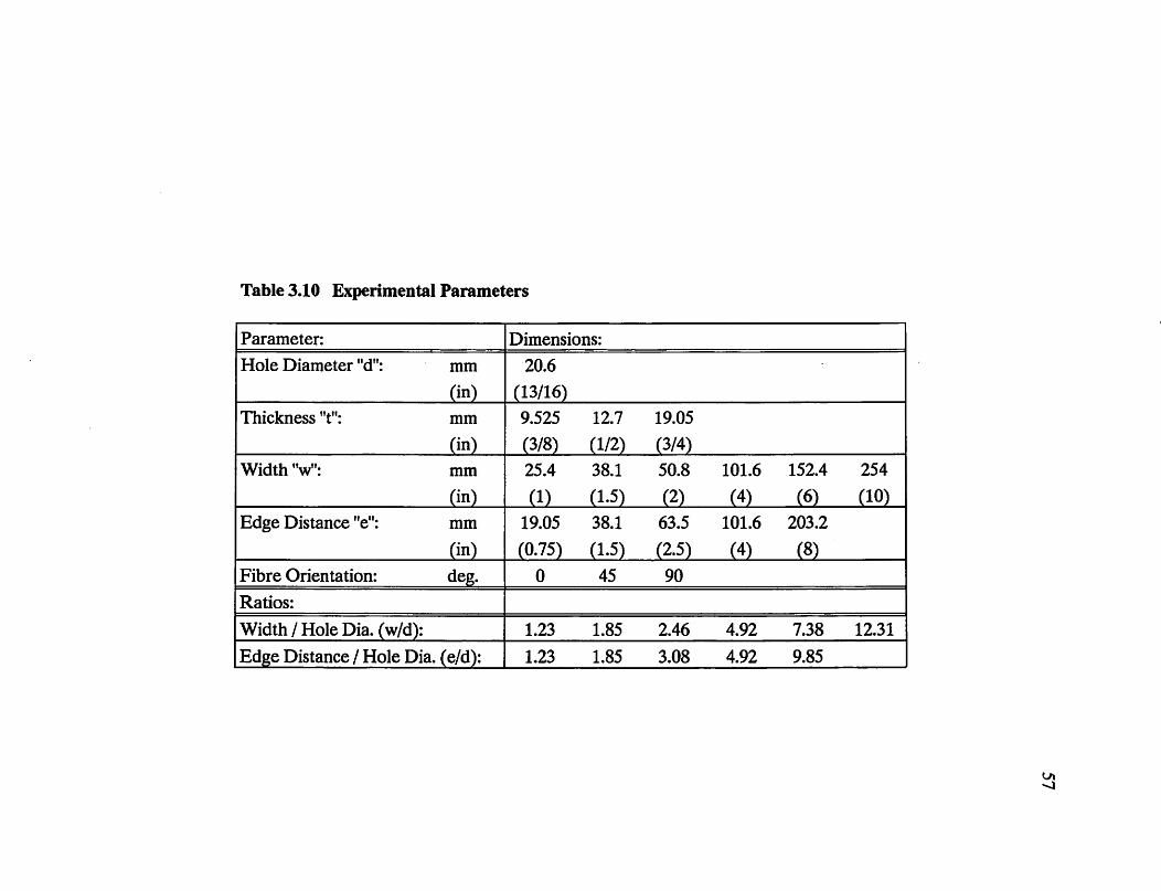
Table 3.10 Experimental Parameters

Parameter: Dimensions:

Hole Diameter "d": mm 20.6

(in) (13/16)

Thickness "t": mm 9.525 12.7 19.05

(in) (3/8) (1/2) (3/4)

Width "W": mm 25.4 38.1 50.8 101.6 152.4 254

(in) (1) (1.5) (2) (4) (6) (10)

Edge Distance "e": mm 19.05 38.1 63.5 101.6 203.2

(in) (0.75) (1.5) (2.5) (4) (8)

Fibre Orientation: deg. 0 45 90

Ratios:

Width / Hole Dia. (wId): 1.23 1.85 2.46 4.92 7.38 12.31

Edge Distance I Hole Dia. (e/d): 1.23 1.85 3.08 4.92 9.85

58

Table 3.11 Experimental Program

Test Parameter Dimensions mm (in.): RIEHLE Strain Oscilli-

Designation thickness "t" width "w" edge distance "e" Machine Gauges scope

& fibre angle m~ (in) mm (in)

Series A

A1 25.4 (1) 19.05 (0.75) • A2 203.2 (S) • A3 38.1 (1.5) • A4 38.1 (1.5) 635 (2.5) • AS 101.6 (4) • A6 38.1 (1.5) • A7 SO.S (2) 63.5 (2.5) Yes

AS 101.6 (4) • A9 38.1 (1.5) • A10 9.525 101.6 (4) 63.5 (2.5) • All (3/S) 101.6 (4) • A12 @Odeg. 203.2 (S) • A13 38.1 (1.5) • A14 152.4 (6) 63.5 (2.5) • A1S 101.6 (4) • A16 19.05 (0.75) • A17 38.1 (1.5) • A1S 254 (10) 63.5 (2.5) • A19 101.6 (4) • Yes

A20 203.2 (S)

A21 101.6 (4) 101.6 (4) Yes Yes I

A22 152.4 (6) 101.6 (4) • Yes

Series B

B1 25.4 (1) 19.05 (0.75) • B2 203.2 (S) • B3 38.1 (1.5) • B4 3S.1 (1.5) 63.5 (2.5) • BS 101.6 (4) • B6 38.1 (1.5) • I

B7 50.S (2) 63.5 (2.5) • BS 101.6 (4) • B9 12.7 38.1 (1.5) • BI0 (1/2) 101.6 (4) 63.5 (2.5) Yes

Bll @Odeg. 101.6 (4) • B12 203.2 (S)

B13 38.1 (1.5) • B14 152.4 (6) 63.5 (2.5) • B15 101.6 (4) • B16 19.05 (0.75) B17 38.1 (1.5) B1S 254 (10) 63.5 (2.5) Yes

I

B19 101.6 (4) Yes I B20 203.2 (S)

59

Table 3.11 Experimental Program (cont'd)

Test Parameter Dimensions mm (in.): RIEHLE Strain Oscilli-

Designation thickness "t" width ''w" edge distance "e" Machine Gauges scope

& fibre angle mm (in) mm (in)

Series C

Cl 25.4 (1) 19.05 (0.75)

C2 203.2 (8)

C3 38.1 (1.5)

C4 38.1 (1.5) 63.5 (2.5) • CS 101.6 (4)

C6 38.1 (1.5)

C7 50.8 (2) 63.5 (2.5) • C8 101.6 (4)

C9 12.7 38.1 (1.5)

CI0 (1/2) 101.6 (4) 63.5 (2.5) • C11 @90deg. 101.6 (4)

C12 203.2 (8)

C13 38.1 (1.5)

C14 152.4 (6) 63.5 (2.5) • C15 101.6 (4) Yes

C16 19.05 (0.75)

C17 38.1 (1.5)

C18 254 (10) 63.5 (2.5)

C19 101.6 (4) Yes

C20 203.2 (8)

Series 0

01 25.4 (1) 19.05 (0.75)

02 203.2 (8)

03 38.1 (1.5)

04 38.1 (1.5) 63.5 (2.5) • 05 101.6 (4)

06 38.1 (1.5)

07 50.8 (2) 63.5 (2.5) • 08 101.6 (4)

09 12.7 38.1 (l.5) 010 (1/2) 101.6 (4) 63.5 (2.5) • 011 @45deg. 101.6 (4)

012 203.2 (8)

013 38.1 (1.5)

014 152.4 (6) 63.5 (2.5) • 015 101.6 (4) 016 19.05 (0.75) 017 38.1 (1.5) 018 254 (10) 63.5 (2.5) 019 101.6 (4) 020 203.2 (8)

60

Table 3.11 Experimental Program (cont'd)

Test Parameter Dimensions mm (in.): RIEHLE Strain OsciUi-

Designation thickness "t" width "w" edge distance "e" Machine Gauges scope & fibre angle mm (in) mm (in)

Series E

E1 25.4 (1) 19.05 (0.75)

E2 203.2 (8)

E3 38.1 (1.5) E4 38.1 (1.5) 63.5 (25) ES 101.6 (4) E6 38.1 (1.5) E7 50.8 (2) 63.5 (2.5) E8 101.6 (4) E9 19.05 38.1 (1.5) E10 (3/4) 101.6 (4) 63.5 (25) Ell @Odeg. 101.6 (4) Yes E12 203.2 (8) E13 38.1 (1.5) E14 1524 (6) 63.5 (25) E15 101.6 (4) Yes E16 19.05 (0.75) E17 38.1 (1.5) E18 254 (10) 63.5 (25) E19 101.6 (4) Yes E20 203.2 (8) Yes

Total = 102 Connection Tests

X Applied Load Axis

1

Principal Material

Axis

2

Figure 3.1 Load Axes and Principal Material Axes

61

y

62

Gauge Length=50 mm t=9.525, 12.7, 19.05 mm

width = 12.7 mm Strain Gauges

radius=76 mm

(a) Tension Coupon Dimensions (ASTM 0638)

Fibre Angle = 10 deg

x Rosette

1

y 2

Length=254 mm

(b) Shear Modulus Coupon Dimensions

Figure 3.2 Material Coupon Dimensions

width= 12.7 mm

Thickness: Length: 9.525 mm ............ 38.1 mm 12.7mm ............. 50mm 19.05 Mm ............ 50 mm

(c) Compression Coupon Dimensions (ASTM D695)

Coupon Dimensions: width = 12.7 mm Ll=79.5mm L2=L3=36.3 mm lA=6.4mm

lA

Ll

thickness=9.525, 12.7, 19.05 mm n1=n2=t/2 Notch width = 1.02 to 1.65 mm

(d) Shear Coupon Dimensions (ASTM D3846)

Figure 3.2 Material Coupon Dimensions (cont'd)

63

64 200

180

160

140 "........ 120 (U

$1 100 "-'

CIl

~ 80 .. CIl

60

40

20

0.2 0.4 0.6 0.8 1 1.2 1.4 1.6 Strain (%)

Figure 3.3 Stress-Strain Curves for Material Thickness t=9.525 nun

200

180

160

140 "........ 120 (U

$1 100 "-'

CIl

~ 80 .. CIl

60

40

20

0.2 0.4 0.6 0.8 1 1.2 1.4 1.6 Strain (%)

Figure 3.4 Stress-Strain Curves for Material Thickness t=12.7 mm

200

180

160

140

".-..,

120 "" ~

100 ~

VJ e 80 .....

CIl

60

40

20

00 0.2 0.4 0.6 0.8 1 1.2 1.4 1.6 Strain (%)

Figure 3.5 Stress-Strain Curves for Material Thickness t=19.05 mm

18~----------------------------------------~

16 Tension Specimen T38-C5-AO-S1

"'-"'8 14 .g ~ 12 ~

0 10 0 v

VJ c: .- 8 ~ ~ .....

CIl

~ 6 ~

~ < 4

2

0 0

Major Poisson Ratio =0.156/0.569 =0.27

Avg. Long. Strains Slope=0.569 (1/kN)

Avg. Trans. Strains Slope=0.156 (1/kN)

4 8 12 16 20 24 Applied Load (leN)

Figure 3.6 Determination of Major Poisson's Ratio

28

65

6~-----------------------------------------'

Tension Specimen T38-C6-A90-S2 • 5

e Minor Poisson Ratio =0.150/0.766=0.20 ~ § 4 ~

8 .....;" ~ 3 Avg. Long. Strains ·f Slope=0.766 (1/kN) ~

CIl ~ 2 Avg. Trans. Strains e Slope=0.150 (1/kN) ~ «

1

O~~~~~~~--~~--~

~

] '-' til

~ ~

CIl .... = QJ ..c: CIl

o 1 2 3 4 5 6 7 Applied Load (leN)

Figure 3.7 Determination of Minor Poisson's Ratio

14

12

10

8

6

4

2

~ ~ l/

v (~ = 3.2 GPa

1"'-

/ V V

/ V V Loa ~, /

/ V V /

V / Un oad /v

~ V Shear Modu usSpe cimen: CI-Al ()-S2

o o 0.5 1 1.5 2 2.5 3 3.5

Shear Strain (.001 mm/nun) 4 4.5 5

Figure 3.8 Shear Stress-Strain Graph for Shear Modulus Specimen #1

66

67

25~--~----~----~--~----~----~--~----~

20

-. ~

~ 15 --.,;'

tn tn

~ ....,a Q) .... 10 ~ OJ ..c::

Q)

5+-----~~~~~~----4-----+-----~--~----~

Shear odulus Specim : C2-A O-S2

1 2 3 456 7 8 Shear Strain (.001 mm/mm)

Figure 3.9 Shear Stress-Strain Graph for Shear Modulus Specimen #2

3

tLl E:::;71

68

3 Shear Coupon ASTM 03846

1 1

(a)

3

(b)

1

(c)

Fibre Orientation= 0 deg. Measured Shear Strength Fs(13).

Shear Coupon ASTM 03846 Fibre Orientation = 90 deg. Measured Shear Strength Fs(23).

Modified Shear Coupon Fibre Orientation = 0 deg. Measured Shear Strength Fs(12).

Figure 3.10 Stress Analysis of Shear Coupons

I" Dia. Allen Bolts

1" Dia. Threaded Rod

Piston Head and Load Cell

7" x T' x 2" Plate (Shown twice for assembly detail.)

Hex Nuts r-"t~=t-----I--+- Cup and Cone

---+-4----~mr~--

Upper Grip Plate

Lower Grip Plate

BasePlate

• •••• •

• •

Upper Bearing Plate

Lower Bearing Plate

LrrrtFwr;;:::f----r--r- Cup and Cone

Figure 3.11 Load Frame and Gripping System

69

70

Steel Grips

ee

Composite Plates

Critical

Figure 3.12 Test Set-up

71

Front Side

Figure 3.13 Connection Configuration

72

Figure 3.14 Instrumentation and Loading System

73

2 1 Dimensions = mm

9.5 76.2

152.4 304.8

6 4 3 5 7

101.6

25.4 12.7 6.4

Figure 3.15 Typical Strain Gauge Arrangement

· CHAPTER 4 TEST RESULTS AND DISCUSSION

4.1 TEST RESULTS

This chapter presents the test results of a total of 102 single-bolted

connections tested in this investigation. The measured ultimate load and mode of

failure for all of the connections tested are summarized in Table 4.1. The ultimate

load is the total capacity of the connection based on the two composite plate

members it is comprised of. The failure mode is also given for each plate member

in the connection.

In Series A., two connections, All and A15 were repeated and marked A2l

and A22 respectively to determine the variability of the results. In general the

failure modes corresponded for both pairs of tests. As given in Table 4.1, the

ultimate load of connections All and A21 varied approximately 10% and the

ultimate load of connections A15 and A22 varied by only 5%. The variability of the

test results is acceptable, since it is within the range of material variability. The

ultimate strengths of connections, when normalized with respect to the thickness of

the material, generally corresponded with one another and confirmed that the

variability of the connection test results was within the variability range of the

material properties.

74

75

4.2 FAILURE MODES

Three of the four basic failure modes were obsetved in this investigation as

shown in Fig. 4.1. The three modes were net-tension failure as shown in Fig. 4.1(a),

cleavage failure as shown in Fig. 4.1(b), and bearing failure as shown in Fig. 4.1(c).

Net tension failure was characterized by typical fracture through the net section.

Cleavage failure was characterized by a crack parallel to the applied load

propagating from the end of the plate towards the bolt hole leading to the initiation

of other cracks near the net section due to the formation of in-plane bending

stresses. Bearing failure was characterized by crushing of the material in the vicinity

of the bolt-to-hole interface.

Combinations of the three basic failure modes were also obsetved. Combined

bearing-net tension failure, bearing-cleavage failure, and cleavage-net tension failure

are shown in Fig. 4.2(a), (b), and (c) respectively.

Due to the high percentage of random fibres in the material used in this

investigation, the shearout mode of failure was not obsetved. This failure mode

required very small edge distances that were impractical.

4.3 LOAD-DISPLACEMENT CHARACTERISTICS

A comparison of typical load-displacement relationships for the three basic

modes of failure are shown in Fig. 4.3. The displacement is the average reading of

the two L VDTs mounted on either side of the connection. The load is the total

resistance of the two plate members comprising each connection.

76

The behaviour shown in Fig. 4.3, reflects a small initial friction resistance

capacity of the connection due to the applied bolt torque of 32.5 N-m (24 ft-Ib).

Slipping of the connections occurred at the initial loading stage. Once the bolt

slipped into bearing, all of the connections behaved linearly. Fig. 4.3 illustrates a

step-function behaviour characterizing the sudden drop in load carrying capacity for

the net tension and cleavage failure modes. The load drops typically occurred in

two distinct "events" as the two composite plates comprising each connection would

not fracture at the same time. For connections that failed in bearing, the load

reduction occurred gradually as the bolt pulled through the composite plates

simultaneously and the overall behaviour was much more ductile than the other

modes of failure.

Load-displacement curves for the combined failure modes are shown in Fig.

4.4 to Fig. 4.6. The behaviour of a connection that failed in combined bearing

cleavage is compared to the behaviour of a similar connection that failed in bearing

as shown in Fig. 4.4. The behaviours of the two connections are essentially the same

with the only difference occurring in the post-failure stages where cleavage failure

occurs for the combined mode reducing the overall ductility.

The load-displacement behaviour for a connection that failed in combined

bearing-net tension failure is compared to a connection that failed in net tension as

shown in Fig. 4.5. The behaviour is almost identical, however, the larger width of

the members used for specimen Bt2 allowed the connection to gain additional

capacity through bearing before the net tension failure occurred.

77

The behaviour of a connection that failed in combined cleavage-net tension

is shown in Fig. 4.6. As shown in Table 4.1, this combined mode was only observed

for the connections with members having a fibre orientation of 45° with respect to

the applied load. The behaviour is compared to both a pure net tension failure case

and a cleavage failure case for similar connections with the same fibre orientation.

The behaviour of the combined case is located between that of the two basic failure

modes. The increase in the load capacity in comparison to the cleavage case is due

to an increase in the edge distance. The higher load for the net tension case is

again due to an increase in the edge distance.

In most cases, the slippage, which occurred as a result of the bolt being

centred in an oversized bolt hole, had progressed in one step. The load increased

until the friction forces between the composite plates and the washers and the lower

steel grip were overcome, causing the load to plateau and the displacement to

increase as the slippage took place. The slippage was approximately equal to half

the clearance between the bolt and the oversized hole.

In some connection tests the slippage had occurred in two steps as shown in

Fig. 4.7. The first step occurred when the composite plate members, along with the

bolt, slipped with respect to the lower grip plate. Therefore, the slip distance of the

first step was normally equivalent to the small clearance that existed between the

bolt and the hole of the lower steel grip. The second slippage step occurred as the

composite plates slipped with respect to both the lower grip and the bolt, leading

to a larger slip distance approximately equal to half the clearance between the bolt

78

and the holes in the composite plates.

Catastrophic failure modes, such as net tension and cleavage, usually took

place in fractions of a second. This usually meant that the load-displacement

behaviour between the time that the failure was initiated and the time that it

stopped could not be recorded unless a very fast data acquisition system was used.

To accurately characterize such a sudden event, a storage oscilloscope was used to

monitor the signals from the load and displacement transducers. Figure 4.8

represents the data recorded on the oscilloscope screen. Both the load resistance

and the average displacement readings were recorded in the same figure with

respect to time. In this case the selected time interval "frozen time" was 1 second.

The vertical axis in Fig. 4.8 represents the resolution of the oscilloscope as the

number of oscilloscope divisions. For the load signal, one level is equal to 1 kN

(224.8 lb) and for the displacement signal, one level equals 0.508 mm (.002 in.). The

failure event is enlarged using a larger time scale as shown in Fig 4.9 where the load

and displacement data are given for a time interval of 0.1 seconds. The oscillations

in the displacement signal are the result of electronic noise from the displacement

transducers and should be ignored. The damped oscillations in the load signal right

after the drop in load are a result of the physical response of the load cell to the

fracture impulse and should also be ignored. The failure event occurs as the load

instantly drops a certain amount and the displacement increases over a certain time

interval. These signals can be modelled using linear segments as shown in Fig. 4.10.

Using the modelled curves and the conversion factors, the load and displacement

79

readings during the failure event can be plotted on a load-displacement graph. This

curve·can then be superimposed onto the load-displacement graph recorded by the

slower data acquisition system as shown in Fig. 4.11. The L-shaped load-

displacement cUlVe recorded by the oscilloscope is the correct behaviour of a

connection during a catastrophic failure event and is typical of all the connections

tested in this investigation which failed in a sudden manner.

4.4 ULTIMATE STRENGTHS

To analyze the results of the connection tests, the following average ultimate

strengths are defined as:

Pull Ultimate Bearing Strength ... ---dboll (2t)

Pull Ultimate' Net Tension Strength - ___ _ (w-d) (2t)

(4.1)

(4.2)

In Eq.( 4.1) and (4.2), P ult is the ultimate failure load, taken as the maximum load

attained during a connection test. The variables w, d, dbolt and t are the member

width, the hole diameter, the bolt diameter and the material thickness of a

connection respectively. Since each connection is comprised of two composite

plates, the thickness is multiplied by two in Eq.(4.1) and (4.2).

80

4.5 EFFECT OF WIDTH

Variation of the width of the members in a connection predominantly

influences the capacity of a connection as well as the corresponding mode of failure.

For connections comprised of members with a 00 fibre orientation, the ultimate

bearing strength with respect to the width-to-hole-diameter ratio (wid) is given in

Fig. 4.12 to Fig. 4.14 for Series A, B, and E respectively. For comparative purposes

the same results are given in Fig. 4.15 for all of the above series. The various failure

modes are represented as "NTI for net tension, "C" for cleavage, and "B" for bearing

with the combined modes represented by hyphenated letters. The lines in Fig. 4.12

to Fig. 4.15 are given for connections with the same edge distance. For connections

with relatively small edge distances, the mode of failure changes from net tension

failure to cleavage failure as the (wid) ratio increases. For connections with

relatively large edge distances, the mode of failure changes from net tension failure

to bearing failure. Associated with the change in failure mode is an increase in

bearing strength as the (wid) ratio increases. The strength increases tend to level

off past (w/d)=5 which is within the range of typical values for composite materials

given in Chapter 2. The transition between failure modes is not sharply defined as

shown in Fig. 4.12 to Fig. 4.15, since the connections within the transition zones are

influenced by combined modes of failure.

The ultimate net tension strengths for connections with various edge distances

of Series A, B, and E are plotted with respect to the (wid) ratio in Fig. 4.16. The

lines in Fig. 4.16 represent connections with the same edge distance. The net

81

tension strengths of connections with large (wId) ratios are relatively small compared

to the net tension strengths of connections with small (wId) ratios. This behaviour

is mainly due to the high magnitude of stress concentrations for members with large

widths. These stress concentrations can be in the order of 4 to 6 as will be

discussed. For the narrow connections, with relatively small (wId) ratios, the net

stress concentrations are more moderate, in the order of 2 to 3, thereby allowing

higher net tension strengths to be achieved.

4.6 EFFECT OF EDGE DISTANCE

To illustrate the effects of variation in edge distance, the ultimate bearing

strengths of the connections are plotted with respect to the edge-distance-to-hole

diameter ratio (e/d) in Fig. 4.17 to Fig. 4.19 for Series A, B, and E respectively. The

results for all three series are combined and shown in Fig. 4.20. The lines in Fig.

4.17 to Fig. 4.20 are given for connections with the same width. For narrow

connections, the variation of edge distance has little effect on the failure mode or

ultimate strength as shown in Fig. 4.17 to Fig. 4.20, where the predominant failure

mode is net tension regardless of the size of the edge distance. However, for wider

connections, the failure mode changes from cleavage failure to bearing failure with

increasing (e/d) ratios. The results indicate that the ultimate bearing strength

increases with an increase in the (e/d) ratio up to a value of (e/d) =5. This value is

within the range of typical values for composite materials. Again the transition

between failure modes is not sharply defined.

82

The ultimate net tension strengths for the connections of Series A, B, and E

are plotted with respect to the (e/d) ratio in Fig. 4.21. The lines in Fig. 4.21 are

given for connections with the same width. With an increasing (e/d) ratio, the

ultimate net tension strengths tend to increase up till a value of (e/d)=5. This

suggests that increasing edge-distances tend to reduce the stress concentrations

associated with net stresses and therefore increase the net tension strength capacity.

4.7 EFFECT OF THICKNESS

. For the three material thicknesses used in this investigation, the results

indicate that the member thickness had little effect on the overall behaviour of the

connections. This is demonstrated in Figures 4.15, 4.16, 4.20, and 4.21, which show

the results of 00 connections for all three material thicknesses. The ultimate

strengths of the connections for different thicknesses tend to match within the range

of material variability. The failure modes of connections with the same geometry

but different thicknesses also correspond.

The lateral constraint applied by the washers reduces the influence of the

member thickness on the connection behaviour. It seems that high strength

structural bolts tightened to a torque of 32.5 N-m (24 ft-lbs) as used in this

investigation, are adequate to remove most of the influence of the material

thickness.

83

4.8 EFFECT OF FIBRE ORIENTATION

The influence of fibre orientation on the modes of failure is shown in Fig. 4.22

for connections of the same dimensions. Due to the presence of the unidirectional

fibres at 450 and 900 to the applied load, the typical cleavage failure that had

occurred in connections with a 00 fibre orientation as shown in Fig. 4.22( a), was

suppressed for the corresponding connections that had a fibre orientations of 450

and 900 to the applied load as shown in Fig. 4.22(b) and (c).

The load-displacement behaviours of the connections in Fig. 4.22 are given in

Fig. 4.23. Although the ultimate loads of the 450 and 900 connections were lower

than their 00 counterparts, the general shape of the load-displacement curves

remained unchanged.

The ultimate bearing strengths of connections with a fibre orientation of 450

and 900 are plotted with respect to the (wId) ratio in Fig. 4.24 and Fig. 4.25

respectively. The lines represent connections with the same edge distance. As

shown in the figures and in Table 4.1, the predominate mode of failure is net

tension regardless of the connection geometry. Only in the extreme ranges of the

geometrical dimensions do the failure modes change to cleavage and bearing. For

large widths and very small edge distances, cleavage failure occurred and for large

widths and large edge distances, bearing failure occurred as shown in Fig. 4.24 and

4.25. The 450 case seems to be more susceptible to combined failure modes

suggesting that at this fibre orientation there is a larger interaction between the

stresses corresponding to each basic failure mode.

84

The ultimate bearing strengths with respect to the (wid) ratio of the 450 and

900 fibre orientation connections are compared to the results for the 00 connections

of the same thickness in Fig. 4.26. The increases in bearing strength with increasing

(wid) ratio, begin to level off past (w/d)=5. However, the results suggest that to

achieve bearing failure the (wid) value must be larger. Figure 4.26 illustrates the

reduction in bearing strength with the change in fibre orientation from 00 to 900•

The results in Fig. 4.26 are given for those edge distances which best reflect the

effects of the fibre orientation. From the ultimate loads given in Table 4.1 it can

be shown that a change in fibre orientation from 00 to 900, reduces the bearing

strength approximately 18% for the 450 case and 24% for the 900 case. For the

connections with small (wid) ratios the predominant failure mode was net tension

for all fibre orientations. At higher (wid) ratios, the predominant failure mode was

either bearing or cleavage failure for the 00 case but remained net tension failure for

the 450 and 900 cases due to their high susceptibility to net tension fracture, as

shown in Fig. 4.26.

The ultimate bearing strengths for the 450 and 900 connections are plotted

with respect to the (e/d) ratio in Fig. 4.27 and 4.28 respectively. The lines in Fig.

4.27 and 4.28 are given for connections with constant width. As with the 00

connections, the bearing strengths of the 450 and 900 connections tended to increase

with increasing (e/d) ratios up till a value of (e/d) =5. Again the results suggest that

to achieve bearing failure in the 450 and 900 cases the (e/d) ratio must be larger.

The bearing strengths with respect to the (e/d) ratios for the three fibre

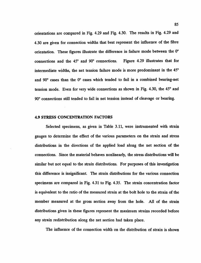
85

orientations are compared in Fig. 4.29 and Fig. 4.30. The results in Fig. 4.29 and

4.30 are given for connection widths that best represent the influence of the fibre

orientation. These figures illustrate the difference in failure mode between the 0°

connections and the 45° and 90° connections. Figure 4.29 illustrates that for

intermediate widths, the net tension failure mode is more predominant in the 45°

and 90° cases than the 0° cases which tended to fail in a combined bearing-net ,

tension mode. Even for very wide connections as shown in Fig. 4.30, the 45° and

90° connections still tended to fail in net tension instead of cleavage or bearing.

4.9 STRESS CONCENTRATION FACTORS

Selected specimens, as given in Table 3.11, were instrumented with strain

gauges to determine the effect of the various parameters on the strain and stress

distributions in the directions of the applied load along the net section of the

connections. Since the material behaves nonlinearly, the stress distributions will be

similar but not equal to the strain distributions. For purposes of this investigation

this difference is insignificant. The strain distributions for the various connection

specimens are compared in Fig. 4.31 to Fig. 4.35. The strain concentration factor

is equivalent to the ratio of the measured strain at the bolt hole to the strain of the

member measured at the gross section away from the hole. All of the strain

distributions given in these figures represent the maximum strains recorded before

any strain redistribution along the net section had taken place.

The influence of the connection width on the distribution of strain is shown

86

in Fig. 4.31 and Fig. 4.32 for member thicknesses of 9.252 mm (3/8 in.) and 19.05

mm (3/4 in.) respectively. The figures illustrate that in general, increases in member

width increase the strain concentration factors. This is obvious in the case of the

254 mm (10 in.) wide connections where the strain concentration factor adjacent to

the hole approaches a value of 6, in comparison to the 101.6 mm (4 in.) wide

connections where the strain concentration factor approaches the value of 2. These

results are in agreement with the theoretical deductions of Hart-Smith (39). Since

the applied stress at the gross section away from the hole must be reacted by the

bolt, most of the load is resisted by the material in the vicinity of the hole. This is

shown in the 254 mm (10 in.) wide connections, where the strain distributions are

well below unity near the sides of the plate and are essentially zero at the free edge.

The strain distributions confirm that the structural efficiency of a connection is

highly dependent on the width of the plate.

The influence of the edge distance on the strain distribution is shown in Fig.

4.33. The connections shown are identical except for the edge distances. The

connection with the 203.2 mm (8 in.) edge distance has lower strain concentrations

than the one with the 101.6 mm (4 in.) edge distance. The larger edge distance

seems to allow the material at the net section to be used more efficiently as the

stresses are not forced to "flow" as close to the bolt hole as in the case of small edge

distance. Overall it seems that the edge distance does not have as great an influence

on the strain distributions as the width does.

The effect of the material thickness on the strain distribution seems to be

87

negligible as shown in Fig. 3.34. The connections shown are identical except for the

material thickness. The maximum strain concentration factor is in the range of 5

to 6 for the three thicknesses.

Fibre orientation has a marked effect on the strains as shown in Fig. 4.35

which gives the distributions for 00 and 900 connections. The strain distribution

away from the hole does not seem to be influenced as much as the strain

concentrations near the hole. For connections with the same geometry, the

maximum strain concentration factor adjacent to the hole is approximately 6 for the

00 fibre orientation connection and approximately 7.5 for the 900 fibre orientation

connection. The higher strain concentrations coupled with the lower tensile strength

in the direction of the applied load both contribute to the lower ultimate loads

experienced by the "angled" connections.

Table 4.1 Test Results

Test Parameter Dimensions mm (in.): Ultimate Failure

Designation thickness "t" width "w" edge distance "e" Load Mode

& fibre angle mm (in) mm (in) kN (lbs) Plate A I Plate 8

Series A

Al 25.4 (1) 19.05 (0.75) 12.2 2750 NT NT

A2 203.2 (B) 14.5 3250 NT NT

A3 38.1 (1.5) 44.0 9900 NT NT

A4 38.1 (1.5) 63.5 (25) 43.B 9850 NT NT

AS 101.6 (4) 39.4 8850 NT NT

A6 38.1 (1.5) 55.3 12425 NT NTI

A7 50.B (2) 63.5 (2.5) 57.B 12990 NT NT

AB 101.6 (4) 61.3 13775 NT NT

A9 38.1 (1.5) 69.2 15550 C C

A10 9.525 101.6 (4) 63.5 (2.5) 95.3 21425 B-NT B-NT !

All (3/B) 101.6 (4) 103.0 23150 B-NT 8-NT

A12 @Odeg. 203.2 (B) 100.5 22600 B-NT 8-NT

A13 38.1 (1.5) 67.6 15200 C C

A14 152.4 (6) 63.5 (25) 109.4 24600 C C

A15 101.6 (4) 129.0 29000 B-NT 8

A16 19.05 (0.75) 28.9 6500 C C

A17 38.1 (1.5) 66.7 15000 C C

AlB 254 (10) 63.5 (2.5) 113.0 25400 C C

A19 101.6 (4) 116.8 26250 8 8

A20 203.2 (8) 113.9 25600 8 B

A21 101.6 (4) 101.6 (4) 921 20700 B B-NT

A22 152.4 (6) 101.6 (4) 122.8 27600 8 8

Series 8

81 25.4 (1) 19.05 (0.75) 13.3 3000 NT NT

82 203.2 (B) 14.9 3350 NT NT

83 38.1 (1.5) 52.3 11750 NT NT

84 38.1 (1.5) 63.5 (2.5) 60.5 13600 NT NT

B5 101.6 (4) 54.9 12350 NT NT

B6 38.1 (1.5) 72.9 16400 NT NT

87 50.8 (2) 63.5 (2.5) 75.4 16950 NT NT

8B 101.6 (4) B3.4 18750 NT NT

89 12.7 38.1 (1.5) 97.5 21925 C C 810 (1/2) 101.6 (4) 63.5 (2.5) 115.1 25870 8-NT B-NT

811 @Odeg. 101.6 (4) 145.0 32600 B-NT 8-NT B12 203.2 (B) 137.9 31010 B-NT 8-NT B13 38.1 (1.5) 95.2 21400 C C 814 152.4 (6) 63.5 (2.5) 152.6 34300 C C B15 101.6 (4) 167.2 37600 B B 816 19.05 (0.75) 36.6 B225 C C B17 38.1 (1.5) 101.1 22740 C C BIB 254 (10) 63.5 (2.5) 133.9 30100 C C 819 101.6 (4) 184.1 41400 8-NT 8 820 203.2 (8) 186.0 41810 8 B Failure Modes: NT=Net Tension C=Cleavage 8=Bearlng B-NT=Combined Bearing-Net Tension

8-C=Combined Bearing-Cleavage C-NT=Combined Cleavage-Net Tension

88

Table 4.1 Test Results (cont'd)

Test Parameter Oimensions mm (in.): Ultimate Failure

Oesignation thickness "t" width 'V/' edge distance "e" Load Mode

& fibre angle mm (in) mm (in) kN (lbs) Plate A .1 Plate B

Series C

C1 25.4 (1) 19.05 (0.75) 11.8 2650 NT NT

C2 203.2 (8) 11.7 2630 NT NT

C3 38.1 (1.5) 34.9 7840 NT NT

C4 38.1 (1.5) 63.5 (2.5) 28.7 6450 NT NT

C5 101.6 (4) 32.1 7210 NT NT

C6 38.1 (1.5) 57.8 12990 NT NT i

C7 50:8 (2) 63.5 (2.5) 51.2 11500 NT NT

C8 101.6 (4) 60.9 13690 NT NT

C9 12.7 38.1 (1.5) 78.8 17720 NT NT

C10 (1/2) 101.6 (4) 63.5 (25) 81.2 18250 NT NT

C11 @90deg. 101.6 (4) 106.3 23890 NT NT

C12 203.2 (8) 107.7 24210 NT NT

C13 38.1 (1.5) 82.8 18620 NT NT

C14 152.4 (6) 63.5 (2.5) 903 20300 NT NT

CIS 101.6 (4) 120.4 27070 NT NT

C16 19.05 (0.75) 39.9 8970 C C

C17 38.1 (1.5) 84.2 18940 NT NT C18 254 (10) 63.5 (2.5) 114.2 25670 NT NT

C19 101.6 (4) 135.8 30530 NT NT

C20 203.2 (8) 165.1 37120 B B

Series 0

01 25.4 (1) 19.05 (0.75) 11.4 2570 NT NT

02 203.2 (8) 11.6 2600 NT NT 03 38.1 (1.5) 40.2 9040 NT NT 04 38.1 (1.5) 63.5 (2.5) 31.0 6975 NT NT 05 101.6 (4) 43.4 9750 NT NT 06 38.1 (1.5) 64.9 14590 NT NT 07 50.8 (2) 63.5 (2.5) 47.8 10750 NT NT 08 101.6 (4) 64.0 14390 NT NT 09 12.7 38.1 (1.5) 79.8 17930 NT NT 010 (1/2) 101.6 (4) 63.5 (2.5) 96.5 21700 NT NT 011 @45deg. 101.6 (4) 116.9 26280 NT NT 012 203.2 (8) 109.7 24670 NT NT 013 38.1 (1.5) 88.9 19990 NT NT 014 152.4 (6) 63.5 (2.5) 93.9 21100 NT NT 015 101.6 (4) 143.2 32190 NT NT I

D16 19.05 (0.75) 36.3 8150 C C 017 38.1 (1.5) 893 20070 NT C-NT 018 254 (10) 63.5 (2.5) 126.8 28510 NT NT 019 101.6 (4) 157.6 35440 NT B-NT 020 203.2 (8) 185.6 41730 B B

i

Failure Modes: NT=Net Tension C=Cleavage B=Bearing B-NT=Combined Bearing-Net TenSion

B-C=Combined Bearing-Cleavage C-NT=Combined Cleavage-Net Tension

89

Table 4.1 Test Results (cont'd)

Test Parameter Dimensions mm (in.): Ultimate Failure

Designation thickness "t" width "w" edge distance "en Load Mode

& fibre angle mm (in) mm (in) kN (Ibs) Plate A I Plate B

Series E

El 25.4 (1) 19.05 (0.75) 20.4 4580 NT NT

E2 203.2 (8) 23.4 5270 NT NT

E3 38.1 (1.5) 76.7 17240 NT NT

E4 38.1 (1.5) 63.5 (2.5) 83.9 18870 NT NT E5 101.6 (4) 84.0 18890 NT NT E6 38.1 (1.5) 106.0 23830 NT NT

E7 50.8 (2) 63.5 (2.5) 117.1 26330 NT NT

E8 101.6 (4) 129.7 29150 NT NT

E9 19.05 38.1 (1.5) 133.5 30020 C C

EI0 (3/4) 101.6 (4) 63.5 (2.5) 206.9 46520 B-NT B-C

Ell @Odeg. 101.6 (4) 228.3 51330 B-NT B-NT

E12 203.2 (8) 236.1 53080 B B E13 38.1 (1.5) 135.7 30500 C C E14 152.4 (6) 63.5 (25) 224.4 50460 B-C B-C

E15 101.6 (4) 233.4 52480 B B

E16 19.05 (0.75) 45.5 10240 C C E17 38.1 (1.5) 129.1 29030 C C E18 254 (10) 63.5 (2.5) 233.1 52400 B-C B-C E19 101.6 (4) 266.6 59940 B B E20 203.2 (8) 254.1 57130 B B

Total = 102 Connection Tests Failure Modes: NT=Net Tension C=Cleavage B=Bearing B-NT=CombincifBearing-Net Tension


90

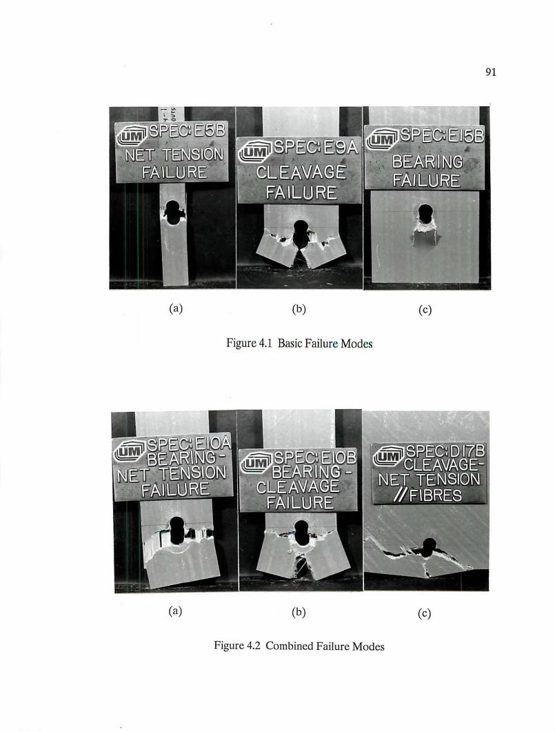
91

(a) (b) (c)

Figure 4.1 Basic Failure Modes

(a) (b) (c)

Figure 4.2 Combined Failure Modes

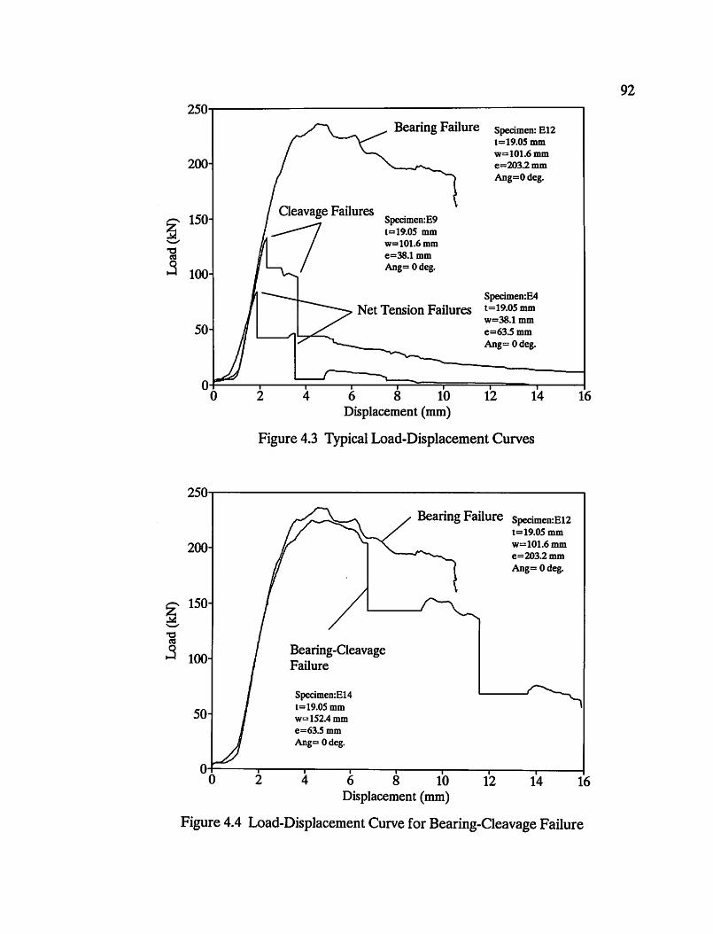
250~------------------------------------~

200

Specimen: E12 t=19.05 mm w=101.6mm e=203.2mm Ang=Odeg.

~ 150

-g

Specimen:E9 t=19.05 mm w=101.6mm e=38.1 mm Ang= Odeg. .3

~ '-" "'0 ~

.3

Specimen:E4

Net Tension Failures t=19.05 mm w=38.1 mm

50 e=63.5mm Ang= Odeg.

O~~~---=~~~--~~==~===T=---'---~ o 2 4 6 8 10 12 14 16

Displacement (mm)

Figure 4.3 Typical Load-Displacement Curves

250

Bearing Failure Specimen:E12 t=19.05 mm

200 w=101.6mm e=203.2mm Ang= Odeg.

150

Bearing-Cleavage 100 Failure

Specimen:E14

50 t=19.05 mm w=152.4mm e=63.5mm Ang= Odeg.

0 0 2 4 6 8 10 12 14 16

Displacement (mm)

Figure 4.4 Load-Displacement Curve for Bearing-Cleavage Failure

92

140

120

100

~ .......... "0 (U

~

40

20

0 0 1 2

Bearing-Net Tension Failure Specimen:B12

t=12.7mm w=101.6mm e=203.2mm Ang= Odeg.

Net Tension Failure

345 6 Displacement (mm)

Specimen:B8 t=127mm w=50.8mm e=101.6mm Ang= Odeg.

7 8 9

Figure 4.5 Load-Displacement Curve for Bearing-Net Tension Failure

140 Net Tension Failure Specimen:D18

t=12.7mm 120 w=254mm

e=63.5mm Ang=45deg.

100

~ 80 Cleavage-Net Tension Specimen:D17 Failure t=127mm

.......... w=254mm "0

(U e=38.1 mm ~ 60 Ang=45 deg.

40 Cleavage Failure Specimen:D16 t=12.7mm w=254mm

20 e=19.05mm Ang=45deg.

0 0 2 4 6 8 10 12 14 16

Displacement (mm)

Figure 4.6 Load-Displacement Curve for Cleavage-Net Tension Failure

93

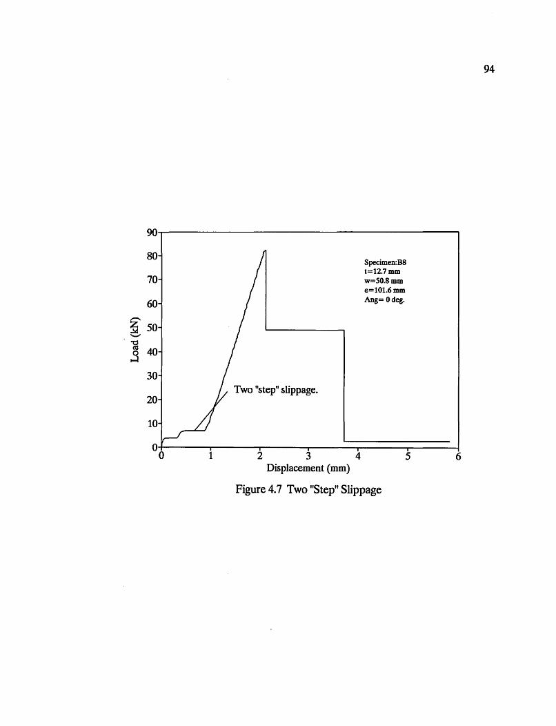
90

80

70

60

~ 50 .......... "C as 40 3

30

20

10

0 0 1

Two "step II slippage.

2 3 4 Displacement (mm)

Specimen:BS t=12.7mm w=50.Smm e=101.6mm Ang= Odeg.

5

Figure 4.7 Two "Step" Slippage

94

6

,-... fIl -~

Ja '-"

~ 0 .-

o .~ .-0 0 ~

8 fIl 0 = .-0 fIl

0

,-... ~

~ Ja '-"

~ .9

Vol .> is aJ ~

8 fIl

J3 ·0

Vol

0

225

200 ~pecirr en:A~

175

150

125

100

75

Be .

of

L ~ad Si~ ~al Fai. :Ure Ev ~nt

II 1

/ / .I.J A -... ... _ ..... ~vY' - -. ...

J ... a"'- ... _ ....... .a ... ..... ... .. ................... 1 ..

50 [\

,. ,~ -. '. -- -- - ''0'' ... Di ~placel !lent Si ~al

25 0 0.1 0.2 0.3 0.4 0.5 0.6 0.7 0.8 0.9 1 Time (sec)

Figure 4.8 Oscilloscope Data

225

200 Specin en: A"

175

150

125

100

75

50

adS gnal VI eginni pgofl ailure avent I .."...

I ~ ~

~ ~ ~ ~

"' ..,. ..r..... V

.A .l/ -- -r- -.,.

~_W 1\ VVVv \

'~isplac ement ~ignal 25

0.65 0.66 0.67 0.68 0.69 0.7 0.71 0.72 0.73 0.74 0.75 Time (sec)

Figure 4.9 Oscilloscope Data (Expanded Time Scale)

95

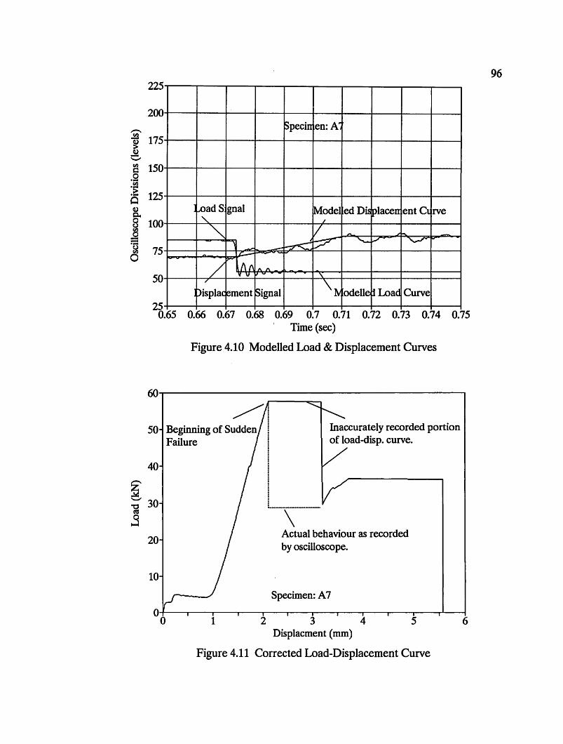
96 225

200

..-.. Specin en: A" ~ 175 ~ ~ .......... fIl 150 s:: 0 .• . ~

125 .• 0 ~ c.. 8 100 fIl

~ .• t.> 75 fIl

0

50

J..oad S gnal ~odel edDi5 placen entCl rve "- /

~ V ~ ....

~ 7 "-v '--"" I""

"' .,. -~ L..-- ..... r---

~ 1\ f\ / AI\. 'f V - '\.

/

\rv J)isplac ~ment Signal odelle ~Load Curve 25

0.65 0.66 0.67 0.68 0.69 0.7 0.71 0.72 0.73 0.74 0.75 Time (sec)

Figure 4.10 Modelled Load & Displacement Curves

60

50 Beginning of Sudden Failure

40 i

~ I :

:;- 30 i L ________

ca \ 3 20

Actual behaviour as recorded by oscilloscope.

10

Specimen: A 7

0 0 1 2 3 4 5 6

Displacment (mm)

Figure 4.11 Corrected Load-Displacement Curve

97 400

--- B e=19.0S mm ~

.......... e=38.1 mm cu ~ B

~ e=63.5mm .... --..d e=101.6mm oW -* bO = e=203.2mm ~ oW (/)

gr 200 c c ·c cu 0 ~

B cu Fibre Orientation: 0 deg. S 100 .- c oW

S NT

0 0 2 4 6 8 10 12 14

Width/Hole Diameter (wId)

Figure 4.12 Bearing Strength vs (wId) Ratio for Test Series A

400

--- B e=19.05mm ~

.......... e=38.1 mm cu ~

~ 300 e=63.5 mm -- .... ..d e=101.6mm oW -* bO c:: e=203.2mm

~ oW (/)

bO 200 c c:: c ·c ~ 0 ~ 0 oW cu Fibre Orientation: 0 deg. .5 100 oW c S

NT

0 0 2 4 6 8 10 12 14


Figure 4.13 Bearing Strength vs (wId) Ratio for Test Series B

,..., CI:S

~ --..d bo s:: ~ .... til bI)

.~ CI:S Q)

~ Q) .... CI:S

. § .... :5

400

---e=19.05mm -H- B e=38.1 mm

"'"*'" B-C 300 e=63.5mm ...

e=101.6mm ~ e=203.2mm

200 C C

100 Fibre Orientation: 0 deg .

C

NT

0 0 2 4 6 8 10 12 14

Width!Hole Diameter (wId)

Figure 4.14 Bearing Strength vs (wId) Ratio for Test Series E

400~====~--------------------------~

--e=19.05mm -H-e=38.1 mm

"'"*'" e=63.5mm ... e=101.6mm

NT

B

C

~----~~----------~C

Fibre Orientation: 0 deg.

o+-----~----~----~------~----~----~----~ o 2 4 6 8 10 12 14 WidthIHole Diameter (wId)

Figure 4.15 Bearing Strength vs (wId) Ratio for Test Series A, B, and E

98

99 200

~

e=38.1mm -... as ... ~ e=63.5mm

~ 150 ....

..r::: e=IOI.6mm

be Cl ~ ~

en c= 0 100 .-cg ~ ~

~ 0 ~

50 ~

.5 ~

:5

0 0 2 4 6 8 10 12 14


Figure 4.16 Net Tension Strength vs (wId) Ratio for Test Series A, Band E

400 .... w=2S.4mm B ~ w=38.lmm B -...

~ ... ~ 300 w=SO.8mm

~ ~

w=I01.6mm ..r::: be ~ 8-NT B-NT c= w=lS24mm

~ .... ~ w=2S4mm en b.O 200 .~ ~ ~

Fibre Orientation: 0 deg. cu JlE NT ~ NT B ~ g as .5 100 NT NT ~

:5 c

• • NT NT

0 0 2 4 6 8 10

Edge Distance/Hole Diameter (e/d)

Figure 4.17 Bearing Strength vs (e/d) Ratio for Test Series A

100 400

II

~

w=2S.4mm ~

w=38.1mm I - /~8 ".-... c:u ~

~ 300 w=SO.8mm -e-

'-" w=101.6mm ..d bo ""* I Ir ./' 8-NT c:: w=lS24mm

~ ... ...- w=2S4mm 00 ~ 200 ·c

100l /~

c:u Fibre Orientation: 0 deg. Ql

~

£ NT NT c:u ~ e .... NT NT ...-:3

~ • • NT NT

01 I I I I

0 2 4 6 8 10 Edge Distance/Hole Diameter (e/d)

Figure 4.18 Bearing Strength vs ( e/d) Ratio for Test Series B

400 ~

w=2S.4mm ~ 8 ~ w=38.1mm

¥~-~--".-...

~ c:u

~ 300 w=SO.8mm 8-NT -e-

'-" w=lOl.6mm ..r:::: bo ""* c: w=lS24mm

~ ... ...- w=2S4mm 00 ~ 200 ·c c:u

1001 !~ Nl Fibre Orientation: 0 deg. Ql

j:Q Ql ...-c:u g e NT .-...- NT :3 C ..

• • NT NT

01 I I I I


Figure 4.19 Bearing Strength vs (e/d) Ratio for Test Series E

400

---w=25.4mm -H- 8 w=38.1mm 8 ........

co "*'" ~ 300 w=SO.8mm ~ .......... w=101.6mm .d

i .... 8-NT w=254mm

~ ~

C'I') bI) 200 c ·c

m~r cu Fibre Orientation: 0 deg. Q)

~ ~ NT Q)

~ ~

co ~ e 100 .- NT NT NT ~

:5 c

• • NT NT 0

0 2 4 6 8 10 Edge DistancelHole Diameter (e/d)

Figure 4.20 Bearing Strength vs (e/d) Ratio for Test Series A, B, and E

200~----------------------------~~==~

£ co 50 e .~ :5

:

--w=25.4mm -Hw=38.1mm ~

w=SO.8mm ~

w=101.6mm

"'"* w=lS24mm

*" w=254mm

O+-~T-------~~~~--~------~--~--~--~~ o 2 4 6 8 10 12

Edge DistancelHole Diameter (e/d)

Figure 4.21 Net Tension Strength vs (e/d) Ratio for Test Series A, B, and E

101

~

~ ~

'0

'" .3

(a) (b) (c)

Figure 4.22 Effect of Fibre Orientation on Failure Mode

160

140

120

100

80

60

40

20

0 0

Figure 4.23

2 4

Specimen B14 Ang =Odeg. Cleavage Failure

Specimen D 14 Ang=45 deg. Net Tension Failure

Specimen C14 Ang= 9Odeg .

All Specimens: t=12.7 mm w=152.4 mm c=63.5 mm

Net Tension Failure

6 8 10 Displacement (mm)

12

Effect of Fibre Angle on Load-Displacement Behaviour

102

103 400

---e=19.0Smm Fibre Orientation: 45 deg. B

-H-e=38.1 mm

"'""' ~ ~

~ 300 e=63.Smm

"'-" ... ..s:= e=101.6mm ... ~ bO = e=203.2mm Q) .... ...

C'J'.) C-NT

~ 200 .-.... ~ Q)

~ Q)

Failure Mode= Net Tension ... «S

C .9 100 except were designated . ... S

O+-----~------~----~----~------~-----r----~ o 2 4 6 8 10 12 14 Width/Hole Diameter (wId)

Figure 4.24 Bearing Strength vs (wId) Ratio for Test Series D

400

---e=19.0Smm Fibre Orientation: 90 deg. -H-

B "'""'

e=38.1 mm C'CI ~

~ 300 e=63.Smm

"'-" ... ..cl e=101.6mm

bo ~

= e=203.2mm

~ ... C'J'.)

bO 200 = ·c «S Q)

~ Q) ... Failure Mode= Net Tension «S

.9 100 except were designated . ... 5 C

OT-----~------~----,_----~------r_----~----~ o 2 4 6 8 10 12 14 Width/Hole Diameter (wId)

Figure 4.25 Bearing Strength vs (wId) Ratio for Test Series C

400

--- B e=19.05mm ~

",-... e=38.1mm B-NT

(U -.-~ e=101.6mm ........,

NT ..c:I ~ s:l ~ - C en bIl 200 s:l C-NT ·c (';S

NT v j:Q 0 - NT C'CS

.8 -5 =-C

NT 11= Fibre Orientations: 0, 45, 90 deg. 0

0 2 4 6 8 10 12 14 WidthIHole Diameter (wId)

Figure 4.26 Bearing' Strength vs (wId) Ratio for Test Series B, C, and D

400T.=====~----------------------------~

",-... (U

~ 300

t -en ~ 200 .-.... B

j:Q

£ C'CS

.8 100 -5

--w=25.4mm ~

w=38.1mm ~

w=50.Smm ~

w=101.6mm

""'*" w=1524mm -.-w=254 mm C-NT

•

Fibre Orientation: 45 deg.

Failure Mode= Net Tension except were designated.

• o+---~--~----~--~--~----~--~--~----~--~ o 2 4 6 8 10

Edge DistanceIHole Diameter (e/d)

Figure 4.27 Bearing Strength vs (e/d) Ratio for Test Series D

104

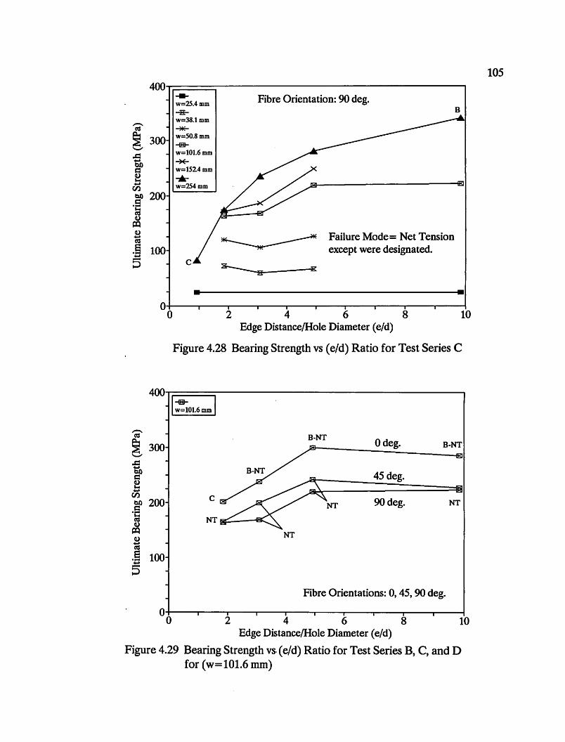
400 ... Fibre Orientation: 90 deg. w=25.4mm -H- B w=38.1mm -= -*""

:E 300 w=50.8mm ~

........." w=101.6 mm .d - ~ bI)

d w=1524mm e .... - w=254mm (J) bI) 200 c:: .;:: = Q.)

~ Q.)

Failure Mode= Net Tension -= .5 - 100 except were designated.

::5 C ~H .g

• • 0


Figure 4.28 Bearing Strength vs (e/d) Ratio for Test Series C

400T.=====~------------------------------'

"I :!i01.6 mm I "

B-NT Odeg. 1':11. B-NT -

"lQI

B-NT 45 deg.

N:~NT 1i

9Odeg. NT

NT

Fibre Orientations: 0, 45, 90 deg.

OT----.-.--,----~I--~I----~I--~~--~---~.--~--~ o 246 8 10 Edge Distance/Hole Diameter (e/d)

Figure 4.29 Bearing Strength vs· (e/d) Ratio for Test Series B, C, and D for (w=101.6 mm)

105

400~-------------------------------------------

1~2S4mm I

c

Fibre Orientations: 0, 45, 90 deg.

O+---~--~--~--~~--~------~--~--~~~ o 2 4 6 8 Edge Distance/Hole Diameter (e/d)

Figure 4.30 Bearing Strength vs (e/d) Ratio for Test Series B, C, and D for (w=254 mm)

10

106

107 8

7 - w/2 = 50.8mm -.... - -0 C)

6-tf = 5- Specimen: A21 0 .~

t=9.525mm -e - 4- w=101.6mm = 8 e=lOl.6mm = 3 8

~-=; Ang=Odeg.

= 2 .~ e -CI) 1-

0 0 i I I 2

8

7 w/2 = 76.2mm .... 0 -y

6 tf = 5 Specimen: A22 0 ..... t=9.525mm -e

w=152.4mm - 4 = 8 e=101.6mm = 3 Ang=Odeg. 8 = 2 .~

«S .... -CI) 1

0 0 1 2 3

8

7 w/2 = 127mm .... ~ 6 tf = 5 Specimen: A19 0 .....

t=9.525mm -. e - 4 w=254mm = 8 e=101.6mm = 3 8 Ang=Odeg. .9 2 e -CIl

1

0 0 1 2 3 4 5 6

Gauge Location/Hole Diameter (x/d)

Figure 4.31 Effect of Width on SCF for Material Thickness t=9.525 mm

108 8

7 w/2 = 50.8mm .... ~ 6 d! = 5 Specimen: Ell .9 - t=19.05mm e - 4 w=101.6mm = 8 e=101.6 nun = 3 8 Ang=Odeg.

= .• e -fJ'.)

1

0 0 1 2

8

w/2 = 76.2mm .... 0 0 d! = 5 Specimen: E15 0 .•

t=19.05nun -e - 4 w=152.4mm = 8 e=101.6mm = 3 8 Ang=Odeg.

= 2 'f -fJ'.) 1

0 0 1 2 3

8

7 w/2 = 127mm .... 0 -CJ 6 tf = 5 Specimen: E19 0 .•

t=19.05 nun -e - 4 w=254mm = 8 e=101.6mm = 3 8 Ang=Odeg.

= 2 .• ~ .... -fJ'.)

1

0 0 1 2 3 4 5 6

Gauge Location/Hoie Diameter (x/d)

Figure 4.32 Effect of Width on SCF for Material Thickness t= 19.05 mm

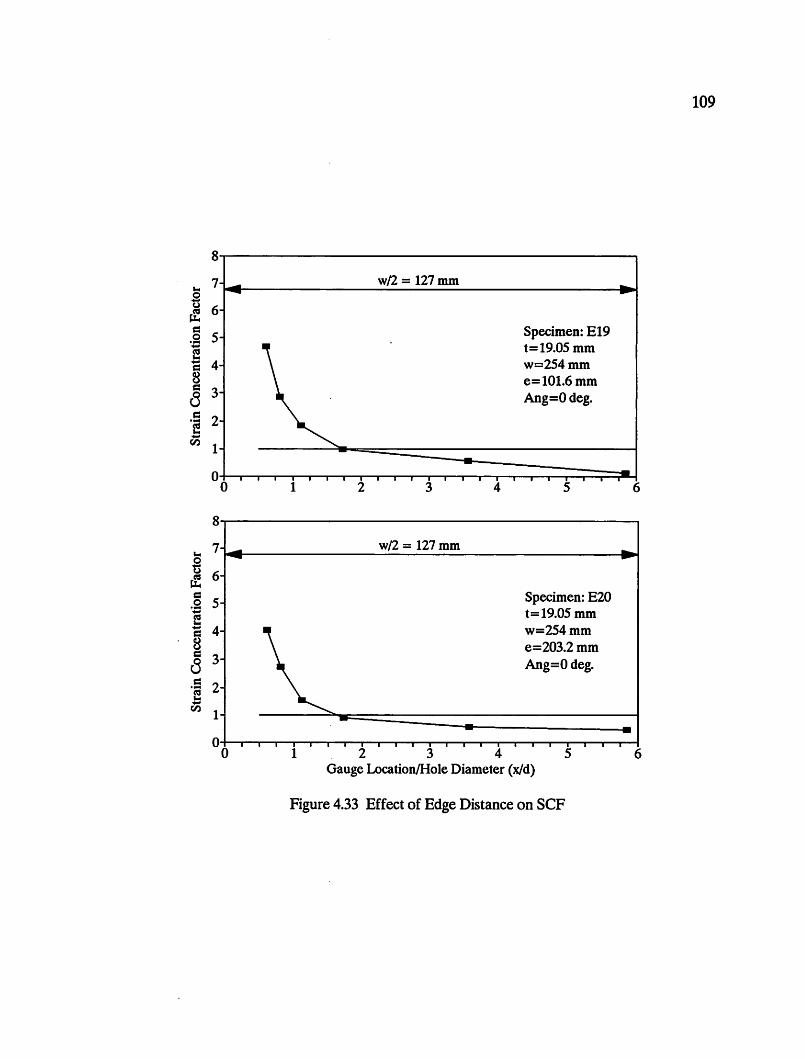
109

8

7 w/2 = 127mm ... 0 ts 6 d! = 5 Specimen: E19 0 ....

t=19.0Smm -(U ... w=2S4mm - 4 = 8 e=lOl.6mm = 3 8 Ang=Odeg.

= 2 .... e -CI) 1

0 0 1 2 3 4 5 6

8

7- - w/2 = 127mm -... - -0 ts 6-d! c:I

5- Specimen: E20 .9 - t=19.0S mm e - 4- w=2S4mm = 8 e=203.2mm c:I 3-8 Ang=Odeg. c:I 2-.... e -CI)

1----

0 . . .. I I I 4. • I I

0 1 2 3 5 6 Gauge LocationlHole Diameter (x/d)

Figure 4.33 Effect of Edge Distance on SCF

110 8

7 w/2 = 127mm ... ~ 6 tf = 5 Specimen: A19 0 .....

t=9.525mm -e - 4 w=254mm

~ e=101.6mm

8 3 Ang=Odeg . . S 2 e -en

1

0 0 1 2 3 4 5 6

8

7 w/2 = 127mm ... 0 -u 6 tf = 5 Specimen: B19 .9 - t=12.7mm e - 4 w=254mm 8 e=101.6mm = 3 8 Ang=Odeg. c:I 2 ..... e -en

1

0 0 1 2 3 4 5 6

8

7- - w/2 = 127mm -... - -0 -u 6-~ c:I

5- Specimen: E19 .9 - t=19.05 mm e - 4- w=254mm = 8 e=101.6mm = 3 8 Ang=Odeg.

= 2 ..... e -en 1-

0 · i :3 · I 4 I 0 1 5 6 Gauge LocationlHole Diameter (x/d)

Figure 4.34 Effect of Thickness on SCF

111 8

7 w/2 = 127mm ... 0 U 6 ~ d

5 Specimen: B19 0 ..... t=12.7mm -e - 4 w=254mm § e=101.6mm

8 3 Ang=Odeg.

.5 2 e -Cf.) 1

0 3 4 5 6 0 1 2

8

7 w/2 = 76.2mm ... 0 -to)

6 ~ d

5 Specimen: C15

.9 - t=12.7mm ~ ... w=152.4mm - 4 d

8 e=101.6mm d 3 Ang= 9Odeg. 8 d 2 ·e -Cf.)

1

0 0 1 2 3

8

7 w!2= 127mm

... 0 U 6 ~ d

5 Specimen: C19 0 ..... t=12.7mm -e - w=254mm d

8 e=101.6mm d 3 8 Ang= 9Odeg. d 2 ·e -Cf.)

1

0 0 1 2 3 4 5 6

Gauge Location/Hole Diameter (x/d)

Figure 4.35 Effect of Fibre Orientation on SCF

CHAPTER 5 DESIGN PROCEDURE

5.1 INTRODUCTION

This chapter discusses an analytical model proposed to descnbe the behaviour

of double-shear single-bolted connections in a fibre-reinforced composite material

in terms of the ultimate load capacity and the mode of failure. The model is semi

empirical, consisting of two basic failure criteria to determine the ultimate capacity

and failure mode of a connection.

The first criterion used in the model describes the net tension failure mode

of the connection. Prediction of the ultimate tensile strength is based on a modified

version of the theory presented by Hart-Smith (39). The theory accounts for the

elastic stress concentrations at a loaded hole in an elastic, isotropic material. For

fibre-reinforced composite material, Hart-Smith introduced a correlation coefficient

which can be derived from experimental tests. This correlation coefficient relates

the elastic stress concentration factor which occurs in elastic materials to that which

occurs in fibre-reinforced composite materials for a connection of the same

geometry. The correlation coefficient accounts for the composite's orthotropy,

pseudo-yielding capability, heterogeneity, and other factors which influence the

behaviour of a bolted connection. Since the theory is based on elastic isotropic

materials, it can be applied to many material systems and fibre patterns using only

limited test data for the specific composite material. Once the correlation

112

113

coefficient for a specific system is established, the ultimate net tension load can be

predicted for any geometry.

The second criterion used in the model describes the bearing failure mode of

a bolted connection. Prediction of the ultimate bearing capacity of a connection is

based on the bearing strength of the material which can be determined from

experimental results. In the propos~d model, cleavage failure is treated as a special

type of bearing failure with an inadequate edge distance. Since the shearout mode

of failure was not obtained in the experimental part of this investigation, it will not

be extensively discussed and will be considered in future research work.

5.2 EFFICIENCY OF THE CONNECTION

The structural efficiency of a bolted connection can be defined as:

p Efficiency _ uil

tw-F III

(5.1)

where P ult is the ultimate load of the connection and t and ware the thickness and

width respectively. FlU is the unnotched tensile strength of the material. Due to the

presence of the hole, the ultimate strength of a member in a bolted connection will

obviously be less than that of a similar member without a hole, and therefore the

range of the efficiency will always be between 0 and 1.

114

5.3 NET TENSION FAILURE

The maximum stress, U max' adjacent to a bolt hole along a net section of a

member subjected to an applied load, P, perpendicular to the net section, can be

determined as follows:

U - k max Ie

p (5.2) t(w-d)

where t, w, and d are the thickness, width and hole diameter of the connection

respectively, as shown in Fig. 5.1. The elastic stress concentration factor, kte,

corresponds to the maximum stress adjacent to the hole.

The elastic stress concentration factor, k.e' for an isotropic, perfectly elastic

material, can be determined using an expression proposed by Hart-Smith (39) as

follows:

(wId-I) k - 2+(wld-1)-1.5 8

Ie (wId + 1) (5.3)

where 8 is a non-dimensional factor and is a function of the edge distance to width

ratio (e/w) as given by:

8-1.5-0.5 elw

8-1

for elwsl

for e/w?!1 (5.4)

Equations (5.3) and (5.4) were developed based on experimental data and

theoretical deductions from several sources as described in detail by Hart-Smith

(39). Equations (5.3) and (5.4) were derived so as to produce a monotonic function

in terms of the ratios (d/w) and (e/w).

115

Based on the limited number of specimens tested in this program, the test

results suggest that the limiting value of 8=1 when (e/w)~1 in Eq.(5.4) may not be

valid for the material used in this investigation. This is evident from the fact that

the ultimate average net stress of the connections tend to increase with an increasing

(e/w) ratio even past the value of (e/w) = 1 as shown in Fig. 5.2. Therefore Eq.(5.4)

originally proposed by Hart-Smith is modified for the proposed model in this

investigation to:

8 _ 1.5- 0.5 e/w

for O~e/w (5.5)

For a perfectly elastic material, when the maximum induced stress Umax reaches

the tensile strength of the material Ftu' net tension failure occurs as the crack

catastrophically propagates through the net section. The failure mode in this case

is brittle and sudden. Therefore by rearranging Eq.(5.2) and replacing the maximum

stress U max by the ultimate tensile strength of the elastic material Ftu' the ultimate

load of the connection can 'be determined as follows:

(5.6)

From Eq.(5.1) and (5.6), the efficiency of the connection can be shown to be:

Efficiency ... ~ (l-d/w) kit!

(5.7)

116

For a perfectly plastic material where the material can yield extensively before

failure, the stress concentration factor kte could eventually reach unity and Eq.(5.7)

will be reduced to:

Efficiency - (l-d/w) (5.8)

Equations (5.7) and (5.8) are plotted versus the ratio (d/w) in Fig. 5.3 for a constant

value of (e/w) = 1. It should be noted that values of (d/w) outside the interval 0 to

1 are not possible.

In Fig. 5.3 as (d/w) approaches 1, the member width approaches the size of

the hole diameter, and therefore, the efficiency of the connections will certainly

approach zero for both elastic and plastic materials. By increasing the member

width with respect to the hole diameter, that is, by decreasing the (d/w) ratio, the

efficiencies increase for both types of material. For a perfectly plastic materia~

which can yield extensively before failure, the stresses will be uniform at the net

section as shown in Fig. 5 .4( a). The stress concentration factor kte is unity and

therefore the efficiency will approach one as the (d/w) ratio approaches zero as

shown in Fig. 5.3. For a perfectly elastic material, the stress concentration factor

at the bolt hole k.e' as described by Eq.(5.7), will approach infinity as shown in Fig.

5.4(b). Therefore for a perfectly elastic material the efficiency will approach zero

as the (d/w) ratio approaches zero. The maximum efficiency that could be achieved

for a connection of a perfectly elastic material is 0.21 at (d/w) =0.4 as reported by

Hart-Smith (39).

Fibre-reinforced composites do not have the yielding capability of a ductile

117

metal, and therefore do not behave like a perfectly plastic material. However, since

composite materials still exhibit some stress concentration relief in the form of

matrix cracking, fibre-matrix debonding, fibre breakage and fibre pull-out, they do

not behave like a perfectly elastic material either. Therefore, the behaviour of

bolted connections in fibre-reinforced composite materials is neither fully plastic nor

fully elastic but somewhere in between as shown in Fig 5.3.

Since bolted connections in fibre-reinforced composites exhibit some stress

redistribution before ultimate failure, the stress concentration factor kte, for isotropic

perfectly elastic materials, is too high for fibre-reinforced composites, and therefore

it predicts an efficiency that is too low. To correlate the two materials, it has been

reasonably shown that the stress concentration factor in isotropic elastic materials

kte, and those in fibre-reinforced composites ktc are linearly related and can be

expressed in terms of a correlation coefficient, C, by the following equation given

by Hart-Smith (39):

(5.9)

where:

k _ F t(w-d) Ie tu p

uII

(5.10)

Ftu is the ultimate tensile strength of the composite material in the loaded direction,

and P ult is the ultimate load of a composite connection. The term ktc is the average

stress concentration factor observed at failure of a bolted connection using

composite material members and kte is the corresponding elastic stress concentration

118

factor of a connection with the same geometry using a perfectly elastic isotropic

material. Computing kte for perfectly elastic isotropic materials, and ktc from

Eq.(5.10) based on measured experimental values, the correlation coefficient C can

be determined for any fibre-reinforced composite material using a limited number

of experimental observations. The correlation coefficient, C, accounts for the

composite's orthotropy, pseudo-yielding capability, heterogeneity, clearance effects,

and other factors which affect the behaviour of bolted connections. It should be

noted that the linear relationship in Eq.(5.9) is valid only for the net tension mode

of failure and therefore only experimental results for connections that failed in net

tension should be used to determine the correlation coefficient.

In this investigation three different fibre orientations were used. The

connections were tested with the applied load at 0°, 45°, and 90° to the

unidirectional fibre layers. The measured results were used to determine the

correlation coefficient for the 0°, 45°, and 90° fibre orientations, based on a least

squares regression analysis as shown in Fig. 5.5, Fig. 5.6, and Fig. 5.7 respectively.

For this analysis, values of ihe composite stress concentration factor k.c were based

on Eq.(5.10) and the values of k.e were based on Eq.(5.3) for the same connection

geometry. In these figures the correlation coefficient C represents the slope of the

best-fit-straight line. Due to the nature of Eq.(5.9) the best-fit-curve is constrained

by the point (1,1). The correlation coefficients for the fibre orientations of 0°, 45°,

and 90° to the applied load were found to be 0.33, 0.21 and 0.25 respectively for

EXTREN Flat Sheet! Series 500. The standard errors of the correlation coefficients

119

as determined from the regression analysis were 0.0153, 0.096, and 0.0307

respectively. The correlation coefficient for the 45° fibre orientation connections is

the lower than the 90° case, since the lowest tensile modulus occurs approximately

at 45° to the unidirectional fibres as discussed in Chapter 3.

Using the stress concentration factor k.c and Eq.(5.7), the efficiency of a

single-bolted connection in a fibre-reinforced composite can be expressed as:

Efficiency - ~ (l-d/w) k,c

(S.ll)

Equation (5.11) can be expressed in terms of C and k.e as:

Efficiency - 1 (l-d/w) C(k,e -1)+1

(5.12)

Consequently, the ultimate load of a single-bolted connection in a composite

material can be determined using Eq.(5.1) as follows:

(5.13)

Therefore, for a given correlation coefficient C and the tensile strength of a

composite material, the design engineer can predict the ultimate "net tension failure"

load of a single-bolt connection, of any geometry using Eq.(5.13).

Equation (5.12) was used to produce a family of failure envelopes in terms of

the connection's efficiency and the ratio (d/w) as shown in Fig. 5.8 to Fig. 5.10 for

the three fibre orientations used in this investigation. Each envelope in Fig. 5.8 to

5.10 is given for a constant (e/d) ratio. As can be seen, the failure envelopes predict

the test results extremely well. The experimental results indicated in general that

120

connection strengths increased by increasing the edge-distance up to a maximum

value of (e/d)=5. Therefore, the failure envelope corresponding to (e/d)=5 is set

as the outermost failure envelope.

5.4 BEARING/CLEAVAGE FAILURE

As (d/w) approaches zero, the connection becomes infinitely wide with respect

to the hole diameter and net tension failure is preceded by bearing failure for

connections with large edge distances and by cleavage or shearout failure for

connections with small edge distances. The ultimate bearing capacity of a

connection is obviously dependent on the bearing strength of the material. Using

the results of a full size connections, the bearing strength of a material Fbr can be

determined as:

(5.14)

where dbolt is the diameter of the bolt. The hole diameter, d, used in this

investigation was 20.6 mm (13/16 in.) and the bolt diameter, dbo1l' was 19 mm (3/4

in.).

The bearing strength of fibre-reinforced composite materials can be

determined using a standard test, ASTM Standard D953. However, measured

results could be very conservative compared to the bearing strength of actual full

size connections. Therefore, it is recommended to use full size connections to

determine the actual bearing strength.

121

The efficiency of a connection that fails in bearing, can be expressed in terms

of the ratios Fb/Ftu and dbo1ld as:

F d d Efficiency - ~ ~ -

Fru d W

(5.15)

Equation (5.15) is presented in Fig. 5.11 for the case of d=dbolt and various Fb/Ftu

ratios. The term (Fb/Ftu)( dbo1ld) is equivalent to the slope of the lines shown in

Fig. 5.11.

In this investigation it was found that increasing (e/d) ratios did not increase

the bearing stresses appreciably for (e/d)~5 as shown in Fig 4.20 and repeated in

Fig. 5.12. The failure for these connections was predominantly bearing failure,

therefore all connections that had (e/d)~5 were used to determine the material

bearing strength, Fbrt for the three fibre orientations used in this investigation.

Using Eq.(5.15), Fig. 5.13 to Fig. 5.15 illustrate the best-fit lines for the three fibre

orientations considered using a least squares regression analysis. From the test

results of the connections with the specified bolt diameter to hole diameter ratio,

the bearing strength to tensile strength ratios, Fb/Ftu, were found to be 1.84, 2.20,

and 2.13 for the 0°, 45°, and 90° fibre orientations respectively. The numerical

values are given for the three fibre orientations in Table 5.1. Using Eq.(5.14), the

average value and standard deviation of the Fb.fFtu ratios of the specimens with

(e/d)~5 are given in Fig. 5.16 to Fig. 5.18 for the three fiber orientations. The

average Fb/Ftu values are 1.95, 2.51, and 2.38 for the 0°, 45°, and 90° fibre

orientations respectively. As can be seen from Table 5.1 the average value of Fbr as

122

determined from Eq.(5.14) is slightly higher than the least squares value of Fbr as

determined from Eq.(5.15). The large standard deviations as given in Table 5.1 are

possibly due to the large material variability as well as the influence of combined

modes of failure for those connections near the transition zones of the failure

modes. The values obtained by the least squares method based on Eq.(5.15) were

used in this investigation.

It should be noted that for a given (d/w) ratio and for adequate edge

distances, the predominant mode of failure is bearing. With a decreasing (e/d) ratio

the mode of failure tends to change from bearing failure to cleavage failure. In this

investigation it was found that cleavage failure is related to bearing failure by a

simple quadratic expression in terms of the ratio (d/2e). This expression is a

reduction factor that relates the efficiency of a connection that would tend to fail

in bearing to the efficiency of a similar connection with a smaller edge distance that

would tend to fail in cleavage and is expressed as:

Cleavage Reduction Factor - (1_~)2 2e

(5.16)

The quadratic expression was found to be the simplest and fit the measured

data the best. By introducing this reduction factor into Eq.(5.15) an expression that

characterizes both bearing and cleavage failure can be defined as follows:

(5.17)

123

Equation (5.17) satisfies the limiting case as (e/d) approaches 00, as the

quadratic term in Eq.(5.17) becomes unity and the efficiency reduces to Eq.(5.15)

given before for bearing failure. Equation (5.17) satisfies the other limiting case

which occurs when (e/d) approaches 1/2, and the expression predicts zero capacity

of the connection. This is due to the fact that "e", which is measured to the centre

of the bolt hole, cannot be less than half the hole diameter.

The results of this investigation show that for connections with (e/d)~5 the

failure mode is predominantly bearing. Therefore to satisfy this new practical limit,

the cleavage reduction factor should reduce to 1 when (e/d)=5. To accomplish this,

the constants in the cleavage reduction factor must be computed based on the

practical boundary conditions. Equation (5.17) can be rewritten in terms of constant

coefficients "a" and "b" as follows:

F d d d Efficiency - ~ ~ (a-b_)2 _

Fa, dew

Therefore to satisfy the upper limit when (e/d)=5:

b (a--) - 1

5

and to satisfy the lower limit when (e/d) = 1/2:

(a-2b) - 0

(5.18)

(5.19)

(5.20)

124

Solving Eq.(5.19) and (5.20) simultaneously, the two constant coefficients were

found to be: a= 10/9 and b=5/9.

Therefore, for (e/d)s5 Eq.(5.18) becomes as follows for cleavage failure:

. F br dOO11 10 5 d)2 d fi (U) 5 Efficiency - - - (---- - or e,u S Fill d 9 9 e w

Cleavage (5.21)

For (e/d)~5 Eq.(5.18) reduces to Eq.(5.15) for bearing failure:

. Fbr dOOIl d Efficiency - - - -

Fill d w for(e/d)~5 Bearing (5.22)

Using the least efficiency, the ultimate load of a connection can be determined as:

P utI - Efficiency (t· w· Fill) (5.23)

Equations (5.21) and (5.22) were used to produce a family of failure envelopes

in terms of the efficiency and the ratio (d/w) as shown in Fig. 5.19 to Fig. 5.21 for

the three orientations used in this investigation. The various envelopes are given for

constant (e/d) ratios. The cUlVes are in excellent agreement with the measured

experimental values for both bearing and cleavage modes of failure.

The shear-out mode of failure was not obselVed in this experimental

investigation due to the presence of a high volume of random fibres in the material

used. However, since shearout and cleavage can be considered types of bearing

failures with inadequate edge distances, it is reasonable to assume that the behaviour

for cleavage failure discussed here could be applicable to shearout failure which

could occur in other types of composite materials.

125

5.5 DESIGN PROCEDURE

Superimposing the failure envelopes of the two failure criteria descnoed

before, one set of design envelopes was developed for each fibre orientation as

shown in Fig. 5.22 to Fig. 5.24. Given a particular connection geometry t, w, e, d,

and dbolt the efficiency and mode of failure of the connection can be predicted using

the proposed failure envelopes for the corresponding (d/w) and (e/d) ratios and the

given fibre orientation. The efficiency can also be determined using Eq.(5.12) for

net tension failure and Eq.(5.21) or Eq.(5.22) for cleavage/bearing failure with the

lowest value of the two failure criteria determining the connection's efficiency and

its corresponding failure mode.

It can be seen that for fibre reinforced composites an optimum value of (d/w)

exists which will produce a maximum connection efficiency. For EXTREN Flat

Sheet/ Series 500 this maximum connection efficiency is approximately 0.4 for

(d/w)=O.3 and (e/d)=5. To prevent a catastrophic failure mode such as net tension,

it may be necessary to increase the width to induce bearing failure and accept a loss

in connection efficiency.

In general for any composite material, the proposed design procedure can be

used by determining the material properties and correlation coefficient

experimentally and by developing failure envelopes similar to the one used in this

investigation to predict the load capacity and the mode of failure.

The measured ultimate loads of the connections tested in this program for the

three fibre orientations are compared to the predicted values obtained from the

126

proposed design procedure in Fig. 5.25 to Fig. 5.27. The comparison indicates that

most of the data fall close to the 1:1 correspondence line or are on the conselVative

side.

Table 5.2 lists the percent difference between the measured and predicted

ultimate loads and compares the predicted mode of failure to the obselVed modes.

As the results indicate, the proposed design procedure predicted the ultimate load

and failure mode of the tested connections with an adequate degree of accuracy.

On average, the predicted loads were within 10% of the experimentally determined

values. For the 0° connections the correspondence between the predicted and

experimental failure modes was excellent with only a few discrepancies occurring for

those connections that had failed in a combined failure mode. Since the model is

based on the 0° connections, in terms of failure modes, it could not predict the

suppression of the cleavage failure mode for the 45° and 90° connections as shown

in Table 5.2. Although it had predicted the net tension and bearing failure modes

for those "angled" connections that had the same failure mode as their 0°

counterparts, it had predicted typical bearing and cleavage failure modes for those

connections in which the "angled" fibre orientation induced a net tension failure.

This is not a major problem as the prediction of failure modes can be empirically

corrected for the 45° and 90° cases.

Obviously connections that were tested with the principal fibre direction at 45°

and 90° to the applied load had lower ultimate loads than their 0° counterparts.

However, due to the lower values of FlU in these directions, their efficiencies were

127

actually higher than their 00 counterparts as shown in Fig. 5.22 to Fig. 5.24. This

means that the failure envelopes for the 00 case can also be used to predict

conservatively the loads of connections of all fibre orientations considered in this

investigation. This suggests that only one set of design envelopes needs to be used

to predict the connection behaviour regardless of the direction in which the bolt is

bearing with respect to the fibre orientation.

Because the procedure is based on isotropic theory and uses empirical data

to correlate the failure criteria it could be used for a variety of different composite

material systems. The correlation coefficient which relates the isotropic theory to

composite materials accounts for material orthotropy, pseudo-yielding capability,

hole size and clearance effects. In some respects the coefficient can be thought of

as a "catch all" factor accounting for all those effects which complicate the stress

analysis of a loaded bolt-hole. It is therefore reasonable to expect that as the

material systems and connection configurations used by civil engineers become more

standardized, a data base of test results could be developed to allow the design

engineer to "pick and choose" the appropriate "C" value from a design code without

ever doing a single test. Considering the versatility and simplicity of this design

procedure it is ideal for implementation in future design codes.

128

5.6 PRACTICAL APPLICATION

Given a connection made from EXTREN Flat Sheet /Series 500 with the

dimensions w=130 mm, e=40 mm, t=12 mm, d=21 mm, dbolt=19 mm and the

material property Ftu= 166 MPa, the structural efficiency can be determined from the

envelopes in Fig. 5.22 for (d/w)=0.16 and (e/d)=:=2 and is found to be 0.185.

Consequently the ultimate load Pult=Efficiency·t'W·Ftu is equal to 48 kN. Since the

failure is located within the straight line portion of the envelope, the failure is a

bearing or cleavage failure. In this case the failure is cleavage, since (e/d)<5.

The same results can be obtained using Eq.(5.12) and (5.21) with a correlation

factor of C=0.33 and Fbr= 1.84 Ftu' determined experimentally for this type of

material. The expression for net tension failure Eq.(5.12) gives an efficiency of 0.27

and a Pull (net tension)=70 kN while expression (5.21) gives an efficiency of 0.18 and

a Pult (cleavage)=47 kN. Since Eq.(5.21) is critical the failure mode is cleavage .

. By increasing the edge distance of the previous connection, the mode of

failure can be changed from cleavage failure to a more desirable bearing failure.

Setting e=110 mm so that (e/d)=5.2, the efficiency can be determined from Fig.

5.22 to be 0.28 and Pu1t =72 kN. Since (e/d)~5 the mode of failure will be bearing.

Using Eq.(5.12) and (5.22) the net tension efficiency can be determined to be 0.31

and Pull (net tension)=80 kN, while the bearing efficiency is found to be 0.27 and

Pub (bearing)=70 kN similar to that obtained from Fig. 5.22. Obviously bearing

failure is critical.

If a similar connection is used except with w=40 mm and e=40 mm and thus

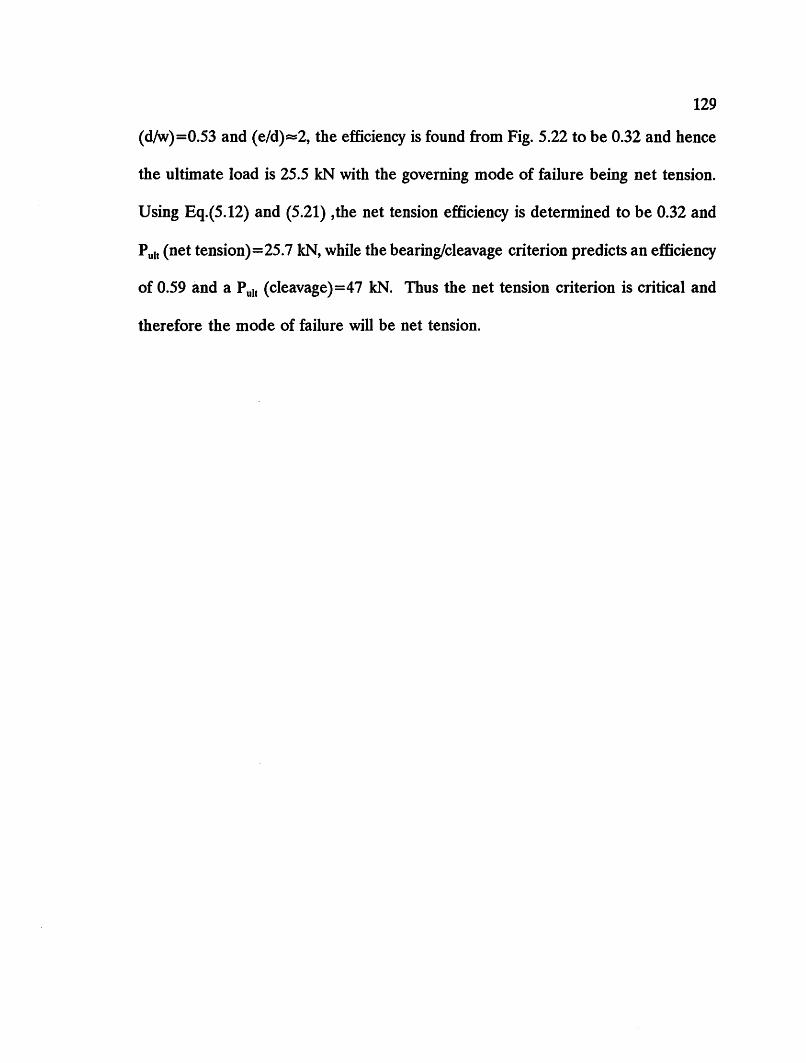
129

(d/w)=0.53 and (e/d)=2, the efficiency is found from Fig. 5.22 to be 0.32 and hence

the ultimate load is 25.5 kN with the governing mode of failure being net tension.

Using Eq.(5.12) and (5.21) ,the net tension efficiency is determined to be 0.32 and

Pull (net tension) =25.7 kN, while the bearing/cleavage criterion predicts an efficiency

of 0.59 and a Pull (cleavage)=47 kN. Thus the net tension criterion is critical and

therefore the mode of failure will be net tension.

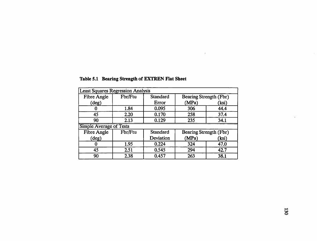
Table 5.1 Bearing Strength of EXTREN Flat Sheet

Least Squares Regression Analvsis FihreAngle Fbr/Ftu Standard Bearing Strength (Fbr)

(deg) Error (MPa) (ksi) 0 1.84 0.095 306 44.4 45 2.20 0.170 258 37.4 90 2.13 0.129 235 34.1

Simple Average of Tests FihreAngle Fbr/Ftu Standard Bearing Strength (Fbr)

(deg) Deviation (MPa) (ksi) 0 1.95 0.224 324 47.0 45 2.51 0.545 294 42.7 90 2.38 0.457 263 38.1

Table 5.2 Model Results

Test Experimental Predicted % Difference Experimental Predicted Designation Ultimate Load Ultimate Load Failure Mode Failure Mode

leN (Ibs) leN (Ibs) Plate A I Plate 8 Series A I

Al 12.2 2750 13.2 2963 7.8 NT NT NT A2 145 3250 135 302S -6.9 NT NT NT A3 44.0 9900 37.9 8511 -14.0 NT NT NT A4 43.8 9850 38.6 8685 -11.8 NT NT NT AS 39.4 8850 39.1 8787 -0.7 NT NT NT A6 55.3 12425 58.4 13125 5.6 NT NT NT A7 57.8 12990 60.4 13586 4.6 NT NT NT AS 61.3 13775 61.6 13860 0.6 NT NT NT A9 69.2 15550 73.0 16404 55 C C C A10 95.3 21425 96.3 21641 1.0 8-NT 8-NT C All 103.0 23150 111.2 24991 8.0 8-NT 8-NT 8 A12 1005 22600 111.2 24991 10.6 8-NT 8-NT 8 A13 67.6 15200 73.0 16404 7.9 C C C A14 109.4 24600 96.3 21641 -12.0 C C C A15 129.0 29000 111.2 24991 -13.8 8-NT 8 8

A16 28.9 6500 28.8 6481 -0.3 C C C

A17 66.7 15000 73.0 16404 9.4 C C C

A18 113.0 25400 96.3 21641 -14.8 C C C

A19 116.8 26250 111.2 24991 -4.8 8 8 8

A20 113.9 25600 111.2 24991 -2.4 8 8 8

A21 92.1 20700 111.2 24991 20.7 8 8-NT 8

A22 122.8 27600 111.2 24991 -95 8 8 8

Series 8

81 13.3 3000 14.8 3318 10.6 NT NT NT

82 14.9 3350 15.1 3387 1.1 NT NT NT

83 52.3 11750 505 11348 -3.4 NT NT NT

84 60.5 13600 51.5 11581 -14.8 NT NT NT

85 54.9 12350 52.1 11716 -5.1 NT NT NT

86 72.9 16400 77.8 17500 6.7 NT NT NT

87 75.4 16950 80.6 18115 6.9 NT NT NT

88 83.4 18750 82.2 18480 -1.4 NT NT NT

89 97.5 21925 97.3 21872 -0.2 C C C

810 115.1 25870 128.3 28854 11.5 8-NT 8-NT C

811 145.0 32600 148.2 33322 22 8-NT 8-NT 8

812 137.9 31010 148.2 33322 75 8-NT 8-NT 8

813 95.2 21400 97.3 21872 2.2 C C C

814 152.6 34300 128.3 28854 -15.9 C C C

815 167.2 37600 148.2 33322 -11.4 8 8 8

816 36.6 8225 38.4 8642 5.1 C C C

817 101.1 22740 97.3 21872 -3.8 C C C

818 133.9 30100 128.3 28854 -4.1 C C C

819 184.1 41400 148.2 33322 -19.5 8-NT 8 8 820 186.0 41810 148.2 33322 -20.3 8 8 8

Failure Modes: NT=Net TensIon C=Cleavage 8=8eanng 8-NT=Combmed 8eanng-Net Tension

8-C=Combined 8earing-Cleavage C-NT=Combined Cleavage-Net Tension

131

Table 5.2 Model Results (cont'd)


kN (lbs) kN (lbs) Plate A I Plate B Series C

C1 11.8 2650 10.5 2356 -11.1 NT NT NT C2 11.7 2630 10.7 2395 -8.9 NT NT NT C3 34.9 7840 363 8162 4.1 NT NT NT C4 28.7 6450 36.9 8298 28.7 NT NT NT CS 32.1 7210 37.3 8377 16.2 NT NT NT

C6 57.8 12990 57.1 12835 -1.2 NT NT NT

C7 51.2 11500 58.8 13210 14.9 NT NT NT

C8 60.9 13690 59.7 13430 -1.9 NT NT NT

C9 78.8 17720 74.9 16848 -4.9 NT NT C

C10 81.2 18250 98.9 22226 21.8 NT NT C

C11 106.3 23890 114.2 25667 7.4 NT NT B

C12 107.7 24210 114.2 25667 6.0 NT NT B

C13 82.8 18620 74.9 16848 -9.5 NT NT C

C14 90.3 20300 98.9 22226 9.5 NT NT C

CIS 120.4 27070 114.2 25667 -5.2 NT NT B

C16 39.9 8970 29.6 6657 -25.8 C C C

C17 84.2 18940 74.9 16848 -11.0 NT NT C

C18 114.2 25670 98.9 22226 -13.4 NT NT C

C19 135.8 30530 114.2 25667 -15.9 NT NT B

C20 165.1 37120 114.2 25667 -30.9 B B B

Series D

D1 11.4 2570 11.5 2592 0.9 NT NT NT

D2 11.6 2600 11.7 2629 1.1 NT NT NT

D3 40.2 9040 40.2 9045 0.1 NT NT NT

D4 31.0 6975 40.8 9177 31.6 NT NT NT

D5 43.4 9750 41.2 9253 -5.1 NT NT NT

D6 64.9 14590 64.0 14384 -1.4 NT NT NT

D7 47.8 10750 65.6 14755 37.3 NT NT NT

D8 64.0 14390 66.6 14972 4.0 NT NT NT

D9 79.8 17930 82.0 18427 2.8 NT NT C

D10 96.5 21700 108.1 24309 12.0 NT NT C

D11 116.9 26280 124.9 28072 6.8 NT NT B

D12 109.7 24670 124.9 28072 13.8 NT NT B

D13 88.9 19990 82.0 18427 -7.8 NT NT C

D14 93.9 21100 108.1 24309 15.2 NT NT C

DIS 143.2 32190 124.9 28072 -12.8 NT NT B

D16 36.3 8150 32.4 7280 -10.7 C C C

D17 89.3 20070 82.0 18427 -8.2 NT C-NT C

018 126.8 28510 108.1 24309 -14.7 NT NT C

D19 157.6 35440 124.9 28072 -20.8 NT B-NT B

020 185.6 41730 124.9 28072 -32.7 B B B

Failure Modes: NT=Net TenSion C-Cleavage B-Beanng B-NT -Combmed Beanng-Net TenSion

B-C=Combined Bearing-Cleavage C-NT=Combined Oeavage-Net Tension

132

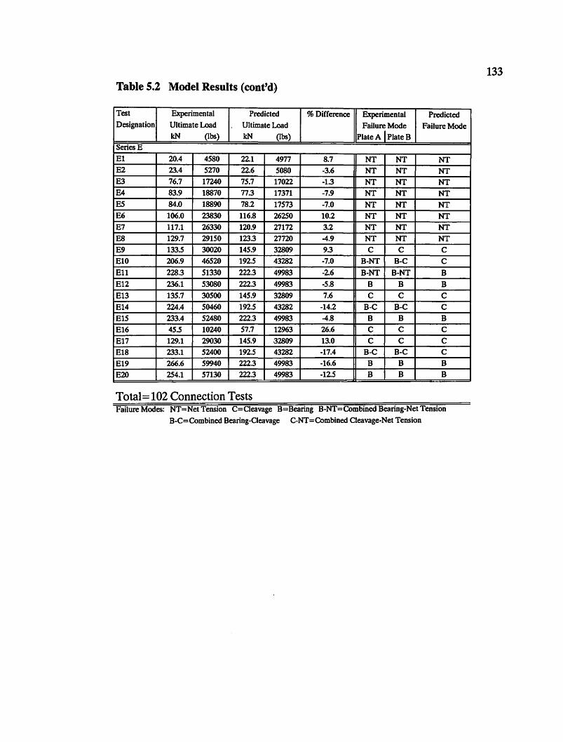
Table 5.2 Model Results (cont'd)


kN (Ibs) kN (Ibs) Plate A I Plate B Series E

El 20.4 4580 22.1 4977 8.7 NT NT NT E2 23.4 5270 22.6 5080 -3.6 NT NT NT E3 76.7 17240 75.7 17022 -1.3 NT NT NT E4 83.9 18870 77.3 17371 -7.9 NT NT NT

E5 84.0 18890 78.2 17573 -7.0 NT NT NT

E6 106.0 23830 116.8 26250 10.2 NT NT NT

E7 117.1 26330 120.9 27172 3.2 NT NT NT

E8 129.7 29150 123.3 27720 -4.9 NT NT NT

E9 133.5 30020 145.9 32809 93 C C C

EI0 206.9 46520 192.5 43282 -7.0 B-NT B-C C

Ell 228.3 51330 222.3 49983 -2.6 B-NT B-NT B

E12 236.1 53080 222.3 49983 -5.8 B B B

E13 135.7 30500 145.9 32809 7.6 C C C

E14 224.4 50460 192.5 43282 -14.2 B-C B-C C

E15 233.4 52480 222.3 49983 -4.8 B B B

E16 45.5 10240 57.7 12963 26.6 C C C

E17 129.1 29030 145.9 32809 13.0 C C C

E18 233.1 52400 192.5 43282 -17.4 B-C B-C C

E19 266.6 59940 222.3 49983 -16.6 B B B

E20 254.1 57130 222.3 49983 -12.5 B B B

Total = 102 Connection Tests Failure Modes: NT=Net Tension C=Cleavage B=Bearing B-NT=Combined Bearing-Net Tension


133

134

t

p

e

Figure 5.1 Connection Parameters

170

160

150 .--.. = ~ 140 --.--.. .--.. 130 "0

I

~ 120 ---~

rn 110 ~ -en 100 - ---w/d=1.23

~ 90

-+-w/d=1.85 ~

80 w/d=2.46

70 0 2 3 456 7 8 9

Edge Distance/Width (e/w)

Figure 5.2 Effect of (e/w) on Net Stress

0.8

= 0.7 (t: * ~ 0.6 * ~ ::::::' ~ 0.5 ~ .g 0.4 u S ~ 0.3

0.2

0.1

00

Perfectly Plastic Materials

0.1 0.2 0.3 0.4 0.5 0.6 0.7 0.8 0.9 Hole Diameter/Width (d/w)

Figure 5.3 Net Tension Failure Criteria

Perfectly Plastic Perfectly Elastic

(a) (b)

Figure 5.4 Difference in Plastic and Elastic Behaviours

135

1

136 3

• I-f--

t=9.5mm 2.5

+

~ 2 CIl

B .-en

~ 1.5

8 '-'

~ 1

'-I--- t=12.7 mm

* ..;J ~ VIc = 0.33 t=19mm

1 ..L

f1! ""

~ V'4

0.5

00 0.5 1 1.5 2 2.5 3 3.5 4 4.5 5 kte (Elastic-Isotropic SCF)

Figure 5.5 Correlation Coefficient for 0 deg. Connections

3

• 2.5 - t=12.7 mm @45deg.

G;' 2 U CI)

B .~

0 1.5 ~ a 8 '-' u 1 J;;;

~ C=( .21 .-. .... ~ 1 ~ ~. ----

0.5

00 0.5 1 1.5 2 2.5 3 3.5 4 4.5 5 kte (Elastic-Isotropic SCF)


3

2.5

~ 2 en

.~ V.I & 1.5 S -.

8 '-"

.!J 1

0.5

o

0.45

0.4

0.35 -::s a: 0.3 * ~ ~ 0.25 a:; ~ c: 0.2 (I) .-to)

0.15 S ~

0.1

0.05

0

• -f--t=12.7 mm @90deg.

-' ~ • C-O 25

~ ~ 1

~ ~ •

o 0.5 1 1.5 2 2.5 3 3.5 4 4.5 5

0

kte (Elastic-Isotropic SCF)


0.1 0.2

e/d> =5 e/d=3

• e/d=.9

+ e/d=1.8

e/d=3 o

e/d> =5

0.3 0.4 0.5 0.6 0.7 0.8 0.9 1 Hole DiameterIWidth (d/w)


137

0.5

0.45

0.4

a 0.35 ~

* ~ * ..... '-" ~ ~ (.) c::I (1)

·0 S ~

0.3

0.25

0.2

0.15

0.1

0.05

00

e/d> =5 e/d=3 •

e/d=.9 +

e/d=1.8

* e/d=3

0

e/d> =5

0.1 0.2 0.3 0.4 0.5 0.6 0.7 0.8 0.9 1 Hole Diameter/Width (d/w)


0.45

0.4

0.35 ,,-.... ::s

Ci: 0.3 * ~ ~ 0.25 ~ ~ 0.2 oCJ

= (1)

·u 0.15 S

~

0.1

0.05

00 0.1 0.2

• e/d=.9

+ e/d=1.8

e/d=3 o

e/d> =5

0.3 0.4 0.5 0.6 0.7 0.8 0.9 1 Hole Diameter/Width (d/w)


138

1~---------'---r------~--------------------~

0.9

0.8

';' 0.7 ~ * I 0.6 ....,

~ 0.5 g o 0.4 ·0

~ 0.3

0.2

0.1

0.1 0.2 0.3 0.4 0.5 0.6 0.7 0.8 0.9 1 Hole DiameterIWidth (d/w)

Figure 5.11 Bearing Criteria for Various FbrIFtu Ratios

400~------------------------------------------~ -. w=2S.4mm

-+w=38.1mm ~

w=50.8mm ~ w=101.6mm ~

w=2S4mm

•

/7'/~=~:--= ----__ 0 ___ _

• O+---~--~--~~--~--~------~~----------~ o 1 2 3 4 5 6 7 8

Edge DistanceIHole Diameter (e/d)

Figure 5.12 Effect of (e/d) on Bearing Stresses

9 10

139

0.45

0.4

0.35 ........ ::s

G:: 0.3 * ~ ~ 0.25 ~ ~ 0.2

.9:a (,)

~ 0.15

0.1

0.05

o

0.45

0.4

0.35 ........ ::s

G:: 0.3 * ~ ~ 0.25 ~

~ 0.2 .-c.J

~ 0.15

0.1

0.05

• I

I t=9.5mm ~

+ '-

t=12.7mm fil *=

II'-I--

t=19mm

7 iJl' Fb /Ftu= 1.84

" ill ~r/Ftu xd (b plt)/d ( l1ole)

II 1

o 0.1 0.2 0.3 0.4 0.5 0.6 0.7 0.8 0.9 1 Hole Diameter/Width (d/w)

Figure 5.13 Bearing Strength for 0 deg. Connections

/ 1 1 I

• /.: t=12.7 mm@45deg.

./ /

• il Fbrl1 tu=2 . 0 • I

/ IlbrlFtu xd(b blt)/d I hole)

f 1/

o 0 0.1 0.2 0.3 0.4 0.5 0.6 0.7 0.8 0.9 1 Hole Diameter/Width (d/w)


140

0.45

0.4

0.35 ~

= G:: 0.3 * ~ ~ 0.25 ii:; ~ 0.2 c: Q) ·0 5 0.15 ~

0.1

0.05

4

3.5

3

2.5

= ..... ~ 2 rf

1.5

1

0.5

0

V 1

• ). t=12.7 mm @9Odeg.

/ i

• 1/ fbr/Ft ~=2.1:

7 IIF br/Ftu xd (b plt)/d ( bole)

h i 4

0.1 0.2 0.3 0.4 0.5 0.6 0.7 0.8 0.9 Hole Diameter/Width (d/w)


+ Std. Dev. = 0.22 A-I 95 '\. vee - .

---~-;--~. • • • • • • ··-···i1-·-·---·-···-7·~··-·--·-··-·-·-··········---·--....... _ ....... _-_ .... -. __ ... _ ... __ ._ ...... _.

- Std. Dev. = 0.22

1 2 3 4 5 6 7 8 9 10 11 12 13 14 15 16 17 Specimen

Figure 5.16 Average FbrlFtu Ratio for 0 deg. Connections

141

1

4

3.5

3

2.5 ::s ...,

~ 2 tf

1.5

1

0.5

0

4

3.5

3

2.5 ::s ..., ~ 2 tf

1.5

1

0.5

0

+ Std. Dev. = 0.54

....................... _ ..... ____ ._ ................ _i_ ........................................ __ ......... ~

•

•

•

'" -Ave. - 2.51

........ -.................. -.................. -............ --···· .. ·7 .. · .. · .. ··············· ........ · .... _ .... ·-

1 2

- Std. Dev. = 0.54

3 Specimen

4 5

Figure 5.17 Average FbrIFtu Ratio for 45 deg. Connections

+ Std. Dev. = 0.46

- ..... - ........... ~-.... - .... . -----_ ..... _--_ ... -•

• • """ Ave. = 2.38

• • ·· .. · .. ················ .. · .. ·7·· .. ········ ... ········· .. ···_· ............................................................... . - Std. Dev. = 0.46

1 2 3 4 5 Specimen

Figure 5.18 Average FbrIFtu Ratio for 90 deg. Connections

142

143 0.45

• 0.4 e/d=.9

0.35 + e/d=1.8 ,,-...

=' * ~ 0.3 * e/d=3 ~ ~ 0.25 0

p:; e/d> =5 ~ 0.2 .= Q,)

'u 0.15 S

~

0.1 e/d~.9

0.05


Figure 5.19 Bearing Failure Envelopes for 0 deg. Connections

0.45

• e/d=3

e/d=.9 +

0.35 e/d=1.8 ,,-...

=' * .~ 0.3 * e/d=3 ~ ~ 0.25 0

---- e/d> =5 ~

~ 0.2 = .~ c.,)

0.15 S ~

0.1

0.05



0.45

• 0.4 e/d=.9

e/d=3 0.35

+ e/d=1.8 --::s * ~ 0.3 e/d=3 * ~

~ 0.25 0

ii; e/d> =5 ~ = Q) ·0

0.15 S ~

0.1

0.05

0.1 0.2 0.3 0.4 0.5 0.6 0.7 0.8 0.9 1 Hole Diameter!Width (d/w)


0.45-------------------------,

0.4

--::s ~ 0.3 * ~ ~ 0.25 ii; ~ 0.2 5 ·u S 0.15 ~

0.1

0.05

o • e/d=.9

+ e/d=1.8

* e/d=3

o

e/d> =5

0.1 0.2 0.3 0.4 0.5 0.6 0.7 0.8 0.9 Hole Diameter!Width (d/w)

Figure 5.22 Design Envelopes for 0 deg. Connections

1

144

0.5------------------------,

0.45 e/d>=5

0.4 e/d=4

a 0.35 ~

* } 0.3 ~

'-" ~ 0.25

~ .~ 0.2 .~ ~ ~ 0.15

0.1

0.05

• e/d=.9

+ e/d=1.8

e/d=3 o

e/d> =5

00 0.1 0.2 0.3 0.4 0.5 0.6 0.7 0.8 0.9 1 Hole Diameter/Width (d/w)


0.45

• 0.4 e/d=.9 e/d> =5

+ 0.35 e/d=4 e/d=1.8

",-..

:s * Ci: 0.3

e/d=3 * ~ ~ 0.25 0 -- e/d> =5 ~

~ 0.2 c:: 0 .-0

S 0.15 ~

0.1

0.05

00 0.1 0.2 0.3 0.4 0.5 0.6 0.7 0.8 0.9 1 Hole Diameter/Width (d/w)


145

3OO~------~------~------~-------r-------'

250 •

t=9.5 mm +

t=12.7 mm

* t=19mm

* *

= 150+-------~-------+--~~~~~~--r-----~ d C1)

·S C1)

I loo+-------~------~~~--~--------~----~

50+-----~~~----~------~-------+------~

O~------~-------+------~--------~----~ o 50 100 150 200 250 Predicted Load (kN)

Figure 5.25 Experimental vs. Model Results for 0 deg. Connections

250

• t=12.7 mm @45deg

200 ,-... • ~ ........... "'0 • (I;S 150 ~ -(I;S +-I c:l C1)

·S 100 C1)

I 50

50 100 150 200 250 Predicted Load (kN)


146

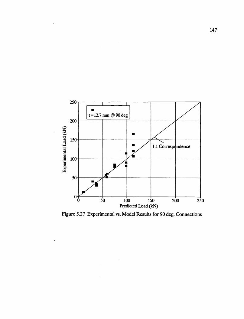
147

250

• t=12.7 mm @ 90 deg

200 ,-....

~ • "-" "0

150 ~

j • -cu -c (1.)

.~ 100 (1.)

~ 50

50 100 150 200 250 Predicted Load (kN)


CHAPTER 6 CONCLUSIONS

6.1 SUMMARY

The high strength-to-weight ratio and non-corrosion characteristics of fibre

reinforced composites makes them extremely attractive as a structural material.

However, the lack of understanding of the behaviour of advanced composite

materials has limited their acceptance and use. The structural integrity and the

capacity of buildings fabricated from fibre reinforced composite materials are mainly

controlled by the behaviour of the connections. In civil structural applications,

bolted connections are the most practical, since they are easily assembled and

disassembled, and usually cost-effective when compared to other types of

connections. Therefore an understanding of the behaviour of bolted connections is

necessary for the full potential of this material to be realized in civil structural

applications.

An experimental program was undertaken at the University of Manitoba to

investigate the behaviour of bolted connections for fibre-reinforced composite

materials. A total of 102 single-bolt double-lap connections were tested to

determine the effects of various geometric parameters on the ultimate strength and

mode of failure. In addition, an extensive material test program was conducted to

characterize the material properties and utilize them in the proposed design

procedure.

148

149

Based on the experimental results, a mathematical model and a design

procedure are proposed to predict the ultimate load and failure modes of single-bolt

connections in fibre-reinforced composite materials. The model can be applied to

other composite materials through the use of a correlation coefficient which can be

evaluated by limited test data. The procedure is simple and is ideal for

implementation in design codes.

6.2 CONCLUSIONS

Based on the obselVed and measured behaviour of 102 single-bolt connections,

the following conclusions can be made:

1. Slipping resistance is negligible at the specified bolt torque of 32.5 N-m

(24 ft-Ibs) used in this investigation.

2. Connection load-displacement behaviour is linear up to failure regardless

of the modes of failure.

3. Connections that failed in a catastrophic manner, such as in net tension

and cleavage failure, experienced a sudden drop in load canying capacity

followed by large displacements represented by a "step" in the load

displacement CUIVe.

4. For connections with a 00 fibre orientation (loaded parallel to the

unidirectional fibres), the member width-to-hole-diameter ratio (wId) had a

significant effect on the mode of failure. For relatively small edge distances

the mode of failure changed from net tension to cleavage failure by

150

increasing the (wid) ratio. For relatively large edge distances the mode of

failure changed from net tension to bearing failure by increasing the (wid)

ratio.

S. The bearing strength for connections loaded parallel to the unidirectional

fibres increased with increasing (wid) ratios up to a limiting value of (w/d)=S.

Therefore, a minimum (wid) ratio of 5 is recommended.

6. For connections loaded parallel to the unidirectional fibres with a

relatively narrow width, the mode of failure is net tension failure, regardless

of the magnitude of the edge distance. For relatively wide connections the

mode of failure changed from cleavage to bearing failure with increasing

edge distance-to-hole diameter ratios (e/d).

7. The bearing strength of connections loaded parallel to the unidirectional

fibres increased with increasing (e/d) ratios up to a limiting value of (e/d)=5.

Therefore, a minimum (e/d) ratio of 5 is recommended.

8. Increasing the thickness of the members increased the ultimate load

capacity of the connection. It was found that the member thickness had little

effect on the bearing stresses and the mode of failure. Results suggest that

high strength structural bolts, tightened to a torque of 32.S N-m (24 ft-Ibs)

as used in this investigation, were adequate to remove most of the influence

of the material thickness.

9. Connections with members having fibre orientations of 45° and 90° to the

direction of the applied load tend to be more susceptible to net tension

151

failure. Due to the transverse reinforcement of the unidirectional fibres at

angles with respect to the applied load, the cleavage mode of failure was

suppressed. Only at extreme geometric ratios could the cleavage and bearing

modes of failure be induced.

10. The bearing strengths of connections with members having fibre

orientations of 45° and 90° to the applied load tend to increase with

increasing (wid) and (e/d) ratios. Similar to the connections with fibre

orientations parallel to the applied load, the strength increases tended to

level off at values of 5 for both the (wid) and (e/d) ratios. However, to

achieve bearing failure, the results seem to indicate the minimum (wid) and

(e/d) ratios are larger.

11. The ultimate strength of connections with fibre orientations of 45° and

90° with respect to the applied load were respectively, 18% and 24% lower

than the corresponding connections with a 0° fibre orientation (parallel to the

applied load).

12. The magnitude of the stress concentrations along the net section

perpendicular to the applied load are highly influenced by the width of the

connections. The stress concentrations tend to increase with increasing

width. For relatively narrow specimens the stress concentrations adjacent to

the hole are in the order of 2 to 3 and for relatively wide connections are in

the order of 5 to 6. The member width is the dominant geometric variable

affecting the efficiency of a connection.

152

13. The effects of connection edge distance and thickness on the stress

concentrations are less than the effect of member width. Stress

concentrations tended to decrease with increasing edge distance and were

negligibly affected by the member thickness.

14. The stress concentrations seemed to increase with change in fibre

orientation from 00 to 900 with respect to the applied load.

15. The proposed design procedure predicts the ultimate load and failure

mode of the connections with an adequate degree of accuracy. On average,

the predicted loads were within 10% of the experimentally determined values.

For connections with a 00 fibre orientation, parallel to the applied load, the

correspondence between the predicted and experimental modes of failure is

excellent.

16. Because the procedure is based on isotropic theory and uses empirical

data to correlate the failure criteria it could be used for a variety of different

composite material systems.

17 Considering the versatility and simplicity of the proposed design

procedure, it is ideal for implementation in design codes.

153

6.3 RECOMMENDATIONS FOR FUTURE STUDY

1. The parametric study conducted in this investigation could be repeated,

except with intermediate values of the geometric dimensions with respect to

the ones selected in this investigation.

2. The parametric study may be extended to include more connections that

fall within the transition zones of the various failure modes to study the

behaviour of combined failure.

3. The parametric study may be extended to include the effects of other

parameters such as hole diameter, bolt diameter, clearance, bolt stiffness,

clamping force, and environmental effects.

4. The study of stress and strain distributions may be extended to include

the instrumentation of strain gauges to narrow connections, with a width less

than 100 mm (4 in.). Strain gauges may be placed at locations other than the

net section to record maximum radial strains in the bearing area around the

hole and the maximum tensile strains that occur at the free edge of the

connections where cleavage cracks initiate.

5. To help characterize the behaviour of beam-column connections, tests

may be conducted to investigate the effects of prying action and the bolt

pulling through the thickness direction of the material.

6. The experimental program may be extended to include multi-bolt

connections and effects of such factors as number of bolts per row, number

of bolts per column, bolt pattern, load bearinglbypass ratios, and stress field

154

interactions between bolt holes.

7. Combined bolted and bonded connections may be investigated to study

the general behaviour as well as the load sharing between the bolts and the

adhesive.

REFERENCES

1. Green, A., Glass-Fibre-Reinforced Composites in Building Construction. Transportation Research Record 1118, pp.73-76.

2. Sheard, P. ,1992 , Expansion of Composite Material Applications. Advanced Materials Technology International 1992 London, Sterling Publications Limited.

3. Ahmad, S.H. and Plecnik, J .M., Transfer of Composite Technology to Design and Construction of Bridges. Final Report. Prepared for u.s. Department of Transportation Federal Highway Administration. Feb. 1988.

4. Meier, U., Proposal for a Carbon Fibre Reinforced Composite Bridge Across the Straight of Gibraltar at its Narrowest Site. Proc Instn Mech Engrs, Vol. 20 1, No.B2, 1987, pp.73-78.

5. Meier, U., Topic 2 Designing and Producing Materials by Combination. Materials and Structures, Vol.21, 1988, pp.85-89.

6. Plecnik, J.M., Ballinger, E., Rao, J.K. and Ahmad, S., State-of-the-Art: Composite Materials for Bridges. Proceedings of a Workshop on Research Needs for Short and Medium-Span Bridges, Computech Engineering SeIVices, 1987, CES Report No. 5518.2, Berkeley, California.

7. Barbero, E.J., Pultruded Structural Shapes-From the Constituents to the Structural Behaviour. SAMPE Journal, Vol. 27, No.1, January/February 1991, pp.25-30.

8. Meier, U., Muller, R. and Puck, A., FRP-Box Beams Under Static and Fatigue Loading. Proceedings of the International Conference on Testing, Evaluation and Quality Control of Composite, ed. T. Feest, 1983, Butterworth, Guilord.

9. Bank, L. C., Flexural and Shear Moduli of Full-Section Fibre Reinforced Plastic (FRP) Pultruded Beams. Journal of Testing and Evaluation, JTEV A, Vol. 17, No.1, Jan., 1989, pp.40-45.

10. Bank, L.C., Properties of Pultruded Fibre Reinforced Plastic Structural Members. Transportation Research Record 1223, Bridge Design and Performance and Composite Materials, Transportation Research Board, Washington, D.C., 1989, pp. 117-124.

155

156

11. Mosallam, A.S., Short and Long-Term Behaviour of a Pultruded Fibre Reinforced Plastic Frame. PhD. Dissertation School of Engineering and Architecture, Catholic University of America, Washington, D.C., Oct., 1990.

12. Mallick, P.K,1988. Fibre-Reinforced Composites: Materials, Manufacturing, and Design. New York:Marcel Decker, Inc.

13. Cosenza, F., Mechanical Fasteners for Composites. Materials Engineering, Aug. 1987, pp.32-37.

14. Godwin, E.W. and Matthews, F.L., A Review of the Strength of Joints in Fibre-Reinforced Plastics Part 1. Mechanically Fastened Joints. Composites, July 1980, pp.155-160.

15. Bickford, J.H., Bolt Torque: Getting it Right. Machine Design, June 21, 1990, pp.67-71.

16. Bank, L.C., Mosallam, A.S., and McCoy, G.T., Design and Performance of Connections for Pultruded Frame Structures. 47th Annual Conference, Composites Institute, The Society of the Plastics Industry, Inc. February 3-6, 1992 Session 2-B pp.I-8.

17. Tsiang, T., Survey of Bolted-Joint Technology in Composite Laminates. Composite Technology Review, Vo1.6, No.2, 1984, pp.74-77.

18. Vinson, J .R., Mechanical Fastening of Polymer Composites, Polymer Engineering and Science, Mid-October, 1989, Vol. 29 No. 19, pp.1332-1339.

19. Matthews, F.L., Load Carrying Joints. Composite Materials in Aircraft Structures. D. Middleton, Ed., Longman Group UK Limited, 1990. Ch. 9. pp.142-155.

20. Bord, C., Les Materiaux Composites. CEP Edition (Editions de l'Usine nouvelle), 1983, Paris.

21. Oplinger, D.W., On the Structural Behaviour of Mechanically Fastened Joints in Composite Structures Proceedings of the Fourth Conference on Fibrous Composites in Structural Design, San Diego, California, November 14-171978, New York, Plenum Press 1980, pp.575-601.

22. Timoshenko, S.P., and Goodier, J.N., Theory of Elasticity. Third Edition, McGraw-Hill, New York, 1951, pp.90-97.

157

23. Lekhnitskii, S.G., Anisotropic Plates, Translated from the Second Russian Edition by S. W. Tsai and T. Cheron, Gordon and Breach, Science Publishers, New York, 1968.

24. Bickley, W.G., The Distribution of Stress Round a Circular Hole in a Plate, Philosophical Transactions of the Royal Society (London), Series A, Vol. 227, 1928, pp.383-415.

25. De Jong, T., Stresses Around Pin-Loaded Holes in Elastically Orthotropic or isotropic Plates, Journal of Composite Materials, Vol. 11, July, 1977, pp.313-331.

26. Collings, T.A., The Strength of Bolted Joints in Multi-Directional CFRP Laminates. Composites, Vol8, No.1, Jan. 1977, pp.43-55.

27. Kretsis, G. and Matthews, F.L., The Strength of Bolted Joints in Glass Fibre/Epoxy Laminates. Composites, April 1985.

28. Smith, P.A., Ashby, M.F., and Pascoe, K.J., Modelling Clamp-Up Effects in Composite Bolted Joints. Journal of Composite Materials, Vol 21 Oct., 1987, pp.878-897.

29. Ramkumar, R.L., Bolted Joint Design, Test Methods and Design Allowables for Fibrous Composites, ASTM STP 734, C. C. Chamis Ed., American Society for Testing and Materials, 1981, pp.376-395.

30. Tang, S., Failure of Composite Joints Under Combined Tension and Bolt Loads. Journal of Composite Materials, Vol15, July 1981, pp.329-335.

31. Agarwal, B.L., Behaviour of Multifastener Bolted Joints in Composite Materials. AIAA 18th Aerospace Sciences Meeting, Pasadena, California, Paper No. 80-0307, Jan., 1980.

32. Pyner, G.R. and Matthews, F.L., Comparison of Single and Multi-Holed Bolted Joints in Glass Fibre Reinforced Plastic. J. Composite Materials, Voll3, July 1979, pp.232-239.

33. Kim, R. Y. and Whitney, J .M., Effect of Temperature and Moisture on Pin Bearing Strength of Composite Laminates. 1. Composite Materials, Vol. 10, April 1976, pp.149-155.

158

34. Bailie, J.A., Duggan, M.F., Bradshaw, N.C. and McKenzie, T.G., Design Data for Graphite Cloth Epoxy Bolted Joints at Temperatures up to 450 K. Joining of Composite Materials, ASTM STP 749, K.T. Kedward, Ed., American Society for Testing and Materials, 1981, pp.165-180.

35. Crews, J.R., Jr., Bolt-Bearing Fatigue of a GraphitelEpoxy Laminate, Joining of Composite Materials, ASTM STP 749, K.T. Kedward, Ed., American Society for Testing and Materials, 1981, pp.131-144.

36. Tanis, C. and Poullos, M., Composite Fastener Applications for Helicopter Composite Structure Proceedings of the Fourth Conference on Fibrous Composites in Structural Design, San Diego, California, November 14-171978, New York, Plenum Press 1980, pp.652-657.

37. Chamis, C.C., Simplified Procedures for Designing Composite Bolted Joints. 43rd Annual Conference, Composites Institute, The Society of the Plastics Industry, Inc., Feb., 1988, pp.1-5 : Session 23-D.

38. Johnson, M. and Matthews, F.L., Determination of Safety Factors for Use When Designing Bolted Joints in GRP, Composites, Vol. 10, No.2, Apr. 1979, pp.73-76.

39. Hart-Smith, L.J., Mechanically-Fastened Joints for Advanced Composites -Phenomenological Considerations and Simple Analyses. Proceedings of the Fourth Conference on Fibrous Composites in Structural Design, San Diego, California, November 14-171978, New York, Plenum Press 1980, pp.543-574.

40. Hart-Smith, L.J., Joints, Composite Structures Analysis and Design, Vol. 1, 1987, pp.479-495.

41. Whitney, J.M. and Nuism er, R.J., Stress Fracture Criteria for Laminated Composites Containing Stress Concentrations. Journal of Composite Materials, Vol.8, July 1974, pp.254-265.

42. Nuismer, R.J. and Whitney, J.M., Uniaxial Failure of Composites Laminates Containing Stress Concentrations. Fracture Mechanics of Composites, ASTM STP 593, American Society for Testing and Materials, 1975, pp.117-142.

43. Waddoups, M.E., Eisenmann, J .R., and Kaminski, B.E., Macroscopic Fracture Mechanics of Advanced Composite Materials, Journal of Composite Materials, Vol.8, Oct. 1971, pp.446-454.

159

44. Pipes, R.B., Wetherhold, R.C., and Gillespie, J.W., Notched Strength of Composite Materials. Journal of Composite Materials, Vol. 13, April 1979, pp.148-160.

45. Hill, R., 1950, The Mathematical Theory of Plasticity. London, Oxford University Press.

46. Azzi, V.D. and Tsai, S.W., Anisotropic Strength of Composites. Experimental Mechanics, Vol.5, Sept. 1965, pp.283-288.

47. Tsai, S.W. and Wu, E.M., A General Theory of Strength for Anisotropic Materials. Journal of Composite Materials, Vol.5, January 1971, pp.58-80.

48. Yamada, S.E. and Sun, C. T., Analysis of Laminate Strength and Its Distribution. Journal of Composite Materials, Vol.12, July 1978, pp.275-284.

49. Snyder, B.D., Bums, J.G. and Venkayya, V.B., Composite Bolted Joint Analysis Programs. Paper No. 88-2423, 1988, pp.1648-1655.

50. Garbo, S.P., Design and Analysis of Composite Structures with Stress Concentrations. McDonnell Aircraft Co., McDonnell Douglas Corp., St. Louis, MO, pp.95-127.

51. Pataro, R.N., Stress Concentrations in Composite Structures. Chrysler Corp., Detroit, Michigan. pp.271-280.

52. Agarwal, B.L., Static Strength Prediction of Bolted Joints in Composite Material. AIAA Journal, Vol.18, No.11, Nov. 1980, pp.1371-1375.

53. Soni, S.R., Failure Analysis of Composite Laminates with a Fastener Hole. Joining of Composite Materials. ASTM STP 749, Ed. K.T. Edward, American Society for Testing and Materials, Philadelphia. 1981, pp.145-164.

54. Garbo, S.P., Hong, S.W. and Kim, W., Strength Evaluation of Helicopter Composite Bolted Joints. American Institute of Aeronautics and Astronautics, Inc., Paper No. 86-0973, 1986, pp.486-494.

55. Lee, Y.J. and Chen, W.H., Failure Process and Bolted Joint Strength of Composite Laminates. Journal of the Chinese Society of Mechanical Engineers, Vol. 9, No.3, 1988, pp.169-182.

56. Waszczak, J.P., and Cruse, T.A., A Synthesis Procedure for Mechanically Fastened Joints in Advanced Composite Materials. Technical Report AFMLTR-73-145, Vol. 2, Air Force Materials Laboratory, Sept., 1973.

160

57. York, J.L., Wilson, D.W. and Pipes, R.B., Analysis of the Net Tension Failure Mode in Composite Bolted Joints. Journal of Reinforced Plastics and Composites, Vol1, April 1982, pp.141-152.

58. Chang, F.K, Scott, R.A., and Springer, G.S., Strength of Mechanically Fastened Composite Joints. J. Composite Materials, Vo1.16, Nov. 1982, pp.470-494.

59. Chang, F.K, Scott, R.A., and Springer, G.S., Failure of Composite Laminates Containing Pin Loaded Holes-Method of Solution, Journal of Composite Materials. Vol 18, No.3, May 1984, pp.255-278.

60. Chang, F.K, Scott, R.A., and Springer, G.S., Design of Composite Laminates Containing Pin Loaded Holes, Journal of Composite Materials. Vol 18, No. 3, May 1984, pp.279-289.

61. Wong, C.M.S. and Matthews, F.L., A Finite Element Analysis of Single and Two-Hole Bolted Joints in Fibre Reinforced Plastic. Journal of Composite Materials, Vol15, Sept. 1981, pp.481-491.

62. Rowlands, R.E., Rahman, M. U., Wilkinson, T.L., and Chiang, Y.!., Singleand Multiple-Bolted Joints in Orthotropic Materials. Composites, Vol. 13, No. 3, July, 1982, pp.273-279.

63. Wang, S. and Han, Y., Finite Element Analysis for Load Distribution of Multi-Fastener Joints. J. Composite Materials, Vol22, Feb. 1988, pp.124-135.

64. Lucking, W.M., Hoa, S.V., and Sankar, T.S., The Effect of Geometry on Interlaminar Stresses of [0/90]5 Composite Laminates with Circular Holes. Journal of Composite Materials, Vol. 17, March, 1984, pp.188-198.

65. Dutta, A., 1990, Modelling the Behaviour of Bolted Composite Material Connections. M.Eng. Thesis, Department of Civil Engineering, Carlton University.

66. Naik, R.A. and Crews, J .H., Stress Analysis Method for a Clearance Fit Bolt Under Bearing Loads. NASA, No. 85-0746, 1985, pp.522-527.

67. Hyer, M.W. and Klang, E.C., Stresses Around Holes in Pin-Loaded Orthotropic Plates.! Aircraft, Vo1.22, No.12, Dec. 1985, pp.1099-1101.

68. Eriksson, L.I., Contact Stresses in Bolted Joints of Composite Materials. Composite Structures, Vol. 6, 1986, pp.57-75.

161

69. Rosner, C.N., Mechanical Properties of GFRP Material Used for SingleBolted Connections. Technical Paper for MSc. Thesis: Single-Bolted Connections for Orthotropic Fibre-Reinforced Composite Structural Members. Civil Engineering Department, University of Manitoba, Winnipeg, Manitoba, Sept., 1992.

70. Morrison Molded Fibre Glass Company, Extren Fibreglass Structural Shapes Design Manual.

71. Rosner, C.N., Experimental Results of GFRP Single-Bolted Connections. Technical Paper for MSc. Thesis: Single-Bolted Connections for Orthotropic Fibre-Reinforced Composite Structural Members. Civil Engineering Department, University of Manitoba, Winnipeg, Manitoba, Sept., 1992.

APPENDIX

162

18~-----------------------------------------'


'8 14 Major Poisson Ratio =0.178/0.661 =0.27

112 '1"""'4

8 v (f.I = .- 8 ~ ....

CIl

~ 6 CI:S a... (1)

.( 4

2

0 0



4 8 12 16 20 24 Applied Load (kN)

28

Figure Al Determination of Major Poisson Ratio (Specimen #1)

18~-----------------------------------------'


'8 14 ~ ~ 12

'1"""'4

8 10 v

. S 8 ~ ....

CIl

~ 6 ~ .... (1) < 4

2

Major Poisson Ratio=0.156/0.569=0.27

Avg. Long. Strains . Slope=0.569 (1/kN)


4 8 12 16 20 24 Applied Load (kN)

•

28

Figure A2 Determination of Major Poisson's Ratio (Specimen #2)

163

18----------------~-------------------------,


2

o o

Major Poisson Ratio =0.193/0.647=0.30


Avg. Trans. Strains Slope =0 .. 193 (1/kN)

4 8 12 16 20 24 Applied Load (kN)

28


18~----------------------------------------__


-- 14 Major Poisson Ratio =0.213/0.730 =0.29

! § 12

1"'""4

8 10 Avg. Long. Strains ~ Slope=0.730 (1/kN)

'e 8 ... CIl

~ 6


co &-t

~ « 4

2

o o 4 8 12 16 20 24 Applied Load (kN)

28


164

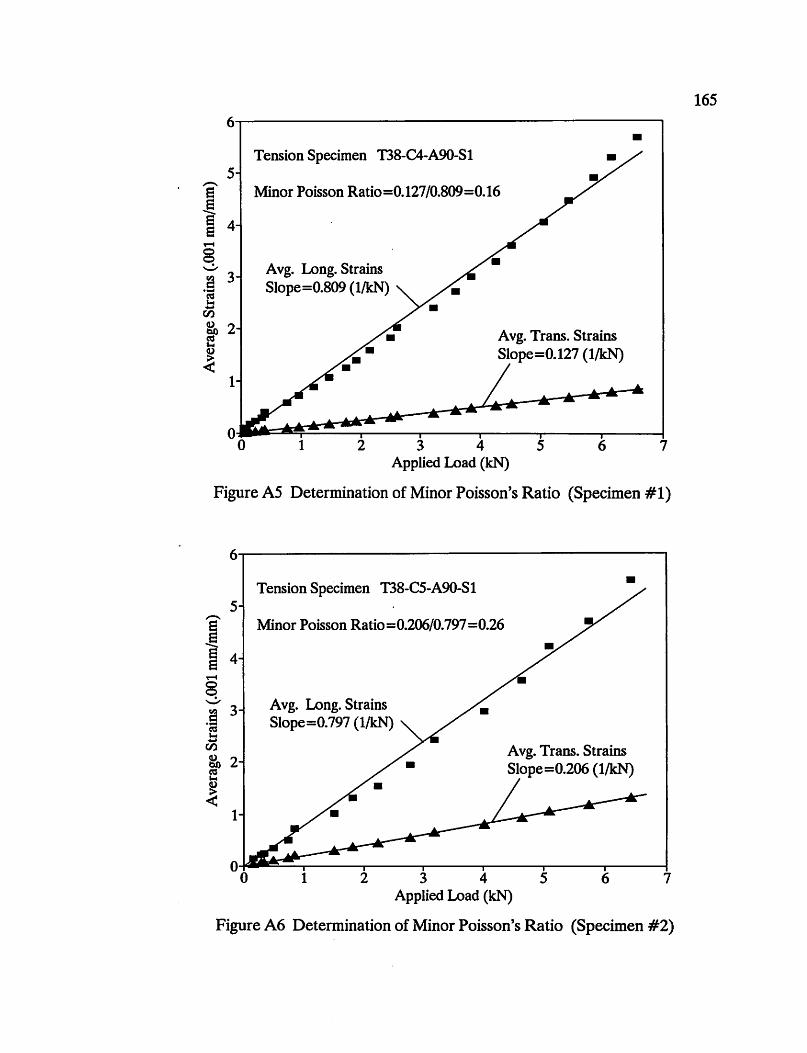
6~------------------------------------------'

Tension Specimen T38-C4-A90-S1

Minor Poisson Ratio =0. 127/0.809=0. 16



1 2 3 4 5 6 Applied Load (kN)

•

7

Figure AS Determination of Minor Poisson's Ratio (Specimen #1)

6~------------------------------------------.

5

1


Minor Poisson Ratio =0.206/0.797 =0.26


•


O~~~~--~~--~----~----~----~--~ o 123 456 7 Applied Load (kN)

Figure A6 Determination of Minor Poisson's Ratio (Specimen #2)

165

6~-----------------------------------------,

5

1


Minor Poisson Ratio =0.150/0.766=0.20

Avg. Long. Strains Slope = 0.766 (1/kN)


1 2 3 4 5 6 Applied Load (kN)

•

7

Figure A 7 Determination of Minor Poisson's Ratio (Specimen #3)

166

SINGLE-BOLTED CONNECTIONS FOR ORTHOTROPIC · PDF fileORTHOTROPIC FIBRE-REINFORCED COMPOSITE...

Documents

Transcript of SINGLE-BOLTED CONNECTIONS FOR ORTHOTROPIC · PDF fileORTHOTROPIC FIBRE-REINFORCED COMPOSITE...