Pablo A. Baier*Departamento de MecatrônicaInstituto Federal de EducaçãoCiência e Tecnologia do CearáRua Estevão Remígio 1145,Limoeiro do Norte, CE, Brazil

Jürgen A. Baier-SaipDepartamento de MatemáticaFísica y EstadísticaUniversidad Católica del MauleAv. San Miguel 3605,Casilla 617, Talca, Chile

Klaus SchillingLehrstuhl für Informatik VIIJulius-Maximilians-UniversitätWürzburgAm Hubland, 97074 Würzburg,Germany

Jauvane C. OliveiraDepartamento de ComputaçãoLaboratório Nacional deComputação CientíficaAv. Getúlio Vargas 333,Petrópolis, RJ, Brazil

Presence, Vol. 25, No. 2, Spring 2016, 108–128

doi:10.1162/PRES_a_00250

© 2016 by the Massachusetts Institute of Technology

Simulator for Minimally InvasiveVascular Interventions: Hardwareand Software

Abstract

In the present work, a simulation system is proposed that can be used as an edu-cational tool by physicians in training basic skills of minimally invasive vascularinterventions. In order to accomplish this objective, initially the physical model ofthe wire proposed by Konings has been improved. As a result, a simpler and morestable method was obtained to calculate the equilibrium configuration of the wire. Inaddition, a geometrical method is developed to perform relaxations. It is particularlyuseful when the wire is hindered in the physical method because of the boundaryconditions. Then a recipe is given to merge the physical and the geometrical meth-ods, resulting in efficient relaxations. Moreover, tests have shown that the shape ofthe virtual wire agrees with the experiment. The proposed algorithm allows real-timeexecutions, and furthermore, the hardware to assemble the simulator has a low cost.

1 Introduction

Over the last decades, minimally invasive surgery (MIS) has revolu-tionized many surgical procedures (Basdogan, De, Kim, Muniyandi, Kim, &Srinivasan, 2004). The treatment is delivered using image guidance, so thatskillful instrument navigation and a thorough understanding of the anatomyare critical to avoid complications. According to Fuchs (2002), “. . . two majordrawbacks have emerged with the introduction of MIS: firstly, the prolongedlearning curve for most surgeons, in comparison to the learning process inopen surgery; and secondly, increased costs due to investment in the equipmentrequired and the use of disposable instruments . . .” Since the development ofMIS has a lesser sense of touch compared to open surgery, surgeons must relymore on the feeling of net forces resulting from tool–tissue interactions and,eventually, longer training is needed.

The combination of traditional learning methods and technology enhancestrainee satisfaction and skill acquisition level (Engum, Jeffries, & Fisher, 2003;Tsang et al., 2008). The training methods include live observation of proce-dures, practicing on mechanical models, and hands-on training using humancadavers or live animals. In the past, hands-on training was considered the

*Correspondence to pablo.baier@ifce.edu.br.

108 PRESENCE: VOLUME 25, NUMBER 2

Baier et al. 109

best available method (Lunderquist et al., 1995; Mori,Hatano, Maruyama, & Atomi, 1998). However, it hasethical issues and it is also expensive, owing to the costsassociated with the use of animals in the process andbecause the instruments can be used only once (Coles,Meglan, & John, 2011).

Several training sessions can be performed with theaid of simulation techniques, providing certain levels ofproficiency to the physician. Based on these findings, theU.S. Food and Drug Administration (FDA) acceptedthe proposal that considers a virtual reality simulator(VRS) as an important component of a training pack-age for carotid stenting: “Trainees would learn catheterand wire-handling skills on a high-fidelity VRS until thetrainees achieved a level of proficiency in didactic andtechnical skills” (Gallagher & Cates, 2004).

Cardiac catheterization is a minimally invasive pro-cedure commonly used to diagnose and treat heartconditions (Balaji & Shah, 2011). During catheter-ization, small tubes (catheters) are inserted into thecirculatory system through the femoral artery and veinas the preferred access sites (Kasper, 2015). Using X-rayfluoroscopy, information is obtained about blood flowand pressures within the heart, and it is determined ifthere are obstructions within the blood vessels feedingthe heart muscle. For interventional procedures (e.g.,stenting and balloon angioplasty), a wire (WI) must beinserted through the catheter and maneuvered in thecoronaries. Achieving optimal outcomes requires opera-tor skills in guiding the WI, as well as selecting and usingthe surgical tools (Moscucci, 2014).

In general, vascular simulators such as Angio Mentorby Simbionox, VIST system by Mentince and CATHISby CATHi GmbH are expensive and complex. However,they offer advantages: no radiation is required, specificcases can be handled with multiple difficulty levels, andthere are no additional costs per training session. Pro-cedures start with a needle insertion into the vascularsystem, but current commercial simulators skip this stepin order to reduce complexity and cost. The guidewireand the catheter are then manipulated within the vas-cular anatomy to navigate to the position of interest.The simulation can be used as an initial training step todevelop skills before further proceeding with training in

animals or humans (Alderliesten, Konings, & Niessen,2004). Simulators are able to differentiate advancedoperators from novice operators, suggesting that it isa valid tool in the assessment of performances (Tsanget al., 2008). VRS are not exclusively used for train-ing purposes because they can be easily customized toprovide both medical programs and certification boardswith an objective tool for assessing physician skill andknowledge (Willaert, Aggarwal, Herzeele, Cheshire, &Vermassen, 2012).

In this work, a complete system for the simulation ofminimally invasive vascular intervention is described.The environment is composed of a hardware that cap-tures the movements of the guidewire and an algorithmthat simulates the motion inside arteries. Furthermore,the commands of the C-arm (an X-ray source and imageintensifier) are incorporated into the hardware.

The major contributions are as follows:

• In comparison with the paper of Konings, van deKraats, Alderliesten, and Niessen (2003):

– The WI model is more accurate, especially whenthe bending is large.

– The update equations are simpler and thenumerical calculations faster.

– The WI segment can be introduced at once (itis not necessary to make subdivisions).

• A geometrical method is introduced, which helpsto improve the speed when the WI is hindered byboundary conditions.

• A hardware device is described, which is simple todeploy and low cost. This can help to disseminatethe technique and make it widespread.

2 Related Research

This work is based on the developments of Kon-ings et al. (2003) in an analytical approximation tothe problem of the guidewire. The algorithm is highlygeneric and has good convergence properties. It is basedon quasi-static mechanics, which models the guidewirepropagation without specific knowledge about frictionforces. The motion is considered to be the result of aforced translation of the proximal guidewire body into

110 PRESENCE: VOLUME 25, NUMBER 2

the introducer sheath, effected by the physician. Thetranslation is a stepwise process which calculates how theguidewire reacts to an introduction of a small WI seg-ment, giving a new steady-state position. Alderliesten,Konings, and Niessen (2007) improved the model,incorporating the friction between the guidewire andthe vasculature.

The guidewire is similar to the model of the rope(knot) proposed by Brown, Latombe, and Montgomery(2004) and extended by Müller, Kim, and Chentanez(2012) to simulate hair and fur. They apply the ideabased on “Follow the Leader,” which is a purely geo-metrical technique where a chain of particles defines acurve representing a rope. Each particle moves towardsits predecessor to enforce their mutual distance to beconstant. The speed of the algorithm for computingthe global shape of the rope saves time that can be usedon the collision detection and on the managementmodules.

The Cosserat continuum theory of thin objects(shells, rods, and points) can be used to model theguidewire (Pai, 2002; Rubin, 2000). Cao and Tucker(2008) employed the Cosserat method to explore thenonplanar nonlinear dynamics of elastic rods. Later,Gao et al. (2015) described the dynamic behavior ofthe guidewire with the Lagrange equations of motionand applied the penalty method to maintain the con-straints. They proposed a simplified solving procedure tointegrate the resulting equations more easily.

Another method to model the deformation of aguidewire or a similar body is a representation basedon the 3D beam theory (Przemieniecki, 1985). Theelementary stiffness matrix relates angular and spatialpositions of each end of a beam element to the appliedforces and torques. Duriez, Cotin, Lenoir, and Neu-mann (2006) improved the accuracy and treat geometricnonlinearities, while maintaining real-time computation.They considered a Finite Element Modeling approachand developed a new mathematical representation com-bined with an incremental technique, that allows forhighly nonlinear behavior. In particular, a new methodis presented for correctly handling contact response incomplex situations where a large number of nodes aresubject to nonholonomic constraints.

Some simulators also include interactive fluid dynam-ics of blood flow, volumetric contrast agent propagation,and real-time collision detection and response (Coleset al., 2011). Current efforts are aimed towards integrat-ing performance assessment and user guidance (Willaertet al., 2012).

One of the most time-consuming tasks in the sim-ulation is the calculation of energy gradients in thePhysical Relaxation (PR). This problem has previouslybeen addressed (Baier, Srinivasan, Baier-Saip, Voelker,& Schilling, 2015). In particular, an efficient collision–detection algorithm was developed based on spacepartitioning. Furthermore, a continuous vector field(modulus and direction) was proposed, giving a realis-tic representation of the WI-surface interaction. On theother hand, Luboz, Blazewski, Gould, and Bello (2009)introduced a simplified deformable vascular model, butit is not smooth and contains surface irregularities whichaffect the collision response.

Besides the virtual model, the simulator must cap-ture the WI motion. The hardware can be built, forexample, using an optical encoder (Kodama et al.,2012) or a haptic device (Luboz et al., 2009). Forinstance, the Vascular Simulation Platform by Xitact isspecifically designed to coaxially track a catheter and aguidewire. However, these solutions are expensive tobuy or difficult to assemble.

Another promising surgery technique uses teleop-eration. This technique protects the physician fromX-ray radiation and solves the lack of experienced physi-cians in remote areas (Yu, Guo, Guo, & Shao, 2015).The slave manipulator detects the force of a catheterbeing inserted into the blood vessels. Then the mastermanipulator produces an equal damping force basedon magnetorheological fluids. Since VRS is similarto teleoperation, any progress made on one front cancontribute to the other one.

3 Methods

The model of Konings et al. (2003) considers theWI as a discrete set of joints at positions x0, . . . , xn , withx0 fixed. There are n segments and the i-th segment

Baier et al. 111

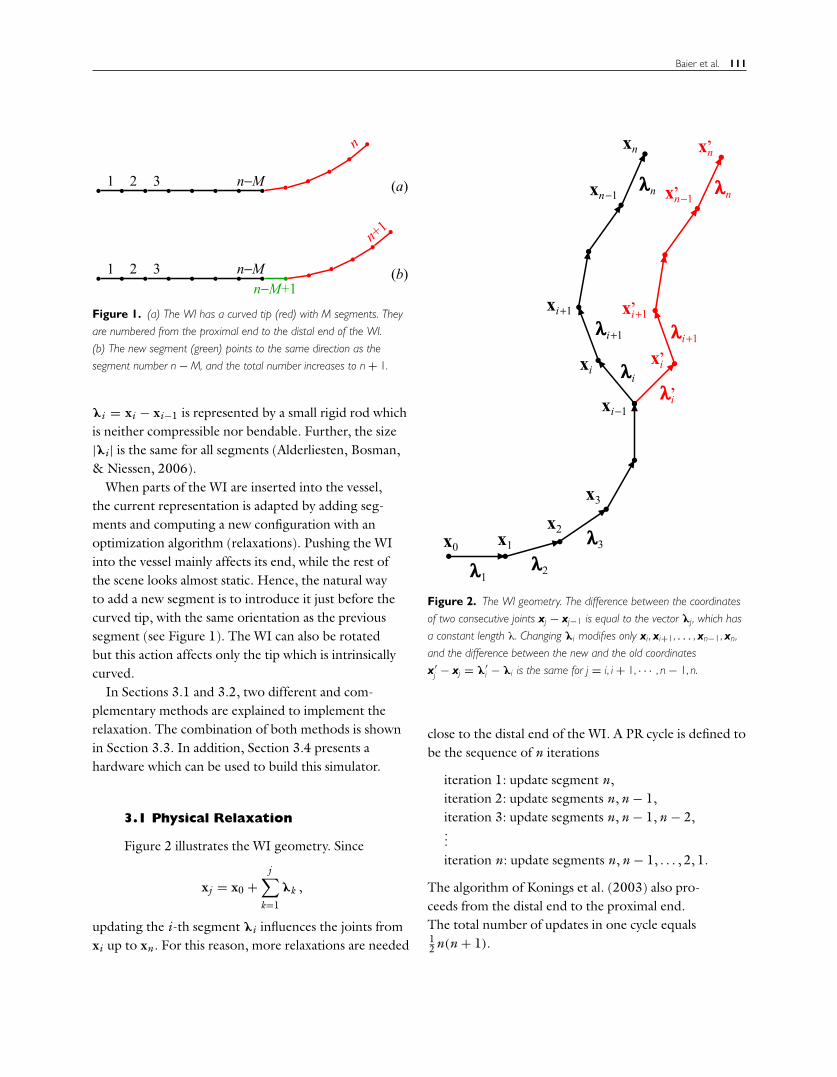
Figure 1. (a) The WI has a curved tip (red) with M segments. They

are numbered from the proximal end to the distal end of the WI.

(b) The new segment (green) points to the same direction as the

segment number n − M, and the total number increases to n + 1.

λi = xi − xi−1 is represented by a small rigid rod whichis neither compressible nor bendable. Further, the size|λi | is the same for all segments (Alderliesten, Bosman,& Niessen, 2006).

When parts of the WI are inserted into the vessel,the current representation is adapted by adding seg-ments and computing a new configuration with anoptimization algorithm (relaxations). Pushing the WIinto the vessel mainly affects its end, while the rest ofthe scene looks almost static. Hence, the natural wayto add a new segment is to introduce it just before thecurved tip, with the same orientation as the previoussegment (see Figure 1). The WI can also be rotatedbut this action affects only the tip which is intrinsicallycurved.

In Sections 3.1 and 3.2, two different and com-plementary methods are explained to implement therelaxation. The combination of both methods is shownin Section 3.3. In addition, Section 3.4 presents ahardware which can be used to build this simulator.

3.1 Physical Relaxation

Figure 2 illustrates the WI geometry. Since

xj = x0 +j∑

k=1

λk ,

updating the i-th segment λi influences the joints fromxi up to xn . For this reason, more relaxations are needed

Figure 2. The WI geometry. The difference between the coordinates

of two consecutive joints xj − xj−1 is equal to the vector λj , which has

a constant length λ. Changing λi modifies only xi , xi+1, . . . , xn−1, xn,

and the difference between the new and the old coordinates

x′j − xj = λ′

i − λi is the same for j = i, i + 1, · · · , n − 1, n.

close to the distal end of the WI. A PR cycle is defined tobe the sequence of n iterations

iteration 1: update segment n,iteration 2: update segments n, n − 1,iteration 3: update segments n, n − 1, n − 2,...iteration n: update segments n, n − 1, . . . , 2, 1.

The algorithm of Konings et al. (2003) also pro-ceeds from the distal end to the proximal end.The total number of updates in one cycle equals12 n(n + 1).

112 PRESENCE: VOLUME 25, NUMBER 2

To ensure numerical stability, every time an “action”is performed (add a segment, remove a segment, orrotate the WI) a Tip Relaxation is executed:

1. A number of 12 m(m + 1) updates (corresponding

to the first m iterations) is carried out. Thus, them segments closest to the tip are always updated.Since the actions take place just before the curvedtip (see Figure 1), m is chosen as M + 5 to ensurethat all affected segments will be updated at leastfive times before a new action is performed. How-ever, if the WI is very stiff, then it is necessary toreplace 5 by a bigger number.

2. Additionally, one update is executed for the seg-ment numbers n−m−5, n−m−10, n−m−15, . . .up to the proximal end of the WI. This ensuressome degree of relaxation besides the tip. Other-wise, if a large number of actions is performed in ashort time interval, the rest of the WI would be faraway from equilibrium.

The numerical performance can be increased ifincomplete cycles are carried out; that is, some ofthe last iterations (Alderliesten et al., 2007) are sup-pressed. In what follows, the physical model of theWI is improved and an updating recipe is given, whichis simpler to apply than the recipe of Konings et al.(2003).

3.1.1 Bending Energy. Consider the bendingenergy Ui of a WI segment (an arc) defined by threepoints xi−1, xi , and xi+1 (see Figure 3)

Ui = 12

EIi

R2i

si , (1)

where EIi represents the flexural rigidity, Ri is theradius, and si = Riθi is the arc length between xi−1 andxi (or equivalently between xi and xi+1). Note that Ui

does not represent the elastic energy between the pointsxi−1 and xi+1, but only half of this arc.

From Figure 3 it follows that the distance betweentwo points is given by λ = 2Ri sin(θi/2). HenceEquation 1 can be put in the form

Ui = EIi

2Riθi = EIi

λθi sin

θi

2. (2)

Figure 3. Three successive points xi−1 , xi , and xi+1 separated by an

equal distance λ = |λi| = |λi+1| define a circular arc of radius Ri and

angle 2θi .

For θi � 1 the last equation reduces to Equation 3 ofAlderliesten et al. (2004)

Ui = 12

EIi

λθ2

i .

The angle θi can be calculated using the formulacos θi = λi .λi+1/λ2. If the WI is intrinsically curved atjoint i, then λi+1 must be replaced by xi+1 − xi − ωi+1

(see Figure 4). Further, rotating the WI changes theorientation of ωi+1. Since

θ sinθ

2≈ (1 − cos θ) + 1

12(1 − cos θ)2 + 3

1280θ6 , (3)

up to fourth order in θi

Ui(λi , λi+1

) = EIi

12λ

[13 − 14 cos θi + cos2 θi

]

= Ci

12

[13 − 14

λi .λi+1

λ2 +(λi .λi+1

)2

λ4

],

(4)

where Ci = EIi/λ is a spring constant.

3.1.2 Energy Minimization. The orienta-tion of the i-th segment is updated (λi → λi + αi)while the others λj are kept constant, in such a waythat the energy decreases. The energy variation of

Baier et al. 113

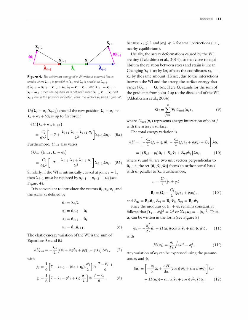
Figure 4. The minimum energy of a WI without external forces

results when λi−1 is parallel to λi , and λi is parallel to λi+1 .

If λi−1 = xi−1 − xi−2 + ωi , λi = xi − xi−1 , and λi+1 = xi+1 −xi − ωi+1 ; then the equilibrium is obtained when xi−2 , xi−1 , xi , and

xi+1 are in the positions indicated. Thus, the vectors ωi bend a free WI.

Ui(λi + αi , λi+1

)around the new position λi + αi →

λi + αi + δαi is up to first order

δUi(λi + αi , λi+1

)= Ci

6λ2

[− 7 + λi+1.λi + λi+1.αi

λ2

]λi+1.δαi . (5a)

Furthermore, Ui−1 also varies

δUi−1(λi−1, λi + αi

)= Ci

6λ2

[−7 + λi−1.λi + λi−1.αi

λ2

]λi−1.δαi . (5b)

Similarly, if the WI is intrinsically curved at joint i − 1,then λi−1 must be replaced by xi−1 − xi−2 + ωi (seeFigure 4).

It is convenient to introduce the vectors ui , ηi , εi , andthe scalar κi defined by

ui = λi/λ

ηi = ui−1 − ui

εi = ui+1 − ui

κi = ui .ui+1 . (6)

The elastic energy variation of the WI is the sum ofEquations 5a and 5b

δUelas = −Ci

λ

[(pi + qi)ui + piηi + qiεi

].δαi , (7)

with

pi = 16

[7 − κi−1 − (ui + ηi).

αi

λ

]≈ 7 − κi−1

6

qi = 16

[7 − κi − (ui + εi).

αi

λ

]≈ 7 − κi

6, (8)

because κi � 1 and |αi | � λ for small corrections (i.e.,nearby equilibrium).

Usually, the artery deformations caused by the WIare tiny (Takashima et al., 2014), so that close to equi-librium the relation between stress and strain is linear.Changing λi + αi by δαi affects the coordinates xi , · · · ,xn by the same amount. Hence, due to the interactionsbetween the WI and the artery, the surface energy alsovaries δUsurf = Gi .δαi . Here Gi stands for the sum ofthe gradients from joint i up to the distal end of the WI(Alderliesten et al., 2004)

Gi =n∑

j=i

∇j Usurf (xj ) , (9)

where Usurf (xj ) represents energy interaction of joint jwith the artery’s surface.

The total energy variation is

δU =[−Ci

λ(pi + qi)ui − Ci

λ(piηi + qiεi) + Gi

].δαi

= [(Bui − ρi)ui + Bvi vi + Bwiwi

].δαi , (10)

where vi and wi are two unit vectors perpendicular toui , i.e. the set {ui , vi , wi} forms an orthonormal basiswith ui parallel to λi . Furthermore,

ρi = Ci

λ(pi + qi)

Bi = Gi − Ci

λ(piηi + qiεi) , (10′)

and Bui = Bi .ui , Bvi = Bi .vi , Bwi = Bi .wi .Since the modulus of λi + αi remains constant, it

follows that |λi + αi |2 = λ2 or 2λi .αi = −|αi |2. Thus,αi can be written in the form (see Figure 5)

αi = − a2i

2λui + H (ai)(cos ψi vi + sin ψiwi) , (11)

with

H (ai) = ai

2λ

√4λ2 − a2

i . (11′)

Any variation of αi can be expressed using the parame-ters ai and ψi

δαi =[−ai

λui + dH

dai(cos ψi vi + sin ψiwi)

]δai

+ H (ai)(− sin ψi vi + cos ψiwi) δψi . (12)

114 PRESENCE: VOLUME 25, NUMBER 2

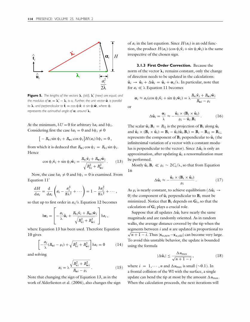
Figure 5. The lengths of the vectors λi (old), λ′i (new) are equal, and

the modulus of αi = λ′i − λi is ai . Further, the unit vector ui is parallel

to λi and perpendicular to ti = cos ψivi + sin ψiwi , where ψi

represents the azimuthal angle of αi around λi .

At the minimum, δU = 0 for arbitrary δai and δψi .Considering first the case δai = 0 and δψi �= 0[ − Bvi sin ψi + Bwi cos ψi

]H (ai) δψi = 0 ,

from which it is deduced that Bwi cos ψi = Bvi sin ψi .Hence

cos ψi vi + sin ψiwi = Bvi vi + Bwiwi√B2

vi + B2wi

. (13)

Now, the case δai �= 0 and δψi = 0 is examined. FromEquation 11′

dHdai

= ddai

(ai − a3

i8λ2 + · · ·

)= 1 − 3a2

i8λ2 + · · · ,

so that up to first order in ai/λ Equation 12 becomes

δαi =⎡⎢⎣−ai

λui + Bvi vi + Bwiwi√

B2vi + B2

wi

⎤⎥⎦ δai ,

where Equation 13 has been used. Therefore Equation10 gives[

−ai

λ(Bui − ρi) +

√B2

vi + B2wi

]δai = 0 (14)

and solving

ai = λ

√B2

vi + B2wi

Bui − ρi. (15)

Note that changing the sign of Equation 13, as in thework of Alderliesten et al. (2004), also changes the sign

of ai in the last equation. Since H (ai) is an odd func-tion, the product H (ai) (cos ψi vi + sin ψiwi) is the sameirrespective of the chosen sign.

3.1.3 First Order Correction. Because thenorm of the vector λi remains constant, only the changeof direction needs to be updated in the calculations:ui → ui + Δui = ui + αi/λ. In particular, note thatfor ai � λ Equation 11 becomes

αi ≈ ai(cos ψi vi + sin ψiwi) = λBvi vi + Bwiwi

Bui − ρi

or

Δui = αi

λ≈ − ui × (Bi × ui)

ρi − ui .Bi. (16)

The scalar ui .Bi = Bi‖ is the projection of Bi along ui

and ui × (Bi × ui) = Bi − ui(ui .Bi) = Bi − Bi‖ = Bi⊥represents the component of Bi perpendicular to ui (theinfinitesimal variation of a vector with a constant modu-lus is perpendicular to the vector). Since Δui is only anapproximation, after updating ui a renormalization mustbe performed.

Mostly ui .Bi � ρi ∼ 2Ci/λ, so that from Equation16

Δui ≈ − ui × (Bi × ui)

ρi. (17)

As ρi is nearly constant, to achieve equilibrium (Δui →0) the component of ui perpendicular to Bi must beminimized. Notice that Bi depends on Gi , so that thecalculation of Gi plays a crucial role.

Suppose that all updates Δui have nearly the samemagnitude and are randomly oriented. As in randomwalks, the average distance covered by the tip when thesegments between i and n are updated is proportional to√

n + 1 − i. Thus |xn,new−xn,old| can become very large.To avoid this unstable behavior, the update is boundedusing the formula

|Δui | ≤ Δumax√n + 1 − i

, (18)

where i = 1, · · · , n and Δumax is small (∼0.1). Ina frontal collision of the WI with the surface, a singleupdate can bend the tip at most by the amount Δumax.When the calculation proceeds, the next iterations will

Baier et al. 115

bend the tip further until |Δui | naturally decreases andthe WI approaches equilibrium.

The updates Δui for small i are tiny because they arebounded by Equation 18. Hence, instabilities are dissi-pated and do not propagate to the proximal end of theWI. It is the tip of the WI (i close to n) which plays animportant role in the simulation and, in this region, ahigher number of updates is performed. Since the relax-ation is stable, there is no need to introduce the segmentin small steps as in the work of Alderliesten et al. (2004),and it can be performed at once.

If |Bi | � ρi , the update will be small. In this case, thedenominator in Equation 16 is positive and the updatemoves the WI in a direction so as to cancel Bi . But in afrontal collision of the tip with the artery, Bi can becomevery large because of Gi . If the sign of the denominatoris negative, Bi will increase instead of canceling, and thecalculations diverge. In particular, for ρi − ui .Bi ≈ 0the modulus |αi | becomes larger than 2λ, which is geo-metrically impossible. In such cases, the approximationdH /dai = 1 fails.

To overcome this drawback, Equation 14 should beconsidered without approximations

−ai

λ(Bui − ρi) + 2λ2 − a2

i

λ

√4λ2 − a2

i

√B2

vi + B2wi = 0,

and solve numerically for ai . However, a simple estima-tion for Δui can be found. Taking the absolute value inthe denominator of Equation 16

Δui = − ui × (Bi × ui)

|ρi − ui .Bi | , (19)

the update will always be in the right direction. Notethat using Equation 17 in place of Equation 19 givessimilar results. The magnitude of the correction can stillbe large, but since |Δui | is bounded and ui is renormal-ized after each update, it poses no problem. ApplyingEquations 18 and 19 in the Tip Relaxation results in astable algorithm, even if in a short time interval, a largenumber of actions are performed by the user.

Lastly, it is observed that Equation 19 basicallyinvolves the calculation of Bi and the computationof scalar and cross products with ui . On the otherhand, Equation 11 of Alderliesten et al. (2004) works

implicitly with an orthonormal basis. It is necessary tocalculate the projections of Bi in this base, to determinethe modulus ai , the angle ψi , and then to constructthe vector αi again using the base. Thus, the methoddeveloped in this work is simpler to apply.

3.1.4 Pseudocode.

void PhysicalUpdate(segment i){1. calculate the gradient Gi , see Equation 9;2. calculate the update Δui , see Equations 18and 19;3. update ui and renormalize;4. update xi , xi+1, · · · , xn ;5. update ωi , ωi+1, · · · , ωn ;

}

The function PhysicalUpdate implements themethod described in this section. Next, the process-ing time (PT) spent in calling the function during acomplete PR cycle is analyzed.

For a segment number i, the calculation of Gi

involves the collision test for n − i segments. Duringthe cycle of the PR, this function is called 1

2 n(n + 1)

times, and the total number of collision tests in one cycleis 1

6 n(n + 1)(n + 2). If there is a collision for j > i, then∇j Usurf (xj ) must be calculated. The number of timesthe gradient is computed depends on j . For example, ifj = n/2 the computation is repeated 1

8 n(n + 2) ≈ n2/8times, and in general it will be a fraction of n2. Thus, thePT of line 1 has the form 1

6 n(n + 1)(n + 2)T1 + n2T2,where T1 and T2 are positive constants.

The lines 2 and 3 involve a single execution, so thatthe PT of one cycle is proportional to 1

2 n(n + 1).Finally, lines 4 and 5 give a contribution similar to thenumber of collision tests executed, i.e. proportionalto 1

6 n(n + 1)(n + 2). Hence, the estimated PT of thephysical update cycle is

tphy = tp1n + tp2n2 + tp3n3

≈ tp2n2 + tp3n3 . (20)

In the last line, the PT is approximated by the two maincontributions for large n.

116 PRESENCE: VOLUME 25, NUMBER 2

Since Tip Relaxation plays a central role in the algo-rithm, its PT will also be examined. In the first part,when the first m segments are updated, the PT is similarto Equation 20 but with n → m = M + 5 (a con-stant). In the second part, when the segment numbersn − m − 5, n − m − 10, n − m − 15, · · · are updatedonce, instead of 1

2 n(n + 1) only ∼ (n − m)/5 stepsare executed. Hence, for large n the term n2/2 must bereplaced by n/5 in Equation 20. The overall result is

ttip ≈ tp1m + tp2m2 + tp3m3 + tp3

(2n5

)3/2

= const + tp4n3/2 . (21)

For example, if m = 5 + 5 and n = 250, then m3 =1000 = (2n/5)3/2, that is, the constant has the sameorder of magnitude as the last term in Equation 21.

3.2 Geometrical Relaxation

Consider the problem of finding the minimumenergy of a homogeneous WI (EI = const) with the fol-lowing boundary conditions. The end points xμ and xν

are fixed as well as the tangent vectors to the trajectoryxμ and xν (the dot denotes differentiation with respectto the curve parameter τ). Between these points there isno contact with the surface and the total length of thecurve is not fixed.

3.2.1 Bending Energy. Here, it is necessary toderive a generalization of Equation 2 when the modu-lus λi = |λi | is variable. In Figure 6 the three pointsxi−1, xi , and xi+1 are joined by two arcs having thesame angle θi but different radii Ri and Ri+1. It is alsopossible to join the points using the same radius and dif-ferent angles, but the calculations become cumbersome.The sum of the energies in half arc under and in half arcabove the point xi is

Ui = 12

EIR2

i

si2

+ 12

EIR2

i+1

si+1

2

= EI2

(θi

2Ri+ θi

2Ri+1

)

= EI2

(1λi

+ 1λi+1

)θi sin

θi

2,

Figure 6. Three points xi−1 , xi , and xi+1 are separated by different

distances |λi| �= |λi+1|. The two circular arcs have the same angle θi

but the radii Ri and Ri+1 are not equal.

because sin(θi/2) = λi/2Ri = λi+1/2Ri+1. UsingEquation 3 with cos θi = ui .ui+1 results in

Ui = EI12

(1λi

+ 1λi+1

)13 − 14 ui .ui+1 + (ui .ui+1)2

2.

3.2.2 Energy Minimization. Since only λi andλi+1 are functions of xi , it follows that Ui−1, Ui , andUi+1 depend on this coordinate. Omitting the con-stant multiplicative factor EI /12, it suffices to analyzethe function

Ψ(xi) =(

1λi−1

+ 1λi

) 13 − 14 κi−1 + κ2i−1

2

+(

1λi

+ 1λi+1

)13 − 14 κi + κ2

i2

+(

1λi+1

+ 1λi+2

) 13 − 14 κi+1 + κ2i+1

2. (22)

Notice that Ψ does not contain any physical parameterand depends solely on the geometry.

The label ∗ will be used to refer to the coordinates ofthe improved curve. In order to minimize Ψ, substitutex∗

i by x∗i + yi yi + zi zi , where yi and zi are orthogonal to

the vector xi+1 − xi−1. The calculation of yi and zi canbe carried out using the Hessian matrix and the gradient(

Ψyy ,i Ψyz,i

Ψyz,i Ψzz,i

) (yi

zi

)= −

(yi .∇iΨ

zi .∇iΨ

). (23)

Baier et al. 117

The Hessian matrix gives essentially a metric to findthe length of the update

∣∣x∗i,new − x∗

i,old

∣∣ in the direc-tion of steepest descent. This direction is determined bythe negative components of the gradient in the planedefined by yi and zi . Near the minimum, the Hessianapproaches a constant. Thus, the matrix elements can becomputed numerically

Ψyy ,i = 1(δλ)2

[Ψ(x∗

i + δλyi) − 2Ψ(x∗i ) + Ψ(x∗

i − δλ yi)]

Ψyz,i = 14(δλ)2

[Ψ(x∗

i + δλ yi + δλ zi)

− Ψ(x∗i + δλ yi − δλ zi)

− Ψ(x∗i − δλ yi + δλ zi)

+ Ψ(x∗i − δλ yi − δλ zi)

]Ψzz,i = 1

(δλ)2

[Ψ(x∗

i + δλzi) − 2Ψ(x∗i ) + Ψ(x∗

i − δλ zi)],

(23a)

where δλ = λ/104 for calculations performed withdouble precision.

On the other hand, the gradient is very sensitive tonumerical round off errors near the minimum. Hence∇iΨ must be determined analytically with the help of∇iλ

∗i−1 = 0, ∇iλ

∗i = u∗

i , ∇iλ∗i+1 = −u∗

i+1, ∇iλ∗i+2 = 0,

and

∇iκ∗i−1 = u∗

i−1 − κ∗i−1u∗

i

λ∗i

∇iκ∗i = u∗

i+1 − κ∗i u∗

i

λ∗i

− u∗i − κ∗

i u∗i+1

λ∗i+1

∇iκ∗i+1 = − u∗

i+2 − κ∗i+1u∗

i+1

λ∗i+1

. (23b)

The minimization update is executed for the sequencei = μ + 1, μ + 2, · · · , ν − 1, which is defined to be aniteration in the geometrical relaxation (GR) cycle. Afterrepeating ∼ ν − μ times the iteration, the modulus of∇iΨ is reduced by a considerable amount, i.e. the curveapproaches the desired solution. Hence, one Geomet-rical Relaxation (GR) cycle consists of ν − μ iterations,which has (ν − μ)(ν − μ − 1) ≈ (ν − μ)2 minimizationupdates.

Observe that the vectors yi and zi are calculated onlyat the beginning of the minimization procedure. Since

Figure 7. (a) Original curve xi (red), curve after executing the

energy minimization x∗i (green), and displaced points x′

i (black).

(b) Closer view of three coordinates x∗i−2 , x∗

i−1 , and x∗i after the

minimization. The unit vector u∗i points from x∗

i−1 to x∗i , and the vector

bij goes from x′j−1 to the line passing through x∗

i−1 and x∗i .

The distance between x′j−1 and x′

j equals λ.

the plane over which the point x∗i can move is kept con-

stant, the possibility λ∗i → 0 is ruled out and numerical

instabilities are avoided.

3.2.3 Point Slide. After executing the energyminimization, the point must be shifted (x∗

i → x′i) to

restore |λ′i | = λ. Specifically, x′

i is displaced followingthe polyline to obtain |x′

i − x′i−1| = λ as depicted in

Figure 7(a), an idea which is based on the “Follow theLeader” technique.

To find x′j explicitly, consider Figure 7(b). Let x∗

i−1and x∗

i be two vertices in the polyline such that |x∗i−1 −

x′j−1| < λ and |x∗

i − x′j−1| > λ. Then construct the

vector

bij = u∗i × [

(x∗i−1 − x′

j−1) × u∗i]

. (24)

The j -th coordinate is calculated with the formula

x′j = x′

j−1 + bij + u∗i

√λ2 − |bij |2 . (25)

In particular, at the beginning x′μ = xμ.

The previous displacement is performed using a linearinterpolation between x∗

i−1 and x∗i . It is not difficult to

find a second order correction for the interpolated pointx′

j . This procedure is illustrated in Figure 8: the point x′j

is displaced in the direction of the unit vector e∗i which is

perpendicular to x∗i −x∗

i−1 = λ∗i = λ∗

i u∗i . In order to find

118 PRESENCE: VOLUME 25, NUMBER 2

Figure 8. Second order correction εije∗i to the coordinate x′

j . The

displacement is indicated by the green arrow. The arc segment has an

angle θ∗i and a radius R∗

i . The distance between x∗i−1 and x∗

i is λ∗i ,

and the distance between x′j and x∗

i is dij .

a formula for e∗i , let v∗

i− and v∗i+ be two vectors parallel

to u∗i−1×u∗

i and u∗i ×u∗

i+1 respectively. Then e∗i is chosen

to point in the direction u∗i × (v∗

i− + v∗i+). Notice that e∗

ilies in the average of the planes specified by u∗

i−1, u∗i and

by u∗i , u∗

i+1. But if v∗i−.v∗

i+ ≤ 0 it is not convenient toperform the second order correction, because the curvehas an inflection and the circumference in Figure 8 is nolonger a good approximation.

To determine the length εij of the displacement, firstcalculate the radius of the circumference

R∗i = λ∗

i

2 sin(θ∗i /2

) = λ∗i√

2 − 2 cos θ∗i

.

The cosine of the angle θ∗i can be found with the dot

product u∗i−1.u∗

i or u∗i .u∗

i+1. In general, these prod-ucts will be different and cos θ

∗i is set equal to the mean

value. Then the radius becomes

R∗i = λ∗

i√2 − u∗

i .(u∗

i−1 + u∗i+1

) . (26)

Let dij be the distance between xi and x′j . From Figure 8

it is inferred that

εij =√

(R∗i )2 −

(λ∗

i2

− dij

)2

−√

(R∗i )2 −

(λ∗

i2

)2

.

(27)

Finally, the replacement x′j → x′

j + εij e∗i is carried out.

Observe that, after replacing, the modulus of the vectorλ′

j = x′j − x′

j−1 becomes slightly different from λ. There-fore, it is necessary to move the point x′

j to fix the lengthof λ′

j .The second order correction is in practice very small.

But it is important for points close to the surface becauseit avoids abrupt changes of the interaction force in thePR.

3.2.4 Cubic Spline. To select the interval toapply the GR, it is desirable to have an approximate ana-lytical solution x(τ) with boundary conditions xμ, xμ,xν, and xν. The two-dimensional static Euler–Bernoulliequation describing a beam having a small deflection υ is

d4υ

dτ4 = QEI

.

For zero transverse load (Q = 0) the solution is a cubicspline. The four integration constants are determinedusing the boundary conditions υ(τμ), υ(τμ), υ(τν), andυ(τν).

In 3D the cubic spline becomes

xcub = (1 − τ)xμ + τxν + τ(1 − τ)[(1 − τ)sμ − τsν

],

(28)

where τ ∈ [0, 1]. Let Xμν = xν − xμ and Uμ, Uν be twounit vectors parallel to xμ, xν respectively. If the vectorssμ and sν (associated with the cubic dependencies on τ)are perpendicular to the line (1 − τ)xμ + τxν connectingthe points xμ and xν, then

sμ = |Xμν|2Xμν.Uμ

Uμ − Xμν

sν = |Xμν|2Xμν.Uν

Uν − Xμν . (29)

Baier et al. 119

A small deflection occurs when Uμ and Uν are nearlyparallel to Xμν = Xμν/|Xμν|.

3.2.5 Interval Selection. To find a suitable inter-val to apply the GR, the first step is to search for intervalswhose end points xμ, xν are close to the surface, andwhose inner points xμ+1, · · · , xν−1 are far from the sur-face. Specifically, a point is considered to be close (far)when the distance to the surface is smaller (larger) than5% of the average artery diameter. It will be seen that inthe PR cycle a point near to the surface can be bouncing(Section 4.4).

Next, discard intervals having few segments, say lessthan 5. Also exclude the tip of the WI, which is curved,and any other interval having a nonconstant flexuralrigidity.

For each of the remaining intervals execute the fol-lowing operations. Given xμ and xν with tangent vectorsxμ = uμ+uμ+1 and xν = uν+uν+1, determine the cubicspline xcub,i . Then calculate the mean square deviation

σ2μν = 1

ν − μ

ν∑i=μ

σ2i , (30)

where σ2i = |xi − xcub,i |2. The cases of interest occur

when the deviation σμν is large. Moreover, the cubicspline is not a good approximation unless Uμ and Uν

are nearly parallel to Xμν; that is, a bad approximationresults if 1 + Uμ.Xμν or 1 + Uν.Xμν are small. Hence,calculate the following figure of merit

χμν = (1 + Uμ.Xμν)2(1 + Uν.Xμν)

2 σμν, (31)

and select the interval with the largest χμν.It is not mandatory to move the points when the dis-

tance between xi and xcub,i is small, so that a reducedinterval can be chosen. If σi < 0.10 σμν for i =μ + 1, μ + 2, · · · , μ+, then replace μ → μ+. Like-wise, if σi < 0.10 σμν for i = ν − 1, ν − 2, · · · , ν−,then replace ν → ν−. Note that a shorter intervaldecreases the PT to calculate the improved curve, whichis proportional to (ν − μ)2. Moreover, the angles�(Nμ, Uμ), �(Nν, Uν) are likely bigger than the angles�(Nμ+, Uμ+), �(Nν−, Uν−), where Ni stands for avector normal to the artery’s surface. Hence, there is a

smaller probability that the improved curve interceptsthe surface when the interval is reduced.

If an interception occurs, then do not update xi → x∗i

but use a linear interpolation xi → ζx∗i + (1 − ζ)xi with

ζ ∈ (0, 1). In practice, ζ should be large but it must avoidthe intersection. Further, to ensure numerical stability itis convenient to limit ζ such that the tip of the WI doesnot displace a distance greater than λ. Thus, after exe-cuting the GR check if |xn − x′

n| < λ, otherwise decreaseζ and repeat the interpolation.

3.2.6 Pseudocode.

void GeometricalRelaxation(void){6. select the interval μ < i < ν to apply the GR, seeSection 3.2.5;7. execute ν − μ iterations (with a total of (ν − μ)2

energy minimization updates), see Section 3.2.2;8. shift the points xμ+1, xμ+2, · · · , xn to restore thelength |λj | = λ, see Section 3.2.3;

}

Now, the PT of the GR will be analyzed. The num-ber of operations necessary to determine the interval inline 6 is proportional to n. Let us change the resolutionof the WI in such a way that λ ∝ 1/n. If the shape ofthe WI does not vary appreciably, then the position ofthe points xμ1, xν1 before and xμ2, xν2 after changingthe resolution will be nearly the same. Thus, it is con-cluded that μ, ν are proportional to n and the PT in line7 scales with n2 (see Section 3.2.5). Similarly, the PT inline 8 (proportional to n −μ) scales with n. In summary,the average PT of the GR cycle is

tgeo = tg1n + tg2n2 . (32)

3.3 Combination of PR and GR

A major drawback of the PR is that the WImoves as rigid structure about a fixed point. Depend-ing on the boundary conditions this can be veryhard to achieve. For example, the segment P1P2 inFigure 9 needs to turn up but it is hindered by contactpoints.

120 PRESENCE: VOLUME 25, NUMBER 2

Figure 9. WI segments inside an artery. In order to relax, the

segment P1P2 should rotate upwards about point P1 as indicated by

the arrow. Note that from P2 to P6 the WI is rigid, so that the resulting

translation is hindered by the contact points P3 and P4 . Nor can it

move downwards because of P5 . The GR is not subjected to this

restriction, since from P3 up to P6 the WI can slide. It is especially

designed to relax intervals like from P0 to P3 (red).

One possible solution is the GR developed in Section3.2, which allows the WI to slide. The GR is executedafter a PR cycle (see Figure 10) and does not inter-fere with it, because the GR is much faster than the PR(Section 4.3). In particular, if a user action takes placeduring a PR or a GR cycle, then it is interrupted anda Tip Relaxation is executed (this ensures stability).Moreover, the shape of the tip (where the actions takeplace) looks more natural. The combination of bothtechniques results in a more realistic WI behavior thanusing only the relaxation proposed by Konings et al.(2003).

3.4 Wire Device

Here, a simple device to capture the WI motion isdescribed (see Figure 11). In cardiovascular procedures,the WI sweeps at most a length of 150 mm inside thecoronary. In view of this fact, the required materials areas follows:

• Support box.• Pipe tube of length 320 mm, with a small window in

the middle.• Light and opaque cylinder 170 mm long.

Figure 10. Workflow. In the “Tip Relaxation” (Section 3.1) the

function PhysicalUpdate is applied to the tip of the WI and also

to some selected segments. When the “Physical Relaxation” is called,12 m(m + 1) updates are executed. The PR is completed if the cycle

ends; that is, after 12 n(n + 1) updates. In the same way, when the

“Geometrical Relaxation” is called, m(m + 1)/(ν − μ) iterations are

executed to improve the curve. The GR is completed after ν − μ

iterations.

• Optical mouse with a precision of 1200 dpi orhigher.

• Set of catheter and steerable guidewire with 150mm free length.

The WI is attached to the cylinder, which is put insidethe pipe. In particular, the friction between the pipe andthe cylinder must be small. The mouse is fixed over thepipe in such a way that the light-emitting diode stayson the window. Moreover, it is possible to add extracommands to improve the simulator. For instance, themouse buttons can simulate the contrast injection orthe activation of the X-ray employed in video genera-tion. Also, a USB-joystick with two axes can be used tochange the C-arm perspective.

Baier et al. 121

Figure 11. Photography (top-view) and sketch (cross-view) of the

WI device. The pipe has a small window and the mouse is over the

window. Translating and rotating the WI also translates and rotates the

cylinder, which is captured by the mouse.

The WI movement is transferred to the cylinder andcaptured by the mouse according to:

• Pushing and pulling the WI = cursor up and down.• Rotating the WI = cursor left and right.

The mouse must be aligned with the axis of the cylinder;otherwise translations and rotations will appear mixed.Depending on the mouse resolution, pointer speed,and cylinder diameter, different cursor movements areobtained. Hence, a calibration is required to providea correct feedback to the user. As an alternative to theoptical mouse, a piezoelectric captor can be connectedto detect the cylinder motion.

The device has the technology of an optical mouse,whose movements can be read with basic functions inany programming language. The manufacturing costis low and the portability allows the device to be usedwithout platform restrictions.

Since the tip of the WI is soft, the contribution tothe sense of touch is not significant. The force feed-back is due mainly to the friction between the WI andthe catheter (Takashima et al., 2014). In our device thisforce is already embodied because the WI slides insidethe catheter. This removes the complex problem of cou-pling haptics and graphic simulation, especially becausethey proceed at different frequencies (of the order of1000 Hz and 30 Hz, respectively).

4 Technical Evaluation

In order to validate the usefulness and to examinethe limitations of the methods developed in this work,several analyses are performed including the stability, WIresolution, and PT of the PR and GR. Moreover, theinteraction between the WI and the artery is inspected.Finally, the present model is compared with the modelof Alderliesten et al. (2004).

In the simulations, a flexural rigidity EI equal to6.35 × 10−9 Nm2 is assumed. The algorithm wasimplemented in C++, and the tests were performed ina computer having a Intel Core i7-4500U (2.40 GHz)and 16 GB of RAM.

4.1 Stability Analysis

The total PT was tested for the artery shown inFigure 12, which includes a T-like and a Y-like bifur-cation (Baier et al., 2015). In the first part of thesimulation, the WI is outside the artery and it is quicklypushed inside (only the Tip Relaxation is applied). Theresult (green curve) looks unphysical, but the algorithmdoes not crash during a fast insertion of the WI. The sta-bility is also verified if λ increases to 2.5 mm, so that adeeper frontal collision occurs at the T-like bifurcation.However, if the WI becomes very stiff (a huge flexu-ral rigidity), then it will “perforate” the artery (like aneedle) and the behavior becomes unstable.

In contrast, the algorithm of Alderliesten et al. (2004)demands a slow insertion of the WI; otherwise it cancrash. For example, in numerical tests Konings et al.(2003) and Alderliesten et al. (2007) used an internal

122 PRESENCE: VOLUME 25, NUMBER 2

Figure 12. Artery with a T-like and a Y-like bifurcation. (Left) The WI has 250 segments, λ = 1 mm, and it has been quickly inserted into the

artery (green curve). In this part, the program executed only Tip Relaxations and the time consumed was 0.24 seconds. In the second part, no

action takes place and a combination of 100 relaxation cycles (Physical and Geometrical) is executed, so that equilibrium is attained (blue curve).

The coordinates indicate the location of some WI joints. (Right) Mockup representing the stiff artery. The WI inserted in the artery has the same

shape as the blue curve. The average separation between the physical WI and the blue curve is 0.262 mm with a standard deviation of 0.227

mm. Hence, the calculations with the model developed in this work give a realistic result.

stepsize smaller than λ/10. Since they insert the newsegment in the proximal end of the WI, to guaranteestability they must execute at least ten times the com-plete relaxation cycle before a new action takes place.As in Equation 20, their PT is proportional to n3 forlarge n, but in our case it is proportional to a constantplus n3/2 (see Equation 21). Hence, this method worksmuch faster under stress conditions.

In the second part of the simulation, a large numberof cycles are executed. The result is the blue curve inFigure 12 (left) and a numerical comparison with exper-iment (right) shows that the calculations are truthful.Besides the specific case in Figure 12, several paths havebeen tested and the results were always good.

In real procedures, the physician should not insertthe WI quickly, to avoid vascular damage. For securityreasons, in the specific case of teleoperation the speedof the slide platform is less than 10 mm/s (Yu et al.,2015). On the other hand, one of the most annoyingsituations encountered by users in simulators is the time

delay between the action and the response. In our sim-ulator (green curve in Figure 12) the average speed was(250 mm)/(0.24 s) ≈ 1 m/s.

4.2 Segment Size

The PT will depend on the artery’s resolutionand on the size of the segment λ. The method of Baieret al. (2015) to calculate Gi is almost independent ofthe artery’s resolution. This artery model refers to ageometry which does not depend on time. Otherwisethe proposed method is not feasible because changesof shape make it more difficult to use precomputeddata structures for expediting collision tests duringsimulation (Brown et al., 2004).

If λ decreases but the WI length remains the same,the total number of segments n increases. Hence,with a higher WI resolution the PT becomes longer.To determine the optimal segment size (Alderliestenet al., 2004), the influence of λ on the shape of the

Baier et al. 123

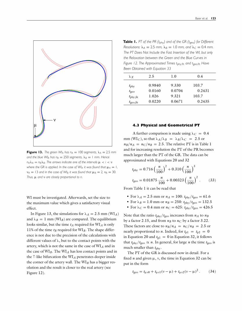
Figure 13. The green WIA has nA = 100 segments, λA = 2.5 mm

and the blue WIB has nB = 250 segments, λB = 1 mm. Hence

nAλA = nBλB. The arrows indicate one of the intervals μ < i < ν

where the GR is applied. In the case of WIA it was found that μA = 1,

νA = 13 and in the case of WIB it was found that μB = 2, νB = 30.

Thus, μ and ν are closely proportional to n.

WI must be investigated. Afterwards, set the size tothe maximum value which gives a satisfactory visualeffect.

In Figure 13, the simulations for λA = 2.5 mm (WIA)and λB = 1 mm (WIB) are compared. The equilibriumlooks similar, but the time tA required for WIA is only11% of the time tB required for WIB . The shape differ-ence is not due to the precision of the calculations withdifferent values of λ, but to the contact points with theartery, which is not the same in the case of WIA and inthe case of WIB . The WIA has less contact points and inthe T-like bifurcation the WIA penetrates deeper insidethe corner of the artery wall. The WIB has a bigger res-olution and the result is closer to the real artery (seeFigure 12).

Table 1. PT of the PR (tphy) and of the GR (tgeo) for DifferentResolutions: λA = 2.5 mm, λB = 1.0 mm, and λC = 0.4 mm.The PT Does Not Include the Fast Insertion of the WI, but onlythe Relaxation between the Green and the Blue Curves inFigure 12. The Approximated Times tphy,fit and tgeo,fit HaveBeen Obtained with Equation 33

λX 2.5 1.0 0.4

tphy 0.9840 9.330 103.7tgeo 0.0160 0.0704 0.2431tphy,fit 1.026 9.321 103.7tgeo,fit 0.0220 0.0671 0.2435

4.3 Physical and Geometrical PT

A further comparison is made using λC = 0.4mm (WIC ), so that λA/λB = λB/λC = 2.5 ornB/nA = nC/nB = 2.5. The relative PT is in Table 1and for increasing resolution the PT of the PR becomesmuch larger than the PT of the GR. The data can beapproximated with Equations 20 and 32

tphy = 0.716( n

100

)2 + 0.310( n

100

)3

tgeo = 0.01875n

100+ 0.00323

( n100

)2. (33)

From Table 1 it can be read that

• For λA = 2.5 mm or nA = 100: tphy/tgeo = 61.6• For λB = 1.0 mm or nB = 250: tphy/tgeo = 132.5• For λC = 0.4 mm or nC = 625: tphy/tgeo = 426.5

Note that the ratio tphy/tgeo increases from nA to nB

by a factor 2.15, and from nB to nC by a factor 3.22.These factors are close to nB/nA = nC/nB = 2.5 ornearly proportional to n. Indeed, for tp1 = tp2 = 0in Equation 20 and tg1 = 0 in Equation 32, it followsthat tphy/tgeo ∝ n. In general, for large n the time tgeo ismuch smaller than tphy.

The PT of the GR is discussed now in detail. For afixed n and given μ, ν, the time in Equation 32 can beput in the form

tgeo = tμν0 + tμν1(ν − μ) + tμν2(ν − μ)2 . (34)

124 PRESENCE: VOLUME 25, NUMBER 2

Figure 14. GR relaxation time tgeo as function of the interval length

ν − μ. The blue color represents the WIB with nB = 250 segments

(blue curve in Figure 13) and the red color represents the WIC with

nC = 625 segments (not shown in Figure 13). The points are the PT

measured in numerical simulations and the lines are the fits performed

with Equation 34.

The results for WIB and WIC are shown in Figure 14.Note that there are points missing in the numericalexperiments because in the calculations not every inter-val size ν − μ occurs. In particular, the blue points arenot far from the red points for ν − μ ≈ 60.

The blue points in the interval 20 < ν − μ < 30correspond to the red points in the interval 60 < ν −μ < 90, because μ and ν are nearly proportional to n(Section 3.2.6). Also, the blue points in 55 < ν−μ < 60correspond to the red points in 165 < ν − μ < 175.

The PT for a single energy minimization does notdepend on the total number of WI segments. Since(ν − μ)2 minimization updates are executed in a GRcycle, the quadratic coefficient in Equation 34 shouldalways be the same. Indeed, this coefficient is equal totg2 = 0.003663, 0.003586 for WIB , WIC , respectively,and the difference is 2%.

It is also interesting to compare the PT using the PR(case P ) and using both the PR and the GR (case G).The outcomes are highly dependent on the initial WI

Figure 15. Initial curve (green) and the final equilibrium curve (blue)

obtained after a very long relaxation time. The final result is the same

with or without the GR. The analysis is focussed in the WI portion

located inside the gray box, which goes from WI segment number 90

to 95. In this interval are seen the most relevant changes during

relaxation.

shape and on the boundary conditions (artery geom-etry). For instance, Figure 15 shows an initial curve(green) and the situation is similar to that depictedin Figure 9. Although the final result is the same incases P and G (blue curve in Figure 15), the relax-ation times are very different. Specifically, the time iscomputed so that the difference, between the blueand green curve for the segments inside the gray box,is reduced to 10%. The result is tP /tG = 3.73, whichmeans that the PT with GR is only 27% of the PTwithout GR.

As pointed out previously, the ratio tP /tG depends onthe specific boundary conditions and on the initial WIshape. In all cases tG < tP is obtained, but the reductionis not always noticeable. In summary, using both the PRand GR a shorter PT is achieved, although the pertinent

Baier et al. 125

Figure 16. The red bars represent the percentage of the time in

which each joint (blue curve in Figure 12) is in contact with the artery’s

surface. The magenta curve represents the average modulus of the unit

vector update Δui during a PR cycle.

improvement of the method is found when the WI ishindered.

4.4 Wire-Artery Contact

It will now be analyzed how much time eachpoint is in contact with the artery in a static solution (seeFigure 16). In general, a softer WI (small flexural rigidityEI ) will have more points (a longer interval) in contactwith the artery than a stiffer one (Alderliesten et al.,2007; Tang et al., 2010). Also, the shape of the arterywill influence the number of collisions. Hence, the flex-ural rigidity and the shape affect the PT to compute thesurface energy gradient in Equation 9.

Only few points are effectively touching the surface,holding the WI to the equilibrium position. The pointsbounce in the artery and the total number of contactsvary from one step to the next. For instance, the surfaceforce can eject the point and then it becomes zero. Inthe next steps, due to the elastic restoring force of theWI, the same point can move back.

The magenta curve in Figure 16 shows the mod-ulus of the update Δui . In particular, the maximum

|Δu137| = 9.2 × 10−3 corresponds to an amplitudevariation of 4.6 μm around the average position of xi for137 ≤ i ≤ 250. Note that in one complete PR cycle,the unit vector ui will be updated i times. Furthermore,after a joint collision has been surpassed, the modulusdrops because the contribution of the surface gradient issuppressed from the sum in Equation 9.

Although the numerical solution looks unstable,the oscillations are tiny and they are not percepti-ble. Moreover, the algorithm is usually applied indynamic simulations where the WI is moving, and a finalequilibrium configuration is not required.

4.5 Comparison of Physical Models

The PR is essentially the same relaxation intro-duced by Alderliesten et al. (2004). The difference isthat in the energy of the i-th joint Ui = Cig(θi) we usethe approximation g1(θi) = (13−14 cos θi +cos2 θi)/12,while Alderliesten et al. (2004) use g2(θi) = (1 −cos2 θi)/2. Thus, in the calculations

ki

λ2 = κi−1 � 1

k′i

λ2 = κi � 1

are replaced by

pi � 1

qi � 1

respectively (see Equation 8).The functions g1(θ) and g2(θ) are compared with the

exact g(θ) = θ sin(θ/2) in Figure 17. All functions have aminimum at θ = 0 and, in the absence of external forces,equilibrium is achieved when there is no bending. Forθ < 0.1 rad = 5.7◦ they are almost identical: the errorsof g1(θ) and g2(θ) are less than 4.7 × 10−5% and 0.29%respectively. But for θ ∼ 1 rad = 57◦ the function g1(θ)

is clearly superior.Numerical simulations performed with g1 and with

g2 have been compared. Specifically, the blue curve inFigure 13 (λB = 1 mm) is relaxed over a long period oftime using our model (without including the GR) andusing the model of Alderliesten et al. (2004). The aver-

126 PRESENCE: VOLUME 25, NUMBER 2

Figure 17. Comparison of the functions g(θ) (red; exact), g1(θ)

(blue; this work), and g2(θ) (green; Alderliesten et al., 2004) in the

interval 0 < θ < π/2.

age difference between both calculations is 0.052 mm,which is nearly the same precision of the calculationsdue to tiny oscillations around the equilibrium position(Section 4.4). Moreover, for λA = 2.5 mm and forλC = 0.4 mm the average differences are 0.121 mm and0.010 mm respectively. Note that for small λ (higherresolution) the calculations are more precise.

Further, the following average and maximum valuesof the angle θi between ui−1 and ui were obtained

• For λA : θ = 4.7◦ and θmax = 13.6◦• For λB : θ = 1.9◦ and θmax = 6.7◦• For λC : θ = 0.75◦ and θmax = 2.9◦

Hence, the results with g1 and with g2 are practically thesame because the angles θi are small. However, in a deepfrontal collision of the WI with the artery, the angle isvery large. In such situations, it is advantageous to use g1

which gives a better approximation.

5 Conclusions

Using hardware in combination with an algorithmthat responds in real time is helpful for training MIS.

More physicians can be trained over longer periods oftime (increasing skills) and no disposable instruments areneeded (decreasing costs).

In this work, a simulation system for minimally inva-sive vascular interventions was presented. It consists ofa simple device to capture the guidewire motion andtwo complementary methods to relax the WI. The phys-ical model introduced by Konings et al. (2003) wasimproved. Specifically, the results are nearly the samefor small beam deflections, but for larger deflections ourapproximation g1(θ) is superior.

The divergence problem, when the denominator inEquation 16 becomes small or negative, was detectedand solved. The updated formula in Equation 19 is sim-pler than Equation 11 of Alderliesten et al. (2004). Also,the algorithm does not crash when the surface gradientbecomes large. Hence, the WI can be moved quicklyinto the artery.

The PR has some drawbacks which have beenamended with the GR. The PT of the GR is propor-tional to n2 and the PT of the PR is proportional to n3.Therefore, the GR is faster, does not interfere with thePR, and helps to correct some WI distortions. Usingboth methods gives stable and realistic results, as seen incomparisons of experiments with numerical calculations.

In a stiff artery only few points of the WI are incontact with the surface. Although these points arebouncing, the numerical instability is not perceptible.Moreover, several other cases besides the ones shownin Section 4 (e.g., different artery shapes, rigidity levels,paths of the WI inside the mockup) have been tested andthe outcomes have been similar to the previous ones.

Acknowledgments

This work was supported by PCI/LNCC, INCT-MACC,CNPq (454815/2015-8, 573710/2008-2, 290011/2008-6),and FAPERJ (E-26/170.030/2008).

References

Alderliesten, T., Bosman, P. A. N., & Niessen, W. J. (2006).Towards a real-time minimally-invasive vascular intervention

Baier et al. 127

simulation system. IEEE Transactions on Medical Imaging,26, 128–132.

Alderliesten, T., Konings, M. K., & Niessen, W. J. (2004).Simulation of minimally invasive vascular interventions fortraining purposes. Computer Aided Surgery, 9, 3–15.

Alderliesten, T., Konings, M. K., & Niessen, W. J. (2007).Modeling friction, intrinsic curvature, and rotation of guidewires for simulation of minimally invasive vascular interven-tions. IEEE Transactions on Biomedical Engineering, 54,29–38.

Baier, P. A., Srinivasan, L., Baier-Saip, J. A., Voelker, W.,& Schilling, K. (2015). Surfaces for modeling arteriesin virtual reality simulators. IFAC-PapersOnLine, 48,031–036.

Balaji, N. R., & Shah, P. B. (2011). Radial artery catheteriza-tion. Circulation, 124, e407–e408.

Basdogan, C., De, S., Kim, J., Muniyandi, M., Kim, H., &Srinivasan, M. A. (2004). Haptics in minimally invasivesurgical simulation and training. IEEE Computer Graphicsand Applications, 24, 56–64.

Brown, J., Latombe, J. C., & Montgomery, K. (2004). Real-time knot-tying simulation. The Visual Computer, 20, 165–179.

Cao, D. Q., & Tucker, R. W. (2008). Nonlinear dynamicsof elastic rods using the Cosserat theory: Modelling andsimulation. International Journal of Solids and Structures,45, 460–477.

Coles, T., Meglan, D., & John, N. (2011). The role of hapticsin medical training simulators: A survey of the state of theart. IEEE Transactions on Haptics, 4, 51–66.

Duriez, C., Cotin, S., Lenoir, J., & Neumann, P. (2006).New approaches to catheter navigation for interven-tional radiology simulation. Computer Aided Surgery, 11,300–308.

Engum, S. A., Jeffries, P., & Fisher, L. (2003). Intravenouscatheter training system: Computer-based education ver-sus tradition learning methods. The American Journal ofSurgery, 186, 67–74.

Fuchs, K. H. (2002). Minimally invasive surgery. Endoscopy,34, 154–159.

Gallagher, A. G., & Cates, C. U. (2004). Approval of vir-tual reality training for carotid stenting: What this meansfor procedural-based medicine. Journal of the AmericanMedical Association, 292, 3024–3026.

Gao, Z. J., Xie, X. L., Bian, G. B., Hao, J. L., Feng, Z. Q.,& Hou, Z. G. (2015). Fast and stable guidewire simula-tor for minimally invasive vascular surgery. Engineering in

Medicine and Biology Society (EMBC), 2015 37th AnnualInternational Conference of the IEEE, 5809–5812.

Kasper, D. (2015). Harrison’s principles of internal medicine(19th edition). Columbus, OH: McGraw-Hill Education.

Kodama, H., Shi, C., Ikeda, S., Fukuda, T., Arai, F., Negoro,M., & Takahashi, I. (2012). Catheter motion capture withoptical encoder at the insertion port to find the referencearea of catheter insertion. 2012 International Symposiumon Micro-NanoMechatronics and Human Science (MHS),235–238.

Konings, M. K., van de Kraats, E. B., Alderliesten, T., &Niessen, W. J. (2003). Analytical guide wire motion algo-rithm for simulation of endovascular interventions. Medical& Biological Engineering & Computing, 41, 689–700.

Luboz, V., Blazewski, R., Gould, D., & Bello, F. (2009).Real-time guidewire simulation in complex vascular models.The Visual Computer, 25, 827–834.

Lunderquist, A., Ivancev, K., Wallace, S., Enge, I., Laerum,F., & Kolbenstvedt, A. (1995). The acquisition ofskills in interventional radiology by supervised trainingon animal models: A three year multicenter experi-ence. Cardiovascular and Interventional Radiology, 18,209–211.

Mori, T., Hatano, N., Maruyama, S., & Atomi, Y. (1998).Significance of hands-on training in laparoscopic surgery.Surgical Endoscopy, 12, 256–260.

Moscucci, M. (ed.). (2014). Grossman & Baim’s cardiaccatheterization, angiography, and intervention (8th edition).Philadelphia: Lippincott Williams & Wilkins.

Müller, M., Kim, T. J., & Chentanez, N. (2012). Fastsimulation of inextensible hair and fur. Workshop onVirtual Reality Interaction and Physical Simulation(VRIPhys). Retrieved from http://matthias-mueller-fischer.ch/publications/FTLHairFur.pdf

Pai, D. K. (2002). STRANDS: Interactive simulation of thinsolids using Cosserat models. Computer Graphics Forum,21, 347–352.

Przemieniecki, J. S. (1985). Theory of matrix structural analy-sis. Dover Civil and Mechanical Engineering. Mineola, NY:Dover.

Rubin, M. B. (2000). Cosserat theories: Shells, rods and points.Berlin: Springer.

Takashima, K., Tsuzuki, S., Ooike, A., Yoshinaka, K., Yu,K., Ohta, M., & Mori, K. (2014). Numerical analysisand experimental observation of guidewire motion in ablood vessel model. Medical Engineering & Physics, 36,1672–1683.

128 PRESENCE: VOLUME 25, NUMBER 2

Tang, W., Lagadec, P., Gould, D., Wan, T., Zhai, J., & How,

T. (2010). A realistic elastic rod model for real-time simula-

tion of minimally invasive vascular interventions. The Visual

Computer, 26, 1157–1165.

Tsang, J. S., Naughton, P. A., Leong, S., Hill, A. D. K., Kelly,

C. J., & Leahy, A. L. (2008). Virtual reality simulation

in endovascular surgical training. The Surgeon, 6, 214–

220.

Willaert, W. I. M., Aggarwal, R., Herzeele, I., Cheshire, N. J.,& Vermassen, F. E. (2012). Recent advancements in med-ical simulation: Patient-specific virtual reality simulation.World Journal of Surgery, 36, 1703–1712.

Yu, Y., Guo, J., Guo, S., & Shao, L. (2015). Modelling andanalysis of the damping force for the master manipulatorof the robotic catheter system. 2015 IEEE InternationalConference on Mechatronics and Automation (ICMA),693–697.