Simulation of a Multiple Input Multiple Output (MIMO...
73
DUBLIN CITY UNIVERSITY SCHOOL OF ELECTRONIC ENGINEERING Simulation of a Multiple Input Multiple Output (MIMO) wireless system John Fitzpatrick TC4 52140938 April 2004 B.Eng IN Telecommunications Engineering Supervised by Dr. Conor Brennan
Transcript of Simulation of a Multiple Input Multiple Output (MIMO...
DUBLIN CITY UNIVERSITY
SCHOOL OF ELECTRONIC ENGINEERING
Simulation of a Multiple Input Multiple Output (MIMO) wireless system
John Fitzpatrick TC4
52140938
April 2004
B.Eng IN
Telecommunications Engineering
Supervised by Dr. Conor Brennan

Simulation of a MIMO wireless system – John Fitzpatrick
Acknowledgements
I would like to thank my supervisor Dr. Conor Brennan for his guidance, assistance and
approachability throughout this project. I would also like to thank John Diskin for his work
on the ray tracing program. Finally I would like to thank my parents and Laura for their
support throughout my project.
Declaration I hereby declare that, except where otherwise indicated, this document is entirely my own work and has not been submitted in whole or in part to any other university.
Signed: ...................................................................... Date: ...............................
ii
Simulation of a MIMO wireless system – John Fitzpatrick
Abstract
This project explores the development of a multiple input multiple output (MIMO) simulator using ray tracing techniques. This project gives an overview of ray tracing techniques, beamforming, MIMO channel models and MIMO systems. It explains the ability of MIMO systems to offer significant capacity increases over traditional wireless systems, by exploiting the phenomenon of multipath. By modelling high frequency radio waves as travelling along localized linear trajectory paths, they can be approximated as rays, just as in optics. The radio environment is then represented using a ray tracing C++ program. I highlight some of the different approaches used to realize a MIMO system, the most important being the Singular Value Decomposition (SVD). I illustrate the development of the MIMO simulator, through explanations of the techniques and algorithms I developed and used. These algorithms model the system under ideal conditions with no noise distortions. I show the use of the MIMO simulator created, and investigate the MIMO channel. The results obtained show the affects of changing the different parameters of the system on the MIMO channel and the radio environment. Finally, in the conclusion, I discuss the future of MIMO systems and recommend further modifications, which could be made to the MIMO simulator, to create a more accurate and efficient system.
iii

Simulation of a MIMO wireless system – John Fitzpatrick
Table Of Contents
CHAPTER 1 - INTRODUCTION ....................................................................................... 1
CHAPTER 2 - TECHNICAL BACKGROUND................................................................. 2
2.1 MULTIPATH .................................................................................................................... 3
2.2 RAY TRACING ................................................................................................................. 3
2.3 BEAMFORMING ............................................................................................................... 4
2.4 LINEAR ARRAYS.............................................................................................................. 6
2.5 MIMO............................................................................................................................ 7
2.5.1 MIMO Transmission............................................................................................... 8
2.5.2 The MIMO Channel H............................................................................................ 9
2.6 GAUSSIAN ELIMINATION............................................................................................... 10
2.7 SINGULAR VALUE DECOMPOSITION (SVD) .................................................................. 12
CHAPTER 3 – IMPLEMENTATION OF RAY TRACING .......................................... 13
3.1 RAY TRACING ............................................................................................................... 14
3.1.2 The ray tracing program ...................................................................................... 14
3.2 CONVERGENCE OF ORDER............................................................................................. 26
CHAPTER 4 - IMPLEMENTATION OF MIMO SIMULATOR.................................. 30
4.1 GAUSSIAN ELIMINATION............................................................................................... 30
4.2 SVD ............................................................................................................................. 33
4.2.1 Operation of the SVD algorithm........................................................................... 33
4.2.2 Matlab SVD .......................................................................................................... 35
4.3 FURTHER MODIFICATIONS TO THE RAY TRACING PROGRAM .......................................... 39
4.4 PLOTTING THE RESULTS................................................................................................ 40
4.5 THE MIMO SIMLATOR ................................................................................................. 41
4.5.1 MIMO simulator users guide................................................................................ 43
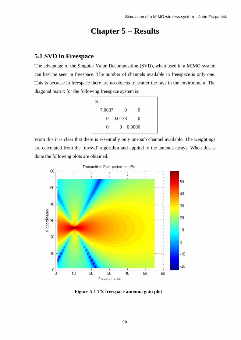
CHAPTER 5 – RESULTS .................................................................................................. 46
5.1 SVD IN FREESPACE ...................................................................................................... 46
iv5.2 NUMBER OF ELEMENTS IN AN ARRAY............................................................................ 49

Simulation of a MIMO wireless system – John Fitzpatrick
5.3 DIELECTRIC PARAMETERS AND CORRIDOR MODEL........................................................ 51
CHAPTER 6 - CONCLUSIONS AND FURTHER RESEARCH................................... 55
Matlab code for Beamforming....................................................................................... 58
C++ Gaussian Elimination Code.................................................................................. 60
Matlab Singular Value Decomposition (SVD) Code..................................................... 64
Matlab ‘mimo’ Code...................................................................................................... 66
v

Simulation of a MIMO wireless system – John Fitzpatrick
Table of Figures
FIGURE 2-1 MULTIPATH ENVIRONMENT ........................................................................ 3 FIGURE 2-2 SIMO SYSTEM............................................................................................. 5 FIGURE 2-3 LINEAR BEAMFORMING ARRAY................................................................... 6 FIGURE 2-4 BEAMFORMING ............................................................................................ 7 FIGURE 2-5 THREE ELEMENT MIMO SYSTEM................................................................. 8 FIGURE 2-6 DATA TRANSMISSION IN MIMO SYSTEMS ................................................... 8 FIGURE 3-1 BUILDING STRUCTURE............................................................................... 15 FIGURE 3-2 OBLONG (WALL) ....................................................................................... 16 FIGURE 3-3 FACE.......................................................................................................... 17 FIGURE 3-4 RAY NODES ............................................................................................... 19 FIGURE 3-5 DIRECT RAY .............................................................................................. 20 FIGURE 3-6 FIRST ORDER IMAGE.................................................................................. 21 FIGURE 3-7 FINDING REFLECTION POINTS.................................................................... 22 FIGURE 3-8 FINDING THE REFLECTION POINT................................................................ 25 FIGURE 3-9 SAMPLE POINTS FOR CONVERGENCE .......................................................... 27 FIGURE 3-10 CONVERGENCE GRAPH, BLUE =1ST, RED =2ND, GREEN 3RD ORDER ........... 27 FIGURE 3-11 2D PLOT OF 4TH ORDER ROOM WITH 6 WALLS ......................................... 28 FIGURE 3-12 3D PLOT OF 4TH ORDER ROOM WITH 6 WALLS ......................................... 29 FIGURE 4-1 SCREENSHOT OF GAUSSIAN ELIMINATION PROGRAM................................. 32 FIGURE 4-2 SCREENSHOT OF C++ SVD PROGRAM ....................................................... 34 FIGURE 4-3 SCREENSHOT OF RAY TRACING PROGRAM.................................................. 43 FIGURE 4-4 SCREENSHOT “PLEASE ENTER ORDER” ...................................................... 43 FIGURE 4-5 SCREENSHOT “PLEASE RUN ‘MYSVD’ ” ...................................................... 44 FIGURE 4-6 SCREENSHOT “PLEASE RUN ‘MIMO’“ ......................................................... 44 FIGURE 4-7 RESULT OF RAY TRACING PROGRAM, TX ANTENNA IN FREESPACE............. 45 FIGURE 4-8 RESULT OF RAY TRACING PROGRAM, RX ANTENNA IN FREESPACE ............ 45 FIGURE 5-1 TX FREESPACE ANTENNA GAIN PLOT ......................................................... 46 FIGURE 5-2 RX FREESPACE ANTENNA GAIN PLOT......................................................... 47 FIGURE 5-3 TX FREESPACE ANTENNA GAIN PLOT WITH ANTENNA SHIFTED UP ............. 48 FIGURE 5-4 RX FREESPACE ANTENNA GAIN PLOT WITH ANTENNA SHIFTED UP ............. 48 FIGURE 5-5 3 ELEMENT ANTENNA ARRAY..................................................................... 49 FIGURE 5-6 5 ELEMENT ANTENNA ARRAY..................................................................... 50 FIGURE 5-7 7 ELEMENT ANTENNA ARRAY..................................................................... 50 FIGURE 5-8 TX CORRIDOR MODEL................................................................................ 52 FIGURE 5-9 RX CORRIDOR MODEL................................................................................ 52
vi

Simulation of a MIMO wireless system – John Fitzpatrick
FIGURE 5-10 TX CORRIDOR MODEL, INCREASED DIELECTRIC PARAMETERS ................. 53 FIGURE 5-11 RX CORRIDOR MODEL, INCREASED DIELECTRIC PARAMETERS ................. 54
vii
Simulation of a MIMO wireless system – John Fitzpatrick
Chapter 1 - Introduction
In the modern era of communications, the ability to send large volumes of data is crucial.
With the increasing use of wireless LAN technology and third generation mobile telephony
systems, the demand for data services has never been greater. The bandwidth of wireless
communication systems is often limited by the cost of the radio spectrum required. Any
increase in bit rate, which can be realised without increasing the bandwidth, makes the
system more spectrally efficient and less costly. Traditional wireless communication
systems have been made more spectrally efficient through the use of clever coding
techniques and algorithms. However, the fundamental bandwidth limitation does not change.
Multiple Input Multiple Output (MIMO) communication systems have been an increasingly
hot topic of research over the past eight years, due to their ability to greatly increase spectral
efficiencies.
As opposed to traditional wireless systems, in which there is one transmitting and one
receiving antenna, MIMO systems use arrays of multiple antennas at both ends of the
communication link, all operating at the same frequency at the same time. This introduces
spatial diversity into the system, which can be used to tackle the problem of multipath. In
wireless communications system, such as point to point radio links, radio waves do not
simply propagate from the transmit antenna to the receive antenna. Rather they bounce and
scatter off objects, this effect is known as multipath. This effect is regarded as an
impediment to the accurate transmission of data in traditional wireless links. MIMO systems
exploit multipath by using the rich scattering environment to increase the spectral efficiency
of the wireless system.
The modelling of radio waves on a large scale can be very complex. There is however, a
simplification. At high frequencies radio waves can be approximated as travelling along
localized paths. This is similar to the geometrical treatment of light rays in optics. Using ray
tracing methods, complex radio environments can be modelled.
The use of numerical techniques is crucial to the operation of MIMO systems. Algorithms
and signal processing at both ends of a MIMO wireless link are crucial to encode and
1

Simulation of a MIMO wireless system – John Fitzpatrick
decode the data. The most important numerical method in MIMO systems is Singular Value
Decomposition (SVD). This allows the complex path, which exists between transmitter and
receiver to be analysed and simplified.
By combining the above techniques it was the aim of this project to develop a fully
operational MIMO simulator. The simulator needed to model indoor radio environments and
be easy to use.
Chapter 2 - Technical Background
2
Simulation of a MIMO wireless system – John Fitzpatrick
In wireless communications system, such as point to point radio links, radio waves do not
simply propagate from the transmit antenna to the receive antenna. Rather they bounce and
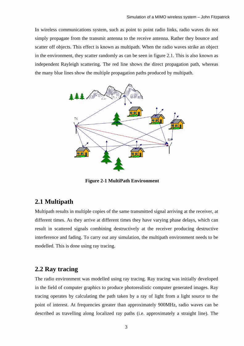
scatter off objects. This effect is known as multipath. When the radio waves strike an object
in the environment, they scatter randomly as can be seen in figure 2.1. This is also known as
independent Rayleigh scattering. The red line shows the direct propagation path, whereas
the many blue lines show the multiple propagation paths produced by multipath.
Figure 2-1 MultiPath Environment
2.1 Multipath Multipath results in multiple copies of the same transmitted signal arriving at the receiver, at
different times. As they arrive at different times they have varying phase delays, which can
result in scattered signals combining destructively at the receiver producing destructive
interference and fading. To carry out any simulation, the multipath environment needs to be
modelled. This is done using ray tracing.
2.2 Ray tracing The radio environment was modelled using ray tracing. Ray tracing was initially developed
in the field of computer graphics to produce photorealistic computer generated images. Ray
tracing operates by calculating the path taken by a ray of light from a light source to the
point of interest. At frequencies greater than approximately 900MHz, radio waves can be
described as travelling along localized ray paths (i.e. approximately a straight line). The
3
Simulation of a MIMO wireless system – John Fitzpatrick
reasoning behind treating the waves as having linear trajectories stems from Maxwell’s
equations.
At high frequencies a more simple method can be used for handling electromagnetics. These
are known as asymptotic methods, more specifically Lumberg-Kline asymptotic expansions.
These are methods of simplification for the solution to Maxwell’s equations.
∑∞
=−≈
0)(
)()(),(
n nnrjf
jrHerH
ωω ψ
∑∞
=−≈
0)(
)()(
),(n n
nrjf
jrE
erEω
ω ψ
Most of the variables in these equations such as the phase function part are of very
complicated and I did not delve into their origin. Asymptotic methods are methods for
expanding functions, evaluating integrals, and solving differential equations, which become
increasingly accurate as some parameter approaches a limiting value [12]. The term of
interest is the frequency term ω . As the frequency approaches zero, only the first term of
the summation of both the electric field and magnetic field remain. This first term is called
the geometrical optics field as it encompasses the classical geometric optics field
characteristics [12]. Using the first term, the geometrical optics field, it can be shown how it
behaves as a ray, which is infinitesimal in width. I did not go into any more detail on this but
for further information please see the noted reference.
For this reason ray tracing can be used as a method for the simulation and approximation of
radio wave propagation at high frequencies. The ray tracing of radio waves operates in the
same manner as optical ray tracing, where transmitters replace light sources and the points
of interest are the receivers.
2.3 Beamforming One solution to the problem of Multipath is to use directional antennas with a single antenna
at either end. Though these will only work if both ends of the link are static, if the receiver
or transmitter is mobile then motor driven directional antennas to rotate the transmitter can
4
Simulation of a MIMO wireless system – John Fitzpatrick
be used. However this is not very practical on a small scale. Another solution is to use
multiple antennas at either the transmitting or receiving end of a link, to accomplish what is
known as beamforming. Beamforming techniques were originally developed for
applications in radar and sonar systems. Using multiple antennas introduces spatial diversity
into the system. These antennas are also known as ‘smart antennas’. Spatial diversity is
based upon the fact that two signals detached in space exhibit independent fading in the
radio channel [3].
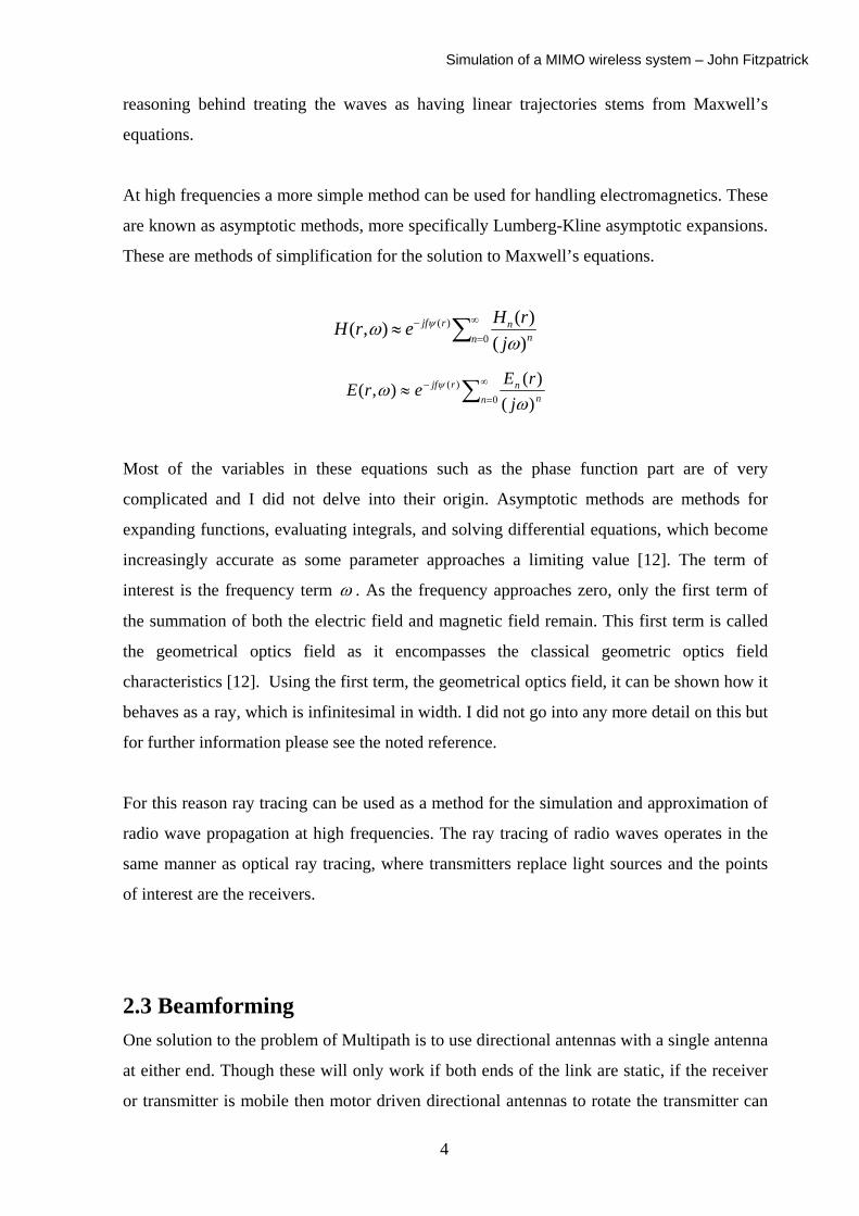
Figure 2.2 below, shows a smart antenna system with multiple antennas at one end of the
link. These systems are also known as SIMO (single-input multiple output). Originally
multiple antennas were placed at the receivers to introduce spatial diversity. This proved to
be too costly and inefficient and the multiple antennas were then placed at the transmitters.
Figure 2-2 SIMO System
Figure 2.2 above, shows a SIMO system operating in a simple modelled room with six
walls. In this case there is one transmitting antenna and three receive antennas. The idea
behind this system is that the probability of not being able to successfully detect a signal,
due to destructive interference, decreases exponentially with the number of antennas used in
a linear array.
5
Simulation of a MIMO wireless system – John Fitzpatrick
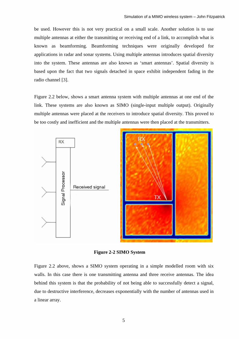
2.4 Linear arrays Beamforming can be accomplished by using many different types of arrays, such as linear,
circular and planar arrays. I will only be considering linear arrays as shown in figure 2.3.
The principal behind beamforming is to introduce different power and phase weightings to
each of the antennas in the array. This is done in such a way as to generate constructive
interference in the desired direction.
Figure 2-3 Linear Beamforming Array
A linear array is shown in figure 2.3, the elements are uniformly spaced with spacing d. It
shows a wave incident on the array at an angleθ , with respect to the normal. The wave
arrives earlier at element 2 than at element 0 or 1. The distance between each element is
given by θsind , and therefore the phase delay between two adjacent elements will be the
time it takes the incident wave to travel the extra distance. The spacing between the
elements must be large enough so as to achieve independent fading. If they are not
appropriately spaced, there will be a loss in spatial diversity.
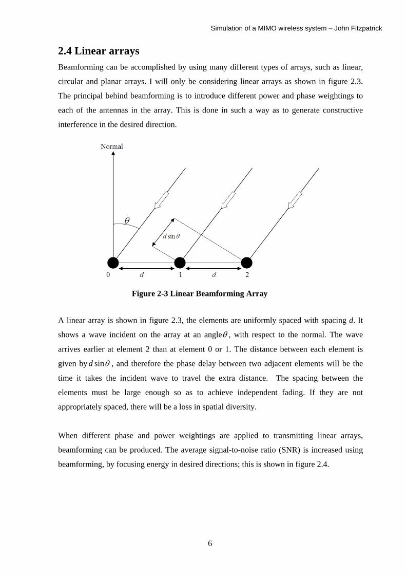
When different phase and power weightings are applied to transmitting linear arrays,
beamforming can be produced. The average signal-to-noise ratio (SNR) is increased using
beamforming, by focusing energy in desired directions; this is shown in figure 2.4.
6
Simulation of a MIMO wireless system – John Fitzpatrick
Figure 2-4 Beamforming
As is seen in the above figure, the different applied weightings result in destructive and
constructive interference in such a way so as to create a main lobe of constructive
interference in a particular direction, this is known as the directivity. This plot was obtained
using the Matlab code in appendix 1. This effect can also be implemented at the receiver end
of a link by phasing and weighting the received signals. However, in severe multipath
environments, beamforming will no longer be effective, as the signals are too severely
scattered to be effectively recovered.
2.5 MIMO MIMO exploits multipath, traditionally a pitfall in wireless communications, to enhance
rather than degrade the signal. MIMO systems consist of multiple transmitters and multiple
receivers. For MIMO systems to be most effective, a rich multipath scattering environment
is needed to create independent propagation channels. It is the rich scattering in the
propagation channel, which offers multiple parallel sub channels at the same frequency,
therefore giving higher capacities over the same bandwidth.
7
Simulation of a MIMO wireless system – John Fitzpatrick
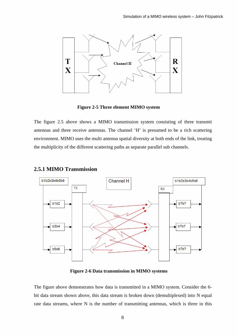
Figure 2-5 Three element MIMO system
The figure 2.5 above shows a MIMO transmission system consisting of three transmit
antennas and three receive antennas. The channel ‘H’ is presumed to be a rich scattering
environment. MIMO uses the multi antenna spatial diversity at both ends of the link, treating
the multiplicity of the different scattering paths as separate parallel sub channels.
2.5.1 MIMO Transmission
Figure 2-6 Data transmission in MIMO systems
The figure above demonstrates how data is transmitted in a MIMO system. Consider the 6-
bit data stream shown above, this data stream is broken down (demultiplexed) into N equal
rate data streams, where N is the number of transmitting antennas, which is three in this
8
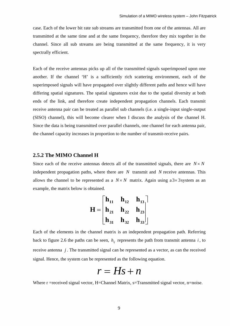
Simulation of a MIMO wireless system – John Fitzpatrick
case. Each of the lower bit rate sub streams are transmitted from one of the antennas. All are
transmitted at the same time and at the same frequency, therefore they mix together in the
channel. Since all sub streams are being transmitted at the same frequency, it is very
spectrally efficient.
Each of the receive antennas picks up all of the transmitted signals superimposed upon one
another. If the channel ‘H’ is a sufficiently rich scattering environment, each of the
superimposed signals will have propagated over slightly different paths and hence will have
differing spatial signatures. The spatial signatures exist due to the spatial diversity at both
ends of the link, and therefore create independent propagation channels. Each transmit
receive antenna pair can be treated as parallel sub channels (i.e. a single-input single-output
(SISO) channel), this will become clearer when I discuss the analysis of the channel H.
Since the data is being transmitted over parallel channels, one channel for each antenna pair,
the channel capacity increases in proportion to the number of transmit-receive pairs.
2.5.2 The MIMO Channel H Since each of the receive antennas detects all of the transmitted signals, there are NN ×
independent propagation paths, where there are transmit and receive antennas. This
allows the channel to be represented as a
N N
NN × matrix. Again using a system as an
example, the matrix below is obtained.
33×
⎥⎥⎥
⎦
⎤
⎢⎢⎢
⎣
⎡=
333231
232221
131211
hhhhhhhhh
H
Each of the elements in the channel matrix is an independent propagation path. Referring
back to figure 2.6 the paths can be seen, represents the path from transmit antenna i , to
receive antenna . The transmitted signal can be represented as a vector, as can the received
signal. Hence, the system can be represented as the following equation.
ijh
j
nHsr +=
Where r =received signal vector, H=Channel Matrix, s=Transmitted signal vector, n=noise.
9
Simulation of a MIMO wireless system – John Fitzpatrick
The transmitted signals in the vector r are complex signals, as are the channel matrix values
and the received signals in vector s. The complex form in each of the elements in the vectors
represents the power of the signal and its phase delay. The complex form of the elements of
the channel matrix ‘H’ represent the attenuation and phase delay associated with that
propagation path. The next step is to look at how the received signal can be decoded.
2.6 Gaussian Elimination Gaussian elimination is a method, which can be used to determine at the receiver, what
signal was transmitted. From the previous section the system equation is known.
Ignoring any noise in the channel, for the sake of simplification, the system equation
simplifies to . This states that the received signal is equal to the transmitted signal
multiplied by the channel matrix. In this case it is presumed that the receiver has full
knowledge of the channel properties and hence knows the channel matrix.
nHsr +=
Hsr =
Gaussian elimination is a systematic approach used to solve sets of linear equations. The
process works by reducing the equations to triangular form as they can be more easily
solved using back substitution. Back substitution is simply the formal name given to the
way one would solve the equations by hand.
As an example consider the following triangular system.
8253 321 =++ xxx ……………. (1)
728 32 −=+ xx ……………. (2)
36 3 =x ……………. (3)
Equation (3) gives 21
63
3 ==x
Using back substitution of into equation (2) gives, 3x
1)27(81
32 −=−−= xx
Again using back substitution into equation (1) gives,
4)258(31
321 =−−= xxx
10
Simulation of a MIMO wireless system – John Fitzpatrick
As can be seen triangular systems can be very easily solved. The problem is reducing a set
of linear equations to triangular form. This is done using by a method called pivoting, which
reorganizes the equations to eliminate some of the variables. Pivoting is best explained with
an example.
As an example consider the following system
728 32 −=+ xx
8253 321 =++ xxx
26826 321 =++ xxx
These equations must be reorganized to obtain a pivot equation. This will allow to be
eliminated for one of the equations. So reorganizing gives,
1x
8253 321 =++ xxx
728 32 −=+ xx
26826 321 =++ xxx
The next step is elimination of from the third equation. The matrix shown on the left
below is the augmented matrix.
1x
1x can be eliminated from the third equation by subtracting 36 times the pivot equation from
the third equation. This will give the following result.
This gives a new pivot equation and the same principle as previous can be applied. Here
can be eliminated by subtracting 2x 188
−=− times the pivot equation. Then the system is in
triangular form.
8253 321 =++ xxx
728 32 −=+ xx
11
Simulation of a MIMO wireless system – John Fitzpatrick
36 3 =x
These can then be solved using the back substitution method as discussed earlier.
I wrote a program in C++, which performs Gaussian elimination with both complex and real
numbers. This is discussed and shown in detail in the chapter ‘implementation of MIMO
simulator’.
The problem with Gaussian elimination is that if the matrices are singular or very close to
singular, then a pivot equation cannot be established.
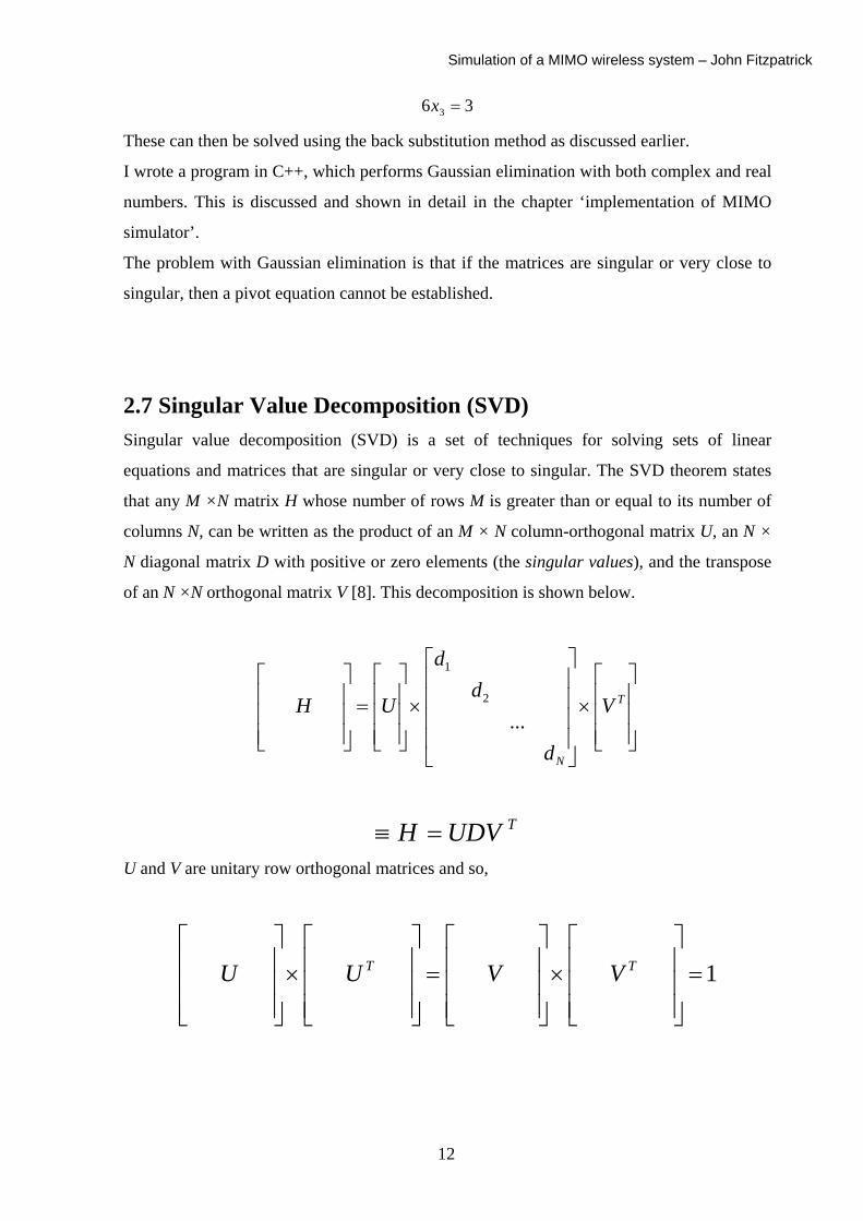
2.7 Singular Value Decomposition (SVD) Singular value decomposition (SVD) is a set of techniques for solving sets of linear
equations and matrices that are singular or very close to singular. The SVD theorem states
that any M ×N matrix H whose number of rows M is greater than or equal to its number of
columns N, can be written as the product of an M × N column-orthogonal matrix U, an N ×
N diagonal matrix D with positive or zero elements (the singular values), and the transpose
of an N ×N orthogonal matrix V [8]. This decomposition is shown below.
⎥⎥⎥
⎦
⎤
⎢⎢⎢
⎣
⎡×
⎥⎥⎥⎥
⎦
⎤
⎢⎢⎢⎢
⎣
⎡
×⎥⎥⎥
⎦
⎤
⎢⎢⎢
⎣
⎡=
⎥⎥⎥
⎦
⎤
⎢⎢⎢
⎣
⎡T
N
V
d
dd
UH...
2
1
TUDVH =≡
U and V are unitary row orthogonal matrices and so,
1=⎥⎥⎥
⎦
⎤
⎢⎢⎢
⎣
⎡×⎥⎥⎥
⎦
⎤
⎢⎢⎢
⎣
⎡=
⎥⎥⎥
⎦
⎤
⎢⎢⎢
⎣
⎡×⎥⎥⎥
⎦
⎤
⎢⎢⎢
⎣
⎡TT VVUU
12
Simulation of a MIMO wireless system – John Fitzpatrick
SVD can be used to decompose the MIMO channel matrix H into a set of equivalent single-
input single-output (SISO) channels. Using the system equation established earlier
, and using the results of the SVD, the system equation can be rewritten as, nHsr +=
nsUDVr T +=
For the sake of simplicity the noise in the system is ignored. Hence,
sUDVr T=
sUDVUrU TTT =
Since U and V are orthogonal,
sDVrU TT =
Let rUr T=~ and sVs T=~ , therefore the system equation becomes
sDr ~~ =
Since D is a diagonal matrix, this represents the system as equivalent parallel SISO
channels.
The advantage of this is that the values of the diagonal matrix D determine the number of
independent parallel channels available in the channel H. This is given by the number of
non-zero eigenvalues, each of these gives the rank of that particular sub channel. Also the
values obtained from the orthogonal matrices of the SVD gives the gains of the independent
channels. These can be used to find weightings for the transmitting and receiving antennas.
This creates beamforming as seen earlier and greatly increases the system performance. I
will discuss this in greater detail in a later section.
Chapter 3 – Implementation of Ray Tracing
13
Simulation of a MIMO wireless system – John Fitzpatrick
3.1 Ray tracing The radio environment was modelled using ray tracing. Ray tracing was initially developed
in the field of computer graphics to produce photorealistic computer-generated images. Ray
tracing operates by calculating the path taken by a ray of light, from a light source to the
point of interest.
At frequencies greater than approximately 900MHz, radio waves can be described as
travelling along localized ray paths (i.e. approximately a straight line). Therefore, ray
tracing can be used as a method for the simulation and approximation of radio wave
propagation. The ray tracing of radio waves operates in the same manner as optical ray
tracing, where light sources are replaced by transmitters and the points of interest are the
receivers.
3.1.2 The ray tracing program To simulate an indoor radio environment the geometry of the environment must be
determined. At the beginning of the project I was given a ray tracing program, which could
handle up to second order reflections, for a single antenna, single receiver system, with no
specific weighting applied. The program was written in C++ and Matlab is used to plot the
results of the ray tracing. For the ray tracing program to be used for multiple input multiple
output systems the program needed to be modified. The modifications needed were as
follows:
• perform calculations for up to Nth order reflections,
• use multiple antennas and multiple receivers,
• apply weighting to both the receiver and transmitter.
C++ is an object oriented programming language. This meant that modifying and adding to
the code was simplified as the program was well structured in a logical format.
The program uses objects to represent the different aspects of the system. These were
represented in classes containing the constructors and functions for each object. The
program calculates the power level at every point in the environment, how it does this will
be explained later. These assigned power values are in dBs, and can then be plotted in
MATLAB. I will now go through the different objects of the system and describe how each
functions.
14
Simulation of a MIMO wireless system – John Fitzpatrick
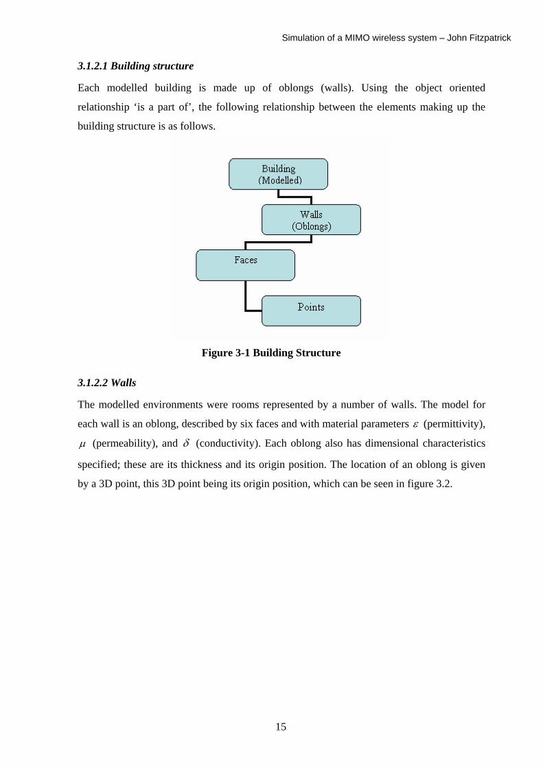
3.1.2.1 Building structure
Each modelled building is made up of oblongs (walls). Using the object oriented
relationship ‘is a part of’, the following relationship between the elements making up the
building structure is as follows.
Figure 3-1 Building Structure
3.1.2.2 Walls
The modelled environments were rooms represented by a number of walls. The model for
each wall is an oblong, described by six faces and with material parameters ε (permittivity),
µ (permeability), and δ (conductivity). Each oblong also has dimensional characteristics
specified; these are its thickness and its origin position. The location of an oblong is given
by a 3D point, this 3D point being its origin position, which can be seen in figure 3.2.
15
Simulation of a MIMO wireless system – John Fitzpatrick
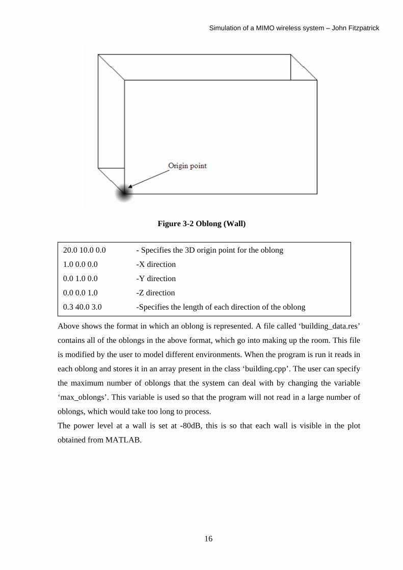
Figure 3-2 Oblong (Wall)
A
c
i
e
t
‘
o
T
o
20.0 10.0 0.0 - Specifies the 3D origin point for the oblong
1.0 0.0 0.0 -X direction
0.0 1.0 0.0 -Y direction
0.0 0.0 1.0 -Z direction
0.3 40.0 3.0 -Specifies the length of each direction of the oblong
bove shows the format in which an oblong is represented. A file called ‘building_data.res’
ontains all of the oblongs in the above format, which go into making up the room. This file
s modified by the user to model different environments. When the program is run it reads in
ach oblong and stores it in an array present in the class ‘building.cpp’. The user can specify
he maximum number of oblongs that the system can deal with by changing the variable
max_oblongs’. This variable is used so that the program will not read in a large number of
blongs, which would take too long to process.
he power level at a wall is set at -80dB, this is so that each wall is visible in the plot
btained from MATLAB.
16
Simulation of a MIMO wireless system – John Fitzpatrick
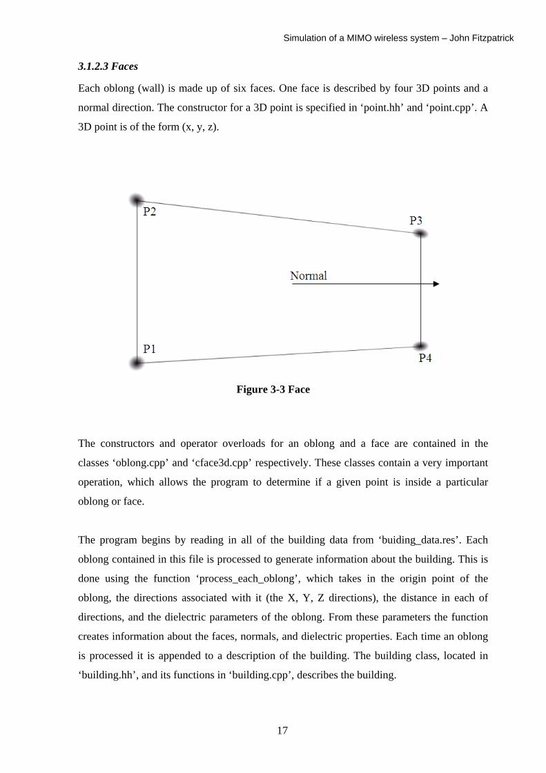
3.1.2.3 Faces
Each oblong (wall) is made up of six faces. One face is described by four 3D points and a
normal direction. The constructor for a 3D point is specified in ‘point.hh’ and ‘point.cpp’. A
3D point is of the form (x, y, z).
Figure 3-3 Face
The constructors and operator overloads for an oblong and a face are contained in the
classes ‘oblong.cpp’ and ‘cface3d.cpp’ respectively. These classes contain a very important
operation, which allows the program to determine if a given point is inside a particular
oblong or face.
The program begins by reading in all of the building data from ‘buiding_data.res’. Each
oblong contained in this file is processed to generate information about the building. This is
done using the function ‘process_each_oblong’, which takes in the origin point of the
oblong, the directions associated with it (the X, Y, Z directions), the distance in each of
directions, and the dielectric parameters of the oblong. From these parameters the function
creates information about the faces, normals, and dielectric properties. Each time an oblong
is processed it is appended to a description of the building. The building class, located in
‘building.hh’, and its functions in ‘building.cpp’, describes the building.
17

Simulation of a MIMO wireless system – John Fitzpatrick
Now the building structure and parameters are known. The program must read in the
locations of the base stations, i.e. the transmitters. The data for the base stations is stored in
the user modifiable file, ‘base_stations.res’, in the following format.
3
30.0 10.0 4.0
30.2 10.0 4.0
The location of each base station is give
the format shown above.
The locations of each base station is read
The original program could not comput
points in the defined environment. The
points (i.e. receiver antennas), to make it
this further later. The specific field
‘receivers.res’, in the same format as
modifications the program can handle m
One of the most essential parts of the r
This function breaks down the room tha
this grid can be set using the value assig
the size being (noc) . The grid takes a
height. Each of these grid points is kno
electric field will be calculated. A field
each field point is simply a 3D coordina
field points, calculating the value of the
field point can be considered as a recei
electric field.
2
-Number of base stations
- Location of 1st base station
- Location of 2nd base station
n by a 3D point of the form (x,y,z) as can be seen in
in and stored in an array called ‘base_stations[]’.
e specified field points; rather it calculated all field
program needed to be able to compute specific field
possible to find the channel matrix H. I will discuss
points are stored in the user modifiable file
the locations of the base stations. With these
ultiple transmitting and multiple receive antennas.
ay tracing program is the ‘contour_fields’ function.
t is being modelled into a grid of points. The size of
ned to the variable ‘noc’ (number of contours), with
2D cross-section through the room at a particular
wn as a field point and is the location at which the
point is described in the class ‘CPoint3d’, where
te. The program then increments through each of the
electric field (magnitude and phase) at each point. A
ver, it is the point in which we are interested in the
18
Simulation of a MIMO wireless system – John Fitzpatrick
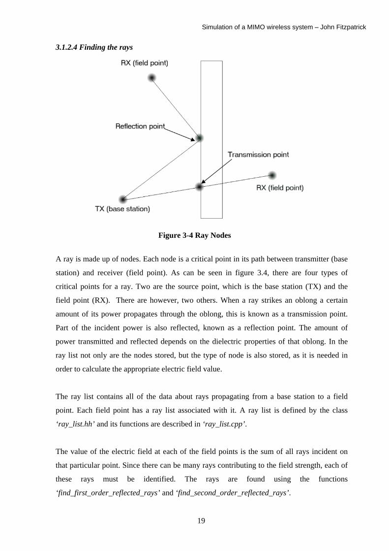
3.1.2.4 Finding the rays
Figure 3-4 Ray Nodes
A ray is made up of nodes. Each node is a critical point in its path between transmitter (base
station) and receiver (field point). As can be seen in figure 3.4, there are four types of
critical points for a ray. Two are the source point, which is the base station (TX) and the
field point (RX). There are however, two others. When a ray strikes an oblong a certain
amount of its power propagates through the oblong, this is known as a transmission point.
Part of the incident power is also reflected, known as a reflection point. The amount of
power transmitted and reflected depends on the dielectric properties of that oblong. In the
ray list not only are the nodes stored, but the type of node is also stored, as it is needed in
order to calculate the appropriate electric field value.
The ray list contains all of the data about rays propagating from a base station to a field
point. Each field point has a ray list associated with it. A ray list is defined by the class
‘ray_list.hh’ and its functions are described in ‘ray_list.cpp’.
The value of the electric field at each of the field points is the sum of all rays incident on
that particular point. Since there can be many rays contributing to the field strength, each of
these rays must be identified. The rays are found using the functions
‘find_first_order_reflected_rays’ and ‘find_second_order_reflected_rays’.
19
Simulation of a MIMO wireless system – John Fitzpatrick
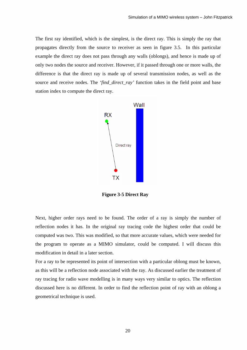
The first ray identified, which is the simplest, is the direct ray. This is simply the ray that
propagates directly from the source to receiver as seen in figure 3.5. In this particular
example the direct ray does not pass through any walls (oblongs), and hence is made up of
only two nodes the source and receiver. However, if it passed through one or more walls, the
difference is that the direct ray is made up of several transmission nodes, as well as the
source and receive nodes. The ‘find_direct_ray’ function takes in the field point and base
station index to compute the direct ray.
Figure 3-5 Direct Ray
Next, higher order rays need to be found. The order of a ray is simply the number of
reflection nodes it has. In the original ray tracing code the highest order that could be
computed was two. This was modified, so that more accurate values, which were needed for
the program to operate as a MIMO simulator, could be computed. I will discuss this
modification in detail in a later section.
For a ray to be represented its point of intersection with a particular oblong must be known,
as this will be a reflection node associated with the ray. As discussed earlier the treatment of
ray tracing for radio wave modelling is in many ways very similar to optics. The reflection
discussed here is no different. In order to find the reflection point of ray with an oblong a
geometrical technique is used.
20
Simulation of a MIMO wireless system – John Fitzpatrick
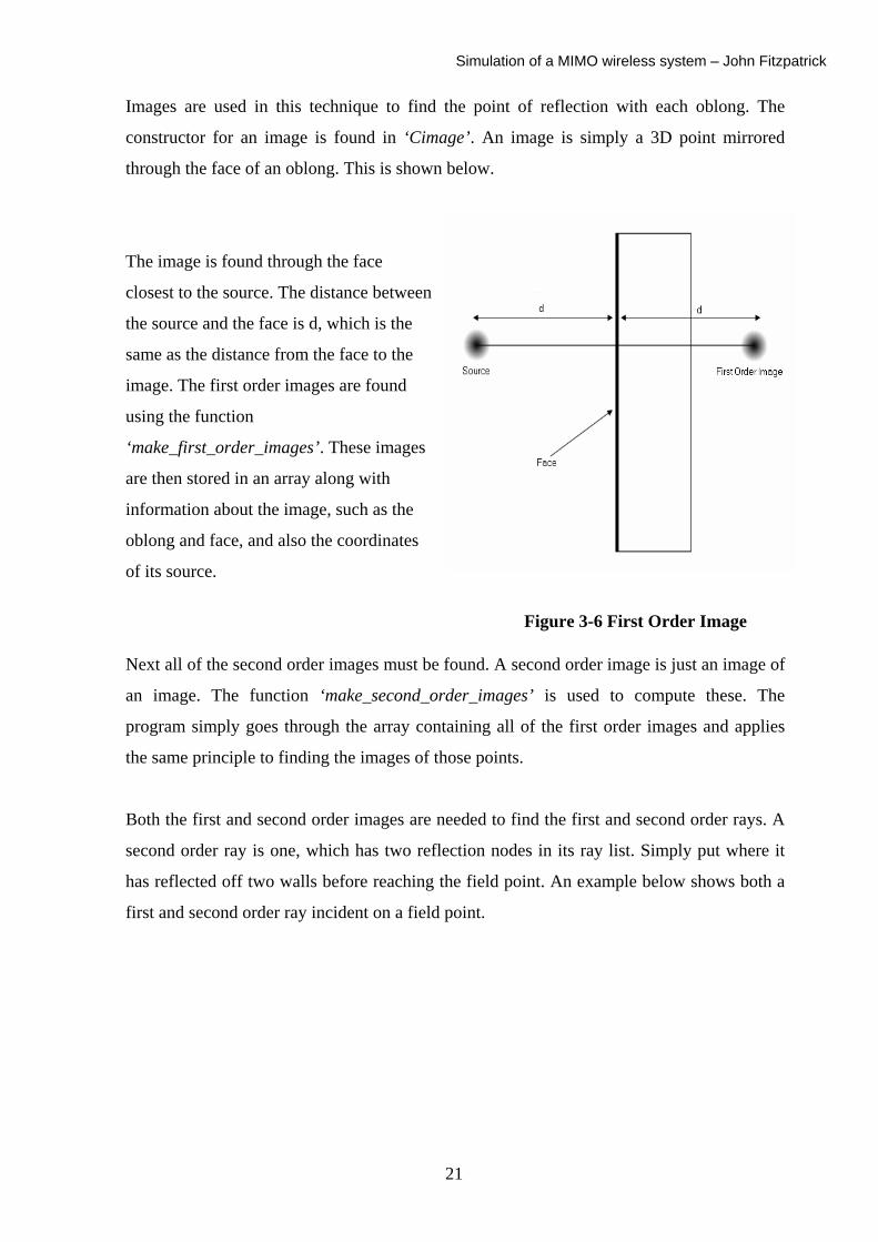
Images are used in this technique to find the point of reflection with each oblong. The
constructor for an image is found in ‘Cimage’. An image is simply a 3D point mirrored
through the face of an oblong. This is shown below.
The image is found through the face
closest to the source. The distance between
the source and the face is d, which is the
same as the distance from the face to the
image. The first order images are found
using the function
‘make_first_order_images’. These images
are then stored in an array along with
information about the image, such as the
oblong and face, and also the coordinates
of its source.
Figure 3-6 First Order Image
Next all of the second order images must be found. A second order image is just an image of
an image. The function ‘make_second_order_images’ is used to compute these. The
program simply goes through the array containing all of the first order images and applies
the same principle to finding the images of those points.
Both the first and second order images are needed to find the first and second order rays. A
second order ray is one, which has two reflection nodes in its ray list. Simply put where it
has reflected off two walls before reaching the field point. An example below shows both a
first and second order ray incident on a field point.
21
Simulation of a MIMO wireless system – John Fitzpatrick
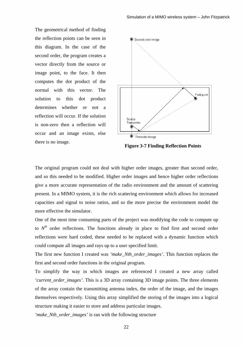
The geometrical method of finding
the reflection points can be seen in
this diagram. In the case of the
second order, the program creates a
vector directly from the source or
image point, to the face. It then
computes the dot product of the
normal with this vector. The
solution to this dot product
determines whether or not a
reflection will occur. If the solution
is non-zero then a reflection will
occur and an image exists, else
there is no image. Figure 3-7 Finding Reflection Points
The original program could not deal with higher order images, greater than second order,
and so this needed to be modified. Higher order images and hence higher order reflections
give a more accurate representation of the radio environment and the amount of scattering
present. In a MIMO system, it is the rich scattering environment which allows for increased
capacities and signal to noise ratios, and so the more precise the environment model the
more effective the simulator.
One of the most time consuming parts of the project was modifying the code to compute up
to Nth order reflections. The functions already in place to find first and second order
reflections were hard coded, these needed to be replaced with a dynamic function which
could compute all images and rays up to a user specified limit.
The first new function I created was ‘make_Nth_order_images’. This function replaces the
first and second order functions in the original program.
To simplify the way in which images are referenced I created a new array called
‘current_order_images’. This is a 3D array containing 3D image points. The three elements
of the array contain the transmitting antenna index, the order of the image, and the images
themselves respectively. Using this array simplified the storing of the images into a logical
structure making it easier to store and address particular images.
‘make_Nth_order_images’ is ran with the following structure
22
Simulation of a MIMO wireless system – John Fitzpatrick
“void make_Nth_order_images(int N, int base_station_index)”
When run, it loads the first transmitter location from base station index and sets it as a zero
order image. current_order_images[base_station_index][0][0]=base_stations[b
ase_station_index]
This is done because images that are currently being calculated need to know the location of
the previous order image, since images of orders greater than one are an image of an image,
as seen previously. For this purpose a temporary array called ‘previous_order_images’ was
created to store the image values while the next higher order images are being calculated.
The function works by iterating using a ‘for’ loop through all images up to the user specified
limit N. At the beginning of this loop the following line is used, previous_order_images[index]=current_order_images[base_station_inde
x][y-1][index]
This stores all of the current order images to the temporary array previous order images. In
the case of the first iteration of the loop, these images will be the base station locations.
Another array ‘current_order_images_count’ stores the number of images for each of the
current orders. In the case of the first iteration it will be the number of images for a
particular base station. The value in this array is used to know how many images exist for a
particular order. Due to the complexity of the calculations and the number of images
generated, an upper limit on the number of images is specified in ‘max_order’. A control
loop checks ‘max_order’ after every iteration to make sure it has not exceeded the
predefined limit. If the limit is reached, the program moves on to the next order. This is done
so as to control the computational time and computer resources used by the program.
The function finds the image of the current order images through each face of each oblong.
The object oriented structure of the program, where a face is part of an oblong etc. made this
easier than it would have otherwise been. The following segment of code shows how this is
achieved.
//Iterate for every Oblong
for( counter = 0 ; counter < 6 ; counter ++)
{
//Iterate for each of the 6 Faces in an Oblong
the_face = the_building.listoblong(i).face(counter) ;
23
Simulation of a MIMO wireless system – John Fitzpatrick
v = previous_order_images[j].listpoint() - the_face.p1() ;
component = v*the_face.normal() ; //perpendicular distance
from Oblong
if(component>0.0) //if the image point lies infront of
face
{
current_order_images[base_station_index][y][image_count] =
CImage(previous_order_images[j].listpoint() -
the_face.normal()*(2.0*component),i,counter,y,j ) ;
This piece of code iterates through each oblong and each face of each oblong. The limit on
the loop is set to six as each oblong has six faces. Once a particular face is selected the
program then creates a vector from the current point being considered. In the first iteration
this is a base station, to the origin point of the face. The origin point can be seen as p1 in
figure 3.2. As seen before, the program then computes the dot product of the vector with the
normal of the face. This gives a value component. If the value of this component is non-zero
then the image exists, and the value of the component is the perpendicular distance from the
point to the face. The next line of code looks very complicated but it simply finds the image
point through the face. It does this by computing the image, which is twice the perpendicular
distance (component) from the point of interest, perpendicularly through the wall. The
program then stores this image point in the ‘current_order_images’ array.
Once all of the images are known the next step is finding the rays. As with finding the
images, the code in the original program was hard coded to compute the first and second
order rays. Here two new functions needed to be created ‘find_nth_order_reflected_rays’
and ‘create_nth_order_reflected_rays’. The major functionality is in
‘create_nth_order_reflected_rays’, ‘find_nth_order_reflected_rays’ basically acts as a
control loop iterating for each image and order, and calling
‘create_nth_order_reflected_rays’ within each iteration.
This function is called in the following manner: create_N_order_reflection_ray(current_order_images[base_statio
n_index][k][i] , field_pt ,base_station_index,k);
24
Simulation of a MIMO wireless system – John Fitzpatrick
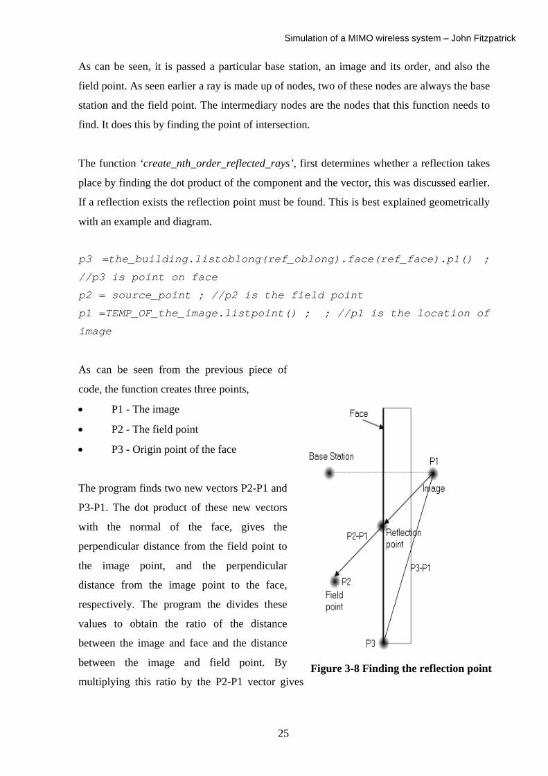
As can be seen, it is passed a particular base station, an image and its order, and also the
field point. As seen earlier a ray is made up of nodes, two of these nodes are always the base
station and the field point. The intermediary nodes are the nodes that this function needs to
find. It does this by finding the point of intersection.
The function ‘create_nth_order_reflected_rays’, first determines whether a reflection takes
place by finding the dot product of the component and the vector, this was discussed earlier.
If a reflection exists the reflection point must be found. This is best explained geometrically
with an example and diagram.
p3 =the_building.listoblong(ref_oblong).face(ref_face).p1() ;
//p3 is point on face
p2 = source_point ; //p2 is the field point
p1 =TEMP_OF_the_image.listpoint() ; ; //p1 is the location of
image
As can be seen from the previous piece of
code, the function creates three points,
• P1 - The image
• P2 - The field point
• P3 - Origin point of the face
The program finds two new vectors P2-P1 and
P3-P1. The dot product of these new vectors
with the normal of the face, gives the
perpendicular distance from the field point to
the image point, and the perpendicular
distance from the image point to the face,
respectively. The program the divides these
values to obtain the ratio of the distance
between the image and face and the distance
between the image and field point. By
multiplying this ratio by the P2-P1 vector gives Figure 3-8 Finding the reflection point
25
Simulation of a MIMO wireless system – John Fitzpatrick
the distance from the image point to the field point. This vector is added to the image point
P1 to give the coordinates of the reflection point.
When the reflection points are found the ray is computed. A ray containing a reflection point
will be a first order or greater ray. The number of reflections in a ray is equal to the order of
the ray. The ‘analyse_direct’ function is initially used to compute the direct ray from a
transmitter to a field point with no reflections. This function also finds the transmission
points through which each ray passes.
In the case of multiple reflections, the ‘analyse_direct’ function is first used from the base
station to the first point of reflection, and from this point to the next reflection and so on
until the field point is reached. The first ray obtained is the ray from the base station to the
first reflection point, which is stored in ‘s2i’ (source to intersection). The next task is to
compute the ray between two reflection points, since there may be many reflection points
there are many reflection-to-reflection rays. These are stored in array called ‘i2i’
(intersection-to-intersection).
The final ray is the one from the last reflection to the field point, which is stored in ‘i2f’
(intersection-to-field point). Once all these rays are computed the source node and field
point node are they are combined to create the ray, this is done by the function
‘create_N_order_reflection_ray’, this function returns the complete ray from transmitter to
field points.
This explains the full operation of the ray tracing program. There are a few more
modifications that were made but I will explain these when I explain the function of the
overall MIMO simulator program.
3.2 Convergence of order Having modified the program to calculate up to N order reflections, I needed to decide what
order to run most of my simulations. As the order is increased, the complexity of the
problem increases, and hence the computational time required becomes greater. A trade-off
needs to be made between the granularity of the results and the time taken to compute them.
26
Simulation of a MIMO wireless system – John Fitzpatrick
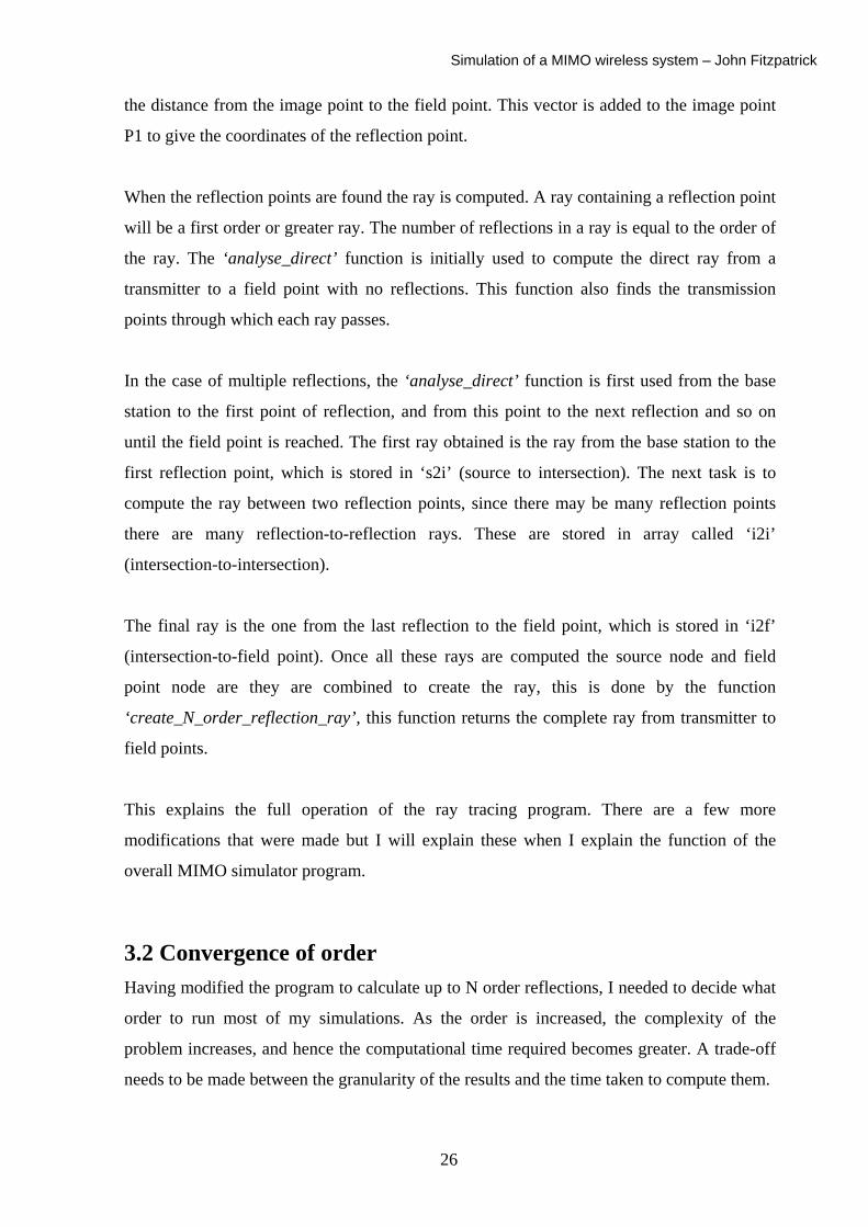
To do this I took a sample of ten field points from the same environment computed to
different orders. The environment modelled is shown here.
Figure 3-9 Sample points for convergence
I then plotted each of the results and overlaid them to see could I obtain any convergence
between orders up to the third order.
Figure 3-10 Convergence graph,
Blue =1st, red =2nd, Green 3rd Order
As can be seen in the graph, the values at the field points begin to converge even after an
order of three. For this reason when modelling most of the environments I used an order of
27
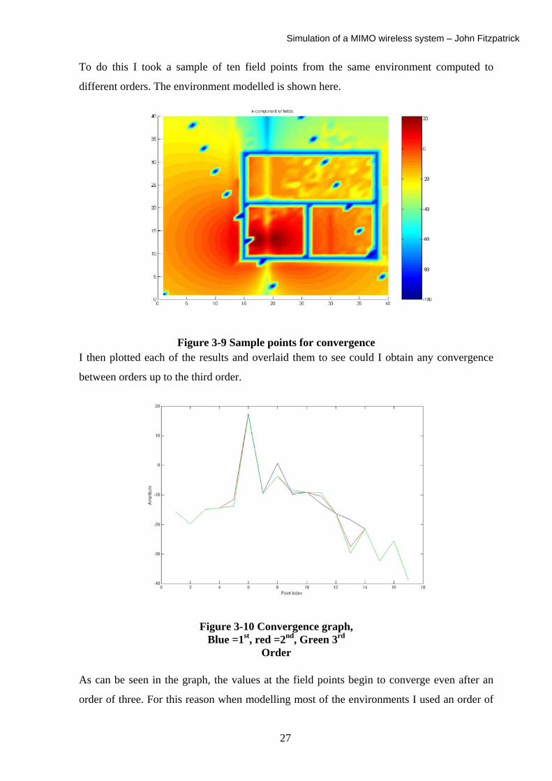
Simulation of a MIMO wireless system – John Fitzpatrick
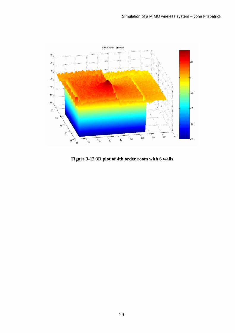
three or four. When computing for orders greater than these the computational time greatly
increases, and the extra accuracy obtained does not justify the extra time. For example, the
following room was modelled for both 4th and 5th order. The 4th order took approximately 3
½ hours on a Pentium 3, but approximately 8 hours for the 5th order.
Figure 3-11 2D plot of 4th order room with 6 walls
28
Simulation of a MIMO wireless system – John Fitzpatrick
Figure 3-12 3D plot of 4th order room with 6 walls
29
Simulation of a MIMO wireless system – John Fitzpatrick
Chapter 4 - Implementation of MIMO Simulator
4.1 Gaussian Elimination As discussed earlier Gaussian elimination is a method that can be used to decode at the
receiver of a MIMO system, the signal which was transmitted. For Gaussian elimination to
work, full channel knowledge needs to be known at the receiver. Put simply the receiver
must know the channel matrix H.
As part of the project I wrote a C++ program, which uses Gaussian elimination on both real
and complex numbers. By inputting the channel matrix and the received signal vector the
program computes the transmitted signal vector. I wrote the program to operate on square
matrices, since the MIMO systems I was trying to simulate had the same number of
transmitters and receivers and hence produces a square channel matrix.
The full source code for the program can be seen in the appendices.
The first thing that must be specified by the user is the size of the square channel matrix.
This is done by changing the value of the integer N. In the main function the user must
specify the channel matrix, as shown below for a 2x2 channel matrix.
The function ‘gauss’ is then
channel matrix is stored in a
in C++ one cannot pass an
element of the array is passe
b[0][0]=complex(-1.265,0.8963);
b[0][1]=complex(1.109,0.1234);
b[1][0]=complex(0.567,-1.64);
called and takes in the channel matrix as a parameter. Since the
n array ‘b’ this must be passed into the function. Unfortunately
array into a function. To pass in the array a pointer to the first
d. The pointer is created as follows.
30
Simulation of a MIMO wireless system – John Fitzpatrick
The ‘gauss’ function takes in the pointer and then creates a temporary array in which it loads
the channel matrix.
The user is then asked to enter the received signal vector, each element of this vector would
be received by one of the receive antennas. This vector is stored in an array called ‘a’. The
vector ‘a’ is attached to the end of the channel matrix, this produces what is known as the
augmented matrix. The augmented matrix has the following form.
⎥⎦
⎤⎢⎣
⎡
132
010
abbabb
The ‘b’ values represent the channel matrix and the ‘a’ values is the received signal vector.
The next step is the elimination step.
In this s
theory o
the code
chapter.
//******perform elimination step
for(int index=0; index<=N; index++)
{
complex pivot;
for(int row=index+1; row<=N-1; row++)
{
pivot = -a[row][index]/a[index][index];
for(int column=index+1; column<=N; column++)
{
//*****Needed to convert 2D array to pointed array
bb=(complex **) malloc((unsigned) N*sizeof(complex*));
for(i=0;i<=N-1;i++) bb[i]=b[i];
tep the pivot equation is found and then used to eliminate the first variable. For the
f how this operates see the technical background chapter. The best way to see how
operates is to follow the steps of the example given in the technical background
This step is iterated until the system is reduced to triangular form.
31
Simulation of a MIMO wireless system – John Fitzpatrick
Then the value obtained by reducing the system to triangular form is then used to solve the
equations. This is done using back substitution as discussed earlier. The algorithm to
perform this is shown below.
I origin
importe
perform
final pr
//*********perform back substitution step.
s[N-1]=a[N-1][N]/a[N-1][N-1];
for (row=N; row>=0; row--)
{
for(int column=N-1; column>=row+1; column--)
{
a[row][N]=s[column]*a[row][column]a[row][N];
}
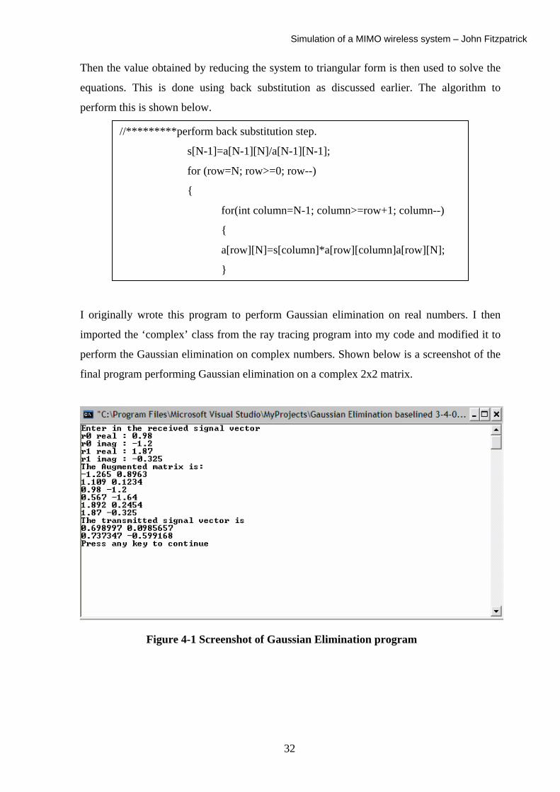
ally wrote this program to perform Gaussian elimination on real numbers. I then
d the ‘complex’ class from the ray tracing program into my code and modified it to
the Gaussian elimination on complex numbers. Shown below is a screenshot of the
ogram performing Gaussian elimination on a complex 2x2 matrix.
Figure 4-1 Screenshot of Gaussian Elimination program
32
Simulation of a MIMO wireless system – John Fitzpatrick
4.2 SVD As previously discussed in the chapter entitled ‘Technical background’, Gaussian
elimination will not work on matrices, which are almost singular. By singular I mean
matrices in which all the elements of the matrix have identical or very similar values. With
some difficulty, I adapted an algorithm from ‘numerical recipes in C’, to perform singular
value decomposition on a square matrix. Although the original algorithm could perform
SVD on any arbitrary size matrix, for the MIMO systems I was simulating, the channel
matrix was always square.
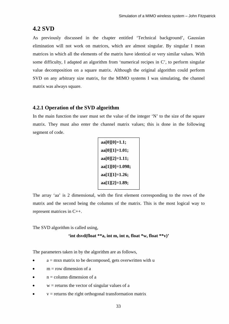
4.2.1 Operation of the SVD algorithm In the main function the user must set the value of the integer ‘N’ to the size of the square
matrix. They must also enter the channel matrix values; this is done in the following
segment of code.
The array ‘aa’ is 2 dimensional, w
matrix and the second being the c
represent matrices in C++.
The SVD algorithm is called using,
‘int dsvd(float *
The parameters taken in by the algo
• a = mxn matrix to be decom
• m = row dimension of a
• n = column dimension of a
• w = returns the vector of sin
• v = returns the right orthogo
aa[0][0]=1.1;
aa[0][1]=1.01;
aa[0][2]=1.11;
aa[1][0]=1.098;
aa[1][1]=1.26;
aa[1][2]=1.89;
ith the first element corresponding to the rows of the
olumns of the matrix. This is the most logical way to
*a, int m, int n, float *w, float **v)’
rithm are as follows,
posed, gets overwritten with u
gular values of a
nal transformation matrix
33
Simulation of a MIMO wireless system – John Fitzpatrick
In the case of the square matrix the value for ‘n’ and ‘m’ are the same and so in the main
function both of these are set equal to the value of the integer ‘N’.
As previously discussed, in C++ an array cannot be passed directly to a function. Rather a
pointer to the first element of the array is passed.
In the main function the following piece of code was used to convert the array to a pointed
memory location.
Since a 2 dime
dimensional (i.e
locations to eac
be the channel m
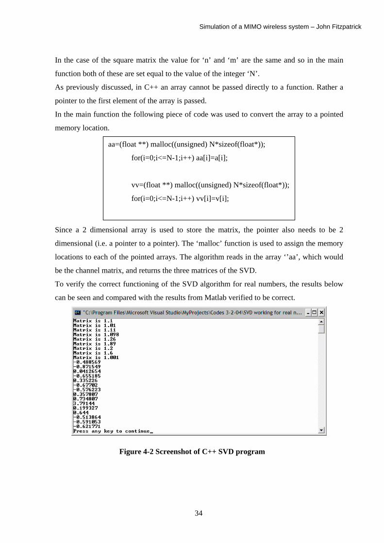
To verify the co
can be seen and
aa=(float **) malloc((unsigned) N*sizeof(float*));
for(i=0;i<=N-1;i++) aa[i]=a[i];
vv=(float **) malloc((unsigned) N*sizeof(float*));
for(i=0;i<=N-1;i++) vv[i]=v[i];
nsional array is used to store the matrix, the pointer also needs to be 2
. a pointer to a pointer). The ‘malloc’ function is used to assign the memory
h of the pointed arrays. The algorithm reads in the array ‘’aa’, which would
atrix, and returns the three matrices of the SVD.
rrect functioning of the SVD algorithm for real numbers, the results below
compared with the results from Matlab verified to be correct.
Figure 4-2 Screenshot of C++ SVD program
34
Simulation of a MIMO wireless system – John Fitzpatrick
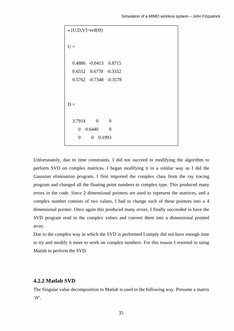
» [U,D,V]=svd(H)
U =
0.4886 -0.0413 0.8715
0.6552 0.6770 -0.3352
0.5762 -0.7348 -0.3578
D =
3.7914 0 0
0 0.6440 0
0 0 0.1993
Unfortunately, due to time constraints, I did not succeed in modifying the algorithm to
perform SVD on complex matrices. I began modifying it in a similar way as I did the
Gaussian elimination program. I first imported the complex class from the ray tracing
program and changed all the floating point numbers to complex type. This produced many
errors in the code. Since 2 dimensional pointers are used to represent the matrices, and a
complex number consists of two values, I had to change each of these pointers into a 4
dimensional pointer. Once again this produced many errors. I finally succeeded in have the
SVD program read in the complex values and convert them into a dimensional pointed
array.
Due to the complex way in which the SVD is performed I simply did not have enough time
to try and modify it more to work on complex numbers. For this reason I resorted to using
Matlab to perform the SVD.
4.2.2 Matlab SVD The Singular value decomposition in Matlab is used in the following way. Presume a matrix
‘H’.
35
Simulation of a MIMO wireless system – John Fitzpatrick
[U,S,V] = SVD(H)
This returns a diagonal matrix S, of the same size as ‘H’, with non negative diagonal
elements in decreasing order. It also returns the unitary matrices U and V. The values
returned are the solutions to the product,
'
Due to the fact that the SVD was no
originally planned, I made some more
MIMO simulator as easy to use as poss
The ray tracing code was modified to c
locations of the receivers from a user m
file is the same as for the base stati
received field strength magnitude and
receivers. The output of each of the tr
phase of zero, and therefore the fie
magnitude and phase distortion over
three transmitter, three receiver syste
corresponds to one transmit receive a
matrix and are written to a file called ‘r
The first task of the Matlab co
matrix. Due to the order in which the
and the format I needed the matrix t
needed.
H = U*S*V
w being implemented in Matlab and not in C++ asmodifications to the C++ program so as to make the
ible.
alculate the channel matrix ‘H’. The code reads in the
odifiable file called ‘receiver.res’. The format of this
on locations file. The channel matrix is simply the
phase, from each of the transmitting antennas at the
ansmitters is normalised to a magnitude of one and a
ld strength at each field point corresponds to the
that particular propagation path. For example for a
m, there will be nine different values. Each value
ntenna pair. These values correspond to the channel
eceived_fields.res’.
de is to read in these values and create the channel
channel matrix is written in the ray tracing program,
o have in Matlab the following piece of code was
36
Simulation of a MIMO wireless system – John Fitzpatrick
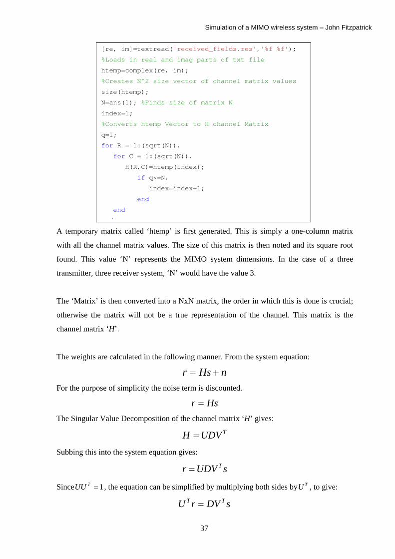
A temporary matrix called ‘htemp’ is first generated. This is simply a one-column matrix
with all the channel matrix values. The size of this matrix is then noted and its square root
found. This value ‘N’ represents the MIMO system dimensions. In the case of a three
transmitter, three receiver system, ‘N’ would have the value 3.
[re, im]=textread('received_fields.res','%f %f');
%Loads in real and imag parts of txt file
htemp=complex(re, im);
%Creates N^2 size vector of channel matrix values
size(htemp);
N=ans(1); %Finds size of matrix N
index=1;
%Converts htemp Vector to H channel Matrix
q=1;
for R = 1:(sqrt(N)),
for C = 1:(sqrt(N)),
H(R,C)=htemp(index);
if q<=N,
index=index+1;
end
end
d
The ‘Matrix’ is then converted into a NxN matrix, the order in which this is done is crucial;
otherwise the matrix will not be a true representation of the channel. This matrix is the
channel matrix ‘H’.
The weights are calculated in the following manner. From the system equation:
nHsr +=
For the purpose of simplicity the noise term is discounted.
Hsr =
The Singular Value Decomposition of the channel matrix ‘H’ gives: TUDVH =
Subbing this into the system equation gives:
sUDVr T= Since , the equation can be simplified by multiplying both sides by , to give: 1=TUU TU
sDVrU TT =
37
Simulation of a MIMO wireless system – John Fitzpatrick
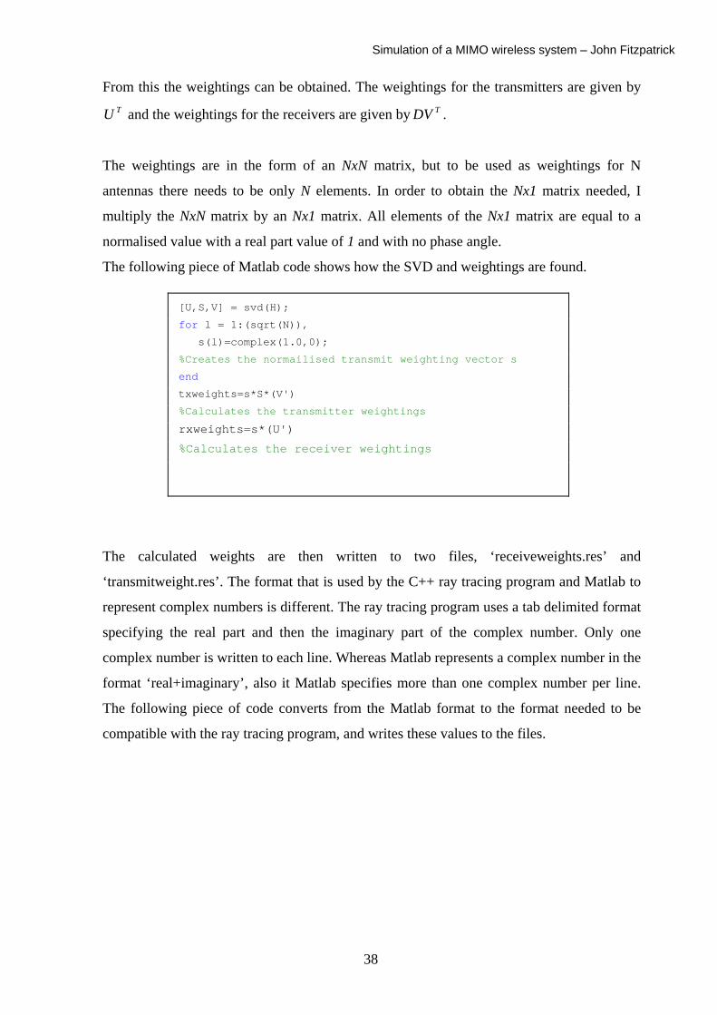
From this the weightings can be obtained. The weightings for the transmitters are given by
and the weightings for the receivers are given by . TU TDV
The weightings are in the form of an NxN matrix, but to be used as weightings for N
antennas there needs to be only N elements. In order to obtain the Nx1 matrix needed, I
multiply the NxN matrix by an Nx1 matrix. All elements of the Nx1 matrix are equal to a
normalised value with a real part value of 1 and with no phase angle.
The following piece of Matlab code shows how the SVD and weightings are found.
[U,S,V] = svd(H);
for l = 1:(sqrt(N)),
s(l)=complex(1.0,0);
%Creates the normailised transmit weighting vector s
end
txweights=s*S*(V')
%Calculates the transmitter weightings
rxweights=s*(U')
%Calculates the receiver weightings
The calculated weights are then written to two files, ‘receiveweights.res’ and
‘transmitweight.res’. The format that is used by the C++ ray tracing program and Matlab to
represent complex numbers is different. The ray tracing program uses a tab delimited format
specifying the real part and then the imaginary part of the complex number. Only one
complex number is written to each line. Whereas Matlab represents a complex number in the
format ‘real+imaginary’, also it Matlab specifies more than one complex number per line.
The following piece of code converts from the Matlab format to the format needed to be
compatible with the ray tracing program, and writes these values to the files.
38
Simulation of a MIMO wireless system – John Fitzpatrick
These calculate
in directions co
the results sect
in more detail.
4.3 FurtheTo make the
simulator, furt
tracing progra
weighting is si
Once the anten
the ray tracing
At this point th
transmitter. If
around the dat
receiver as a tr
ray tracing pro
simultaneously
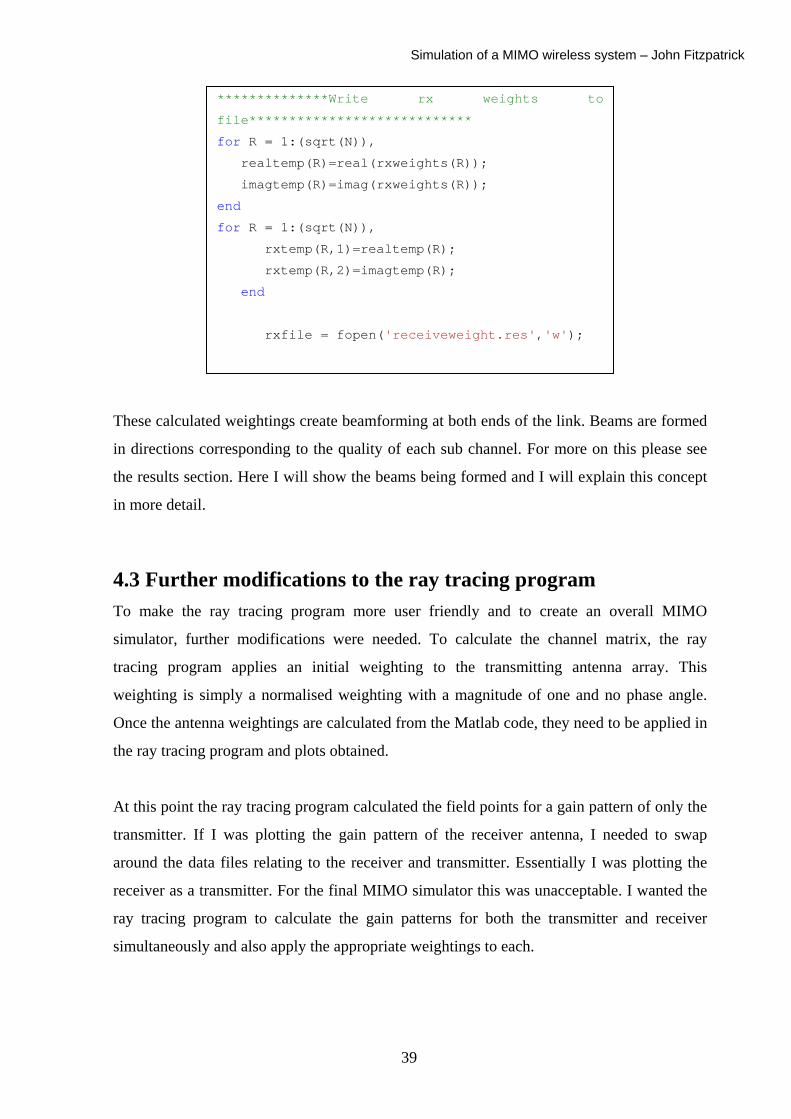
**************Write rx weights to
file****************************
for R = 1:(sqrt(N)),
realtemp(R)=real(rxweights(R));
imagtemp(R)=imag(rxweights(R));
end
for R = 1:(sqrt(N)),
rxtemp(R,1)=realtemp(R);
rxtemp(R,2)=imagtemp(R);
end
rxfile = fopen('receiveweight.res','w');
d weightings create beamforming at both ends of the link. Beams are formed
rresponding to the quality of each sub channel. For more on this please see
ion. Here I will show the beams being formed and I will explain this concept
r modifications to the ray tracing program ray tracing program more user friendly and to create an overall MIMO
her modifications were needed. To calculate the channel matrix, the ray
m applies an initial weighting to the transmitting antenna array. This
mply a normalised weighting with a magnitude of one and no phase angle.
na weightings are calculated from the Matlab code, they need to be applied in
program and plots obtained.
e ray tracing program calculated the field points for a gain pattern of only the
I was plotting the gain pattern of the receiver antenna, I needed to swap
a files relating to the receiver and transmitter. Essentially I was plotting the
ansmitter. For the final MIMO simulator this was unacceptable. I wanted the
gram to calculate the gain patterns for both the transmitter and receiver
and also apply the appropriate weightings to each.
39

Simulation of a MIMO wireless system – John Fitzpatrick
I created a new function called ‘read_in_receiver_base_stations’. This function reads in the
receiver locations from ‘receiver.res’, and stores them as base stations. The following piece
of code shows how this is done.
for( i = 0 ; i < NO_OF_STATIONS ; i++)
{
cinput >> temp1 >> temp2 >> temp3 ;
base_stations[i] = CPoint3d(temp1, temp2, temp3 ) ;
cout << " base stations at " << base_stations[i] << endl ;
The locations of the receiver base stations is stored in an array called ‘base_stations’, this
array is also used to store the locations of the transmitter locations.
Additionally I created two other functions to read in the antenna weightings which were
calculated by Matlab. This functions ‘read_in_receiver_ant_weights’ and
‘read_in_ant_weight’ read in the values from ‘receiveweight.res’ and ‘transmitweight.res’
respectively.
For the program to calculate two plots, it essentially iterates twice, once for the transmitter
calculations and once for the receiver calculations. To do this, the ‘contour_fields’ function
was taken out and replaced with two other functions, ‘contour_fields_tx’ and
‘contour_fields_rx’. The only difference between the original contour fields plot and the two
new functions are the locations of the data that is stored and read in, the functionality of both
is the same.
4.4 Plotting the results The final part of the MIMO simulator is plotting the results obtained to view the antenna
gain patterns. These are plotted in Matlab using the ‘surf’ function. ‘Surf’ is used to view
mathematical functions over a rectangular surface.
“Surf(X,Y,Z,C) – draws a surface graph of the surface specified by the coordinates
( ). If X and Y are vectors of length m and n respectively, Z has to be a matrix of
size m x n, and the surface is defined by ( ). If X and Y are left out, Matlab usues a
ijijij ZYX ,,
ijij ZYX ,,
40
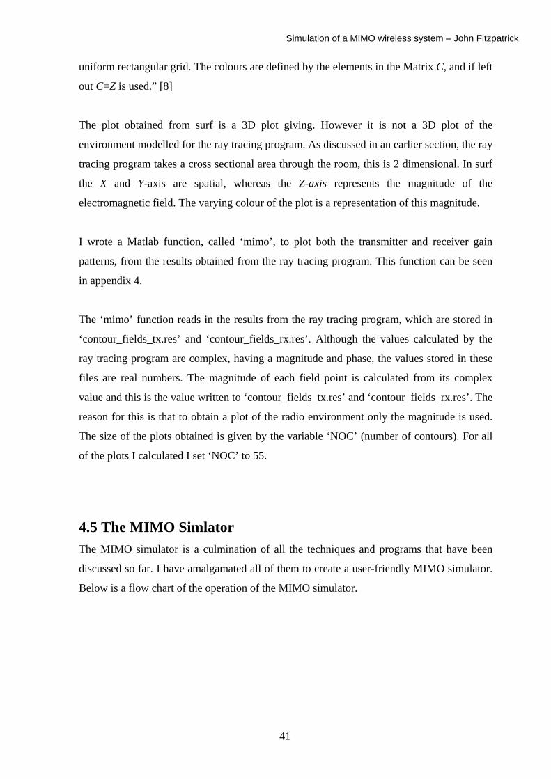
Simulation of a MIMO wireless system – John Fitzpatrick
uniform rectangular grid. The colours are defined by the elements in the Matrix C, and if left
out C=Z is used.” [8]
The plot obtained from surf is a 3D plot giving. However it is not a 3D plot of the
environment modelled for the ray tracing program. As discussed in an earlier section, the ray
tracing program takes a cross sectional area through the room, this is 2 dimensional. In surf
the X and Y-axis are spatial, whereas the Z-axis represents the magnitude of the
electromagnetic field. The varying colour of the plot is a representation of this magnitude.
I wrote a Matlab function, called ‘mimo’, to plot both the transmitter and receiver gain
patterns, from the results obtained from the ray tracing program. This function can be seen
in appendix 4.
The ‘mimo’ function reads in the results from the ray tracing program, which are stored in
‘contour_fields_tx.res’ and ‘contour_fields_rx.res’. Although the values calculated by the
ray tracing program are complex, having a magnitude and phase, the values stored in these
files are real numbers. The magnitude of each field point is calculated from its complex
value and this is the value written to ‘contour_fields_tx.res’ and ‘contour_fields_rx.res’. The
reason for this is that to obtain a plot of the radio environment only the magnitude is used.
The size of the plots obtained is given by the variable ‘NOC’ (number of contours). For all
of the plots I calculated I set ‘NOC’ to 55.
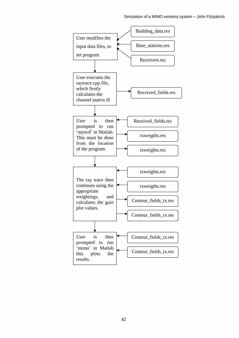
4.5 The MIMO Simlator The MIMO simulator is a culmination of all the techniques and programs that have been
discussed so far. I have amalgamated all of them to create a user-friendly MIMO simulator.
Below is a flow chart of the operation of the MIMO simulator.
41
Simulation of a MIMO wireless system – John Fitzpatrick
Building_data.res
The ray trace then continues using the appropriate weightings, and calculates the gain plot values.
User is then prompted to run ‘mysvd’ in Matlab. This must be done from the location of the program.
User executes the raytrace.cpp file, which firstly calculates the channel matrix H
Received_fields.res
rxweigths.res
txweights.res
txweights.res
rxweigths.res
Contour_fields_tx.res
Contour_fields_rx.res
User modifies the
input data files, to
set program
Base_stations.res
Receivers.res
Received_fields.res
User is then prompted to run ‘mimo’ in Matlab this plots the results.
Contour_fields_rx.res
Contour_fields_tx.res
42
Simulation of a MIMO wireless system – John Fitzpatrick
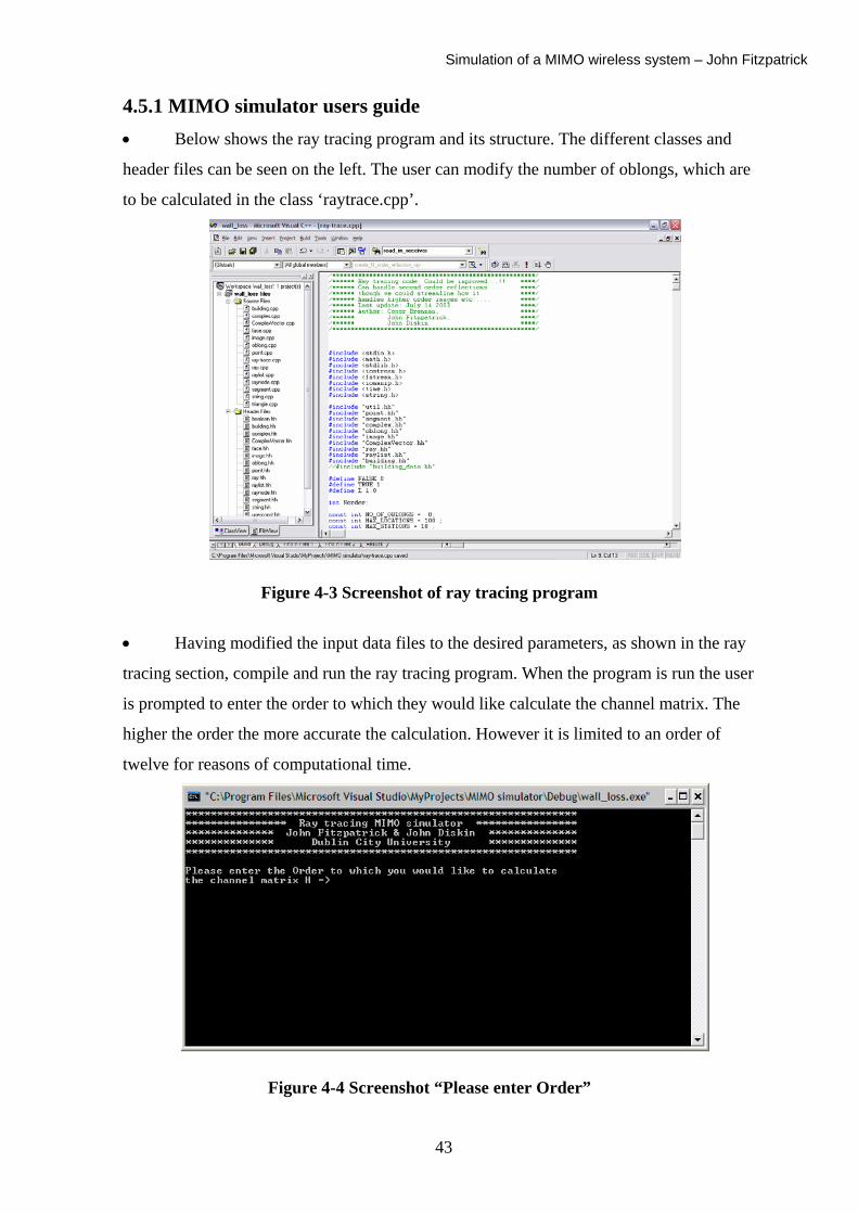
4.5.1 MIMO simulator users guide • Below shows the ray tracing program and its structure. The different classes and
header files can be seen on the left. The user can modify the number of oblongs, which are
to be calculated in the class ‘raytrace.cpp’.
Figure 4-3 Screenshot of ray tracing program
• Having modified the input data files to the desired parameters, as shown in the ray
tracing section, compile and run the ray tracing program. When the program is run the user
is prompted to enter the order to which they would like calculate the channel matrix. The
higher the order the more accurate the calculation. However it is limited to an order of
twelve for reasons of computational time.
Figure 4-4 Screenshot “Please enter Order”
43
Simulation of a MIMO wireless system – John Fitzpatrick
• At this stage the program will calculate the channel matrix H, and the window below
will be displayed. This requests that the user execute ‘mysvd’ in Matlab. This must be done
from the folder in which the program is resident.
Figure 4-5 Screenshot “Please run ‘mysvd’ ”
• When the user runs ‘mysvd’, Matlab creates the weighting files. The user must then
type ‘y’ for the program to continue. The user is then prompted to enter the order to which
they would like to calculate the antenna gain patterns. I recommend an order of 3 to 4, for
reasons of computational time and for reasons of convergence as discussed previously. Once
the program completes the user is presented with the following screen and asked to run the
function ‘mimo’ in Matlab.
Figure 4-6 Screenshot “Please run ‘mimo’“
44
Simulation of a MIMO wireless system – John Fitzpatrick
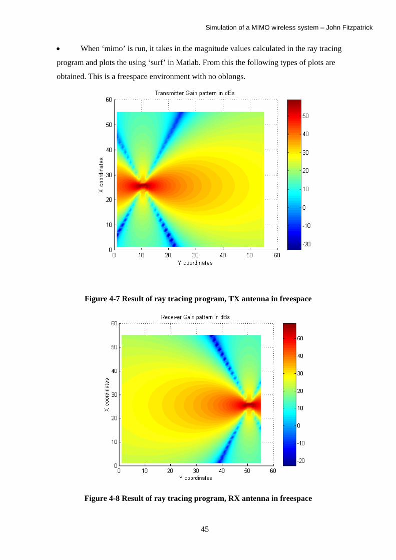
• When ‘mimo’ is run, it takes in the magnitude values calculated in the ray tracing
program and plots the using ‘surf’ in Matlab. From this the following types of plots are
obtained. This is a freespace environment with no oblongs.
Figure 4-7 Result of ray tracing program, TX antenna in freespace
Figure 4-8 Result of ray tracing program, RX antenna in freespace
45
Simulation of a MIMO wireless system – John Fitzpatrick
Chapter 5 – Results
5.1 SVD in Freespace The advantage of the Singular Value Decomposition (SVD), when used in a MIMO system
can best be seen in freespace. The number of channels available in freespace is only one.
This is because in freespace there are no objects to scatter the rays in the environment. The
diagonal matrix for the following freespace system is:
From this it is clear that there
are calculated from the ‘mysv
done the following plots are o
Figure 5-
S =
7.0637 0 0
0 0.0138 0
0 0 0.0000
is essentially only one sub channel available. The weightings
d’ algorithm and applied to the antenna arrays. When this is
btained.
1 TX freespace antenna gain plot
46
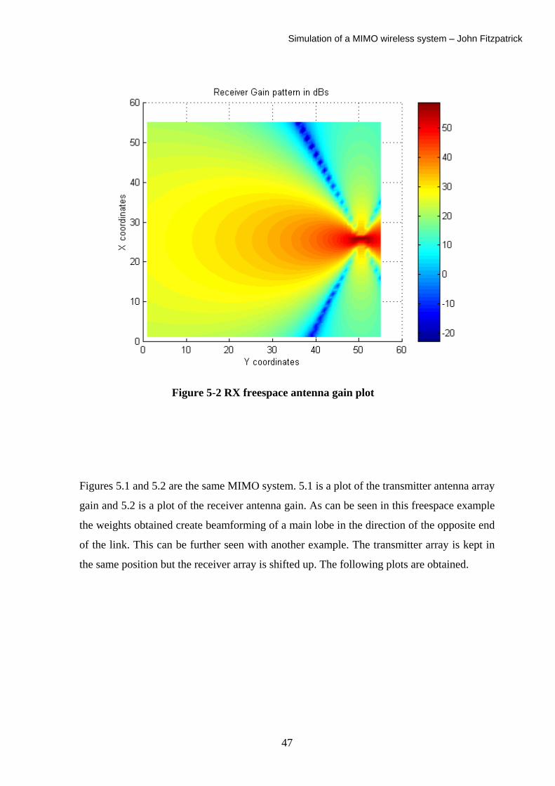
Simulation of a MIMO wireless system – John Fitzpatrick
Figure 5-2 RX freespace antenna gain plot
Figures 5.1 and 5.2 are the same MIMO system. 5.1 is a plot of the transmitter antenna array
gain and 5.2 is a plot of the receiver antenna gain. As can be seen in this freespace example
the weights obtained create beamforming of a main lobe in the direction of the opposite end
of the link. This can be further seen with another example. The transmitter array is kept in
the same position but the receiver array is shifted up. The following plots are obtained.
47
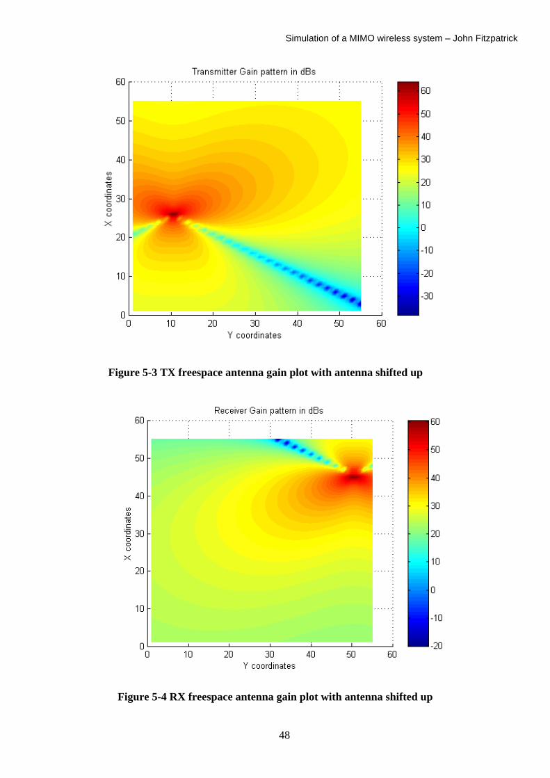
Simulation of a MIMO wireless system – John Fitzpatrick
Figure 5-3 TX freespace antenna gain plot with antenna shifted up
Figure 5-4 RX freespace antenna gain plot with antenna shifted up
48
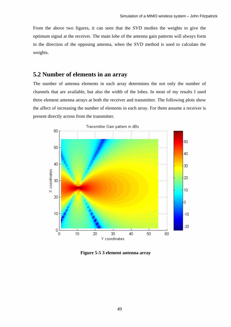
Simulation of a MIMO wireless system – John Fitzpatrick
From the above two figures, it can seen that the SVD modies the weights to give the
optimum signal at the receiver. The main lobe of the antenna gain patterns will always form
in the direction of the opposing antenna, when the SVD method is used to calculate the
weights.
5.2 Number of elements in an array The number of antenna elements in each array determines the not only the number of
channels that are available, but also the width of the lobes. In most of my results I used
three element antenna arrays at both the receiver and transmitter. The following plots show
the affect of increasing the number of elements in each array. For them assume a receiver is
present directly across from the transmitter.
Figure 5-5 3 element antenna array
49
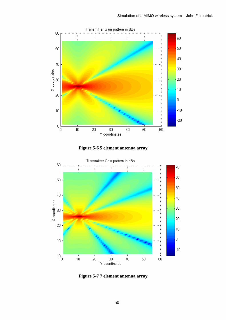
Simulation of a MIMO wireless system – John Fitzpatrick
Figure 5-6 5 element antenna array
Figure 5-7 7 element antenna array
50

Simulation of a MIMO wireless system – John Fitzpatrick
As can be seen from the above figures, as the number of elements in the antenna array
increases the width of the main lobe decreases. This is due to there being more elements
available to create the constructive and destructive interference necessary.
5.3 Dielectric parameters and corridor model The next test I carried out was to look at the effects of different dielectric parameters in the
oblongs, on the radio environment. As discussed earlier each oblong has material parameters
ε (permittivity), µ (permeability), and δ (conductivity). Changing these parameters will
affect the reflectivity of each oblong. Since MIMO relies on the scattering in the
environment, an increase in the reflectivity should give an increase in the quality of each sub
channel.
I essentially combined two experiments into one. One experiment observed the affect of the
different dielectric parameters on the radio environment, and one looked at the change in the
MIMO channels that this increase in reflectivity causes. For the calculation of the channel
matrix each of the antenna elements in the plots have no weighting applied, only the
normalised weight. Hence each antenna element is omni directional. The Singular Value
Decomposition (SVD), on this channel matrix not only gives the weights, but also gives the
relative quality of each sub channel.
With the ε (permittivity), µ (permeability), and δ (conductivity) set to the following
values respectively 3.0, 1.0, and 0.0 for the both oblongs.
51
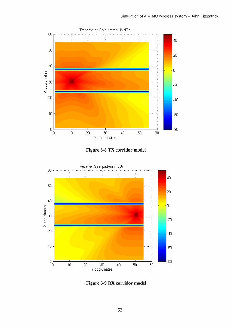
Simulation of a MIMO wireless system – John Fitzpatrick
Figure 5-8 TX corridor model
Figure 5-9 RX corridor model
52
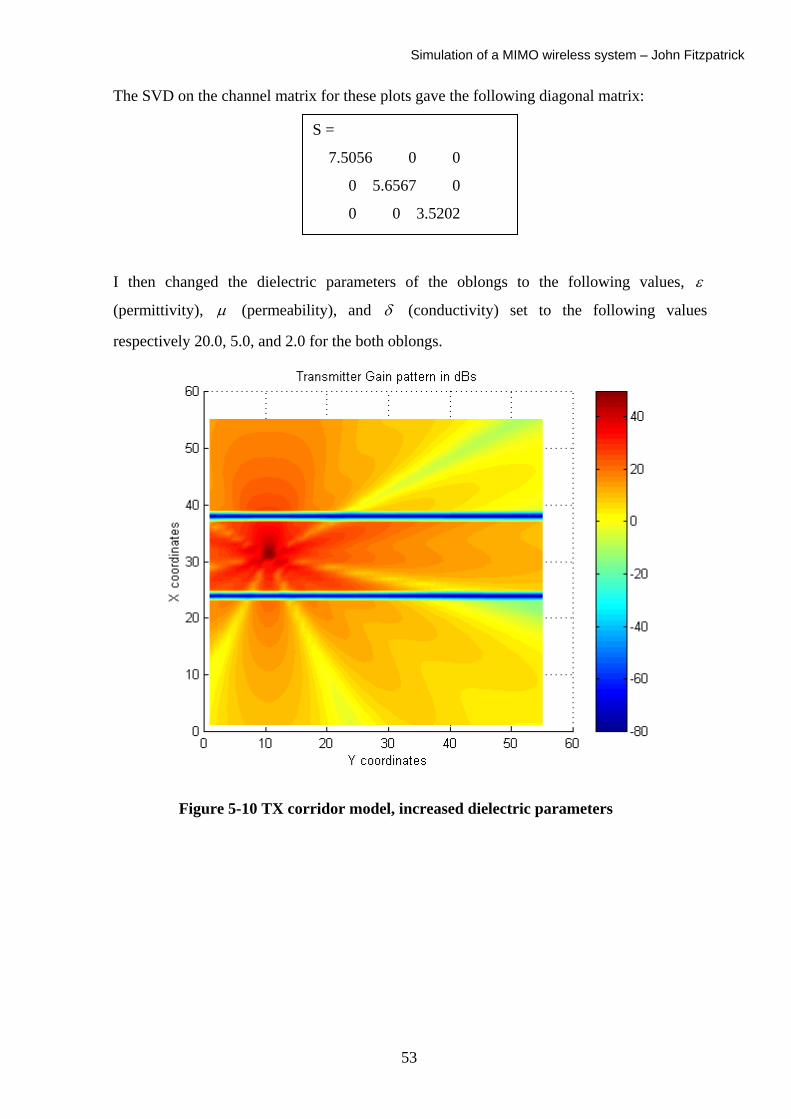
Simulation of a MIMO wireless system – John Fitzpatrick
The SVD on the channel matrix for these plots gave the following diagonal matrix:
I then changed the dielectr
(permittivity), µ (permeabi
respectively 20.0, 5.0, and 2.0
Figure 5-10 TX cor
S =
7.5056 0 0
0 5.6567 0
0 0 3.5202
ic parameters of the oblongs to the following values, ε
lity), and δ (conductivity) set to the following values
for the both oblongs.
ridor model, increased dielectric parameters
53
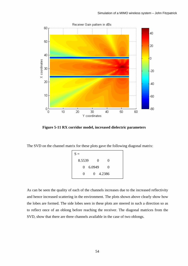
Simulation of a MIMO wireless system – John Fitzpatrick
Figure 5-11 RX corridor model, increased dielectric parameters
The SVD on the channel matrix for these plots gave the following diagonal matrix:
S =
8.5539 0 0
0 6.0949 0
0 0 4.2386
As can be seen the quality of each of the channels increases due to the increased reflectivity
and hence increased scattering in the environment. The plots shown above clearly show how
the lobes are formed. The side lobes seen in these plots are steered in such a direction so as
to reflect once of an oblong before reaching the receiver. The diagonal matrices from the
SVD, show that there are three channels available in the case of two oblongs.
54
Simulation of a MIMO wireless system – John Fitzpatrick
Chapter 6 - Conclusions and Further Research
The original goal of the project goal was to develop a MIMO simulator this was achieved.
The developed program was written in C++ and Matlab. It allows for the simulation of a
MIMO system, operating in an indoor 3D radio environment. The program is user friendly
and very easily modified to model different indoor environments.
Throughout the course of this project I learned a great deal about radio wave propagation
and electromagnetics in general. Up to the point of beginning my project I had very little
experience in C++, and so I was forced to develop my ability in this area, to become
proficient enough to carry out the rather complex C++ aspect of the project. I also further
developed my knowledge of Matlab and numerical techniques. Due to time constraints,
there are some aspects of the simulator that I would have liked to develop further.
The calculation of the Singular Value Decomposition (SVD) is currently performed in
Matlab, and the result files imported into the ray tracing part. I would have liked to complete
the work I started on creating an SVD algorithm in C++. I have a working SVD algorithm
for real numbers only, and I would have liked this to also incorporate complex values. The
advantage of this would be in simplifying the operation for the user. The user would not
have to use Matlab, but rather, all of the calculations would be carried out automatically in
C++.
Currently the MIMO simulator takes a rather simplistic view of the channel model, by
ignoring noise. Further work in improving the simulator might be to create a more realistic
channel model. Noise could be incorporated into the system by not discounting the noise
factor in the system model as I did. The noise factor could be modelled as a vector of
complex Gaussian values with zero mean. The maximum magnitude of the Gaussian
variables could be varied to simulate varying noisy environments.
I would have also liked to explore the by simulation the increases in capacity and bit rates
offered by MIMO systems. This could be compared with traditional Single input Single
Output (SISO) systems, different Multipath environments, and also MIMO systems with
varying numbers of antenna elements.
55

Simulation of a MIMO wireless system – John Fitzpatrick
There was one unusual problem with the MIMO simulator that I only noticed toward the end
of my project. The spacing between each of the antenna elements seems to be crucial. On
some occasions when I ran the simulator I obtained strange plots, however when only the
antenna elements spacing were changed to different values the simulator worked correctly. I
would have like to investigate this problem more to find the cause of the problem. My
advice is to use an antenna spacing of 0.37 times the wavelength.
All of these improvements could be added into the current MIMO simulator to make it more
realistic and more efficient. I thoroughly enjoyed carrying out this project and learnt a great
deal.
56
Simulation of a MIMO wireless system – John Fitzpatrick
References [1] Deprettere, F. (Ed), “SVD and signal processing: Algorithms, Applications and
Architectures”, North Holland, 1988, pp3-43
[2] Durgin, G. “Ray tracing applied to radio wave propagation prediction”,
http://www.taiyang.mprg.ee.vt.edu, 1998, (21-January-2004)
[3] Gesbert, D. et al, “From theory to practice: An overview of MIMO space-time
coded wireless systems”, IEEE Journal On Selected Areas In Communications, Vol.
21, No.3, April 2003
[4] Haardt, M and Spencer, Q, “Smart antennas for wireless communications beyond the
third generation”, Computer Communications, Vol.26, pp41-45, 2003
[5] Holter, B, “On the capacity of the MIMO channel – A tutorial introduction”,
http://www.tele.ntnu.no, 2001, (17-February-2004)
[6] Kreyszig, E., “Advanced Engineering Mathematics”, Wiley, 1988
[7] Litva, J. and Titus Kwok-Yeung Lo, “Digital beamforming in wireless
communications”, Arktech House Publishers, 1996, pp1-55
[8] Part-Enander, E. and Sjoberg, A., “The Matlab hanbook 5”, Prentice Hall, 1999
[9] Porrat, D. “The physics of urban cellular systems: Radio wave propagation along
streets”, http://wireless.stanford.edu/~dporrat/research.html, 2001, (22-March-2004)
[10] Vcelak, J. et al, “Multiple Input Multiple Output wireless systems”, Electrotechnical
Review, 70(4): 234-239, 2003 [11] Ziemelis, J. “Some problems of ray tracing”, http://www.rsf.rtu.lv, 2000,
(15-December-2003)
[12] “Introduction to the Uniform geometrical theory of diffraction”
57
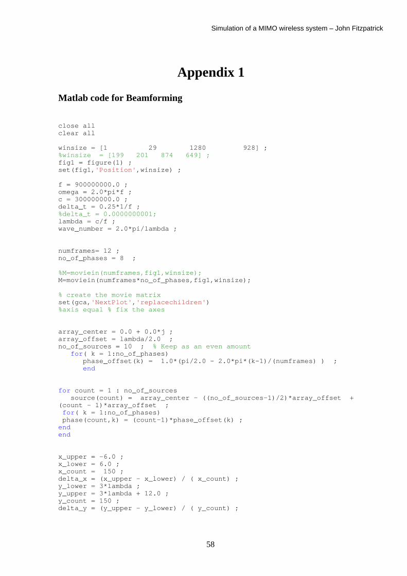
Simulation of a MIMO wireless system – John Fitzpatrick
Appendix 1
Matlab code for Beamforming close all clear all winsize = [1 29 1280 928] ; %winsize = [199 201 874 649] ; fig1 = figure(1) ; set(fig1,'Position',winsize) ; f = 900000000.0 ; omega = 2.0*pi*f ; c = 300000000.0 ; delta_t = 0.25*1/f ; %delta_t = 0.0000000001; lambda = c/f ; wave_number = 2.0*pi/lambda ; numframes= 12 ; no_of_phases = 8 ; %M=moviein(numframes,fig1,winsize); M=moviein(numframes*no_of_phases,fig1,winsize); % create the movie matrix set(gca,'NextPlot','replacechildren') %axis equal % fix the axes array_center = 0.0 + 0.0*j ; array_offset = lambda/2.0 ; no_of_sources = 10 ; % Keep as an even amount for( k = 1:no_of_phases) phase_offset(k) = 1.0*(pi/2.0 - 2.0*pi*(k-1)/(numframes) ) ; end for count = 1 : no_of_sources source(count) = array_center - ((no_of_sources-1)/2)*array_offset + (count - 1)*array_offset ; for( k = 1:no_of_phases) phase(count,k) = (count-1)*phase_offset(k) ; end end x_upper = -6.0 ; x_lower = 6.0 ; x_count = 150 ; delta_x = (x_upper - x_lower) / ( x_count) ; y_lower = 3*lambda ; y_upper = 3*lambda + 12.0 ; y_count = 150 ; delta_y = (y_upper - y_lower) / ( y_count) ;
58
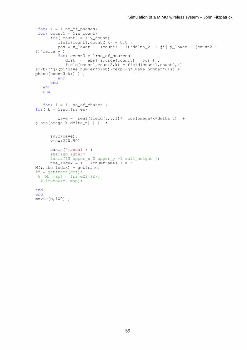
Simulation of a MIMO wireless system – John Fitzpatrick
for( k = 1:no_of_phases) for( count1 = 1:x_count) for( count2 = 1:y_count) field(count1,count2,k) = 0.0 ; pos = x_lower + (count1 - 1)*delta_x + j*( y_lower + (count2 - 1)*delta_y ) ; for( count3 = 1:no_of_sources) dist = abs( source(count3) - pos ) ; field(count1,count2,k) = field(count1,count2,k) + sqrt(2*j/(pi*wave_number*dist))*exp(-j*(wave_number*dist + phase(count3,k)) ) ; end end end end for( l = 1: no_of_phases ) for( k = 1:numframes) wave = real(field(:,:,l)*( cos(omega*k*delta_t) + j*sin(omega*k*delta_t) ) ) ; surf(wave); view(270,90) caxis('manual') ; shading interp %axis([0 upper_x 0 upper_y -1 wall_height ]) the_index = (l-1)*numframes + k ; M(:,the_index) = getframe; %f = getframe(gcf); % [M, map] = frame2im(f); % imshow(M, map); end end movie(M,100) ;
59
Simulation of a MIMO wireless system – John Fitzpatrick
Appendix 2
C++ Gaussian Elimination Code //John Fitzpatrick TC4 DCU
//Gaussian elimination
#include <stdio.h>
#include <math.h>
#include <stdlib.h>
#include <iostream.h>
#include <fstream.h>
#include <iomanip.h>
#include <time.h>
#include <string.h>
#include "complex.hh"
const int N = 2; //Number of rows and columns (Square matrix)
void gauss(complex **tempmat) //Function reads in temporary
matrix
{
int i, j;
complex a[N][N+1]; //Matrix which will be used
//********Converts from temp pointed array to 2D array
for(i=0; i<N; i++)
{
for(j=0; j<=N; j++)
{
a[i][j]=tempmat[i][j];
}
}
//*****************************************************
60
Simulation of a MIMO wireless system – John Fitzpatrick
//*****Takes in the received signal vector from user
float real, imag;
cout << "Enter in the received signal vector" << endl;
for(i=0; i<N; i++)
{
cout <<"r" << i << " real : ";
cin >> real;
cout <<"r" << i << " imag : ";
cin >> imag;
a[i][N]=complex(real, imag);
}
//******************************************************
complex s[N];
//********Print out of Augmented Matrix A^
cout << "The Augmented matrix is:"<< endl;
for(i=0; i < N; i++)
for(j=0; j<N+1; j++)
cout<< a[i][j] <<endl;
//************************************************
//******perform elimination step
for(int index=0; index<=N; index++)
{
complex pivot;
for(int row=index+1; row<=N-1; row++)
{
pivot = -a[row][index]/a[index][index];
for(int column=index+1; column<=N; column++)
{
a[row][column]=a[index][column]*pivot+a[row][column];
61
Simulation of a MIMO wireless system – John Fitzpatrick
}
}
//**************************************************
//*********perform back substitution step.
s[N-1]=a[N-1][N]/a[N-1][N-1];
for (row=N; row>=0; row--)
{
for(int column=N-1; column>=row+1; column--)
{
a[row][N]=s[column]*a[row][column]-
a[row][N];
}
s[row]= a[row][N]/a[row][row];
}
//**********************************************
}
//*****************Print answer
cout<< "The transmitted signal vector is " << endl;
for(i=0; i<=N-1; i++)
{
cout << s[i]<< endl;
}
//**********************************
}
void main()
{
int i;
complex b[N][N+1], **bb;
62

Simulation of a MIMO wireless system – John Fitzpatrick
b[0][0]=complex(-1.265,0.8963);
b[0][1]=complex(1.109,0.1234);
b[1][0]=complex(0.567,-1.64);
b[1][1]=complex(1.892,0.2454);
//*****Needed to convert 2D array to pointed array
bb=(complex **) malloc((unsigned) N*sizeof(complex*));
for(i=0;i<=N-1;i++) bb[i]=b[i];
//****************************************************
gauss(bb);
}
63
Simulation of a MIMO wireless system – John Fitzpatrick
Appendix 3
Matlab Singular Value Decomposition (SVD) Code %Reads in complex matrix in tabbed format from a '*.res' file %Computes SVD of a complex channel matrix %Finds wieghtings to be applied to receive and %transmit antennas for MIMO systems and writes result to '*.res files' %*********************************************************************** [re, im]=textread('received_fields.res','%f %f'); %Loads in real and imag parts of txt file htemp=complex(re, im); %Creates N^2 size vector of channel matrix values size(htemp); N=ans(1); %Finds size of matrix N index=1; %Converts htemp Vector to H channel Matrix q=1; for R = 1:(sqrt(N)), for C = 1:(sqrt(N)), H(R,C)=htemp(index); if q<=N, index=index+1; end end end %*********************************************************************** [U,S,V] = svd(H); for l = 1:(sqrt(N)), s(l)=complex(1.0,0); %Creates the normailised transmit weighting vector s end txweights=s*S*(V')%Calculates the transmitter weightings rxweights=s*(U') %Calculates the receiver weightings %*******************Write tx weights to file**************************** for R = 1:(sqrt(N)), realtemp(R)=real(txweights(R)); imagtemp(R)=imag(txweights(R)); end for R = 1:(sqrt(N)), txtemp(R,1)=realtemp(R); txtemp(R,2)=imagtemp(R); end txfile = fopen('transmitweight.res','w'); for R = 1:(sqrt(N)), fprintf(txfile,'%f\t',realtemp(R)); fprintf(txfile,'%f\n',imagtemp(R)); end fclose(txfile); %*******************Write rx weights to file**************************** for R = 1:(sqrt(N)), realtemp(R)=real(rxweights(R)); imagtemp(R)=imag(rxweights(R)); end
64
Simulation of a MIMO wireless system – John Fitzpatrick
for R = 1:(sqrt(N)), rxtemp(R,1)=realtemp(R); rxtemp(R,2)=imagtemp(R); end rxfile = fopen('receiveweight.res','w'); for R = -(sqrt(N)):-1, G=-R; fprintf(rxfile,'%f\t',realtemp(G)); fprintf(rxfile,'%f\n',imagtemp(G)); end fclose(rxfile);
65
Simulation of a MIMO wireless system – John Fitzpatrick
Appendix 4
Matlab ‘mimo’ Code load 'contour_fields_tx.res' NOC = 55 ; fields = zeros(NOC,NOC) ; for( count1 = 1:NOC) for( count2 = 1:NOC) fields(count1, count2) = contour_fields_tx((count1 - 1)*NOC + count2 ) ; end end figure(1); surf(fields,'FaceColor','red','EdgeColor','none'); lighting phong view(0,90) shading interp colorbar title 'Transmitter Gain pattern in dBs' xlabel('Y coordinates') ylabel('X coordinates') load 'contour_fields_rx.res' NOC = 55 ; fields = zeros(NOC,NOC) ; for( count1 = 1:NOC) for( count2 = 1:NOC) fields(count1, count2) = contour_fields_rx((count1 - 1)*NOC + count2 ) ; end end figure(2); surf(fields,'FaceColor','red','EdgeColor','none'); lighting phong view(0,90) shading interp colorbar title 'Receiver Gain pattern in dBs' xlabel('Y coordinates') ylabel('X coordinates')
66