Simulation and Experimental Study

of SCM/WDM Optical Systems

Renxiang Huang

B.S.E.E., Beijing University of Posts & Telecommunications, 1993

Submitted to the Department of Electrical Engineering and ComputerScience and the Faculty of the Graduate School of the University ofKansas in partial fulfillment of the requirements for the degree ofMaster of Science

Thesis Committee:

Chairman

Date of Defense: May 23, 2001

i

Abstract

High-speed data transmission utilizing optical subcarrier multiplexing (SCM)

techniques was recently studied by experiments and simulations in several works

[1,2,3,4]. SCM may have better spectral efficiency than WDM and SCM system

could be less subjected to fiber dispersion than TDM system because the data rate at

each subcarrier is low. These works used amplitude shift keying (ASK) as the RF

modulation format and used double side band (DSB) as the optical modulation

method, they used optical filter to select each subcarrier channel and detect the ASK

signal directly. The reported transmission distances were about 500km.

In our study, optical-single-side-band modulation (OSSB) was used since it

further increases the spectrum efficiency and significantly decreases the dispersion

penalty; Multiple phase shift keying (MPSK) RF modulation was used due to its high

spectral efficiency and simple demodulation. We have developed a simulation model

and simulated 3 types of SCM systems --- 4-subcarrier binary phase shift keying

(BPSK) system, 2-subcarrier quadrant phase shift keying (QPSK) system, 4-

subcarrier ASK system. We also show the result of a standard IMDD WDM system

for comparison. These 4 types of systems all use 4 wavelengths with 50GHz spacing

and have same total capacity (40Gbps). We did an experiment of a single wavelength

4 channel BPSK SCM system (total 10 Gbps capacity) over 75 km standard single

mode fiber.

There are two major limiting factors for the system performance, namely

nonlinear distortion and accumulated ASE noise. For SCM systems, the nonlinear

interference between subcarrier channels is severe because the channel spacing is

very narrow and the interference components fall into the signal frequencies. In order

to limit nonlinear interference, the signal optical power can not be too high. On the

other hand, in order to keep an acceptable signal-to-noise ratio (SNR) in the presence

of accumulated ASE noise, the optical power can not be too small. Therefore

parameter optimization is essential in the system design. A major benefit of SCM

systems is their immunity to fiber dispersion. This type of systems and hence they is

ii

suitable to be used in those situations which require high spectrum efficiency and do

not have dispersion compensation.

Polarization walkoff and PMD effects were assessed preliminarily in this

work and further simulation and experiments are suggested to determine their exact

impact on the system performance.

Our simulation results revealed that with dispersion compensations, the

longest transmission distance for BPSK system is 450 km, QPSK system is 1200km,

ASK SCM system is 250km, IMDD system is 1100km. If there is no dispersion

compensation, these numbers are 250 km, 450 km, 550 km and 100 km respectively.

Acknowledgements

I would like to express my deepest gratitude to my advisor and mentor, Dr.

Rongqing Hui, for his invaluable guidance and unwavering support throughout my

education at the University of Kansas. Without his encouragement and patience, this

work can not be done. I would also like to extent my gratitude to Dr. Kenneth

Demarest and Dr. Christopher Allen for serving on my thesis committee and their

encouragement.

I would like to thank Dr. Benyuan Zhu and Chris Johnson for valuable

discussions on the SCM experiment. I also thank Dr. Kumar (Vijay)

Peddanarappagari for those enlightening discussions on simulation methods.

A special thanks to Yonggang Wang for his numerous help and

encouragement. My gratitude also goes to other members of the Lightwave Group, in

particular, Hok-Yong Pua and Dan Tebben for their friendly help and caring.

Finally, I want to express my gratitude and love to my wife, Ying Tian.

Without her loving support and encouragement, I would not have accomplished this

goal.

Table of Contents

CHAPTER ONE BACKGROUND AND INTRODUCTION...............................1

1.1 INTRODUCTION AND MOTIVATION ...........................................................11.2 SCM AS A VIABLE SOLUTION.......................................................................21.3 ORGANIZATION OF THE THESIS..................................................................9

CHAPTER TWO NUMERICAL MODEL FOR THE SCM SYSTEM ............10

2.1 GENERAL CONSIDERATIONS FOR NUMERICAL SIMULATION OFOPTICAL SCM FIBER TRANSMISSION SYSTEMS .........................................102.2 BASIC INFORMATION OF THE NUMERICAL MODEL OF OPTICALSCM SYSTEMS ......................................................................................................122.3 TRANSMITTER SIDE SIMULATION MODELS ..........................................13

2.3.1 Baseband signal generation ........................................................................152.3.2 Subcarrier signal generation.......................................................................172.3.3 Mach-Zehnder modulator............................................................................21

2.3.3.1 Principle of MZ modulator....................................................................212.3.3.2 The realization of single side band optical modulation.........................222.3.3.3 Nonlinear distortion of unlinearized modulator ....................................26

2.3.4 Carrier suppression.....................................................................................302.3.5 Transmitter optical filter .............................................................................352.3.6 The post optical amplifier............................................................................36

2.4 OPTICAL FIBER PATH..................................................................................382.4.1 Nonlinear Schrodinger Equations ...............................................................392.4.2 Numerical solution ......................................................................................40

2.5 SCM RECEIVER...............................................................................................432.5.1 Optical demux..............................................................................................432.5.2 Preamplifier.................................................................................................442.5.3 Photodiode...................................................................................................442.5.4 High pass filter ............................................................................................452.5.5 Microwave coupler ......................................................................................452.5.6 Carrier recovery ..........................................................................................452.5.7 Demodulation ..............................................................................................492.5.8 Electrical filters ...........................................................................................502.5.9 Bit Synchronization procedure ....................................................................522.5.10 Polarization effects in SCM system ...........................................................52

2.5.10.1 Polarization walkoff ............................................................................522.5.10.2 Polarization mode dispersion ..............................................................53

2.5.11 Analytical estimation of the Error probability (Bit-Error-Rate) ..............552.5.12 Calculation of Receiver sensitivity ............................................................57

2.5.12.1 Noise from optical amplifier ...............................................................572.5.12.2 Sensitivity estimation for a digital BPSK SCM system......................59

2.5.12.3 Sensitivity Evaluation for QPSK SCM system ...................................622.5.12.4 Sensitivity Evaluation for a binary ASK system.................................62

CHAPTER THREE SIMULATION RESULTS OF SCM SYSTEMS..............64

3.1 PERFORMANCE OF AN SCM SYSTEM USING 4 BPSK SUBCARRIEREACH WITH OC48 DATA, AND WITH SELF-COHERENT DETECTION ......65

3.1.1 Bandwidth of the electrical filters ...............................................................653.1.2 Channel spacing ..........................................................................................673.1.3 Frequency plan ............................................................................................683.1.4 Effect of Carrier Suppression ......................................................................723.1.5 OMI and carrier suppression ratio combination ........................................733.1.6 Simulation results of System sensitivity and eye-opening............................77

3.2 PERFORMANCE OF AN SCM SYSTEM USING QPSK ..............................813.3 PERFORMANCE OF AN SCM SYSTEM WITH DIRECT DETECTION.....88

3.3.1 The impact of FP filter bandwidth...............................................................983.3.2 Optical modulation index and the suppression ratio...................................993.3.3 Effect of optical power...............................................................................1013.3.4 Four wavelength system results.................................................................102

3.4 SYSTEM PERFORMANCE FOR A TRADITIONAL FOUR WAVELENGTHOC192 SYSTEM ...................................................................................................103

CHAPTER FOUR BPSK SCM SYSTEM EXPERIMENTS............................104

4.1 BER TEST .......................................................................................................1084.2 CHANNEL SPACING ....................................................................................1104.3 CARRIER SUPPRESSION .............................................................................1114.4 COMPARISON BETWEEN SCM AND TDM AT OC192 RATES:.............113

CHAPTER FIVE CONCLUSION AND FUTURE WORK..............................115

Future work ........................................................................................................117

REFERENCES…………………………………………………………………….118

APPENDIX 1 SOME CONSIDERATIONS FOR THE SIMULATION OF COMMUNICATIONS SYSTEMAPPENDIX 2 BPSK SCM RESULTSAPPENDIX 3 QPSK SCM RESULTSAPPENDIX 4 ASK SCM RESULTSAPPENDIX 5 OC192 RESULTS

1

Chapter One

Background and Introduction

1.1 Introduction and Motivation

The prevalent utilization of Internet by business and consumer has been generating

a global demand for huge bandwidth. In recent years, as new bandwidth hungry

applications like internet video and audio and new access technologies such as xDSL

become more popular, optical communications networks are finally feeling the

bandwidth constraints already faced in many other communications networks such as

wireless and satellite communication systems. Service providers are searching for

ways to increase their fiber optic network capacity.

In order to solve this problem, people have been trying to make full use of the huge

bandwidth provided by optical fibers. Technologies like TDM, WDM and their

combinations are used and improved.

The TDM strategy is to increase the bit rate carried by a single optical

wavelength. These systems use very short pulses to achieve very high bit rate and

thus they are subject to the influence of dispersion (because of the wide bandwidth of

the signal) and nonlinearities (because of the required high power to overcome the

noise). High speed TDM systems are very sensitive to the PMD effect and they are

also limited by the achievable speed of electronic components and devices. Because

of those constraints, the data rate of commercial optical fiber systems is currently

limited at 10Gb/s. For some old fiber plants, the maximum per-channel data rate is

2.5Gb/s due to the limitation in their poor PMD characteristic.

Later, as technology advanced, WDM came along. The WDM strategy is to make

better use of optical fiber bandwidth by stacking many TDM channels into the same

fiber. The advantage of WDM over TDM is that WDM usually use much lower bit

rates and optical power in each channel while achieving a higher total capacity.

Hence, the issues in high-speed TDM such as PMD, chromatic dispersion, fiber

2

nonlinearities become mitigated. However, there are many factors that limit the

system performance of WDM. The wavelength stability of semiconductor lasers and

selectivity of optical filters limit the minimum channel spacing from 50GHz to

100GHz in current commercial WDM systems. As an example, for a WDM system of

2.5Gb/s per-channel data rate and 50GHz channel spacing, the bandwidth efficiency

is only 0.05 bit/Hz. How to further increase the efficiency of bandwidth utilization

while maintaining quality transmission? This problem still remains as a challenge to

the optical communication society.

1.2 SCM as a viable solution

One technology that can be used to increase the efficiency of bandwidth utilization

is the Sub-carrier multiplexing (SCM). It is an old technology that has been studied

and applied extensively in microwave and wireless communication systems. In

optical domain, the most popular SCM application is the optical analog video

transmission and distribution.

SCM technology essentially uses a two step modulation. First, several low

bandwidth RF channels carrying analog or digital signal are combined together and

they are very close to each other in the frequency domain. Then this composite signal

is further modulated onto a higher frequency microwave carrier or optical carrier and

can be transmitted through different media.

Because of its simple and low-cost implementation, high-speed optical data

transmission using SCM technology attracted the attention of many researchers. The

most significant advantage of SCM in optical communications is its ability to place

different optical carriers together closely. This is because microwave and RF devices

are much more mature than optical devices: the stability of a microwave oscillator is

much better than an optical oscillator (laser diode) and the frequency selectivity of a

microwave filter is much better than an optical filter. Therefore, the efficiency of

bandwidth utilization of SCM is expected to be much better than conventional optical

WDM.

3

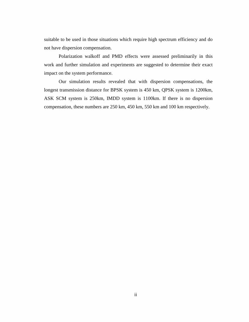
First, let us look at the spectrum of optical digital SCM signal and then later we

will show an example realization of an optical digital SCM system.

fOf3- f2- f1- f4+f3+f2+f1+f4-

a. Optical DSB SCM

b. Optical SSB SCM

fO f4+f3+f2+f1+

optical detectionusing filter

Figure 1.1, Illustration of the spectrums of DSB SCM and SSB SCM signals

Figure 1.1(a) shows the spectrum of traditional SCM system which is double side

band modulated (DSB), it is usually generated by direct modulation of a

semiconductor laser or an external optical modulator like a Mach Zender modulator.

Mach Zender modulator is generally nonlinear in nature. As many different ways to

linearize the Mach Zender modulator are found and available [10], more and more

systems are using MZ modulator to generate the signal. In the figure, ±if is the

frequency of the sub carriers i . Signals are on both sides of the carrier, the total

optical bandwidth is about twice of the bandwidth of the microwave signal or the

modulating signal.

When the bandwidth of the information becomes higher, such as more than several

GHz, and the transmission distance is very long, such as more than hundreds of

kilometers, the DSB scheme will not work if it still use only a simple photon detector

4

to detect. This is because the dispersion of the fiber will give quite different delay to

+if and −if due to the large frequency difference between them. If the relative delay

between +if and −if is comparable to the duration of a baseband bit, then after

photon detector, the two side bands will interfere with each other destructively.

Two methods can be used to solve this problem, one way is to use narrow band

optical filter to filter out each subcarrier channel and then detect them separately. This

is the method used in previous study of high-speed data transmission utilizing SCM

techniques [1,2]. In those studies, DSB is used as the optical modulation method and

ASK is used as the RF modulation format. The demodulation of subcarrier is to filter

out each subcarrier optically in order to avoid the fiber dispersion effect on the double

side band modulation format. ASK RF modulation is used because it makes direct

detection possible. The optical spectrums of these systems are very similar to the

spectrum showing in Figure 1.1 (a).

Another way is to use optical single side band modulation. Figure 1.1 (b) is the

spectrum of optical single side band (OSSB) SCM, the lower side band in the DSB

spectrum is removed by ways such as optical filter or special modulating methods.

The carrier itself could be remove or kept depending on the preferred demodulating

method. The occupied spectrum is only half that of the optical DSB signal.

When optical SSB modulation is used, it will occupy the same bandwidth as the

traditional WDM system if they have the same information bit rate. Figure 1.2 (b) is

showing the spectrum of a traditional WDM system, Figure 1.2 (a) is the spectrum of

a comparable WDM/SCM. Each of the WDM wavelengths carries a SCM composite

signal. In this illustration, the signal bandwidths of the two systems are similar if the

guard band between two adjacent subcarriers is small enough and can be ignored.

In this example, the bit rate of each subcarrier is only one fourth of the

corresponding traditional WDM channel bit rate. 4 subcarriers will give the same

capacity as the traditional WDM. They also occupy the same amount of bandwidth.

5

b. WDM

a. WDM/SCM

f4+f3+f2+f1+

1λ 2λ

1λ 2λ

Figure 1.2, Illustration of the spectrums of WDM/SCM and traditional WDM

Because the dispersion effect is proportional to the square of the bit rate in a TDM

channel of a WDM system, and the dispersion effect on is 16 times more severe in the

traditional WDM system than in the WDM/SCM system, you should be able to

transmit the signal longer in WDM/SCM system than in traditional WDM.

In practice, without SCM technology it is not realistic to place two wavelength

channels at 5GHz spacing in a WDM system due to wavelength stability of laser

diodes and frequency selectivity of optical filters. However, this narrow channel

spacing is possible with sub-carrier multiplexing thanks to the maturity of microwave

technology. Essentially, WDM/SCM is equivalent to packing more WDM channels in

a given optical bandwidth and breaking through the limitations of minimum channel

spacing imposed by current optical device technology.

One additional advantage of SCM is that subcarriers can be modulated using

various formats including phase modulations because RF carriers have stable phase. It

thus can be used in a lot of different network setups and it is easy to be used with

6

traditional Synchronous Optical Network (SONET) equipment. Also because the bit

rate granularity is smaller which facilitates channel add/drop, the combination of

WDM and SCM can potentially make optical networks more flexible.

However SCM technology is subject to some important system penalties. Because

the channel spacing between subcarrier is so small, you will suffer higher nonlinear

distortion. For example, in the lightwave analog video transmission and distribution

[11,12], because the analog signal is very sensitive to any type of distortion such as

device noise and the inter-modulation distortion (composite second-order (CSO)

distortion and composite triple beat (CTO)) due to the nonlinearity of the devices and

the fiber, the system has very stringent requirements on the noise and the linearity of

the system. In digital sub-carrier multiplexing system, even the linearity of the system

and SNR or CNR requirement is not that strict as in analog applications, the major

concerns is still the inter-modulation crosstalk due to the devices and fiber.

Little research has been done for a digital SCM system with optical single side

band and PSK RF modulation. No systematic comparison between a digital SCM

system and a digital binary system has been done. This work will first focus on two

types of SCM systems with OSSB and PSK RF modulation and their performance

with standard G.652 fiber. In one of the systems, there are 4 wavelength and each

wavelength has 4 BPSK subcarriers. Each subcarrier carries OC48 data. In another

one, there are 4 wavelength and each wavelength has 2 QPSK subcarriers. Each

subcarrier carries 2 OC48 data channels. Then we compared these two systems with a

ASK modulated SCM system and a traditional OC192 ASK system.

The motivation to use OSSB and PSK RF modulation is that OSSB can reduce the

bandwidth of the signal and increase the spectrum efficiency. Because OSSB will

reduce the damage of the chromatic dispersion without optical filtering of each

subcarriers, the signal of one wavelength can be converted to electrical signal directly

and then demodulate each subcarrier in the microwave domain.

PSK RF modulation is used because BPSK will have 6dB sensitivity gain against

ASK. We also used QPSK in our system because it has higher spectrum efficiency.

7

We didn’t consider QAM because in [13], the result of the comparison of QAM and

PSK shows that PSK is robust to the nonlinearity of an MZ modulator compared to

16 QAM and 64 QAM, and also the QAM scheme require much higher modulating

signal amplitude to reach the same symbol error rate as the PSK. This is because the

QAM format needs less bandwidth but higher amplitude.

Simulation is the main way of investigation due to its economical advantage.

Experiment was also done for a 1 wavelength 4 subcarriers BPSK SCM system and

comparison between this system and a one wavelength ASK OC192 system is also

done experimentally.

Figure 1.3 is a demonstrating setup of SCM system, at the left side is the

transmitter, in the transmitter, you have m separate optical transmitters, each optical

transmitter use n microwave mixer to generate n subcarriers and combine them as a

composite signal. Then the composite signal is used to modulate the lightwave.

Figure 1.3, A basic configuration of an SCM/WDM optical system

λm

λ1

f1

Σ

f2ch.2

fn

ch.n

.

.

Receiver

ch.1

Opt

ical

WD

M M

UX

Opt

ical

WD

M D

MU

XAdd/drop

f1

Σ

f2

ch.2

fn

ch.n

.

.

Receiver

ch.1

Transmitterf1

Σ

f2

ch.2

fn

ch.n

.

.

λ1ch.1

Transmitterf1

Σ

f2ch.2

fn

ch.n

.

.

λm

ch.1

8

Then the m wavelength channels are combined by an optical WDM multiplexer.

At the receiver, an optical WDM demultiplexer is used to separate different

wavelength, a separated optical detector is used the convert the optical signal into

electrical current, then the electrical signal is sent to n branches. In each branch, the

signal is demodulated by a microwave mixer coherently.

Figure 1.4, Illustration of wavelength arrangement of an SCM/WDM system.

Figure 1.4 is an illustration of wavelength arrangement of an SCM/WDM system

when the n=4 and m=4, the subcarrier channel spacing is 5GHz, the wavelength

spacing is 50GHz,

It is worth mentioning that here we if an optical carrier is transmitted along with

the subcarrier channels then the optical carrier and the subcarrier channels can beat

with each other in the photon diode and generate the microwave signal. In this way,

you don’t have to have a local oscillator like traditional coherent system.

In order to multiplex several sub-carrier digital channels on one wavelength,

wideband microwave devices and wideband electro-optic modulators are necessary.

Currently, commercially available devices have bandwidths around 20GHz to

30GHz. With a 20GHz modulator bandwidth, 4 SCM channels each carrying OC-48

traffic can be accommodated. In this work, the largest number of SCM channels is 4

because it is limited by the device of the lab and also it is an adequate choice for real

applications.

50GHz

λ λ λ λ

5GHz

9

Also, it is not showing in the diagram, since several digital channels are closely

packed on one wavelength, we have to use microwave filters both at the transmitter

and at the receiver to select the desired channel, and these filters must have good

frequency selectivity in order to minimize linear inter-channel crosstalks.

From an optical transmission point of view, as the channel space is much smaller

than traditional WDM system, the fiber nonlinearity will generate much higher

nonlinear interference. Also because the subcarriers are modulated in one optical

wavelength, the nonlinearity of the modulator and the photon detector will also

generate inter channel interference too.

1.3 Organization of the thesis

This thesis is organized into 5 chapters. In chapter 2, the simulation model will be

presented and the issues involved will be explained in details. These issues include

general simulation method; simulation implementation of the modulations, optical

fiber, demodulation; noise calculation; polarization walkoff and PMD issues. In

chapter 3, the simulation results of 3 different types of SCM systems: 4 wavelength 4

BPSK subcarriers SCM, 4 wavelength 2 QPSK subcarrier SCM, 4 wavelength 4 ASK

subcarriers SCM, will be given and the selection of system parameters are examined.

Then a traditional 4 wavelength OC192 WDM system is simulated and the results are

compared to those of SCM systems. In chapter 4, a one wavelength 4 BPSK

subcarriers system is studied experimentally and it is compared with a one

wavelength OC192 system.

And finally, in chapter 5, the thesis is concluded and the problems that need further

studies are discussed and prospected.

10

Chapter Two

Numerical model for the SCM systemIn order to study the feasibility and performance of the SCM system, both

simulation and experiment methods could be used. Due to its economic advantage,

simulation method is used very often in studying communication systems.

First of all, simulation does not require any physical devices and equipment.

Once the simulation model is built, it is very easy to change the system parameters

and the time needed to check a specific setup is usually much smaller comparing to

an experimental investigation. Second, in a simulation, the only limitation is the

computing power of the computer such as CPU speed and memory size. You can

perform a simulation for a complex system while it is very difficult to fulfil in a real

experiment, which requires many devices and equipment.

We used both experimental method and numerical modeling method in our

investigation of the SCM systems. Since the setup of a multi-wavelength SCM

system will require many microwave and optical devices which will cost a lot of

money. We only did an experiment of one wavelength SCM system. Then we

simulate the performance of several different 4-wavelength SCM systems. We will

first present the simulation part in the following two chapters. Then in the fourth

chapter, we will present the experimental result.

In order to understand the setup of the simulated SCM systems and the detail

of the simulation models of the transmitter, optical fiber, receiver etc., in this chapter,

we will introduce the simulation models and discuss some problems that are special

to the SCM simulation.

2.1 General Considerations for numerical simulation of optical SCM

fiber transmission systems

A numerical modeling or simulation program for a system should include the

models of all the components that constitute that specific system. As a system level

11

simulation, the model for each individual component should be kept as simple as

possible when the accuracy requirements allow. It is not necessary to use their

detailed models because it will not significantly increase the overall accuracy of the

simulation but it would increase complexity dramatically and results in a much lower

efficiency. So most of the components in our simulation are assumed to be ideal and

doesn’t behavior exactly like their physical counterpart. But the effect of this

inaccuracy can be ignored because it is very small compare to the distortion of the

fiber and will not have big impact on the final result.

Modeling of the optical fiber system is quite different than the modeling of

other types of communication systems, such as wireless system, due to its high bit

rate, low bit error rate and its transmission media, which needs special consideration.

High bit rate means that the simulation bandwidth has to be very large and the

number of bits you can simulate at one time will have to be small due to the limitation

of the computing hardware. Low bit error rate means a BER lower than 910− and you

have to run a very long simulation in order to see even a single error bit transmitted.

So we use a method called semi-analytical method to calculate the BER of the

system. This method will calculate the noise analytically instead of numerically.

Among all the devices and subsystems of an optical transmission system, the

optical fiber is usually the main source of the system penalty and its modeling is the

most important part of the whole model.

In some situations, analytical calculation can also be used to model the fiber

transmission. Because there is no close form solution to the nonlinear transmission

equation that guard the waveform evolution along the fiber, linear addition model is

applied to the evaluation procedure, every nonlinear effect and the fiber dispersion is

considered separately and then all the effects are added together to get the total

system performance. The interactions between all these effects are ignored.

Compared to analytical methods, the numerical integration of the propagation

equation is generally more accurate and it takes into account all the linear and

12

nonlinear effects automatically. It became quite popular for the performance

evaluation of optical transmission systems.

There are generally two categories of numerical methods which can be used to

solve the equation, one of them is the finite difference method and the other is the

Pseudo-spectral methods, and pseudo-spectral methods is faster by up to an order of

magnitude to achieve the same accuracy. Among the second category, split step

Fourier method is used most extensively to solve the pulse propagation problem in

nonlinear dispersive media. Its fast speed mainly can be attributed to the use of the

fast Fourier transform algorithm. Because its fast speed and easy implementation, we

will use the split step Fourier method as the algorithm for the fiber model.

Most previous simulations on fiber systems use single step modulation and

demodulation, which is commonly referred to as E/O and O/E conversions. The most

often used format is on/off keying modulation. SCM system needs two steps of

modulation and demodulation. The first step modulation is the modulation of

baseband signal into microwave subcarriers and the second step is the E/O

conversion. Demodulation is the reverse of these two steps. Also, SCM can use PSK,

QSK and ASK modulation format. We will simulate the first modulation step in the

real signal domain and the second modulation in the complex signal domain.

In the remaining of this chapter we will explain the detail of our simulation

model.

2.2 Basic information of the numerical model of optical SCM

systems:

We have developed a simulation model in MATLAB because it is flexible and

has many built-in functions like FFT calculation and array manipulation. This model

is capable to simulate a multi-wavelengths sub-carrier multiplexed WDM

transmission system. It can use ASK, BPSK and QPSK as the RF modulation format.

It simulates a dual-electrod Mach-Zender optical modulator and generates optical

DSB or SSB signals. It uses split step Fourier method to simulate the fiber

13

transmission and it considers the impact of fiber dispersion effect and fiber nonlinear

effects such as FWM, XPM, SPM. It calculates the distortion created at various parts

of the system, such as modulation, transmission, and demodulation with numerical

simulation. An analytic method is used to evaluate the effect of noise. The system

performance is evaluated by eye opening and receiver sensitivity.

The simulation model has a graphical user interface and most of the system

parameters can be changed through this interface. It also supports a batch mode and

the user can change the parameters by editing a text file. In addition to the

parameters, The system setup also can be changed through the GUI.

The simulation model considers all the important components of a real system

and its structure is very much like that of a real system, which we have showed in

chapter 1.

There are several types of SCM systems and the entire simulation models for

each type of system can be divided into three parts: the transmitter, fiber path and the

receiver. We will first show the diagrams of a 4-subcarrier BPSK SCM system as an

example. Other SCM systems like QPSK and ASK SCM will be very similar to it.

We use the number 4 as the sub-carrier channel number because it is used in SONET

protocols. In fact this number is only limited by the bandwidth of available optical

modulator and could be higher.

We will explain the function of each component in the exemplary BPSK

system and show some typical signal waveform of spectrum generated by the

simulation program.

2.3 Transmitter side simulation models

Figure 2.1 is the diagram for the transmitter side of a 4-subcarrier BPSK

system, it only shows the transmitter of one wavelength. Transmitters of all other

wavelengths should have the same structure.

14

Channel 4 data2.488Gbit/s

Channel 4 RFoscillator(17.5GHz)

Channel 1 data2.488Gbit/s

Channel 1 RFoscillator(3.6 GHz)

channel 3 (13GHz)

channel 2 (8.3GHz)

Transmitter fiilter

Transmitter filter

SCM Transmitter Block Diagram

RFmultiplexer

MZ modulator

90degreephase shift

Bias

LDPower

amplifierWDM coupler

from other laser sourses

tofiber

Figure 2.1 Simulation diagram for the transmitter side of a 4 subcarriers

BPSK system

In this exemplary transmitter, there are four sub-carrier channels in one

wavelength. Data rate is 2.488 Gb/s per sub-carrier channel. The transmitter filters are

usually set as 6-order Butterworth filters with 3dB bandwidth of 1.736 GHz. The sub-

carrier frequencies are 3.6GHz, 8.3GHz, 13GHz, and 17.5GHz respectively. The RF

modulation index of each sub-carrier channel could be different from each other in

order to optimize the receiver sensitivity. The RF signals are combined together to

modulate a MZ electro-optic modulator. Then the optical output is amplified by an

15

EDFA. In this diagram, only one wavelength is shown, other channels may be added

together through a WDM coupler.

2.3.1 Baseband signal generation

The data rate of each subcarrier can be set to OC48 or other meaningful

number. The data bits are generated by a random number generator, it generates a bit

sequence of 0 and 1 with equal probability. In this simulation, the length of the bit

sequence is usually set to 128. This number is equal to 72 and is one of the choices of

PRBS (pseudo-random bit sequence) used in most BER tester. This PRBS has 7

consecutive 1s and 6 consecutive 0s. We also used this PRBS in our simulation.

Then an ideal rectangle baseband signal is generated according to the data

bits. The number of samples per bit will determine the simulation bandwidth. The

simulation bandwidth which is the highest frequency that the simulated signal could

be is dT/5.0 , here dT is the time interval between samples. For nonlinear system,

the bandwidth of the output signal is usually larger than that of the input. So one has

to consider this situation when selecting the number of samples per bit. Please refer to

appendix 1 for the estimation of the bandwidth of a nonlinear system. Usually we use

64 samples in each bit for one wavelength simulation and use 256 samples per bit for

four wavelengths simulation.

In order to get rid of the side peaks in the spectrum of an ideal rectangle

waveform, we use a transmitter filter to shape the output bit. These transmitter filters

are usually are set as 6-order Butterworth filters with 3dB bandwidth of about

0.7*Bitrate. It will effectively remove the second side peak and effectively reduce the

inter-channel interference when several subcarriers are multiplexed together.

Figure 2.2, (a) (b) and (c) are the eyediagram, waveform and spectrum of the

filtered signal. Figure 2.2 (d) is the spectrum of the rectangle signal before the

filtering. (In the program, the amplitude of the signal before the modulation is set to

an arbitrary number, so in these plots, only the relative amplitude is relevant.) We can

see that the second peak in the spectrum is further suppressed by 15 dB by the filter.

16

This suppression is very important in subcarrier multiplexing because the frequency

difference between adjacent subcarriers is only about 2 times the bit rate and is about

5 GHz in the case of OC48. We will discuss this later.

200 400 600 800 1000 1200 1400 1600 18000

500

1000

1500

2000

2500

3000

3500

4000

Pulse Amplitude

Time (ps)

Channel Number=1 Channel Wavelength=1550 nmNumber of samples/bit=64

(a)eyediagram of baseband signal after the electrical filter

0 1 2 3 4 5

x 104

-1000

-500

0

500

1000

1500

2000

Pulse intensity (m

w)

Time (ps)

Channel Number=1 Bit Rate=2.48 Gb/sChannel Wavelength=1550 nmCarrier frequency=3.6 GHz

(b) waveform of baseband signal after the electrical filter

-6 -4 -2 0 2 4 6 8-30

-25

-20

-15

-10

-5

0

5

10

Frequency (GHz)

Pow

er Spectrum Density (d

Bm)

(c)spectrum of of baseband signal after the electrical filter

Inte

nsity

(ar

bitr

ary

unit)

Inte

nsity

(ar

bitr

ary

unit

)Po

wer

spe

ctru

m d

ensi

ty (

dBm

)

17

-6 -4 -2 0 2 4 6 8

-25

-20

-15

-10

-5

0

5

10

15

Frequency (GHz)

Pow

er Spe

ctrum Density (dB

m)

(d) spectrum of of baseband signal before the electrical filter

Figure 2.2 Eyediagram, waveform and spectrum of the baseband signal

2.3.2 Subcarrier signal generation

The most common modulation method in optical fiber communications is on-

off keying because it can utilize a rather simple receiver structure and also because it

is difficult to utilize those complex modulation methods as used in the microwave

communications. This is because of the immaturity of optical technology.

In SCM optical transmission systems, a large variety of modulation schemes

become feasible because all those modulation and demodulation can be done in the

microwave domain.

The major modulation formats are OOK (on off keying) or ASK (amplitude

shift keying), PSK(phase shift keying) and QAM (Quadrature amplitude modulation).

When BPSK is compared with ASK on a peak envelope power (PEP) basis

[16], for a given noise value of 0N (the only detrimental factor is the additive white

noise), 6 dB less (peak) signal power is required for BPSK signaling to give the same

BER as that for ASK. Even the two are compared on an average power basis, the

performance of BPSK has a 3 dB advantage over ASK since the average power of

ASK is 3 dB below its PEP. But the average power of BPSK is equal to its PEP.

Pow

er s

pect

rum

den

sity

(dB

m)

18

The BER of BPSK is )8

(0

2

BN

AQBER C= and the BER for ASK is

)2

(0

2

BN

AQBER C= , where CA is the peak value of the signal, B is the noise

bandwidth, 0N is the noise power spectrum density and )(xQ represents a

complementary error function. The power different here is 6dB.

Although ASK has such a disadvantage, since ASK is the format that was

used in previous study [1,2,3] and it is immune to some polarization effects such as

PMD effect, which we will discuss in the receiver part, so we still will study its

performance.

Also, as discussed in the work by Sen Lin Zhang, etc [13], in a system using a

Mach-Zehnder(MZ) modulator for the modulation of an optical carrier, the effect of

the nonlinearly of MZ modulator is less serious for a system using QPSK or 8-PSK

than for a system using 16 or 64 QAM. Based on these considerations, we will use

both PSK and ASK in our study

BPSK can be represented by )cos()()( ttmAts cc ω= , here )(tm is the binary

input, which has a value 1 or –1. For ASK, the value should be 1 or 0

Generally MPSK signal can be represented by its complex

envelope ∑∞

∞−

−=+= )()()()( sn nTtfctjytxtg [16], here )(tx is called the I (in-

phase) channel baseband signal and )(ty is the Q (quadrate-phase) channel baseband

signal. nc is a complex valued random variable, )(tf is the function for baseband bit

shape. For QPSK, baseband complex signal has 4 possible phases, the real or

imaginary part of nc can only have the value of 1 or –1. The real passband signal is

represented by )sin()()cos()()( ttyAttxAts cccc ωω −=

In the case that we use rectangular bit shape for )(tf , The PSD for the

complex envelope of MPSK is ))sin(

())sin(

()( 22

b

bbc

S

SSc fTl

fTlTlA

fT

fTTAfP

ππ

ππ == , here

19

bS lTT = , ST is the symbol time and bT is the bit duration, for MPSK Ml 2log= . For

QPSK, 2=l . Use this equation, the 3dB bandwidth of BPSK is 0.88R, Null to Null

bandwidth is 2 R, bounded spectrum bandwidth (50dB) is 201.04 R. If a QPSK

system uses the same sT as a BPSK system, the bandwidth of QPSK will be the same

of that of the BPSK system. Because in QPSK each symbol represents 2 bits, so the

total capacity is doubled. For QPSK, it has the same BER as BPSK when they have

the same 0/ NEb , here bE is the energy of each bit. (matched filter receiver is used

here).

In the following, we will discuss the subcarrier modulation for BPSK while

QPSK and ASK will be discussed in chapter 3.

For BPSK, after the transmitter filter, each baseband signal is modulated to a

sub carrier frequency by a carrier suppressed microwave mixer. The function of the

microwave mixer is simply multiplication. The expression for the output of such a

mixer is )2cos(*)(*)( RFftXktY π= , )(tX is the baseband signal, and )2cos( RFfπ is

the microwave carrier. A separate mixer is need for each subcarrier channel at its own

frequency. Here the modulation frequency of each channel, RFf , and the modulation

index k of each channel can be changed or optimized. The frequencies we use in this

example are 3.6GHz, 8.3GHz, 13GHz, and 17.5GHz.

If the baseband signal )(tX is unipolar, then the modulated signal is ASK. If

the baseband signal is bipolar, then the modulated signal is phase shifting keyed or

BPSK.

The four subcarriers were combined together by a wideband microwave

power coupler and is used to modulate the lightwave from the laser.

Figure 2.3 are the waveform and power spectrum of the multiplexed

subcarrier signal. The displayed spectrum indicates that the inter-channel interference

is less than -27 to -30 dB.

20

-20 -15 -10 -5 0 5 10 15 20-40

-35

-30

-25

-20

-15

-10

-5

0

5

10

Frequency (GHz)

Pow

er S

pectrum D

ensity (dB

m)

(a)spectrum of the composite microwave subcarriers signal

0.5 1 1.5 2 2.5 3 3.5 4 4.5 5

x 104

-3000

-2000

-1000

0

1000

2000

3000

4000

Pulse

Amplitu

de

Time (ps)

(b)waveform of the composite microwave subcarriers signal

Figure 2.3 Spectrum and waveform of 4 BPSK microwave subcarriers

We should mention that till now, all the baseband and microwave signals are

all represented by real functions and no complex numbers are involved. We are

going to introduce the optical modulation shortly. In the optical domain, all the

optical signal are represented by means of complex envelope, please refer to

Appendix 1 for the description of complex signal and complex envelope, also for the

power relationship between the complex envelope and the real signal.

Pow

er s

pect

rum

den

sity

(dB

m)

21

2.3.3 Mach-Zehnder modulator

After the microwave subcarrier signal is generated, it is used to modulate the

optical carrier. We use a dual drive Mach-Zehnder optical modulator in our system.

2.3.3.1 Principle of MZ modulator,

We only discuss a dual-drive Mach-Zehnder modulator because modulating

signals can add to its both arms and this is very important for generating single-side-

band optical signal.

The principle of MZ modulator is very simple: an input light is coupled to two

waveguide branches of the same length and shape (the lengths could be different for

bias purpose), these two branches are fabricated by LiNbO3 and electrical field can

be applied on each of them separately. When the electrical field that is applied to

these arms changed, the effective refractive index of the waveguide will change, this

change can be seen as linearly related to the applied field and the corresponding phase

delay change also has a linear relationship with the applied electrical filed intensity.

Thus the phase delay of light in each waveguide can be controlled by those external

electrical field. The two lightwaves are then coherently added together at the end of

the waveguide by another coupler.

If the input is )exp( 0tjEi ω− , the output of such a modulator is

)exp()exp()2

sin(

)exp()(2

1

)exp()(2

1

00

02/2/

0

0

21

tjjE

tjEeee

tjEeeE

i

ijjj

ijj

o

ωφφ

ω

ω

φφφ

φφ

−−∆=

−−=

−−=

∆∆−

−−

,

Here, 1φ , 2φ are the phase delay of the two arms respectively, 21 φφφ −=∆ , is

the difference between the two arms. 2

21 φφφ +=o , is the average phase delay of the

22

two arms. )2

sin(φ∆

represents the amplitude modulation, )exp( 0φj− is the phase

modulation term. By changing the value and relationship of 1φ , 2φ , we can achieve

many different kind of modulation.

In traditional binary ASK modulation, one important parameter is the chirp of

the signal created as a by-product by the modulator. The parameter α of a modulator

is defined as the ratio of the phase modulation to the amplitude modulation as

)(

)(2

0

dt

dPdt

d

Po

o

φ

α = , where ioo PEP )2

(sin|| 22 φ∆== . For a symmetrical dual drive Mach-

Zehnder modulator, we have )()(

)()(

21

21

tVtV

tVtV

−+

=α , )(tVi are the voltages applied to the

two arms. To achieve a zero chirp from the modulator, we need )()( 21 tVtV −= . Thus,

in the simulation, when you want to generate chirp free binary ASK signal (traditional

intensity modulated signal), one has to apply complementary signals to both input.

2.3.3.2 The realization of single side band optical modulation

In order to increase bandwidth utilization efficiency, and reduce system

dispersion penalties, we use single side band (SSB) modulation in our system.

In microwave communications, a single side band signal is a signal that has

zero valued spectrum for cff > ,(it is called lower single side band or LSSB) or

cff < ( upper single side band, or USSB) , cf is the carrier frequency. A SSB signal

is usually obtained by using the complex envelope )](ˆ)([)( tmjtmAtg c ±= , which

results in the SSB signal waveform ]sin)(ˆcos)([)( ttmttmAts ccc ωω m= , where the

upper(-) sign is used for USSB and lower (+) sign is used for LSSB, )(ˆ tm denotes the

Hilbert transform of )(tm . Hilbert transform is given by )()()(ˆ thtmtm ∗= , where

23

tth

π1

)( = , )]([)( thFfH = corresponds to a 090− phase shift network:

<>−

=0 ,

0 ,)(

fj

fjfH

Actually, the above formula is called SSB-AM-SC (suppressed carrier) and is

only one of many different kinds of SSB formats, yet it is the most popular format.

Although microwave SSB has been studied extensively in the past decades,

optical SSB modulation is relatively new. In optical frequency domain, because it is

difficult to use the canonical IQ form to generate SSB signal due to the lack of optical

mixers, it is also not easy to use the filter to generate the SSB due to the slow rolling

off and poor stability of optical filters. Now we explain how to generate the SSB

signal using the MZ modulator.

We rewrite the output of the modulator as

)](cos[)](cos[2

)( 21 ttttA

tE cco φωφω +−+= , using a sinusoid modulation as an

example, if we let tt Ω+= cos)(1 βπγπφ and )cos()(2 θβπφ +Ω= tt , tΩcos is the

modulating signal, )cos( θ+Ωt is the θ degree phase shifted signal, Ω is the

frequency of modulation signal, π

γV

Vdc= is the bias of one arm, and π

βV

Vac ||= is the

optical modulation index. One should note that to avoid clipping the maximum

optical modulation index is 0.5 because the peak-to-peak value of the signal should be

less than πV . Optical SSB is generated by setting 2

1=γ , and 2

πθ = ,

Using the expansions

∑∞

=+ +−=

012 ])12cos[()()1(2)cossin(

kk

k xkzJxz ,

∑∞

=+ +=

012 ])12sin[()(2)sinsin(

kk xkzJxz

24

∑∞

=

−+=1

20 )2cos()()1(2)()coscos(k

kk kxzJzJxz

∑∞

=

+=1

20 )2sin()(2)()sincos(k

k kxzJzJxz

and after some manipulation, The modulator output is

)......(2)cos()(2)]cos())[sin((2

)( 210 βπωβπωωβπ JtJttJE

tE ccci

o +Ω−++−=

We can see that there is only one )cos( Ω−cω term in the output, there is not

a )cos( Ω+cω term in the expression, which means we have only the lower side band

in the spectrum.

The difference between this modulation scheme and common double sideband

modulation using MZ modulator is that the RF signal applied on the second arm is 90

degree phase shifted signal instead 180 degree shifted signal.

Although in conventional baseband modulated optical systems, optical SSB

requires rather complicated implementations due to the difficulty to realize Hilbert

transformation over the signal baseband, which includes low frequency components.

In sub-carrier optical systems, intermediate frequencies are used and it becomes

easier to realize Hilbert transform because there is no very low frequency component

in the composite RF signal.

25

0oAC

90o

AC

DC90o

Hyb

rid

Microwavesignal Bias

Lig

htw

ave

inL

ight

wav

eou

t

Figure 2.4 Implementation of single sideband optical signal generation using

MZ modulator

Figure 2.4 shows the implementation of single sideband optical signal

generation using MZ modulator, a o90 hybrid is used which splits the input signal

into two outputs with o90 phase shift between each other. The two outputs of the

hybrid are sent to the two arm of a balanced dual arm M-Z modulator, which has a

bandwidth of 20GHz. From now on, the signal is changed from microwave domain

into optical domain. Because the optical frequency is too high to be represented as a

real signal in the simulation, so we have to use its low pass complex envelope to

represent it. Please refer to appendix 1 for details on low pass complex envelope.

Below is the spectrum of the generated optical SSB signal.

26

-60 -40 -20 0 20 40 60-120

-100

-80

-60

-40

-20

0Power spectrum density after MZ modulation

Pow

er spe

ctrum Den

sity (d

B)

Frequency (GHz)

Channel Number=4 Bit Rate=2.48 Gb/sChannel Wavelength=1550 nm

Figure 2.5 Optical SSB spectrum generated by balanced dual-electrode

Mach-Zehnder modulator.

In the spectrum shown in Figure 2.5, the side band suppression is about 20dB.

The optical modulation index is defined as the

π armeach ofshift phase maximum

, in the balanced situation, each arm only needs to

change the phase by 2/π , so the maximum possible modulation index is 0.5. The RF

modulation index is defined as

2/

ssubcarrier ofnumber *signal RF subcarrier a of peak value peak to

πV. In this particular

example, the optical modulation index is 0.4 where the RF modulation index of each

channel is 1 for every subcarriers and it is adjustable by changing the amplitude of the

baseband signal. We will explain this in more detail later.

2.3.3.3 Nonlinear distortion of unlinearized modulator

The amplitude transfer function of the MZ modulator is sinusoidal. Obviously

it is not linear. Generally, nonlinear terms generated by MZ modulator include both

composite second order (CSO) and composite triple beat (CTB) which are

corresponding to the second and third order nonlinear distortions respectively.

However, through the simulation, we found that MZ modulator biased at quadrature

point will not generate CSO. We will first proof [10] this point here and show the

simulation spectrum later.

Pow

er s

pect

rum

den

sity

(dB

m)

27

First, let’s define a normalized notation to simplify the treatment, the

normalized modulator output is defined as the AC component of the modulator

optical output normalized by the CW component:

)sin( bP

PPp φθ +=

><><−= , with P is the modulator output power, >< P is

the average power, bφ as the intrinsic phase biases, θ defined as the normalized

modulating π

πθV

V= , the modulating composite RF signal can be written as

∑=

++=N

qBqqo VtVtV

1

)cos()( ψω , qω and qψ are the frequency and phase of each RF

subcarrier, BV is the bias, oV is the amplitude of each subcarrier.

Then ]cos[]sin[]sin[]cos[]sin[ θφθφφθ TTTp +=+= , here

∑=

+=N

qqqt

1

)cos( ψωβθ ,π

πβV

Vo= , and the bias is π

πφφV

VBbT += ,is defined as the

sum of the intrinsic and the applied DC phase biases.

Keeping terms up to third order in the power series expansions of the sine and

cosine functions

...24

1

2

11)cos(

...120

1

6

1)sin(

42

53

++−=

++−=

θθθ

θθθθ

we have ]2

11][sin[]

6

1][cos[ 23 θφθθφ −+−= TTp ,

∑=

++=N

qBqqo VtVtV

1

)cos()( ψω∑=

++=N

qBqqo VtVtV

1

)cos()( ψω

28

and

]))cos((2

11][sin[]))cos((

6

1)cos(][cos[ 2

1

2

1

33

1∑∑∑

===

+−++−+=N

qqqT

N

qqq

N

qqqT tttp ψωβφψωβψωβφ

the term in β is the desirable linear term, whereas the term in 2β is the CSO

component and the term in 3β is the CTB component. If Tφ is set to zero, the CSO

term vanishes while the linear and CTB terms are maximized and the ratio of the

linear and CTB terms is independent of the bias point Tφ . When the bias point is

0=Tφ , known as the quadrature point, around which the AC transfer characteristic is

an odd function. At this point, the even orders of intermodulation are nulled out, in

particular CSO distortion becomes negligible.

For SSB modulation in particular,

∑∑∑===

++=+−+=N

qqq

N

qqq

N

qqq ttt

111

)4

cos()sin()cos(πψωβψωβψωβθ , the result is

the same as that of DSB signal in terms of nonlinear effects.

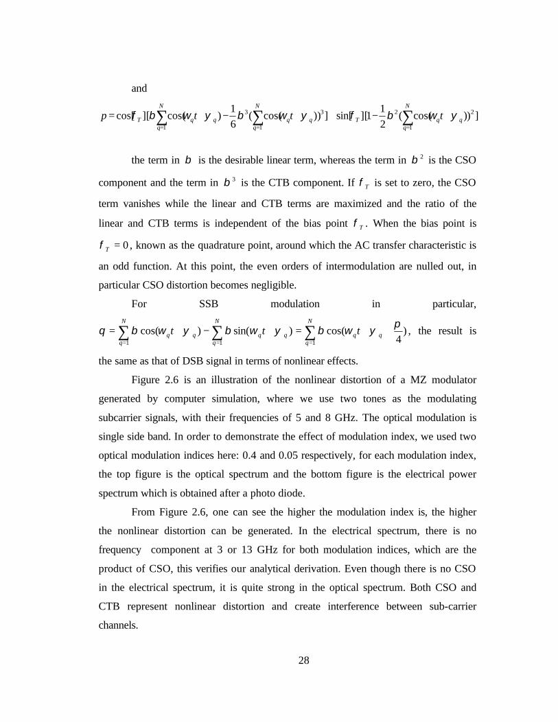
Figure 2.6 is an illustration of the nonlinear distortion of a MZ modulator

generated by computer simulation, where we use two tones as the modulating

subcarrier signals, with their frequencies of 5 and 8 GHz. The optical modulation is

single side band. In order to demonstrate the effect of modulation index, we used two

optical modulation indices here: 0.4 and 0.05 respectively, for each modulation index,

the top figure is the optical spectrum and the bottom figure is the electrical power

spectrum which is obtained after a photo diode.

From Figure 2.6, one can see the higher the modulation index is, the higher

the nonlinear distortion can be generated. In the electrical spectrum, there is no

frequency component at 3 or 13 GHz for both modulation indices, which are the

product of CSO, this verifies our analytical derivation. Even though there is no CSO

in the electrical spectrum, it is quite strong in the optical spectrum. Both CSO and

CTB represent nonlinear distortion and create interference between sub-carrier

channels.

29

Figure 2.6(a) is the optical spectrum with OMI of 0.4, Figure 2.6(b) is the

electrical spectrum with OMI of 0.4. Figure 2.6(c) is the optical spectrum with OMI

of 0.05, figure 2.6(d) is the electrical spectrum with OMI of 0.05. There is a trade off

between the signal amplitude and the distortion. The higher the modulation index is,

the higher is the signal amplitude, but the distortion is also higher. From the analytical

derivation, the ratio of the CTB terms over linear terms is independent of the bias

point Tφ and proportional to 2β .

0 5 10 15-100

-80

-60

-40

-20

0

20

Frequency (GHz)

Pow

er Spe

ctrum Density (d

Bm)

(a) optical spectrum of the MZ modulator output when OMI=0.4

0 2 4 6 8 10 12 14-100

-80

-60

-40

-20

0

20

40

Frequency (GHz)

Pow

er Spe

ctrum D

ensity (d

Bm)

(b) electrical spectrum of the photon dector output when OMI=0.4

Pow

er s

pect

rum

den

sity

(dB

m)

Pow

er s

pect

rum

den

sity

(dB

m)

30

0 5 10 15-100

-80

-60

-40

-20

0

20

Frequency (GHz)

Pow

er Spe

ctrum Density (d

Bm)

OMI=0.05

(c) optical spectrum of the MZ modulator output when OMI=0.05

0 2 4 6 8 10 12 14 16-100

-80

-60

-40

-20

0

20

Frequency (GHz)

Pow

er Spe

ctrum Density (d

Bm)

OMI=0.05

(d) electrical spectrum of the photon detector output when OMI=0.05

Figure 2.6 Illustration of nonlinear distortion of MZ subcarriers modulation

2.3.4 Carrier suppression

As shown in the section, the inter-modulation distortion can be reduced when

the optical modulation index (OMI) is small.

When the optical modulation index is small, the signal has a relatively large

carrier component and smaller signal components at subcarrier. In order to generate

enough signal to noise ratio, the signal component has to be as strong as possible and

the optical power of carrier could be very large. This is not very desirable since the

carrier power is not carrying any information. Further more, according to the study of

F.S.Yang [19], large carrier will result in some undesired effects:

Pow

er s

pect

rum

den

sity

(dB

m)

Pow

er s

pect

rum

den

sity

(dB

m)

31

1. For single wavelength, the SBS will clamp the input power and stoke wave will

increases the noise floor.

2. For WDM, stimulated Raman scattering (SRS) will deplete the power of high

frequency channel and generate interference on low frequency channels. XPM

will also lead to crosstalk between wavelength, both the SRS and XPM/GVD

crosstalk increase as 2Pc

So it is desirable to have less power in the carrier and more power in the

subcarriers. One way to accomplish this is to suppress the carrier component before

sending the signal into the fiber. It is worth noting that optical carrier suppression is

not useful in non-optically amplified systems because optical carrier suppression does

not increase baseband signal energy. In optically amplified systems, on the other

hand, without carrier suppression, EDFA output optical power would be limited by

the strong carrier component and therefore, carrier suppression will effectively

increase signal energy and increase receiver sensitivity.

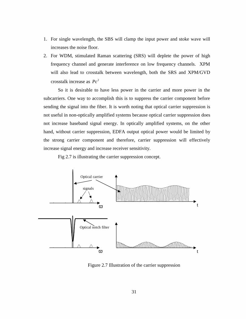
Fig 2.7 is illustrating the carrier suppression concept.

Figure 2.7 Illustration of the carrier suppression

ω t

Optical carrier

signals

ω

Optical notch filter

t

32

Fig.2.8 shows the experimental set-up for carrier suppression. A fabry-Perot

Interferometer (FPI) was used as a wavelength dependent reflector and an optical

circulator was used to re-direct the optical signal. The wavelength of the FPI was

tuned by its electrical bias in order to obtain an appropriate amount of carrier

suppression.

Figure 2.8, setup of the carrier suppression subsystem

The power transfer function of the Fabry-Perot interferometer is

τπfRR

RAfT

4cos21)1(

)(2

2

−+−−=

Here R is the power reflectivity (reflectance of each of the two mirrors). A is

the power absorption loss as the light passes through the cavity. The free spectral

range nx

cFRSR

221 ==τ

, the 3-dB or HPBW of the peak is given by

R

R

nx

c

R

RFSRHPBW

ππ−=−= 1

21

,

In the experiment, since you only the space between the two mirrors is

adjustable, so one can only change the wavelength of the peaks or nulls of the

spectrum. The suppression ratio can be changed by move the peaks close or further

away from the carrier component. In the simulation, to change the suppression ratio,

it is rather easy to keep the bandwidth of the filter unchanged and to change the

reflection loss A

FPI

Biascontrol

FPI reflection FPI transmission

Signal in

Signal out

33

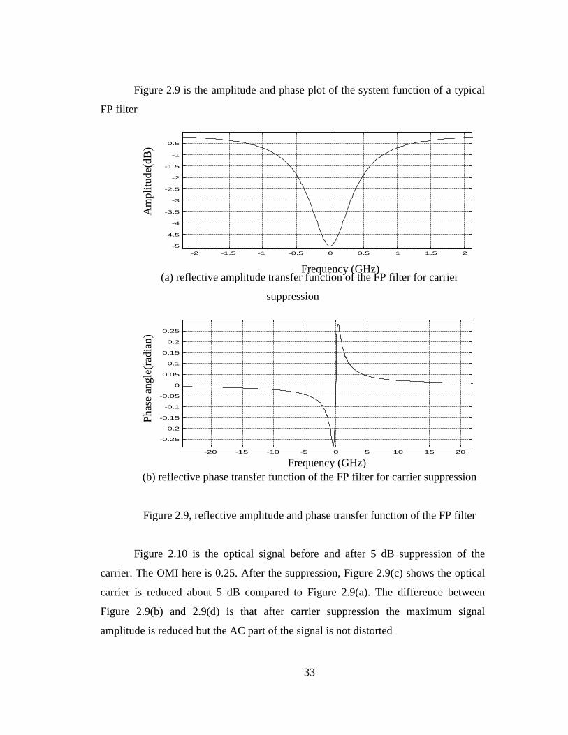
Figure 2.9 is the amplitude and phase plot of the system function of a typical

FP filter

-2 -1.5 -1 -0.5 0 0.5 1 1.5 2

-5

-4.5

-4

-3.5

-3

-2.5

-2

-1.5

-1

-0.5

(a) reflective amplitude transfer function of the FP filter for carrier

suppression

-20 -15 -10 -5 0 5 10 15 20

-0.25

-0.2

-0.15

-0.1

-0.05

0

0.05

0.1

0.15

0.2

0.25

(b) reflective phase transfer function of the FP filter for carrier suppression

Figure 2.9, reflective amplitude and phase transfer function of the FP filter

Figure 2.10 is the optical signal before and after 5 dB suppression of the

carrier. The OMI here is 0.25. After the suppression, Figure 2.9(c) shows the optical

carrier is reduced about 5 dB compared to Figure 2.9(a). The difference between

Figure 2.9(b) and 2.9(d) is that after carrier suppression the maximum signal

amplitude is reduced but the AC part of the signal is not distorted

Am

plitu

de(d

B)

Frequency (GHz)

Frequency (GHz)

Pha

se a

ngle

(rad

ian)

34

0 5 10 15 20 25

-60

-50

-40

-30

-20

-10

0TRANSMIT FILTER TOTAL SPECTRAL INTENSITY before FP

power spec

trum (dB

m)

Frequency (GHz)

(a) spectrum of the composite optical signal before the carrier suppresion

0.5 1 1.5 2 2.5 3 3.5 4 4.5 5

x 104

500

1000

1500

2000

2500

3000

3500

4000

4500

TRANSMIT FILTER OUTPUT PULSE --> INTENSITY before FP

Pulse

intensity (m

w)

Time (ps)

Carrier frequency=17.515 GHz

(b) waveform of the composite optical signal before the carrier suppresion

0 5 10 15 20

-45

-40

-35

-30

-25

-20

-15

-10

-5

0

TRANSMIT FILTER TOTAL SPECTRAL INTENSITY after FP

power spe

ctrum (d

Bm)

Frequency (GHz)

(c) spectrum of the composite optical signal after the carrier suppresion

Pow

er s

pect

rum

den

sity

(dB

m)

Inte

nsity

(ar

bitr

ary

unit

)

Pow

er s

pect

rum

den

sity

(dB

m)

35

0.5 1 1.5 2 2.5 3 3.5 4 4.5 5

x 104

0

500

1000

1500

2000

TRANSMIT FILTER OUTPUT PULSE --> INTENSITY after FP

Pulse

intens

ity (m

w)

Time (ps)

Channel Wavelength=1550 nm

Carrier frequency=17.515 GHz

(d) waveform of the composite optical signal after the carrier suppresion

Figure 2.10 Illustration of carrier suppresion: simulation spectrum and

waveforms

2.3.5 Transmitter optical filter

Because all the baseband information can be represented by only the upper

sideband, a transmitter optical filter can be used to further to filter out residual lower

sideband and limit the transmitter bandwidth. It can reduce crosstalk with other

wavelength channel in WDM configurations. The filter for this purpose is realized

using a Butterworth filter. This is because it has a smaller transition bandwidth

compared to the bessel filter. The bandwidth used here is 30GHz, and the order is 15.

Below is the spectrum before and after the optical filter, the intensity at –20 GHz is

decreased from –60 dBc to –100dBc, the intensity at 30 GHz is decreased from –60

dBc to –65dBc, thus when two wavelengths separated by 50 GHz multiplied together,

the crosstalk would be less than -100dBc.

Inte

nsity

(ar

bitr

ary

unit

)

36

-30 -20 -10 0 10 20 30

-50

-40

-30

-20

-10

0

10

20

30

Frequency (GHz)

Pow

er Spe

ctrum Den

sity (d

Bm)

(a) spectrum before the optical filter

-20 -10 0 10 20 30 40-100

-90

-80

-70

-60

-50

-40

-30

-20

-10

0

Spe

ctrum den

sity(dB)

Frequency (GHz)

(b) spectrum after the optical filter

Figure 2.11, signal spectrum before and after the WDM filter.

2.3.6 The post optical amplifier

The booster is to model the optical amplifiers that are used in the real systems.

We will not study the impact of the gain shape of the EDFA on the system

performance. We only use a flat gain EDFA in the simulation and the EDFA is

considered only with gain and noise. We do have an input parameter of noise figure,

but the noise of the EDFA is not numerically simulated but is calculated by an

Pow

er s

pect

rum

den

sity

(dB

m)

Pow

er s

pect

rum

den

sity

(dB

m)

37

analytical method. We will explain this later. Also, all the inline amplifiers are treated

the same way as the post amplifier.

38

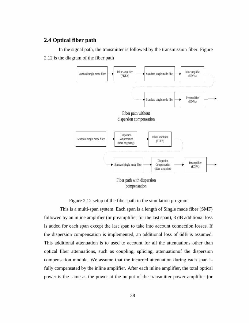
2.4 Optical fiber path

In the signal path, the transmitter is followed by the transmission fiber. Figure

2.12 is the diagram of the fiber path

Standard single mode fiberInline amplifier

(EDFA)Standard single mode fiber

Inline amplifier(EDFA)

Standard single mode fiberPreamplifier

(EDFA)

Standard single mode fiberInline amplifier

(EDFA)

Standard single mode fiberPreamplifier

(EDFA)

Fiber path withoutdispersion compensation

Fiber path with dispersioncompensation

DispersionCompensation

(fiber or grating)

DispersionCompensation

(fiber or grating)

Figure 2.12 setup of the fiber path in the simulation program

This is a multi-span system. Each span is a length of Single made fiber (SMF)

followed by an inline amplifier (or preamplifier for the last span), 3 dB additional loss

is added for each span except the last span to take into account connection losses. If

the dispersion compensation is implemented, an additional loss of 6dB is assumed.

This additional attenuation is to used to account for all the attenuations other than

optical fiber attenuations, such as coupling, splicing, attenuationof the dispersion

compensation module. We assume that the incurred attenuation during each span is

fully compensated by the inline amplifier. After each inline amplifier, the total optical

power is the same as the power at the output of the transmitter power amplifier (or

39

post amplifier). By adjusting the additional loss of the last span, we can change the

receiver power and find the receiver sensitivity. The sensitivity is defined as the

received power when the BER of 910− , or the Q value of 6.

Dispersion compensation is implemented by adding dispersion compensation

module at the end of each fiber span. The dispersion compensation module can be

made by DC fiber or fiber bragg gratings. Wehave neglected the nonlinearity of the

dispersion compensation components in our study.

The minimum fiber span length in the simulation is 40 km, the number of

span is calculated using ]lengthspan maximum

lengthfiber total[=N , ] [ means round to the

nearest integer toward 0. The fiber length of each span is calculated using

N

lengthfiber totallengthspan = . If the maximum span length is 80, by using such a

method, the resulting span length ranges from 40 to 80 km.

The fiber used in the simulation is standard SMF. Its loss factor is 0.25

dB/km, nonlinearity index is 2.36e-20 W/m2 , the effective area is 71 2um ,

dispersion parameter D= 18 ps/nm/km. Dispersion slope is 0.093 ps/nm^2/km, the

reason to select these parameter values is to find the worst case system performance.

We varied the PMD coefficient from 0.1 to 0.5 kmps / to evaluate its impact.

2.4.1 Nonlinear Schrodinger Equations

Optical fiber is one of the most important components in the whole system. It

contributes most to the signal distortion. Here we will introduce the nonlinear

propagation equation that governs the transmission characteristics. A numerical

method is used to integrate this equation.

Assume the solution of the optical field in the optical fiber has the form

40

)exp(),(~

),(),(~

000 zizAyxFE βωωωω −=−r , where ),( yxF is the transverse

filed. A is the complex envelope of the real signal amplitude. A is normalized such

that 2|| A represents the optical power. We then have a differential equation for A .

AAiAt

A

t

Ai

t

A

z

A 23

3

32

2

21 ||26

1

2γαβββ =+

∂∂+

∂∂+

∂∂+

∂∂

Here effcA

n 02ωγ = , is the nonlinear coefficient, 2n is the nonlinear refractive

index and effA is the effective fiber core area which depends on the distribution of the

transverse field in the fiber. iβ are coefficients of the Talor expansion of the mode

propagation constant )(ωβ , and we have 0

|)( ωωωββ ==

i

i

i d

d,

Wave propagation is sometimes referred to as the nonlinear Schrodinger

equation since it can be reduced to that equation under certain conditions.

There is a fundamental assumption in the above equation. We assume the

third order nonlinear effects (the nonlinear induced polarization) has an instantaneous

impulse response and it can be written by a product of three delta functions. So there

are some nonlinear effects can not be explained by this equation, such as stimulated

inelastic scattering like SRS and SBS. This equation is only valid for pulse widths

ps1.0≥ or a signal bandwidth of 1310 Hz. It will work fine in our simulation since

our total bandwidth is only in the order of 1110 Hz.

2.4.2 Numerical solution

Split step Fourier method is used extensively to solve the pulse propagation

problem in nonlinear dispersive media. Its fast speed can mainly be attributed to the

use of the fast Fourier transform algorithm.

The propagation equation can be written as

ANDz

A)ˆˆ( +=

∂∂

41

3

3

32

2

2 6

1

22

1ˆTT

iD

∂∂+

∂∂−−= ββα

( )2||ˆ AiN γ=

D is the differential operator that accounts for dispersion and absorption in a

linear medium and N is a nonlinear operator that accounts for the fiber

nonlinearities

Split step Fourier method obtains an approximate solution by assuming that

over a small distance h , the dispersive and nonlinear effects can be pretended to act

independently.

There are several variations of to implement this method. The most common

one is to use the following approximation

),()ˆexp()ˆexp(),()ˆˆexp(),( TzANhDhTzANhDhThzA ≈+=+

We ignored the non-commutating nature of the operators D and N , the

dominant error term is to the second order of the step size h . We will use this

approximation in our simulation program.

In the simulation, the step size h to satisfy the accuracy requirement. One

way to reduce the number of step is to utilize the fact that nonlinear distortion mainly

occurs at the beginning of the fiber where the optical power is high. At the end of the

fiber, due to the attenuation of the fiber, the optical power is low and the

nonlineareffect is thus low.

In our simulation, the step size is increased exponentially along the fiber, and

the exponential power number is the fiber attenuation.. At the beginning of the fiber

span the step size is smallest; at the end of fiber span, the step size is the largest. In

all the simulation, the number of steps per span used is 100 and there is no visible

change in the results with the increase of the number of steps.

Below is an exemplary spectrum after 80km standard SMF transmission with

complete dispersion compensation. The optical power launched into fiber is 3dBm,

42

and the Optical Modulation Index (OMI) is 0.4. After the fiber transmission, the

nonlinearity of fiber generates some new peaks on the other side of the carrier.

-20 -10 0 10 20 30 40-100

-90

-80

-70

-60

-50

-40

-30

-20

-10

0

Spe

ctrum den

sity(dB)

Frequency (GHz)

(a) spectrum before the optical fiber

-40 -30 -20 -10 0 10 20 30 40 50-100

-90

-80

-70

-60

-50

-40

-30

-20

-10

0

this is the spectrum after attenuation and dispersion of fiber

Spe

ctru

m d

ensi

ty(d

Bc)

Frequency (GHz)

=1 /sgth=1550 nm

(b) optical spectrum after 80 km fiber transmission

Figure 2.13 optical spectrum before and after 80 km fiber transmission,

optical power is 3dBm

Pow

er s

pect

rum

den

sity

(dB

m)

Pow

er s

pect

rum

den

sity

(dB

m)

43

2.5 SCM Receiver

Fig 2.14 is the diagram of the SCM receiver. In the receiver side, the EDFA

preamplifier output power of each wavelength is fixed at –5dBm for all the

simulations. The baseband electrical filters are the same as in the transmitter (6 orders

Bessel filters with 3dB bandwidth of 1.736 GHz). The frequencies of RF local

oscillators are 2.6GHz, 7.3GHz, 12GHz, and 16.7GHz respectively. The phases of the

local oscillators are estimated from the detected input signals. After the electrical

filter, we first estimate the total system delay and then search for the best sampling

time. The noise is calculated by an analytical method.

RF coupleropticaldetector

SCM Receiver Block Diagram

PreamplifierEDFA

Channel 1 RFoscillator(3.6GHz)

LPF

LPF

Q calculation

Q calculation

Synchronization

Synchronization

Channel 4 RFoscillator(17.5GHz)

WDMDemultiplexer

Figure 2.14 SCM receiver block diagram

2.5.1 optical demux

After transmission through the optical fiber, optical signal goes to a WDM

demultiplexer, it is used to select a single wavelength from the multiwavelength

44

lightwave signal. We used a Butterworth filter here as in the transmitter side. The

bandwidth is about 30GHz and the order is 6.

2.5.2 preamplifier

The optical demultiplexer is followed by an EDFA preamplifier (it may also

be put before the optical demultiplexer and this arrangement makes no difference in

our simulation). The output power from the preamplifier is fixed at –5dBm for each

wavelength. Once again, the amplifier has a flat gain and its ASE is calculated

analytically.

2.5.3 Photodiode

After the photo detector, the signal is transformed from a complex signal into

a real signal. The function of the photon detector is described by a square operation

and then followed by a low pass filter. Fig. 2.15 shows a spectrum of the electrical

current after the photon diode. The optical carrier beats with the optical sub carrierat

the photo diode, then the optical spectrum is shifted to an RF frequency as shown in

Fig. 2.15. The initially SSB optical spectrum is converted to a DSB RF spectrum

because of the square-law process of the photo diode.

In practice, there is always an electrical preamplifier after the photo diode, we

didn’t include it here thus the noise generated by the electrical circuit is neglected.

-30 -20 -10 0 10 20

-100

-90

-80

-70

-60

-50

-40

-30

Frequency (GHz)

Pow

er S

pectrum D

ensity (d

Bm)

Figure 2.15, electrical spectrum after the photon detector

Pow

er s

pect

rum

den

sity

(dB

m)

45

2.5.4 High pass filter

In Fig. 2.15, we can see that there is a very high DC component. Since the DC

component doesn’t carry any information, it could be removed. Another reason why

we need to remove the DC component is that later during the RF coherent detection,

this DC component will move to a nonzero frequency and will interfere with the

signal. It will be hard to be removed at that time because of the filter can not be made

with very high extinction ratio. In the simulation, we use a high pass RF filter to

remove this DC component, the filter is a 5 MHz, 6 order Butterworth high pass filter.

In real implementation, this could be done simply by using a capacitor to couple the

signal. Figure 2.16 is showing the spectrum after the filter.

-30 -20 -10 0 10 20 30

-130

-120

-110

-100

-90

-80

-70

Frequency (GHz)

Pow

er Spec

trum D

ensity (d

Bm)

Figure 2.16, electrical spectrum after the high pass filter

2.5.5 Microwave coupler.

A 1×4 microwave (RF) coupler is needed in order to separate four subcarrier

channels. The attenuation of the microwave coupler is not considered in the

simulation because the SNR is determined before the microwave coupler.

2.5.6 Carrier recovery

After the microwave coupler, the signal at each subcarrier branch is mixed

with a local oscillator. The frequencies of local oscillators are the same as they are in

Pow

er s

pect

rum

den

sity

(dB

m)

46

the transmitter side. The phase of the local oscillator is a very important variable to

be determined here. Suppose one of the subcarrier is )cos(*)( φω +ttA , the phase of

the local oscillator is Lφ , then the useful output signal would be )cos()( LtA φφ − , if

2/πφφ =− L , then the output signal would be 0.

In practice, the phase of the local oscillator can be estimated by methods such

as phase lock loop or Mth Power loop. In the simulation, we use the Mth Power loop.

The Mth Power loop is also referred to as the squaring loop. It can be applied

to MPSK signal. The MPSK signal can be represented by

)2cos()( θθπ ++= kctfAts . During SS TktkT )1( +≤≤ , where ST is the symbol

length and kθ is the angle corresponding to the kth transmitted symbol. kθ has one of

the M values. M

MMMMk

ππππθ 2)1(,.....,

23,

22,

2,0 −= . θ represent the phase delay due

to the transmission and processing. Now if we raise )(ts to the power M, and use the

fact that kMθ is integer multiple of π2 , then we have

sother term)2cos(

sother term)2cos()(

++=

+++=

θπθθπ

MtMfA

MMtMfAts

cM

kcMM

The first term is first extracted by a bandpass filter and then a frequency

divider.( by a factor of M) can be used to generate a local carrier of the form

)2cos()( θπ += tfKtC c ,

In the simulation, there is another possible choice to get the exact phase of the

received carrier. First, the total delay of the optical fiber can be calculated then the

effect of transmitter bias is added which is a random delay for the baseband signal of

each subcarrier. From this delay, one can calculate the exact timing of the received

signal and fine the phase of the carrier. However, we found that this method is not

accurate enough to get a good estimation of the phase due to numerical accuracy.

When the Mth Power loop method is used, the frequency divider is not easy to

simulate. One way to get around it is to use the cross-correlation method. From the

cross correlation of the filtered Mth harmonic from the Mth loop and an ideal Mth

47

harmonic, it is possible to find a peak that correspond to the M times exact phase shift

of the received carrier. Dividing this phase by M, the exact phase of the received

carrier can be obtained.

Figure 2.17(a) is a diagram of the carrier recovery scheme for BPSK system.

A bandpass filter is used to select a single subcarrier. This single subcarrier signal is

squared by a mixer and then the second order harmonics of the product is selected by

a narrow bandpass filter. At last, a frequency divider is used to get the desirable

carrier for this subcarrier. Figure 2.17(b) are the waveforms corresponding to those

points in the diagram.

bandpass filterfor subcarrier

compositeRF signalsafter thephotondetector

mixer

narrow bandpassfilter

for second orderharmonics

frequencydidvider

recoveredsubcarrier

(a)(b)

(d)

(c)

(e)

Figure 2.17 (a) diagram of the carrier recovery for BPSK system

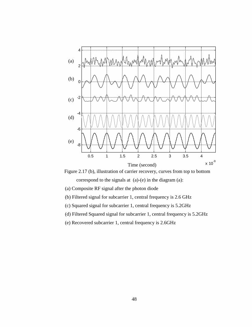
48

0.5 1 1.5 2 2.5 3 3.5 4

x 10-9

-8

-6

-4

-2

0

2

4

Figure 2.17 (b), illustration of carrier recovery, curves from top to bottom

correspond to the signals at (a)-(e) in the diagram (a):

(a) Composite RF signal after the photon diode

(b) Filtered signal for subcarrier 1, central frequency is 2.6 GHz

(c) Squared signal for subcarrier 1, central frequency is 5.2GHz

(d) Filtered Squared signal for subcarrier 1, central frequency is 5.2GHz

(e) Recovered subcarrier 1, central frequency is 2.6GHz

Time (second)

(a)

(b)

(c)

(d)

(e)

49

2.5.7 Demodulation

Fig. 2.18 shows the spectrum at the received signal after the mixer, which

performs the RF coherent detection.

-30 -20 -10 0 10 20 30

-70

-60

-50

-40

-30

-20

-10

0

OUTPUT OF SCM Demodulator before filter --> chan1 Spectrum

Spe

ctrum den

sity(d

B)

Frequency (GHz)

Number=1

2.48 Gb/s

Wavelength=1550 nm

Figure 2.18, signal spectrum after beating with local ossillator

In reality, the output port of the mixer has a certain banwidth, in the

simulation we used a 6-order Butterworth low pass filter with a bandwidth of 1.25

times the bitrate. Fig. 2.19 shows the spectrum, waveform and eyediagram after this

filter. The eye diagram here is shifted to all positive in Fig2.19(c), this is only for the

convenience of comparasion.

-8 -6 -4 -2 0 2 4 6

-60

-50

-40

-30

-20

-10

0

OUTPUT OF SCM Demodulator after filter --> chan1 Spectrum

Pulse

intens

ity (m

w)

Frequency (GHz)

(a) spectrum of the mixer output

Pow

er s

pect

rum

den

sity

(dB

m)

Pow

er s

pect

rum

den

sity

(dB

m)

50

0.5 1 1.5 2 2.5 3 3.5 4 4.5 5

x 104

-0.08

-0.06

-0.04

-0.02

0

0.02

0.04

0.06

0.08

0.1

OUTPUT OF SCM Demodulator --> INTENSITY

Pulse

amplitu

de (m

A)

Time (ps)

Channel Number=1 Bit Rate=2.48 Gb/sChannel Wavelength=1550 nmCarrier frequency=3.6038 GHz

(b) waveform of the mixer output

200 400 600 800 1000 1200 1400 1600 1800

0

0.02

0.04

0.06

0.08

0.1

0.12

OUTPUT OF SCM Demodulator --> EYE DIAGRAMS

Pulse amplitude

(mA)

Time (ps)

(c) eyediagram of the mixer output

Figure 2.19 spectrum, waveform and eyediagram of the mixer output

2.5.8 Electrical filters

As the bandwidth of the mixer is larger than the signal bit rate, the signal at

the mixer output is still distorted by the crosstalk of other subcarriers. We need

another narrower baseband to purify our final signal. This electrical filter is the same

as that used in the transmitter (6-order Bessel filters with 3dB bandwidth of 1.736

GHz). Fig. 2.20 shows the spectrum, waveform and eyediagram respectively, after the

baseband filter. The spectrum shows that the side band here is furthered suppressed

compare to the previous spectrum and the eye diagram looks cleaner.

Puls

e am

plitu

de (

mA

)Pu

lse

ampl

itude

(m

A)

51

-4 -3 -2 -1 0 1 2 3 4-120

-110

-100

-90

-80

-70

-60

Frequency (GHz)

Pow

er Spectrum Density (dBm)

(a) spectrum after electrical filter

0.5 1 1.5 2 2.5 3 3.5 4 4.5 5

x 104

0

0.02

0.04

0.06

0.08

0.1

0.12

RECEIVER ELECTRIC FILTER --> PULSE INTENSITY:

Pulse

amplitu

de (m

A)

Time (ps)

(b) waveform after electrical filter

200 400 600 800 1000 1200 1400 1600 1800

0

0.02

0.04

0.06

0.08

0.1

0.12 RECEIVER ELECTRIC FILTER --> EYE DIAGRAM:

Pulse amplitude (mA)

Time (ps)

(c) eyediagram after electrical filter

Figure 2.20, spectrum, waveform and eyediagram after electrical filter

Puls

e am

plitu

de (

mA

)Pu

lse

ampl

itude

(m

A)

Pow

er s

pect

rum

den

sity

(dB

m)

52

2.5.9 Bit Synchronization procedure

After the electrical filter, there is another synchronization procedure that

estimates the decision timing of the digital signal. This estimation is based on the

delay of the transmission through the optical fiber. Although it does not have to be as

accurate as for the estimation of the carrier phase, it needs to be adequate enough.

Suppose the absolute frequency of the chosen subcarrier is if , (the frequency

shift from the zero or the reference frequency of the simulation. This is the frequency

of the wavelength channel plus frequency of the subcarrier within that wavelength

channel). The delay can be calculated as LDfc io ***/2λ , where oλ is the center

wavelength of the simulation which is 1550nm. c is the speed of light, D is the fiber

dispersion parameter at frequency if . L is the length of the fiber. If there is

dispersion compensation in the fiber path, the average value of D has to be changed

accordingly by the ratio of the dispersion compensation. Also, the dispersion slope

should be considered here too.

2.5.10 Polarization effects in SCM system

2.5.10.1 Polarization walkoff

Optical fiber is not purely a polarization independent transmission media, it

has polarization-related effects such as polarization mode dispersion (PMD) and

polarization dependent loss (PDL). We will consider the PMD effect here.

In frequency domain, PMD manifests as a frequency dependency of signal

polarization at the output of a fiber, the output polarization undergoes a rotation on

the Poincare sphere that can be represented by the following differential equation,

sd

sdˆ

ˆ⊗Ω=

ω, where s is the unit Stokes vector describing the output polarization

state, Ω is the rotation vector, which describes the rate of rotation and is also referred

to as the dispersion vector. The magnitude of the Ω vector is equal to the differential

delay time: τ∆=Ω and the direction of this vector defines an axis whose two

53

intercepts with the surface of the Poincare sphere correspond to the two principal

states of polarization at the fiber output.

In general, both the differential delay and the dispersion vector, Ω , are

themselves frequency dependent and may vary over the bandwidth of a signal source.

If the first order PMD is considered, Ω can be treated as frequency independent.

When the second order dispersion PMD is included, in the frequency domain, it

manifests as a linear frequency dependence of the dispersion vector Ω .

In our study, we only consider the first order PMD. The frequency of the

highest subcarrier is lower than 20GHz and the wavelength change between the

highest subcarrier and the carrier is not considered to be very large. So we can assume

the principal state remains fixed for carrier and subcarriers (the Ω is fixed). The

differential group delay can be written as ωθτ

∆∆=∆ , where the τ∆ is the differential

group delay (DGD) in seconds, θ∆ is the rotation about the principal states axis in

radians, and ω∆ is the optical frequency change that produced this θ∆ rotation, ω∆

has a unit of radians/second.

As a first order estimation, in a SCM system that needs the carrier to beat with

the subcarrier in the photo diode to reproduce RF signal, the polarization walkoff

between the carrier and subcarrier will decrease the amplitude of the signal at the

output of the photo detector by a factor of )cos( θ∆ . θ∆ is the rotation angle between

the carrier and the subcarrier. Because of PMD, the beating between the carrier and

the subcarrier will generate less microwave signal due to the polarization

misalignment between each other in the photon diode.

In the simulation, this walkoff problem is modeled as a reduction in the signal

amplitude by a factor of )cos( θ∆ .

2.5.10.2 Polarization mode dispersion

PMD also has another detrimental effect on the SCM system. It will distort the

microwave signal at the photon detector when the optical signals in two polarization

54

modes combine together just like in traditional high speed TDM systems. At the fiber

output, the signal can be divided into two main polarization modes, these two modes

have different transmission delay due to PMD. The higher frequency subcarrier

channel will be more subject to PMD effect because the period of that subcarrier is

small. We will use the same method, which was used to estimate the PMD effect in

binary systems to estimate the PMD effect in SCM systems [18].

To evaluate the impact of PMD in a binary digital system, one usually

assumes that pulse bifurcation is the dominant mechanism for pulse broadening. The

goal here is to find the maximal allowable mean DGD or τ∆ that can ensure the

system outrage probability larger than 1 dB system penalty to be less than 30 min per

year. We assume a Maxwellian distribution for τ∆ and uniform distribution for the

power splitting ratio between the two orthogonal state of polarization (SOP). From

those assumptions, for a digital system with Chirp Free Gaussian pulses, the DGD

between the principal states must be less than 0.14 of the bit period, i.e.,

14.0<=>∆<T

τ. For a binary system, this can be written as

22

)(

020.0

PMDLB ≈ [18],

where B is bit rate, L is the fiber length, PMD is the PMD coefficient .

For SCM systems, the subcarrier is sinusoidal and we assume that has the

similar performance compared to a Gaussian pulse. It would be appropriate to

substitute B with if , which is the subcarrier frequency. Based on this assumption,

Figure 2.21 is the estimation of the limitation on SCM system due to the PMD effect.

The upper trace is obtained when the sub carrier frequency is 12 GHz and the lower

trace is obtained when the sub carrier frequency is 18GHz. The horizontal axis is the

PMD parameters. The vertical axis is the maximum transmission distance.

With G.652 SMF, the PMD parameter is <=0.5 kmps / . For some newly

installed fiber cables, the PMD parameter could be <=0.1 kmps / . When the PMD

is 0.5 kmps / , the distance limits are appropriately 240km and 550km respectively

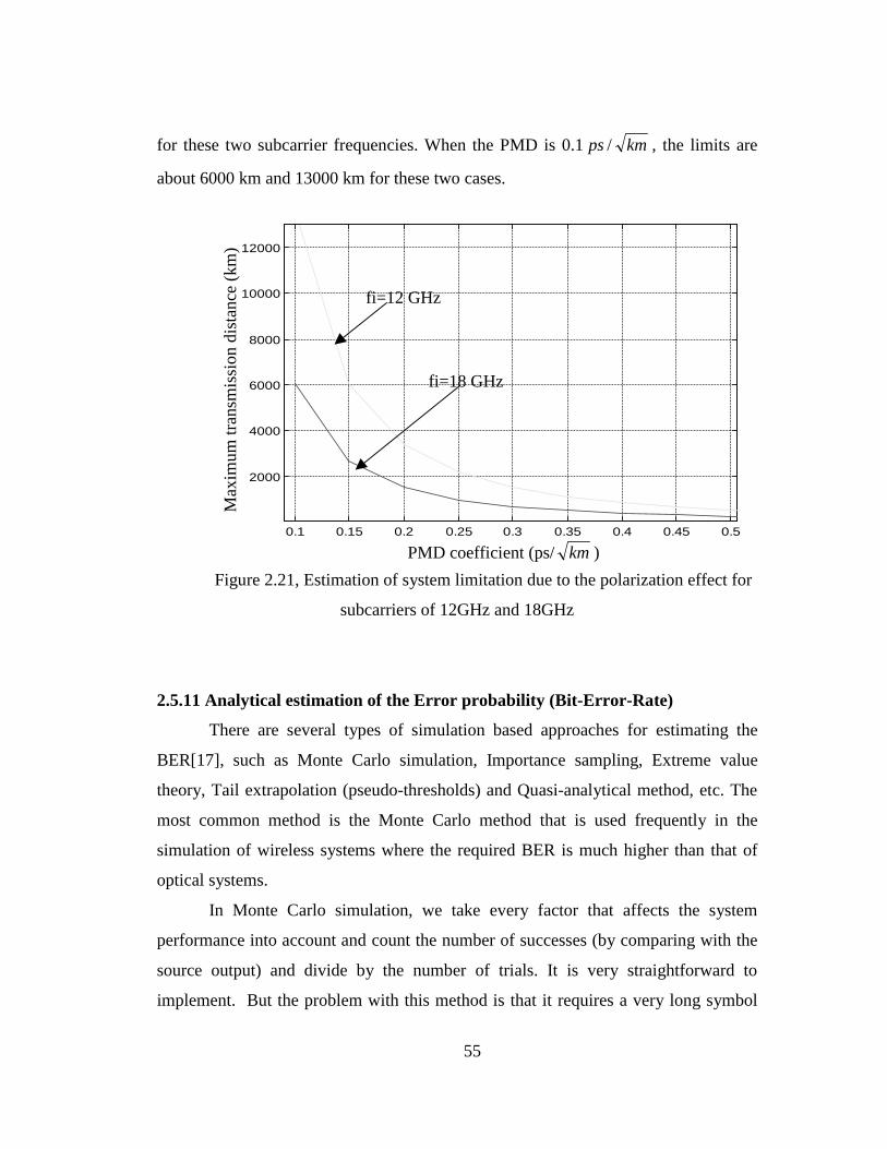
55

for these two subcarrier frequencies. When the PMD is 0.1 kmps / , the limits are

about 6000 km and 13000 km for these two cases.

0.1 0.15 0.2 0.25 0.3 0.35 0.4 0.45 0.5

2000

4000

6000

8000

10000

12000

Figure 2.21, Estimation of system limitation due to the polarization effect for

subcarriers of 12GHz and 18GHz

2.5.11 Analytical estimation of the Error probability (Bit-Error-Rate)

There are several types of simulation based approaches for estimating the

BER[17], such as Monte Carlo simulation, Importance sampling, Extreme value

theory, Tail extrapolation (pseudo-thresholds) and Quasi-analytical method, etc. The

most common method is the Monte Carlo method that is used frequently in the

simulation of wireless systems where the required BER is much higher than that of

optical systems.

In Monte Carlo simulation, we take every factor that affects the system

performance into account and count the number of successes (by comparing with the

source output) and divide by the number of trials. It is very straightforward to

implement. But the problem with this method is that it requires a very long symbol

PMD coefficient (ps/ km )

Max

imum

tran

smis

sion

dis

tanc

e (k

m)

fi=12 GHz

fi=18 GHz

56

sequence. If the BER is p , the sequence length N should be on the order of p/10 ,

and it will produce a 95% confidence that the real BER will be between (1.8* p to

0.55 p ), you will see how long it will take for a BER of 910− . Most other methods

are derived from the Monte Carlo method. They produce many more errors per unit

time by altering the statistical properties of the noise processes (importance sampling)

or by change the decision threshold (Tail extrapolation). But all these methods are

relatively difficult to be implemented.

In the simulation, we have used a Quasi-analytical method to estimate the

BER. Quasi-analytical (QA) technique is also referred to as semi-analytic. Basically,

the QA technique is hybrid in that it combines both numerical simulation and

analytical analysis. The simulation is used to generate a noiseless waveform with

distortion at the receiver. Given this waveform and assuming that the noise is additive

and has a known pdf, one can then calculate the probability of errors with analytical

formulas. This is the analytic portion.

The advantage of this method is time efficiency. We don’t have to wait for

enough errors to occur and we can use much shorter symbol sequence.

In most other BER estimation methods, the waveform contains all of the

effects of the system, acting simultaneously on signal and noise. In the QA method

we separate the problem into two parts, one dealing with the signal wavelength and

the other with the noise contribution to the sampled waveform. We assume all the

noise can be considered additive at the input of the decision device, irrespective of

how many noise sources there are in the actual system or where they generated. The

probability density function of the noise may be specific for different system

configurations.

If we know the pdf of the noise is Gaussian, and the decision value DI is

chose such that QII

QII

Q DD =−==−=0

00

1

11 σσ

, we have01

0110

σσσσ

++= II

I D is the

optimum decision threshold. 1I is the minimum of symbol “1” and 0I is the

57

maximum of symbol “0” at the decision time, 0σ and 1σ are the noise variance at

signal zero and ones respectively. In the simulation, 1I and 0I were obtained by

numerical simulation of the system, 0σ and 1σ were calculated by the analytical

equations. With the values of1I , 0I , 0σ and 1σ known, we can find

)2

(2

1 QerfcBER = where

01

01

σσ +−

=II

Q .

In the simulation, the receiver sensitivity can be obtained with the knowledge

of eye opening and noise. The sensitivity is defined as the minimum optical power to

achieve BER=10e9− or Q=6. The sensitivity can be found by changing the

attenuation of the last fiber span. When the input power to the EDFA preamplifier

changes, the gain of the amplifier will also change to keep EDFA output to be

constant. As will be discussed in the next section, when the EDFA gain changes, the

ASE noise will also change. So when the input signal optical power is decreased, the

noise will increase and finally there is a point that the noise variance is big enough to

make Q=6, this point is our receiver sensitivity.

2.5.12 Calculation of Receiver sensitivity

In an optical communication system with optical amplification, the receiver

noise comes from both photo diode and optical amplifiers. In optically pre-amplified

receiver, signal-ASE beat noise is usually the dominant noise that leads to

performance degradation. We only consider the beat noise in our studies.

2.5.12.1 Noise from optical amplifier

In a long haul transmission system, the use of optical amplifier is inevitable

and the noise generated by optical amplifiers is the dominant factor that contributes to

the SNR degradation [15]. This noise is commonly referred to as the amplified

spontaneous emission (ASE) noise. The optical spectral density of ASE has wide

bandwidth (white noise) and is given by )1(2)( −== GhfnfS ospASEASE ρ , the factor

58

2 accounts for two polarizations. Here of is the optical frequency, spn is the

spontaneous emission factor which is given by 12

2

NN

Nnsp −

= , 1N and 2N are the

carrier populations at the ground and excited states. The major effect of the ASE

noise is that it beats with the signal during the O/E conversion and generates RF noise

in the photo current. The noise figure of the amplifier can be expressed as

spspn nGGnF 2/)1(2 ≈−= , we can calculate spn through 10/)3(10 −= nFspn if we know

nF

The electrical spectrum of signal-spontaneous-beat noise is given by

ASEininspspsig GPRGGPnhf

qfS ρη 2

22

2)1(4)( =−=− (single-side band spectrum), here

we have considered that the signal only has one polarization and the ASE noise has

two. In addition, ASE noise will also beat with itself and generate spontaneous-

spontaneous-beating noise oASEospspsp BRBGnqfS 222222 )2/1()1(2)( ρη =−=− , where

oB is the bandwidth of the optical filter before the receiver. We should note that the

signal spontaneous beat noise is independent of the optical bandwidth oB while the

spontaneous-spontaneous beat noise is a function of the optical bandwidth. We can

not use an optical filter to eliminate signal- spontaneous beat noise. This is because

there is always a beat noise between signal and ASE which falls into a bandpass or

baseband filter in a receiver and one cannot eliminate this beat noise without

eliminating the desired signal at the same time. On the other hand, the spontaneous-

spontaneous beat noise is the result of beating among ASE components and is

proportional to oB , which means that the narrower the optical filter is the less the

noise is. This noise is usually much smaller than the signal-spontaneous-beating

noise. The noise current variance can be expressed by eASEinsps BGPR ρσ 22 2=− and

eoASEspsp BBR 222 )2/1( ρσ =− , for signal-ASE and ASE-ASE beat noise, respectively,

where eB is the bandwidth of the baseband filter.

59

When several concatenated amplifiers are used, ASE noise generated by each

amplifier has to be added together.

2.5.12.2 Sensitivity estimation for a digital BPSK SCM system:

In this section, we give an analytical estimation of the receiver sensitivity for

digital SCM system. We only consider the EDFA preamplifier here and neglect the

noise from optical detector and the electrical amplifier.

Fig. 2.22 shows the block diagram of an optically amplified, digital SCM

fiber-optic system.

Figure 2.22 , concept model of the SCM system for Q calculation

In the transmitter side, suppose that the electrical modulation index M = 100%

and the optical modulation index is m. For a Mach-Zehnder modulator, the transfer

function of the optical field is proportional to the input RF signal in a nonlinear way,

E Ev t

Vi b0 2= +

sin

( )πϕ

π

where v(t) is the electrical signal used to modulate the CW optical input EI. φb

is a constant phase, which depends on the bias point of the modulator.

For a multiple sub-carrier signal, we have,

)cos()()()(11

ttuvtvtv k

n

kkk

n

kk ω∑∑

==

==

m

M

Pin EDFAEDFA

Laser Modulator

DigitalData

RF Carrier

G LPFFiber

Preamplified optical receiver

GPin, ρase

60

Where uk(t) is the normalized digital signal at the kth channel with uk(t) = -1

and uk(t) = 1 representing digital signal “0” and “1”, respectively and ωk is the carrier

frequency of that channel. If φb = π/4, which corresponds to biasing the modulator at

the quadrature point, we have

+

= ∑∑

==

n

kkkk

n

kkkk

i ttuvv

ttuvv

EE

110 )cos()(

2cos)cos()(

2sin

2ωπωπ

ππ

Under the assumption of v(t) << Vπ, this expression can be linearized,

+= ∑=

n

kkkk

i ttuvv

EE

10 )cos()(

21

2ωπ

π

Here the first term in the bracket represents the carrier and the second term is

the signal. Taking into account the carrier suppression,

+= ∑=

n

kkk

ki ttumE

E1

0 )cos()(22

ωζ

Where ζ is the power suppression ratio of the carrier and mk is the modulation

index of the kth channel and this modulation index is defined by the percentage of the

RF signal voltage compared to the modulator’s Vπ parameter. At the receiver, the

photo-current is

+≈ℜ= ∑=

n

kkkks ttumIGEI

10

20 )cos()(

11 ω

ζη

Where η is the system loss, ℜ is the photo-diode responsivity, G is the gain

of the optical pre-amplifier, ( ) ℜ=ℜ= GPGEI ini ζη 20 2/ is the photo-current and

P Ein i= η ζ( / )2 2 is the average power of optical signal that reaches the pre-

amplified optical receiver. Obviously, the useful signal photo-current for the kth

channel is ζω /)cos()( ttumGPI kkkink ℜ= .

On the other hand, GPi inasespsig ρ222 ℜ=− is the power spectral density of

signal-spontaneous beat noise. oASEspsp Bi 222 )2/1( ρℜ=− is the spectral density of

61

spontaneous-spontaneous beat noise, where oB is optical filter bandwidth and ASEρ is

the ASE noise spectral density. Although there are other receiver noises such as

thermal noise and shot noise, for optically pre-amplified receiver, signal-spontaneous

beat noise is the dominant noise. Therefore, for simplicity, we only take into account

the signal-spontaneous beat noise here.

Since the noise is random, it can be decomposed into in-phase component

)(tnc and quadrature component )(tns and thus the total AC signal entering the RF

demodulator is )sin()()cos()(/)cos()(1 ttnttnttumGPU kskckkkin ωωζω ++ℜ=

Where the total noise power is

einasespsigesc GBPiBnn ρ2222 22

1

2

1 ℜ>=<=+ − , and 22sc nn =

Be is the bandwidth of the receiver baseband electrical filter.

At the demodulator, U1(t) coherently mixes with a local oscillator 2cos(ωkt),

the output of the demodulator is:

U P G m u t n tin k k c2 = ℜ +( ) / ( )ζ

Here frequency-doubled components have been filtered out. Therefore the

signal-to-noise-ratio is

SNRP G m u t

P GB

P G m u t

P Fh G GB

u t P m

Fh Bin k k

in ase e

in k k

in e

k in k

e

=ℜ

ℜ=

ℜ

ℜ −≈

( ) / ( ) /

( )

( )ζ

ρ

ζ

υ υ ζ2 2 1 22 2

2

Taking into account the fact that )1,1()( −∈tuk , therefore, without signal

waveform distortion, the receiver Q value can be approximated as

Qm P m P

Fh B

m P

Fh Bk in k in

e

k in

e

=− −

=( )1

2 2 2υ ζ υ ζ

A BER of 10-9 corresponds to Q = 6, therefore the receiver sensitivity at this

BER level is PF B

mine

k

=× × × −36 2 128 10 19

2

. ζ

62

In the ideal case without waveform distortion, suppose the receiver electrical

bandwidth is 1.75GHz, optical preamplifier noise figure is 3 (~5dB), modulation

index is 25% which is the maximum index for a system with 4 subcarrier channels

and there is no carrier suppression, the sensitivity is about -31dBm.

2.5.12.3 Sensitivity Evaluation for QPSK SCM system:

In a QPSK system, for a multiple sub-carrier signal, we have

∑∑==

+==n

kkQkkkIkk

n

kk ttuvttuvtvtv

11

)sin()()cos()()()( ωω

Where )(tuIk and )(tuQk are the normalized digital signal for I and Q

baseband channels of the kth subcarrier channel. Similarly as BPSK system, at the

receiver, the photo-current is

++≈ℜ= ∑=

n

kkQkkIkks ttuttumIGEI

10

2

0 )sin()()cos()(1

1 ωωζ

η ,

we note that the peak to peak value of modulating signal for each subcarrier

)sin()()cos()( ttuttu kQkkIk ωω + is 2 times of that of )cos()( ttu kk ω in BPSK, in a

system with only 2 QPSK subcarriers, the maximum km should be

2*25.02/2*25.0 = , the 2 factor here is to account that there are only 2

subcarriers here and we can double the modulation index for each subcarrier, the 2

factor here is to account the difference on the peak to peak value of the modulating

signal for each subcarrier for QPSK and BPSK.

The noise calculation for QPSK is the same as BPSK. So a 2 subcarriers

QPSK system will have 3 dB improvement on the sensitivity comparing to a 4

subcarriers BPSK system. The sensitivity would be –34 in this case.

2.5.12.4 Sensitivity Evaluation for a binary ASK system:

This section considers both the optically filtered ASK SCM system and the

traditional IMDD system. If we only consider one subcarrier in a ASK SCM system,

63

these two systems essentially have the same signal to noise ratio since they have the

same detection schemes. The only difference in their modulation is that ASK SCM

system has a carrier component. However, this carrier can be suppressed or removed.

Signal spontaneous beat noise is given by

)1(2)( −== GhfnfS ospASEASE ρ ,

ASEininspspsig GPRGGPnhf

qfS ρη 2

22

2)1(4)( =−=− , here we have considered

that the signal only has one polarization and the ASE noise has two.

)0()1(

)0()1(

tottot

SS

NN

IIQ

+−= , Suppose that there is no waveform distortion and

signal spontaneous beat noise is the dominant noise. Q can be reduced to

speo

in

einspo

in

nBhf

P

BGGPnhfR

RGPQ

2)1(24

22

=−

= , here the factor 2 before the Pin is

because that the average power is half of that of the mark power.

When Q is 6 which corresponding to a BER of 910− , the sensitivity of OC48

and OC192 binary system is about –46 and –40 if the bandwidth of the electrical filter

is only 0.7 times of the bit rate.

64

Chapter Three

Simulation results of SCM systems

In the last chapter, we have described the basic simulation setup for a 4

subcarriers BPSK system. We also discussed some particular issues for the SCM

system and its simulation. Based on the basic setup described in the last chapter, we

will use the simulation model to study the performance of three types of SCM system:

4 subcarriers BPSK system, 2 subcarriers QPSK system, 4 subcarriers ASK system.

We will also present the result for a traditional OC192 system as a comparison.

First we will make the selections of basic simulation parameters in this

chapter, such as the modulation index, RF frequency allocation plan, the bandwidth

of the filters etc. This optimization is not necessarily the best, however it will give a

possible range within which the system may perform better than out of this range. Or

it will give guidance when select the parameters.

It has to be mentioned that there are many factors that are not included or

considered in our simulation while they exist in reality, such as the gain tilt of the

EDFA, the frequency or wavelength dependence of the dispersion compensation

modules etc. Second, though we don’t consider all the parameters in a real system,

the number of parameters that are considered in the simulation is still large and the

combination of different values is huge. We can not simulate all those combinations.

We will only consider some meaningful combinations.

After we have some basic idea about how to choose the parameters, we will

use one set of the values to find out the performance of an optimized SCM system

under different situation such as fiber with different PMD coefficient, with or without

dispersion compensation.

As mentioned in the last chapter, we will only study Standard single mode

fiber systems because it is most commonly used by large telecos like AT&T, Sprint

and Worldcom. Usually newer SMF will have better PMD coefficient which is

65

typically less than 0.1 ps /sqrt(km) while old SMF may have PMD coefficient as high

as 0.5 ps /sqrt(km). Since the SCM systems are sensitive to the PMD effects, we will

study fibers with these two different PMD values.

In the next chapter, we will introduce the experiment that we did in the lab,

which is a system with 4 BPSK subcarriers. We will discuss the result and compare it

with the simulation.

3.1 Performance of an SCM system using 4 BPSK subcarrier each

with OC48 data, and with self-coherent detection

In the receiver, if the optical carrier is used to beat with the subcarrier and the

subcarrier is demodulated coherently, we will call it a self-coherent detection. We

will first study the performance of a SCM system with 4 BPSK subcarriers per

wavelength. Each of the subcarriers will carry data at the rate of OC48. This system is

the simplest system in the three types of systems we considered in this study. It has

simpler modulation format comparing to QPSK system. Compared to direct detection

system, it does not require narrow band optical filters. However, we also will see that

its performance is the worst in the 3 types of systems.

3.1.1 Bandwidth of the electrical filters

One system parameter is the bandwidth of the baseband electrical filters that

are used in the transmitter and the receivers. The wider the bandwidth, the more

information the system can preserved and the better eye-opening can be expected, but

obviously, less channels could be packed into the same system. In most digital

communication systems, the filters bandwidth are set as ratebit *75.0 , for example,

for an OC48 system, the filter bandwidth will be 1.86 GHz, and the double side

bandwidth is 3.72GHz.

We did a simulation on the effects of the filter bandwidth. In the simulation,

the channel spacing between subcarriers is fixed at 4.7 GHz which is about 2 times of

the bit rate. Then the bandwidth of the baseband filter is changed from 1 times the bit

66

rate to 0.4 times of the bit rate. The bandwidths of all the filters are the same in

transmitter and receiver. The filters used in the simulation are 6 order butterworth

filters. The plot below shows the worst sensitivity of the 4 RF channels vs. the filter

bandwidth factor.

0.2 0.3 0.4 0.5 0.6 0.7 0.8 0.9 1-32

-30

-28

-26

-24

-22

-20

-18

Figure 3.1, worst sensitivity of the 4 subcarrier channels vs. the filter

bandwidth factor

From this plot, the best factor is 0.7. In last chapter, we derived an expression

of receiver sensitivity. It is shown that the sensitivity is inversely proportional to the

bandwidth of the electrical filter. The larger the bandwidth, the more noise is picked

up by the receiver. On the other hand, if bandwidth is too small, the signal itself is

distorted because the useful information is filtered out. From now on, we will use 0.7

as the factor for the filter in our simulation.

Filter bandwidth normalized by the bit rate

Rec

eive

r se

nsiti

vity

(dB

m)

67

3.1.2 Channel spacing

After determining the minimum bandwidth of the baseband filters, we can

now determine the minimum possible channel spacing between the adjacent RF

channels so we can have the maximum bandwidth efficiency. Ideally, two adjacent

channels should be kept as apart as possible because the leakage from the filtering

may result in linear crosstalk between each other. Optimization of channel spacing is

necessary to maximize the bandwidth efficiency while keep the inter-channel

crosstalk within the tolerable level.

In this simulation, we use four subcarrier channels and change the channel

spacing between adjacent subcarrier channels from 1 time the bit rate to 2 times the

bit rate. The subcarrier frequency of channel one is set at 2.8 GHz, which is the

lowest of the 4 channels. The fiber length here is 0 km and other system parameters

remain unchanged.

Figure 3.2 shows the receiver sensitivity vs. channel spacing. Stars, crosses,

pluses and circles represent channel 1 to 4 respectively. When the channel spacing is

smaller than 4.2 GHz, the subcarriers begin to interfere with each other and

degradation begins to appear. The performance of channel 2 and 3 are worse than that

of channel 1 and 4 when the channel spacing is small. The reason is that channel 2

and 3 are both interfered from both sides of the spectrum while channel 1 and 4 have

crosstalks from one side only.

However when you consider the fiber nonlinearity in the simulation, we found

that 4.7 GHz is a relatively better choice as the minimum channel spacing. Also

because we used 4.7 GHz in our experiment as the minimum channel spacing. So in

the following simulations, we will use 4.7 as the minimum channel spacing.

68

2.5 3 3.5 4 4.5 5

x 109

-32

-30

-28

-26

-24

-22

-20

-18

-16

-14

-12

Figure 3.2 Sensitivity vs the channel spacing in a 4 subcarriers BPSK system

3.1.3 frequency plan

After determining the minimum channel spacing, we can now find the

frequency of each subcarrier channel. If we use equal spacing among the subcarriers,

this essentially is to decide the frequency of the lowest subcarrier. Because of the

polarization walkoff problem and the PMD problem, the subcarrier frequency should

be kept as low as possible to avoid the damaging effect of these problems.

Based on many observations of the system performance with different

parameters such as optical power, frequency plan, modulation index etc. (these results

are not presented in this thesis but they can be reproduced easily), if the PMD

coefficient of the fiber is 0.1ps/sqrt(km), we found such a single wavelength 4-

subcarrier SCM system can transmit roughly about 500 to 600 km depending on

different parameters. Considering that the effect of fiber nonlinearity will depend on

frequency allocation, so this time we change the frequency of the lowest subcarrier

while fixing the RF channel spacing and simulate the system performance in 3

Channel spacing between subcarriers (Hz)

Rec

eive

r se

nsiti

vity

(dB

m)

Channel 2

Channel 3

Channel 4

Channel 1

69

difference transmission distances: 480, 560 and 640km. There is no dispersion

compensation used in these simulations.

There are 5 plots shown in Figure 3.3, each of which shows the sensitivity as

the function of the frequency of the lowest subcarrier at various transmission fiber

lengths of 480km(crosses), 560km(pluses) and 640km(squares). Figure 3.2(a) shows

the worst case sensitivity for all the four-subcarrier channels. Figure 3.3 (b) to (e) are

the sensitivities for different subcarrier channels. The optical power used in the

simulation is 5dBm. There are curves in these plots showing sensitivity of 7 dBm,

that is not realistic, it happens because the signal eyes are closed in the simulation.

From Figure 3.3 (a), we can see that when the lowest channel frequency is

2.6GHz, it can transmit to 560km with sensitivity of about –22dBm. Although the

system can transmit to 560km when the frequency is 2GHz, but the sensitivity is only

–10dBm and that is too small. From figure 3.3 (b) to (e), it is easy to find that channel

one (the lowest frequency channel) always has the worst performance among the 4

subcarriers, channel 2 and 3 have better performance and channel 4 is always the best.

The reason why the lowest frequency channel always has the worst performance is

because of the low frequency noise created by direct detection. In the following study

we will use 2.6 GHz for this BPSK system.

1.6 1.8 2 2.2 2.4 2.6 2.8 3 3.2 3.4 3.6 3.8

x 109

-30

-25

-20

-15

-10

-5

0

5

10

Subcarrier 1 Frequency(Hz)

Rec

eive

r S

ensi

tivity

(dB

m)

(a) Overall sensitivity

70

1.6 1.8 2 2.2 2.4 2.6 2.8 3 3.2 3.4 3.6 3.8

x 109

-30

-25

-20

-15

-10

-5

0

5

10

Subcarrier 1 Frequency(Hz)

Rec

eive

r S

ensi

tivity

(dB

m)

(b) channel 1 sensitivity

1.6 1.8 2 2.2 2.4 2.6 2.8 3 3.2 3.4 3.6 3.8

x 109

-30

-25

-20

-15

-10

-5

0

5

10

Subcarrier 1 Frequency(Hz)

Rec

eive

r S

ensi

tivity

(dB

m)

(c) channel 2 sensitivity

71

1.6 1.8 2 2.2 2.4 2.6 2.8 3 3.2 3.4 3.6 3.8

x 109

-30

-25

-20

-15

-10

-5

0

5

10

Subcarrier 1 Frequency(Hz)

Rec

eive

r S

ensi

tivity

(dB

m)

(d) channel 3 sensitivity

1.6 1.8 2 2.2 2.4 2.6 2.8 3 3.2 3.4 3.6 3.8

x 109

-30

-25

-20

-15

-10

-5

0

5

10

Subcarrier 1 Frequency(Hz)

Rec

eive

r S

ensi

tivity

(dB

m)

(e) channel 4 sensitivity

Figure 3.3, Sensitivity as the function of the frequency of the first channel at

different fiber lengths

The above considerations will give us some guide when we select the

frequency plan. It does not give the exact best frequency of each subcarrier channel.

However, it will reduce the range of variable values that we can use.

72

In our simulation, channel 1 frequency is selected as 2.6 GHz which is about

the baseband bandwidth of a subcarrier channel. When the frequency spacing is 4.7

GHZ, which is determined earlier, the frequency for 4 channels are 2.6, 7.3, 12, 16.7

GHz respectively.

3.1.4 Effect of Carrier Suppression

In chapter 2, when we calculate the sensitivity using the linear approximation

for the MZ modulator, we found the sensitivity could be improved on a dB-per-dB

base by carrier suppression when the optical modulation index (OMI) is small. Here,

we use numerical simulation to verify that. We use four subcarriers each carrying

OC48 data with BPSK modulation. In order to compare with the experimental results,

the frequency of the subcarriers is set to 3.6GHz, 8.3GHz, 13GHz, and 17.5GHz. The

bandwidth of the electrical filters is 0.7 times the bitrate. The fiber length is 80km, the

optical power launched into the fiber is -3dBm, and we use 100% dispersion

compensation here. The noise figure of the EDFA is 5dB. We changed the OMI from

0.05 to 0.4 with a step size of 0.05 and keep everything else unchanged. The

sensitivity is defined as the sensitivity of the sub carrier channel with the worst

performance.

We tested 2 cases, one is with 0 dB carrier suppression, and the other is with 5

dB carrier suppression. Figure 3.4(a) shows the calculated sensitivity result for these

two cases. Carrier suppression generally improves the receiver sensitivity. Receiver

sensitivity increases with the increase of OMI because the modulation is more

efficient. However when the OMI is high enough, the effect of carrier suppression is

reduced because the carrier component is already low enough.

Figure 3.4(b) shows the sensitivity difference with and without carrier

suppressions. The analytical result of last chapter is more accurate when OMI is

small. The maximum sensitivity gain is about 4.2 dB due to carrier suppression.

However this max sensitivity gain does not occurred at the minimum OMI of 0.05,

we believe this is due to the nonlinearity of the MZ modulator.

73

0 .0 5 0 .1 0 .1 5 0 .2 0 .2 5 0 .3 0 .3 5 0 .4 0 .4 5 0 .5-3 2

-3 0

-2 8

-2 6

-2 4

-2 2

-2 0

-1 8

-1 6

-1 4

-1 2

(a)

0 .0 5 0 . 1 0 . 1 5 0 .2 0 .2 5 0 .3 0 .3 5 0 .4 0 . 4 5 0 .5- 5

- 4

- 3

- 2

- 1

0

1

2

(b)

Figure 3.4, sensitivity improvement due to carrier suppression.

3.1.5 OMI and carrier suppression ratio combination

It was suggested in chapter 2 that we could use a lower OMI with optical

carrier suppression to reduce the inter-channel interference as the result of MZ

nonlinearity while keep reasonable modulation efficiency.

OMI

Rec

eive

r se

nsiti

vity

(dB

m)

Sens

itivi

ty g

ain

(dB

)

OMI

No carrier suppression

5dB carrier suppression

74

We have identified that MZ modulator will generate CTB but not generate

CSO, the CTB is about –22dBC when the OMI is 0.4 and will decrease to less than –

60 dBc when the OMI is 0.05. So we can use a small OMI first to generate a signal

that has a large CTB suppression ratio. This signal has very large carrier component

because of low modulation index and the total optical power needs to be relatively

high in order to have enough signal to noise ratio. If we reduce the amplitude of the

carrier without reducing the signal sidebands, then the total optical power is reduced.

The ratio between the signal and CTB will not be changed due to carrier suppression.

Furthermore, carrier suppression will help to reduce SBS effect.

Now we need to validate our assumption and find what is the best

combination of the OMI and carrier suppression ratio. In the simulation, we used the

OMI values of 0.05, 0.1, 0.2, 0.3, 0.4 and 0.5. and we vary the optical carrier

suppression ratio for each of the OMI values. 3 different transmission fiber length

have been used in the simulation: 0, 420 and 500 km. The optical power launched

into each fiber span is 5dBm. The purpose to consider nonzero fiber length is to find

out what is the impact of fiber nonlinearity at different OMI and carrier suppression.

All other parameters are the same as those used in the last section. The calculated

receiver sensitivity results are shown in Figure 3.5. The horizontal axis is the carrier

suppression ratio and the vertical axis is the sensitivity of the worst subcarrier

channel.

In each plot of Figure 3.5, there are 6 curves. From left to right, they

correspond to the OMI value of 0.05, 0.1, 0.2, 0.3, 0.4, 0.5 respectively.

At all the distances, For each OMI value, there is a best carrier suppression

ratio. A smaller carrier suppression ratio will result in small signal amplitude, while

too large suppression ratio will result in signal clipping.

As shown in Figure 3.5 (a), larger OMI and smaller suppression ratio has

better performance. However, after transmission through the fiber, smaller OMI and

large suppression ratio produce better system performance, this can be seen at Figure

3.5 (b) and (c).

75

The reason for this could be explained as follows: at 0km, the only nonlinear

process is the MZ modulation and this nonlinearity does not significantly degrade

system performance and carrier suppression is not helpful. However after 420km or

500km transmission through the fiber, the modulator nonlinearity interacts with fiber

nonlinearity and dispersion, thus produces significant sensitivity degradation. In this

case, the system performs better with low modulation index and stronger carrier

suppression.

Since small carrier suppression ratio is easier to realize, in most of our

simulation work we will only show the system performance with OMI=0.3 and 5dB

suppression ratio and with OMI=0.4 and no carrier suppression.

-30 -25 -20 -15 -10 -5 0-35

-30

-25

-20

-15

-10

Suppression Ratio(dB)

Rec

eive

r Sen

sitiv

ity(k

m)

(a) at 0 km

Rec

eive

r se

nsiti

vity

(dB

m)

OMI=0.05OMI=0.1

OMI=0.2

OMI=0.5

OMI=0.4

OMI=0.3

76

-30 -25 -20 -15 -10 -5 0-28

-26

-24

-22

-20

-18

-16

-14

Suppression Ratio(dB)

Rec

eive

r Sen

sitiv

ity(k

m)

(b) at 420km

-25 -20 -15 -10 -5 0-25

-20

-15

-10

Suppression Ratio(dB)

Rec

eive

r Sen

sitiv

ity(k

m)

(c) at 500 km

Figure 3.5 BPSK system sensitivity as the function of OMI and carrier

suppression for different transmission distance

Rec

eive

r se

nsiti

vity

(dB

m)

Rec

eive

r se

nsiti

vity

(dB

m)

OMI=0.05

OMI=0.1

OMI=0.2

OMI=0.5

OMI=0.4

OMI=0.3

OMI=0.05

OMI=0.1OMI=0.2

OMI=0.5

OMI=0.4

OMI=0.3

77

3.1.6 Simulation results of System sensitivity and eye-opening

Based on the earlier discussion, now we can present some major simulation

results for both a single wavelength and a 4 wavelength system with 4 subcarriers per

wavelength and using BPSK modulation format. Please see the appendix 2 for all the

plots.

For all the results we want to present for both single wavelength and four

wavelength systems, the frequencies of subcarriers are 2.6, 7.3, 12, 16.7 GHz. We

will use two different OMI values: OMI of 0.4 without suppression and OMI 0f 0.3

with 5 dB carrier suppression. We will use different optical power and investigate the

impact of optical power levels. We will give simulated result for systems both

without dispersion compensation and with 100 percent dispersion compensation. In

four-wavelength cases, spacing between adjacent wavelengths is 50GHz.

The fiber used in the simulation is G.652 fiber. Its attenuation coefficient is

0.25 dB/km, nonlinear index is 2.36e-20 W/m2 , the effective core area is 71 2um ,

the dispersion parameter is 18 ps/nm/km and the dispersion slope is 0.093

ps/nm^2/km.

Two types of PMD coefficients are used: 0.1 kmps / and 0.5 kmps / .

The reason why we include PMD effect is that the SCM system is sensitive to the

polarization walkoff and system performance is sensitive to PMD characteristic.

The following table summarizes the longest transmission distance for BPSK

SCM systems with different system parameters. Results are given for both single

wavelength system and 4 wavelength system. In the table, DC means dispersions

compensation, OMI means optical modulation index, OP means optical power, RFMI

means RF modulation index of each sub-carrier channel, Freq 1 means the frequency

of the lowest subcarrier, L means longest transmission distance.

78

PMD

km

ps

DC OMI OP

dBm

RFMI Freq1

(GHz)

L (km):

Single

wavelength

L(km):

Four

wavelength

0.1 Yes 0.3 5 0.9 0.9 1.15 1.35 2.6 920 450

0.1 yes 0.4 5 0.9 0.9 1.15 1.35 2.6 680 300

0.1 yes 0.3 3 0.9 0.9 1.15 1.35 2.6 640 350

0.1 yes 0.4 3 0.9 0.9 1.15 1.35 2.6 520 400

0.1 yes 0.3 0 0.9 0.9 1.15 1.35 2.6 350

0.1 yes 0.4 0 0.9 0.9 1.15 1.35 2.6 250

0.1 yes 0.3 -3 0.9 0.9 1.15 1.35 2.6 250

0.1 yes 0.4 -3 0.9 0.9 1.15 1.35 2.6 200

0.1 no 0.3 5 1.12 1.05 1.05 0.9 2.6 600 200

0.1 no 0.4 5 1.12 1.05 1.05 0.9 2.6 600 200

0.1 no 0.3 3 1.12 1.05 1.05 0.9 2.6 560 250

0.1 no 0.4 3 1.12 1.05 1.05 0.9 2.6 400 250

0.1 no 0.3 0 1.12 1.05 1.05 0.9 2.6 350

0.1 no 0.4 0 1.12 1.05 1.05 0.9 2.6 350

0.1 no 0.3 -3 1.12 1.05 1.05 0.9 2.6 350

0.1 no 0.4 -3 1.12 1.05 1.05 0.9 2.6 250

0.5 yes 0.3 5 0.9 0.9 1.15 1.35 2.6 440 350

0.5 yes 0.4 5 0.9 0.9 1.15 1.35 2.6 360 350

0.5 yes 0.3 3 0.9 0.9 1.15 1.35 2.6 360 350

0.5 yes 0.4 3 0.9 0.9 1.15 1.35 2.6 280 350

0.5 yes 0.3 0 0.9 0.9 1.15 1.35 2.6 250

0.5 yes 0.4 0 0.9 0.9 1.15 1.35 2.6 250

0.5 yes 0.3 -3 0.9 0.9 1.15 1.35 2.6 250

0.5 yes 0.4 -3 0.9 0.9 1.15 1.35 2.6 150

0.5 no 0.3 5 1.12 1.05 1.05 0.9 2.6 500 200

79

0.5 no 0.4 5 1.12 1.05 1.05 0.9 2.6 440 200

0.5 No 0.3 3 1.12 1.05 1.05 0.9 2.6 440 250

0.5 No 0.4 3 1.12 1.05 1.05 0.9 2.6 360 250

0.5 No 0.3 0 1.12 1.05 1.05 0.9 2.6 300

0.5 No 0.4 0 1.12 1.05 1.05 0.9 2.6 250

0.5 No 0.3 -3 1.12 1.05 1.05 0.9 2.6 250

0.5 No 0.4 -3 1.12 1.05 1.05 0.9 2.6 200

Table 3.1 longest transmission distance for BPSK SCM systems with different

parameters.

From the plots for the single wavelength case in the appendix 2, we can see

that when the PMD coefficient is high, the high frequency channels will have smaller

eye-openings and poor sensitivity due to the polarization walkoff. Also, since the

nonlinear interference introduced from the modulation, demodulation and the fiber

transmission have a stronger impact on the lower frequency channels, these channels

usually have worse performance compare to high frequency channels. We have used

different RF modulation index for each subcarriers in order to compensate for this

non-uniform performance.

If the fiber is considered a linear medium, at higher optical power, the signal

to noise ratio is higher and the system can transmit longer. But at high optical power

level, optical fiber exhibits nonlinear effect, it will generate nonlinear interference

between channels. For fiber with 0.1 ps/sqrt(km) PMD coefficient, the longest

transmission distance is found to be about 450km with the launched optical power of

5 dBm and with 100% dispersion compensation. Without dispersion compensation,

lower optical power level will have better results. In this case nonlinear phase

modulation may be converted into amplitude modulation through fiber dispersion and

thus further degrade system performance. The longest distance without dispersion

compensation is found to be 350 km and optical power used per wavelength are

80

below 0 dBm. For 0.5 kmps / fiber, these numbers are 350km and 300km

respectively.

When using smaller OMI of 0.3 with carrier suppression, performance is

usually better than with higher OMI of 0.4 without carrier suppression. This is

because the signal has better linearity at smaller OMI and carrier suppression

compensates for the reduction of modulation efficiency.

For the results presented above, only PMD induced polarization walk off was

considered, while PMD induced pulse distortion was neglected. If the PMD induced

distortion, as discussed in 2.5.10.2, is considered, we know that for G.652 SM fiber,

with PMD parameter 0.5 kmps / , the transmission distance is limited to 240 km

when the highest sub carrier frequency is 18GHz. Although this PMD effect is not

included in the simulation, since it is a very coarse and worst case estimation, we

think it will have less effect in an real system.

81

3.2 Performance of an SCM system using QPSK

We already know that the 4-channel BPSK SCM system suffers from excess

nonlinear distortion due to nonlinearity in the transmission path. In this case there are

4 SCM channels closely packed in one wavelength, they generate a lot of nonlinear

interference between each other. Furthermore a 4-channel SCM system is sensitive to

polarization walkoff and PMD problem. The reason for this is that the frequency

difference between the carrier and the highest subcarrier is too high and the

polarization effect is proportional to this frequency difference.

In order to reduce the number of SCM channels and also reduce the frequency

of the highest subcarrier, QPSK can be used as the modulation format. In order to

have a 10Gb/s total capacity per wavelength, only two subcarrier channels are

needed, each carries 5 Gb/s signal using QPSK format. The symbol rate of each

subcarrier is still 2.5Gbps so that the bandwidth of each subcarrier is still the same as

in the BPSK system where 2.5 Gb/s data is carried per subcarrier. In QPSK

modulation format, each symbol represents 2 bit information since it has 4 possible

phase angle. This makes the total bit rate of each wavelength to be 10Gbps.

Figure 3.6 shows the spectrums and eyediagrams of the signal at different

points of a 70km fiber system. They are very similar to that of a 4 subcarriers BPSK

system. The only difference is the number of subcarriers. The frequencies of the two

subcarriers in the QPSK system are 4 and 11.2. GHz. These two frequency values are

chosen through optimizations over system performance. During the optimization of

the subcarrier frequencies, we make sure that most newly generated nonlinear

components do not coincide with these two subcarriers.

We present the eyediagrams in Figure 3.6 for only one 2.5 Gb/s data channel

from each subcarrier. The other channel in that subcarrier should have exactly the

same performance. We found the lower frequency subcarrier still has poor eye-

opening than the high frequency subcarrier because most nonlinear interference

products are located within low frequency range.

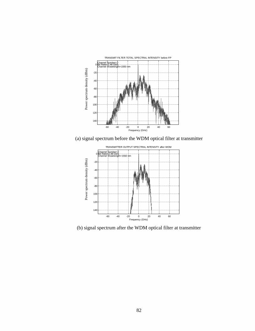
82

-60 -40 -20 0 20 40 60

-140

-120

-100

-80

-60

-40

-20

0

TRANSMIT FILTER TOTAL SPECTRAL INTENSITY before FP

Pul

se in

tens

ity (

mw

)

Frequency (GHz)

Channel Number=2 Bit Rate=2.48 Gb/sChannel Wavelength=1550 nm

(a) signal spectrum before the WDM optical filter at transmitter

-60 -40 -20 0 20 40 60

-140

-120

-100

-80

-60

-40

-20

0

TRANSMITTER OUTPUT SPECTRAL INTENSITY after WDM

Pul

se in

tens

ity (

mw

)

Frequency (GHz)

Channel Number=2 Bit Rate=2.48 Gb/sChannel Wavelength=1550 nm

(b) signal spectrum after the WDM optical filter at transmitter

Pow

er s

pect

rum

den

sity

(dB

m)

Pow

er s

pect

rum

den

sity

(dB

m)

83

-60 -40 -20 0 20 40 60

-140

-120

-100

-80

-60

-40

-20

0

this is the spectrum after attenuation and dispersion of fiber

Pul

se in

tens

ity (

mw

)

Frequency (GHz)

Channel Number=1 Bit Rate=2.48 Gb/sChannel Wavelength=1550 nm

(c) signal spectrum after the transmisssion over 70 km fiber

-80 -60 -40 -20 0 20 40 60 80-500

-450

-400

-350

-300

-250

-200

-150

-100output of the optical detector --> Overall Spectrum

(d) signal electrical spectrum after the photo detector

200 400 600 800 1000 1200 1400 1600 1800

0

0.05

0.1

0.15

0.2

0.25

0.3

RECEIVER ELECTRIC FILTER --> EYE DIAGRAM:

Pul

se in

tens

ity (

mW

)

Time (ps)

Channel Number=1 Channel Wavelength=1000000000 nmNumber of samples/bit=64

(e) eyediagram of subcarrier one after receiver baseband electrical filter

Pow

er s

pect

rum

den

sity

(dB

m)

Pow

er s

pect

rum

den

sity

(dB

m)

Puls

e am

plitu

de (

mA

)

Frequency (GHz)

84

200 400 600 800 1000 1200 1400 1600 1800

0

0.05

0.1

0.15

0.2

0.25

0.3

RECEIVER ELECTRIC FILTER --> EYE DIAGRAM:

Pul

se in

tens

ity (

mW

)

Time (ps)

Channel Number=2 Channel Wavelength=1000000000 nmNumber of samples/bit=64

(f) eyediagram of subcarrier two after receiver baseband electrical filter

Figure 3.6, signals for a QPSK system.

The OMI used to make these plots is 0.4. In order to find the impacts of OMI

and carrier suppression, we did simulations at different OMIs and carrier suppression

ratio similar to what we did in the BPSK systems. Figure 3.7 shows the receiver

sensitivity vs carrier suppression ratio at several different OMIs. The simulation were

performed for both back to back (figure 3.7(a) ) and after 300km SMF (figure 3.7 (b))

-2 5 -2 0 -1 5 -1 0 -5 0-3 4 .5

-3 4

-3 3 .5

-3 3

-3 2 .5

-3 2

-3 1 .5

-3 1

-3 0 .5

-3 0

(a) at 0kmCarrier suppression ratio (dB)

Sens

itivi

ty (

dBm

)

Puls

e am

plitu

de (

mA

)

OMI=0.1

OMI=0.2OMI=0.5

OMI=0.4OMI=0.3

85

-25 -20 -15 -10 -5 0-29

-28

-27

-26

-25

-24

-23

-22

(b) at 300km

Figure 3.7 QPSK system sensitivity as the function of OMI and carrier

suppression for different transmission distance

We found the carrier suppression in QPSK system has similar effect as in the

BPSK system. Since we tested 5dB carrier suppression in our experiment, we will

still use OMI of 0.3 and 5dB carrier suppression.

Table 3.2 summarizes the QPSK system results for different optical powers

levels. Please refer to the appendix 3 for the plots need to generate Tab. 3.2. In this

table, DC means dispersions compensation, OMI means optical modulation index, OP

means optical power, RFMI means RF modulation index, Freq 1 means the frequency

of lower subcarrier, L means longest transmission distance.

For the fiber with PMD parameter of 0.1ps/sqrt(km), the longest transmission

distance 1200 km can be achieved with 100% dispersion compensation and 3dBm

optical power. Decreasing optical power from 3dBm, the maximum transmission

distance will also be decreased. This is different from the situation of BPSK system,

where the nonlinearity is more severe and the system works better at smaller optical

power.

Carrier suppression ratio (dB)

Sens

itiv

ity

(dB

m)

OMI=0.1

OMI=0.2

OMI=0.5

OMI=0.4

OMI=0.3

86

For the fiber with PMD parameter of 0.5ps/sqrt(km), the longest transmission

distance is about 750 km with dispersion compensation and 5dBm optical power.

Since the highest subcarrier frequency is 11.2 GHz here which is smaller than 18

GHz used in BPSK system, the PMD walkoff problem is not as severe as in BPSK

system.

Without dispersion compensation, the transmission distance is 450 km no

matter what is the PMD parameter. Fiber nonlinearity is still one of the limiting factor

here.

PMD

kmps /

DC OMI OP(dBm) RFMI Freq1 L(km)

0.1 Yes 0.3 5 1 1 4 1100

0.1 Yes 0.4 5 1 1 4 950

0.1 Yes 0.3 3 1 1 4 1200

0.1 Yes 0.4 3 1 1 4 900

0.1 Yes 0.3 0 1 1 4 750

0.1 Yes 0.4 0 1 1 4 550

0.1 Yes 0.3 -3 1 1 4 500

0.1 Yes 0.4 -3 1 1 4 350

0.1 No 0.3 5 1 1 4 400

0.1 No 0.4 5 1 1 4 400

0.1 No 0.3 3 1 1 4 450

0.1 No 0.4 3 1 1 4 450

0.1 No 0.3 0 1 1 4 250

0.1 No 0.4 0 1 1 4 250

0.1 No 0.3 -3 1 1 4 250

0.1 No 0.4 -3 1 1 4 250

0.5 Yes 0.3 5 1 1 4 750

87

0.5 Yes 0.4 5 1 1 4 650

0.5 yes 0.3 3 1 1 4 700

0.5 yes 0.4 3 1 1 4 500

0.5 yes 0.3 0 1 1 4 500

0.5 yes 0.4 0 1 1 4 350

0.5 yes 0.3 -3 1 1 4 350

0.5 yes 0.4 -3 1 1 4 250

0.5 no 0.3 5 1 1 4 400

0.5 no 0.4 5 1 1 4 400

0.5 no 0.3 3 1 1 4 450

0.5 no 0.4 3 1 1 4 450

0.5 no 0.3 0 1 1 4 250

0.5 no 0.4 0 1 1 4 250

0.5 no 0.3 -3 1 1 4 250

0.5 no 0.4 -3 1 1 4 250

Table 3.2 longest transmission distance for BPSK SCM systems with different

parameters.

88

3.3 Performance of an SCM system with direct detection

In a 4 subcarriers BPSK system, the highest frequency subcarrier always

suffer from the effects of both polarization walk off and polarization mode dispersion.

The polarization effects severely limits the max transmission distance.

In order to reduce such undesired effect, we tried to reduce the highest signal

frequency by using QPSK modulation format. QPSK has a better PMD tolerance

compared to BPSK because the highest subcarrier frequency is reduced form about 17

GHz to 12 GHz. But it is still sensitive to the polarization limitation. One way to

overcome this problem is to use coherent detection for each of the subcarriers. This

method requires four very stable receiver lasers as the local oscillators, which is

obviously a very expensive solution. Another method is to use narrow band optical

filter to select the subcarrier directly in optical domains. This method is used in [1]

and the authors experimentally transmitted a 10 Gb/s signal through 4 subcarriers

each carrying 2.5 Gbps. A direct detection optical receiver was used using narrow

band optical filter to make cannel selection. The transmission distance reported was

490km and the sensitivity is about –25dBm. In this work [1] DSB was used. In

addition to its sensitivity to chromatic dispersion, the DSB modulation has 3dB

intrinsic system penalty due to its four unused subcarriers on the other side of the

carrier.

In such a system, the signal subcarrier is selected by optical filtering, so only

those modulation formats whose complex envelopes resemble their baseband signals

can be demodulated. This requirement implies the use of ASK as the modulation

format. Phase modulation format such as PSK or FSK will not give the desired

output. Also in the receiver an optical splitter is required to distribute the signal to

four different narrow band filters.

The narrow band optical filter we used in the simulation is a simple FP filter.

The reflectivity of the mirror is 0.99, which gives the finesse of the filter to be

312.5845. When the bandwidth of the passband is increased or decreased by changing

the spacing between the two mirrors, the free-spectral-range (FSR) will be increased

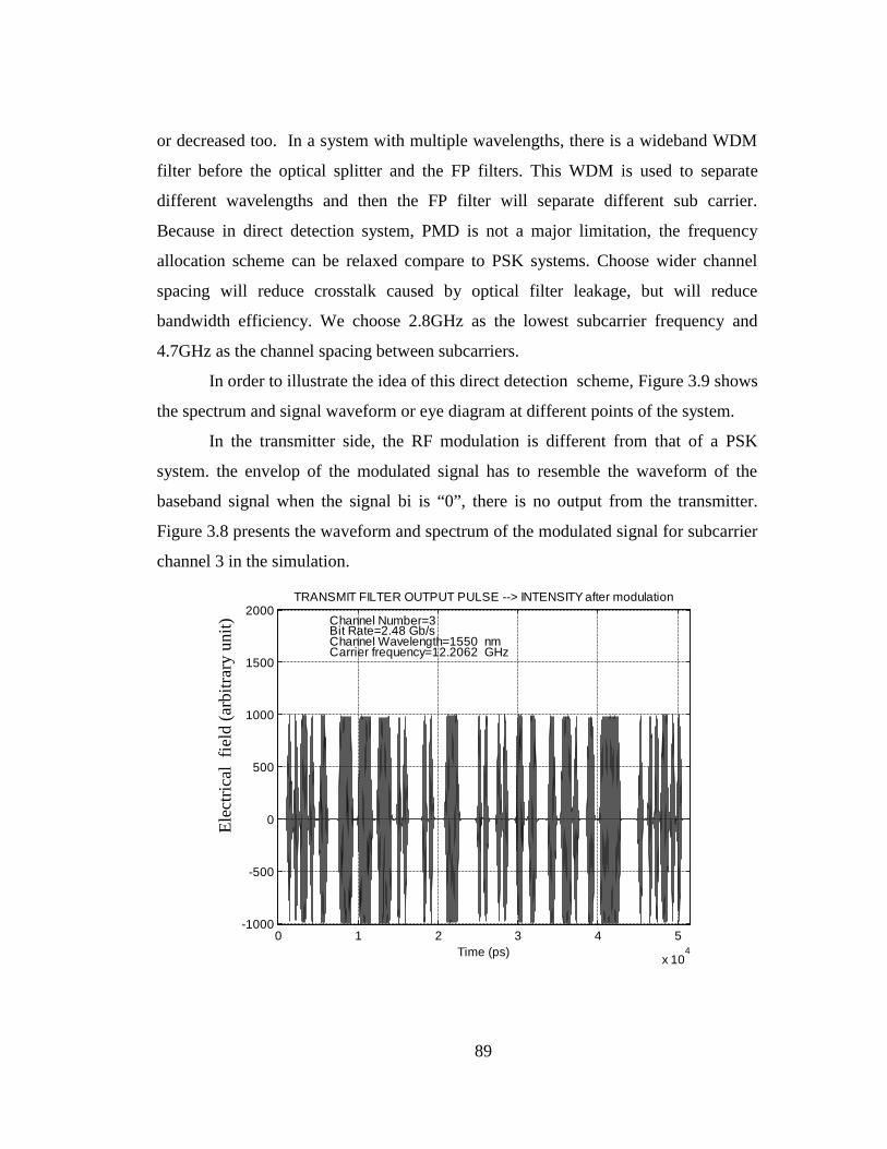
89

or decreased too. In a system with multiple wavelengths, there is a wideband WDM

filter before the optical splitter and the FP filters. This WDM is used to separate

different wavelengths and then the FP filter will separate different sub carrier.

Because in direct detection system, PMD is not a major limitation, the frequency

allocation scheme can be relaxed compare to PSK systems. Choose wider channel

spacing will reduce crosstalk caused by optical filter leakage, but will reduce

bandwidth efficiency. We choose 2.8GHz as the lowest subcarrier frequency and

4.7GHz as the channel spacing between subcarriers.

In order to illustrate the idea of this direct detection scheme, Figure 3.9 shows

the spectrum and signal waveform or eye diagram at different points of the system.

In the transmitter side, the RF modulation is different from that of a PSK

system. the envelop of the modulated signal has to resemble the waveform of the

baseband signal when the signal bi is “0”, there is no output from the transmitter.

Figure 3.8 presents the waveform and spectrum of the modulated signal for subcarrier

channel 3 in the simulation.

0 1 2 3 4 5

x 104

-1000

-500

0

500

1000

1500

2000TRANSMIT FILTER OUTPUT PULSE --> INTENSITY after modulation

Pul

se in

tens

ity (m

w)

Time (ps)

Channel Number=3 Bit Rate=2.48 Gb/sChannel Wavelength=1550 nmCarrier frequency=12.2062 GHz

Ele

ctri

cal

fiel

d (a

rbit

rary

uni

t)

90

-40 -30 -20 -10 0 10 20 30 40

-140

-120

-100

-80

-60

-40

-20

0

TRANSMIT FILTER OUTPUT PULSE --> SPECTRAL INTENSITY after modulation

Pul

se in

tens

ity (m

w)

Frequency (GHz)

Channel Number=3 Bit Rate=2.48 Gb/sChannel Wavelength=1550 nm

Figure 3.8 waveform and spectrum of the modulated signal for subcarrier 3

Figure 3.9 shows waveform and spectrum of the composite signal with

combined four subcarrier channels.

0 .5 1 1 .5 2 2 .5 3 3 .5 4 4 .5 5

x 1 04

-3 0 0 0

-2 0 0 0

-1 0 0 0

0

1 0 0 0

2 0 0 0

3 0 0 0

4 0 0 0

TRA NS M IT F IL TE R O UTP UT P UL S E --> IN TE NS ITY a fte r co m b ine r

Pul

se in

tens

ity (m

w)

T im e (p s)

(a)

Pow

er s

pect

rum

den

sity

(dB

)E

lect

rica

l fi

eld

(arb

itra

ry u

nit)

91

5 10 15 20 25 30-160

-140

-120

-100

-80

-60

-40

-20

0

TRANSMIT FILTER TOTAL SPECTRAL INTENSITY

Pul

se in

tens

ity (m

w)

Frequency (GHz)

(b)

Figure 3.9 waveform and spectrum of the composite signal

An important difference between the spectrums of the ASK and PSK

modulated signals is that ASK spectrum has a strong carrier component at each tone,

theis can be observed at Figure 3.9(b).

Figure 3.10 shows the waveform and spectrum of the optical signal with 4

subcarrier channels after the MZ optical modulator. The optical modulation index is

0.3.

Pow

er s

pect

rum

den

sity

(dB

)

92

0 1 2 3 4 5

x 104

0

1000

2000

3000

4000

5000

6000

7000

TRANSMIT FILTER OUTPUT PULSE --> INTENSITY before FP

Pul

se in

tens

ity (m

w)

Time (ps)

Channel Number=4 Bit Rate=2.48 Gb/sChannel Wavelength=1550 nmCarrier frequency=16.9144 GHz

-20 -10 0 10 20 30

-80

-70

-60

-50

-40

-30

-20

-10

0

TRA NS MIT F ILTE R TOTA L S P E C TRA L INTE NS ITY before F P

Pul

se in

tens

ity (m

w)

F requency (GHz)

Figure 3.10 spectrum and waveform of the modulated optical signal before

carrier suppression

The carrier component which is shown at 0 Hz has a very large amplitude and

is almost 25 dB higher than the subcarriers. If such a signal is transmitted, it will be

wasting a lot of optical power on the optical carrier and the modulation efficiency is

low. In addition, the lowest frequency subcarrier channel will be severely interfered

Am

plitu

de(d

B)

Puls

e in

tens

ity(

arbi

trar

y un

it)

Pow

er s

pect

rum

den

sity

(dB

)

93

by the strong carrier component. Avoiding this interference requires a very strong

frequency selectivity of the receiver optical filter. Therefore it is useful to suppress

the carrier component before it is sent out into the optical fiber.

The carrier suppression is done in the same way as we did in the PSK system.

Figure 3.11 shows the waveform and spectrum of the optical signal after 35 dB

carrier suppression.

0.5 1 1.5 2 2.5 3 3.5 4 4.5 5

x 104

0

50

100

150

200

250

300

350

400

450

500

TRA NS MIT F ILTE R OUTP UT P ULS E --> INTE NS ITY a fte r F P

Pul

se in

tens

ity (m

w)

Tim e (ps)

-2 0 -1 0 0 1 0 2 0 3 0

-6 0

-5 0

-4 0

-3 0

-2 0

-1 0

0

TR A N S M IT F IL TE R TO TA L S P E C TR A L IN TE N S ITY a fte r F P

Pul

se in

tens

ity (m

w)

F re q ue nc y (G H z)

Figure 3.11 spectrum and waveform of the modulated optical signal after

carrier suppression

Pow

er s

pect

rum

den

sity

(dB

)Pu

lse

inte

nsity

(arb

itrar

y un

it)

94

With the carrier suppression implemented, the carrier is almost 10 dB lower

than the sub carriers. In order to emphasize the modulation and demodulation

procedures, we first look at back-to-back signal performance without passing through

any optical fiber.

In the receiver side, the signal is first amplified by a wideband EDFA and then

a WDM demultiplexer to separate different wavelength channels. After the WDM

DEMUX, a star coupler or splitter has to be used to distribute the optical signal to

four narrow bandwidth FP filters each selecting a different subcarrier channel. We

should mention here that because the noise and signal has been attenuated by the

same amount, so it would not make difference in the sensitivity calculation whether

or not the optical filter attenuation is considered. Signal-ASE beat noise is always the

dominant noise in the simulation.

In the simulation, we varied the bandwidth of the FP filter by changing the

space between the two mirrors of the FP filter. The FSR will then be changed

accordingly.

In this particular case, the HPFW of the FP filter is 4GHz which is about 1.6

times the bit rate. Figure 3.12 shows the power and phase transfer function of the

filter.

-5 -4 -3 -2 -1 0 1 2 3 4

x 1 09

-3

-2 .5

-2

-1 .5

-1

-0 .5

0

F P fi lte r p o w e r a m p li tu d e tra n s fe r fu n c t i o n

Frequency (Hz)

Am

plitu

de (

dB)

95

- 8 -6 -4 -2 0 2 4 6 8

x 1 01 0

-2

-1 .5

-1

-0 .5

0

0 .5

1

1 .5

2F P f i lte r p h a s e tra n s fe r fu n c t i o n

Figure 3.12 Power and phase transfer function of a FP filter

Figure 3.13 is the spectrum and the waveform of the lowest frequency

subcarrier channel after the narrowband FP filter. The selectivity of the optical filter

is obviously not good. The selected subcarrier is only 10 dB higher than its adjacent

subcarrier.

-15 -10 -5 0 5 10 15 20-70

-60

-50

-40

-30

-20

-10

Frequency (GHz)

Pow

er S

pect

rum

Den

sity

(dB

m)

Figure 3.13, spectrum of the signal after the demuxing optical FP filter

Frequency (Hz)

Pha

se a

ngle

( R

adia

n)

96

Figure 3.14(a) shows electrical spectrum after the O/E conversion. The

selected signal power is only about 10 dB higher than the interference channels and

therefore the eyediagram has a lot of high frequency components as shown in Figure

3.14(b). The eye seems totally closed. Therefore an additional filtering is necessary to

remove high frequency interference.

-2 0 -1 5 -1 0 -5 0 5 1 0 1 5 2 0-1 0 0

-9 0

-8 0

-7 0

-6 0

-5 0

F re q u e n c y (G H z)

Pow

er S

pect

rum

Den

sity

(dB

m)

(a)

200 400 600 800 1000 1200 1400 1600 1800

0

0.1

0.2

0.3

0.4

0.5

eyediagram

Pul

se in

tens

ity (m

W)

Time (ps)

(b)

Figure 3.14, electrical spectrum and eyediagram after the photon diode

97

To this end we used a baseband electrical filter after the photodiode with

bandwidth of 0.7 times the bit rate. It effectively cleans up the eye diagram. Figure

3.15 shows the waveform ,eyediagram and spectrum of the signal after the baseband

electrical filter. The electrical filter used here is a 6 order butterworth filter.

0 .5 1 1 .5 2 2 .5 3 3 .5 4 4 .5 5

x 104

0

0 .05

0 .1

0 .15

0 .2

0 .25

0 .3

0 .35

0 .4

RE C E IV E R E LE C TRIC F ILTE R --> P ULS E INTE NS ITY:

Pul

se in

tens

ity (m

w)

Tim e (ps)

C hanne l Num ber=4 B it Ra te=2 .48 G b/sC hanne l W ave leng th=1000000000 nmC arrie r frequency=16 .9144 GHz

200 400 600 800 1000 1200 1400 1600 1800-0.1

-0.05

0

0.05

0.1

0.15

0.2

0.25

0.3

0.35

0.4 RECEIVER ELECTRIC FILTER --> EYE DIAGRAM:

Pul

se in

tens

ity (m

W)

Time (ps)

Channel Number=4 Channel Wavelength=1000000000 nmNumber of samples/bit=64

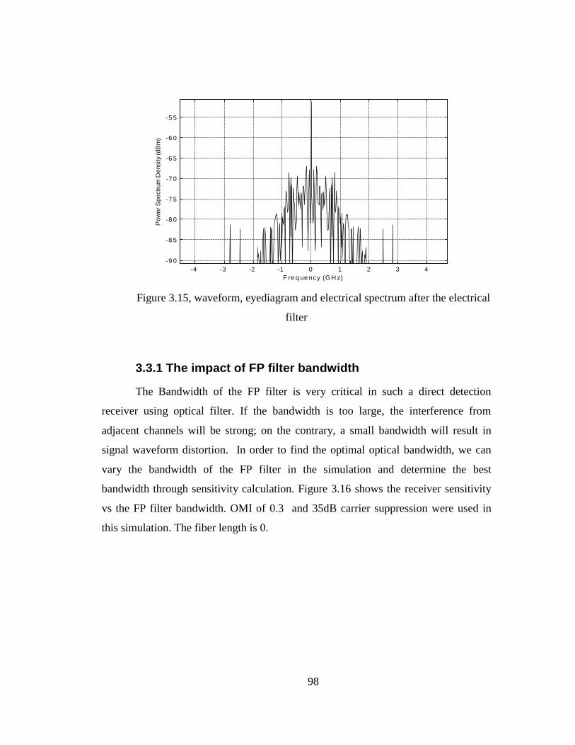
98

-4 -3 -2 -1 0 1 2 3 4-9 0

-8 5

-8 0

-7 5

-7 0

-6 5

-6 0

-5 5

F re q ue nc y (G H z)

Pow

er S

pect

rum

Den

sity

(dB

m)

Figure 3.15, waveform, eyediagram and electrical spectrum after the electrical

filter

3.3.1 The impact of FP filter bandwidth

The Bandwidth of the FP filter is very critical in such a direct detection

receiver using optical filter. If the bandwidth is too large, the interference from

adjacent channels will be strong; on the contrary, a small bandwidth will result in

signal waveform distortion. In order to find the optimal optical bandwidth, we can

vary the bandwidth of the FP filter in the simulation and determine the best

bandwidth through sensitivity calculation. Figure 3.16 shows the receiver sensitivity

vs the FP filter bandwidth. OMI of 0.3 and 35dB carrier suppression were used in

this simulation. The fiber length is 0.

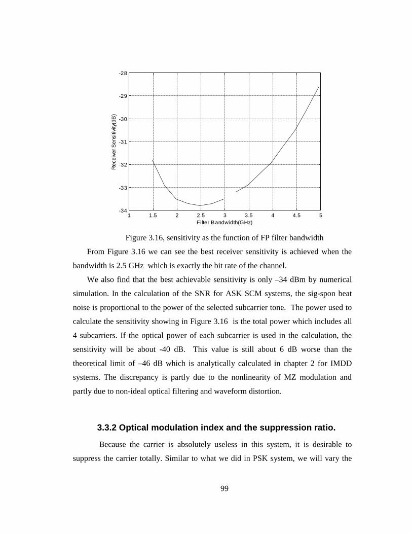
99

1 1.5 2 2.5 3 3.5 4 4.5 5-34

-33

-32

-31

-30

-29

-28

Rec

eive

r Sen

sitiv

ity(d

B)

Filter Bandwidth(GHz)

Figure 3.16, sensitivity as the function of FP filter bandwidth

From Figure 3.16 we can see the best receiver sensitivity is achieved when the

bandwidth is 2.5 GHz which is exactly the bit rate of the channel.

We also find that the best achievable sensitivity is only –34 dBm by numerical

simulation. In the calculation of the SNR for ASK SCM systems, the sig-spon beat

noise is proportional to the power of the selected subcarrier tone. The power used to

calculate the sensitivity showing in Figure 3.16 is the total power which includes all

4 subcarriers. If the optical power of each subcarrier is used in the calculation, the

sensitivity will be about -40 dB. This value is still about 6 dB worse than the

theoretical limit of –46 dB which is analytically calculated in chapter 2 for IMDD

systems. The discrepancy is partly due to the nonlinearity of MZ modulation and

partly due to non-ideal optical filtering and waveform distortion.

3.3.2 Optical modulation index and the suppression ratio.

Because the carrier is absolutely useless in this system, it is desirable to

suppress the carrier totally. Similar to what we did in PSK system, we will vary the

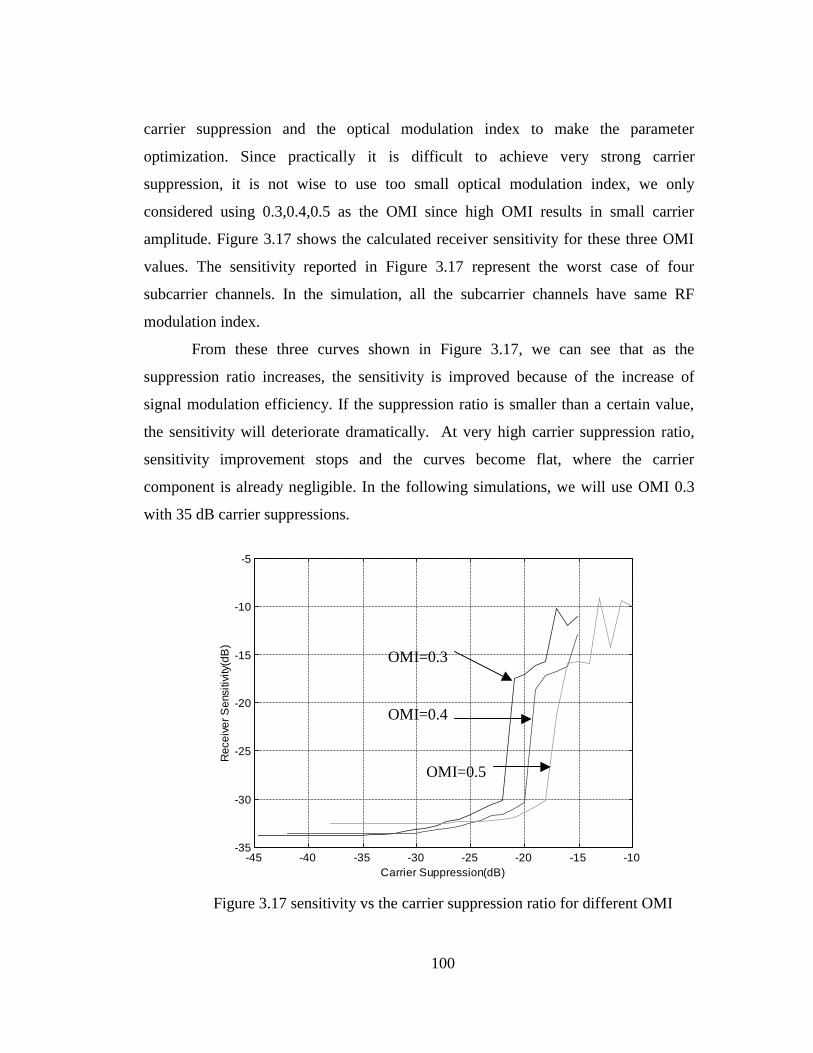
100

carrier suppression and the optical modulation index to make the parameter

optimization. Since practically it is difficult to achieve very strong carrier

suppression, it is not wise to use too small optical modulation index, we only

considered using 0.3,0.4,0.5 as the OMI since high OMI results in small carrier

amplitude. Figure 3.17 shows the calculated receiver sensitivity for these three OMI

values. The sensitivity reported in Figure 3.17 represent the worst case of four

subcarrier channels. In the simulation, all the subcarrier channels have same RF

modulation index.

From these three curves shown in Figure 3.17, we can see that as the

suppression ratio increases, the sensitivity is improved because of the increase of

signal modulation efficiency. If the suppression ratio is smaller than a certain value,

the sensitivity will deteriorate dramatically. At very high carrier suppression ratio,

sensitivity improvement stops and the curves become flat, where the carrier

component is already negligible. In the following simulations, we will use OMI 0.3

with 35 dB carrier suppressions.

-45 -40 -35 -30 -25 -20 -15 -10-35

-30

-25

-20

-15

-10

-5

Rec

eive

r Sen

sitiv

ity(d

B)

Carrier Suppression(dB)

Figure 3.17 sensitivity vs the carrier suppression ratio for different OMI

OMI=0.3

OMI=0.4

OMI=0.5

101

3.3.3 Effect of optical power

For back to back simulation, the system performance is independent of optical

power level because there is no optical fiber. When transmission fiber is introduced,

nonlinear effect of the fiber has to be considered and we have to decide the optical

power level to be used. We vary the optical power levels and run the simulation for

different fiber lengths. The optical powers we used are 5dBm, 3dBm, 0dBm, -3dBm,

Figure 3.18 shows the calculated receiver sensitivity versus fiber length at different

optical power levels:

0 200 400 600 800 1000 1200-35

-30

-25

-20

-15

-10

-5

0

5

10

Rec

eive

r Sen

sitiv

ity(d

B)

Fiber Length(km)

Figure 3.18 sensitivity curves with different optical power

It is obviously that system with optical power of 3dBm has the longest

transmission distance which is about 880km. 5dBm is worse than 3dBm because the

nonlinearity of the fiber becomes significant which causes waveform distortion of the

signal. –3dBm system can transmit less than 440km, that is because the signal noise

ratio at receiver is not large enough.

P=-3dBm

P=0dBm

P=3dBm

P=5dBm

102

3.3.4 four wavelength system results

In the last section, we have discussed the performance of single wavelength, 4

subcarrier SCM system using direct detection through an optical filter. Now we

extend our simulation into multi wavelengths. In a multi-wavelength system, the

interference both between wavelengths and between subcarriers in the same

wavelength channel have to be considered. Therefore additional performance

degradation may be introduced. Table 3.3 summarizes the major results of simulation

for a 4 wavelength ASK SCM system. Please see appendix 4 for the corresponding

plots.

Due to the nonlinear interference between wavelength channels, the optimum

optical power for a multiple wavelength WDM/SCM system is lower than that for a

single wavelength SCM system. From table 3.3, we found the dispersion

compensation does not help the system performance. This system is not dispersion

limited, instead, it is crosstalk noise limited. The longest transmission distance is

550km with 0dBm optical power and no dispersion compensation is used.

DC OMI OP(dBm) RFMI L(km)

Yes 0.3 3 1 1 1 1 50

Yes 0.3 0 1 1 1 1 200

Yes 0.3 -3 1 1 1 1 250

Yes 0.3 -6 1 1 1 1 250

No 0.3 3 1 1 1 1 250

No 0.3 0 1 1 1 1 550

no 0.3 -3 1 1 1 1 500

No 0.3 -6 1 1 1 1 350

Table 3.3 longest transmission distance for ASK SCM systems with different

parameters

103

3.4 system performance for a traditional four wavelength

OC192 system

In order to make comparison, we also did simulations on a traditional four

wavelengths ASK OC192 TDM system, the bit rate of each wavelength is 10Gbps.

NRZ modulation format was used in this simulation. The result presented here does

not consider the PMD effect.

As shown in table 3.4, without dispersion compensation, the transmission

distance of a 10Gb/s TDM system is limited to approximately 100km due to the high

bit rate. With dispersion compensation, the distance can be 1100 km with the optical

power per channel is 0dBm.

DC OMI OP(dBm) L(km)

Yes 0.5 3 950

Yes 0.5 0 1100

Yes 0.5 -3 800

Yes 0.5 -6 500

No 0.5 3 100

No 0.5 0 100

No 0.5 -3 100

No 0.5 -6 100

Table 3.4 longest transmission distance for traditional OC192 systems with

different parameters

104

Chapter Four

BPSK SCM system experiments

In the laboratory, a single-wavelength four-subcarrier BPSK SCM system

experiment was conducted. The experiment configuration is shown in figure 4.1.

3.6GHz

amplifier

Fiber

DetectorPre-amp

Pow

erco

mbi

n

Datagenerator

8.3GHz

17.5GHz

LPF

LPF

EDFAPre-amp.

Scope

13GHz

Pow

er S

plitt

er

2.488Gb/s

BERtester

LPF

LPF

3.6GHz

8.3GHz

13GHz

17.5GHz

Pow

er S

plitt

er

EDFAPost-amp

00

900

Laser

DC Bias

Figure.4.1, Basic configuration of an SCM/WDM optical system

In this setup, the 2.5Gb/s digital signal output from the BERT were split into 4

channels by a microwave power splitter. Then these four channels were delayed each

by a different time and then individually mixed with a microwave carrier at 3.6 GHz,

8.3 GHz, 13 GHz and 18 GHz respectively. They were then combined and amplified.

In order to generate optical single-side band signal, the amplified composite

RF signal was fed into a 90o hybrid splitter. One output of this splitter has a 90-degree

phase advance than the other output. This hybrid splitter has a frequency bandwidth

105

of 18GHz. The two outputs of the splitter were applied to the two arms of a dual

electrode LiNbO3 Mach-Zehnder modulator with 20 GHz bandwidth. A DC bias was

applied to one arm of the MZ modulator and set the modulator at the quadrature

operating point.

Figure 4.2 shows the SSB optical spectrum measured by a scanning Fabry-

Perot interferometer with 1GHz resolution bandwidth. The carrier is about 15 dB

higher than the subcarriers. And the subcarriers only appear on one side of the carrier.

The suppression is larger than 15 dB.

Figure 4.2 spectrum of generated OSSB signal by the MZ modulator

Then the optical signal is amplified by a post optical amplifier and launched

into a 75 km strand single mode fiber. At the receiver, the signal is amplified by an

EDFA preamplifier and then detected by a high-speed photo diode. The bandwidth of

the detector is larger than 20GHz. Figure 4.3 shows the electrical spectrum after O/E

conversion.

Nor

mal

ized

Opt

ical

spe

ctra

l den

sity

(dB

)

Frequency (GHz)-50 -40 -30 -20 -10 0 10 20 30 40

-35

-30

-25

-20

-15

-10

-5

0

106

The signal to noise ratio is larger than 20dB for the high frequency

subcarriers, but it is only 15dB for the low frequency subcarrier. This is similar to

what we saw in the simulation: lower frequency subcarriers are subject to more

distortion.

Figure 4.3, Detected composite signal RF spectrum

After photo detection, there is an electrical amplifier where signal is amplified

and then split by a power splitter into four ports. The output of each port is mixed

with four microwave carriers at 3.6 GHz, 8.3 GHz, 13 GHz and 18 GHz to perform

frequency down-conversion. The phase of the local oscillators are adjusted by RF

delay lines in order to get maximum signal outputs. Then the demodulated signal is

filtered by a 1.75GHz low pass filter. Fig. 4.4 gives an example of the demodulated

baseband spectrum.

-55

-50

-45

-40

-35

-30

-25

-20

0 2 4 6 8 10 12 14 16 18 20 22

Frequency (GHz)

Inte

nsit

y (d

Bm

)

107

Figure 4.4, electrical spectrum of a baseband signal after demodulation.

Fig. 4.5 shows eyediagrams of all the four-subcarrier channels for both back-

to-back (left column) and over 75km SMF (right column). All the eye diagrams were

measured at the bit-error rate of 10-10.

-85

-80

-75

-70

-65

-60

-55

-50

-45

0 1 2 3 4

F requenc y (G H z)

Inte

nsity

(dB

)

2.5Gb/s baseband spectrum at the

fc=8.3GHz, back-to-back, P=-23.5 dBm fc=8.3GHz, over fiber, P =-23 dBm

fc=3.6GHz, over fiber, P =-22.6 dBmfc=3.6GHz, back-to-back, P =-24.9 dBm

Inte

nsit

y(dB

m)

108

Figure 4.5, Measured eye diagrams of 3.6GHz, 8.3GHz, 13GHz and 17.5GHz

channels at the receiver for back/back (left column) and after 75km SMF transmission

(right column).

4.1 BER test

Bit error rate measurement was also performed for all four channels for both

back-to-back and over 75km standard SMF as shown in Figure 4.6. For back-to-back,

the sensitivity (for a BER of 10-9) ranges from –24dBm to –27dBm for different

channels mainly due to the ripples in the microwave devices. This value is about 4 to

7 dB less than we found with the simulation, this is mainly attributed to imperfect

devices and that the phase of the local oscillator may not be the optimum.

fc=13GHz, back-to-back, P =-27.6 dBm fc=13GHz, over fiber, P =-24 dBm

fc=17.5GHz, over fiber, P =-21.5 dBmfc=17.5GHz, back-to-back, P =-22.7 dBm

109

-34 -32 -30 -28 -26 -24 -2210-10

10-9

10-8

10-7

10-6

10-5

10-4

10-3Channel #1 (fc = 3.6GHz)

* back/backo over 75km SMF

-36 -34 -32 -30 -28 -26 -2410-10

10-9

10-8

10-7

10-6

10-5

10-4

10-3Channel #2 (fc = 8.3GHz)

* back/backo over 75km SMF

-36 -34 -32 -30 -28 -26 -2410-10

10-9

10-8

10-7

10-6

10-5

10-4

10-3Channel #3 (fc = 13GHz)

* back/backo over 75km SMF

-34 -32 -30 -28 -26 -24 -2210-10

10-9

10-8

10-7

10-6

10-5

10-4

10-3 Channel #4 (fc = 17.5GHz)

* back/backo over 75km SMF

BE

R

Optical power (dBm)

BE

R

BE

RB

ER

Optical power (dBm)

Optical power (dBm) Optical power (dBm)

Figure 4.6, Measured BER versus received optical power for all four channels both

back-to-back (stars) and over 75km SMF (circles).

After transmission of 75km of SMF, the sensitivity degraded by typically

2dB. The reason for this degradation is partly due to fiber nonlinearity and partly due

to the frequency instability of the local oscillators. In our experiment, the same RF

oscillators are shared by both the transmitter and the receiver (as local oscillators). A

fiber length of 75km corresponds to a time delay of approximately 0.38ms. Over this

time delay, the oscillators change their frequency (or phase) due to phase noise. This

caused a phase mismatch between RF carriers and local oscillators at the receiver and

thus resulted in measurable sensitivity degradations. However, in real commercial

systems, this problem can be solved by carrier recovery and phase-locked-loop.

110

Although special customer designs are generally required for the specific carrier

frequencies, both of these microwave techniques are commercially available.

4.2 Channel spacing

In order to pack all the four channels into a 20GHz modulator bandwidth, channel

spacing needs to be as narrow as possible. Since each channel carries a 2.5Gb/s

traffic, its double side electrical bandwidth is approximately 1.75*2 = 3.5GHz

(information bandwidth). Figure 4.7 shows the receiver sensitivity versus channel

spacing for a 2 subcarriers system. The minimum channel spacing is found to be

about 4.7GHz in our experiment. Below this limit, significant sensitivity degradation

cased by inter-channel crosstalk is observed. This minimum channel spacing largely

depends on the quality of the baseband filter. A sharp cut off outside the passband is

desired to reduce the inter-channel crosstalk and to reduce channel spacing. The

reason why this experimentally determined minimum channel spacing number is

larger than we got from the simulation is because in the simulation, the electrical

filter was ideal which has a sharp cut off outside the passband.

Figure 4.7, Impact of channel spacing on the receiver sensitivity

-35

-34

-33

-32

-31

-30

-29

-28

-27

-26

4.4 4.6 4.8 5 5.2 5.4 5.6 5.8

FR channel separation (GHz)

Rec

eive

r se

nsit

ivit

y (d

Bm

)

111

4.3 Carrier suppression

We also investigated the effect of optical carrier suppression experimentally.

Fig.4.8 shows the experimental set-up for carrier suppression. A fabry-Perot

Interferometer (FPI) was used as a wavelength dependent reflector and an optical

circulator was used to re-direct the optical signal. The wavelength of the FPI was

tuned by its electrical bias in order to obtain an appropriate amount of carrier

suppression.

As discussed in the chapter 2, receiver sensitivity can be improved by optical

carrier suppression approximately on a dB per dB base. Fig.4.9 shows a measured

BER plot to demonstrate the effect of carrier suppression. This was performed in a

single channel system with the carrier suppression of approximately 5dB. Clearly the

receiver sensitivity was improved by approximately 3dB in this case.

Figure 4.8, Experimental set-up for optical carrier suppression.

Output

LD

Mach-ZehnderModulator

CW

Signal

CirculatorFabry-Perotfilter

Fine Tuning

112

Figure 4.9, Comparison of system performance with and without optical

suppression.

The effect of modulation index on the sensitivity improvement due to carrier

suppression is demonstrated in Figure 4.10. As the RF power increases, the sensitivity

improvement due to carrier suppression is decreased. This is exactly what we saw in

the simulation.

Figure 4.10, Effect of modulation index on the sensitivity improvement due to

a 7 dB carrier suppression.

-41 -40 -39 -38 -37 -36 -35 -34 -33 -32 -31 -30

Received Power (dBm)

-12

-11

-10

-9

-8

-7

-6

-5

-4

-3

-2

Log

(BER)

back-to-back

optical carriersuppressed

-39

-37

-35

-33

-31

-29

0 2 4 6 8RF power to modulator (dBm)

Rec

eive

d se

nsiti

vity

(dB

m)

no carrier suppression

with carrier suppression

Log

(BE

R)

Received power(dBm)

113

4.4 Comparison between SCM and TDM at OC192 Rates

With standard SMF, chromatic dispersion alone limits the transmission distance of

an uncompensated OC192 system to approximately 100km. On the other hand, the

dispersion limited transmission distance for an OC48 system is typically 500km with

standard SMF. For the reason of comparison, we did a OC192 sensitivity

measurement with variable system accumulated dispersion. In the following Fig.

4.11, the curve with solid squares represents the sensitivity of an OC192 system and

the curve with triangles represents the sensitivity of a 4-channel OC48 BPSK SCM

system.

Figure 4.11, sensitivity of traditional OC192 and a 4 channels OC48 BPSK

SCM system vs the accumulated dispersion

Due to the limitation of fiber availability, the experiment was performed with

negative dispersion DC fibers (dispersion compensating fiber), which have large

dispersion values. Assume that the dispersion value for a standard SMF is

17ps/nm/km, we can convert the accumulated dispersion in the experimental system

-35

-30

-25

-20

-15

-10

-5

SMF Equivalent Fiber Length (km)

Rec

eive

r se

nsit

ivit

y (d

Bm

)

TDM

SCM

0 20 40 60 80 100 120 140 160 180 200

340 680 1020 1360 1700 2040 2380 2720 3060 34000

Accumulated dispersion (ps/nm)

114

into an equivalent length of standard SMF. At back-to-back, the sensitivity of the

SCM system is about 6dB worse compared to its TDM counterpart. With the

accumulated dispersion of higher than 1700ps/nm (corresponds to 100km of SMF),

the performance of the TDM system deteriorates rapidly with the increase of the

dispersion, while the performance of the SCM system remains unchanged.

Because of the limitation of the fiber availability in the laboratory, we only

measured the system with the equivalent SMF length of up to 150km.

Although dispersion induced distortion penalty in TDM systems can be reduced by

dispersion compensation, however, attenuation of dispersion compensating module is

typically 6 to 8dB for each 80km equivalent SMF span. This attenuation adds to the

system link budget. In addition, dispersion compensation increases the cost of system

equipment and system design engineering and thus makes systems less flexible.

115

Chapter FiveConclusion and future work

In conclusion, we have studied some possible applications of subcarrier

multiplexing and optical-single-side-band modulation in transporting high-speed data

through standard single mode fiber. The targeted data speed per wavelength is

10Gbps or OC192 speed. Three different types of optical SCM system were

simulated and the results are presented by sensitivity and eye opening vs transmission

distance. These three types of SCM systems are: 4-subcarrier BPSK SCM system, 2-

subcarrier QPSK SCM system, 4-subcarrier ASK SCM system. They all have 4

wavelengths with 10Gbps capacity on each wavelength. The wavelength spacing is

50GHz.

In order to obtain these sensitivity values, for each setup, parameters’

optimization are had to be done for optical modulation index, carrier suppression

ratio, RF modulation index, channel spacing, frequency allocation, electrical filter

bandwidth, and optical filter bandwidth.

We demonstrated that optical carrier suppression is an effective way to

improve the receiver sensitivity when the modulation index is relatively low and it

can improve system performance by reducing the nonlinearity of the modulation

process.

We discussed the impact of PMD effect and considered 2 effects: PMD-

induced polarization walkoff and PMD-induced waveform distortion. We considered

the first effect in our simulation and estimated the second effect, analytically.

We simulated the system performance for different optical power levels in

order to find the optimal optical power range for each system configuration. We

selected two different PMD coefficients of optical fibers and investigated the compact

of dispersion compensation. Table 5.1 below gives the transmission distance limit for

each type of system.

116

System type Dispersion

Compensation

PMD

coefficient

kmps /

Distance

limit

(km)

Power range

(dBm)

BPSK SCM DC 0.1 450 5dBm

BPSK SCM No DC 0.1 350 0 to 3dBm

BPSK SCM DC 0.5 350 3 to 5dBm

BPSK SCM No DC 0.5 300 0 dBm

QPSK SCM DC 0.1 1200 3 to 5 dBm

QPSK SCM No DC 0.1 450 3 dBm

QPSK SCM DC 0.5 750 3 to 5 dBm

QPSK SCM No DC 0.5 450 3 to 5 dBm

ASK SCM DC 0.1 250 -3 to –6dBm

ASK SCM No DC 0.1 550 -3 to 0dBm

OC192 DC 0.1 1100 0 dBm

OC192 No DC 0.1 100 -6 to 3dBm

Table 5.1, Transmission distance limit for different type of systems

From the simulation, BPSK system is most suitable for applications within

300 to 350 km with no dispersion compensation. QPSK system is suitable for

application up to 750 km with dispersion compensation and 450 without dispersion

compensation. ASK system is not recommended because the maximum distance is

only 550 km while the narrow band optical fiber is very difficult to implement and

stabilize.

In addition to numerical simulations, we have demonstrated a four-channel

digital SCM system with the aggregated capacity of 10Gb/s. Compare to TDM

OC192 systems, this SCM system is less sensitive to chromatic dispersion. Also it is

more flexible in terms of channel add/drop.

Through this extensive study, we believe that to upgrade optical systems from

OC48 rate to OC192, sub-carrier multiplexing is feasible and practical. SCM has

117

several advantages over TDM as mentioned above, especially in systems with

standard single mode fibers.

Future work

Recently, some WDM system vendors are starting to use a channels spacing

of 6.25 GHz for OC48 channel and they are using Raman amplification to reduce the

noise and optical power and thus reduced the nonlinearities. From the simulation

results, we found that when optical power is small, the SCM system would not incur

much distortion even after long distance transmission. It is only limited by ASE

noise. So SCM system also can be used with Raman amplification and with a small

optical power. It can reduce the number of optical sources in the system. It would be

interesting to see the system performance with Raman amplification.

Multilevel signal such as QAM could be used to further increase the spectrum

efficiency. Microwave single sideband modulation could also be used for this

purpose. And it is very likely that they will have good application in short distance

applications.

The PMD effect is only estimated in this study. Detailed analysis of PMD

effect is necessary and it should be implemented into the simulation in order to get

more accurate result.

From the simulation, we found single wavelength SCM system has much

better performance than a same type four wavelengths SCM system. We need setup

up a multi-wavelength SCM test bed in the laboratory and verify it experimentally.

Experimental investigation of QPSK and M-ary SCM may also be necessary.

118

References

1. Paul D. Sargis etc. 10Gb/s subcarrier multiplexed transmission over 490km of

ordinary single mode fiber without dispersion compensation., IEEE PTL, Dec,1997

2. Anthony P. Foord etc, Optical demultiplexing for subcarrier multiplexed systems,

IEEE Transactions on Microwave theory and techniques. 2324-2329,1995,9

3. P.M. Hill etc. ,8 Gb/s subcarrier multiplexed coherent lightwave system, IEEE PTL,

Aug,1991

4. Bandwidth efficient transmission of 4Gb/s on two microwave QPSK subcarriers over

a 48 km optical link, IEEE PTL, july, 1990

5. P.D. Sargis etc. Dispersion reduction technique using subcarrier multiplexing. Proc.

SPIE. Oct. 1995. Vol. 2614, pp 244-251

6. Subcarrier multiplexing with dispersion reduction and direct detection. EL, Sept. 28,

1995

7. Javier Marti etc, modeling optically prefiltered AM Subcarrier Multiplexed systems,

IEEE Transactions on Microwave theory and techniques. 2249-2256,1993,9

8. Anthony P. Foord, optical demultiplexing for subcarrier multiplexed system, IEEE

Transactions on Microwave theory and techniques. 2324-2329,1995,9

9. Mike Sieben, Jan Conradi, Optical single sideband transmission at 10 Gb/s using only

electrical dispersion compensation. JLT, OCT. 1999

10. Moshe Nazarathy, etc. Progress in externally modulated AM CATV transmission

systems, JLT, Jan. 1993

11. M.R. Phillips etc. Nonlinear distortion generated by dispersive transmission of

chirped intensity modulated signals PTL, May, 1991

12. M.C. Wu etc. CSO distortions due to the combined effects of self and external phase

modulation, OFC 96, TuP1-1

13. Sen Lin Zhang etc. Assessment of the nonlinearity tolerance of different modulation

schemes for millimeter wave fiber radio systems using MZ modulators, IEEE

Transactions on Microwave theory and techniques. Aug, 1997

14. G. P. Agrawal, Nonlinear Fiber optics. New York: Academic, 1995

15. G. P. Agrawal, Fiber communication systems. John wiley &sons, 1997

119

16. L.W. Couch II, Digital and analog communication systems, Prentice Hall, 1997

17. Michel C. Jeruchim etc. Simulation of communication systems.

18. P. Kaminow etc. optical fiber telecommunications. IIIA, Academic, 1997

19. F.S.Yang etc., Nonlinear crosstalk and SBS reduction by carrier suppression in SCM-

WDM optical communication system, OFC99

1

Appendix 1

Some considerations for the simulation of

communications system

Low pass equivalent signals and systems

The signal in this simulation is represented by the complex envelope of the

real signal. Below is some explanation.

Computer simulation of communications signal and systems are always being

done in the sampled or digital domain. Because a continuous signal is uniquely

represented by a discrete model only if that the sampling frequency is at least twice

the highest frequency in the signal spectrum. So Because the optical frequency is so

high, you can not sample the signal directly, even for one bit of signal of a OC48

channel, direct sampling will generate more than 7.7e4 samples, you have to find a

equivalent way to simulate the signal with much less sampling rate,

One technique is the so-called complex envelope method, which makes use of

the concepts of low pass equivalent signals and systems.

For any carrier modulated signal )(tx , if the signal bandwidth is much less

than the carrier frequency, we can write

])(Re[)( )( tjtj ceetrtx ωφ= , here )(tr is the amplitude modulation and ( )tφ is the

phase modulation of the signal. And cω is the carrier frequency

)()( tjetr φ contains all of the information related variations and has low pass

nature. It is often called the complex envelope or complex low pass equivalent of the

signal. For optical signal, the bandwidth of the signal is always much less than the

carrier frequency and thus can be written into this format.

For a LTI (linear time invariant) system, the system output for an input )(tx is

2

)()()( thtxty ∗= , )(th is the impulse response of the system. It can be proved that we

also have )()(2

1)( thtxty LLL ∗= , the suffix L represent the low pass equivalent

signal. And we have ])(Re[)( tjL

cetyty ω=

This is to say that the processing and transmission of the bandpass signal can

be evaluated through its low pass envelope. So the whole simulation can be done with

this complex envelope if the system is LTI. In our program, we represent the

microwave signal with its directly sampled signal. When it is goes to the optical

domain, we will use complex envelope for that optical signal. the transform is done at

the optical modulator and detector.

Power relationship of complex envelope and the real signal

Because we use complex envelope in the simulation, we have to know the

power relationship of complex envelope and the real signal. it is very important for

the calculation of the sensitivity.

For a passband signal )sin()()cos()()( φωφω +−+= ttyttxts cc . Its time

averaged power is )]([2

1)]([

2

1 22 tyAvgtxAvg + . The complex signal of the signal is

)()()( tjytxtz += , time averaged power in the envelope is )]()([ 22 tytxAvg + and it

is two times the power of the real passband signal. In the simulation , you should be

very careful about this.

Power spectrum (PSD) estimation

If a random process is ergodic, it can be shown that its PSD can be defined in

terms of a time average as

∑−=∞>−

−+

=M

MnM

xx fndTjnxdTdTM

EfS |)2exp()(|)12(

1lim)( 2π

3

If we eliminate the limiting operation by assuming a finite data set of N

samples for )(nx and eliminates the expectation operation by restricting our attention

to a single sample function, it becomes ∑−

=

−=1

0

2|)2exp()(|)(N

nxx fndTjnx

N

dTfS π .

If we let f ->k, dT->1/N, then we have

22

1

0

22

|))((|1

|)/2exp()(|1

)( nxfftN

NknjnxN

kSN

nxx =−= ∑

−

=

π .

Estimating the sampling rate for nonlinear systems

The SCM system is not a strict linear system. The optical fiber and the photon

detector are not linear at all. We should know that the spectrum of the output of a

nonlinear system does not generally have the same frequency components as the

input. The processing of a band-limited baseband signal by a nonlinear system will

increases the bandwidth greatly.

If we expand the output into a power series, it is easy to show if the input is

limited to the bandwidth B , the output is limited to Bn * , n is the highest order in the

series

In practical, we don’t have to use Bn * because the small coefficient of those

high order terms, another reason is a phenomenon called self concentration which

means the resulted spectrum will concentrated around the input spectrum in most

nonlinear system. But some increase in sampling rate will be required to keep the

aliasing error at an acceptably low level.

Filtering: Butterworth and Bessel filter

Bessel filters are a class of all pole filters that are characterized by the system

function )(/1)( sBsH N= , where )(sBN is the N th-order Bessel polynomial. These

polynomials can be expressed in the form.

4

∑=

=N

k

kkN sasB

0

)( , where the coefficients ka are given as

)!(!2

)!2(

kNk

kNa

kNk −−= − , Nk ,....,1,0= ,

alternatively the Bessel polynomials may be generated recursively form the

relation )()()12()( 22

1 sBssBNsB NNN −− +−= , with 1)(0 =sB and 1)(1 += ssB as

initial conditions.

You have to find the 3 dB frequency first and then translate the filter into your

desired frequency.

An important characteristic of Bessel filters is the linear phase response over

the passband of the filter.

The expression of Butterworth filter is mdBfffH *2

3 )/(1/1)( += . m is the

order of the Butterworth filter, f3db is the 3 dB bandwidth of the filter. Butterworth

filter usually have a narrower transition bandwidth compared to the Bessel filter

1

Appendix 2 : BPSK SCM results

In the titles of following plots, DC means 100% dispersion compensation, CS

means subcarriers suppression, the parameters from left to right are dispersion

compensation, PMD coefficient, optical power of each wavelength, frequency of first

subcarrier, optical modulation index and carrier suppression ratio. In appendix 3,4

and 5 , we will use the same abbreviation.

1. DC, 0.1 kmps / PMD, 5dBm, 2.6GHz, 0.3 and 5 dB CS

0 100 200 300 400 500 600 700 800 900 1000-35

-30

-25

-20

-15

-10

-5

0

5

10

Fiber Length (km)

Sen

sitiv

ity (dB

m)

sensitivity vs fiber length

WDM channel1 of 1WDM channel frequency:0optical modulation index:0.3optical power:5 dBmRF modulation index:1 1 1 1carrier suppression:-5.0327 dB2.615625e+009PMD Coefficiency:0.1 ps/sqrt(km)DC factor:100%

0 200 400 600 800 1000 1200

-30

-20

-10

0

10

Fiber Length (km)

Sen

sitiv

ity (dB

m)

0.3 -5.0327dBsc (0.9 0.9 1.15 1.35) 2.6156GHz 4.6888GHz 5dBm

0 200 400 600 800 1000 1200

-30

-20

-10

0

10

Fiber Length (km)

Sen

sitiv

ity (dB

m)

0.1ps/sqrt(km) 100%compensated 49.9681GHz 450km, chan1

0 200 400 600 800 1000 1200

-30

-20

-10

0

10

Fiber Length (km)

Sen

sitiv

ity (dB

m)

0 200 400 600 800 1000 1200

-30

-20

-10

0

10

Fiber Length (km)

Sen

sitiv

ity (dB

m)

0 200 400 600 800 1000 12000

0.5

1

x 10-4

Fiber Length (km)

Eye

Ope

n

0 200 400 600 800 1000 12000

0.5

1

x 10-4

Fiber Length (km)

Eye

Ope

n

0 200 400 600 800 1000 12000

0.5

1

x 10-4

Fiber Length (km)

Eye

Ope

n

0 200 400 600 800 1000 12000

0.5

1

x 10-4

Fiber Length (km)

Eye

Ope

n

2

2. DC, 0.1 kmps / PMD, 5dBm, 2.6GHz, 0.4 and 0 dB CS

0 100 200 300 400 500 600 700 800 900 1000-35

-30

-25

-20

-15

-10

-5

0

5

10

Fiber Length (km)

Sen

sitiv

ity (

dBm

)

sensitivity vs fiber length

WDM channel1 of 1WDM channel frequency:0optical modulation index:0.4optical power:5 dBmRF modulation index:1 1 1 1carrier suppression:0 dB2.615625e+009PMD Coefficiency:0.1 ps/sqrt(km)DC factor:100%

0 200 400 600 800 1000 1200

-30

-20

-10

0

10

Fiber Length (km)

Sen

sitiv

ity (dB

m)

0.4 0dBsc (0.9 0.9 1.15 1.35) 2.6156GHz 4.6888GHz 5dBm

0 200 400 600 800 1000 1200

-30

-20

-10

0

10

Fiber Length (km)

Sen

sitiv

ity (dB

m)

0.1ps/sqrt(km) 100%compensated 49.9681GHz 300km, chan3

0 200 400 600 800 1000 1200

-30

-20

-10

0

10

Fiber Length (km)

Sen

sitiv

ity (dB

m)

0 200 400 600 800 1000 1200

-30

-20

-10

0

10

Fiber Length (km)

Sen

sitiv

ity (dB

m)

0 200 400 600 800 1000 12000

0.5

1

x 10-4

Fiber Length (km)

Eye

Ope

n

0 200 400 600 800 1000 12000

0.5

1

x 10-4

Fiber Length (km)

Eye

Ope

n

0 200 400 600 800 1000 12000

0.5

1

x 10-4

Fiber Length (km)

Eye

Ope

n

0 200 400 600 800 1000 12000

0.5

1

x 10-4

Fiber Length (km)

Eye

Ope

n

3

3. DC, 0.1 kmps / PMD, 3dBm, 2.6GHz, 0.3 and 5 dB CS

0 100 200 300 400 500 600 700 800 900 1000-35

-30

-25

-20

-15

-10

-5

0

5

10

Fiber Length (km)

Sen

sitiv

ity (

dBm

)sensitivity vs fiber length

WDM channel1 of 1WDM channel frequency:0optical modulation index:0.3optical power:3.0001 dBmRF modulation index:1 1 1 1carrier suppression:-5.0327 dB2.615625e+009PMD Coefficiency:0.1 ps/sqrt(km)DC factor:100%

0 200 400 600 800 1000 1200

-30

-20

-10

0

10

Fiber Length (km)

Sen

sitiv

ity (dB

m)

0.3 -5.0327dBsc (0.9 0.9 1.15 1.35) 2.6156GHz 4.6888GHz 3dBm

0 200 400 600 800 1000 1200

-30

-20

-10

0

10

Fiber Length (km)

Sen

sitiv

ity (dB

m)

0.1ps/sqrt(km) 100%compensated 49.9681GHz 350km, chan2

0 200 400 600 800 1000 1200

-30

-20

-10

0

10

Fiber Length (km)

Sen

sitiv

ity (dB

m)

0 200 400 600 800 1000 1200

-30

-20

-10

0

10

Fiber Length (km)

Sen

sitiv

ity (dB

m)

0 200 400 600 800 1000 12000

0.5

1

x 10-4

Fiber Length (km)

Eye

Ope

n

0 200 400 600 800 1000 12000

0.5

1

x 10-4

Fiber Length (km)

Eye

Ope

n

0 200 400 600 800 1000 12000

0.5

1

x 10-4

Fiber Length (km)

Eye

Ope

n

0 200 400 600 800 1000 12000

0.5

1

x 10-4

Fiber Length (km)

Eye

Ope

n

4

4. DC, 4. 0.1 kmps / PMD, 3dBm, 2.6GHz, 0.4 and 0 dB CS

0 100 200 300 400 500 600 700 800 900 1000-35

-30

-25

-20

-15

-10

-5

0

5

10

Fiber Length (km)

Sen

sitiv

ity (

dBm

)

sensitivity vs fiber lengthWDM channel1 of 1WDM channel frequency:0optical modulation index:0.4optical power:3.0001 dBmRF modulation index:1 1 1 1carrier suppression:0 dB2.615625e+009PMD Coefficiency:0.1 ps/sqrt(km)DC factor:100%

0 200 400 600 800 1000 1200

-30

-20

-10

0

10

Fiber Length (km)

Sen

sitiv

ity (dB

m)

0.4 0dBsc (0.9 0.9 1.15 1.35) 2.6156GHz 4.6888GHz 3dBm

0 200 400 600 800 1000 1200

-30

-20

-10

0

10

Fiber Length (km)

Sen

sitiv

ity (dB

m)

0.1ps/sqrt(km) 100%compensated 49.9681GHz 400km, chan1

0 200 400 600 800 1000 1200

-30

-20

-10

0

10

Fiber Length (km)

Sen

sitiv

ity (dB

m)

0 200 400 600 800 1000 1200

-30

-20

-10

0

10

Fiber Length (km)

Sen

sitiv

ity (dB

m)

0 200 400 600 800 1000 12000

0.5

1

x 10-4

Fiber Length (km)

Eye

Ope

n

0 200 400 600 800 1000 12000

0.5

1

x 10-4

Fiber Length (km)

Eye

Ope

n

0 200 400 600 800 1000 12000

0.5

1

x 10-4

Fiber Length (km)

Eye

Ope

n

0 200 400 600 800 1000 12000

0.5

1

x 10-4

Fiber Length (km)

Eye

Ope

n

5

5. DC, 0.1 kmps / PMD, 0dBm, 2.6GHz, 0.3 and 5 dB CS

0 200 400 600 800 1000 1200-30

-20

-10

0

10

Fiber Length (km)

Sen

sitiv

ity (

dBm

)

0.3 -5.0327dBsc (0.9 0.9 1.15 1.35) 2.6156GHz 4.6888GHz 0dBm

0 200 400 600 800 1000 1200-30

-20

-10

0

10

Fiber Length (km)

Sen

sitiv

ity (

dBm

)

0.1ps/sqrt(km) 100%compensated 49.9681GHz 350km, chan1

0 200 400 600 800 1000 1200-30

-20

-10

0

10

Fiber Length (km)

Sen

sitiv

ity (

dBm

)

0 200 400 600 800 1000 1200-30

-20

-10

0

10

Fiber Length (km)

Sen

sitiv

ity (

dBm

)

0 200 400 600 800 1000 12000

0.5

1

x 10-4

Fiber Length (km)

Eye

Ope

n

0 200 400 600 800 1000 12000

0.5

1

x 10-4

Fiber Length (km)

Eye

Ope

n0 200 400 600 800 1000 1200

0

0.5

1

x 10-4

Fiber Length (km)

Eye

Ope

n

0 200 400 600 800 1000 12000

0.5

1

x 10-4

Fiber Length (km)

Eye

Ope

n

6

6. No DC, 0.1 kmps / PMD, 5dBm, 2.6GHz, 0.3 and 5 dB CS

0 100 200 300 400 500 600 700 800-35

-30

-25

-20

-15

-10

-5

0

5

Fiber Length (km)

Sen

sitiv

ity (d

Bm

)sensitivity vs fiber length

WDM channel1 of 1WDM channel frequency is0optical modulation index is0.3optical power is5 dBmRF modulation index is1 1 1 1carrier suppression is-5.0327 dB2.615625e+009

RF chan 1RF chan 2RF chan 3RF chan 4

0 200 400 600 800 1000 1200

-30

-20

-10

0

10

Fiber Length (km)

Sen

sitiv

ity (

dBm

)

0.3 -5.0327dBsc (1.12 1.05 1.05 0.9) 2.6156GHz 4.6888GHz 5dBm

0 200 400 600 800 1000 1200

-30

-20

-10

0

10

Fiber Length (km)

Sen

sitiv

ity (

dBm

)

0.1ps/sqrt(km) 0%compensated 49.9681GHz 200.0001km, chan2

0 200 400 600 800 1000 1200

-30

-20

-10

0

10

Fiber Length (km)

Sen

sitiv

ity (

dBm

)

0 200 400 600 800 1000 1200

-30

-20

-10

0

10

Fiber Length (km)

Sen

sitiv

ity (

dBm

)

0 200 400 600 800 1000 12000

0.5

1

x 10-4

Fiber Length (km)

Eye

Ope

n

0 200 400 600 800 1000 12000

0.5

1

x 10-4

Fiber Length (km)

Eye

Ope

n

0 200 400 600 800 1000 12000

0.5

1

x 10-4

Fiber Length (km)

Eye

Ope

n

0 200 400 600 800 1000 12000

0.5

1

x 10-4

Fiber Length (km)

Eye

Ope

n

7

7. DC, 0.1 kmps / PMD, 0dBm, 2.6GHz, 0.4 and 0 dB CS

0 200 400 600 800 1000 1200

-30

-20

-10

0

10

Fiber Length (km)

Sen

sitiv

ity (dB

m)

0.4 0dBsc (0.9 0.9 1.15 1.35) 2.6156GHz 4.6888GHz 0dBm

0 200 400 600 800 1000 1200

-30

-20

-10

0

10

Fiber Length (km)

Sen

sitiv

ity (dB

m)

0.1ps/sqrt(km) 100%compensated 49.9681GHz 250km, chan1

0 200 400 600 800 1000 1200

-30

-20

-10

0

10

Fiber Length (km)

Sen

sitiv

ity (dB

m)

0 200 400 600 800 1000 1200

-30

-20

-10

0

10

Fiber Length (km)

Sen

sitiv

ity (dB

m)

0 200 400 600 800 1000 12000

0.5

1

x 10-4

Fiber Length (km)

Eye

Ope

n

0 200 400 600 800 1000 12000

0.5

1

x 10-4

Fiber Length (km)

Eye

Ope

n0 200 400 600 800 1000 1200

0

0.5

1

x 10-4

Fiber Length (km)

Eye

Ope

n

0 200 400 600 800 1000 12000

0.5

1

x 10-4

Fiber Length (km)E

ye O

pen

8. DC, 0.1 kmps / PMD, -3dBm, 2.6GHz, 0.3 and -5 dB CS

0 200 400 600 800 1000 1200

-30

-20

-10

0

10

Fiber Length (km)

Sen

sitiv

ity (dB

m)

0.3 -5.0327dBsc (0.9 0.9 1.15 1.35) 2.6156GHz 4.6888GHz -3.0001dBm

0 200 400 600 800 1000 1200

-30

-20

-10

0

10

Fiber Length (km)

Sen

sitiv

ity (dB

m)

0.1ps/sqrt(km) 100%compensated 49.9681GHz 250km, chan1

0 200 400 600 800 1000 1200

-30

-20

-10

0

10

Fiber Length (km)

Sen

sitiv

ity (dB

m)

0 200 400 600 800 1000 1200

-30

-20

-10

0

10

Fiber Length (km)

Sen

sitiv

ity (dB

m)

0 200 400 600 800 1000 12000

0.5

1

x 10-4

Fiber Length (km)

Eye

Ope

n

0 200 400 600 800 1000 12000

0.5

1

x 10-4

Fiber Length (km)

Eye

Ope

n

0 200 400 600 800 1000 12000

0.5

1

x 10-4

Fiber Length (km)

Eye

Ope

n

0 200 400 600 800 1000 12000

0.5

1

x 10-4

Fiber Length (km)

Eye

Ope

n

8

9. DC, 0.1 kmps / PMD, -3dBm, 2.6GHz, 0.4 and 0 dB CS

0 200 400 600 800 1000 1200

-30

-20

-10

0

10

Fiber Length (km)

Sen

sitiv

ity (dB

m)

0.4 0dBsc (0.9 0.9 1.15 1.35) 2.6156GHz 4.6888GHz -3.0001dBm

0 200 400 600 800 1000 1200

-30

-20

-10

0

10

Fiber Length (km)

Sen

sitiv

ity (dB

m)

0.1ps/sqrt(km) 100%compensated 49.9681GHz 200.0001km, chan3

0 200 400 600 800 1000 1200

-30

-20

-10

0

10

Fiber Length (km)

Sen

sitiv

ity (dB

m)

0 200 400 600 800 1000 1200

-30

-20

-10

0

10

Fiber Length (km)

Sen

sitiv

ity (dB

m)

0 200 400 600 800 1000 12000

0.5

1

x 10-4

Fiber Length (km)

Eye

Ope

n

0 200 400 600 800 1000 12000

0.5

1

x 10-4

Fiber Length (km)

Eye

Ope

n0 200 400 600 800 1000 1200

0

0.5

1

x 10-4

Fiber Length (km)

Eye

Ope

n

0 200 400 600 800 1000 12000

0.5

1

x 10-4

Fiber Length (km)E

ye O

pen

9

10. No DC, 0.1 kmps / PMD, 5dBm, 2.6GHz, 0.4 and 0 dB CS

0 100 200 300 400 500 600 700 800-35

-30

-25

-20

-15

-10

-5

0

5

Fiber Length (km)

Sen

sitiv

ity (d

Bm

)sensitivity vs fiber length

WDM channel1 of 1WDM channel frequency is0optical modulation index is0.4optical power is5 dBmRF modulation index is1 1 1 1carrier suppression is0 dB2.615625e+009

RF chan 1RF chan 2RF chan 3RF chan 4

0 200 400 600 800 1000 1200

-30

-20

-10

0

10

Fiber Length (km)

Sen

sitiv

ity (dB

m)

0.4 0dBsc (1.12 1.05 1.05 0.9) 2.6156GHz 4.6888GHz 5dBm

0 200 400 600 800 1000 1200

-30

-20

-10

0

10

Fiber Length (km)

Sen

sitiv

ity (dB

m)

0.1ps/sqrt(km) 0%compensated 49.9681GHz 200.0001km, chan2

0 200 400 600 800 1000 1200

-30

-20

-10

0

10

Fiber Length (km)

Sen

sitiv

ity (

dBm

)

0 200 400 600 800 1000 1200

-30

-20

-10

0

10

Fiber Length (km)

Sen

sitiv

ity (

dBm

)

0 200 400 600 800 1000 12000

0.5

1

x 10-4

Fiber Length (km)

Eye

Ope

n

0 200 400 600 800 1000 12000

0.5

1

x 10-4

Fiber Length (km)

Eye

Ope

n

0 200 400 600 800 1000 12000

0.5

1

x 10-4

Fiber Length (km)

Eye

Ope

n

0 200 400 600 800 1000 12000

0.5

1

x 10-4

Fiber Length (km)

Eye

Ope

n

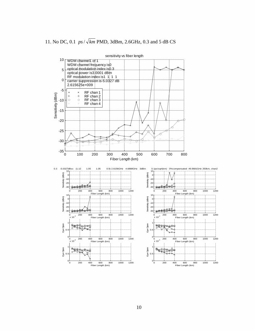
10

11. No DC, 0.1 kmps / PMD, 3dBm, 2.6GHz, 0.3 and 5 dB CS

0 100 200 300 400 500 600 700 800-35

-30

-25

-20

-15

-10

-5

0

5

10

Fiber Length (km)

Sen

sitiv

ity (d

Bm

)sensitivity vs fiber length

WDM channel1 of 1WDM channel frequency is0optical modulation index is0.3optical power is3.0001 dBmRF modulation index is1 1 1 1carrier suppression is-5.0327 dB2.615625e+009

RF chan 1RF chan 2RF chan 3RF chan 4

0 200 400 600 800 1000 1200

-30

-20

-10

0

10

Fiber Length (km)

Sen

sitiv

ity (dB

m)

0.3 -5.0327dBsc (1.12 1.05 1.05 0.9) 2.6156GHz 4.6888GHz 3dBm

0 200 400 600 800 1000 1200

-30

-20

-10

0

10

Fiber Length (km)

Sen

sitiv

ity (dB

m)

0.1ps/sqrt(km) 0%compensated 49.9681GHz 250km, chan2

0 200 400 600 800 1000 1200

-30

-20

-10

0

10

Fiber Length (km)

Sen

sitiv

ity (dB

m)

0 200 400 600 800 1000 1200

-30

-20

-10

0

10

Fiber Length (km)

Sen

sitiv

ity (dB

m)

0 200 400 600 800 1000 12000

0.5

1

x 10-4

Fiber Length (km)

Eye

Ope

n

0 200 400 600 800 1000 12000

0.5

1

x 10-4

Fiber Length (km)

Eye

Ope

n

0 200 400 600 800 1000 12000

0.5

1

x 10-4

Fiber Length (km)

Eye

Ope

n

0 200 400 600 800 1000 12000

0.5

1

x 10-4

Fiber Length (km)

Eye

Ope

n

11

12. No DC, 0.1 kmps / PMD, 3dBm, 2.6GHz, 0.4 and 0 dB CS

0 100 200 300 400 500 600 700 800-35

-30

-25

-20

-15

-10

-5

0

5

10

Fiber Length (km)

Sen

sitiv

ity (d

Bm

)sensitivity vs fiber length

WDM channel1 of 1WDM channel frequency is0optical modulation index is0.4optical power is3.0001 dBmRF modulation index is1 1 1 1carrier suppression is0 dB2.615625e+009

RF chan 1RF chan 2RF chan 3RF chan 4

0 200 400 600 800 1000 1200

-30

-20

-10

0

10

Fiber Length (km)

Sen

sitiv

ity (dB

m)

0.4 0dBsc (1.12 1.05 1.05 0.9) 2.6156GHz 4.6888GHz 3dBm

0 200 400 600 800 1000 1200

-30

-20

-10

0

10

Fiber Length (km)

Sen

sitiv

ity (dB

m)

0.1ps/sqrt(km) 0%compensated 49.9681GHz 250km, chan2

0 200 400 600 800 1000 1200

-30

-20

-10

0

10

Fiber Length (km)

Sen

sitiv

ity (dB

m)

0 200 400 600 800 1000 1200

-30

-20

-10

0

10

Fiber Length (km)

Sen

sitiv

ity (dB

m)

0 200 400 600 800 1000 12000

0.5

1

x 10-4

Fiber Length (km)

Eye

Ope

n

0 200 400 600 800 1000 12000

0.5

1

x 10-4

Fiber Length (km)

Eye

Ope

n

0 200 400 600 800 1000 12000

0.5

1

x 10-4

Fiber Length (km)

Eye

Ope

n

0 200 400 600 800 1000 12000

0.5

1

x 10-4

Fiber Length (km)

Eye

Ope

n

12

13. No DC, 0.1 kmps / PMD, 0dBm, 2.6GHz, 0.3 and 5 dB CS

0 200 400 600 800 1000 1200-30

-20

-10

0

10

Fiber Length (km)

Sen

sitiv

ity (dB

m)

0.3 -5.0327dBsc (1.12 1.05 1.05 0.9) 2.6156GHz 4.6888GHz 0dBm

0 200 400 600 800 1000 1200-30

-20

-10

0

10

Fiber Length (km)

Sen

sitiv

ity (dB

m)

0.1ps/sqrt(km) 0%compensated 49.9681GHz 350km, chan2

0 200 400 600 800 1000 1200-30

-20

-10

0

10

Fiber Length (km)

Sen

sitiv

ity (dB

m)

0 200 400 600 800 1000 1200-30

-20

-10

0

10

Fiber Length (km)

Sen

sitiv

ity (dB

m)

0 200 400 600 800 1000 12000

0.5

1

x 10-4

Fiber Length (km)

Eye

Ope

n

0 200 400 600 800 1000 12000

0.5

1

x 10-4

Fiber Length (km)

Eye

Ope

n

0 200 400 600 800 1000 12000

0.5

1

x 10-4

Fiber Length (km)

Eye

Ope

n

0 200 400 600 800 1000 12000

0.5

1

x 10-4

Fiber Length (km)

Eye

Ope

n

14. No DC, 0.1 kmps / PMD, 0dBm, 2.6GHz, 0.4 and 0 dB CS

0 200 400 600 800 1000 1200-30

-20

-10

0

10

Fiber Length (km)

Sen

sitiv

ity (dB

m)

0.4 0dBsc (1.12 1.05 1.05 0.9) 2.6156GHz 4.6888GHz 0dBm

0 200 400 600 800 1000 1200-30

-20

-10

0

10

Fiber Length (km)

Sen

sitiv

ity (dB

m)

0.1ps/sqrt(km) 0%compensated 49.9681GHz 350km, chan1

0 200 400 600 800 1000 1200-30

-20

-10

0

10

Fiber Length (km)

Sen

sitiv

ity (dB

m)

0 200 400 600 800 1000 1200-30

-20

-10

0

10

Fiber Length (km)

Sen

sitiv

ity (dB

m)

0 200 400 600 800 1000 12000

0.5

1

x 10-4

Fiber Length (km)

Eye

Ope

n

0 200 400 600 800 1000 12000

0.5

1

x 10-4

Fiber Length (km)

Eye

Ope

n

0 200 400 600 800 1000 12000

0.5

1

x 10-4

Fiber Length (km)

Eye

Ope

n

0 200 400 600 800 1000 12000

0.5

1

x 10-4

Fiber Length (km)

Eye

Ope

n

13

15. No DC, 0.1 kmps / PMD, -3dBm, 2.6GHz, 0.3 and 5 dB CS

0 200 400 600 800 1000 1200-30

-20

-10

0

10

Fiber Length (km)

Sen

sitiv

ity (dB

m)

0.3 -5.0327dBsc (1.12 1.05 1.05 0.9) 2.6156GHz 4.6888GHz -3.0001dBm

0 200 400 600 800 1000 1200-30

-20

-10

0

10

Fiber Length (km)

Sen

sitiv

ity (dB

m)

0.1ps/sqrt(km) 0%compensated 49.9681GHz 350km, chan1

0 200 400 600 800 1000 1200-30

-20

-10

0

10

Fiber Length (km)

Sen

sitiv

ity (

dBm

)

0 200 400 600 800 1000 1200-30

-20

-10

0

10

Fiber Length (km)

Sen

sitiv

ity (

dBm

)

0 200 400 600 800 1000 12000

0.5

1

x 10-4

Fiber Length (km)

Eye

Ope

n

0 200 400 600 800 1000 12000

0.5

1

x 10-4

Fiber Length (km)

Eye

Ope

n

0 200 400 600 800 1000 12000

0.5

1

x 10-4

Fiber Length (km)

Eye

Ope

n

0 200 400 600 800 1000 12000

0.5

1

x 10-4

Fiber Length (km)

Eye

Ope

n

16. No DC, 0.1 kmps / PMD, -3dBm, 2.6GHz, 0.4 and 0 dB CS

0 200 400 600 800 1000 1200-30

-20

-10

0

10

Fiber Length (km)

Sen

sitiv

ity (dB

m)

0.4 0dBsc (1.12 1.05 1.05 0.9) 2.6156GHz 4.6888GHz -3.0001dBm

0 200 400 600 800 1000 1200-30

-20

-10

0

10

Fiber Length (km)

Sen

sitiv

ity (dB

m)

0.1ps/sqrt(km) 0%compensated 49.9681GHz 250km, chan2

0 200 400 600 800 1000 1200-30

-20

-10

0

10

Fiber Length (km)

Sen

sitiv

ity (dB

m)

0 200 400 600 800 1000 1200-30

-20

-10

0

10

Fiber Length (km)

Sen

sitiv

ity (dB

m)

0 200 400 600 800 1000 12000

0.5

1

x 10-4

Fiber Length (km)

Eye

Ope

n

0 200 400 600 800 1000 12000

0.5

1

x 10-4

Fiber Length (km)

Eye

Ope

n

0 200 400 600 800 1000 12000

0.5

1

x 10-4

Fiber Length (km)

Eye

Ope

n

0 200 400 600 800 1000 12000

0.5

1

x 10-4

Fiber Length (km)

Eye

Ope

n

14

17. DC, 0.5 kmps / PMD, 5dBm, 2.6GHz, 0.3 and 5 dB CS

0 100 200 300 400 500 600 700 800 900 1000-35

-30

-25

-20

-15

-10

-5

0

5

10

Fiber Length (km)

Sen

sitiv

ity (

dBm

)sensitivity vs fiber length

WDM channel1 of 1WDM channel frequency:0optical modulation index:0.3optical power:5 dBmRF modulation index:1 1 1 1carrier suppression:-5.0327 dB2.615625e+009PMD Coefficiency:0.5 ps/sqrt(km)DC factor:100%

0 200 400 600 800 1000 1200

-30

-20

-10

0

10

Fiber Length (km)

Sen

sitiv

ity (

dBm

)

0.3 -5.0327dBsc (0.9 0.9 1.15 1.35) 2.6156GHz 4.6888GHz 5dBm

0 200 400 600 800 1000 1200

-30

-20

-10

0

10

Fiber Length (km)

Sen

sitiv

ity (

dBm

)

0.5ps/sqrt(km) 100%compensated 49.9681GHz 350km, chan1

0 200 400 600 800 1000 1200

-30

-20

-10

0

10

Fiber Length (km)

Sen

sitiv

ity (

dBm

)

0 200 400 600 800 1000 1200

-30

-20

-10

0

10

Fiber Length (km)

Sen

sitiv

ity (

dBm

)

0 200 400 600 800 1000 12000

0.5

1

x 10-4

Fiber Length (km)

Eye

Ope

n

0 200 400 600 800 1000 12000

0.5

1

x 10-4

Fiber Length (km)

Eye

Ope

n

0 200 400 600 800 1000 12000

0.5

1

x 10-4

Fiber Length (km)

Eye

Ope

n

0 200 400 600 800 1000 12000

0.5

1

x 10-4

Fiber Length (km)

Eye

Ope

n

15

18. DC, 0.5 kmps / PMD, 5dBm, 2.6GHz, 0.4 and 0 dB CS

0 100 200 300 400 500 600 700 800 900 1000-35

-30

-25

-20

-15

-10

-5

0

5

10

Fiber Length (km)

Sen

sitiv

ity (dB

m)

sensitivity vs fiber length

WDM channel1 of 1WDM channel frequency:0optical modulation index:0.4optical power:5 dBmRF modulation index:1 1 1 1carrier suppression:0 dB2.615625e+009PMD Coefficiency:0.5 ps/sqrt(km)DC factor:100%

0 200 400 600 800 1000 1200

-30

-20

-10

0

10

Fiber Length (km)

Sen

sitiv

ity (dB

m)

0.4 0dBsc (0.9 0.9 1.15 1.35) 2.6156GHz 4.6888GHz 5dBm

0 200 400 600 800 1000 1200

-30

-20

-10

0

10

Fiber Length (km)

Sen

sitiv

ity (dB

m)

0.5ps/sqrt(km) 100%compensated 49.9681GHz 350km, chan1

0 200 400 600 800 1000 1200

-30

-20

-10

0

10

Fiber Length (km)

Sen

sitiv

ity (dB

m)

0 200 400 600 800 1000 1200

-30

-20

-10

0

10

Fiber Length (km)

Sen

sitiv

ity (dB

m)

0 200 400 600 800 1000 12000

0.5

1

x 10-4

Fiber Length (km)

Eye

Ope

n

0 200 400 600 800 1000 12000

0.5

1

x 10-4

Fiber Length (km)

Eye

Ope

n

0 200 400 600 800 1000 12000

0.5

1

x 10-4

Fiber Length (km)

Eye

Ope

n

0 200 400 600 800 1000 12000

0.5

1

x 10-4

Fiber Length (km)

Eye

Ope

n

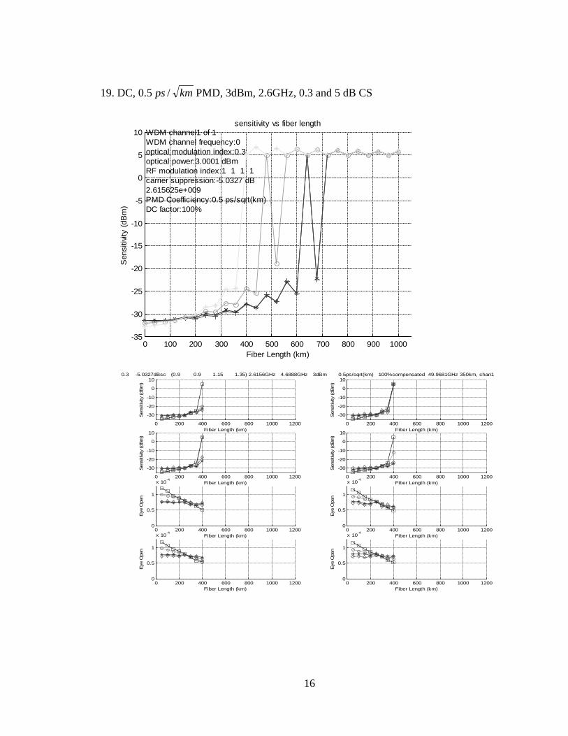
16

19. DC, 0.5 kmps / PMD, 3dBm, 2.6GHz, 0.3 and 5 dB CS

0 100 200 300 400 500 600 700 800 900 1000-35

-30

-25

-20

-15

-10

-5

0

5

10

Fiber Length (km)

Sen

sitiv

ity (

dBm

)sensitivity vs fiber length

WDM channel1 of 1WDM channel frequency:0optical modulation index:0.3optical power:3.0001 dBmRF modulation index:1 1 1 1carrier suppression:-5.0327 dB2.615625e+009PMD Coefficiency:0.5 ps/sqrt(km)DC factor:100%

0 200 400 600 800 1000 1200

-30

-20

-10

0

10

Fiber Length (km)

Sen

sitiv

ity (dB

m)

0.3 -5.0327dBsc (0.9 0.9 1.15 1.35) 2.6156GHz 4.6888GHz 3dBm

0 200 400 600 800 1000 1200

-30

-20

-10

0

10

Fiber Length (km)

Sen

sitiv

ity (dB

m)

0.5ps/sqrt(km) 100%compensated 49.9681GHz 350km, chan1

0 200 400 600 800 1000 1200

-30

-20

-10

0

10

Fiber Length (km)

Sen

sitiv

ity (dB

m)

0 200 400 600 800 1000 1200

-30

-20

-10

0

10

Fiber Length (km)

Sen

sitiv

ity (dB

m)

0 200 400 600 800 1000 12000

0.5

1

x 10-4

Fiber Length (km)

Eye

Ope

n

0 200 400 600 800 1000 12000

0.5

1

x 10-4

Fiber Length (km)

Eye

Ope

n

0 200 400 600 800 1000 12000

0.5

1

x 10-4

Fiber Length (km)

Eye

Ope

n

0 200 400 600 800 1000 12000

0.5

1

x 10-4

Fiber Length (km)

Eye

Ope

n

17

20. DC, 0.5 kmps / PMD, 3dBm, 2.6GHz, 0.4 and 0 dB CS

0 100 200 300 400 500 600 700 800 900 1000-35

-30

-25

-20

-15

-10

-5

0

5

10

Fiber Length (km)

Sen

sitiv

ity (

dBm

)sensitivity vs fiber length

WDM channel1 of 1WDM channel frequency:0optical modulation index:0.4optical power:3.0001 dBmRF modulation index:1 1 1 1carrier suppression:0 dB2.615625e+009PMD Coefficiency:0.5 ps/sqrt(km)DC factor:100%

0 200 400 600 800 1000 1200

-30

-20

-10

0

10

Fiber Length (km)

Sen

sitiv

ity (dB

m)

0.4 0dBsc (0.9 0.9 1.15 1.35) 2.6156GHz 4.6888GHz 3dBm

0 200 400 600 800 1000 1200

-30

-20

-10

0

10

Fiber Length (km)

Sen

sitiv

ity (dB

m)

0.5ps/sqrt(km) 100%compensated 49.9681GHz 350km, chan1

0 200 400 600 800 1000 1200

-30

-20

-10

0

10

Fiber Length (km)

Sen

sitiv

ity (dB

m)

0 200 400 600 800 1000 1200

-30

-20

-10

0

10

Fiber Length (km)

Sen

sitiv

ity (dB

m)

0 200 400 600 800 1000 12000

0.5

1

x 10-4

Fiber Length (km)

Eye

Ope

n

0 200 400 600 800 1000 12000

0.5

1

x 10-4

Fiber Length (km)

Eye

Ope

n

0 200 400 600 800 1000 12000

0.5

1

x 10-4

Fiber Length (km)

Eye

Ope

n

0 200 400 600 800 1000 12000

0.5

1

x 10-4

Fiber Length (km)

Eye

Ope

n

18

21. DC, 0.5 kmps / PMD, 0dBm, 2.6GHz, 0.3 and 5 dB CS

0 200 400 600 800 1000 1200-30

-20

-10

0

10

Fiber Length (km)

Sen

sitiv

ity (dB

m)

0.3 -5.0327dBsc (0.9 0.9 1.15 1.35) 2.6156GHz 4.6888GHz 0dBm

0 200 400 600 800 1000 1200-30

-20

-10

0

10

Fiber Length (km)

Sen

sitiv

ity (dB

m)

0.5ps/sqrt(km) 100%compensated 49.9681GHz 250km, chan2

0 200 400 600 800 1000 1200-30

-20

-10

0

10

Fiber Length (km)

Sen

sitiv

ity (dB

m)

0 200 400 600 800 1000 1200-30

-20

-10

0

10

Fiber Length (km)

Sen

sitiv

ity (dB

m)

0 200 400 600 800 1000 12000

0.5

1

x 10-4

Fiber Length (km)

Eye

Ope

n

0 200 400 600 800 1000 12000

0.5

1

x 10-4

Fiber Length (km)

Eye

Ope

n

0 200 400 600 800 1000 12000

0.5

1

x 10-4

Fiber Length (km)

Eye

Ope

n

0 200 400 600 800 1000 12000

0.5

1

x 10-4

Fiber Length (km)

Eye

Ope

n

22. DC, 0.5 kmps / PMD, 0dBm, 2.6GHz, 0.4 and 0 dB CS

0 200 400 600 800 1000 1200-30

-20

-10

0

10

Fiber Length (km)

Sen

sitiv

ity (dB

m)

0.4 0dBsc (0.9 0.9 1.15 1.35) 2.6156GHz 4.6888GHz 0dBm

0 200 400 600 800 1000 1200-30

-20

-10

0

10

Fiber Length (km)

Sen

sitiv

ity (dB

m)

0.5ps/sqrt(km) 100%compensated 49.9681GHz 250km, chan1

0 200 400 600 800 1000 1200-30

-20

-10

0

10

Fiber Length (km)

Sen

sitiv

ity (dB

m)

0 200 400 600 800 1000 1200-30

-20

-10

0

10

Fiber Length (km)

Sen

sitiv

ity (dB

m)

0 200 400 600 800 1000 12000

0.5

1

x 10-4

Fiber Length (km)

Eye

Ope

n

0 200 400 600 800 1000 12000

0.5

1

x 10-4

Fiber Length (km)

Eye

Ope

n

0 200 400 600 800 1000 12000

0.5

1

x 10-4

Fiber Length (km)

Eye

Ope

n

0 200 400 600 800 1000 12000

0.5

1

x 10-4

Fiber Length (km)

Eye

Ope

n

19

23. DC, 0.5 kmps / PMD, -3dBm, 2.6GHz, 0.3 and 5 dB CS

0 200 400 600 800 1000 1200-30

-20

-10

0

10

Fiber Length (km)

Sen

sitiv

ity (dB

m)

0.3 -5.0327dBsc (0.9 0.9 1.15 1.35) 2.6156GHz 4.6888GHz -3.0001dBm

0 200 400 600 800 1000 1200-30

-20

-10

0

10

Fiber Length (km)

Sen

sitiv

ity (dB

m)

0.5ps/sqrt(km) 100%compensated 49.9681GHz 250km, chan1

0 200 400 600 800 1000 1200-30

-20

-10

0

10

Fiber Length (km)

Sen

sitiv

ity (dB

m)

0 200 400 600 800 1000 1200-30

-20

-10

0

10

Fiber Length (km)

Sen

sitiv

ity (dB

m)

0 200 400 600 800 1000 12000

0.5

1

x 10-4

Fiber Length (km)

Eye

Ope

n

0 200 400 600 800 1000 12000

0.5

1

x 10-4

Fiber Length (km)

Eye

Ope

n

0 200 400 600 800 1000 12000

0.5

1

x 10-4

Fiber Length (km)

Eye

Ope

n

0 200 400 600 800 1000 12000

0.5

1

x 10-4

Fiber Length (km)

Eye

Ope

n

24. DC, 0.5 kmps / PMD, -3dBm, 2.6GHz, 0.4 and 0 dB CS

0 200 400 600 800 1000 1200-30

-20

-10

0

10

Fiber Length (km)

Sen

sitiv

ity (dB

m)

0.4 0dBsc (0.9 0.9 1.15 1.35) 2.6156GHz 4.6888GHz -3.0001dBm

0 200 400 600 800 1000 1200-30

-20

-10

0

10

Fiber Length (km)

Sen

sitiv

ity (dB

m)

0.5ps/sqrt(km) 100%compensated 49.9681GHz 150km, chan3

0 200 400 600 800 1000 1200-30

-20

-10

0

10

Fiber Length (km)

Sen

sitiv

ity (dB

m)

0 200 400 600 800 1000 1200-30

-20

-10

0

10

Fiber Length (km)

Sen

sitiv

ity (dB

m)

0 200 400 600 800 1000 12000

0.5

1

x 10-4

Fiber Length (km)

Eye

Ope

n

0 200 400 600 800 1000 12000

0.5

1

x 10-4

Fiber Length (km)

Eye

Ope

n

0 200 400 600 800 1000 12000

0.5

1

x 10-4

Fiber Length (km)

Eye

Ope

n

0 200 400 600 800 1000 12000

0.5

1

x 10-4

Fiber Length (km)

Eye

Ope

n

20

25. No DC, 0.5 kmps / PMD, 5dBm, 2.6GHz, 0.3 and 5 dB CS

0 100 200 300 400 500 600-35

-30

-25

-20

-15

-10

-5

0

5

10

Fiber Length (km)

Sen

sitiv

ity (d

Bm

)

sensitivity vs fiber lengthWDM channel1 of 1WDM channel frequency:0optical modulation index:0.3optical power:5 dBmRF modulation index:1 1 1 1carrier suppression:-5.0327 dB2.615625e+009PMD Coefficiency:0.5 ps/sqrt(km)DC factor:0%

0 200 400 600 800 1000 1200

-30

-20

-10

0

10

Fiber Length (km)

Sen

sitiv

ity (dB

m)

0.3 -5.0327dBsc (1.12 1.05 1.05 0.9) 2.6156GHz 4.6888GHz 5dBm

0 200 400 600 800 1000 1200

-30

-20

-10

0

10

Fiber Length (km)

Sen

sitiv

ity (dB

m)

0.5ps/sqrt(km) 0%compensated 49.9681GHz 200.0001km, chan2

0 200 400 600 800 1000 1200

-30

-20

-10

0

10

Fiber Length (km)

Sen

sitiv

ity (dB

m)

0 200 400 600 800 1000 1200

-30

-20

-10

0

10

Fiber Length (km)

Sen

sitiv

ity (dB

m)

0 200 400 600 800 1000 12000

0.5

1

x 10-4

Fiber Length (km)

Eye

Ope

n

0 200 400 600 800 1000 12000

0.5

1

x 10-4

Fiber Length (km)

Eye

Ope

n

0 200 400 600 800 1000 12000

0.5

1

x 10-4

Fiber Length (km)

Eye

Ope

n

0 200 400 600 800 1000 12000

0.5

1

x 10-4

Fiber Length (km)

Eye

Ope

n

21

26. No DC, 0.5 kmps / PMD, 5dBm, 2.6GHz, 0.4 and 0 dB CS

0 100 200 300 400 500-35

-30

-25

-20

-15

-10

-5

0

Fiber Length (km)

Sen

sitiv

ity (d

Bm

)

sensitivity vs fiber lengthWDM channel1 of 1WDM channel frequency:0optical modulation index:0.4optical power:5 dBmRF modulation index:1 1 1 1carrier suppression:0 dB2.615625e+009PMD Coefficiency:0.5 ps/sqrt(km)DC factor:0%

0 200 400 600 800 1000 1200

-30

-20

-10

0

10

Fiber Length (km)

Sen

sitiv

ity (dB

m)

0.4 0dBsc (1.12 1.05 1.05 0.9) 2.6156GHz 4.6888GHz 5dBm

0 200 400 600 800 1000 1200

-30

-20

-10

0

10

Fiber Length (km)

Sen

sitiv

ity (dB

m)

0.5ps/sqrt(km) 0%compensated 49.9681GHz 200.0001km, chan2

0 200 400 600 800 1000 1200

-30

-20

-10

0

10

Fiber Length (km)

Sen

sitiv

ity (dB

m)

0 200 400 600 800 1000 1200

-30

-20

-10

0

10

Fiber Length (km)

Sen

sitiv

ity (dB

m)

0 200 400 600 800 1000 12000

0.5

1

x 10-4

Fiber Length (km)

Eye

Ope

n

0 200 400 600 800 1000 12000

0.5

1

x 10-4

Fiber Length (km)

Eye

Ope

n

0 200 400 600 800 1000 12000

0.5

1

x 10-4

Fiber Length (km)

Eye

Ope

n

0 200 400 600 800 1000 12000

0.5

1

x 10-4

Fiber Length (km)

Eye

Ope

n

22

27. No DC, 0.5 kmps / PMD, 3dBm, 2.6GHz, 0.3 and 5 dB CS

0 100 200 300 400 500-35

-30

-25

-20

-15

-10

-5

0

5

Fiber Length (km)

Sen

sitiv

ity (d

Bm

)sensitivity vs fiber length

WDM channel1 of 1WDM channel frequency:0optical modulation index:0.3optical power:3.0001 dBmRF modulation index:1 1 1 1carrier suppression:-5.0327 dB2.615625e+009PMD Coefficiency:0.5 ps/sqrt(km)DC factor:0%

0 200 400 600 800 1000 1200

-30

-20

-10

0

10

Fiber Length (km)

Sen

sitiv

ity (dB

m)

0.3 -5.0327dBsc (1.12 1.05 1.05 0.9) 2.6156GHz 4.6888GHz 3dBm

0 200 400 600 800 1000 1200

-30

-20

-10

0

10

Fiber Length (km)

Sen

sitiv

ity (dB

m)

0.5ps/sqrt(km) 0%compensated 49.9681GHz 250km, chan2

0 200 400 600 800 1000 1200

-30

-20

-10

0

10

Fiber Length (km)

Sen

sitiv

ity (dB

m)

0 200 400 600 800 1000 1200

-30

-20

-10

0

10

Fiber Length (km)

Sen

sitiv

ity (dB

m)

0 200 400 600 800 1000 12000

0.5

1

x 10-4

Fiber Length (km)

Eye

Ope

n

0 200 400 600 800 1000 12000

0.5

1

x 10-4

Fiber Length (km)

Eye

Ope

n

0 200 400 600 800 1000 12000

0.5

1

x 10-4

Fiber Length (km)

Eye

Ope

n

0 200 400 600 800 1000 12000

0.5

1

x 10-4

Fiber Length (km)

Eye

Ope

n

23

29. No DC, 0.5 kmps / PMD, 3dBm, 2.6GHz, 0.4 and 0 dB CS

0 100 200 300 400 500-35

-30

-25

-20

-15

-10

-5

0

5

10

Fiber Length (km)

Sen

sitiv

ity (d

Bm

)sensitivity vs fiber length

WDM channel1 of 1WDM channel frequency:0optical modulation index:0.4optical power:3.0001 dBmRF modulation index:1 1 1 1carrier suppression:0 dB2.615625e+009PMD Coefficiency:0.5 ps/sqrt(km)DC factor:0%

0 200 400 600 800 1000 1200

-30

-20

-10

0

10

Fiber Length (km)

Sen

sitiv

ity (dB

m)

0.4 0dBsc (1.12 1.05 1.05 0.9) 2.6156GHz 4.6888GHz 3dBm

0 200 400 600 800 1000 1200

-30

-20

-10

0

10

Fiber Length (km)

Sen

sitiv

ity (dB

m)

0.5ps/sqrt(km) 0%compensated 49.9681GHz 250km, chan2

0 200 400 600 800 1000 1200

-30

-20

-10

0

10

Fiber Length (km)

Sen

sitiv

ity (dB

m)

0 200 400 600 800 1000 1200

-30

-20

-10

0

10

Fiber Length (km)

Sen

sitiv

ity (dB

m)

0 200 400 600 800 1000 12000

0.5

1

x 10-4

Fiber Length (km)

Eye

Ope

n

0 200 400 600 800 1000 12000

0.5

1

x 10-4

Fiber Length (km)

Eye

Ope

n

0 200 400 600 800 1000 12000

0.5

1

x 10-4

Fiber Length (km)

Eye

Ope

n

0 200 400 600 800 1000 12000

0.5

1

x 10-4

Fiber Length (km)

Eye

Ope

n

24

30. No DC, 0.5 kmps / PMD, 0dBm, 2.6GHz, 0.3 and 5 dB CS

0 200 400 600 800 1000 1200-30

-20

-10

0

10

Fiber Length (km)

Sen

sitiv

ity (dB

m)

0.3 -5.0327dBsc (1.12 1.05 1.05 0.9) 2.6156GHz 4.6888GHz 0dBm

0 200 400 600 800 1000 1200-30

-20

-10

0

10

Fiber Length (km)

Sen

sitiv

ity (dB

m)

0.5ps/sqrt(km) 0%compensated 49.9681GHz 10000km, chan0

0 200 400 600 800 1000 1200-30

-20

-10

0

10

Fiber Length (km)

Sen

sitiv

ity (dB

m)

0 200 400 600 800 1000 1200-30

-20

-10

0

10

Fiber Length (km)

Sen

sitiv

ity (dB

m)

0 200 400 600 800 1000 12000

0.5

1

x 10-4

Fiber Length (km)

Eye

Ope

n

0 200 400 600 800 1000 12000

0.5

1

x 10-4

Fiber Length (km)

Eye

Ope

n

0 200 400 600 800 1000 12000

0.5

1

x 10-4

Fiber Length (km)

Eye

Ope

n

0 200 400 600 800 1000 12000

0.5

1

x 10-4

Fiber Length (km)

Eye

Ope

n

31. No DC, 0.5 kmps / PMD, 0dBm, 2.6GHz, 0.4 and 0 dBCS

0 200 400 600 800 1000 1200-30

-20

-10

0

10

Fiber Length (km)

Sen

sitiv

ity (dB

m)

0.4 0dBsc (1.12 1.05 1.05 0.9) 2.6156GHz 4.6888GHz 0dBm

0 200 400 600 800 1000 1200-30

-20

-10

0

10

Fiber Length (km)

Sen

sitiv

ity (dB

m)

0.5ps/sqrt(km) 0%compensated 49.9681GHz 250km, chan1

0 200 400 600 800 1000 1200-30

-20

-10

0

10

Fiber Length (km)

Sen

sitiv

ity (dB

m)

0 200 400 600 800 1000 1200-30

-20

-10

0

10

Fiber Length (km)

Sen

sitiv

ity (dB

m)

0 200 400 600 800 1000 12000

0.5

1

x 10-4

Fiber Length (km)

Eye

Ope

n

0 200 400 600 800 1000 12000

0.5

1

x 10-4

Fiber Length (km)

Eye

Ope

n

0 200 400 600 800 1000 12000

0.5

1

x 10-4

Fiber Length (km)

Eye

Ope

n

0 200 400 600 800 1000 12000

0.5

1

x 10-4

Fiber Length (km)

Eye

Ope

n

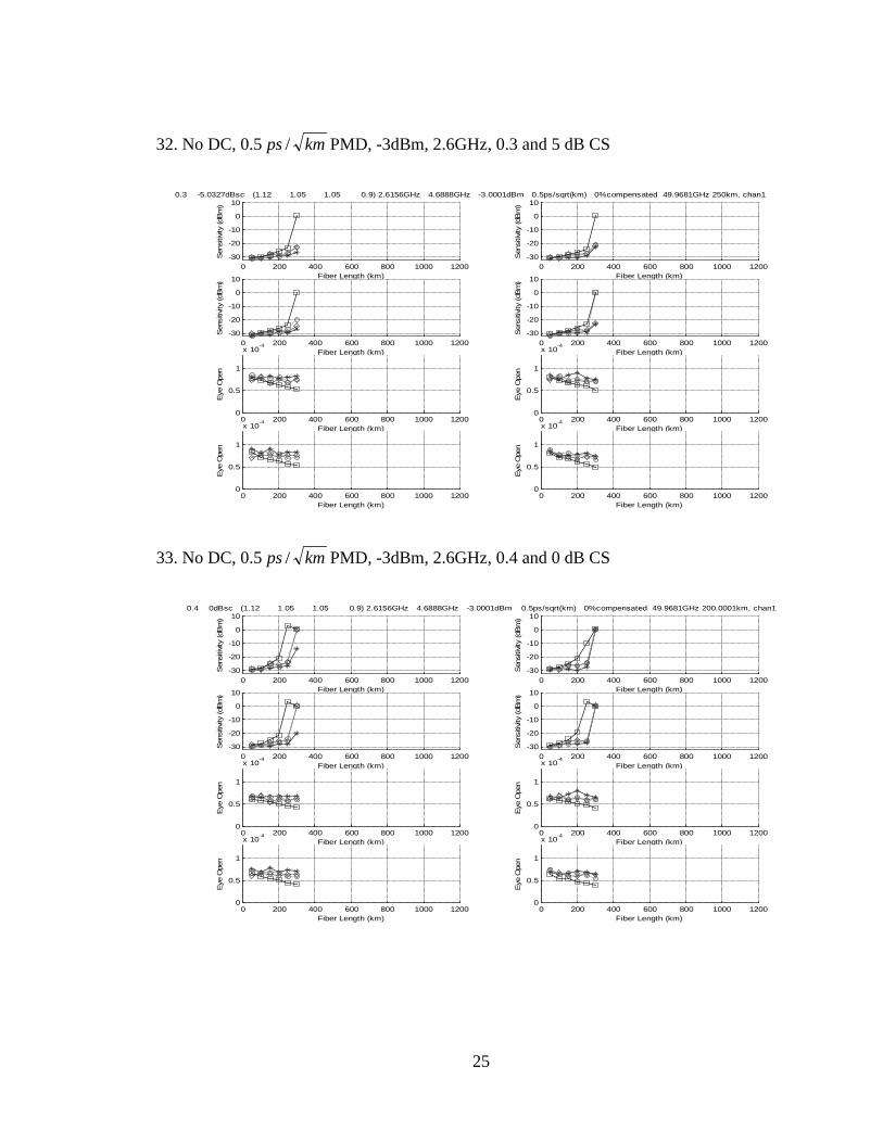
25

32. No DC, 0.5 kmps / PMD, -3dBm, 2.6GHz, 0.3 and 5 dB CS

0 200 400 600 800 1000 1200-30

-20

-10

0

10

Fiber Length (km)

Sen

sitiv

ity (dB

m)

0.3 -5.0327dBsc (1.12 1.05 1.05 0.9) 2.6156GHz 4.6888GHz -3.0001dBm

0 200 400 600 800 1000 1200-30

-20

-10

0

10

Fiber Length (km)

Sen

sitiv

ity (dB

m)

0.5ps/sqrt(km) 0%compensated 49.9681GHz 250km, chan1

0 200 400 600 800 1000 1200-30

-20

-10

0

10

Fiber Length (km)

Sen

sitiv

ity (dB

m)

0 200 400 600 800 1000 1200-30

-20

-10

0

10

Fiber Length (km)

Sen

sitiv

ity (dB

m)

0 200 400 600 800 1000 12000

0.5

1

x 10-4

Fiber Length (km)

Eye

Ope

n

0 200 400 600 800 1000 12000

0.5

1

x 10-4

Fiber Length (km)

Eye

Ope

n

0 200 400 600 800 1000 12000

0.5

1

x 10-4

Fiber Length (km)

Eye

Ope

n

0 200 400 600 800 1000 12000

0.5

1

x 10-4

Fiber Length (km)

Eye

Ope

n

33. No DC, 0.5 kmps / PMD, -3dBm, 2.6GHz, 0.4 and 0 dB CS

0 200 400 600 800 1000 1200-30

-20

-10

0

10

Fiber Length (km)

Sen

sitiv

ity (dB

m)

0.4 0dBsc (1.12 1.05 1.05 0.9) 2.6156GHz 4.6888GHz -3.0001dBm

0 200 400 600 800 1000 1200-30

-20

-10

0

10

Fiber Length (km)

Sen

sitiv

ity (dB

m)

0.5ps/sqrt(km) 0%compensated 49.9681GHz 200.0001km, chan1

0 200 400 600 800 1000 1200-30

-20

-10

0

10

Fiber Length (km)

Sen

sitiv

ity (dB

m)

0 200 400 600 800 1000 1200-30

-20

-10

0

10

Fiber Length (km)

Sen

sitiv

ity (dB

m)

0 200 400 600 800 1000 12000

0.5

1

x 10-4

Fiber Length (km)

Eye

Ope

n

0 200 400 600 800 1000 12000

0.5

1

x 10-4

Fiber Length (km)

Eye

Ope

n

0 200 400 600 800 1000 12000

0.5

1

x 10-4

Fiber Length (km)

Eye

Ope

n

0 200 400 600 800 1000 12000

0.5

1

x 10-4

Fiber Length (km)

Eye

Ope

n

1

Appendix 3: QPSK SCM results

1.DC, 0.1 kmps / PMD, 5dBm, 0.3 and 5 dB CS

0 200 400 600 800 1000 1200

-30

-20

-10

0

10

Fiber Length (km)

Sen

sitiv

ity (dB

m)

0.3 -5.0327dBsc (1 1) 4.0106GHz 7.2075GHz 5dBm

0 200 400 600 800 1000 1200

-30

-20

-10

0

10

Fiber Length (km)

Sen

sitiv

ity (dB

m)

0.1ps/sqrt(km) 100%compensated 49.9681GHz 1099.9996km, chan1

0 200 400 600 800 1000 1200

-30

-20

-10

0

10

Fiber Length (km)

Sen

sitiv

ity (dB

m)

0 200 400 600 800 1000 1200

-30

-20

-10

0

10

Fiber Length (km)

Sen

sitiv

ity (dB

m)

0 200 400 600 800 1000 12000

0.5

1

x 10-4

Fiber Length (km)

Eye

Ope

n

0 200 400 600 800 1000 12000

0.5

1

x 10-4

Fiber Length (km)E

ye O

pen

0 200 400 600 800 1000 12000

0.5

1

x 10-4

Fiber Length (km)

Eye

Ope

n

0 200 400 600 800 1000 12000

0.5

1

x 10-4

Fiber Length (km)

Eye

Ope

n

2

2. DC, 0.1 kmps / PMD, 5dBm, 0.4 and 0 dB CS

0 200 400 600 800 1000 1200

-30

-20

-10

0

10

Fiber Length (km)

Sen

sitiv

ity (dB

m)

0.4 0dBsc (1 1) 4.0106GHz 7.2075GHz 5dBm

0 200 400 600 800 1000 1200

-30

-20

-10

0

10

Fiber Length (km)

Sen

sitiv

ity (dB

m)

0.1ps/sqrt(km) 100%compensated 49.9681GHz 950.0004km, chan2

0 200 400 600 800 1000 1200

-30

-20

-10

0

10

Fiber Length (km)

Sen

sitiv

ity (dB

m)

0 200 400 600 800 1000 1200

-30

-20

-10

0

10

Fiber Length (km)

Sen

sitiv

ity (dB

m)

0 200 400 600 800 1000 12000

0.5

1

x 10-4

Fiber Length (km)

Eye

Ope

n

0 200 400 600 800 1000 12000

0.5

1

x 10-4

Fiber Length (km)

Eye

Ope

n0 200 400 600 800 1000 1200

0

0.5

1

x 10-4

Fiber Length (km)

Eye

Ope

n

0 200 400 600 800 1000 12000

0.5

1

x 10-4

Fiber Length (km)

Eye

Ope

n

3. DC, 0.1 kmps / PMD, 3dBm, 0.3 and 5 dB CS

0 200 400 600 800 1000 1200

-30

-20

-10

0

10

Fiber Length (km)

Sen

sitiv

ity (dB

m)

0.3 -5.0327dBsc (1 1) 4.0106GHz 7.2075GHz 3dBm

0 200 400 600 800 1000 1200

-30

-20

-10

0

10

Fiber Length (km)

Sen

sitiv

ity (dB

m)

0.1ps/sqrt(km) 100%compensated 49.9681GHz 1200km, chan1

0 200 400 600 800 1000 1200

-30

-20

-10

0

10

Fiber Length (km)

Sen

sitiv

ity (dB

m)

0 200 400 600 800 1000 1200

-30

-20

-10

0

10

Fiber Length (km)

Sen

sitiv

ity (dB

m)

0 200 400 600 800 1000 12000

0.5

1

1.5x 10

-4

Fiber Length (km)

Eye

Ope

n

0 200 400 600 800 1000 12000

0.5

1

1.5x 10

-4

Fiber Length (km)

Eye

Ope

n

0 200 400 600 800 1000 12000

0.5

1

1.5x 10

-4

Fiber Length (km)

Eye

Ope

n

0 200 400 600 800 1000 12000

0.5

1

1.5x 10

-4

Fiber Length (km)

Eye

Ope

n

3

4. DC, 0.1 kmps / PMD, 3dBm, 0.4 and 0 dB CS

0 200 400 600 800 1000 1200

-30

-20

-10

0

10

Fiber Length (km)

Sen

sitiv

ity (dB

m)

0.4 0dBsc (1 1) 4.0106GHz 7.2075GHz 3dBm

0 200 400 600 800 1000 1200

-30

-20

-10

0

10

Fiber Length (km)

Sen

sitiv

ity (dB

m)

0.1ps/sqrt(km) 100%compensated 49.9681GHz 900km, chan1

0 200 400 600 800 1000 1200

-30

-20

-10

0

10

Fiber Length (km)

Sen

sitiv

ity (dB

m)

0 200 400 600 800 1000 1200

-30

-20

-10

0

10

Fiber Length (km)

Sen

sitiv

ity (dB

m)

0 200 400 600 800 1000 12000

0.5

1

1.5x 10

-4

Fiber Length (km)

Eye

Ope

n

0 200 400 600 800 1000 12000

0.5

1

1.5x 10

-4

Fiber Length (km)

Eye

Ope

n0 200 400 600 800 1000 1200

0

0.5

1

1.5x 10

-4

Fiber Length (km)

Eye

Ope

n

0 200 400 600 800 1000 12000

0.5

1

1.5x 10

-4

Fiber Length (km)

Eye

Ope

n

5. DC, 0.1 kmps / PMD, 0dBm, 0.3 and 7 dB CS

0 200 400 600 800 1000 1200

-30

-20

-10

0

10

Fiber Length (km)

Sen

sitiv

ity (dB

m)

0.3 -7.0204dBsc (1 1) 4.0106GHz 7.2075GHz 0dBm

0 200 400 600 800 1000 1200

-30

-20

-10

0

10

Fiber Length (km)

Sen

sitiv

ity (dB

m)

0.1ps/sqrt(km) 100%compensated 49.9681GHz 750km, chan1

0 200 400 600 800 1000 1200

-30

-20

-10

0

10

Fiber Length (km)

Sen

sitiv

ity (dB

m)

0 200 400 600 800 1000 1200

-30

-20

-10

0

10

Fiber Length (km)

Sen

sitiv

ity (dB

m)

0 200 400 600 800 1000 12000

0.5

1

1.5

x 10-4

Fiber Length (km)

Eye

Ope

n

0 200 400 600 800 1000 12000

0.5

1

1.5

x 10-4

Fiber Length (km)

Eye

Ope

n

0 200 400 600 800 1000 12000

0.5

1

1.5

x 10-4

Fiber Length (km)

Eye

Ope

n

0 200 400 600 800 1000 12000

0.5

1

1.5

x 10-4

Fiber Length (km)

Eye

Ope

n

4

6. DC, 0.1 kmps / PMD, 0dBm, 0.4 and 0 dB CS

0 200 400 600 800 1000 1200

-30

-20

-10

0

10

Fiber Length (km)

Sen

sitiv

ity (dB

m)

0.4 0dBsc (1 1) 4.0106GHz 7.2075GHz 0dBm

0 200 400 600 800 1000 1200

-30

-20

-10

0

10

Fiber Length (km)

Sen

sitiv

ity (dB

m)

0.1ps/sqrt(km) 100%compensated 49.9681GHz 549.9998km, chan1

0 200 400 600 800 1000 1200

-30

-20

-10

0

10

Fiber Length (km)

Sen

sitiv

ity (dB

m)

0 200 400 600 800 1000 1200

-30

-20

-10

0

10

Fiber Length (km)

Sen

sitiv

ity (dB

m)

0 200 400 600 800 1000 12000

0.5

1

1.5

x 10-4

Fiber Length (km)

Eye

Ope

n

0 200 400 600 800 1000 12000

0.5

1

1.5

x 10-4

Fiber Length (km)

Eye

Ope

n0 200 400 600 800 1000 1200

0

0.5

1

1.5

x 10-4

Fiber Length (km)

Eye

Ope

n

0 200 400 600 800 1000 12000

0.5

1

1.5

x 10-4

Fiber Length (km)

Eye

Ope

n

7. DC, 0.1 kmps / PMD, -3dBm, 0.3 and 7 dB CS

0 200 400 600 800 1000 1200

-30

-20

-10

0

10

Fiber Length (km)

Sen

sitiv

ity (dB

m)

0.3 -7.0204dBsc (1 1) 4.0106GHz 7.2075GHz -3.0001dBm

0 200 400 600 800 1000 1200

-30

-20

-10

0

10

Fiber Length (km)

Sen

sitiv

ity (dB

m)

0.1ps/sqrt(km) 100%compensated 49.9681GHz 500.0002km, chan1

0 200 400 600 800 1000 1200

-30

-20

-10

0

10

Fiber Length (km)

Sen

sitiv

ity (dB

m)

0 200 400 600 800 1000 1200

-30

-20

-10

0

10

Fiber Length (km)

Sen

sitiv

ity (dB

m)

0 200 400 600 800 1000 12000

0.5

1

1.5

x 10-4

Fiber Length (km)

Eye

Ope

n

0 200 400 600 800 1000 12000

0.5

1

1.5

x 10-4

Fiber Length (km)

Eye

Ope

n

0 200 400 600 800 1000 12000

0.5

1

1.5

x 10-4

Fiber Length (km)

Eye

Ope

n

0 200 400 600 800 1000 12000

0.5

1

1.5

x 10-4

Fiber Length (km)

Eye

Ope

n

5

8. DC, 0.1 kmps / PMD, -3dBm, 0.4 and 0 dB CS

0 200 400 600 800 1000 1200

-30

-20

-10

0

10

Fiber Length (km)

Sen

sitiv

ity (dB

m)

0.4 0dBsc (1 1) 4.0106GHz 7.2075GHz -3.0001dBm

0 200 400 600 800 1000 1200

-30

-20

-10

0

10

Fiber Length (km)

Sen

sitiv

ity (dB

m)

0.1ps/sqrt(km) 100%compensated 49.9681GHz 350km, chan1

0 200 400 600 800 1000 1200

-30

-20

-10

0

10

Fiber Length (km)

Sen

sitiv

ity (dB

m)

0 200 400 600 800 1000 1200

-30

-20

-10

0

10

Fiber Length (km)

Sen

sitiv

ity (dB

m)

0 200 400 600 800 1000 12000

0.5

1

1.5

x 10-4

Fiber Length (km)

Eye

Ope

n

0 200 400 600 800 1000 12000

0.5

1

1.5

x 10-4

Fiber Length (km)

Eye

Ope

n0 200 400 600 800 1000 1200

0

0.5

1

1.5

x 10-4

Fiber Length (km)

Eye

Ope

n

0 200 400 600 800 1000 12000

0.5

1

1.5

x 10-4

Fiber Length (km)

Eye

Ope

n

9. No DC, 0.1 kmps / PMD, 5dBm, 0.3 and 5 dB CS

0 200 400 600 800 1000 1200

-30

-20

-10

0

10

Fiber Length (km)

Sen

sitiv

ity (dB

m)

0.3 -5.0327dBsc (1 1) 4.0106GHz 7.2075GHz 5dBm

0 200 400 600 800 1000 1200

-30

-20

-10

0

10

Fiber Length (km)

Sen

sitiv

ity (dB

m)

0.1ps/sqrt(km) 0%compensated 49.9681GHz 400km, chan2

0 200 400 600 800 1000 1200

-30

-20

-10

0

10

Fiber Length (km)

Sen

sitiv

ity (dB

m)

0 200 400 600 800 1000 1200

-30

-20

-10

0

10

Fiber Length (km)

Sen

sitiv

ity (dB

m)

0 200 400 600 800 1000 12000

0.5

1

1.5x 10

-4

Fiber Length (km)

Eye

Ope

n

0 200 400 600 800 1000 12000

0.5

1

1.5x 10

-4

Fiber Length (km)

Eye

Ope

n

0 200 400 600 800 1000 12000

0.5

1

1.5x 10

-4

Fiber Length (km)

Eye

Ope

n

0 200 400 600 800 1000 12000

0.5

1

1.5x 10

-4

Fiber Length (km)

Eye

Ope

n

6

10. No DC, 0.1 kmps / PMD, 5dBm, 0.4 and 0 dB CS

0 200 400 600 800 1000 1200

-30

-20

-10

0

10

Fiber Length (km)

Sen

sitiv

ity (dB

m)

0.4 0dBsc (1 1) 4.0106GHz 7.2075GHz 5dBm

0 200 400 600 800 1000 1200

-30

-20

-10

0

10

Fiber Length (km)

Sen

sitiv

ity (dB

m)

0.1ps/sqrt(km) 0%compensated 49.9681GHz 400km, chan2

0 200 400 600 800 1000 1200

-30

-20

-10

0

10

Fiber Length (km)

Sen

sitiv

ity (dB

m)

0 200 400 600 800 1000 1200

-30

-20

-10

0

10

Fiber Length (km)

Sen

sitiv

ity (dB

m)

0 200 400 600 800 1000 12000

0.5

1

1.5x 10

-4

Fiber Length (km)

Eye

Ope

n

0 200 400 600 800 1000 12000

0.5

1

1.5x 10

-4

Fiber Length (km)

Eye

Ope

n0 200 400 600 800 1000 1200

0

0.5

1

1.5x 10

-4

Fiber Length (km)

Eye

Ope

n

0 200 400 600 800 1000 12000

0.5

1

1.5x 10

-4

Fiber Length (km)

Eye

Ope

n

11. No DC, 0.1 kmps / PMD, 3dBm, 0.3 and 5 dB CS

0 200 400 600 800 1000 1200

-30

-20

-10

0

10

Fiber Length (km)

Sen

sitiv

ity (dB

m)

0.3 -5.0327dBsc (1 1) 4.0106GHz 7.2075GHz 3dBm

0 200 400 600 800 1000 1200

-30

-20

-10

0

10

Fiber Length (km)

Sen

sitiv

ity (dB

m)

0.1ps/sqrt(km) 0%compensated 49.9681GHz 450km, chan2

0 200 400 600 800 1000 1200

-30

-20

-10

0

10

Fiber Length (km)

Sen

sitiv

ity (dB

m)

0 200 400 600 800 1000 1200

-30

-20

-10

0

10

Fiber Length (km)

Sen

sitiv

ity (dB

m)

0 200 400 600 800 1000 12000

0.5

1

1.5x 10

-4

Fiber Length (km)

Eye

Ope

n

0 200 400 600 800 1000 12000

0.5

1

1.5x 10

-4

Fiber Length (km)

Eye

Ope

n

0 200 400 600 800 1000 12000

0.5

1

1.5x 10

-4

Fiber Length (km)

Eye

Ope

n

0 200 400 600 800 1000 12000

0.5

1

1.5x 10

-4

Fiber Length (km)

Eye

Ope

n

7

12. No DC, 0.1 kmps / PMD, 3dBm, 0.4 and 0 dB CS

0 200 400 600 800 1000 1200

-30

-20

-10

0

10

Fiber Length (km)

Sen

sitiv

ity (dB

m)

0.4 0dBsc (1 1) 4.0106GHz 7.2075GHz 3dBm

0 200 400 600 800 1000 1200

-30

-20

-10

0

10

Fiber Length (km)

Sen

sitiv

ity (dB

m)

0.1ps/sqrt(km) 0%compensated 49.9681GHz 450km, chan2

0 200 400 600 800 1000 1200

-30

-20

-10

0

10

Fiber Length (km)

Sen

sitiv

ity (dB

m)

0 200 400 600 800 1000 1200

-30

-20

-10

0

10

Fiber Length (km)

Sen

sitiv

ity (dB

m)

0 200 400 600 800 1000 12000

0.5

1

1.5x 10

-4

Fiber Length (km)

Eye

Ope

n

0 200 400 600 800 1000 12000

0.5

1

1.5x 10

-4

Fiber Length (km)

Eye

Ope

n0 200 400 600 800 1000 1200

0

0.5

1

1.5x 10

-4

Fiber Length (km)

Eye

Ope

n

0 200 400 600 800 1000 12000

0.5

1

1.5x 10

-4

Fiber Length (km)

Eye

Ope

n

13. No DC, 0.1 kmps / PMD, 0dBm, 0.3 and 7 dB CS

0 200 400 600 800 1000 1200

-30

-20

-10

0

10

Fiber Length (km)

Sen

sitiv

ity (dB

m)

0.3 -7.0204dBsc (1 1) 4.0106GHz 7.2075GHz 0dBm

0 200 400 600 800 1000 1200

-30

-20

-10

0

10

Fiber Length (km)

Sen

sitiv

ity (dB

m)

0.1ps/sqrt(km) 0%compensated 49.9681GHz 250km, chan1

0 200 400 600 800 1000 1200

-30

-20

-10

0

10

Fiber Length (km)

Sen

sitiv

ity (dB

m)

0 200 400 600 800 1000 1200

-30

-20

-10

0

10

Fiber Length (km)

Sen

sitiv

ity (dB

m)

0 200 400 600 800 1000 12000

0.5

1

1.5

x 10-4

Fiber Length (km)

Eye

Ope

n

0 200 400 600 800 1000 12000

0.5

1

1.5

x 10-4

Fiber Length (km)

Eye

Ope

n

0 200 400 600 800 1000 12000

0.5

1

1.5

x 10-4

Fiber Length (km)

Eye

Ope

n

0 200 400 600 800 1000 12000

0.5

1

1.5

x 10-4

Fiber Length (km)

Eye

Ope

n

8

14. No DC, 0.1 kmps / PMD, 0dBm, 0.4 and 0 dB CS

0 200 400 600 800 1000 1200

-30

-20

-10

0

10

Fiber Length (km)

Sen

sitiv

ity (dB

m)

0.4 0dBsc (1 1) 4.0106GHz 7.2075GHz 0dBm

0 200 400 600 800 1000 1200

-30

-20

-10

0

10

Fiber Length (km)

Sen

sitiv

ity (dB

m)

0.1ps/sqrt(km) 0%compensated 49.9681GHz 250km, chan3

0 200 400 600 800 1000 1200

-30

-20

-10

0

10

Fiber Length (km)

Sen

sitiv

ity (dB

m)

0 200 400 600 800 1000 1200

-30

-20

-10

0

10

Fiber Length (km)

Sen

sitiv

ity (dB

m)

0 200 400 600 800 1000 12000

0.5

1

1.5

x 10-4

Fiber Length (km)

Eye

Ope

n

0 200 400 600 800 1000 12000

0.5

1

1.5

x 10-4

Fiber Length (km)

Eye

Ope

n0 200 400 600 800 1000 1200

0

0.5

1

1.5

x 10-4

Fiber Length (km)

Eye

Ope

n

0 200 400 600 800 1000 12000

0.5

1

1.5

x 10-4

Fiber Length (km)

Eye

Ope

n

15. No DC, 0.1 kmps / PMD, -3dBm, 0.3 and 7 dB CS

0 200 400 600 800 1000 1200

-30

-20

-10

0

10

Fiber Length (km)

Sen

sitiv

ity (dB

m)

0.3 -7.0204dBsc (1 1) 4.0106GHz 7.2075GHz -3.0001dBm

0 200 400 600 800 1000 1200

-30

-20

-10

0

10

Fiber Length (km)

Sen

sitiv

ity (dB

m)

0.1ps/sqrt(km) 0%compensated 49.9681GHz 250km, chan1

0 200 400 600 800 1000 1200

-30

-20

-10

0

10

Fiber Length (km)

Sen

sitiv

ity (dB

m)

0 200 400 600 800 1000 1200

-30

-20

-10

0

10

Fiber Length (km)

Sen

sitiv

ity (dB

m)

0 200 400 600 800 1000 12000

0.5

1

1.5

x 10-4

Fiber Length (km)

Eye

Ope

n

0 200 400 600 800 1000 12000

0.5

1

1.5

x 10-4

Fiber Length (km)

Eye

Ope

n

0 200 400 600 800 1000 12000

0.5

1

1.5

x 10-4

Fiber Length (km)

Eye

Ope

n

0 200 400 600 800 1000 12000

0.5

1

1.5

x 10-4

Fiber Length (km)

Eye

Ope

n

9

16. No DC, 0.1 kmps / PMD, -3dBm, 0.4 and 0 dB CS

0 200 400 600 800 1000 1200

-30

-20

-10

0

10

Fiber Length (km)

Sen

sitiv

ity (dB

m)

0.4 0dBsc (1 1) 4.0106GHz 7.2075GHz -3.0001dBm

0 200 400 600 800 1000 1200

-30

-20

-10

0

10

Fiber Length (km)

Sen

sitiv

ity (dB

m)

0.1ps/sqrt(km) 0%compensated 49.9681GHz 250km, chan1

0 200 400 600 800 1000 1200

-30

-20

-10

0

10

Fiber Length (km)

Sen

sitiv

ity (dB

m)

0 200 400 600 800 1000 1200

-30

-20

-10

0

10

Fiber Length (km)

Sen

sitiv

ity (dB

m)

0 200 400 600 800 1000 12000

0.5

1

1.5

x 10-4

Fiber Length (km)

Eye

Ope

n

0 200 400 600 800 1000 12000

0.5

1

1.5

x 10-4

Fiber Length (km)

Eye

Ope

n0 200 400 600 800 1000 1200

0

0.5

1

1.5

x 10-4

Fiber Length (km)

Eye

Ope

n

0 200 400 600 800 1000 12000

0.5

1

1.5

x 10-4

Fiber Length (km)

Eye

Ope

n

17. DC, 0.5 kmps / PMD, 5dBm, 0.3 and 5 dB CS

0 200 400 600 800 1000 1200

-30

-20

-10

0

10

Fiber Length (km)

Sen

sitiv

ity (dB

m)

0.3 -5.0327dBsc (1 1) 4.0106GHz 7.2075GHz 5dBm

0 200 400 600 800 1000 1200

-30

-20

-10

0

10

Fiber Length (km)

Sen

sitiv

ity (dB

m)

0.5ps/sqrt(km) 100%compensated 49.9681GHz 750km, chan1

0 200 400 600 800 1000 1200

-30

-20

-10

0

10

Fiber Length (km)

Sen

sitiv

ity (dB

m)

0 200 400 600 800 1000 1200

-30

-20

-10

0

10

Fiber Length (km)

Sen

sitiv

ity (dB

m)

0 200 400 600 800 1000 12000

0.5

1

1.5x 10

-4

Fiber Length (km)

Eye

Ope

n

0 200 400 600 800 1000 12000

0.5

1

1.5x 10

-4

Fiber Length (km)

Eye

Ope

n

0 200 400 600 800 1000 12000

0.5

1

1.5x 10

-4

Fiber Length (km)

Eye

Ope

n

0 200 400 600 800 1000 12000

0.5

1

1.5x 10

-4

Fiber Length (km)

Eye

Ope

n

10

18. DC, 0.5 kmps / PMD, 5dBm, 0.4 and 0 dB CS

0 200 400 600 800 1000 1200

-30

-20

-10

0

10

Fiber Length (km)

Sen

sitiv

ity (dB

m)

0.4 0dBsc (1 1) 4.0106GHz 7.2075GHz 5dBm

0 200 400 600 800 1000 1200

-30

-20

-10

0

10

Fiber Length (km)

Sen

sitiv

ity (dB

m)

0.5ps/sqrt(km) 100%compensated 49.9681GHz 649.9998km, chan1

0 200 400 600 800 1000 1200

-30

-20

-10

0

10

Fiber Length (km)

Sen

sitiv

ity (dB

m)

0 200 400 600 800 1000 1200

-30

-20

-10

0

10

Fiber Length (km)

Sen

sitiv

ity (dB

m)

0 200 400 600 800 1000 12000

0.5

1

1.5x 10

-4

Fiber Length (km)

Eye

Ope

n

0 200 400 600 800 1000 12000

0.5

1

1.5x 10

-4

Fiber Length (km)

Eye

Ope

n0 200 400 600 800 1000 1200

0

0.5

1

1.5x 10

-4

Fiber Length (km)

Eye

Ope

n

0 200 400 600 800 1000 12000

0.5

1

1.5x 10

-4

Fiber Length (km)

Eye

Ope

n

19. DC, 0.5 kmps / PMD, 3dBm, 0.3 and 5 dB CS

0 200 400 600 800 1000 1200

-30

-20

-10

0

10

Fiber Length (km)

Sen

sitiv

ity (dB

m)

0.3 -5.0327dBsc (1 1) 4.0106GHz 7.2075GHz 3dBm

0 200 400 600 800 1000 1200

-30

-20

-10

0

10

Fiber Length (km)

Sen

sitiv

ity (dB

m)

0.5ps/sqrt(km) 100%compensated 49.9681GHz 700.0002km, chan1

0 200 400 600 800 1000 1200

-30

-20

-10

0

10

Fiber Length (km)

Sen

sitiv

ity (dB

m)

0 200 400 600 800 1000 1200

-30

-20

-10

0

10

Fiber Length (km)

Sen

sitiv

ity (dB

m)

0 200 400 600 800 1000 12000

0.5

1

1.5x 10

-4

Fiber Length (km)

Eye

Ope

n

0 200 400 600 800 1000 12000

0.5

1

1.5x 10

-4

Fiber Length (km)

Eye

Ope

n

0 200 400 600 800 1000 12000

0.5

1

1.5x 10

-4

Fiber Length (km)

Eye

Ope

n

0 200 400 600 800 1000 12000

0.5

1

1.5x 10

-4

Fiber Length (km)

Eye

Ope

n

11

20. DC, 0.5 kmps / PMD, 3dBm, 0.4 and 0 dB CS

0 200 400 600 800 1000 1200

-30

-20

-10

0

10

Fiber Length (km)

Sen

sitiv

ity (dB

m)

0.4 0dBsc (1 1) 4.0106GHz 7.2075GHz 3dBm

0 200 400 600 800 1000 1200

-30

-20

-10

0

10

Fiber Length (km)

Sen

sitiv

ity (dB

m)

0.5ps/sqrt(km) 100%compensated 49.9681GHz 500.0002km, chan2

0 200 400 600 800 1000 1200

-30

-20

-10

0

10

Fiber Length (km)

Sen

sitiv

ity (dB

m)

0 200 400 600 800 1000 1200

-30

-20

-10

0

10

Fiber Length (km)

Sen

sitiv

ity (dB

m)

0 200 400 600 800 1000 12000

0.5

1

1.5x 10

-4

Fiber Length (km)

Eye

Ope

n

0 200 400 600 800 1000 12000

0.5

1

1.5x 10

-4

Fiber Length (km)

Eye

Ope

n0 200 400 600 800 1000 1200

0

0.5

1

1.5x 10

-4

Fiber Length (km)

Eye

Ope

n

0 200 400 600 800 1000 12000

0.5

1

1.5x 10

-4

Fiber Length (km)

Eye

Ope

n

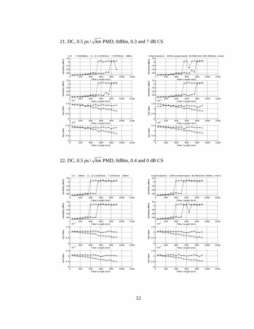
12

21. DC, 0.5 kmps / PMD, 0dBm, 0.3 and 7 dB CS

0 200 400 600 800 1000 1200

-30

-20

-10

0

10

Fiber Length (km)

Sen

sitiv

ity (dB

m)

0.3 -7.0204dBsc (1 1) 4.0106GHz 7.2075GHz 0dBm

0 200 400 600 800 1000 1200

-30

-20

-10

0

10

Fiber Length (km)

Sen

sitiv

ity (dB

m)

0.5ps/sqrt(km) 100%compensated 49.9681GHz 500.0002km, chan1

0 200 400 600 800 1000 1200

-30

-20

-10

0

10

Fiber Length (km)

Sen

sitiv

ity (dB

m)

0 200 400 600 800 1000 1200

-30

-20

-10

0

10

Fiber Length (km)

Sen

sitiv

ity (dB

m)

0 200 400 600 800 1000 12000

0.5

1

1.5

x 10-4

Fiber Length (km)

Eye

Ope

n

0 200 400 600 800 1000 12000

0.5

1

1.5

x 10-4

Fiber Length (km)

Eye

Ope

n

0 200 400 600 800 1000 12000

0.5

1

1.5

x 10-4

Fiber Length (km)

Eye

Ope

n

0 200 400 600 800 1000 12000

0.5

1

1.5

x 10-4

Fiber Length (km)

Eye

Ope

n

22. DC, 0.5 kmps / PMD, 0dBm, 0.4 and 0 dB CS

0 200 400 600 800 1000 1200

-30

-20

-10

0

10

Fiber Length (km)

Sen

sitiv

ity (dB

m)

0.4 0dBsc (1 1) 4.0106GHz 7.2075GHz 0dBm

0 200 400 600 800 1000 1200

-30

-20

-10

0

10

Fiber Length (km)

Sen

sitiv

ity (dB

m)

0.5ps/sqrt(km) 100%compensated 49.9681GHz 350km, chan1

0 200 400 600 800 1000 1200

-30

-20

-10

0

10

Fiber Length (km)

Sen

sitiv

ity (dB

m)

0 200 400 600 800 1000 1200

-30

-20

-10

0

10

Fiber Length (km)

Sen

sitiv

ity (dB

m)

0 200 400 600 800 1000 12000

0.5

1

1.5

x 10-4

Fiber Length (km)

Eye

Ope

n

0 200 400 600 800 1000 12000

0.5

1

1.5

x 10-4

Fiber Length (km)

Eye

Ope

n

0 200 400 600 800 1000 12000

0.5

1

1.5

x 10-4

Fiber Length (km)

Eye

Ope

n

0 200 400 600 800 1000 12000

0.5

1

1.5

x 10-4

Fiber Length (km)

Eye

Ope

n

13

23. DC, 0.5 kmps / PMD, -3dBm, 0.3 and 7 dB CS

0 200 400 600 800 1000 1200

-30

-20

-10

0

10

Fiber Length (km)

Sen

sitiv

ity (dB

m)

0.3 -7.0204dBsc (1 1) 4.0106GHz 7.2075GHz -3.0001dBm

0 200 400 600 800 1000 1200

-30

-20

-10

0

10

Fiber Length (km)

Sen

sitiv

ity (dB

m)

0.5ps/sqrt(km) 100%compensated 49.9681GHz 350km, chan1

0 200 400 600 800 1000 1200

-30

-20

-10

0

10

Fiber Length (km)

Sen

sitiv

ity (dB

m)

0 200 400 600 800 1000 1200

-30

-20

-10

0

10

Fiber Length (km)

Sen

sitiv

ity (dB

m)

0 200 400 600 800 1000 12000

0.5

1

1.5

x 10-4

Fiber Length (km)

Eye

Ope

n

0 200 400 600 800 1000 12000

0.5

1

1.5

x 10-4

Fiber Length (km)

Eye

Ope

n

0 200 400 600 800 1000 12000

0.5

1

1.5

x 10-4

Fiber Length (km)

Eye

Ope

n

0 200 400 600 800 1000 12000

0.5

1

1.5

x 10-4

Fiber Length (km)

Eye

Ope

n

24. DC, 0.5 kmps / PMD, 0dBm, 0.4 and 0 dB CS

0 200 400 600 800 1000 1200

-30

-20

-10

0

10

Fiber Length (km)

Sen

sitiv

ity (dB

m)

0.4 0dBsc (1 1) 4.0106GHz 7.2075GHz -3.0001dBm

0 200 400 600 800 1000 1200

-30

-20

-10

0

10

Fiber Length (km)

Sen

sitiv

ity (dB

m)

0.5ps/sqrt(km) 100%compensated 49.9681GHz 250km, chan1

0 200 400 600 800 1000 1200

-30

-20

-10

0

10

Fiber Length (km)

Sen

sitiv

ity (dB

m)

0 200 400 600 800 1000 1200

-30

-20

-10

0

10

Fiber Length (km)

Sen

sitiv

ity (dB

m)

0 200 400 600 800 1000 12000

0.5

1

1.5

x 10-4

Fiber Length (km)

Eye

Ope

n

0 200 400 600 800 1000 12000

0.5

1

1.5

x 10-4

Fiber Length (km)

Eye

Ope

n

0 200 400 600 800 1000 12000

0.5

1

1.5

x 10-4

Fiber Length (km)

Eye

Ope

n

0 200 400 600 800 1000 12000

0.5

1

1.5

x 10-4

Fiber Length (km)

Eye

Ope

n

14

25. No DC, 0.5 kmps / PMD, 5dBm, 0.3 and 5 dB CS

0 200 400 600 800 1000 1200

-30

-20

-10

0

10

Fiber Length (km)

Sen

sitiv

ity (dB

m)

0.3 -5.0327dBsc (1 1) 4.0106GHz 7.2075GHz 5dBm

0 200 400 600 800 1000 1200

-30

-20

-10

0

10

Fiber Length (km)

Sen

sitiv

ity (dB

m)

0.5ps/sqrt(km) 0%compensated 49.9681GHz 400km, chan2

0 200 400 600 800 1000 1200

-30

-20

-10

0

10

Fiber Length (km)

Sen

sitiv

ity (dB

m)

0 200 400 600 800 1000 1200

-30

-20

-10

0

10

Fiber Length (km)

Sen

sitiv

ity (dB

m)

0 200 400 600 800 1000 12000

0.5

1

1.5x 10

-4

Fiber Length (km)

Eye

Ope

n

0 200 400 600 800 1000 12000

0.5

1

1.5x 10

-4

Fiber Length (km)

Eye

Ope

n0 200 400 600 800 1000 1200

0

0.5

1

1.5x 10

-4

Fiber Length (km)

Eye

Ope

n

0 200 400 600 800 1000 12000

0.5

1

1.5x 10

-4

Fiber Length (km)

Eye

Ope

n

26. No DC, 0.5 kmps / PMD, 5dBm, 0.4 and 0 dB CS

0 200 400 600 800 1000 1200

-30

-20

-10

0

10

Fiber Length (km)

Sen

sitiv

ity (dB

m)

0.4 0dBsc (1 1) 4.0106GHz 7.2075GHz 5dBm

0 200 400 600 800 1000 1200

-30

-20

-10

0

10

Fiber Length (km)

Sen

sitiv

ity (dB

m)

0.5ps/sqrt(km) 0%compensated 49.9681GHz 400km, chan1

0 200 400 600 800 1000 1200

-30

-20

-10

0

10

Fiber Length (km)

Sen

sitiv

ity (dB

m)

0 200 400 600 800 1000 1200

-30

-20

-10

0

10

Fiber Length (km)

Sen

sitiv

ity (dB

m)

0 200 400 600 800 1000 12000

0.5

1

1.5x 10

-4

Fiber Length (km)

Eye

Ope

n

0 200 400 600 800 1000 12000

0.5

1

1.5x 10

-4

Fiber Length (km)

Eye

Ope

n

0 200 400 600 800 1000 12000

0.5

1

1.5x 10

-4

Fiber Length (km)

Eye

Ope

n

0 200 400 600 800 1000 12000

0.5

1

1.5x 10

-4

Fiber Length (km)

Eye

Ope

n

15

27. No DC, 0.5 kmps / PMD, 3dBm, 0.3 and 5 dB CS

0 200 400 600 800 1000 1200

-30

-20

-10

0

10

Fiber Length (km)

Sen

sitiv

ity (dB

m)

0.3 -5.0327dBsc (1 1) 4.0106GHz 7.2075GHz 3dBm

0 200 400 600 800 1000 1200

-30

-20

-10

0

10

Fiber Length (km)

Sen

sitiv

ity (dB

m)

0.5ps/sqrt(km) 0%compensated 49.9681GHz 450km, chan2

0 200 400 600 800 1000 1200

-30

-20

-10

0

10

Fiber Length (km)

Sen

sitiv

ity (dB

m)

0 200 400 600 800 1000 1200

-30

-20

-10

0

10

Fiber Length (km)

Sen

sitiv

ity (dB

m)

0 200 400 600 800 1000 12000

0.5

1

1.5x 10

-4

Fiber Length (km)

Eye

Ope

n

0 200 400 600 800 1000 12000

0.5

1

1.5x 10

-4

Fiber Length (km)

Eye

Ope

n0 200 400 600 800 1000 1200

0

0.5

1

1.5x 10

-4

Fiber Length (km)

Eye

Ope

n

0 200 400 600 800 1000 12000

0.5

1

1.5x 10

-4

Fiber Length (km)

Eye

Ope

n

28. No DC, 0.5 kmps / PMD, 3dBm, 0.4 and 0 dB CS

0 200 400 600 800 1000 1200

-30

-20

-10

0

10

Fiber Length (km)

Sen

sitiv

ity (dB

m)

0.4 0dBsc (1 1) 4.0106GHz 7.2075GHz 3dBm

0 200 400 600 800 1000 1200

-30

-20

-10

0

10

Fiber Length (km)

Sen

sitiv

ity (dB

m)

0.5ps/sqrt(km) 0%compensated 49.9681GHz 450km, chan2

0 200 400 600 800 1000 1200

-30

-20

-10

0

10

Fiber Length (km)

Sen

sitiv

ity (dB

m)

0 200 400 600 800 1000 1200

-30

-20

-10

0

10

Fiber Length (km)

Sen

sitiv

ity (dB

m)

0 200 400 600 800 1000 12000

0.5

1

x 10-4

Fiber Length (km)

Eye

Ope

n

0 200 400 600 800 1000 12000

0.5

1

x 10-4

Fiber Length (km)

Eye

Ope

n

0 200 400 600 800 1000 12000

0.5

1

x 10-4

Fiber Length (km)

Eye

Ope

n

0 200 400 600 800 1000 12000

0.5

1

x 10-4

Fiber Length (km)

Eye

Ope

n

16

29. No DC, 0.5 kmps / PMD, 0dBm, 0.3 and 7 dB CS

0 200 400 600 800 1000 1200

-30

-20

-10

0

10

Fiber Length (km)

Sen

sitiv

ity (dB

m)

0.3 -7.0204dBsc (1 1) 4.0106GHz 7.2075GHz 0dBm

0 200 400 600 800 1000 1200

-30

-20

-10

0

10

Fiber Length (km)

Sen

sitiv

ity (dB

m)

0.5ps/sqrt(km) 0%compensated 49.9681GHz 250km, chan1

0 200 400 600 800 1000 1200

-30

-20

-10

0

10

Fiber Length (km)

Sen

sitiv

ity (dB

m)

0 200 400 600 800 1000 1200

-30

-20

-10

0

10

Fiber Length (km)

Sen

sitiv

ity (dB

m)

0 200 400 600 800 1000 12000

0.5

1

1.5

x 10-4

Fiber Length (km)

Eye

Ope

n

0 200 400 600 800 1000 12000

0.5

1

1.5

x 10-4

Fiber Length (km)

Eye

Ope

n

0 200 400 600 800 1000 12000

0.5

1

1.5

x 10-4

Fiber Length (km)

Eye

Ope

n

0 200 400 600 800 1000 12000

0.5

1

1.5

x 10-4

Fiber Length (km)

Eye

Ope

n

30. No DC, 0.5 kmps / PMD, 0dBm, 0.4 and 0 dB CS

0 200 400 600 800 1000 1200

-30

-20

-10

0

10

Fiber Length (km)

Sen

sitiv

ity (dB

m)

0.4 0dBsc (1 1) 4.0106GHz 7.2075GHz 0dBm

0 200 400 600 800 1000 1200

-30

-20

-10

0

10

Fiber Length (km)

Sen

sitiv

ity (dB

m)

0.5ps/sqrt(km) 0%compensated 49.9681GHz 250km, chan3

0 200 400 600 800 1000 1200

-30

-20

-10

0

10

Fiber Length (km)

Sen

sitiv

ity (dB

m)

0 200 400 600 800 1000 1200

-30

-20

-10

0

10

Fiber Length (km)

Sen

sitiv

ity (dB

m)

0 200 400 600 800 1000 12000

0.5

1

1.5

x 10-4

Fiber Length (km)

Eye

Ope

n

0 200 400 600 800 1000 12000

0.5

1

1.5

x 10-4

Fiber Length (km)

Eye

Ope

n

0 200 400 600 800 1000 12000

0.5

1

1.5

x 10-4

Fiber Length (km)

Eye

Ope

n

0 200 400 600 800 1000 12000

0.5

1

1.5

x 10-4

Fiber Length (km)

Eye

Ope

n

17

31. No DC, 0.5 kmps / PMD, -3dBm, 0.3 and 7 dB CS

0 200 400 600 800 1000 1200

-30

-20

-10

0

10

Fiber Length (km)

Sen

sitiv

ity (dB

m)

0.3 -7.0204dBsc (1 1) 4.0106GHz 7.2075GHz -3.0001dBm

0 200 400 600 800 1000 1200

-30

-20

-10

0

10

Fiber Length (km)

Sen

sitiv

ity (dB

m)

0.5ps/sqrt(km) 0%compensated 49.9681GHz 250km, chan1

0 200 400 600 800 1000 1200

-30

-20

-10

0

10

Fiber Length (km)

Sen

sitiv

ity (dB

m)

0 200 400 600 800 1000 1200

-30

-20

-10

0

10

Fiber Length (km)

Sen

sitiv

ity (dB

m)

0 200 400 600 800 1000 12000

0.5

1

1.5

x 10-4

Fiber Length (km)

Eye

Ope

n

0 200 400 600 800 1000 12000

0.5

1

1.5

x 10-4

Fiber Length (km)

Eye

Ope

n

0 200 400 600 800 1000 12000

0.5

1

1.5

x 10-4

Fiber Length (km)

Eye

Ope

n

0 200 400 600 800 1000 12000

0.5

1

1.5

x 10-4

Fiber Length (km)

Eye

Ope

n

32. No DC, 0.5 kmps / PMD, -3dBm, 0.4 and 0 dB CS

0 200 400 600 800 1000 1200

-30

-20

-10

0

10

Fiber Length (km)

Sen

sitiv

ity (dB

m)

0.4 0dBsc (1 1) 4.0106GHz 7.2075GHz -3.0001dBm

0 200 400 600 800 1000 1200

-30

-20

-10

0

10

Fiber Length (km)

Sen

sitiv

ity (dB

m)

0.5ps/sqrt(km) 0%compensated 49.9681GHz 250km, chan1

0 200 400 600 800 1000 1200

-30

-20

-10

0

10

Fiber Length (km)

Sen

sitiv

ity (dB

m)

0 200 400 600 800 1000 1200

-30

-20

-10

0

10

Fiber Length (km)

Sen

sitiv

ity (dB

m)

0 200 400 600 800 1000 12000

0.5

1

1.5

x 10-4

Fiber Length (km)

Eye

Ope

n

0 200 400 600 800 1000 12000

0.5

1

1.5

x 10-4

Fiber Length (km)

Eye

Ope

n

0 200 400 600 800 1000 12000

0.5

1

1.5

x 10-4

Fiber Length (km)

Eye

Ope

n

0 200 400 600 800 1000 12000

0.5

1

1.5

x 10-4

Fiber Length (km)

Eye

Ope

n

1

Appendix 4: ASK SCM resultsDC, 0.1 kmps / PMD, 3dBm, 0.3 and -35 dB CS

0 200 400 600 800 1000 1200

-30

-20

-10

0

10

Fiber Length (km)

Sen

sitiv

ity (dB

m)

0.3 -35.1223dBsc (1 1 1 1) 2.8094GHz 4.7081GHz 3dBm

0 200 400 600 800 1000 1200

-30

-20

-10

0

10

Fiber Length (km)

Sen

sitiv

ity (dB

m)

0.1ps/sqrt(km) 100%compensated 49.9681GHz 50km, chan1

0 200 400 600 800 1000 1200

-30

-20

-10

0

10

Fiber Length (km)

Sen

sitiv

ity (dB

m)

0 200 400 600 800 1000 1200

-30

-20

-10

0

10

Fiber Length (km)

Sen

sitiv

ity (dB

m)

0 200 400 600 800 1000 12000

0.5

1

x 10-4

Fiber Length (km)

Eye

Ope

n

0 200 400 600 800 1000 12000

0.5

1

x 10-4

Fiber Length (km)

Eye

Ope

n0 200 400 600 800 1000 1200

0

0.5

1

x 10-4

Fiber Length (km)

Eye

Ope

n

0 200 400 600 800 1000 12000

0.5

1

x 10-4

Fiber Length (km)

Eye

Ope

n

DC, 0.1 kmps / PMD, 0dBm, 0.3 and -35 dB CS

0 200 400 600 800 1000 1200

-30

-20

-10

0

10

Fiber Length (km)

Sen

sitiv

ity (dB

m)

0.3 -35.1223dBsc (1 1 1 1) 2.8094GHz 4.7081GHz 0dBm

0 200 400 600 800 1000 1200

-30

-20

-10

0

10

Fiber Length (km)

Sen

sitiv

ity (dB

m)

0.1ps/sqrt(km) 100%compensated 49.9681GHz 200.0001km, chan1

0 200 400 600 800 1000 1200

-30

-20

-10

0

10

Fiber Length (km)

Sen

sitiv

ity (dB

m)

0 200 400 600 800 1000 1200

-30

-20

-10

0

10

Fiber Length (km)

Sen

sitiv

ity (dB

m)

0 200 400 600 800 1000 12000

0.5

1

x 10-4

Fiber Length (km)

Eye

Ope

n

0 200 400 600 800 1000 12000

0.5

1

x 10-4

Fiber Length (km)

Eye

Ope

n

0 200 400 600 800 1000 12000

0.5

1

x 10-4

Fiber Length (km)

Eye

Ope

n

0 200 400 600 800 1000 12000

0.5

1

x 10-4

Fiber Length (km)

Eye

Ope

n

2

DC, 0.1 kmps / PMD, -3dBm, 0.3 and -35 dB CS

0 200 400 600 800 1000 1200

-30

-20

-10

0

10

Fiber Length (km)

Sen

sitiv

ity (dB

m)

0.3 -35.1223dBsc (1 1 1 1) 2.8094GHz 4.7081GHz -3.0001dBm

0 200 400 600 800 1000 1200

-30

-20

-10

0

10

Fiber Length (km)

Sen

sitiv

ity (dB

m)

0.1ps/sqrt(km) 100%compensated 49.9681GHz 250km, chan1

0 200 400 600 800 1000 1200

-30

-20

-10

0

10

Fiber Length (km)

Sen

sitiv

ity (dB

m)

0 200 400 600 800 1000 1200

-30

-20

-10

0

10

Fiber Length (km)

Sen

sitiv

ity (dB

m)

0 200 400 600 800 1000 12000

0.5

1

x 10-4

Fiber Length (km)

Eye

Ope

n

0 200 400 600 800 1000 12000

0.5

1

x 10-4

Fiber Length (km)

Eye

Ope

n

0 200 400 600 800 1000 12000

0.5

1

x 10-4

Fiber Length (km)

Eye

Ope

n

0 200 400 600 800 1000 12000

0.5

1

x 10-4

Fiber Length (km)

Eye

Ope

n

DC, 0.1 kmps / PMD, -6dBm, 0.3 and -35 dB CS

0 200 400 600 800 1000 1200

-30

-20

-10

0

10

Fiber Length (km)

Sen

sitiv

ity (dB

m)

0.3 -35.1223dBsc (1 1 1 1) 2.8094GHz 4.7081GHz -5.9998dBm

0 200 400 600 800 1000 1200

-30

-20

-10

0

10

Fiber Length (km)

Sen

sitiv

ity (dB

m)

0.1ps/sqrt(km) 100%compensated 49.9681GHz 250km, chan1

0 200 400 600 800 1000 1200

-30

-20

-10

0

10

Fiber Length (km)

Sen

sitiv

ity (dB

m)

0 200 400 600 800 1000 1200

-30

-20

-10

0

10

Fiber Length (km)

Sen

sitiv

ity (dB

m)

0 200 400 600 800 1000 12000

0.5

1

x 10-4

Fiber Length (km)

Eye

Ope

n

0 200 400 600 800 1000 12000

0.5

1

x 10-4

Fiber Length (km)

Eye

Ope

n

0 200 400 600 800 1000 12000

0.5

1

x 10-4

Fiber Length (km)

Eye

Ope

n

0 200 400 600 800 1000 12000

0.5

1

x 10-4

Fiber Length (km)

Eye

Ope

n

3

No DC, 0.1 kmps / PMD, 3dBm, 0.3 and -35 dB CS

0 200 400 600 800 1000 1200

-30

-20

-10

0

10

Fiber Length (km)

Sen

sitiv

ity (dB

m)

0.3 -35.1223dBsc (1 1 1 1) 2.8094GHz 4.7081GHz 3dBm

0 200 400 600 800 1000 1200

-30

-20

-10

0

10

Fiber Length (km)

Sen

sitiv

ity (dB

m)

0.1ps/sqrt(km) 0%compensated 49.9681GHz 250km, chan2

0 200 400 600 800 1000 1200

-30

-20

-10

0

10

Fiber Length (km)

Sen

sitiv

ity (dB

m)

0 200 400 600 800 1000 1200

-30

-20

-10

0

10

Fiber Length (km)

Sen

sitiv

ity (dB

m)

0 200 400 600 800 1000 12000

0.5

1

x 10-4

Fiber Length (km)

Eye

Ope

n

0 200 400 600 800 1000 12000

0.5

1

x 10-4

Fiber Length (km)

Eye

Ope

n

0 200 400 600 800 1000 12000

0.5

1

x 10-4

Fiber Length (km)

Eye

Ope

n

0 200 400 600 800 1000 12000

0.5

1

x 10-4

Fiber Length (km)

Eye

Ope

n

No DC, 0.1 kmps / PMD, 0dBm, 0.3 and -35 dB CS

0 200 400 600 800 1000 1200

-30

-20

-10

0

10

Fiber Length (km)

Sen

sitiv

ity (dB

m)

0.3 -35.1223dBsc (1 1 1 1) 2.8094GHz 4.7081GHz 0dBm

0 200 400 600 800 1000 1200

-30

-20

-10

0

10

Fiber Length (km)

Sen

sitiv

ity (dB

m)

0.1ps/sqrt(km) 0%compensated 49.9681GHz 549.9998km, chan3

0 200 400 600 800 1000 1200

-30

-20

-10

0

10

Fiber Length (km)

Sen

sitiv

ity (dB

m)

0 200 400 600 800 1000 1200

-30

-20

-10

0

10

Fiber Length (km)

Sen

sitiv

ity (dB

m)

0 200 400 600 800 1000 12000

0.5

1

x 10-4

Fiber Length (km)

Eye

Ope

n

0 200 400 600 800 1000 12000

0.5

1

x 10-4

Fiber Length (km)

Eye

Ope

n

0 200 400 600 800 1000 12000

0.5

1

x 10-4

Fiber Length (km)

Eye

Ope

n

0 200 400 600 800 1000 12000

0.5

1

x 10-4

Fiber Length (km)

Eye

Ope

n

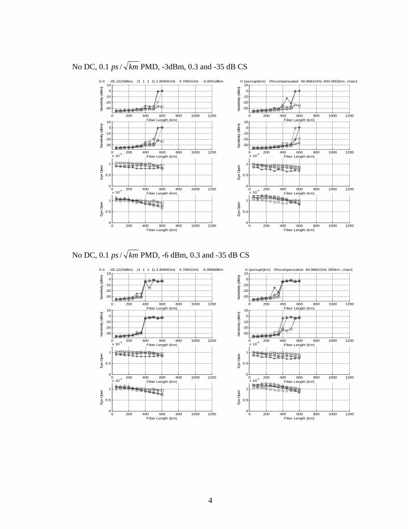
4

No DC, 0.1 kmps / PMD, -3dBm, 0.3 and -35 dB CS

0 200 400 600 800 1000 1200

-30

-20

-10

0

10

Fiber Length (km)

Sen

sitiv

ity (dB

m)

0.3 -35.1223dBsc (1 1 1 1) 2.8094GHz 4.7081GHz -3.0001dBm

0 200 400 600 800 1000 1200

-30

-20

-10

0

10

Fiber Length (km)

Sen

sitiv

ity (dB

m)

0.1ps/sqrt(km) 0%compensated 49.9681GHz 500.0002km, chan1

0 200 400 600 800 1000 1200

-30

-20

-10

0

10

Fiber Length (km)

Sen

sitiv

ity (dB

m)

0 200 400 600 800 1000 1200

-30

-20

-10

0

10

Fiber Length (km)

Sen

sitiv

ity (dB

m)

0 200 400 600 800 1000 12000

0.5

1

x 10-4

Fiber Length (km)

Eye

Ope

n

0 200 400 600 800 1000 12000

0.5

1

x 10-4

Fiber Length (km)

Eye

Ope

n

0 200 400 600 800 1000 12000

0.5

1

x 10-4

Fiber Length (km)

Eye

Ope

n

0 200 400 600 800 1000 12000

0.5

1

x 10-4

Fiber Length (km)

Eye

Ope

n

No DC, 0.1 kmps / PMD, -6 dBm, 0.3 and -35 dB CS

0 200 400 600 800 1000 1200

-30

-20

-10

0

10

Fiber Length (km)

Sen

sitiv

ity (dB

m)

0.3 -35.1223dBsc (1 1 1 1) 2.8094GHz 4.7081GHz -5.9998dBm

0 200 400 600 800 1000 1200

-30

-20

-10

0

10

Fiber Length (km)

Sen

sitiv

ity (dB

m)

0.1ps/sqrt(km) 0%compensated 49.9681GHz 350km, chan1

0 200 400 600 800 1000 1200

-30

-20

-10

0

10

Fiber Length (km)

Sen

sitiv

ity (dB

m)

0 200 400 600 800 1000 1200

-30

-20

-10

0

10

Fiber Length (km)

Sen

sitiv

ity (dB

m)

0 200 400 600 800 1000 12000

0.5

1

x 10-4

Fiber Length (km)

Eye

Ope

n

0 200 400 600 800 1000 12000

0.5

1

x 10-4

Fiber Length (km)

Eye

Ope

n

0 200 400 600 800 1000 12000

0.5

1

x 10-4

Fiber Length (km)

Eye

Ope

n

0 200 400 600 800 1000 12000

0.5

1

x 10-4

Fiber Length (km)

Eye

Ope

n

1

Appendix 5: OC192 resultsDC, 0.1 kmps / PMD, 3dBm, 0.5 and 0 dB CS

0 200 400 600 800 1000 1200-40

-20

0

Fiber Length (km)

Sen

sitiv

ity (dB

m)

0.5 0dBsc (1) 0GHz 7.5175GHz 3dBm

0 200 400 600 800 1000 1200-40

-20

0

Fiber Length (km)

Sen

sitiv

ity (dB

m)

0.1ps/sqrt(km) 100%compensated 49.91GHz 950.0004km, chan3

0 200 400 600 800 1000 1200-40

-20

0

Fiber Length (km)

Sen

sitiv

ity (dB

m)

0 200 400 600 800 1000 1200-40

-20

0

Fiber Length (km)

Sen

sitiv

ity (dB

m)

0 200 400 600 800 1000 12000

2

4

6

x 10-4

Fiber Length (km)

Eye

Ope

n

0 200 400 600 800 1000 12000

2

4

6

x 10-4

Fiber Length (km)

Eye

Ope

n0 200 400 600 800 1000 1200

0

2

4

6

x 10-4

Fiber Length (km)

Eye

Ope

n

0 200 400 600 800 1000 12000

2

4

6

x 10-4

Fiber Length (km)E

ye O

pen

DC, 0.1 kmps / PMD, 0 dBm, 0.5 and 0 dB CS

0 200 400 600 800 1000 1200-40

-20

0

Fiber Length (km)

Sen

sitiv

ity (

dBm

)

0.5 0dBsc (1) 0GHz 7.5175GHz 0dBm

0 200 400 600 800 1000 1200-40

-20

0

Fiber Length (km)

Sen

sitiv

ity (

dBm

)

0.1ps/sqrt(km) 100%compensated 49.91GHz 10000km, chan0

0 200 400 600 800 1000 1200-40

-20

0

Fiber Length (km)

Sen

sitiv

ity (

dBm

)

0 200 400 600 800 1000 1200-40

-20

0

Fiber Length (km)

Sen

sitiv

ity (

dBm

)

0 200 400 600 800 1000 12000

2

4

6

x 10-4

Fiber Length (km)

Eye

Ope

n

0 200 400 600 800 1000 12000

2

4

6

x 10-4

Fiber Length (km)

Eye

Ope

n

0 200 400 600 800 1000 12000

2

4

6

x 10-4

Fiber Length (km)

Eye

Ope

n

0 200 400 600 800 1000 12000

2

4

6

x 10-4

Fiber Length (km)

Eye

Ope

n

2

DC, 0.1 kmps / PMD, -3 dBm, 0.5 and 0 dB CS

0 200 400 600 800 1000 1200-40

-20

0

Fiber Length (km)

Sen

sitiv

ity (dB

m)

0.5 0dBsc (1) 0GHz 7.5175GHz -3.0001dBm

0 200 400 600 800 1000 1200-40

-20

0

Fiber Length (km)

Sen

sitiv

ity (dB

m)

0.1ps/sqrt(km) 100%compensated 49.91GHz 800km, chan1

0 200 400 600 800 1000 1200-40

-20

0

Fiber Length (km)

Sen

sitiv

ity (dB

m)

0 200 400 600 800 1000 1200-40

-20

0

Fiber Length (km)

Sen

sitiv

ity (dB

m)

0 200 400 600 800 1000 12000

2

4

6

x 10-4

Fiber Length (km)

Eye

Ope

n

0 200 400 600 800 1000 12000

2

4

6

x 10-4

Fiber Length (km)

Eye

Ope

n

0 200 400 600 800 1000 12000

2

4

6

x 10-4

Fiber Length (km)

Eye

Ope

n

0 200 400 600 800 1000 12000

2

4

6

x 10-4

Fiber Length (km)

Eye

Ope

n

DC, 0.1 kmps / PMD, -6 dBm, 0.5 and 0 dB CS

0 200 400 600 800 1000 1200-40

-20

0

Fiber Length (km)

Sen

sitiv

ity (dB

m)

0.5 0dBsc (1) 0GHz 7.5175GHz -5.9998dBm

0 200 400 600 800 1000 1200-40

-20

0

Fiber Length (km)

Sen

sitiv

ity (dB

m)

0.1ps/sqrt(km) 100%compensated 49.91GHz 500.0002km, chan1

0 200 400 600 800 1000 1200-40

-20

0

Fiber Length (km)

Sen

sitiv

ity (dB

m)

0 200 400 600 800 1000 1200-40

-20

0

Fiber Length (km)

Sen

sitiv

ity (dB

m)

0 200 400 600 800 1000 12000

2

4

6

x 10-4

Fiber Length (km)

Eye

Ope

n

0 200 400 600 800 1000 12000

2

4

6

x 10-4

Fiber Length (km)

Eye

Ope

n

0 200 400 600 800 1000 12000

2

4

6

x 10-4

Fiber Length (km)

Eye

Ope

n

0 200 400 600 800 1000 12000

2

4

6

x 10-4

Fiber Length (km)

Eye

Ope

n

3

No DC, 0.1 kmps / PMD, 3dBm, 0.5 and 0 dB CS

0 200 400 600 800 1000 1200-40

-20

0

Fiber Length (km)

Sen

sitiv

ity (dB

m)

0.5 0dBsc (1) 0GHz 7.5175GHz 3dBm

0 200 400 600 800 1000 1200-40

-20

0

Fiber Length (km)

Sen

sitiv

ity (dB

m)

0.1ps/sqrt(km) 0%compensated 49.91GHz 100km, chan1

0 200 400 600 800 1000 1200-40

-20

0

Fiber Length (km)

Sen

sitiv

ity (dB

m)

0 200 400 600 800 1000 1200-40

-20

0

Fiber Length (km)

Sen

sitiv

ity (dB

m)

0 200 400 600 800 1000 12000

2

4

6

x 10-4

Fiber Length (km)

Eye

Ope

n

0 200 400 600 800 1000 12000

2

4

6

x 10-4

Fiber Length (km)

Eye

Ope

n

0 200 400 600 800 1000 12000

2

4

6

x 10-4

Fiber Length (km)

Eye

Ope

n

0 200 400 600 800 1000 12000

2

4

6

x 10-4

Fiber Length (km)

Eye

Ope

n

No DC, 0.1 kmps / PMD, 0 dBm, 0.5 and 0 dB CS

0 200 400 600 800 1000 1200-40

-20

0

Fiber Length (km)

Sen

sitiv

ity (

dBm

)

0.5 0dBsc (1) 0GHz 7.5175GHz 0dBm

0 200 400 600 800 1000 1200-40

-20

0

Fiber Length (km)

Sen

sitiv

ity (

dBm

)

0.1ps/sqrt(km) 0%compensated 49.91GHz 100km, chan1

0 200 400 600 800 1000 1200-40

-20

0

Fiber Length (km)

Sen

sitiv

ity (

dBm

)

0 200 400 600 800 1000 1200-40

-20

0

Fiber Length (km)

Sen

sitiv

ity (

dBm

)

0 200 400 600 800 1000 12000

2

4

6

x 10-4

Fiber Length (km)

Eye

Ope

n

0 200 400 600 800 1000 12000

2

4

6

x 10-4

Fiber Length (km)

Eye

Ope

n

0 200 400 600 800 1000 12000

2

4

6

x 10-4

Fiber Length (km)

Eye

Ope

n

0 200 400 600 800 1000 12000

2

4

6

x 10-4

Fiber Length (km)

Eye

Ope

n

4

No DC, 0.1 kmps / PMD, -3dBm, 0.5 and 0 dB CS

0 200 400 600 800 1000 1200-40

-20

0

Fiber Length (km)

Sen

sitiv

ity (dB

m)

0.5 0dBsc (1) 0GHz 7.5175GHz -3.0001dBm

0 200 400 600 800 1000 1200-40

-20

0

Fiber Length (km)

Sen

sitiv

ity (dB

m)

0.1ps/sqrt(km) 0%compensated 49.91GHz 100km, chan1

0 200 400 600 800 1000 1200-40

-20

0

Fiber Length (km)

Sen

sitiv

ity (dB

m)

0 200 400 600 800 1000 1200-40

-20

0

Fiber Length (km)

Sen

sitiv

ity (dB

m)

0 200 400 600 800 1000 12000

2

4

6

x 10-4

Fiber Length (km)

Eye

Ope

n

0 200 400 600 800 1000 12000

2

4

6

x 10-4

Fiber Length (km)

Eye

Ope

n

0 200 400 600 800 1000 12000

2

4

6

x 10-4

Fiber Length (km)

Eye

Ope

n

0 200 400 600 800 1000 12000

2

4

6

x 10-4

Fiber Length (km)

Eye

Ope

n

No DC, 0.1 kmps / PMD, -6 dBm, 0.5 and 0 dB CS

0 200 400 600 800 1000 1200-40

-20

0

Fiber Length (km)

Sen

sitiv

ity (dB

m)

0.5 0dBsc (1) 0GHz 7.5175GHz -5.9998dBm

0 200 400 600 800 1000 1200-40

-20

0

Fiber Length (km)

Sen

sitiv

ity (dB

m)

0.1ps/sqrt(km) 0%compensated 49.91GHz 100km, chan1

0 200 400 600 800 1000 1200-40

-20

0

Fiber Length (km)

Sen

sitiv

ity (dB

m)

0 200 400 600 800 1000 1200-40

-20

0

Fiber Length (km)

Sen

sitiv

ity (dB

m)

0 200 400 600 800 1000 12000

2

4

6

x 10-4

Fiber Length (km)

Eye

Ope

n

0 200 400 600 800 1000 12000

2

4

6

x 10-4

Fiber Length (km)

Eye

Ope

n

0 200 400 600 800 1000 12000

2

4

6

x 10-4

Fiber Length (km)

Eye

Ope

n

0 200 400 600 800 1000 12000

2

4

6

x 10-4

Fiber Length (km)

Eye

Ope

n